enabling technologies for internet of things: …...abstract enabling technologies for internet of...
TRANSCRIPT

Enabling Technologies for Internet of Things:
Licensed and Unlicensed Techniques
Mahmoud Elsaadany
A Thesis
In the Department
of
Electrical and Computer Engineering
Presented in Partial Fulfillment of the Requirements
For the Degree of
Doctor of Philosophy (Electrical and Computer Engineering) at
Concordia University
Montreal, Quebec, Canada
April, 2018
c⃝ Mahmoud Elsaadany, 2018

CONCORDIA UNIVERSITY
SCHOOL OF GRADUATE STUDIES
This is to certify that the thesis prepared
By: Mahmoud Elsaadany
Entitled: Enabling Technologies for Internet of Things:
Licensed and Unlicensed Techniques
and submitted in partial fulfillment of the requirements for the degree of
Doctor of Philosophy (Electrical and Computer Engineering)
complies with the regulations of the University and meets the accepted standards with
respect to originality and quality.
Signed by the final examining committee:
Dr. De Visscher
Chair
Dr. Claude D’Amours
External Examiner
Dr. A. Stancu
External to Program
Dr. M.R. Soleymani
Examiner
Dr. Y.R. Shayan
Examiner
Dr. W. Hamouda
Thesis Supervisor
Approved by:Dr. W.-P. Zhu, Graduate Program Director
May 24, 2018
Dr. A. Asif, Dean, Faculty of Engineering & Computer Science

ABSTRACT
Enabling Technologies for Internet of Things: Licensed and Unlicensed
Techniques
Mahmoud Elsaadany, Ph.D.
Concordia University, 2018
The Internet of Things (IoT) is a novel paradigm which is shaping the evolution of the
future Internet. According to the vision underlying the IoT, the next step in increasing
the ubiquity of the Internet, after connecting people anytime and everywhere, is to connect
inanimate objects. By providing objects with embedded communication capabilities and
a common addressing scheme, a highly distributed and ubiquitous network of seamlessly
connected heterogeneous devices is formed, which can be fully integrated into the current
Internet and mobile networks, thus allowing for the development of new intelligent services
available anytime, anywhere, by anyone and anything. Such a vision is also becoming known
under the name of Machine-to-Machine (M2M), where the absence of human interaction in
the system dynamics is further emphasized.
A massive number of wireless devices will have the ability to connect to the Internat
through the IoT framework. With the accelerating pace of marketing such framework, the
new wireless communications standards are studying/proposing solutions to incorporate the
services needed for the IoT. However, with an estimate of 30 billion connected devices, a lot
of challenges are facing the current wireless technology.
In our research, we address a variety of technology candidates for enabling such a massive
framework. Mainly, we focus on the underlay cognitive radio networks as the unlicensed
candidate for IoT. On the other hand, we look into the current efforts done by the standard-
ization bodies to accommodate the requirements of the IoT into the current cellular networks.
Specifically, we survey the new features and the new user equipment categories added to the
physical layer of the LTE-A.
iii

In particular, we study the performance of a dual-hop cognitive radio network sharing the
spectrum of a primary network in an underlay fashion. In particular, the cognitive network
consists of a source, a destination, and multiple nodes employed as amplify-and-forward
relays. To improve the spectral efficiency, all relays are allowed to instantaneously transmit
to the destination over the same frequency band. We present the optimal power allocation
that maximizes the received signal-to-noise ratio (SNR) at the destination while satisfying
the interference constrains of the primary network. The optimal power allocation is obtained
through an eigen-solution of a channel-dependent matrix, and is shown to transform the
transmission over the non-orthogonal relays into parallel channels. Furthermore, while the
secondary destination is equipped with multiple antennas, we propose an antenna selection
scheme to select the antenna with the highest SNR. To this end, we propose a clustering
scheme to subgroup the available relays and use antenna selection at the receiver to extract
the same diversity order. We show that random clustering causes the system to lose some of
the available degrees of freedom. We provide analytical expression of the outage probability
of the system for the random clustering and the proposed maximum-SNR clustering scheme
with antenna selection. In addition, we adapt our design to increase the energy-efficiency of
the overall network without significant loss in the data rate.
In the second part of this thesis, we will look into the current efforts done by the stan-
dardization bodies to accommodate the requirements of the IoT into the current cellular
networks. Specifically, we present the new features and the new user equipment categories
added to the physical layer of the LTE-A. We study some of the challenges facing the LTE-A
when dealing with Machine Type communications (MTC). Specifically, the MTC Physical
Downlink control channel (MPDCCH) is among the newly introduced features in the LTE-A
that carries the downlink control information (DCI) for MTC devices. Correctly decoding
the MPDCCH, mainly depends on the channel estimation used to compensate for the channel
errors during transmission, and the choice of such technique will affect both the complexity
and the performance of the user equipment. We propose and assess the performance of a
simple channel estimation technique depends in essence on the Least Squares (LS) estimates
of the pilots signal and linear interpolations for low-Doppler channels associated with the
MTC application.
iv

Acknowledgments
First and foremost, all praise and thanks are due to Allah for giving me the strength to keep
trying, and for surrounding me with very supportive personals.
I would like to express my great gratitude to my supervisor Prof. Walaa Hamouda for
being such a great advisor, and for all the support he provided me both technically and
personally. His support and insightful advices were crucial to my academic achievement and
my development as an independent researcher. Honestly, I consider Prof. Hamouda as an
elder brother not only a supervisor or a teacher. Prof. Walaa, thank you for all the technical
and ethical values I have learned from you.
I am also thankful to my friends, Shoukry Shams and Abdelmohsen Ali, for their help
and support.
I am sincerely thankful to Concordia Graduate Student Support Program (GSSP) for
partially funding my PhD’s studies.
Finally, I would like to express my greatest and deepest appreciation to my family, spe-
cially my wife. She has been such a huge support for me and my small family while I was
away. Marwa, thank you for being my co-pilot.
v

To my beloved wife, Marwa Abdelaziz,
To my kids Abdelrahman and Omar,
and to my parents
vi

Contents
List of Figures . . . . . . . . . . . . . . . . . . . . . . . . . . . . . . . . . . . . . . xi
List of Tables . . . . . . . . . . . . . . . . . . . . . . . . . . . . . . . . . . . . . . xvi
List of Symbols . . . . . . . . . . . . . . . . . . . . . . . . . . . . . . . . . . . . . xvii
List of Acronyms . . . . . . . . . . . . . . . . . . . . . . . . . . . . . . . . . . . . xix
1 Chapter 1: Introduction 1
1.1 Machine Type Communications and Internet-of-Things . . . . . . . . . . . . 1
1.2 IoT Applications . . . . . . . . . . . . . . . . . . . . . . . . . . . . . . . . . 2
1.3 Candidate Technologies for IoT . . . . . . . . . . . . . . . . . . . . . . . . . 3
1.3.1 Unlicensed Technologies . . . . . . . . . . . . . . . . . . . . . . . . . 4
1.3.2 Licensed Technologies . . . . . . . . . . . . . . . . . . . . . . . . . . 6
1.4 Unlicensed Access and Cognitive Radios . . . . . . . . . . . . . . . . . . . . 7
1.5 Cognitive Networks . . . . . . . . . . . . . . . . . . . . . . . . . . . . . . . . 8
1.5.1 Underlay Cognitive Networks . . . . . . . . . . . . . . . . . . . . . . 9
1.5.2 Overlay Cognitive Networks . . . . . . . . . . . . . . . . . . . . . . . 9
1.5.3 Interweave Cognitive Networks . . . . . . . . . . . . . . . . . . . . . 9
1.6 Motivation . . . . . . . . . . . . . . . . . . . . . . . . . . . . . . . . . . . . . 10
1.7 Thesis Contributions . . . . . . . . . . . . . . . . . . . . . . . . . . . . . . . 11
1.8 Thesis Organization . . . . . . . . . . . . . . . . . . . . . . . . . . . . . . . . 12
2 Chapter 2: Background and Literature Review 15
2.1 Introduction . . . . . . . . . . . . . . . . . . . . . . . . . . . . . . . . . . . . 15
2.2 Cognitive Radio Systems . . . . . . . . . . . . . . . . . . . . . . . . . . . . . 15
2.2.1 Cognitive Capability . . . . . . . . . . . . . . . . . . . . . . . . . . . 16
2.2.2 Reconfigurability . . . . . . . . . . . . . . . . . . . . . . . . . . . . . 17
vii

2.2.3 Cognitive Networks Architecture . . . . . . . . . . . . . . . . . . . . 17
2.3 Cooperative Communication . . . . . . . . . . . . . . . . . . . . . . . . . . . 18
2.3.1 Amplify-and-Forward . . . . . . . . . . . . . . . . . . . . . . . . . . 18
2.3.2 Decode-and-Forward . . . . . . . . . . . . . . . . . . . . . . . . . . 19
2.3.3 Compress-and-Forward . . . . . . . . . . . . . . . . . . . . . . . . . 19
2.4 Cooperation and Cognitive Radios . . . . . . . . . . . . . . . . . . . . . . . 19
2.4.1 Cooperative Sensing . . . . . . . . . . . . . . . . . . . . . . . . . . . 20
2.4.2 Cognitive Relay Networks . . . . . . . . . . . . . . . . . . . . . . . . 21
2.5 Power Allocation in Underlay Relay Networks . . . . . . . . . . . . . . . . . 23
2.6 LTE Development for MTC and IoT . . . . . . . . . . . . . . . . . . . . . . 24
2.6.1 CAT-0 in Release-12 . . . . . . . . . . . . . . . . . . . . . . . . . . . 26
2.6.2 CAT-M or LTE-MTC in Release-13 . . . . . . . . . . . . . . . . . . . 26
2.6.3 CAT-N or NB-IoT LTE in Release-13 . . . . . . . . . . . . . . . . . . 27
2.7 Physical Layer Features in Legacy LTE Systems . . . . . . . . . . . . . . . . 27
2.7.1 FDD Frame Structure . . . . . . . . . . . . . . . . . . . . . . . . . . 29
2.7.2 Uplink Physical Channels . . . . . . . . . . . . . . . . . . . . . . . . 30
2.7.3 Downlink Physical Channels and Functionalities . . . . . . . . . . . . 33
2.8 Physical Layer Features for LTE-MTC Systems . . . . . . . . . . . . . . . . 40
2.8.1 MTC Features . . . . . . . . . . . . . . . . . . . . . . . . . . . . . . . 41
2.8.2 MTC Physical Random Access Channel (MPRACH) . . . . . . . . . 44
2.8.3 MTC Physical Downlink Control Channel (MPDCCH) . . . . . . . . 45
2.9 Physical Layer Features for NB-IoT Systems . . . . . . . . . . . . . . . . . . 48
2.9.1 Deployment Scenarios and Modes of Operation . . . . . . . . . . . . 48
2.9.2 Downlink Physical Channels . . . . . . . . . . . . . . . . . . . . . . . 49
2.10 Implementation Challenges . . . . . . . . . . . . . . . . . . . . . . . . . . . . 56
2.10.1 Low Power Support . . . . . . . . . . . . . . . . . . . . . . . . . . . . 56
2.10.2 Low Cost Support . . . . . . . . . . . . . . . . . . . . . . . . . . . . 57
2.10.3 System-specific Implementation Aspects . . . . . . . . . . . . . . . . 58
2.11 Conclusion . . . . . . . . . . . . . . . . . . . . . . . . . . . . . . . . . . . . . 60
viii

3 Chapter 3: Power Allocation for Non-Orthogonal Underlay Cognitive
Relay Networks 62
3.1 Introduction . . . . . . . . . . . . . . . . . . . . . . . . . . . . . . . . . . . . 62
3.2 System Model and Assumptions . . . . . . . . . . . . . . . . . . . . . . . . . 63
3.3 Optimal Power Allocation . . . . . . . . . . . . . . . . . . . . . . . . . . . . 65
3.4 Evaluation of The Received SNR . . . . . . . . . . . . . . . . . . . . . . . . 71
3.5 SNR Statistics . . . . . . . . . . . . . . . . . . . . . . . . . . . . . . . . . . . 72
3.5.1 Statistics of γi . . . . . . . . . . . . . . . . . . . . . . . . . . . . . . . 72
3.5.2 Statistics of the received SNR γ∗ . . . . . . . . . . . . . . . . . . . . 74
3.6 Performance Analysis . . . . . . . . . . . . . . . . . . . . . . . . . . . . . . . 78
3.6.1 Outage Probability Analysis . . . . . . . . . . . . . . . . . . . . . . . 78
3.6.2 Bit Error Rate . . . . . . . . . . . . . . . . . . . . . . . . . . . . . . 78
3.7 Numerical Results and Simulation . . . . . . . . . . . . . . . . . . . . . . . . 79
3.8 Power Allocation for Nodes with Individual Power Constraints . . . . . . . . 81
3.8.1 Proposed Power Allocation Algorithm . . . . . . . . . . . . . . . . . 83
3.8.2 Numerical Results . . . . . . . . . . . . . . . . . . . . . . . . . . . . 85
3.9 Energy Efficient Power Allocation . . . . . . . . . . . . . . . . . . . . . . . . 89
3.9.1 Problem Formulation . . . . . . . . . . . . . . . . . . . . . . . . . . . 89
3.9.2 Proposed Solution . . . . . . . . . . . . . . . . . . . . . . . . . . . . 91
3.10 Numerical Results . . . . . . . . . . . . . . . . . . . . . . . . . . . . . . . . . 93
3.11 Summary . . . . . . . . . . . . . . . . . . . . . . . . . . . . . . . . . . . . . 98
4 Chapter 4: Antenna Selection for Dual-hop Cognitive Relay Networks 99
4.1 Introduction . . . . . . . . . . . . . . . . . . . . . . . . . . . . . . . . . . . . 99
4.2 System Model . . . . . . . . . . . . . . . . . . . . . . . . . . . . . . . . . . . 100
4.2.1 Receive Antenna Selection . . . . . . . . . . . . . . . . . . . . . . . . 102
4.2.2 Optimal Beamforming Design . . . . . . . . . . . . . . . . . . . . . . 103
4.3 Clustering . . . . . . . . . . . . . . . . . . . . . . . . . . . . . . . . . . . . . 105
4.3.1 Random Clustering . . . . . . . . . . . . . . . . . . . . . . . . . . . . 105
4.3.2 Max-SNR Clustering . . . . . . . . . . . . . . . . . . . . . . . . . . . 106
ix

4.4 Performance Analysis . . . . . . . . . . . . . . . . . . . . . . . . . . . . . . . 106
4.4.1 Random clustering case: . . . . . . . . . . . . . . . . . . . . . . . . . 106
4.4.2 Max-SNR clustering case: . . . . . . . . . . . . . . . . . . . . . . . . 107
4.5 Simulation Results . . . . . . . . . . . . . . . . . . . . . . . . . . . . . . . . 109
4.5.1 Antenna Selection Only . . . . . . . . . . . . . . . . . . . . . . . . . 109
4.5.2 Effect of Power Allocation Scheme . . . . . . . . . . . . . . . . . . . 110
4.5.3 Relay Clustering and Antenna Selection . . . . . . . . . . . . . . . . 111
4.6 Summary . . . . . . . . . . . . . . . . . . . . . . . . . . . . . . . . . . . . . 115
5 Chapter 5: Channel Estimation for LTE-MTC Systems 116
5.1 Introduction . . . . . . . . . . . . . . . . . . . . . . . . . . . . . . . . . . . . 116
5.2 MTC Physical Downlink Control Channel . . . . . . . . . . . . . . . . . . . 117
5.2.1 MTC Control Channel Assignment . . . . . . . . . . . . . . . . . . . 118
5.3 System and Signal Models . . . . . . . . . . . . . . . . . . . . . . . . . . . . 122
5.4 Channel Estimation For MPDCCH . . . . . . . . . . . . . . . . . . . . . . . 124
5.4.1 Pilot Structure . . . . . . . . . . . . . . . . . . . . . . . . . . . . . . 124
5.4.2 Pilot Signal Estimation . . . . . . . . . . . . . . . . . . . . . . . . . . 125
5.4.3 Proposed Channel Estimation Techniques . . . . . . . . . . . . . . . 128
5.4.4 Repetitions, De-noising and Fast Decoding . . . . . . . . . . . . . . . 129
5.5 Simulation Results . . . . . . . . . . . . . . . . . . . . . . . . . . . . . . . . 131
5.5.1 MPDCCH with Perfect Channel Knowledge . . . . . . . . . . . . . . 131
5.5.2 Proposed Channel Estimation . . . . . . . . . . . . . . . . . . . . . . 132
5.6 Summary . . . . . . . . . . . . . . . . . . . . . . . . . . . . . . . . . . . . . 138
6 Chapter 6: Conclusions and Future Work 139
6.1 Conclusions . . . . . . . . . . . . . . . . . . . . . . . . . . . . . . . . . . . . 139
6.2 Future Work . . . . . . . . . . . . . . . . . . . . . . . . . . . . . . . . . . . . 140
References 142
Appendix: List of Publications 158
x

List of Figures
2.1 Wireless cognitive network with cooperative sensing for the primary activity. 21
2.2 Wireless cognitive network with cooperative transmissions between the sec-
ondary users. . . . . . . . . . . . . . . . . . . . . . . . . . . . . . . . . . . . 23
2.3 Frame structure of legacy LTE systems for FDD with Normal CP type. . . 30
2.4 Frame structure of LTE-MTC systems for FDD with Normal CP type showing
the synchronization signals. The concept of narrowband is highlighted. . . . 43
2.5 Summary for the introduced features for MPDCCH. . . . . . . . . . . . . . . 46
2.6 Radio frame structure for NB-IoT systems. The allocated RB is expanded in
time to show the NPSS/NSSS symbols mapping in addition to the broadcast
channel and one data/control subframe. . . . . . . . . . . . . . . . . . . . . . 50
2.7 Summary for the introduced features for NPDCCH. . . . . . . . . . . . . . . 54
3.1 Underlay Cognitive Relay Network. . . . . . . . . . . . . . . . . . . . . . . . 63
3.2 The average secondary throughput for different values of interference temper-
ature Imax. The system has K = 5 relays. . . . . . . . . . . . . . . . . . . . 69
3.3 The average secondary throughput for different number of secondary relays
K. The interference temperature Imax is set at 10 dB. . . . . . . . . . . . . . 70
3.4 The empirical PDF of γi compared to the proposed exponential approximation
with mean µγ. . . . . . . . . . . . . . . . . . . . . . . . . . . . . . . . . . . . 76
3.5 The empirical PDF of the received SNR γ∗, compared with the proposed
Gamma approximation. . . . . . . . . . . . . . . . . . . . . . . . . . . . . . 77
3.6 The empirical CDF of the received SNR γ∗, compared with the proposed
Gamma approximation. . . . . . . . . . . . . . . . . . . . . . . . . . . . . . 77
xi

3.7 The outage probability Pout of the cognitive network versus γs(dB) for different
values of K. The target SNR γth = 2dB. The interference temperature Imax
is set at 13 dB. . . . . . . . . . . . . . . . . . . . . . . . . . . . . . . . . . . 80
3.8 The outage probability Pout of the cognitive network versus γs(dB) for different
values of γth. The number of relays K = 5. The interference temperature Imax
is set at 13 dB. . . . . . . . . . . . . . . . . . . . . . . . . . . . . . . . . . . 80
3.9 The Average BER Pe of the cognitive network versus γs(dB) for different
values for different values of K. The interference temperature Imax is set at 0
dB. . . . . . . . . . . . . . . . . . . . . . . . . . . . . . . . . . . . . . . . . . 81
3.10 The average secondary throughput for different values of interference temper-
ature Imax. The system has K = 5 relays. . . . . . . . . . . . . . . . . . . . 86
3.11 The average secondary throughput for different number of secondary relays
K. The interference temperature Imax is set to 10 dB. . . . . . . . . . . . . . 87
3.12 The average secondary throughput for different values of the maximum limit
on the secondary source transmission power PSmax for K = 2 and 4. The
interference temperature Imax = 7 dB. . . . . . . . . . . . . . . . . . . . . . 88
3.13 The average secondary throughput for different values of the maximum limit
on the relays’ transmission power Pmax forK = 5 and interference temperature
values of Imax = 3 and 6 dB. . . . . . . . . . . . . . . . . . . . . . . . . . . . 88
3.14 The energy efficiency of the secondary network vs the Secondary source trans-
mission power PS for different network size (K). The interference threshold is
set to 10 dB and the individual relays’ Power Pmax is set to 0 dB. . . . . . . 94
3.15 The outage probability of the secondary system Pout vs the secondary source
transmission power PS for different network size (K).The interference thresh-
old is set to 10 dB and the individual relays’ Power Pmax is set to 0 dB. The
SNR threshold is −3 dB. . . . . . . . . . . . . . . . . . . . . . . . . . . . . . 94
3.16 The energy efficiency of the secondary network vs the interference threshold
Imax for different network size (K). The secondary source transmission power
PS is set to 3 dB and the individual relays’ Power Pmax is set to 3 dB. . . . . 96
xii

3.17 The outage probability of the secondary system Pout vs the interference thresh-
old Imax for different network size (K). The secondary source transmission
power PS is set to 3 dB and the individual relays’ Power Pmax is set to 3 dB.
The SNR threshold is −3 dB. . . . . . . . . . . . . . . . . . . . . . . . . . . 96
3.18 The energy efficiency of the secondary network vs the individual relay power
constraint Pmax for different network size (K). The secondary source trans-
mission power PS is set to 0 dB. The interference threshold Imax is set to 10
dB. . . . . . . . . . . . . . . . . . . . . . . . . . . . . . . . . . . . . . . . . . 97
3.19 The outage probability of the secondary system Pout vs the individual relay
power constraint Pmax for different network size (K). The secondary source
transmission power PS is set to 0 dB. The interference threshold Imax is set to
10 dB, and the SNR threshold is −3 dB. . . . . . . . . . . . . . . . . . . . . 97
4.1 Underlay cognitive relay network with secondary receiver equipped with ND
antennas. . . . . . . . . . . . . . . . . . . . . . . . . . . . . . . . . . . . . . 100
4.2 Outage probability of antenna selection for different values of ND, for number
of relays K = 2 and 3. The interference temperature Imax=7 dB and the
target SNR γth = 3 dB. Solid: Multiple Relays, Dotted: Opportunistic Relay
Selection. . . . . . . . . . . . . . . . . . . . . . . . . . . . . . . . . . . . . . 110
4.3 Outage probability of antenna selection for different power allocation schemes,
with the number of relays K = 3, Imax=7 dB. . . . . . . . . . . . . . . . . . 111
4.4 Outage probability of antenna selection and relay clustering, for different val-
ues of ND, with number of relays K = 6, Imax=7 dB using optimal power
allocation. . . . . . . . . . . . . . . . . . . . . . . . . . . . . . . . . . . . . . 112
4.5 Outage probability of antenna selection and relay clustering vs the number
of relays K while ND is fixed (ND = 2), Imax=7 dB using optimal power
allocation for both random clustering and Max SNR clustering. . . . . . . . 113
4.6 Outage probability of antenna selection and relay clustering vs the number of
antennas ND with K = 20 relays, Imax=3 dB using optimal power allocation. 114
xiii

4.7 Analytical and simulation results of outage probability for K = 12 and differ-
ent ND setups, Imax=5 dB using optimal power allocation for random clustering.114
4.8 Analytical and simulation results of the outage probability for different number
of relays K with ND = 2, Imax=5 dB using optimal power allocation for Max
SNR clustering. . . . . . . . . . . . . . . . . . . . . . . . . . . . . . . . . . . 115
5.1 A single PRB structure for MPDCCH showing locations of DMRS and EREG
start for Normal CP mode. . . . . . . . . . . . . . . . . . . . . . . . . . . . . 118
5.2 Block diagram for the transmitter/receiver model for the control channel sim-
ulation in LTE-MTC system . . . . . . . . . . . . . . . . . . . . . . . . . . . 123
5.3 BLER versus SNR for aggregation level L=2. Different repetition factors,
R ∈ 1, 2, 4, 8, 16, 32, 64, are considered for various channel conditions. . . . 132
5.4 BLER versus SNR for repetition factor R=8. Different aggregation levels,
L ∈ 1, 2, 4, 8, 16, 24, are considered for various channel conditions. . . . . . 133
5.5 BLER versus the repetition factor for a given SNR = -14dB. Different aggrega-
tion levels, L ∈ 1, 2, 4, 8, 16, 24, are considered for various channel conditions. 133
5.6 MSE versus the weight factor α for different SNR = −12dB, −4dB, and 2dB
top to bottom. . . . . . . . . . . . . . . . . . . . . . . . . . . . . . . . . . . 134
5.7 The MSE versus SNR for aggregation level L = 16 of the proposed channel
estimation technique. Different repetitions, R ∈ 16, 64, 128, 256, are con-
sidered for EPA-5 channel. Solid lines are for the channel estimation with
denoising using DFB, and dotted lines are the case of no denoising. . . . . . 135
5.8 BLER versus SNR for aggregation level L = 16. Different repetitions, R ∈
16, 64, 128, 256, are considered for EPA-5 channel using the proposed channel
estimation technique. Solid lines are for the channel estimation with denoising
using DFB, and dotted lines are the case of no denoising. . . . . . . . . . . . 136
xiv

5.9 The index of successful decoding versus SNR for aggregation level L = 16
of the proposed channel estimation technique. Different repetitions, R ∈
16, 64, 128, 256, are considered for EPA-5 channel. Solid lines are for the
channel estimation with denoising using DFB, and dotted lines are the case of
no denoising. . . . . . . . . . . . . . . . . . . . . . . . . . . . . . . . . . . . 137
5.10 Percentage of average successful decoding index to the maximum repetition
factor R. . . . . . . . . . . . . . . . . . . . . . . . . . . . . . . . . . . . . . . 137
xv
List of Tables
1.1 Generic requirements for typical IoT applications. . . . . . . . . . . . . . . . 3
2.1 Summary of the basic requirements for CAT-0, CAT-M, and CAT-N systems 28
2.2 Maximum number of repetitions for different channels. . . . . . . . . . . . . 44
5.1 Candidate Table for CE Mode A in LTE-MTC . . . . . . . . . . . . . . . . . 120
xvi

List of Symbols
S Secondary source
D Secondary destination
K Number of secondary relays
ND Number of receive antennas at the secondary destination
x vector x
X Matrix X
xT Transpose of vector x
X−1 Matrix inverse of matrix X
xi,j Matrix element of row i and column j
EigenX Eigenvalues of the matrix X
TrX The trace of the matrix X
PS Transmission power of S
PRiTransmission power of node Ri
Pmax Maximum transmission power of Secondary nodes
PT Total transmission power
ψRiScaling gain at the node Ri
GRiPhase correction at the node Ri
σ2Ri
Noise variance at the node Ri
CN Complex normal random variable
E[·] The expected value
ga,b The channel coefficient from node a to node b
loga The logarithmic function of base a
R The secondary transmission rate
Imax Interference temperature of the Primary network
|a| The absolute value of a
xvii

max The maximization problem
argmax The maximization problem of the argument function
Γ(a, x) The upper incomplete Gamma function
γ(a, x) The lower incomplete Gamma function
Q(x) Q-function
F (x) Cumulative distribution function
f(x) Probability density function
∈ Within the group
∀ For all
≈ Approximated as
Gm,np,q
⎛⎝ a1, ..., ap
b1, ....., bq
z⎞⎠ The Meijer G-function
Γ(x) The Gamma function
aFb(α, β; γ, z) The Gauss-hypergeometric
Pr(a) Probability of event a
Pe Error probability
Pout Outage probability
γ∗ Optimal SNR of the secondary network
γS Secondary source power relative to noise power
γi The received SNR at the destination D through relay Ri
γth The received SNR threshold at the destination D
γe2e The end-to-end received SNR at the destination D
Cj The jth cluster of secondary relays.
Aj The size of the cluster Cj
h(t, τ) Baseband wireless channel impulse response
Sj(lp, kp) The pilot signal at OFDM symbol lp and subcarrier index kp
hjp Channel estimation at the pilot locations for antenna port j
HMMSE MMSE channel estimation
Bcr The decoded control bits of the received rth repetition
Υ−1 Receiver Processing
xviii

List of Acronyms
3GPP 3rd Generation Partnership Project
ACK Acknowledge
AF Amplify-and-Forward
AP Access Point
AWGN Additive White Gaussian Noise
BER Bit Error Rate
BPSK Binary Phase Shift Keying
BL/CE Bandwidth-reduced Low-complexity and Coverage Extension
CAT-M Category of Machine Type Communications
CAT-N Category of Narrow Band
CF Compress-and-Forward
CDF Cumulative Distribution Function
CP Cyclic Prefix
CR Cognitive Radio
CRN Cognitive Radio Networks
CSCGRV Circularly Symmetric Complex Gaussian Random Variable
CSI Channel State Information
DCI Downlink Control Information
xix

DRX Discontinuous Reception
DSAN Dynamic Spectrum Access Networks
DSP Digital Signal Processor
DF Decode-and-Forward
EPDCCH Enhanced Physical Downlink Control Channel
FCC Federal Communications Commission
FFT Fast Fourier Transform
i.i.d. independent, and identically distributed
ICI Inter Carrier Interference
IFFT Inverse Fast Fourier Transform
IoT Internet of Things
LoRa Long Range
LPWAN Low Power Wide Area Networks
LS Least Squares
LTE Long Term Evolution
LTE-A Long Term Evolution Advanced
M2M Machine to Machine
MAC Medium Access Control
MCL Maximum Coupling Loss
MGF Moments Generating Function
MIMO Multiple Input Multiple Output
xx

MMSE Minimum Mean Squared Error
MSE Mean Squared Error
MPDCCH MTC Physical Downlink Control Channel
MTC Machine Type Communication
NB Narrow band
OFDM Orthogonal Frequency Division Multiplexing
PBCH Physical Broadcast Channel
PDCCH Physical Downlink Control Channel
PDF Probability Density Function
PDSCH Physical Downlink Shared Channel
PSD Power Spectral Density
PSS Primary Synchronization Signal
PRB Physical Resource Block
PU Primary User
PUCCH Physical Uplink Control Channel
PUSCH Physical Uplink Shared Channel
QCQP Quadratically Constrained Quadratic Problem
QoS Quality-of-Service
SDR Software Defined Radio
SNR Signal-to-Noise Ratio
RB Resource Block
xxi

RE Resource Element
RF Radio Frequency
RS Reference Symbol
RSSI Received Signal Strength Indicator
SC-FDMA Single Carrier Frequency Division Multiple Access
SFBC Space-Frequency Block Code
SFO Sampling Frequency Offset
SIMO Single Input Multiple Output
SISO Single Input Single Output
SNR Signal to Noise Ratio
SSS Secondary Synchronization Signal
SU Secondary User
UE User Equipment
xxii

Chapter 1
Introduction
1.1 Machine Type Communications and Internet-of-
Things
The Internet technology has undergone enormous changes since its early stages and it has be-
come an important communication infrastructure targeting anywhere, anytime connectivity.
Historically, human-to-human (H2H) communication, mainly voice communication, has been
the center of importance. Therefore, the current network protocols and infrastructure are
optimized for human-oriented traffic characteristics. Lately, an entirely different paradigm
of communication has emerged with the inclusion of “machines” in the communications
landscape. The exchange of any machine-generated traffic is known as Machine-to-Machine
(M2M) communication [1]. As a result, the speculations about the number of devices ex-
pected to access the Internet in the near future is increasing every day. This is indeed
supported by the Internet-of-Things (IoT) framework being promoted to allow a tremendous
number of “Things” to generate and communicate information among each other without the
need of human interaction [2]. The term “Things” can be used to refer to human services,
machineries (or parts of machines), sensors in smart grids, monitoring devices in e-Health ap-
plications, smart motors/cars or any house hold device in a smart home or a smart city [3] [4].
In terms of M2M communications and IoT features, a new paradigm of networks has to
respect the requirements of machines, such as power and cost [5]. For instance, a set-and-
forget type of application in M2M devices, such as smart meters, require very long battery
life where the device has to operate in an ultra low-power mode [6]. Moreover, the future
network should allow for low complex and low data rate communication technologies which
1

provide low cost devices that encourages the large scale of the IoT. The network architecture,
therefore, needs to be flexible enough to provide these requirements and more.
1.2 IoT Applications
The requirements as to be anticipated vary widely from application to application. However,
there is an effort to categorize applications in a broader framework to provide the best possible
support with an appropriate technical variant of the candidate technologies. A common list
of requirements for IoT use cases can be broadly summarized as follows:
• General requirements of data speeds for both uplink and downlink.
• Relative speed of the IoT device where the application is used
• Tolerance limits on the latency response required for the application.
• Number of reports or readings that are required from the IoT device for the corre-
sponding application.
• Battery requirements for IoT devices that are necessary for a given application.
• Type and extent of security required to preserve the content and communications to
the IoT device.
For example, for applications in the domain of Fleet Management and Logistics, the
typical data rates required are in the range of a few 100s of Kbps, mainly for the uplink.
The IoT application that serves this category needs to ensure that the IoT devices will be
moving at speeds ranging from 10 to 150 Kmph. For these applications, securing real time
and accurate information is of key concern and therefore the tolerance on latency is very low.
The number of reports generated by the IoT devices in this category range from 1 per hour
to 1 per day. Table 1.1 provides a generic requirements for typical IoT applications.
2

Table 1.1: Generic requirements for typical IoT applications.
Application Data Rate Relative
speed
Latency Range
Fleet Management
and Logistics
100s of Kbps High-speed
10-150km/h
Low (Seconds) few km
Automotive Telem-
atics
10s of Mbps Pedestrian:
≤ 5km/h
Low (Seconds) few km
Automation and
Monitoring
50-500kbps Fixed High (Hours) few km
Security and
Surveillance
0.5-8Mbps Fixed Milliseconds few km
Health Monitoring 50-500kbps Pedestrian:
≤5km/h
Low (Seconds) 10s of me-
ters
Wearable (e.g.
sports and data
sharing)
10s of Mbps Pedestrian:
≤5km/h
Low (Seconds) 10s of me-
ters
1.3 Candidate Technologies for IoT
A considerable amount of research has been directed towards available network technologies
such as ZigBee (IEEE 802.15.4), Bluetooth (IEEE 802.15.1), or WiFi (IEEE 802.11b) by
interconnecting devices in a form of large heterogeneous network [7] [8]. Furthermore, solu-
tions for the heterogeneous network architecture (connections, routing, congestion control,
energy-efficient transmission, etc.) have been presented to suit the new requirements of M2M
communications. However, it is still not clear whether these sophisticated solutions can be
applied to M2M communications due to constraints on the hardware complexity, coverage,
and coordination. Indeed, while WiFi, Bluetooth and ZigBee are widely used nowadays
for -more or less- similar applications as M2M communication, the coverage range of these
technologies is very short [9] [10] making them only candidates for some of the applications.
3

Also, operation on unlicensed spectrum forces such technologies to adopt spectrum sensing
techniques (listen-before-talk) or controlled interference (Underlay networks) which affects
the transmission duty cycle.
On the other hand, Low Power Wide Area (LPWA) networks present a good candidate to
support the aforementioned diverse requirements of the IoT framework [11] [12] [13]. A variety
of LPWA technology candidates can overcome the short range constraint of the LAN and still
satisfy the power and latency constraints using either proprietor or cellular technologies (using
licensed or unlicensed spectrum). It seems more efficient to take advantage of the currently
well developed and mature radio access networks. With the large coverage and flexible data
rates offered by cellular systems, research efforts from industry have recently been focused
on optimizing the existing cellular networks considering M2M specifications [14]. Among
the possible solutions, the famous proprietary technologies: Sigfox [15] and LoRa [16], along
with the new developments of the current cellular technologies such as the new categories of
LTE-A user equipments are considered.
Due to the radical change in the number of users, the network has to carefully utilize the
available resources in order to maintain reasonable quality-of-service (QoS). Generally, one
of the most important resources in wireless communications is the frequency spectrum. To
support larger number of connected devices in the future IoT, it is likely to add more degrees
of freedom represented in more operating frequency bands. However, the frequency spectrum
is currently scarce and requiring additional frequency resources makes the problem of sup-
porting this massive number of devices even harder to solve. In fact, this issue is extremely
important especially for the cellular architecture since the spectrum scarcity problem directly
influences the reliability and the QoS offered by the network.
1.3.1 Unlicensed Technologies
1.3.1.1 Sigfox
Sigfox is a French company works with network operators to offer an end-to-end LPWA
connectivity solution based on its patented technologies. Sigfox Network Operators deploy
the proprietary base stations equipped with cognitive software defined radios to operate as a
4

secondary system (unlicensed), and connect them to the back-end servers using an IP-based
network. The connectivity to the base station is simplified and uses only Binary Phase Shift
Keying (BPSK) modulation in an ultra narrow bandwidth (100Hz) in the 868 MHz or 915
MHz ISM band. This way, Sigfox utilizes bandwidth efficiently and promises ultra-low power
consumption, and inexpensive radio frequency (RF) chain designs. However, Sigfox offers
a throughput of only 100bps rendering it a candidate for low traffic applications. Further,
a Sigfox downlink communication can only precede uplink communication after which the
end device should wait to listen for a response from the base station. The number and size
of messages over the uplink are limited to 140 12-byte messages per day to conform to the
regional regulations on use of license-free spectrum.
1.3.1.2 LoRa/LORAWAN
A special interest group constituted from several commercial and industrial partners known
as LoRaTM Alliance proposed LoRaWAN, as an open standard defining the network archi-
tecture and layers above the LoRa physical layer. LoRa (short for Long Range), originally
developed and commercialized by Semtech Corporation [17], is a physical layer technology
that modulates the signals in the industrial, scientific and medical (ISM) radio band. Using
chirp spread spectrum (CSS) technique, a narrow band input signal spread over a wider
channel bandwidth. The resulting signal has noise like properties, making it harder to detect
or jam and hence, at the receiver, the signal enjoys an increased resilience to interference
and noise. LoRa supports multiple spreading factors (between 7-12) to decide the tradeoff
between range and data rate. Higher spreading factors deliver long range at an expense of
lower data rates. Also the combination of Forward Error Correction (FEC) with the spread
spectrum technique to increases the receiver sensitivity. The data rate ranges from 300bps
to 37.5kbps depending on the spreading factor and channel bandwidth. Further, multiple
transmissions using different spreading factors can be received simultaneously by a LoRa base
station. The messages transmitted from end devices are received by multiple base stations,
giving rise to “star-of-stars” topology, and hence improves the probability of successfully
received messages. However, this increases the overhead of the network side as the resulting
duplicate receptions are filtered out in the back-end. Some studies reported the performance
5

of LoRa for outdoor applications [18] [19] [20] and [21] focused on indoor applications.
1.3.1.3 INGENU RPMA
Unlike LoRa and Sigfox, INGENU (also known as On-RampWireless) is a proprietary LPWA
technology that operates in 2.4 GHz ISM band and takes advantage of more relaxed regu-
lations on the unlicensed spectrum use across different regions [22]. INGENU leads efforts
to standardize the physical layer specifications under IEEE 802.15.4k standard [23]. IN-
GENU uses a patented physical access scheme named as Random Phase Multiple Access
(RPMA) [24] Direct Sequence Spread Spectrum, which it employs for uplink communication
only. Using Code Division Multiple Access (CDMA), RPMA enables multiple transmitters
to share a single time slot. However, RPMA increases the duration of time slot of tradi-
tional CDMA and then distributes the channel access within this slot by adding a random
offset delay for each transmitter. By asynchronous access grants, RPMA reduces overlapping
between transmitted signals and thus increases signal to interference ratio for each individ-
ual link [25]. INGENU provides bidirectional communication, although with a slight link
asymmetry. For downlink communication, base stations spread the signals for individual end
devices and then broadcast them using CDMA. Further, the end devices can adjust their
transmit power for reaching closest base station and limiting interference to nearby devices.
1.3.2 Licensed Technologies
Among licensed solutions to enable wireless infrastructure of M2M communications, scenarios
defined by the 3rd Generation Partnership Project (3GPP) standardization body emerge as
the most promising solutions [26]. Due to the M2M communication challenges and the wide
range of supported device specifications, developing the features for M2M communication,
also refers to machine-type-communication (MTC) in the context of Long Term Evolution
(LTE), started as early as release 10 (R10) for the advanced LTE standard [27]. From the
history of M2M communication (in the LTE convention) development, the first generation of a
complete feature MTC device has emerged in R12. In this release, R12, the 3GPP committee
has defined a new profile referred to as category 0 or CAT-0 for low-cost MTC operation [28].
Also a full coverage improvement is guaranteed for all LTE duplex modes. Indeed, the effort
6

continued to future releases including release 13 (R13) that was released late in 2016. In
this front, two special categories, namely CAT-M for MTC and CAT-N for Narrowband-IoT
(NB-IoT), have been incorporated by the 3GPP to LTE specifications to support complete
M2M and IoT features, respectively. The new categories satisfy the general requirements of
MTC and can support the wide range of IoT applications. For example, the capabilities of
the new categories can support applications in the domain of fleet management and logistics,
which require secured, wide range, real time and accurate information with typical data rate
of hundreds of Kbps at speeds ranging from 10 to 150 Km/h. On the other hand, they can
also support applications with very low moving speeds (or stationary) and moderate data
rates with hours of latency, such as, automation and monitoring applications.
1.4 Unlicensed Access and Cognitive Radios
Fixed spectrum allocation is currently used for wireless network, in which a long term as-
signment of the spectrum is made to the license holders in large geographical regions. This
assignment is regulated by governmental agencies. The federal communications commis-
sion (FCC) proved recently, by measurements, that the spectrum is not optimally utilized
[29]. For instance, cellular networks are overloaded while TV spectrum is under-utilized.
Therefore, the apparent scarcity of spectrum is in fact due to inefficient utilization rather
than a shortage of this precious resource. This situation increased the interest in developing
more flexible spectrum usage models rather than the exiting ones. In particular, new ideas
emerged to allow non-licensed users (referred to as secondary users) to be able to utilize
the spectrum allocated to the licence owners (referred to as primary users), as long as the
primary communication is not disturbed.
The term “Cognitive radio” (CR), coined by J. Mitola [30], refers to the technology that
improves the utilization of the spectrum by sharing the resources in an intelligent way. He
proposed a new spectrum usage policy, namely “Spectrum Pooling”, to increase the spectrum
efficiency. The idea of spectrum pooling suggests the license owners to create a pool of their
spectra to bring their idle resources to market. A description of the main properties of CR,
and the ways it may enhance the spectrum utilization are found in the landmark paper of
7

Haykin [31]:
“A cognitive radio is an intelligent wireless communication system that is aware of its sur-
rounding environment, and uses the methodology of understanding-by-building to learn from
the environment and adapt its internal states to statistical variations in the incoming radio
frequency stimuli by making corresponding real time changes in certain operating param-
eters (e.g., transmit power, carrier frequency, and modulation strategy) with two primary
objectives:
• Highly reliable communications whenever and wherever needed.
• Efficient utilization of the radio spectrum.”
Cognitive radios support is a promising solution for supporting massive MTC devices. It can
be argued that cognitive radio concept is a possible solution from the cost and performance
perspectives. However, there are more practical challenges that need efforts from researchers
in order to have a reliable and a mature solution. Future standards are encouraged to provide
both options (i.e. the cognition concept and the heterogeneous/traditional network model).
1.5 Cognitive Networks
While the fixed spectrum allocation cannot hold for the increased number of services and
devices associated with the IoT framework, it was necessary to find a new communication
paradigm to exploit the existing wireless spectrum. Dynamic spectrum access is proposed to
solve the current spectrum crisis. Dynamic Spectrum Access Networks (DSANs)- also known
as cognitive radio networks- can offer spectrum usage to mobile users via heterogeneous
wireless architectures and dynamic spectrum access techniques. The success in applying the
cognitive radio concept is conditioned to find a way to merge the secondary signals with the
primary ones such that the primary users are unaware of the presence of the secondary users.
This merging may take one of these forms: overlay, underlay, or interweave [32]. We discuss
briefly the properties of each approach.
8

1.5.1 Underlay Cognitive Networks
The underlay approach allows concurrent primary and secondary users transmissions by
enforcing the secondary network power level to be below a certain level. This level ensures
secondary network interference to be below the acceptable noise floor of the primary network.
As a result, the underlay systems need to use more bandwidth to provide useful signal to noise
ratio (SNR). Spread spectrum techniques and Ultra-Wide Band (UWB) communications are
proposed to implement this approach [33].
1.5.2 Overlay Cognitive Networks
The overlay approach also allows concurrent primary and secondary transmissions but in a
different way. The most common method of overlay systems allows the secondary users to
assist the primary transmissions. This assistance may take the from of relaying while using
combination of coding schemes such as the Han-Kobayashi coding scheme for the general
interference channel and Costas dirty paper coding as in [34].
1.5.3 Interweave Cognitive Networks
The licensed spectrum bands might be unused for a specific time or at certain location. These
bands are conceptually referred as spectrum holes or white spaces. These holes can be used
for communication by secondary users based on the ability of these users to identify these
holes. Consequently, the utilization of the spectrum is improved by opportunistic frequency
reuse over the spectrum holes. Therefore, an opportunistic cognitive radio is an intelligent
wireless communication system that periodically monitors the radio spectrum to detect occu-
pancy in the different parts of the spectrum, and then opportunistically communicates over
spectrum holes with minimal interference to the primary users. This type of opportunistic
communications is the key idea behind the interweave approach.
9

1.6 Motivation
The key objectives of this thesis are to:
1. Study the challenges for the next generation MTC networks and provide an efficient
solution based on cognitive radio concept for the massive interconnected devices in a
scarce spectrum;
2. Address the practical implementation challenges for the LTE-A cellular support for
MTC;
3. Develop analytical and simulation frameworks for the developed techniques.
The proposed work in this thesis is important in various ways. It certainly addresses a
timely topic (cognitive radio systems in conjunction with cellular MTC and IoT), which is
expected to play a major role in many of the future wireless communication systems. In fact,
this technology is expected to revolutionize how wireless communication networks will be
implemented or deployed in the future, with a focus on addressing the problems of spectrum
under-utilization and supporting numerous number of interconnected MTC devices.
From the merge between the underlay cognitive radios and cooperative communications
an interesting scenario rises, namely “The Underlay Cognitive Relay Networks”. Such type
of networks does not require the overhead of sensing the primary users existence and still
offers a huge increase in the spectrum usage efficiency. However, the main challenge of this
type of networks is how to choose the transmission power level of each and every node in
the network, such that the generated interference due to its existence is not violating the
primary users constraints. Hence, the problem of power allocation of different cognitive
nodes in the relaying network is receiving an increased attention. A lot of effort has been put
into the modeling and the formulation of the power allocation problem over the last decade.
However, due to its complexity, not all of the parameters are included. For example, the focus
of most of the existing work in literature is on single relay networks, although multiple relay
networks offer better performance over single-relay networks for the same amount of feedback.
However, when the multiple relay network problem is addressed, most of the studies focus on
10

subgroup selection and on-off (binary) power allocation. Also, the performance of such type
of networks becomes mathematically intractable, due to the lack of closed form expression
for the statistics of the important parameters in the system, such as the received SNR.
On the other hand, MTC devices are expected to work in environments characterized
by low coverage, ultra low power consumption, and reduced complexity. This will impose a
significant number of implementation challenges on cellular (licensed) networks to support
such requirements. Fore example, the 3GPP standard for LTE-A recently included new
categories of user equipment to support MTC. The new categories can provide low cost, low
power, and extended coverage modes, but at the expense of changing some features in the
physical layer. The introduction of these changes will affect the performance of the currently
used algorithms, such as cell search and channel estimation techniques. New solutions have
to be investigated to proved optimized solutions for the new systems.
1.7 Thesis Contributions
Given the motivating points in the last section, the contributions of this thesis can be sum-
marized as follows.
• A study of the optimal power allocation of an underlay cognitive relay network in order
to maximize the received SNR is provided. The system under consideration employs
multiple amplify-and-forward relays that use the same frequency band simultaneously.
Given an interference threshold on the primary network, we formulate a quadratically
constrained quadratic optimization problem (QCQP). Using this novel formulation, we
obtain the optimal power allocation at the different cognitive nodes. Our results show
that the obtained power allocation transforms the non-orthogonal relaying channel into
parallel channels. We also study the energy efficiency of the proposed power allocation,
and provide new algorithms to enhance this efficiency.
• We assess the performance of the cognitive system while employing multiple antennas at
the destination. We propose approximating the individual SNRs as exponential random
variables using moment matching method. Hence, the received SNR is approximated as
11

a Gamma random variable. For this approximation, we provide closed-form expressions
for the performance of the cognitive system in terms of the outage probability and bit
error rate.
• Finally, we will look into the current efforts done by the standardization bodies to
accommodate the requirements of the IoT into the current cellular networks. Specifi-
cally, we present the new features and the new user equipment categories added to the
physical layer of the LTE-A. We study some of the challenges facing the LTE-A when
dealing with Machine Type communications (MTC). Specifically, the MTC Physical
Downlink control channel (MPDCCH) is among the newly introduced features in the
LTE-A that carries the downlink control information (DCI) for MTC devices. Correctly
decoding the MPDCCH, mainly depends on the channel estimation used to compensate
for the channel errors during transmission, and the choice of such technique will affect
both the complexity and the performance of the user equipment. Therefore, here, we
propose and assess the performance of a simple channel estimation technique based
on the Least Squares (LS) estimates of the pilots signal and linear interpolations for
low-Doppler channels associated with the MTC application.
1.8 Thesis Organization
The rest of the thesis is organized as follows:
In Chapter 2, we present a background on the cognitive radio systems, a literature review
about different types of cooperation among cognitive nodes, and the existing power alloca-
tion schemes in underlay cognitive relay networks. Then, we introduce the basic concepts
of physical LTE systems and its relevant transmission technique, namely the Orthogonal
Frequency Division Multiplexing (OFDM). The essential information about the MTC and
NB-IoT categories are also covered. In the last part of this chapter, we provide the related
works to this research in the literature. We also present the major challenges of future M2M
cellular networks such as spectrum scarcity problem, support for low-power, low-cost, and
numerous number of devices. As being an integral part of the future IoT, the true vision of
M2M communications cannot be reached with conventional solutions that are typically cost
12

inefficient. To this extent, we present a complete fundamental understanding and engineering
knowledge of cognitive radios, and power and cost challenges in the context of future M2M
cellular networks.
In Chapter 3, we address the power allocation for non-orthogonal cognitive relay networks.
We first introduce the system model and assumptions. Then, the formulation of the power
allocation problem and the proposed solution are provided, along with the analysis of the
statistics of the received SNR and the system performance. We also present assessment of
the performance of the system through simulation and analytical expressions. Finally, we
address an energy-efficient design for the proposed power allocation.
In Chapter 4, we study the underlay cognitive network while the secondary destination
has multiple antennas. To reduce the overall system complexity, we propose using antenna
selection and relay clustering. We introduce a novel criterion for antenna selection to max-
imize the received SNR at the secondary destination. We present the outage performance
of the system while utilizing multiple non-orthogonal relays (forming a distributed antenna
system) and antenna selection at the destination. While the optimal beamforming using all
the available relays enhance the performance by allowing more degrees of freedom to the
system designer, it suffers from increased complexity. As a solution, we propose a clustering
scheme to subgroup the available relays and use antenna selection at the receiver to extract
the same diversity order. We show that random clustering results in lose of some of the avail-
able degrees of freedom. Hence, we propose a new technique for clustering, namely Max-SNR
clustering, to jointly associate subset of relays to one of the receive antennas and select the
antenna that provides the maximum SNR. We provide a closed-form analytical expression of
the outage probability of the system for the random clustering and the proposed Max-SNR
clustering schemes with antenna selection.
In Chapter 5, we mainly address challenges for the practical implementation side of LTE-
MTC systems. In particular, we study the concepts of MPDCCH compared to the legacy
EPDCCH. This includes the resource allocation, the new involved downlink control informa-
tion formatting, the concept of frequency hopping, the repetition, and others. We propose
a channel estimation algorithm for the newly introduced MPDCCH in the specifications of
the LTE-A CAT-M. The proposed technique aims at reducing the complexity of the channel
13

estimation of the MPDCCH as minimum as possible. In order to achieve this goal, we pro-
pose using the simple Least-Squares (LS) estimation to estimate the pilots signals, followed
by two stage first-order polynomial interpolation (linear) to obtain the channel estimates at
every point in the time-frequency grid. We also propose using the repeated transmissions (in
case of coverage enhancement mode) to enhance the performance of the proposed technique.
In Chapter 6, we present a brief summery of our investigation and some important con-
clusions. We also suggest some potential topics for future research.
14

Chapter 2
Background and Literature Review
2.1 Introduction
In this chapter, a background for the main topics of this thesis is given. First, we present an
overview of cognitive radio systems as a candidate enabling IoT through unlicensed access.
We present the cognitive radio properties, the cognitive network setup and architecture, and
a literature survey on cooperative cognitive radio networks is given. We also highlight the
concept of cognitive relaying and summarize recent works relate to the problems studied
in this thesis. Next, we give a background about one of the major candidates to support
cellular connections for MTC and IoT applications, namely LTE-A. We start by introducing
the basic concepts of legacy LTE systems and their physical layer transmission techniques for
different channels. Then, the essential information related to the new MTC and NB-IoT user
categories are covered. In the last part of this chapter, we discuss some of the implementation
challenges that will be studied in this thesis.
2.2 Cognitive Radio Systems
A huge demand for bandwidth is expected to grow in the future triggered by the anticipated
increased number of wireless devices through the IoT framework [32]. Spectrum licensing
has been the traditional approach to ensure the coexistence of diverse wireless systems. An
alternative technology, enabling new coexistence approaches, is receiving increased attention
in recent wireless communication research literature, namely “Cognitive Radios”. The at-
tractive feature in cognitive radios is its promise to increase the spectrum utilization. This
15

promise is driven mainly by the ability of the cognitive radios to coexist with traditional spec-
trum owners (primary or licensed users) and share the spectrum band in an opportunistic
fashion. This ability is conditioned to not altering the operation of licensed users or nega-
tively affecting their performance. The idea behind the cognitive radio concept was initiated
by the ability to build a “Software Defined Radio” (SDR). In SDRs, a radio architecture uses
powerful computational resources available in Digital Signal Processors (DSPs) and General
Purpose Processors (GPPs) to implement the modulation and demodulation and all of the
signaling protocols of a radio as a software function [35].
The term Cognitive radio was coined by J. Mitola [30]. The main focus was on the radio
knowledge representation language (RKRL) and how the cognitive radio can enhance the
flexibility of personal wireless services. One description of the main properties of CR, and
the ways it may enhance the spectrum utilization is given in [36]:
“A Cognitive Radio is a radio that can change its transmitter parameters based on inter-
action with the environment in which it operates”.
Cognition can be associated with machine learning [37], which uses any algorithm that
improves the performance through experience gained over a period of time without complete
information about the operation environment of the radio. Adaptive decision making algo-
rithms can be used to give cognitive networks a wide scope of possible mechanisms to use
for learning. Learning serves to complement the objective optimization part of the cognitive
process by retaining the effectiveness of past decisions under a given set of conditions. Out
of this description, we can obtain the two main properties of the cognitive radio as follows.
2.2.1 Cognitive Capability
Cognitive capability refers to the ability of the radio technology to collect information from its
radio environment in a real time fashion. This capability may not be the simple monitoring
of the power spectral density in the band of interest, but it might require more sophisticated
techniques in order to avoid interference to other users as well as capturing the variations
in the radio environment. Through this capability, the spectrum bands that are not used
at a specific time or location can be identified. This concept is referred as spectrum hole
or white space. Following spectrum holes identification, the node can select best spectrum
16

and appropriate operating parameters for the required service. The cognitive capability
is divided into three main processes referred as the cognition cycle. These processes are
spectrum sensing, spectrum analysis and spectrum decision [38]:
• Spectrum sensing: cognitive radio monitors the available spectrum bands and detect
the spectrum holes.
• Spectrum analysis: The characteristics of the spectrum holes that are detected through
spectrum sensing are estimated.
• Spectrum decision: Depending on the analysis, a cognitive radio determines the data
rate, the transmission mode, and the bandwidth of the transmission.
2.2.2 Reconfigurability
Real time interaction with the environment is required as the spectrum holes locations change
temporally and spatially. Reconfigurability is the ability of adjusting transmission parameters
on real time basis without any modifications in the hardware components. This capability
enables the cognitive radio to adapt easily to the dynamic radio environment. The operating
frequency, modulation, transmission power and the communication technology may be incor-
porated into the reconfigurable parameters that cognitive radio can adapt to accommodate
for the environmental changes.
2.2.3 Cognitive Networks Architecture
Developing the cognitive radio networks communication protocols requires a clear identifica-
tion of network elements. The network architecture of the cognitive radio networks consists
of two main components: the primary network and the secondary network. The primary
network is licensed to use a certain spectrum band while the secondary network is the un-
licensed network attempting to share the same spectrum with the primary network. The
primary network users should not be affected by the presence of the secondary network
users. On the other hand, the secondary network users should make use of cognitive radio
abilities to perform all functions necessary to coexist with the primary network. They are
17

required to protect the primary network from interference that could happen due to the
existence of the secondary network.
2.3 Cooperative Communication
Multiple-input multiple-output (MIMO) systems are able to significantly improve the per-
formance of wireless systems (e.g., increase data rate, reduce interference, and improve link
reliability) by means of diversity. However, due to cost, size or hardware limitations, multiple
antennas might not be applicable for some network nodes. For such scenarios, user coopera-
tion can create a virtual MIMO system and thus enabling a single-antenna user to gain the
benefits of MIMO systems. Transmissions via cooperation can be typically modeled as a tra-
ditional relay channel. A literature survey on relay channels can be traced back to the seminar
paper by Cover and El Gamal in [39], in which the capacity region was determined for the
Gaussian single relay network case. Cooperative communications can be accomplished via a
wireless network consisting of geographically separated nodes (relays) cooperating in order to
improve system performance. The interest in relay networks has recently increased from sev-
eral different perspectives. Modeling of link abstractions at higher layers in a communication
system, coding, synchronization, and signal processing designs within a physical layer are
the common research areas in this context. Different cooperative communications protocols
have been proposed which can be found in [40]- [41], and in the references therein. In the
following, we discuss briefly the most common strategies for cooperative communication.
2.3.1 Amplify-and-Forward
In amplify-and-forward (AF), the relay simply amplifies the received signal and forward the
scaled signals to the destination [41]. This method is often used when the relays have limited
resources, e.g. processing time or power. The idea behind AF relaying is simple. During
the first interval, the transmitter sends it signal to the relays. Then each relay multiplies its
received signal by a coefficient and during the second interval forwards it to the destination.
In this process, noise at each relay is also amplified.
18

2.3.2 Decode-and-Forward
In decode-and-forward (DF), each relay decodes the entire received message, re-encodes it
and sends the resulting sequence to the destination [42]. In this strategy, each relay should
know the codebook used by the source in order to be able to decode and re-encode the
received message. The output of each relay acts like an exact copy of the source message.
The performance of DF outperforms AF (in case of error-free decoding), at the expense of
increased complexity in the signaling communications to establish the knowledge about the
used codes.
2.3.3 Compress-and-Forward
In compress-and-forward (CF), the relay transmits a quantized and compressed version of
the received signal to the destination. The destination, then, decodes the desired signal by
combining the received signal from the relay and the directly received signal from the source.
Although the DF strategy is optimal for degraded relay channels [39], the CF strategy is
more powerful when the channel between the relay and destination nodes is good enough
[43]. For Gaussian relay channels, an achievable rate for the CF strategy is explicitly shown
in [44].
2.4 Cooperation and Cognitive Radios
As the primary users have privileged access to the common channel, there are a lot of technical
challenges facing the cognitive radios such as:
Spectrum sensing: In case of interweave cognitive radios, secondary users need to monitor
the available spectrum or a portion of it in order to be able to detect the white spaces.
A typical way to address the problem is to detect the primary transmissions by using a
signal detector. The trade-off between probability of false alarm and missed detection
is reflected in either: missing transmission opportunities or in increasing interference
level to the primary [45]- [46]. The main issue is to enable quick and effective detection
at all the secondary nodes that can potentially interfere with the primary transmission.
19

Also detecting or locating the primary receivers is a major problem [47]. The impact
of practical limitations in spectrum sensing on the performance of cognitive radio from
a system perspective have been investigated in [48].
Resources allocation: In case of underlay cognitive radios, secondary users need to exploit
the transmission opportunity while satisfying two conflicting objectives:
• Making their activity transparent to the primary users (according to a defined
criterion for transparency, such as keeping the interference level below a given
threshold).
• Maximize their own performance in terms of the desired QoS (e.g., rate, delay,
etc.).
Secondary users might be competing for the resource, or cooperating in order to improve
efficiency and fairness of resource sharing. A solution for both problems illustrated
above can greatly benefit from cooperation among different secondary terminals.
In the following, we present some of the possible scenarios where cognitive radios make
use of cooperation to enhance their performance.
2.4.1 Cooperative Sensing
One of the major problems in the primary user activity detection is the low SNR of the
received signal at the cognitive user. This low SNR leads to longer sensing times especially
in energy detectors. Even with infinite sensing time, the detection may be impossible with the
signal SNR is below a certain limit [49]. Enhancing the performance of primary detection
requires a solution that can mitigate poor channel conditions, which is achieved through
“Cooperation” [50]- [51]. The basic idea is to employ distributed detection at the secondary
nodes with each node measuring the local received signal. Then local signals are exchanged
to a central point and finally a global decision on the primary activity is achieved, as shown
in figure 2.1. This approach is clearly robust to possible unbalance of the channel qualities
of different secondary users and can achieve better detection performance. In [52], Ghasemi
et al proposed the use of cooperative transmission to enhance the sensing process. The main
20

Primary Link
Secondary Network
Figure 2.1: Wireless cognitive network with cooperative sensing for the primary activity.
idea is to let the secondary relay node amplify-and-forward the received signal as it contains
not only the transmission from the secondary source, but also the signal from the primary.
This relayed signal allows the secondary destination to improve the detection of the primary
user if the relay is placed approximately halfway between the primary transmitter and the
secondary destination.
2.4.2 Cognitive Relay Networks
Cooperative transmission in its basic forms refers to the information theoretic model of the
“Relay Channel”, where one node (the relay) forwards the transmission of another node
(the source) towards the intended destination. Performance advantages achievable from
collaboration arise from:
• Power gains, that can be harnessed if the relay happens to be in a convenient location,
typically halfway between source and destination.
• Diversity gains, that leverage the double path followed by the signal (direct source-
destination and relay transmissions) [50]. In the context of cognitive radio, cooperative
21

transmission between the nodes gives rise to the cognitive relays networks.
In cognitive relay networks, single or multiple secondary users forward the transmission of
another secondary terminal to the destination (see figure 2.2). All the secondary nodes should
keep the interference to the primary network within allowed limits.
In [53], the outage performance of a cognitive wireless relay network is investigated. The
model used consists of a source node, a destination node, and a group of network clusters
each consisting of a number of cognitive (unlicensed) relay nodes and a primary (licensed)
node. Cognitive nodes relay information from the source depending on their geographical
proximity and their ability to acquire the spectrum hole successfully. Also, an investigation
of the high SNR approximation of the outage probability of the dual-hop system to obtain
the diversity order is performed. A full diversity gain is achieved only if each relay node
successfully identifies the spectrum hole unoccupied by the corresponding primary node in
the cluster. However, the imperfect spectrum acquisition is proved to have a negatively
significant effect on the diversity order.
Improving the outage performance of the network can be achieved by incorporating a
specific intra-cluster cooperation scheme where neighboring cognitive relay nodes in a cluster
collaborate with a desired cognitive relay node. The combination of this intra-cluster cooper-
ation improves the outage performance significantly, and the full diversity can be achieved if
the proper number of neighboring relay nodes participate in the intra-cluster cooperation. In
the invited paper [54], Leila et al investigated the performance gains of cognitive radio relay
networks under QoS limitations at the secondary users, and spectrum sharing restrictions
imposed by the primary users. In their model, secondary users are allowed to gain access to
the licensed spectrum band as long as a limit on the primary outage probability is satisfied.
An interesting approach is to allow relay selection (from K nodes) by the secondary transmit-
ter to amplify and forward its signal to the destination. Considering that the transmission
of the secondary user has to satisfy a statistical delay QoS constraint, the effective capacity
of the relaying link degrades as the QoS constraint gets more tight. However, increasing the
number of relaying nodes (K) results in an increase of effective capacity. The slope of the
effective capacity gain decreases as K increases, indicating that over-dense relay networks do
not gain effective capacity as low density ones.
22

Primary Link
Secondary Network
Figure 2.2: Wireless cognitive network with cooperative transmissions between the secondary
users.
2.5 Power Allocation in Underlay Relay Networks
With the advantage offered by cooperative communication, the bottleneck that limits the
throughput and coverage of underlay cognitive users, is the imposed limitations on their
transmitted powers [55]. Therefore, several studies have been conducted to analyze the per-
formance of cooperation among underlay cognitive nodes considering different limitations on
the interference and the used transmission powers. For example, the effect of the interference
constraint on the diversity gain in DF relaying networks is studied in [56].
In [57], the achievable capacity and the outage probability of cognitive user being assisted
by a DF relay are studied. Taking the interference from the primary network into account,
the outage probability of a DF cognitive relay network is studied in [58]. The optimal power
allocation of the SU achieving maximum throughput is derived in [59] when only one AF
relay is used. In the above mentioned works, the cognitive relay network either consists of
only one relay or single relay selection is used.
Multiple-relay cognitive networks are studied in [60], where an algorithm is proposed to
select multiple relays to maximize the secondary network capacity while preserving the QoS
23

requirements of the primary network. In [61], a study of the secondary network throughput
scaling with the number of relays is conducted while relays either cooperate with full trans-
mission power or do not cooperate at all. Apart from this binary power allocation problem
in [60] and [61], beamforming and optimal power allocation are exploited to enhance the
performance of cognitive users.
Recently in [62], a simplified suboptimal power allocation for multiple AF relays with
individual maximum power constraint is developed. The worst SNR in a multiuser multi-relay
cognitive network is maximized using an iterative optimization algorithm in [63]. In [64,65],
performance studies for the multiple-relay cognitive network while nulling the interference
generated from the relays to the primary user using zero-forcing beamforming are conducted
for both DF and AF relaying. It is shown that the cognitive networks with multiple relays
outperform the selective schemes [66] [67] for strict levels of interference temperature.
2.6 LTE Development for MTC and IoT
Although data transmission has been on the rise in the cellular networks for human-involved
applications in the last decade, cellular networks are mainly optimized for H2H commu-
nication. However, characteristics of M2M traffic are different from the human-generated
traffic in the cellular networks. The main differences between H2H and M2M traffic can be
expressed as [68] [69]:
• In contrast to human-traffic, in M2M devices, the uplink traffic is higher than downlink.
• While human-traffic is mostly concentrated during daylight and evening, M2M traffic
is more uniformly generated by the M2M devices throughout the day.
• In some applications (e.g., involving metering devices), M2M traffic is periodic.
• In some monitoring applications, the volume of traffic increases sharply after the de-
tection of events (burst traffic).
• For many classes of M2M devices, devices have a much lower mobility than human
devices. However, for the health care devices, and for accessories such as Google glass
24

and Apple watch, the mobility is the same as the human devices.
• The quality-of-service requirements of M2M and human devices may be vastly different.
While an M2M device typically sends/receives a small packet of data at each transmission,
the extremely large number of M2M devices may cause severe problems in both access channel
and traffic channel of a radio access network and congestion in the core network [70] [71].
For these reasons, from the network access perspective, M2M access requests are classified
by 3GPP into two groups of uncoordinated/non-synchronized and coordinated/synchronized
traffic [72]. Coordinated/synchronized traffic is a type of traffic generated by many similar
M2M devices in reaction to an event, whereas uncoordinated/non-synchronized traffic is a
result of independent reporting of data. Accordingly, the medium access for M2M devices
would require a special attention and hence the medium access techniques have to be revised
to address such challenges . For instance, the access channel overhead has been carefully
investigated where many approaches, including the classical Back-off techniques, the access
class barring scheme, slotted access, and others, are assumed [73]. The reader is encouraged
to refer to [74] [75] [76] [77] for more details about the higher layer challenges and solution
for M2M devices from 3GPP perspective.
From the physical layer perspective, the 3GPP standardization community has provi-
sioned suitability of LTE to allow MTC communication and connectivity over LTE network.
A lot of studies have been conducted to optimize the radio access related technologies and
mechanisms. The main task of this effort was to:
• Improve the support of low-cost and low-complexity device types to match low perfor-
mance requirements (low data rates and delay tolerance) of certain MTC applications.
• Provide extended coverage for MTC devices in challenging locations.
• Prolong long battery life of the UEs by enabling very low energy consumptions.
• Optimize signalling of small data transmission to increase the cell/network capacity to
serve very large numbers of devices.
The 3GPP enhancement for LTE to accommodate the requirements of MTC and IoT are
summarized next.
25

2.6.1 CAT-0 in Release-12
Although Category 1 (CAT-1) was the lowest among all LTE UE categories in R11 in terms
of transmission capability (10 Mbps peak downlink transmission rate and 5 Mbps for the
uplink), it was concluded that a new category will be needed to support the new requirements
of MTC and IoT. Category 0 is the new standardized category for this purpose in R12. CAT-
0 UEs have a reduced transmission rate of 1 Mbps peak rates for both uplink and downlink.
CAT-0 UEs enjoy a reduced complexity by up to 50% compared to CAT-1. The new features
of the new category include the use of only one receiver antenna with a maximum receive
bandwidth of 20 MHz, which eliminates the use of dual receiver chains. Also the support
of FDD half-duplex operation with relaxed switching time eliminating the need for duplex
filters, which help the manufacturers to significantly reduce the modem cost compared to
more advanced UE categories.
2.6.2 CAT-M or LTE-MTC in Release-13
For further complexity reduction techniques, on top of the ones introduced for CAT-0, a
new category, namely Category MTC (CAT-M), is proposed in the recent work of R13 [78].
The aim of the LTE-MTC (CAT-M) Task Force was to provide a market representation to
accelerate the wide-spread adoption of 3GPP-based LTE-MTC technology. LTE-MTC is
addressing the low-power wide-area IoT market opportunity using licensed spectrum with
the intent to launch commercial solutions in 2017. The main objectives of the LTE-MTC
(CAT-M) are:
• Facilitate demonstrations and proof of concept trials which strengthen the LTE-MTC
solution to meet the low power requirements.
• Lead industry partners to build a strong end-to-end industry chain for LTE-MTC
growth, development and deployment.
• Further reduction in complexity of LTE-MTC devices.
Recent studies indicate that CAT-M features a complexity reductions up to 75-80% com-
pared to CAT-1. The most important additional feature is the possibility to implement the
26

UE transmitter and receiver parts with reduced bandwidth compared to legacy LTE UEs
operating with 20 MHz bandwidth. Specifically, a CAT-M UE will operate with a maximum
channel bandwidth limited to 1.4 MHz. Another differentiating feature in CAT-M is the
coverage enhancements of more than 15 dB (i.e. the received SNR ≈ - 15 dB), enabling the
reach to the UEs behind the thickest walls or under the ground.
2.6.3 CAT-N or NB-IoT LTE in Release-13
Since the core IoT devices or massive MTC devices typically send small amounts of data
and require extended coverage, a special category, namely NB-IoT, has been incorporated to
LTE specifications to support IoT features [79]. The design targets for this special category
require reduced complexity, promote battery longevity, and enhanced coverage. Furthermore,
the need to support high data rates seldom applies to massive MTC. The link budget of NB-
IoT has a 20dB improvement over conventional LTE-A [80]. These requirements have been
realized by utilizing a single receive antenna system, supporting only QPSK modulation
in the downlink side, and employing extended discontinuous reception cycles to reduce the
power consumption in deep sleep modes. Moreover, signal repetition is considered as the key
factor to provide performance gain [81].
A summary of the main physical layer features of varies LTE developments is presented in
Table 2.1. In the following, we present in some details various physical channels introduced
in the aforementioned developments. We start by introducing the terminology and different
physical channels used with the legacy LTE system. Then, we present the changes made to
each channels to accommodate for the requirements of the new specifications.
2.7 Physical Layer Features in Legacy LTE Systems
Among the objectives of the LTE standard is to create a more efficient and streamlined pro-
tocol stack and architecture. Many dedicated channels specified in previous 3GPP standards
have been replaced by shared channels and the total number of physical channels has been
reduced. Logical channels represent the data transfers and connections between the radio
link control (RLC) layer and the MAC layer. In LTE, two types of logical channels are
27

Table 2.1: Summary of the basic requirements for CAT-0, CAT-M, and CAT-N systems
Specification R12 R13 R13
CAT-0 CAT-M CAT-N
Downlink peak rate (Mbps) 1 1 0.2
Uplink peak rate (Mbps) 1 1 0.144
Number of UE receive antennas 1 1 1
Duplex mode Half duplex Half duplex Half duplex
UE receive Bandwidth (MHz) 20 1.4 0.2
Maximum UE Transmit power (dBm) 23 23 20
defined: the traffic channels and the control channels. While the traffic logical channel is
used to transfer the data of users, the control logical channels communicate the necessary
signalling to sustain the connectivity.
Transport channels connect the MAC layer to the physical layer, and the physical channels
are processed by the transceiver at the physical layer. Each physical channel is mapped on the
resource grid to a set of resource elements (REs) that carry information from higher layers
of the protocol stack for eventual transmission on the air interface. The most important
transport channel types are the downlink shared channel and uplink shared channel, which
are used for data transmission in the downlink and uplink respectively. A physical channel
carries the time-frequency resources used for transmission of a particular transport channel.
Each transport channel is mapped to a corresponding physical channel. In addition to the
physical channels with corresponding transport channels, there are also physical channels
without corresponding transport channels. These channels, known as L1/L2 control channels,
are used for downlink control information (DCI), providing the terminal with the information
required for proper reception and decoding of the downlink data transmission. As for uplink
control information (UCI), they are used to provide the scheduler and the Hybrid Automatic
Repeat Request (HARQ) protocol with information about the situation at the terminal. The
relationship between the logical channels, transport channels, and physical channels in LTE
differs in downlink versus uplink transmissions. Next, we will describe -in some details-
28

various physical channels used in the uplink and downlink as well as some of the important
signalling used within each of them.
2.7.1 FDD Frame Structure
For the LTE to feature a high spectrum flexibility, the frequency spectra are formed as con-
catenation of physical resource blocks (PRBs) each consists of 12 subcarriers. Subcarriers are
separated by 15 KHz, hence, the total bandwidth of PRB is 180 KHz. This enables config-
urations for transmission bandwidth form 1.4 MHz with 6 PRBs to a maximum bandwidth
of 20 MHz consisting of 110 PRBs. The available channel bandwidths are (1.4. 3, 5, 10, 15,
20 MHz), with transmission bandwidth occupies 90% of all channels, expect for the 1.4 MHz
channel which has only 77% efficiency. The rest of the channel bandwidth is used as a guard
band to reduce the unwanted emissions outside the neighbouring bands.
LTE specifies two downlink frame structures. A type 1 frame applies to an FDD deploy-
ment and a type 2 frame is used for a TDD deployment. Each frame is composed of 10
subframes and each subframe consists of two time slots. Each time slot is 0.5 msec, thus a
radio frame is 10 msec. The three components of a resource grid are used for, user data,
control channels, and reference and synchronization signals.
Figure 2.3 shows FDD downlink radio frame structure. The duration of each frame
is 10ms, composed of ten 1 ms subframes denoted by indices ranging from 0 to 9. Each
subframe is subdivided into two slots of 0.5ms duration. Each slot is composed of seven or
six OFDM symbols, depending on whether a normal or an extended cyclic prefix is used.
The DCI is placed within the first slot of each subframe. The DCI carries the content of the
Physical Downlink Control Channel (PDCCH), (Physical Control Format Indicator Channel
(PCFICH), the Physical Hybrid-ARQ Indicator Channel (PHICH), and together they occupy
up to the first three OFDM symbols in each subframe. The Physical Broadcast Channel
(PBCH) containing the Master Information Block (MIB) is located within subframe 0 and
the PSS and SSS are located within subframes 0 and 5. The uplink subframe structure is
similar to the downlink frame. It is composed of 1ms subframes divided into two 0.5 ms slots.
Each slot is composed of either seven or six single carrier frequency division multiplexing (SC-
FDM) symbols, depending on whether a normal or an extended cyclic prefix is used. The
29
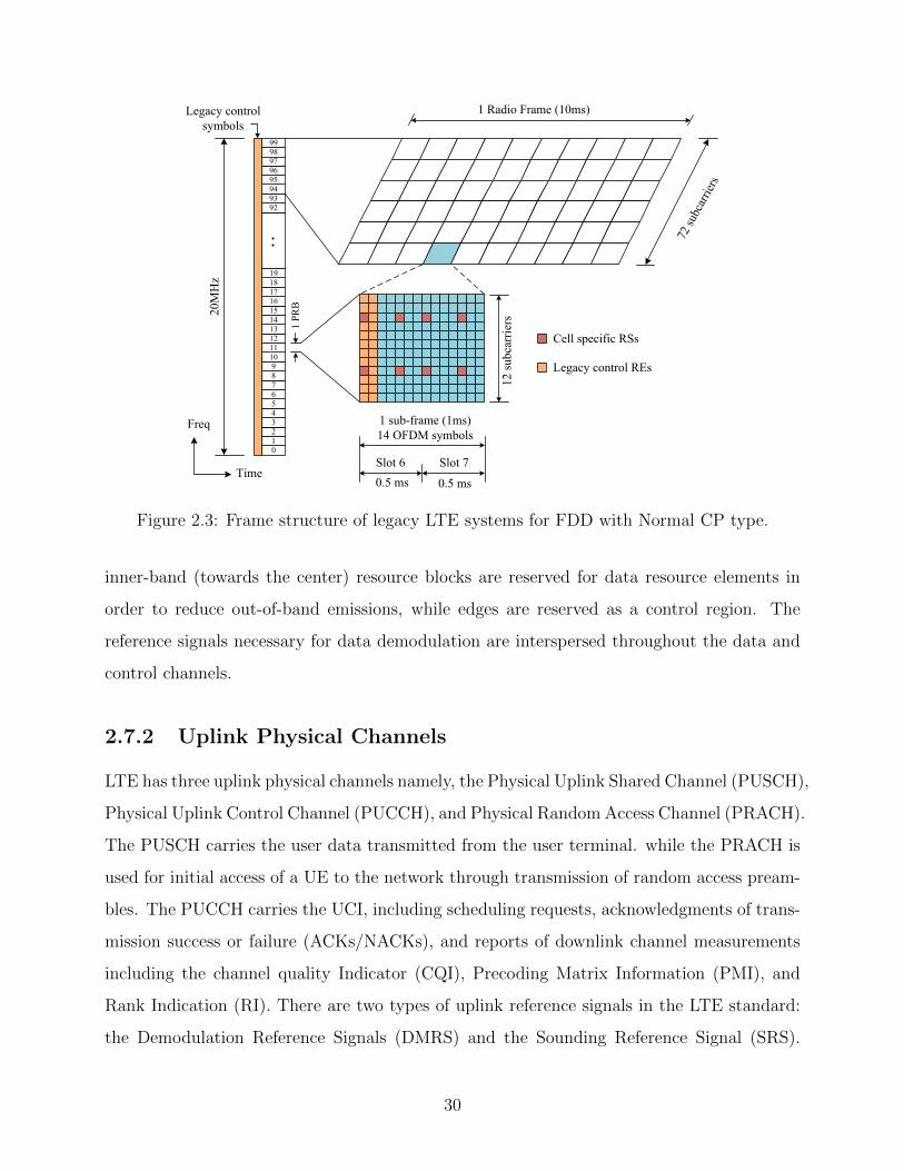
1 P
RB
20
MH
z
0123456789
10111213141516171819
9293949596979899
Legacy control
symbols
1 sub-frame (1ms)
14 OFDM symbols
12
su
bca
rrie
rs
Slot 6 Slot 7
0.5 ms 0.5 ms
Cell specific RSs
Legacy control REs
Time
Freq
1 Radio Frame (10ms)
72 s
ubca
rrie
rs
Figure 2.3: Frame structure of legacy LTE systems for FDD with Normal CP type.
inner-band (towards the center) resource blocks are reserved for data resource elements in
order to reduce out-of-band emissions, while edges are reserved as a control region. The
reference signals necessary for data demodulation are interspersed throughout the data and
control channels.
2.7.2 Uplink Physical Channels
LTE has three uplink physical channels namely, the Physical Uplink Shared Channel (PUSCH),
Physical Uplink Control Channel (PUCCH), and Physical Random Access Channel (PRACH).
The PUSCH carries the user data transmitted from the user terminal. while the PRACH is
used for initial access of a UE to the network through transmission of random access pream-
bles. The PUCCH carries the UCI, including scheduling requests, acknowledgments of trans-
mission success or failure (ACKs/NACKs), and reports of downlink channel measurements
including the channel quality Indicator (CQI), Precoding Matrix Information (PMI), and
Rank Indication (RI). There are two types of uplink reference signals in the LTE standard:
the Demodulation Reference Signals (DMRS) and the Sounding Reference Signal (SRS).
30

Both uplink reference signals are based on Zadoff-Chu sequences [82].
Zadoff-Chu sequences are also used in generating downlink Primary Synchronization Sig-
nals (PSSs) and uplink preambles. Reference signals for different UEs are derived from
different cyclic shift parameters of the base sequence.
2.7.2.1 Demodulation Reference Signals (DMRS)
DMRSs are transmitted by UE as part of the uplink resource grid. They are used by the
uplink channel estimation to equalize and demodulate the uplink control (PUCCH) and data
(PUSCH) information. In the case of PUSCH, when a normal cyclic prefix is used, DMRS
signals are located on the fourth OFDM symbol of each slot and extend across all the resource
blocks. In the case of PUCCH, the location of DMRS will depend on the format of the control
channel.
2.7.2.2 Sounding Reference Signals (SRS)
SRSs are transmitted on the uplink in order to enable the base station to estimate the up-
link channel response at different frequencies. These channel-state estimates may be used
for uplink channel-dependent scheduling. This means the scheduler can allocate user data
to portions of the uplink bandwidth where the channel responses are favorable. SRS trans-
missions are used for timing estimation and control of downlink channel conditions when
downlink and uplink channels are reciprocal or identical (TDD mode).
2.7.2.3 Physical Uplink Control Channel (PUCCH)
The PUCCH carries three types of control signaling information: ACK/NACK signals for
downlink transmission, scheduling requests (SR) indicator sent by UE when it intends to
transmit uplink data on PUSCH, and finally the feedback from the downlink channel in-
formation, including the Channel Quality Indicator (CQI), the Precoding Matrix Indicator
(PMI), and the Rank Indicator (RI). The last three indicators are representing the chan-
nel state information (CSI). Furthermore, the feedback of the downlink channel information
relates to MIMO modes in downlink. In order to ensure the correct choice of the MIMO
transmission schemes in downlink, each terminal must perform measurements on the quality
31

of the radio link and report the channel characteristic to the base station. This essentially
describes the channel quality functions of the UCI as contained in the PUCCH.
2.7.2.4 Physical Random Access Channel (PRACH)
If a UE would like to transmit on the PUSCH but does not have resource on this channel,
it should send a scheduling request on the PUCCH. However, in order to initiate access
to the PUCCH, the UE shall initiate the random access procedure. It uses the Physical
Random Access Channel (PRACH) to transmit a preamble to begin such procedure. Since
this corresponds to the first communication from the UE to the base station, the system
does not know the type or specifications of the UE device. After exchanging messages with
the UE, the base-station sends the resource grants on the PUSCH and the required time-
advance. Various transmission modes, such as Cyclic Delay Diversity (CDD) and Precoding
Vector Switching (PVS), provide a transparent way of decoding the preamble information.
The PRACH is transmitted on six RBs for the duration up to one subframe long. The exact
length and the frequency offset of the PRACH is advertised by the base station using System
Information Block-Type 2 (SIB2). A PRACH transmission has a cyclic prefix, a preamble,
and a guard period. The preamble sequences have one or two symbols of 800 microseconds,
and are generated from Zadoff-Chu sequences. The guard period is used to prevent collisions
of the symbols at the base station as the PRACH is sent without timing advance. The
preamble format defines the time duration of each field. There are three formats depending
on the size of the cell and the signal strength.
2.7.2.5 Physical Uplink Shared Channel (PUSCH)
When the UE receives an uplink scheduling grant, the PUSCH carries uplink user data and
signalling transport blocks arriving from the MAC layer to the physical layer. The UE sends
one transport block at a time, where CRC is attached to it to help the base station in the error
detection process. The resulting block is turbo coded with rate 1/3 and sent through rate
matching. Then the UE reassembles the coded transport blocks in the form of codewords,
where codewords from the data block are multiplexed with the control signals. Following
this process, the transport block is passed to the physical processor where each codeword is
32

scrambled and the modulation mapper groups the codeword bits into modulation symbols.
These modulated symbols go through a forward Fast Fourier Transform (FFT), then mapped
to the physical resources using the resource element mapper. Finally, time domain uplink
signal is generated using SC-FDMA. On the resource grid, the PUSCH occupies a contiguous
set of resource blocks around the center of the uplink band, and the edges of the band are
reserved for the PUCCH. Each subframe contains six PUSCH symbols and one demodulation
reference symbol.
2.7.3 Downlink Physical Channels and Functionalities
The Legacy LTE has a single type of traffic logical channel which is the Dedicated Traffic
Channel (DTCH), and four types of control logical channels: the Broadcast Control Chan-
nel (BCCH), the Paging Control Channel (PCCH), the Common Control Channel (CCCH),
and the Dedicated Control Channel (DCCH). The dedicated logical traffic channel and all
the logical control channels, except for PCCH, are multiplexed to form a transport channel
known as the Downlink Shared Channel. The Paging Control Channel (PCCH) is mapped to
the Paging Channel (PCH) and combined with the DL-SCH to form the Physical Downlink
Shared Channel (PDSCH). The PDSCH and four other physical channels (PDCCH, Physical
Downlink Control Channel; PHICH, Physical Hybrid Automatic Repeat Request Indicator
Channel; PCFICH, Physical Control Format Indicator Channel; and PBCH, Physical Broad-
cast Channel) provide all the user data, control information, and system information needed
in the unicast mode, which are delivered from higher layers.
2.7.3.1 Reference Signals
Downlink reference signals support the channel estimation functionality needed to equalize
and demodulate the control and data information. They are used in CSI measurements
(such as RI, CQI, and PMI) needed for channel quality feedback. LTE specifies five types of
reference signal for downlink transmission, namely: Cell-Specific Reference Signals (CSR),
UE-Specific Reference Signals, Channel-State Information Reference Signal (CSI-RS), MBMS
reference signals, and Positioning reference signals. MBMS reference signals are used in the
coherent demodulation employed in multicast/broadcast services, and the positioning refer-
33

ence signal is first introduced in R9 to provide measurements on multiple cells helping in
estimating the position of a given terminal.
Cell-Specific Reference Signals
Cell-Specific Reference Signals (CSRs) are common to all users in a certain cell, and are
transmitted in every downlink subframe and in every resource block in the frequency domain,
thus cover the entire cell bandwidth. The CRSs can be used by the terminal for channel
estimation for coherent demodulation of any downlink physical channel except PMCH and
PDSCH in the case of transmission modes 7, 8, or 9, corresponding to non-codebook-based
precoding. The CRSs can also be used by the UE to acquire CSI. Also the UE measurements
such as CQI, RI, and PMI performed on CRSs are used as the basis for cell selection and
handover decisions.
UE-Specific Reference Signals
UE-specific reference signals, also known as demodulation reference signals (DMRS), are
only used in downlink transmission (modes 7, 8, or 9), where CSRs are not used for channel
estimation. DMRSs first introduced in LTE R8 in order to support a single layer, and later
in R9 to support up to two layers. Furthermore, an extended specification introduced in R10
aimed to support up to eight simultaneous reference signals.
When only one DMRS is used, 12 reference symbols are inserted in resource blocks pair.
CSRs require spectral nulls or unused resource elements on all other antenna ports when a
resource element on any given antenna is transmitting a reference signal. This is a major
difference between CSR and DMRS. When two DMRSs are used on two antennas, all 12
reference symbols are transmitted on both antenna ports. The interference between the
reference signals is mitigated by generating mutually orthogonal patterns for each pair of
consecutive reference symbols.
CSI Reference Signals CSI-RSs are designed for cases where we have between four and
eight antennas. CSI-RSs were first introduced in LTE R10. They are designed to perform
a complementary function to the DMRS in LTE transmission mode 9. While the DMRS
supports channel estimation functionality, a CSI-RS acquires CSI. To reduce the overhead
resulting from having two types of reference signal within the resource grid, the temporal
34

resolution of CSI-RSs is reduced. This makes the system incapable of tracking rapid changes
in the channel condition. Since CSI-RSs are only used with four to eight MIMO antenna
configurations, and this configuration is only active with low mobility, the low temporal
resolution of CSI-RSs does not pose a problem.
2.7.3.2 Synchronization Signals
In addition to reference signals, LTE also defines synchronization signals. Downlink syn-
chronization signals are used in a variety of procedures, including the detection of frame
boundaries, determination of the number of antennas, initial cell search, neighbor cell search,
and handover. Two synchronization signals are available in the LTE: the Primary Syn-
chronization Signal (PSS) and the Secondary Synchronization Signal (SSS). Synchronization
signals are related to the PHY cell identity. There are 504 cell identities defined in the LTE,
organized into 168 groups, each of which contains three unique identities. The PSS carries
the unique identities 0, 1, or 2, whereas the SSS carries the group identity with values 0 to
167. Thus the physical layer cell identity NcellID = 3N1
ID +N2ID is uniquely defined by a number
N1ID in the range of 0 to 167, representing the cell ID group, and a number N2
ID in the range of
0 to 2, representing the sector ID within the group. Both the PSS and the SSS are mapped
onto the central 62 subcarriers with another 10 subcarriers on the boundaries padded with
zeros, forming the central 6 RBs (72 subcarriers located around the DC subcarrier). Using
this structure, a UE can receive both synchronization signals without prior knowledge of the
downlink bandwidth. In an FDD frame, they are positioned in subframes 0 and 5, next to
each other with the PSS and the SSS placed in the last two OFDM symbols of slots 0 and 10
respectively. The PSS determines one of the three possible values of the cell identity within
a group. To do so, each cell ID uses one of three Zadoff-Chu root sequences of length 63.
The process of the PSS is done by 5 ms monitoring and comparing it to find the used root
sequence making use of the good cross-correlation properties of the Zadoff-Chu sequences.
Hence, the UE can measure the time at which the PSS arrived and extract a cell identify
within a group. Then, the UE uses this timing information to receive the SSS which uses
an interleaved concatenation of two binary m-sequences, each of length 31 known as Gold
sequences to identify the cell group. The combination of these two sequences differs between
35

subframes 0 and 5. The concatenated sequence is scrambled with a scrambling sequence
given by the primary synchronization signal. Using cross correlation, the UE will be able to
identify the CP type (Normal or extended) and the duplex mode (FDD or TDD) as well as
exact timing within the frame.
2.7.3.3 Physical Downlink Broadcast Channel (PBCH)
The PBCH carries the Master Information Block (MIB), which contains the basic physical
system information and cell-specific information needed during the cell search. After the
mobile terminal correctly acquires the MIB, it can then read the downlink control and data
channels and perform necessary operations to access the system. The MIB contains four fields
of information. The first two fields hold information regarding downlink system bandwidth
and PHICH configuration. The downlink system bandwidth is communicated as one of six
values for the number of resource blocks in downlink (6, 15, 25, 50, 75, or 100). Those values
for the number of resource blocks map directly to bandwidths of 1.4, 3, 5, 10, 15, and 20
MHz, respectively. The PHICH configuration field of the MIB specifies the duration and
amount of the PHICH. The PBCH is always confined to the first four OFDM symbols found
in the first slot of the first subframe of every radio frame. The base station maps the MIB
on the PBCH across 40 ms periods (four radio frames), with portions transmitted in the first
subframe of every frame. When using normal CP, the PBCH occupies 72 subcarriers (6 RBs)
centered on the DC subcarrier using the first four symbols of slot one.
The data of the broadcast channel arrives to the coding unit in the form of a maximum
of one transport block every transmission time interval of 40 ms. Generally there are 14
information bits plus 10 spare bits (set to all zeroes currently), makes total 24 bits. From
these information bits, 16 CRC parity bits are computed. The eNodeB can use 1, 2 or 4
antennas for transmission. The CRC bits are scrambled based on the 1, 2 or 4 antenna used
in the transmitter. Hence, the total number of bits becomes 14 + 10 + 16 = 40 bits. After
the convolutional encoder, the total number of bits (for normal CP) becomes = 40×3 = 120.
Then, 24× 3 NULLs are appended to these 120 bits to make 192 for sub-block interleaving
and inter-column permutations. These bits are repeated 16 times by discarding the appended
Nulls resulting in 120 × 16 = 1920 bits (or 1728 bits in case of Extended CP), then QPSK
36

mapped so that the total number of QPSK symbols becomes = 1920/2 = 960 symbols (or
864 symbols in case of Extended CP). These 960 symbols are segmented into four equal
sized self-decodable units or segments. These symbols are then placed in PBCH Resource
Elements in the second slot of the first subframe (slot 1). That is the first subframe’s second
slot contains 960/4 = 240 symbols (or 216 symbols in case of Extended CP) and then inserted
in the OFDM resource elements. PBCH is restricted to the 72 subcarriers around the DC
in the resource grid irrespective of the UE bandwidth. The PBCH is transmitted in the
first four OFDM symbols of the second slot of the first subframe in every radio frame. For
example, in a subframe which contains PBCH (e.g. first subframe of a frame) there are total
72 × 7 × 2 = 1008 REs (for normal CP). Out of that, currently in that subframe, the total
number of CRS (Cell Reference Signal) = (4× 6)× 6= 144 REs (for 4-antennas system). If
the system is using single antenna instead of 4 antennas, then 48 REs will be having CRSs
and the remaining elements (out of 144) will be Null.
2.7.3.4 Physical Downlink Control Format Indicator Channel (PDCFICH)
The PDCFICH is used to define the number of OFDM symbols that carry the Downlink
Control Information (DCI) in a subframe. The PDCFICH information is mapped to specific
resource elements belonging to the first OFDM symbol in each subframe. The possible val-
ues for PDCFICH (one, two, three, or four) depend on the bandwidth, frame structure, and
subframe index. For the 1.4 MHz bandwidth, since the number of resource blocks is quite
small, PDCFICH may need up to four symbols for control signaling. However, for the larger
bandwidths, the number can take up to three OFDM symbols.
2.7.3.5 Physical Downlink Control Channel (PDCCH)
In order to start communication between the base station and the mobile terminal (UE), a
PDCCH is defined for each Physical Downlink Shared Channel (PDSCH) channel. PDCCH
mainly contains the scheduling decisions that each terminal requires in order to successfully
receive, equalize, demodulate, and decode the data packets. Since the PDCCH information
must be read and decoded before decoding of PDSCH begins, in a downlink PDCCH occupies
37

the first few OFDM symbols of each subframe. The exact number of OFDM symbols at the
beginning of each subframe occupied by the PDCCH (typically one, two, three, or four)
depends on various factors, including the bandwidth, the subframe index, and the use of
unicast or multicast services.
The control information carried on the PDCCH is known as Downlink Control Information
(DCI). Depending on the format of the DCI, the number of resource elements (i.e., the number
of OFDM symbols needed to carry them) varies. There are 10 different possible DCI formats
specified by the LTE standard (known as 0,1,1A,1B,1C,1D,2,2A,2B,2C,2D,3,3A,4), with each
format contains a specific set of information and certain purpose. The information carried
by DCI format are: resource allocation information, such as resource block size and resource
assignment duration; transport information, such as multi-antenna configuration, modulation
type, coding rate, and transport block payload size; and information related to the HARQ,
including its process number, the redundancy version, and the indicator signaling availability
of new data. The scheduling messages transmitted over the PDCCH are addressed to a certain
Radio Network Temporary Identifier (RNTI). A variety of RNTI types are used in LTE to
define the identity of the intended UE which should read the scheduling messages, and the
type of these messages. The type of the RNTI is used to generate the CRC code that will
be used by the transport layer to encode the DCI information.
The resource element mapping of the PDCCH is done using control channel elements
(CCE), each contains 9 resource element groups (REG). Each REG consists of 4 REs. Based
on the length of the DCI message, the base station maps the PDCCH onto 1,2,4 or 8 consec-
utive CCE. This is called the aggregation level. In other words, based on the length of the
DCI, PDCCH can be scheduled onto 36, 72, 144, or 288 resource elements.
Further, the CCEs are organized into common search spaces and UE-specific search spaces.
The first type is available to all UE in the cell and have predefined location in the downlink
region. However, the second type is assigned to groups of UEs and its location depends on
the RNTI type of the UE.
As the aggregation level of a UE changes from a subframe to another, and the length
of DCI changes the aggregation level, the UE locates its PDCCH and find the DCI format
using blind detection. In other words, a UE attempts to decode using all DCI formats with
38

candidate locations in the search space, and the correct combination is the one that checks the
CRC. The reliability of the PDCCH is enhanced by means of transmit diversity using space-
frequency block codes, and is protected against inter-cell interference using a cell-specific
scrambling pattern.
Although the described PDCCH functions work fine for most of the situations, it suffers
from some limitations as the requirements of the LTE network evolves. First, limiting the
channel resources to the first 3-4 symbols of slot 0 has a direct limitation on the cell capacity
(number of users could be scheduled). Second, PDCCH is transmitted only in a distributed
manner, hence, it cannot benefit from the beamforming using MIMO while the base station
enjoys multiple antennas. Third, with the PDCCH transmissions of a certain user spread
over the entire frequency band, it does not benefit form frequency selective scheduling nor
inter-cell interference coordination.
The aforementioned reasons urged the evolution towards the Enhanced Physical Down-
link Control Channel (EPDCCH) in R11. The EPDCCH still carries the same information of
PDCCH except that it shares the resources with the traffic PDSCH to increase the capacity.
Within each subframe, a resource block pair is either assigned to PDSCH or EPDCCH, which
makes the capacity of the new control channel adjustable and also makes use of interference
coordination. EPDCCH is transmitted on newly defined four antenna ports (AP 107 - 110),
which are associated with the reference signals (occupying the same REs as AP 7-10). EPD-
CCH and its reference signals are preceded with a user-specific preceding matrix, and also
supports multiuser MIMO (MU-MIMO)with up to 4 layers (i.e. supporting simultaneously
4 different users).
2.7.3.6 Physical Downlink Shared Channel (PDSCH)
After the base station sends the UE a scheduling command, it transmits the data of the DL-
SCH using the scheduling commands defined. The PDSCH carries downlink user data and
signalling transport blocks arriving from the MAC layer to the PHY. Specifically, transport
blocks are transmitted one at a time in each subframe. The base station adds 24-bit CRC
to each DL-SCH transport block which is used by the UE for error detection. Following
adaptive modulation and coding, the modulated symbols are mapped onto multiple time-
39

frequency resource grids, which are eventually mapped to multiple transmit antennas for
transmission. The type of MIMO technique used in each subframe can be adapted based on
the received SNIR (which indicates the channel conditions). It should be mentioned that,
the PDSCH and the PUSCH are the only physical channels that can adapt their modulation
scheme according to channel quality observed at the mobile terminal. The measurements
made at the terminal must be sent back to the base station in order to help the scheduling
decisions. At each subframe, the mobile terminal needs to be notified about the scheduling
from the base station for each transmitted resource block. Among the information that must
be communicated; are the number of resource blocks allocated to a user, the transport block
size, the type of modulation, the coding rate, and the type of MIMO mode used per each
subframe.
2.8 Physical Layer Features for LTE-MTC Systems
The behaviour of the MTC terminals is different from the legacy LTE users, for which the
LTE was optimized. Therefore, in order to accommodate the new requirements, the CAT-M
UE category is recently added for MTC communication in R13. A lot of effort was put to
specify a new UE for MTC operation in LTE which allows for enhanced coverage compared
to existing LTE networks and low power consumption. In details, the LTE-MTC specifies
a new R13 low complexity UE category for MTC operation in LTE half duplex FDD mode
based on the R12 low complexity UE category supporting additional capabilities. Among
these capabilities, is a reduced UE bandwidth of 1.4 MHz for the downlink and uplink with
the ability to operate within any system bandwidth. Also, the frequency multiplexing of
bandwidth reduced UEs and non-MTC UEs should be accommodated. For the new UE
category to have a tangible complexity reduction, the maximum transmit power of the new
UE power should be reduced such that an integrated power amplifier (PA) implementation
is possible. Also, power consumption reduction is a must for the LTE-MTC UE target ultra-
long battery life. The most important feature of the new category, is to improve the LTE
coverage corresponding to almost 15 dB for FDD.
A variety of techniques is considered to achieve such requirements, including: subframe
40

bundling techniques with HARQ for physical data channels (PDSCH, PUSCH), repetition
techniques for control channels (e.g. PBCH, PRACH, EPDCCH), uplink Power Spectral
Density (PSD) boosting with smaller granularity than 1 PRB, resource allocation using
EPDCCH with cross-subframe scheduling and repetition, new physical channel formats with
repetition for SIB/RAR/Paging, new SIB for bandwidth reduced and coverage enhanced
UEs, and increased reference symbol density and frequency hopping techniques.
2.8.1 MTC Features
More constrains are added on the MTC UE to reduce its cost and complexity. The features
of the physical downlink control channel for MTC are summarized as:
• The design of the physical downlink control channel for MTC is based on EPDCCH.
• The introduction of new DCI messages to R13 for low complexity UEs.
• The use of a narrowband (within 6 PRBs) control channel.
• Its usage for other UEs in enhanced coverage.
• The demodulation of the control channel shall be based on CRS and/or DMRS.
2.8.1.1 Modes Of Operation
In Rel-13, the CAT-M UE is referred to as Bandwidth-reduced Low-complexity and Coverage
Extension user equipments (BL/CE UE). BL/CE UEs can operate in two different modes
of operation: CE Mode A and CE Mode B, each depends on the coverage extension level
seen by the UE. The operation mode is determined by the eNodeB and sent to the UE with
radio resource control message. The UE selects one of 4 different CE levels, namely level
1,2,3 and 4, based on the reference signal received power. Each level is distinguished by a
different random access channel configuration and the time and frequency resources used by
the UE for the random access transmissions. For CE Mode A, associated with CE level 1
and 2, a UE would have an equivalent coverage as that of UE CAT-0. This mode requires
small number of repetition of different channels, or in the best case no repetitions at all.
41

Also, the power control mechanism used for Mode A is the same as the legacy users. For the
repeated transmissions, the used transmit power remains unchanged during the repetition
period. For CE Mode B, the UE is in CE level 3 or 4, and is covered with extended coverage
of 15 dB with reference to CAT-0 (equivalent to 155.7 dB Maximum Coupling Loss (MCL)
between the transmitter and the receiver). CE Mode B features a medium or large number of
repetitions, and the transmission power of the uplink channels is set to the maximum value.
Hence, no power control is needed, which makes the control information sent to this category
has a unique format as well.
2.8.1.2 Narrowband Concept
The bandwidth choice of a certain base station is configured once and remains unchanged
during operation, hance, it would be a good choice to use a bandwidth unit that can be
a common divisor of the available bandwidth options in the legacy LTE. Then the choices
become limited to 6 RBs or one RB. However, in order for the MTC devices to capture the
signature of the LTE signal, it will have to receive the synchronization signals PSS and SSS.
These signals occupy the central 6 RBs of the bandwidth of the base station, which makes it
desirable for the MTC devices to take 6 RBs as the basic unit of bandwidth. Not only that,
but also as mentioned before, the legacy PDCCH is mapped to the full occupied bandwidth,
which makes decoding PDCCH is not possible in MTC applications, since the UE is limited
to bandwidth of only 1.4 MHz. However, the enhanced version EPDCCH, uses one PRB pair
as the basic resource unit, which makes it a good candidate to be used to control MTC UE.
Furthermore, the use of only one PRB for the MTC control channels based on EPDCCH was
reported to be insufficient, as it could provide the required converge enhancement (CE) [83].
It was concluded in [84] that, increasing the bandwidth of the basic EPDCCH to 6 PRBs
in the 1.4 MHz bandwidth on the MTC UE along with repetition will be sufficient to have a
good coverage of -14 dB. Furthermore, coverage enhancement can be achieved by employing
EPDCCH that supports beamforming which increases coverage by directing the power of
the base station towards the UE. For these reasons, it is agreed on to use the 6RBs (or one
narrowband (NB)) as the basic bandwidth unit for MTC. A narrowband is defined as six
non-overlapping consecutive physical resource blocks in the frequency domain. The total
42

NBn
NBn+1
NBn+2
NBn-1
NBn-2
Slot
# 0
Slot
# 1
Slot
# 10
Slot
# 11
Slot
# 18
Slot
# 19
Sub-frame
# 0Sub-frame
# 5
Sub-frame
# 9
1 PRB
0.5ms
1 ms
PSS
Symbol
SSS
SymbolF
req.
Time
Figure 2.4: Frame structure of LTE-MTC systems for FDD with Normal CP type showing
the synchronization signals. The concept of narrowband is highlighted.
number of downlink narrowbands in the downlink transmission bandwidth configured in the
cell is given by NDLNB = ⌈N
DLRB
6⌋ and are numbered nNB = 0, ..., NDL
NB − 1 in order of increasing
physical resource-block number. The narrowband concept and numbering is highlighted in
Fig. 2.4.
2.8.1.3 Frequency Hopping
With the small bandwidth offered to MTC UE and the use of single receiver chain, the fre-
quency and spatial diversity are taken away. To retrieve some of the lost frequency diversity,
the frequency hopping concept is added to the MTC LTE system. In other words, MTC
transmissions will hop from one NB to another to make use of transmitting over different
channels. Hence, providing frequency diversity. However, frequency hopping shall introduce
new challenges due to the fact that the UE will have to re-tune its RF chain every time it
hops. The re-tuning consumes some time and might affect the overall behaviour. Therefore a
guard period is needed for re-tuning. Rel-13 specifies the re-tuning guard period as the time
duration of two orthogonal frequency division multiplexing (OFDM) symbols. No transmis-
sion or reception is done by the UE during the guard period. The time of the guard period
varies depending on whether it is downlink or uplink.
43

2.8.1.4 Repetitions
As mentioned before, the limitations forced on the MTC LTE directly affects the downlink
control channel, which in turn, has a direct impact on the performance of the downlink. For
the downlink to have sufficient link budget to support the prospected coverage enhancement,
an enhanced version of the distributed EPDCCH is reused as the base control signal for MTC.
Thus, enhancement is obtained by transiting repeated copies of the same signal over time.
As a direct result of the use of such repetition code, the link performance can be enhanced
through time diversity and boost the control signal energy. On the other hand, the repetition
has the effect of increased decoding time (more latency), which requires more wake-up time
of the MTC device. The maximum number of repetitions for different physical channels and
signals is given in Table 2.2.
Table 2.2: Maximum number of repetitions for different channels.
CAT-M Channel Mode A Repetitions Mode B Repetitions
PSS/SSS 1 1
PBCH 1 5
MPDCCH 16 256
PDSCH 32 2048
PUSCH 32 2048
PUCCH 8 32
PRACH 32 128
2.8.2 MTC Physical Random Access Channel (MPRACH)
The legacy design of the PRACH channel is limited to 6 RBs only, which makes it suitable for
the MTC use as it signifies the narrowband constraint. However, the legacy PRACH needs
some modifications to support the extra path-loss due to the extended coverage. Hence,
repetitions and frequency hopping are exploited to provide the necessary diversity to the
MPRACH. Like the legacy PRACH, The physical layer random access preamble consists of
44

a cyclic prefix of length TCP and a sequence part of length TSEQ with different 5 preamble
formats (0,1,2,3,4). The values of these parameters depend on the frame structure and the
random access configuration and the preamble format is controlled by higher layers. For
each coverage enhancement level, UEs with different geographic locations may have different
radio conditions and propagation delay. Thus, different PRACH repetition levels could apply
to different preamble formats to adapt to different propagation delay and compensate for
different propagation losses. For each PRACH coverage enhancement level, there is a PRACH
configuration done at higher layers with a PRACH configuration index values from 0 to 63,
a PRACH frequency offset, and a number of PRACH repetitions per attempt NPRACHrep . The
UE selects the repetition level to use for the initial transmission based on DL measurements,
but this is only acceptable if sufficient DL measurement accuracy can be achieved within
a reasonable DL measurement time. If sufficient accuracy cannot be achieved, the UE will
start at the lowest configured PRACH repetition level. The number of repetitions as well as
the starting subframe are also configured by higher layer signalling. It has been proposed
that, the UE should remember what PRACH repetition level is used last time and use this
information when setting the starting point for the next access. PRACH frequency hopping
may provide frequency diversity gain and reduce the number of repetition. From this point
of view, the power consumption of enhanced PRACH transmission could be saved due to
reduced active time.
2.8.3 MTC Physical Downlink Control Channel (MPDCCH)
EPDCCH has been chosen to be the starting point towards designing the new MTC control
channel MPDCCH. However, special requirements have been adapted to best suite the new
MTC platform and to support the required coverage with reasonable complexity and power
consumption. The new set of features for MPDCCH require defining new set of downlink
control formats, adding a possibility for a common UE to access the control channel by
introducing the new common search space, and enhancing the control channel assignment
procedure to support the new MTC features such as repetition and frequency hopping. A
summary of the introduced features to design the new MPDCCH is shown in Fig. 2.5.
45

MPDCCH
MPDCCH
Assignment
Aggregation Types
PRB Sets
Repetition
Localized
Distributed
1 Set
(2 or 4 PRBs)
2 Sets
(2+4 PRBs)
Aggregation Levels
Frequency Hopping
Search Spaces
(SS)
UE Specific Search
Space (SSS)
Common Search
Space (CSS)
Type-0 CSS
Type-1 CSS
Type-2 CSS
DCI Formats
Format 6-0
Format 6-1
Format 6-2
Format 6-0A
Format 6-0B
Format 6-1A
Format 6-1B
Figure 2.5: Summary for the introduced features for MPDCCH.
2.8.3.1 MTC Search Spaces
In LTE systems, the downlink control region is shared by all UEs in one cell. Each UE
should monitor the control region and perform blind decoding to detect whether or not there
is control information for itself. In order to reduce the number of blind decoding trials per
UE, each UE has a defined search space area of the control region to monitor, rather than
having to monitor the whole control region. The search space is defined on the basis of
enhanced control channel elements (ECCEs). Control information may occupy 1, 2, 4, or 8
CCEs aggregated together depending on the size of the control information and the channel
quality of the UE.
The search space starting point for a UE is determined by a hash function and the search
space size is determined by the PDCCH aggregation level. The hash function randomizes the
search space locations of different UEs and effectively reduces the blocking probability. The
MPDCCH has two broad classes of search spaces: UE-specific search space (USS) for messages
directed specifically to the UE and Common Search Space (CSS) for messages directed to
multiple users or for messages to a specific UE before the USS has been configured. It is
46

worth to mention that the legacy EPDCCH has only USS since PDCCH is used for the CSS.
In MPDCCH, the UE will have to blindly decode both USS and CSS. The search spaces will
differ depending on the CE mode whether mode A or mode B.
2.8.3.2 MTC DCI Formats
Generally, the eNodeB employs the downlink control information messages to send down-
link scheduling commands, uplink scheduling grants, and uplink power control commands
to the UE. The DCI can be written using several different formats. Indeed, conventional
LTE-A systems up to R12 support 14 different formats, namely format 0, 1/1A/1B/1C/1D,
2/2A/2B/2C, 3/3A, 4, and 5. Each format contains a specific set of information and has
a specific purpose. However, some formats have been grouped under common name which
implies that the main functionality of these downlink messages would have something in
common but the details will be different. For instance, the main theme for Format 1 and
its group is to mainly provide the downlink scheduling information such as the PRB alloca-
tion, modulation and coding, and single or multiple users support. The differences from one
format to another in the same group are to which transmission mode and antenna system
to use. Also, the basic purpose for Format 2 is to set configuration for MIMO systems.
However, they differ on how the MIMO system is configured on being used for open loop,
closed loop, beamforming, and multi-user MIMO configurations. Although there have been
multiple formats to send various scheduling commands, in LTE-MTC systems, new formats
have been introduced to the system. The motivation is to skip the unused parameters such
as the number of codewords since LTE-MTC is defined for a single codeword. Also, the DCI
messages for both uplink and downlink grants were designed to fit the same number of bits
with some indication bits to differentiate between the formats. This is mainly to reduce the
blind decoding iterations and hence, reduced UE complexity. Furthermore, with the intro-
duction of enhanced coverage, repetition, and frequency hopping, the UE will mainly require
new information to facilitate the use of repetition, narrowband resource assignment, fre-
quency hopping flag. For example, downlink DCI assignment should indicate the MPDCCH
repetition factor so that UE can expect when the message is complete. For these reasons
and others, three new DCI formats, namely format 6-0, 6-1, and 6-2 have been defined for
47

LTE-MTC system for uplink grant, downlink scheduling, and paging, respectively. To best
suite the operating mode, whether being Mode A or Mode B, there are two versions for each
format where the number of information bits differ.
2.9 Physical Layer Features for NB-IoT Systems
2.9.1 Deployment Scenarios and Modes of Operation
As a finite and scarce natural resource, spectrum needs to be used as efficiently as possible.
Thus, technologies that use spectrum tend to be designed to minimize usage [85]. To achieve
spectrum efficiency, NB-IoT has been designed with a number of deployment options for
GSM, WCDMA, or LTE spectrum. There are three deployment scenarios.
1. In-band Operation: An NB-IoT carrier is a self-contained network element that uses
a single PRB. For in-band deployments with no IoT traffic present, the PRB can be
used by LTE for other purposes, as the infrastructure and spectrum usage of LTE and
NB-IoT are fully integrated. The base station scheduler multiplexes NB-IoT and LTE
traffic onto the same spectrum, which minimizes the total cost of operation for IoT
services. To support full flexible design, the specifications define two modes for the
in-band operation. The first mode, namely Same-PCI mode, assumes that the NB-IoT
carrier has identical cell parameters (i.e., cell ID and number of Tx antennas) as the
donor legacy cell. The other mode considers some flexibility of having a different cell
ID and different number of Tx antennas.
2. Stand-alone Operation: This mode of operation is mainly intended to replace a
GSM carrier with an NB-IoT carrier. By steering some GSM traffic to the WCDMA
or LTE network, one or more of the GSM carriers can be used to carry IoT traffic. As
GSM operates mainly in the 900 MHz and 1,800 MHz bands (spectrum that is present
in all markets), this approach accelerates time to market, and maximizes the benefits
of a global-scale infrastructure.
3. Guard band Operation: this can be applied either in WCDMA or LTE. To operate
48

in a guard band without causing interference, NB-IoT and LTE need to coexist. The
physical NB-IoT layer is designed with the requirements of LTE guard band coexistence
specifically taken into consideration. Again, NB-IoT uses OFDM in the downlink and
SC-FDMA in the uplink. The design of NB-IoT has fully adopted LTE numerology, us-
ing 15kHz subcarriers in the uplink and downlink, with an additional option for 3.75kHz
subcarriers in the uplink to provide capacity in signal-strength-limited scenarios.
It should be noted that, NB-IoT supports operation with only one or two Tx antenna
ports. For operation with two Tx antenna ports, NB-IoT uses the conventional Space Fre-
quency Block Coding (SFBC) employing the Alamouti mapping. Unlike other LTE-based
systems, NB-IoT utilizes the same transmission scheme for all physical channels including
Narrowband Physical Downlink Control Channel (NPDCCH), Narrowband Physical Broad-
cast Channel (NPBCH), and Narrowband Physical Downlink Shared Channel (NPDSCH).
2.9.2 Downlink Physical Channels
2.9.2.1 Frame Structure
With a carrier bandwidth of just 200KHz, an NB-IoT carrier can be deployed within an LTE
carrier as one PRB. Fig. 2.6 shows a 3MHz LTE carrier in which a single PRB is assigned to
NB-IoT. An operating NB-IoT band is defined as a contiguous set of 12 sub-carriers forming
one PRB. A single radio frame is 10ms which consists of 10 subframes with equal duration.
Each subframe is divided into two slots with equal periods. Unlike conventional LTE which
defines two CP types with different CP patterns, NB-IoT in R13 supports only the normal
CP type, where a slot is composed of 7 OFDM symbols. According to the specification [80],
if the signal is sampled at 1.92 MSamples/sec, similar to LTE-MTC, the CP length of the
first symbol in each slot is 10 samples and those of the other symbols are 9 samples long.
Also, in this case, the OFDM symbol spans N = 128 sub-carriers.
2.9.2.2 Synchronization Signals
NB-IoT intends to occupy a narrow bandwidth of only 200KHz, which is not backward com-
patible to the supported bandwidths by the legacy LTE. Therefore, NB-IoT redefines the
49

3M
Hz
0123456789
1011121314
Legacy control
symbols
12
su
bca
rrie
rs
Subframe #9
Slot #18S(131)
S(0)
Slot #19
S(11)
S(120)
1 sub-frame (1ms)
14 OFDM symbols
Subframe #5
P3(10)
P3(0)P13(0)
P13(10)1 sub-frame (1ms)
14 OFDM symbols
Subframe #0
1 sub-frame (1ms)
14 OFDM symbols
Subframe #1
NPSS Subframe NSSS SubframeNPBCH Subframe NPDCCH/NPDSCH
Subframe Inband CRS
NRS
Fre
q.
Time
Figure 2.6: Radio frame structure for NB-IoT systems. The allocated RB is expanded in
time to show the NPSS/NSSS symbols mapping in addition to the broadcast channel and
one data/control subframe.
cell attach procedure including cell search and initial synchronization [86] [85]. During initial
synchronization, CFO is estimated and compensated to enable proper signal detection. The
UE acquires the physical cell identification by employing the cell search procedure. To cope
with these changes, NB-IoT employs new set of synchronization signals, namely Narrowband
Primary Synchronization Signal (NPSS) and Narrowband Secondary Synchronization Sig-
nal (NSSS) [80]. The new sequences have different bandwidth, mapping, periodicity, and
generation when compared to the legacy LTE synchronization signals. Unlike conventional
LTE, cell ID is encapsulated only in the secondary sequence without involving the primary
sequence.
NPSS and NSSS sequences are constructed from a frequency domain Zadoff-Chu sequence
where NPSS length is 11 samples while the NSSS consists of 132 samples. The NPSS, Pl(n),
is generated such that Pl(k) = Q(l)e−jπuk(k+1)/11, where 0 ≤ k < 11, 3 ≤ l < 14 is the
OFDM symbol index, the sequence root u = 5, and Q(l) is a modulation sequence given by
1, 1, 1, 1,−1,−1, 1, 1, 1,−1, 1, respectively. In NB-IoT system, there are still 504 unique
physical cell IDs. However, all of them are only indicated by the NSSS. The NSSS, S(k), is
generated according to,
S(k) = Cq(k′) e−j2πθfk e−j
πuk(k+1)131 , 0 ≤ k < 132 (2.1)
where k′ = k mod 128, the root sequence, u, is related to the cell ID, NNcellID , by u = (NNcell
ID
mod 126)+3, and the cyclic shift, θf , is related to the System Frame Number (SFN), nf , such
50

that θf =31132
(nf/2) mod 4. The modulated sequence, Cq(k′), is given by Cq(k
′) = 2Cq(k′)−1,
where q is a cell specific parameter that is given by q = ⌊NNcellID /126⌋ and Cq forms four
complementary 128-bits binary sequences.
In conventional LTE, primary and secondary synchronization signals (i.e., PSS and SSS,
respectively) are mapped to two consecutive OFDM symbols in the same slot with a peri-
odicity of 5msec. However, NPSS is mapped to subframe 5 of every radio frame. NSSS is
mapped to the last 11 ODFM symbols of subframe 9 in radio frames having nf mod 2 = 0.
Sequences are mapped to frequency sub-carriers in an increasing order, then applied across
time as shown in Fig. 2.6.
2.9.2.3 Narrowband Reference Symbols (NRS)
Due to the lack of fully adoptable LTE signal structure in case of guard and stand-alone
modes, new reference signals or pilots, namely NRS, are inserted within the transmitted
signal to assist the channel estimation process which is required for coherent detection at
the UE side. Similar to legacy LTE, NRS uses a cell-specific frequency shift derived as the
modulo division of the NB-IoT cell ID by 6. The conventional LTE CRS sequence is reused
for NRS generation where the centre of LTE CRS sequence is employed as NRS sequence for
all PRBs. The NRS is mapped to the last two OFDM symbols of the slot for both antenna
ports in case of transmit diversity as shown in Fig. 2.6. As NPSS/NSSS occupy the last 11
OFDM symbols within the subframes transmitting NPSS/NSSS for normal CP, NRS are not
mapped to these subframes. To ensure the demodulation and/or measurement performance,
it has been agreed to transmit NRS in all valid subframes except the NPSS/NSSS subframes
regardless of whether there is downlink transmission in these valid subframes or not.
In in-band operation mode, the LTE CRS REs should be reserved from NB-IoT to avoid
pollution to the LTE channel estimation and measurement. However, as a special case,
NPBCH decoding shall not rely on LTE CRS due to the lack of knowledge of the legacy PRB
index information. This means that the new reference signal (i.e. NRS) alone should be able
to provide sufficient channel estimation performance for NPBCH decoding. The NPDCCH
and NPDSCH decoding performance can be ensured also based on NRS only. In this sense,
LTE CRS is not a must in-band operation mode in terms of DL channel decoding. However,
51

the standardization is designed to provide the flexibility to UE implementation for the use
of LTE CRS although the performance requirements do not rely on it. On the other hand,
the extra signalling overhead to support the use of LTE CRS would be limited since the
resource mapping information of the LTE CRS needs be anyhow indicated to realize the rate
matching around the LTE CRS REs. LTE CRS may also benefit measurement accuracy when
available. For these reasons, the specifications allow two modes for in-band operation. The
first assumes that the full information of the legacy cell in terms of the cell ID and number
of Tx antennas is identical to the NB-IoT carrier. In this case, the UE is free to utilize the
CRS for its own demodulation and/or measurements. On the other hand, the other mode
assumes that the UE is not aware of the legacy cell ID, but it has the information of the
number of its Tx antennas which helps determining the rate matching around the CRS.
2.9.2.4 Narrowband Physical Downlink Broadcast Channel (NPBCH)
Since NB-IoT has various deployment scenarios that require different system configurations,
some Narrowband Master Information Block (NB-MIB) fields are required to be operation
mode dependent. For example, the UE would require to puncture the CRS in case of in-band
operation. Therefore, a field representing the number of legacy Tx antennas is beneficial. In
the same mode, the PRB index is needed to validate the working assumption regarding the
potential usage of CRS for demodulation. In addition, there should be an indication for the
raster frequency offset for the in-band operation. It is understood that, during start, the UE
would scan the frequency spectrum searching for a valid NB-IoT carrier. In legacy LTE, the
raster frequency is assumed to be 100KHz starting from the center of the LTE band. However,
since the NB-IoT in-band deployment assumes that the NB-IoT carrier would be allocated
as a single PRB with 180KHz width, the raster frequency to the NB-IoT carrier would not
be multiples of 100KHz. Indeed, for odd LTE bandwidths, there is a frequency offset of
±7.5KHz for the raster frequency to be multiple of 100KHz. In fact, the synchronization
signal design and mapping are carefully studied so that a UE can lock to the NB-IoT carrier
with an ambiguity of ±7.5KHz. It is clear that a new field has to be added to the NB-MIB
in order to differentiate between the various frequency offsets as the bandwidth would not
be known.
52

In all cases, similar to LTE-MTC, NB-MIB indicates the scheduling information for the
system information messages by defining the TBS size and repetition filed for the first SIB
message (i.e., NB-SIB1). For these reasons, it was beneficial to design new NB-MIB fields
not only to include the introduced set of fields but also to interpret the fields depending on
the operation mode. The decision is to extend the NB-MIB length to 34 bits before CRC
attachment. This means that the code word for the broadcast channel becomes 150 bits
instead of only 120 bits. Furthermore, it was agreed that NPBCH consists of 8 independently
decodable blocks. Thus, after CRC attachment and channel coding, the NB-MIB is rate
matched to 1600 bits instead of 1200 bits for Normal CP type.
The rate matched bits are scrambled by the conventional LTE scrambler that is initialized
with the NB-IoT Physical Cell Identifier (PCI) in each radio frame fulfilling nf mod 64 = 0,
where nf is the SFN. This simply refers to the fact that a single NB-MIB transmission spans
64 radio frames. After the channel interleaver, the bits are QPSK modulated. The modulated
bits are mapped to resource elements in a frequency then time fashion. During the mapping,
the 800 QPSK modulated symbols are segmented into 8 consecutive segments such that each
segment is repeated in 8 consecutive radio frames. In other words, identical symbols carrying
the same segment are transmitted with 80ms duration. It is essential to enable the NPBCH
decoding without any prior information about the operation mode. Indeed, only cell ID and
proper frame timing are required through the conventional cell search procedure. Therefore,
it has been agreed that NB-PBCH is transmitted in subframe 0 in every radio frame, where
the first 3 symbols in a subframe are not utilized independent of the operational mode. In
addition, for rate matching purposes, the CRS are punctured assuming 4 Tx antenna ports
even for guard and stand-alone modes. Moreover, the number of NRS ports is considered
based on two transmit antennas independent of the actual configuration. However, the
number of NRS ports (i.e., whether 1 or 2) is indicated by NB-PBCH CRC masking similar
to the conventional system.
2.9.2.5 Narrowband Physical Downlink Control Channel (NPDCCH)
The NB-IoT has its own control channel with customized features and definitions. Although
some features have been adopted from LTE-MTC system, there are couple of restrictions that
53

NPDCCH
NPDCCH
Assignment
Repetition
Aggregation Levels
Search Spaces
(SS)
UE Specific Search
Space (SSS)
Common Search
Space (CSS)
Type-1 CSS
Type-2 CSS
DCI Formats
Format N0
Format N1
Format N2
Figure 2.7: Summary for the introduced features for NPDCCH.
mandates redefinitions for some of the control channel concepts. First of all, the NPDCCH
transmission becomes packet-based as the system only supports half-duplex mode at least for
R13 version. There is no overlapping between the data channel and the control channel within
the same subframe. The UE will monitor the NPDCCH when it expects a random access
response (RAR), a new DL assignment, paging, or uplink grant. In case of RAR or paging,
the UE has to monitor a common search space. Therefore, similar to LTE-MTC and unlike
the conventional EPDCCH, two search spaces have been defined for NB-IoT. Second, due to
the reduced set of information carried by the DCI messages, three new DCI formats, namely
N0, N1, and N2, have been defined only for NB-IoT in R13. Third, NPDCCH assignment
relies on repetition to support unconditional coverage enhancement with relatively small
aggregation levels again for complexity reduction. Fig. 2.7 shows the essential differences
between NPDCCH and other control channels in various LTE systems.
Two broad classes of search spaces have been defined for NB-IoT, namely USS for mes-
sages directed specifically to the UE and CSS for messages directed to multiple users, paging,
or for messages to a specific UE before the USS has been configured (i.e., RAR message).
Similar to LTE-MTC with repetitions enabled, NB-IoT provides the definition for the search
space as joint combination of aggregation level and repetition factor. By varying the repe-
tition number, a Type-1 CSS is defined for paging with more possibilities for repetitions (a
54

maximum of 2048) and another type, namely Type-2 CSS, is specifically defined for RAR
with a maximum of 8 repetitions. To avoid blocking, each UE has search space with differ-
ent values for each parameter (i.e., aggregation level and number of repetitions) so that the
scheduler has the ability to avoid blocking and schedule many UEs. For UEs in enhanced
coverage, where it is efficient to allocate the whole bandwidth to one NPDCCH, this search
space can be based on different repetition levels only, whereas for UEs in normal coverage
which there may be a lesser need for repetition, it could be based on fewer repetition levels
but more aggregation levels. When the number of candidates is concerned, NB-IoT is de-
signed to monitor the minimum number of blind decodes to reduce complexity and power
consumption. Indeed, a maximum of 3 candidates can be monitored every subframe in case
of no repetition and only 4 candidates are targeted when repetition is employed. In addition,
during the NPDCCH monitoring, the UE is not required to simultaneously process any of
the UL channels and/or other DL channels.
To simplify the NPDCCH mapping, the concept of enhanced resource element group
(EREG) has not been defined for NPDCCH. The control REs are directly mapped to the
Narrowband Control Channel Elements (NCCEs). Only two NCCEs are available in one
subframe where one NCCE consists of 6 subcarriers per OFDM symbol in a subframe. Aside
from the expected performance mismatch between the two NCCEs due to the frequency se-
lectivity of the channel, it has been agreed that NCCE mapping simply employs Frequency
Division Multiplexing (FDM) structure in which the first 6 consecutive subcarriers are as-
signed to one NCCE and the other 6 subcarriers to the other NCCE. To support transmit
diversity and gain some spatial diversity for NPDCCH, REs should be paired with shortest
possible distance between REs in each pair. In this way, the instantaneous channel response
for both REs within one pair are almost the same and highly correlated, which is necessary
for achieving high diversity gain. However, RE-pairs are wrapped around the NRS REs when
applicable. Due to the availability of two NCCEs only, two aggregation levels are only sup-
ported. In all cases except UE search space with repetition one and two, all candidates are
expected to use aggregation level 2 to provide better performance under deep coverage.
An important aspect of physical layer design for NB-IoT system is to keep the UE power
consumption low. Consequently, the UE should turn on its receiver for as short periods of
55

time and in as few occasions as possible during the day. One way to keep this period short is
to reduce the DCI size in order to achieve NPDCCH transmissions with small payload and
short transmission time. In the DCI design for MTC, this was already considered through
various simplifications to reduce the number of DCI bits. The same principles are applied to
the coverage modes in NB-IoT. Furthermore to reduce the complexity, it is agreed to target
the same DCI format for uplink grant and downlink assignment, as well as different coverage
levels. Thus, DCI messages can be carried by NPDCCH using payload size no more than 23
bits for both UL grant/DL assignments which in turn defines a new set of DCI formats. DCI
format N0 aims to scheduling of NPUSCH in one UL cell with the essential information about
repetition, resource assignment, coding and modulation, and HARQ handling. Format N1,
which has the same size as format N0, is used for the scheduling of one NPDSCH codeword
in one cell and random access procedure initiated by a NPDCCH order. Last, Format N2 is
employed for paging. Here the contents only spans 14 bits with a too short but significantly
repeated messages to respect the reachability of all UEs under all coverage conditions.
Finally, DL transmissions to UEs in poor coverage may require many repetitions and
thereby block the DL for other UEs. One way to mitigate the risk for blocking is to introduce
intermediate transmission gaps at well-defined time instants during long DL transmissions.
During these gaps the scheduler can transmit control and data information to other UEs. In
our view, using a combination of transmission gaps and time division multiplexing between
data and control scheduling allows NB-IoT to keep the basic DL scheduling unit in frequency
as full band (i.e., 12 subcarriers).
2.10 Implementation Challenges
2.10.1 Low Power Support
Battery longevity depends on how efficiently a device can utilize various idle and sleep modes
that allow large parts of the device to be powered down for extended periods. The NB-IoT
specification addresses the physical layer technology and idling aspects of the system. Like
LTE, NB-IoT uses two main protocol states: IDLE and CONNECTED. In IDLE mode, de-
56

vices save power, and resources that would be used to send measurement reports and uplink
reference signals are freed up. In CONNECTED mode, devices can receive or send data
directly. Discontinuous reception (DRX) is the process through which networks and devices
negotiate when devices can sleep and can be applied in both IDLE and CONNECTED modes.
For CONNECTED mode, the application of DRX reduces the number of measurement re-
ports devices send and the number of times downlink control channels are monitored, leading
to battery savings. 3GPP R12 supports a maximum DRX cycle of 2.56 seconds, which has
been extended to 10.24 seconds in R13 (eDRX). However, any further lengthening of this pe-
riod is as yet not feasible, as it would negatively impact a number of RAN functions including
mobility and accuracy of the system information. In IDLE mode, devices track area updates
and listen to paging messages. To set up a connection with an idle device, the network pages
it. Power consumption is much lower for idle devices than for connected ones, as listening for
pages does not need to be performed as often as monitoring the downlink control channel.
Compared with legacy LTE, the link budget of NB-IoT has a 20dB margin, and use cases
tend to operate with lower data rates. The coverage target of NB-IoT has a link budget
of 164dB, whereas the current LTE is 142.7 dB. The 20dB improvement corresponds to a
sevenfold increase in coverage area for an open environment, or roughly the loss that occurs
when a signal penetrates the outer wall of a building. Standardization activities in 3GPP
have shown that NB-IoT meets the link budget target of 164dB, while simultaneously meeting
the M2M application requirements for data rate, latency, and battery life.
2.10.2 Low Cost Support
NB-IoT devices support reduced peak physical layer data rates: in the range of 100-200kbps
or significantly lower for single-tone devices. To facilitate low-complexity decoding in devices,
turbo codes are replaced with convolutional codes for downlink transmissions, and limits are
placed on maximum transport block size (which is 680 bits for DL and 1000 bits for UL).
The performance requirements set for NB-IoT make it possible to employ a single receiver
antenna. As a result, the radio and baseband demodulator parts of the device need only
a single receiver chain. By operating NB-IoT devices in half duplex so that they cannot
be scheduled to send and receive data simultaneously, the duplex filter in the device can
57

be replaced by a simple switch, and only a single local oscillator for frequency generation
is required. In fact, these optimizations reduce cost and power consumption. At 200kHz,
the bandwidth of NB-IoT is substantially narrower than other access technologies including
LTE-MTC systems. The benefit of a narrowband technology lies in the reduced complexity
of analog-to-digital conversion (ADC), digital-to-analog conversion (DAC), reduced number
of HARQ processes, and subframe buffering. Since all physical channels utilize a unified
transmission mode, channel estimation can be adopted for all subframes unlike LTE-MTC
in which coherent decoding for the data channel requires a stand-alone channel estimation
rather than the control channel one. All these features and others bring benefits in terms of
low cost and low power consumption. NB-IoT brings about a significant design change in
terms of the placement of the device’s power amplifier (PA). Integrating this element directly
onto the chip, instead of it being an external component, enables the cheaper single-chip
modem implementations.
2.10.3 System-specific Implementation Aspects
2.10.3.1 Initial Synchronization in CAT-M
From CAT-M perspective, in literature, there are various techniques presented to perform
initial synchronization, cell search, frequency tracking, and typical chain decoding. During
initial synchronization and cell search, all techniques [87] [88] [89] [90] [91] [92] share the
same procedure in the following order: (1) A coarse symbol timing has to be obtained first
so that the received signal can be converted from time domain to frequency domain. At
this stage, there are algorithms to estimate the fractional part of CFO as well [87] [88]. (2)
PSS (or sector ID) will be detected in the second step. (3) SSS (or cell ID group) will be
found next [89] [90] [93]. (4) The detection of the integer part of CFO can be fulfilled. Some
algorithms have been presented to enable this estimation within either Step 2 or Step 3 [91].
Other algorithms are based on different time domain approaches [92].
Since LTE-MTC introduces new challenges to the system represented in the limited de-
grees of freedom regarding the number of antenna ports and the operating SNR, conven-
tional cell search and initial synchronization techniques have to be revised. One fundamental
58

approach is defined in [94] by applying time-averaging over different decision statistics to
enhance the accuracy of the legacy techniques.
2.10.3.2 Channel Estimation in CAT-M
When it comes to various chain processing, channel estimation and equalization are the
main challenges for LTE-MTC systems. Conventionally, in LTE systems, reference signals
are inserted within the transmitted signal to assist the channel estimation process which is
required for coherent detection. Generally, several channel estimation schemes that vary in
their complexity and performance have been presented [95], [96]. A 2-D Minimum-Mean
Squared Error (MMSE) channel estimation technique has been introduced in [97]. However
the proposed channel estimation technique depends on the knowledge of the channel statistics
and the operating SNR which are usually unknown. A robust MMSE channel estimation
technique has been introduced in [96], [97] in order to remove the dependency on the exact
channel statistics. In this case, filter coefficients are calculated based on worst-case channel
conditions and are used in the estimation process at the expense of minor performance
degradation. Another simple estimation scheme can be used for systems that have uniformly
distributed pilots, and where pilot separation satisfies the sampling theory conditions. In this
case, an ideal low-pass filter can be used in order to reconstruct the original signal from its
samples [98]. Again, the performance measures for these techniques have been designed and
optimized for the legacy operating SNR values and under the assumption that high speed
channels are totally supported. Conversely, LTE-MTC would require special treatment to
maintain enough performance at low complexity and deep coverage conditions.
It is to be noted that, special reference signal is attached to the new introduced MPDCCH
channel to help pilot-aided channel estimation techniques. In [99], the channel power-delay
profile is approximated to be only described by the mean delay and the root-mean-square
delay spread. A Linear MMSE filter is introduced to estimate those parameters for the LTE
Multi-Input Multi-Output (MIMO) system where the user specific pilot pattern (i.e., the
same pilot structure utilized by MPDCCH) is employed. The main issue with this approach
is the complexity. For the same pilot structure, an iterative 2-D MMSE channel estimation
method is considered in a multi-user environment [100]. The approach aims not only to cancel
59

the interference effect, but also to enhance the channel estimates iteratively by introducing
a mean-square error criterion after each iteration. Again, the technique was not designed
for a single user downlink reception purpose and it is somehow complex. To the best of the
authors knowledge, practical channel estimators for MPDCCH have not been addressed. One
can guess that such process has been addressed before and no revisions are required since the
DMRS structure for MPDCCH is inherited from the classical EPDCCH channel [99] [101].
However, there are couple of challenges introduced to MPDCCH that would require this
revision. (1) The operating SNR for MPDCCH has been reduced to -15dBs. (2) Repetition
is supported for MPDCCH and hence channel estimators quality can be enhanced. (3) The
channel estimator has to consider frequency hopping. (4) Complexity is a real issue for MTC
framework, thus reduced complexity is essential for the channel estimators. For these reasons,
channel estimation for MPDCCH requires a revision and new proposals.
2.10.3.3 Channel Estimation in NB-IoT
Although the main theme of the NB-IoT devices to be stationary due to the significant
reduced MCL requirements, the specifications left it open for the vendors to support mobility
with high Doppler spread [102]. It is unforgotten that even with good coverage NB-IoT UE
from the power perspective, the UE losses both frequency and spatial diversities due to the
reduced cost and reduced bandwidth features. Therefore, channel estimation algorithms have
to be revised to provide reasonable performance at very low SNR values while supporting
mobility. Indeed, it is always the tradeoff between performance and complexity to design
such channel estimation algorithm. However, in NB-IoT, reduced complexity is a key target
and hence the compromise has to be carefully investigated and analysed.
2.11 Conclusion
In this chapter, we addressed a variety of technology candidates to enable the IoT framework.
We focused mainly on the underlay cognitive radio networks as the unlicensed candidate for
IoT, and the recent developments on the LTE to support MTC and IoT .
The performance of underlay cognitive radios can be enhanced through cooperative com-
60

munications and MIMO support at the destination. However, the power allocation at the
cognitive nodes to achieve the QoS requirement and keep limited interference to the primary
users of the spectrum is a challenging problem and requires more investigations. We will
address this problem in details in the chapters 3 and 4.
In addition, we addressed in details the development on the LTE to support MTC and
IoT. New UE categories are introduced to support the new requirements of each system,
namely, CAT-M and CAT-N. Each category has a distinct set of specifications and limitations.
Coverage enhancements techniques have been discussed to extract diversity gain through
time repetitions and frequency hopping. Introducing and implementing new techniques and
algorithms to the support low cost and low power operations is challenging. We will address
the problem of the channel estimation in the downlink control channel for LTE-MTC systems,
and propose low-complexity power-saving techniques in chapter 5.
61

Chapter 3
Power Allocation for Non-Orthogonal Under-
lay Cognitive Relay Networks
3.1 Introduction
A massive number of devices will have the ability to connect to the internat through the
IoT framework. With an estimate of 30 billion connected devices (by 2025 [103]), using only
the traditional spectrum allocation is impossible, and the “Cognitive Radio” technology is a
viable solution to this problem.
Wireless modules equipped with cognitive radios have been proposed to improve the ef-
ficiency of the spectrum usage by sharing it as secondary users [104]. The underlay access
paradigm for cognitive nodes is being promoted as an implementable, where spectrum shar-
ing between primary and secondary users is conditioned on limiting secondary-to-primary
interference below a predefined threshold. On the other hand, node cooperation can re-
duce fading effects and improve the channel reliability or the transmission capacity through
diversity gain. Furthermore, the availability of multiple relaying nodes can enhance the per-
formance (in terms of outage probability or achievable capacity). While single relay selection
is common [105], the general case of multiple relay selection is addressed in [106], where
multiple AF relays transmit over the same frequency band simultaneously (non-orthogonal).
In this chapter, we study a variety of power allocation techniques for underlay cogni-
tive relay networks in order to maximize the received SNR. The system under consideration
employs multiple AF relays that use the same frequency band simultaneously. Given an in-
terference threshold on the secondary network activities, we formulate optimization problems
62

Primary Receiver
Primary Transmitter
Secondary Source
Secondary Destination
R
R
Relays
Primary activity
Secondary activity
Interference Links
Figure 3.1: Underlay Cognitive Relay Network.
defined for different system constraints and propose the suitable power allocation technique
for each problem.
3.2 System Model and Assumptions
We consider an underlay secondary cognitive relay network (Fig. 3.1) with one source S
and one destination D and K ≥ 2 relays denoted R1, R2, ..., RK . All nodes are assumed to
have only one antenna. The nearby primary system consists of a single transmitter-receiver
link. The interference on the primary receiver from secondary transmissions must be smaller
than a pre-defined threshold referred to as the interference temperature to preserve QoS
requirements of the primary network. The interference temperature is a measure of the RF
power available at a receiving antenna to be delivered to the primary receiver [107]. Here,
interference temperature is measured in dBm when given in absolute value, or in dB when
used relative to the noise power. The interference from the primary network to the relays as
63

well as destination D is treated as Gaussian noise 1.
A block-fading model is assumed, where all channel coefficients are assumed to be in-
dependent, identically distributed (i.i.d.) circularly symmetric complex Gaussian random
variables (CSCGRV) with zero mean and unit variance, denoted by CN (0, 1).
Assume half duplex AF relays, where direct link between S and D does not exist, and
transmission from S to D requires two time slots. In the first time slot, S transmits a data
symbol to all relays. The received signal at the ith relay, (i ∈ 1, 2..., K), is then given by
yRi=√PS hS,Ri
xS + wRi, (3.1)
where PS is transmission power of S and xS is the transmitted data symbol (with E[|xS|2] = 1,
where E[·] is the expectation), and hS,Riis the channel coefficient from S to the ith relay,
i ∈ 1, 2..., K. Here wRiis a complex random variable capturing the effect of the thermal
noise and the interference due to the primary activities, and is modeled as CSCGRV with
zero mean and variance σ2Ri. Each relay scales its received signal by GRi
given by
GRi=
√PRi
eψRi√PS |hS,Ri
|2 + σ2Ri
, (3.2)
where PRiis the transmission power used by the ith relay and ψRi
is the phase correction
at the ith relay, which is set to its optimal value ψRi= −(arg hS,Ri
+ arg hRi,D ), where
hRi,D is the channel coefficient from the ith relay to D. In the second time slot, each relay
retransmits the amplified signal to D. Assuming all relays transmit over the same channel
(shared bandwidth) simultaneously, the received signal at D is given by
yD =K∑i=1
(√PRi
|hRi,D hS,Ri|√PS√
PS |hS,Ri|2 + σ2
Ri
)xS +
K∑i=1
( √PRi
|hRi,D| vRi√PS |hS,Ri
|2 + σ2Ri
)+ wD, (3.3)
where vRi= wRi
e−(arg hS,Ri) and wD is CSCGRV with zero mean and variance σ2
D capturing
the effect of the thermal noise and the interference due to the primary activities at D.
1The primary network’s overall interference to the secondary network can be modeled as Gaussian random
variable based on the Central Limit Theorem. This model is frequently used in the literature [108].
64

The instantaneous SNR, denoted by γ, is then given by,
γ = PS ×
(K∑i=1
|hRi,D| |hS,Ri|√PRi√
PS |hS,Ri|2 + σ2
Ri
)2
K∑i=1
( √PRi
|hRi,D| σRi√PS |hS,Ri
|2 + σ2Ri
)2
+ σ2D
. (3.4)
Hence, the transmission rate of the secondary link for a unit bandwidth is given by
R =1
2log2
⎛⎜⎜⎜⎜⎜⎜⎝1 +
PS×
(K∑i=1
|hRi,D| |hS,Ri|√PRi√
PS |hS,Ri|2 + σ2
Ri
)2
K∑i=1
( √PRi
|hRi,D| σRi√PS |hS,Ri
|2 + σ2Ri
)2
+ σ2D
⎞⎟⎟⎟⎟⎟⎟⎠ ,
(3.5)
where the 12factor is due to the dual hop transmission over two time slots and the rate is
measured in bits/sec/Hz.
Let gS,P be the channel coefficient from S to the primary receiver. The interference
generated by S in the first time slot is IS = PS |gS,P |2. In the second time slot, with all relays
transmitting, the total interference generated at the primary receiver is I =∑K
i=1 PRi|fRi,P |2,
where fRi,P is the channel coefficient from the ith relay to the primary receiver. In order to
protect the primary activities, IS and I should be kept below the interference temperature
Imax during the first and the second time slots, respectively. It is also assumed that the
source and the relays are perfectly synchronized, so the start and the end of the time slots
are known to all nodes. If the synchronization is lost, this will cause the source and relays
to interfere leading to inter-symbol-interference.
3.3 Optimal Power Allocation
The secondary transmission rate mainly depends on the transmission powers of secondary re-
lays and source. The objective is, thus, to find the set of transmission powers PS, PR1 , PR2 , ...PRK
that maximizes the secondary transmission rate and does not violate the interference con-
straint at the primary receiver. The power allocation problem is, thus, formulated as follows.
65

Problem P1 : maxPS ,PR1
,PR2,...PRK
E [R]
subject to PS |gS,P |2 ≤ Imax, (3.6)K∑i=1
PRi|fRi,P |2 ≤ Imax. (3.7)
Equations (3.6) and (3.7) correspond to the interference constraints during the first and
the second time slots, respectively. With the interference constraints being instantaneous
(not average), maximizing the average rate is equivalent to maximizing the instantaneous
rate. From the system model, the secondary source determines its transmission power PS
independently from the transmission powers of the relays. Hence, the optimal value of PS,
denoted by P ∗S , should be set to the maximum allowable value2. Then, from the constraint
in (3.6), we get P ∗S = Imax
|gS,P |2 . The set of relays’ powers PR = PR1 , PR2 , ...PRK is obtained
through the following problem3
P∗R = argmax
PR
⎧⎪⎪⎪⎪⎪⎨⎪⎪⎪⎪⎪⎩
(K∑i=1
√P ∗S αiθi
√PRi
)2
K∑i=1
(√θi σ2
Ri
√PRi
)2
+ σ2D
⎫⎪⎪⎪⎪⎪⎬⎪⎪⎪⎪⎪⎭, (3.8)
subject toK∑i=1
ζi PRi≤ Imax, (3.9)
where αi = |hS,Ri|2, βi = |hRi,D|2, θi =
βiαiP ∗
S+σ2Ri
and ζi = |fRi,P |2. Finding a global optimal
solution for the problem in (3.8) is not obvious. However, we can formulate this problem
as a quadratically constrained quadratic problem (QCQP) and get an optimal solution in a
simple form as follows.
Let x = [x1, x2, .., xK ]T be the new optimization vector, where xi =
√PRi
and [·]T denotes
transpose operation. The optimization problem in (3.8) can be reformulated as
xopt = argmaxx
xTAx
xTBx+ σ2D
, (3.10)
2As the secondary rate in (3.5) is a monotonically increasing function of PS .3The 1
2 log2 function can be removed as it is monotonically increasing in its argument.
66

subject to xTCx ≤ Imax, (3.11)
where A is a square matrix of size K × K and its elements ai,j = P ∗S
√αiθiαjθj, for i, j ∈
1, 2, ...K. B and C are diagonal matrices of size K × K with the diagonal elements
bi,i = θiσ2Ri
and ci,i = ζi, respectively.
Proposition 1. Define the matrices D = B +σ2D
ImaxC and M = D− 1
2A(D− 1
2
)T. Then, the
optimal power allocation is given by
P∗R = µ2diag
(D− 1
2
)Tv vTD− 1
2
, (3.12)
and the corresponding secondary rate is, then, given by
R∗ =1
2log2(1 + γ∗), (3.13)
where diag· represents a vector whose elements are taken from the diagonal elements of
a matrix, and µ2 = Imax
vTD− 12C(D− 1
2
)Tv
is a scaling factor. Here γ∗ is the optimal value of
the received SNR and equals to λmax the dominant eigenvalue of the matrix M, and v is the
corresponding eigenvector.
Proof. The proof of the above proposition commences by noting that, the inequality con-
straint in (3.11) has to be satisfied with equality at the optimal solution xopt, which can be
proved by contradiction as follows.
Let x be the optimal solution for the problem in (3.10) which satisfies the constraint in
(3.11) with only the inequality (i.e. xTCx < Imax). Then one can find a constant κ > 1,
such that x = κx, that satisfies xTCx = Imax. The last equality comes from the fact that
the matrix C is a diagonal matrix with diagonal elements all being positive ζi = |fRi,P |2 > 0
(i.e. positive definite), and hence xTCx is a positive value. Substituting x in the objective
function (3.10), we get
xTAx
xTBx+ σ2D
=xTAx
xTBx+σ2D
κ2
. (3.14)
Since it is assumed that κ > 1 and the value of the objective function in (3.14) is monotoni-
cally increasing in κ, then x provides a higher value for the objective function than x. This
contradicts the assumption of x being the optimal solution and proves our claim. Therefore,
67

the optimal solution xopt should satisfy the total interference constraint with equality, i.e.,
xToptCxopt = Imax. Hence, σ2D in (3.10) can be replaced by the quadratic form
σ2D
ImaxxTCx.
Using this substitution, we obtain a homogenous form of the objective function as follows
xTAx
xTBx+σ2D
ImaxxTCx
=xTAx
xTDx, (3.15)
where D = B +σ2D
ImaxC is a diagonal matrix, which is a full rank positive definite matrix
and hence can be inverted. Substituting the new objective function (3.15) into (3.10), the
optimization problem becomes
xopt = argmaxx|xTCx=Imax
xTAx
xTDx. (3.16)
Since the objective function in (3.16) is homogenous, the optimal value is insensitive to
any scaling of x. Consequently, the equality constraint can be dropped from (3.16). The
solution of the unconstrained problem can thus be scaled to satisfy the constraint. Hence,
the simplified problem becomes
xopt = argmaxx
xTAx
xTDx. (3.17)
Since the matrix D is positive definite, it can be decomposed as D = D12
(D
12
)T, where D
12 is
the square root of D [109]. Defining a new optimization vector y ,(D
12
)Tx (or equivalently
x =(D− 1
2
)Ty) and substituting in (3.17), we get,
yopt = argmaxy
yTMy
yTy, (3.18)
where M = D− 12A(D− 1
2
)T. The simple form of the optimization problem in (3.18) can be
interpreted as the famous quadratic fractional function and one can trace the matrix M to
be symmetric. According to the min-max theorem [110], the maximum eigenvalue of the
matrix M is the maximal of the objective function (3.18), and the corresponding eigenvector
is the optimal y. The optimal secondary rate is, then, given by R∗ = 12log2(1 + λmax), and
the optimal power allocation is given by P∗R = µ2diag
(D− 1
2
)Tv vTD− 1
2
, where µ2 is a
scaling factor to satisfy the equality constraint in (3.16).
In order to have more insights of performance gain of the obtained power allocation
scheme, we compare the average secondary throughput of different power allocation schemes
68

−30 −20 −10 0 10 20 300
0.5
1
1.5
2
2.5
Interference temperature Imax
(dB)
Seco
ndar
y Thr
ough
put R
(bit/s
/Hz)
Optimal Power Allocation
Equal Power Allocation
Opportunistic Relay Selection
Figure 3.2: The average secondary throughput for different values of interference temperature
Imax. The system has K = 5 relays.
for different interference temperature Imax values for a 5-relay network, and present them in
Fig. 3.2. Without loss of generality, the variance of the noise at all nodes is set to 1 (i.e. σ2Ri
=
σ2D = 1). Here, the “Opportunistic Relay Selection” refers to a single relay selection that max-
imizes the transmission rate. The selected relay Ri∗ uses the maximum allowed transmission
power without violating the interference constraint (i.e. PRi∗ = Imax/|fRi∗ ,P |2). In the “Equal
Power Allocation”, all relays use the same transmission power PR = Imax/∑K
i=1 |fRi,P |2. The
throughput is calculated using R = 12log2(1 + γ), where, γ is the achieved SNR using the
power allocation technique. Clearly, our proposed power allocation scheme outperforms the
two other schemes. For example, at high Imax, the secondary throughput is more than double
of that of opportunistic relay selection.
69

2 4 6 8 10 12 14 16 18 200
0.5
1
1.5
2
2.5
3
3.5
Number of Relays K
Seco
ndar
y Thr
ough
put R
(bit/s
/Hz)
Optimal Power Allocation
Equal Power Allocation
Opportunistic Relay Selection
Figure 3.3: The average secondary throughput for different number of secondary relays K.
The interference temperature Imax is set at 10 dB.
In Fig. 3.3, the effect of the number of relays on the average secondary throughput is
shown. The proposed power allocation gains almost 30% increased rate over equal power
allocation asK increases, and has a higher growth rate withK compared to the opportunistic
relay selection. The proposed power allocation achieves more than twice the rate of the
opportunistic relay selection at K = 20 relays.
70

3.4 Evaluation of The Received SNR
Using the optimal power allocation in (3.12) at the secondary relays maximizes the received
SNR. The maximum value of this SNR is proved to be the dominant eigenvalue of the matrix
M. For any two arbitrary square matrices G and Q, the eigenvalues of their product GQ
and QG is the same. Using this fact, the eigenvalues of the matrix M are given by,
EigenM = EigenD− 12A(D− 1
2
)
= EigenA(D− 1
2
)D− 1
2
= EigenAD−1 (3.19)
while in the first equality we used D− 12 =
(D− 1
2
)T, as D is a diagonal square matrix. This
also results in D−1 being diagonal (i.e. full rank). From the construction of the matrix A,
it can be shown it is rank one, hence, the product of the two matrices A and D−1 is also of
rank one. This leads to the resulting SNR being the only eigenvalue of the matrix AD−1,
calculated using,
EigenM = TrAD−1 (3.20)
where Tr. is the trace of the matrix, and A is a diagonal matrix having only the diagonal
elements of the matrix A. After some mathematical manipulations, the maximum received
SNR can be expressed as,
γ∗ = γs
K∑i=1
γi (3.21)
where γs =Ps
σ2 , and γi is given by4
γi =|hS,Ri
|2|hRi,D|2
|hRi,D|2 + κp|fRi,P |2|hS,Ri|2 + κn|fRi,P |2
(3.22)
where κp =Ps
Imax, and κn = σ2
Imax. Note that (3.21) suggests that the use of the optimal power
allocation in (3.12) transforms the nonorthogonal transmission of the secondary relays into
parallel channels, resulting in the received SNR to be the summation of the SNRs generated
by each relay independently.
4In this section and the following ones, we will assume that the noise variance is the same at all secondary
nodes (i.e. σ2Ri
= σ2D = σ2)
71

3.5 SNR Statistics
To study the performance of the system, we first need to drive the statistics of the received
SNR γ∗. In order to do so, we start by studying the statistics of the random variable γi (with
i ∈ (1, 2, ...K)).
3.5.1 Statistics of γi
3.5.1.1 Probability Density Function (PDF) and Cumulative Distribution Func-
tion (CDF)
Proposition 2. Given the channel coefficients hS,RihRi,D and fRi,P are zero mean and unit
variance circularly symmetric complex Gaussian random variables (CSCGRV) CN (0, 1), the
power gains |hS,Ri|2 |hRi,D|2 and |fRi,P |2 are exponential random variables. Hence, The PDF
and the CDF of γi are given by,
Fγi(t) = 1− e−t
(κpt+ 1)
[1 +
t(κpt+ κn)
(κpt+ 1)e
t(κpt+κn)
(κpt+1) Ei
[− t(κpt+ κn)
(κpt+ 1)
]], t ≥ 0, (3.23)
and
fγi(t) =e−t
(κpt+ 1)4×
[κ3pt
2 + κp(1− κn + 2κp)t
+ (1− κn + κp)− et(κpt+κn)
(κpt+1) Ei
[− t(κpt+ κn)
(κpt+ 1)
]×
(m1t
2 +m2t+ κn
)], t ≥ 0. (3.24)
where m1 = κ2p(2− κn)− κp(1− κn) and m2 = 2κp − κn(1− κn).
Proof. Let X = |hRi,D|2, Y = |hS,Ri|2 ,Z = |fRi,P |2, and define U = Y
Zthen γi is given by,
γi =XU
U + κpX + κn.
It should be noted that, for the Rayleigh fading scenario under study, the random variables
X, Y and Z are Exponential random variables with unit mean. To find the CDF of γi, we
72

start by finding the CDF of U given by,
FU(u) = Pr(Y
Z≤ u)
= Pr(Y ≤ uZ|Z)
=
∫ ∞
0
(1− e−uz)e−zdz
=u
u+ 1, u ≥ 0. (3.25)
Then,
Fγi(t) = Pr
(XU
U + κpX + κn≤ t
)
= Pr
(U(X − t) ≤ (κpX + κn)t|X
)
=
∫ t
0
Pr
(U ≥ (κpx+ κn)
x− t
)FX(x)dx
+
∫ ∞
t
Pr
(U ≤ κpx+ κn
x− t
)FX(x)dx
= 1−∫ ∞
t
FU
(κpx+ κnx− t
)e−xdx. (3.26)
Substituting (3.25) into (3.26), with some manipulation and using variable change x = x− t,
then Fγi(t) becomes,
Fγi(t) = 1− e−t∫ ∞
0
κptx+ (κpt2 + κnt)
(κp + 1)x+ (κp + κn)te−xdx.
= 1− e−t∫ ∞
0
κpt x e−x
(κp + 1)x+ (κp + κn)tdx
I1
− e−t∫ ∞
0
κpt2 + κnt
(κp + 1)x+ (κp + κn)te−xdx
I2
, (3.27)
Using [111, eq. 3.353.5] and [111, eq. 3.352.4], a closed-form expression for I1 and I2 can
be obtained. Substituting those results into (3.27) with term arrangement resulting in the
CDF (3.23). Differentiating the CDF in (3.23) with respect to the variable t, and after some
simple term collection and arrangements, one can easily arrive at the PDF of γi in (3.24).
73

3.5.1.2 Moment Generating Function (MGF)
Another useful statistic of γi is its moment generating function (MGF). Using the CDF of
γi, the MGF Mγi(s) is obtained as
Mγi(s) = s LFγi(t), (3.28)
where Lx(t) is the Laplace transform defined by∫∞0x(t)e−stdt. Substituting (3.23) into
(3.28) results in
Mγi(s) = s+se
s+1κp
κpEi
[− s+ 1
κp
]− I (3.29)
where I =∫∞0
e−(s+1)t
κpt+1TeTEi[−T ]dt and T = t(κpt+κn)
(κpt+1). For the value of κn = 1, the variable
T reduces to t, and using Taylor’s expansion of 1κpt+1
=∑∞
n=0(−1)n(κpt)n, a closed-form
expression for I can be obtained using [111, eq. (6.228.2)]. Hence, for κn = 1, Mγi(s) can
be expressed as,
Mγi(s) = s+s
κpe
s+1κp Ei
[− s+ 1
κp
]+
∞∑n=0
(−1)nκnpΓ(n+ 2)s
(n+ 2)(1 + s)n+2× 2F1
(1, n+ 2;n+ 3,
s
s+ 1
), (3.30)
where Γ(.) is the Gamma function defined as Γ(z) =∫∞0tz−1e−tdt, and 2F1(α, β; γ, z) is the
Gauss-hypergeometric function defined in [111, section 9.11]
3.5.2 Statistics of the received SNR γ∗
Since the received SNR at the secondary destination γ∗ is expressed as the summation of the
SNRs γi, its MGF can be expressed as the product of the MGF of γi∀i ∈ 1, 2, ...K as
Mγ∗(s) =K∏i=1
Mγi(s) =
[Mγi(s)
]K. (3.31)
The CDF of γ∗, Fγ∗(t), can be evaluated as,
Fγ∗(t) = L−1
Mγ∗(s)
s
,
=1
2πjlimw→∞
∫ c+jw
c−jwM(s)est ds, (3.32)
74

where L−1X(s) is the inverse Laplace transform, j =√−1, and M(s) =
Mγ∗ (s)
s. An
analytical solution for the inverse Laplace in (3.32) appears intractable. However, some
numerical techniques, such as Talbot’s Method [112], that inherits a contour deformation
approach and improves the numerical stability of the evaluation using fixed point-precision
computing, could be used to obtain a solution for the integrating in (3.32) at a desired pre-
cision. Obtaining a closed-form expression for the statistics of γ∗ using the MGF approach
is intractable. While evaluating a numerical solution for these statistics might be useful,
obtaining expressions for the overall system performance (outage probability, bit error rate
and achievable throughput) is not possible with such solution. Therefore, we suggest approx-
imating the statistics of γ∗. To obtain such approximation, we propose approximating the
PDF of γi in (3.24) to be an exponential distribution given by,
fγi(x) ≈1
µγe
−xµγ , x ≥ 0, (3.33)
where µγ is the mean of exponential distribution obtained by matching the mean of the
original distribution in (3.24), and is given by,
µγ =−1
κpe
1κpEi
[− 1
κp
]− κnκp
G1,13,0
⎛⎝ 0 2
1 1 0
κnκp⎞⎠ . (3.34)
where Gm,np,q
⎛⎝ a1, ..., ap
b1, ....., bq
z⎞⎠ is the Meijer G-function defined in [111, eq. 9.3]. A comparison
between the empirical PDF of γi and the proposed exponential approximation is shown in
Fig. 3.4 to show how close is the approximation to the actual PDF.
Proposition 3. Given the channel coefficients hS,RihRi,D and fRi,P ∀i ∈ 1, 2...K, are
i.i.d. CN (0, 1), then the received SNR while using the optimal power allocation, can be
approximated as a Gamma random variable with parameters K and µγ = γsµγ, with the
CDF given as,
Fγ∗(x) ≈ 1− 1
Γ(K)Γ
(K,
x
µγ
), x ≥ 0. (3.35)
where Γ(a, x) =∫∞xta−1e−tdt is the upper incomplete Gamma function [111]. Accordingly,
the approximate PDF of γ∗, is then given by,
fγ∗(x) ≈1
Γ(K)µKγxK−1e
xµγ , x ≥ 0. (3.36)
75

0 1 2 3 4 5 60
0.002
0.004
0.006
0.008
0.01
0.012
0.014
γi
PD
F
EmpiricalExponential Approx.
Figure 3.4: The empirical PDF of γi compared to the proposed exponential approximation
with mean µγ.
Simulation results showing the accuracy of the approximated statistics of γ∗ are presented
in Fig 3.5, 3.6.
76

0 2 4 6 8 10 12 14 16 180
0.001
0.002
0.003
0.004
0.005
0.006
0.007
0.008
0.009
0.01
γ*
PD
F
EmpiricalGamma Approx.
K=5
K=20
K=10
Figure 3.5: The empirical PDF of the received SNR γ∗, compared with the proposed Gamma
approximation.
0 2 4 6 8 10 12 14 16 18 200
0.1
0.2
0.3
0.4
0.5
0.6
0.7
0.8
0.9
1
γ*
CD
F
EmpiricalGamma Approx.
K=5
K=10K=20
Figure 3.6: The empirical CDF of the received SNR γ∗, compared with the proposed Gamma
approximation.
77

3.6 Performance Analysis
3.6.1 Outage Probability Analysis
In this section, we study the outage probability of the secondary network based on the optimal
power allocation discussed in Section 3.3. Using this power allocation, the transmission rate
of the secondary network in (3.5) is given by R∗ = 12log2(1 + γ∗). An outage event occurs
when R∗ drops below a predefined target rate Rth. Let Pout be the outage probability, then,
Pout = Pr(R∗ ≤ Rth),
= Pr(γ∗ ≤ γth). (3.37)
where γth = 22Rth − 1. Therefore, the outage probability can be simply obtained using the
approximate CDF of γ∗ in (3.35) as,
Pout(γth) =1
Γ(K)γ
(K,
γthµγ
). (3.38)
where γ(a, x) =∫ x0ta−1e−tdt is the lower incomplete Gamma function [111].
3.6.2 Bit Error Rate
Here we analyze the Bit Error Rate (BER) of the secondary network. The average BER
denoted by Pe is calculated using
Pe =
∫ ∞
0
P (e|x)fγ∗(x)dx. (3.39)
where P (e|x) is a modulation-specific BER. Without loss of generality, considering binary
phase shift keying (BPSK) modulation, P (e|x) = Q(√2x), where Q(.) is the Gaussian Q-
function. Hence, the average BER is given by,
Pe =1
2√π
∫ ∞
0
e−x√xFγ∗(x) dx
=1
2Γ(K)√π
∫ ∞
0
x−12 e−xγ
(K,
x
µγ
)dx. (3.40)
78

A closed-form expression for the average BER can be obtained by solving the integration in
(3.40) using [111, eq. 6.455.2] to yield,
Pe =Γ(K + 1
2)
2K Γ(K)√πµKγ (1 +
1µγ)K+ 1
2
× 2F1
(1, K +
1
2;K + 1;
1
µγ + 1
). (3.41)
3.7 Numerical Results and Simulation
In this section, we present the performance results of the secondary network through the
derived expressions and simulation. In Fig.3.7, we simulate the outage probability Pout of the
cognitive network versus γs, the secondary source power PS measured relative to the noise
power at the cognitive nodes σ2 for a target SNR γth = 2. The interference temperature Imax
is set to 13 dB and the noise power is normalized to 1. The figure illustrates that as the
number of relays increases, the outage performance is enhanced. The secondary source can
use almost 6 dB less power, and still have the same outage of 10−2 if only two more relays
are available (K = 3 and K = 5). This is justified by the diversity gain of using more relays.
However, doubling the size of the relaying network from K = 10 to K = 20 does not provide
as much gain as increasing the size from K = 5 to K = 10. For different values γth with
K = 5 relays, Fig. 3.8 plots the simulation results of the outage probability compared to the
analytical results.
The average BER of the cognitive network is presented in Fig. 3.9. We considered a strict
case where the interference temperature Imax is set to a low value as 0 dB. It is shown that,
the number of relays greatly affects the BER.The more relays are cooperating, the better the
BER performance gets.
79

−6 −4 −2 0 2 4 6 8 1010
−6
10−5
10−4
10−3
10−2
10−1
100
γs
Out
age
Prob
abilit
y P ou
t
Simulation
Analytical
K=3
K=5
K=10K=20
Figure 3.7: The outage probability Pout of the cognitive network versus γs(dB) for different
values of K. The target SNR γth = 2dB. The interference temperature Imax is set at 13 dB.
−6 −4 −2 0 2 4 610
−6
10−5
10−4
10−3
10−2
10−1
100
γs
Out
age
Prob
abilit
y P ou
t
SimulationAnalytical
γth
=0 dB
γth
= −5 dB
γth
=5 dB
Figure 3.8: The outage probability Pout of the cognitive network versus γs(dB) for different
values of γth. The number of relays K = 5. The interference temperature Imax is set at 13
dB.
80

−6 −4 −2 0 2 4 6 810
−4
10−3
10−2
10−1
100
Ps (dB)
Aver
age
BER
Gamma Approx.Simulation
K=2
K=10
K=5
Figure 3.9: The Average BER Pe of the cognitive network versus γs(dB) for different values
for different values of K. The interference temperature Imax is set at 0 dB.
3.8 Power Allocation for Nodes with Individual Power
Constraints
The problem of power allocation at the cognitive nodes is addressed again in this section
while each secondary node has a limit on its maximum transmission power. The objective
is to find the set of transmission powers PS, PR1 , PR2 , ...PRK that maximizes the SNR and
does not violate the interference constraint at the primary receiver. The power allocation
problem is, thus, formulated as follows.
Problem P2
maxPS ,PR1
,PR2,...PRK
γ,
81

subject to PS |gS,P |2 ≤ Imax, (3.42)
0 ≤ PS ≤ PSmax , (3.43)K∑i=1
PRi|fRi,P |2 ≤ Imax, (3.44)
0 ≤ PRi≤ Pmax, ∀i = 1, 2, ...K, (3.45)
where PSmax and Pmax are the transmission power limits for the secondary source and re-
lays, respectively. Such a limit may be forced by some practical considerations such as, the
avoidance of the power amplifiers saturation and having a limited power supply (i.e battery
operated nodes). Again, (3.42) and (3.44) correspond to the interference constraints during
the first and the second time slots, respectively.
The secondary source determines its transmission power PS independently from the trans-
mission powers of the relays. Hence, the optimal value of PS, denoted by P ∗S , should be set
to the maximum allowable value. Then, from the constraint in (3.42), we get
P ∗S = minPSmax ,
Imax|gS,P |2
. (3.46)
The set of relays’ powers PR = PR1 , PR2 , ...PRK is obtained through the following opti-
mization problem,
Problem P2.1
P∗R = argmax
PR
⎧⎪⎪⎪⎪⎪⎨⎪⎪⎪⎪⎪⎩
(K∑i=1
√P ∗S αiθi
√PRi
)2
K∑i=1
(√θi σ2
Ri
√PRi
)2
+ σ2D
⎫⎪⎪⎪⎪⎪⎬⎪⎪⎪⎪⎪⎭,
subject toK∑i=1
ζi PRi≤ Imax, (3.47)
0 ≤ PRi≤ Pmax,∀i = 1, 2, ...K, (3.48)
where αi = |hS,Ri|2, βi = |hRi,D|2, θi =
βiαiP ∗
S+σ2Ri
and ζi = |fRi,P |2. The problem P2.1 is a
non-convex problem and finding a global optimal solution in a closed-form is not feasible.
82

3.8.1 Proposed Power Allocation Algorithm
In this section, we propose an algorithm to solve the optimization problem P2.1. Following
similar steps as in Section 3.3, let x = [x1, x2, .., xK ]T be the new optimization vector, where
xi =√PRi
and [·]T denotes transpose operation. The optimization problem in (3.47) can be
reformulated as
Problem P2.2
xopt = argmaxx
xTAx
xTBx+ σ2D
, (3.49)
subject to xTCx ≤ Imax, (3.50)
ϱixxT ≤ Pmax,∀i = 1, 2, ...K, (3.51)
where A is a square matrix of the size K ×K with elements ai,j = P ∗S
√αiθiαjθj, for i, j ∈
1, 2, ...K. B and C are diagonal matrices of size K × K with the diagonal elements
bi,i = θiσ2Ri
and ci,i = ζi, respectively. ϱi. is the ith diagonal element of the inclosed matrix.
We propose solving P2.2 through the following steps. The first step is to find the solution
for the problem while relaxing the constraint in (3.51). Next, we find an algorithm to force
the satisfaction of (3.51) on the obtained solution.
3.8.1.1 First step
The power allocation maximizing P2.2 while (3.51) is relaxed, is identical to the solution of
P1 in Section 3.3, which is given by
P∗R = µ2diag
(D− 1
2
)Tv vTD− 1
2
. (3.52)
Then, we satisfy the constraint in (3.51) using the following two steps.
3.8.1.2 Second step
Define the following two complementary sets:
Ωmax := i : PRi≥ Pmax, (3.53)
Ω := i : PRi< Pmax. (3.54)
83

Ωmax denotes the set of relays with power allocation exceeds Pmax. If the set Ωmax is empty,
then the power allocation in (3.52) is the optimal solution. Otherwise, we set PRi= Pmax for
all i ∈ Ωmax.
3.8.1.3 Third step
The powers of other relays (i.e. i ∈ Ω) are redesigned to satisfy the interference constraint
by solving problem in (3.55)
PR = argmaxPR
⎧⎪⎪⎪⎪⎪⎨⎪⎪⎪⎪⎪⎩
( ∑i∈Ωmax
√P ∗S αiθi
√Pmax +
∑j∈Ω
√P ∗S αjθj
√PRj
)2
∑i∈Ωmax
(√θi σ2
Ri
√Pmax
)2
+∑j∈Ω
(√θj σ2
Rj
√PRj
)2
+ σ2D
⎫⎪⎪⎪⎪⎪⎬⎪⎪⎪⎪⎪⎭,(3.55)
subject to∑i∈Ω
ζi PRi≤ δI, (3.56)
where δI is the residual of the interference limit after the relays in Ωmax use Pmax, and equals
Imax −∑
i∈Ωmaxζi Pmax.
Let z = [zi]T , and i ∈ Ω, be the new optimization problem for relays’ powers in Ω. The
problem can be casted as a QCQP optimization problem as follows:
zopt = argmaxz
zT Az+ 2 bTz+ k21
zT Bz+ k2
, (3.57)
subject to zT Cz ≤ δI, (3.58)
where A is a square matrix with elements ai,j = P ∗S
√αiθiαjθj with i, j ∈ Ω, b is a column
vector with entries k1√P ∗S αiθi, B and C are diagonal matrices with elements bi,i = θi σ
2Ri
and ci,i = ζi, respectively. k1 and k2 are constants given by
k1 =∑
i∈Ωmax
√P ∗S αiθi,
√Pmax,
k2 = σ2D +
∑i∈Ωmax
(√θi σ2
Ri
√Pmax
)2
.
84

Using the interference constraint (3.58), the objective function in (3.57) can be transformed
to: zT Dz+ 2 bTz
zT Bz+ k2
, (3.59)
where D = A +k21δIC. We can further simplify the problem by transforming the non-
homogenous form in (3.59) into a homogenous form by using a new optimization vector
y = [zT1]T , which is a vector consisting of the concatenation of the original optimization z
with one element of a value one. The new homogenous form of the problem is:
yopt = argmaxy
yT Ey
yT Fy(3.60)
where E and F are given by
E =
⎡⎣ D b
bT 0
⎤⎦ , F =
⎡⎣ B 0
0T k2
⎤⎦ . (3.61)
Now we can obtain the Rayleigh quotient using the decomposition of F = F12
(F
12
)Tand
optimizing over w ,(F
12
)Ty. The solution is the eigenvector corresponding to the maximum
eigenvalue of the matrix G = F− 12 E(F− 1
2
)T. This solution will be scaled to satisfy the
interference constraint. One final step is to normalize the solution by the value of its last
element. This step is needed to satisfy the use of y = [zT1]T . Now, excluding the last element
will result in the optimal power allocation of the relays which were in the set Ω. If the new
power allocation will cause some of the relays to use power greater than Pmax, the second
and the third steps are to be repeated. After finishing all iterations of the algorithm, the
power allocation achieving the maximum SNR is selected.
3.8.2 Numerical Results
In this section we present the performance of the proposed power allocation algorithm. For
comparison proposes we use the “Equal Power Allocation” scheme as a benchmark. Fig.
3.10 shows the average secondary throughput of 106 transmissions for different interference
temperature Imax values for a 5-relay network. The noise variance at all nodes is set to 1
(i.e. σ2Ri
= σ2D = 1). The secondary source has a maximum transmission power limit Psmax
85

−10 −8 −6 −4 −2 0 2 4 6 8 100
0.2
0.4
0.6
0.8
1
1.2
1.4
1.6
1.8
2
Interference Threshould, Imax
(dB)
Avera
ge Se
cond
ary T
hroug
hput,
R (b
its/s/
Hz)
Proposed Algorithm: Full iterations
Proposed Algorithm: Fisrt Step only
Equal Power Allocation
Figure 3.10: The average secondary throughput for different values of interference tempera-
ture Imax. The system has K = 5 relays.
of 7 dB, while all the relays have Pmax = 5 dB. The proposed power allocation maintains a
constant performance gap over equal power allocation. Also a 10% increased transmission
rate over the one resulting if the algorithm stops after the first iteration as in [62].
In Fig. 3.11, the effect of the number of relays on the average secondary throughput is
shown. The proposed power allocation gains almost 20% increased rate over equal power
allocation as K increases, and gains a higher growth rate with K. Having more than one
iteration in the proposed algorithm improves the achieved throughput for small network sizes.
However, as the network size increases, more degrees of freedom is added to the algorithm in
the first iteration, leaving little improvement in further iterations.
86

2 3 4 5 6 7 8 9 100.8
1
1.2
1.4
1.6
1.8
2
Number of Relays, K
Avera
ge Se
cond
ary T
hroug
hput,
R (b
its/s/
Hz)
Proposed Algorithm: Full iterations
Proposed Algorithm: Fisrt Step only
Equal Power Allocation
Figure 3.11: The average secondary throughput for different number of secondary relays K.
The interference temperature Imax is set to 10 dB.
The effect of the maximum transmission power limit of the secondary source, PSmax , is
presented in Fig 3.12. Two different scenarios are considered where the network size changes
from K = 2 to K = 4 relays and each relay has Pmax = 0 dB. For a small network (i.e.
K=2), the equal power allocation has a comparable performance to the proposed scheme.
However, for a more dense network, a higher throughput is achieved as more transmission
power is allowed. Clearly, our proposed power allocation algorithm outperforms the equal
power allocation.
On the other hand, in Fig. 3.13, we study the secondary rate for different values of Pmax,
the maximum allowable transmission of the secondary relays with a network size of 5 relays.
In this case, we used a source transmission power PSmax = 10dB and interference temperature
Imax = 3 and 6 dB. It is shown that, for extremely small values of Pmax, one iteration of
the algorithm is not enough to obtain a throughput higher than the equal power allocation.
However, as Pmax increases, significant throughput is gained while the equal power allocation
suffers a performance saturation.
87

−2 0 2 4 6 8 10 120.2
0.3
0.4
0.5
0.6
0.7
0.8
0.9
1
1.1
Secondary Source transmission Power Limit, Psmax
(dB)
Aver
age S
econ
dary
Thro
ughp
ut, R
(bits
/s/Hz
)
Proposed Algorithm: Full iterationsEqual Power AllocationProposed Algorithm: Fisrt Step only K=4
K=2
Figure 3.12: The average secondary throughput for different values of the maximum limit on
the secondary source transmission power PSmax for K = 2 and 4. The interference tempera-
ture Imax = 7 dB.
−2 0 2 4 6 8 101
1.1
1.2
1.3
1.4
1.5
1.6
1.7
1.8
1.9
2
Relays’ transmission Power Limit, Pmax
(dB)
Aver
age S
econ
dary
Thro
ughp
ut, R
(bits
/s/Hz
)
Proposed Algorithm: Full iterationsProposed Algorithm: Fisrt Step onlyEqual Power Allocation
Imax
=6
Imax
=3
Figure 3.13: The average secondary throughput for different values of the maximum limit
on the relays’ transmission power Pmax for K = 5 and interference temperature values of
Imax = 3 and 6 dB.
88

3.9 Energy Efficient Power Allocation
The previously studied power allocation techniques target maximum spectral efficiency (by
maximizing the achievable throughput, or equivalently, the received SNR), but they never
consider how efficient the power is used to achieve such maximum. A natural efficiency
measure for the used energy is defined as the achievable information rate normalized to the
used energy (or power). However, such measure traps the system into the low SNR region
[113]. A recently proposed measure, namely power-normalized SNR (PN-SNR), defined as
the ratio between the received SNR and the transmitted power, is promising as it does not
force the system into a low SNR value [114].
Here, we study the power allocation at the cognitive relays in an underlay cognitive net-
work targeting maximum energy efficiency (adopting the measure in [114]). The system under
consideration consists of multiple AF relays using the same frequency band simultaneously.
Moreover, each relay has a maximum allowable transmission power to prolong the lifetime of
the relaying nodes.
3.9.1 Problem Formulation
We adopt the normalized end-to-end SNR at the secondary receiver as a measure of the
effectiveness of the power allocation at the secondary relays. As indicated in (3.4), the
end-to-end SNR at D, γ, is given by,
γ = PS ×
(K∑i=1
|hRi,D| |hS,Ri|√PRi√
PS |hS,Ri|2 + σ2
)2
K∑i=1
( √PRi
|hRi,D| σ√PS |hS,Ri
|2 + σ2
)2
+ σ2
.
The total power budget of the secondary system during the two time slots, denoted by PT ,
is given by,
PT = PS +K∑i=1
PRi
PS |hS,Ri|2 + σ2
(3.62)
89

The objective is, thus, to find the set of relays’ transmission coefficients
PR = PR1 , PR2 , ...PRK that maximize the normalized end-to-end SNR of the secondary
system (i.e. γPT
) while adhering to the interference constraint of the primary network.
As mentioned before, the secondary source determines its transmission power PS inde-
pendently from the transmission powers of the relays. Then, the set of relays’ power PR is
obtained through Problem P3 as follows:
Problem P3:
P∗R = argmax
PR
⎧⎪⎪⎪⎪⎪⎨⎪⎪⎪⎪⎪⎩PS
(K∑i=1
|hRi,D| |hS,Ri|√PRi√
PS |hS,Ri|2 + σ2
)2
(PS +
K∑i=1
PRi
PS |hS,Ri|2 + σ2
)×( K∑i=1
( √PRi
|hRi,D| σ√PS |hS,Ri
|2 + σ2
)2
+ σ2)⎫⎪⎪⎪⎪⎪⎬⎪⎪⎪⎪⎪⎭(3.63)
subject toK∑i=1
PRi|fRi,P |2 ≤ Imax. (3.64)
0 ≤ PRi≤ Pmax, ∀i = 1, 2, ...K, (3.65)
The problem can be mapped into a quadratic format by using x = [x1, x2, .., xK ]T as the
new optimization vector, where xi =√PRi
and [·]T denotes transpose operation. Also, let
αi = |hS,Ri|2, βi = |hRi,D|2, θi =
βiαiPS+σ2 and ζi = |fRi,P |2. The optimization problem in
(3.63), is then, formulated as
xopt = argmaxx
xTAx
xTBx+ σ2· 1
xTCx+ Ps
, (3.66)
subject to xTDx ≤ Imax, (3.67)
ϱixxT ≤ Pmax,∀i = 1, 2, ...K, (3.68)
where A is a square matrix of size K × K and its elements ai,j = PS√αiθiαjθj, for i, j ∈
1, 2, ...K. B, C and D are diagonal matrices of size K × K with the diagonal elements
bi,i = θiσ2Ri
, ci,i = θi/βi, di,i = ζi respectively. ϱi. is the ith diagonal element of the inclosed
matrix. It is noted that, the problem in (3.66) is a non-convex problem, since the objective
function, as well as the constraints, are non-convex.
90

If the constraint in (3.67) is satisfied with equality, then due to the individual power
constraints in (3.68), the feasibility region of the optimization problem (3.66) is a hyper-
dimension cube. However, with such constraints in (3.68), the existence of a globally optimum
solution is not guaranteed [113]. Given this, we will find a solution based on relaxing the
constraints in (3.68). The solution is found through the following steps.
The constraint (3.67) should be satisfied with equality at the optimum solution [115].
Hence, all the zero order terms in (3.66) can be scaled by the quadratic form 1Imax
xTDx.
Using such substitution, we obtain a homogenous form of the objective function as follows,
xTAx
xTBx+ σ2
ImaxxTDx
=xTAx
xTEx,
1Imax
xTDx
xTCx+ Ps
ImaxxTDx
= =xTDx
xTFx,
where E = B + σ2
ImaxD, and F = ImaxC + PSD. Both of the matrices E and F are diagonal
and positive definite, and hence can be inverted. Substituting the new objective function
into (3.66), the optimization problem becomes
xopt = argmaxx|xTDx=Imax
xTAx
xTEx· x
TDx
xTFx. (3.69)
Problem (3.69) is generally neither convex nor concave, since the objective function is a
product of two fractional quadratic functions (which can be written in the form of difference-
of-convex functions (DC) programming problems). The available literature for solving DC
programming problems is mainly based on the so-called branch-and-bound method [116].
3.9.2 Proposed Solution
Let f1(x) =xTAxxTEx
, and f2(x) =xTDxxTFx
. The functions f1 and f2 can be put into the form of
Rayleigh quotients as:
f1(y1) =y1
TMy1
yTy1
,
f2(y2) =y2
TNy2
y2Ty2
,
where M = E− 12A(E− 1
2
)T, and N = F− 1
2D(F− 1
2
)T, with y1 ,
(E
12
)Tx and y2 ,
(F
12
)Tx.
91
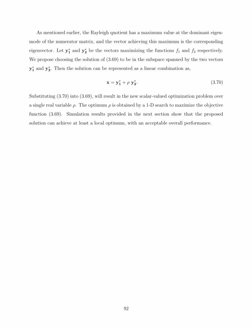
As mentioned earlier, the Rayleigh quotient has a maximum value at the dominant eigen-
mode of the numerator matrix, and the vector achieving this maximum is the corresponding
eigenvector. Let y∗1 and y∗
2 be the vectors maximizing the functions f1 and f2 respectively.
We propose choosing the solution of (3.69) to be in the subspace spanned by the two vectors
y∗1 and y∗
2. Then the solution can be represented as a linear combination as,
x = y∗1 + ρ y∗
2. (3.70)
Substituting (3.70) into (3.69), will result in the new scalar-valued optimization problem over
a single real variable ρ. The optimum ρ is obtained by a 1-D search to maximize the objective
function (3.69). Simulation results provided in the next section show that the proposed
solution can achieve at least a local optimum, with an acceptable overall performance.
92

3.10 Numerical Results
In this section, we present the performance of the proposed energy-efficient power allocation
algorithm, and compare it to “Equal Power Allocation”. It is to be noted that in the equal
power allocation all relays use the same transmission power PR = minPmax, Imax/∑K
i=1 |fRi,P |2.
The noise variance at all nodes, σ2, is set to 1.
In Fig. 3.14, we show the energy efficiency of three power allocation schemes: the proposed
algorithm maximizing the energy efficiency, the power allocation in [115] which maximizes
the SNR, and the equal power allocation. The simulation results are obtained using 106
transmissions. It is shown that, for a 2-relay network, the energy efficiency is almost the
same for the three power allocation schemes. However, for larger networks, the gain starts
to increase. For small to moderate secondary source transmission power PS, the proposed
power allocation offers higher efficiency compared to the SNR-maximizing allocation. The
performance gap increases as the network size increases which is justified by the increased
degrees of freedom in the system. However, for high secondary source power, both schemes
show almost the same performance, and the efficiency starts to decrease. This is due to the
dominance of PS in the denominator of (3.62) for high secondary source powers.
The corresponding outage probability of the secondary system is given in Fig. 3.15, for
interference threshold set to 10 dB, and the individual relays’ power Pmax is set to 0 dB.
The SNR threshold is −3 dB. The results in Fig. 3.15 suggest that for small-size networks,
the energy efficient power allocation has almost no effect on the outage probability. As the
network size increases a slight performance loss is presented by the energy efficient algo-
rithm, compared to the SNR-maximizing allocation. For example, for an 8-relay network,
only 0.1 dB loss occurs in the PS at 10−3 probability of outage. The effect of the inter-
ference threshold Imax on the energy efficiency and the corresponding outage probability
is shown in Figs. 3.16,3.17, respectively. The results are obtained at the secondary source
transmission power PS = 3 dB, and the individual relays’ power Pmax is also set to 3 dB. It
is shown that for small interference threshold values, the proposed algorithm and the SNR-
maximizing algorithm have the same efficiency as satisfying Imax is the limiting constraint in
both problems. However, if this constraint is relaxed by increasing Imax, the proposed algo-
93

−5 0 5 100
0.2
0.4
0.6
0.8
1
1.2
1.4
1.6
1.8
2
Secondary Source Power, PS (dB)
Ener
gy E
fficien
cy
Proposed Energy−Efficient Power AllocaionSNR−Maximizing Power AllocationEqual Power Allocation
K=8
K=6
K=2
K=4
Figure 3.14: The energy efficiency of the secondary network vs the Secondary source trans-
mission power PS for different network size (K). The interference threshold is set to 10 dB
and the individual relays’ Power Pmax is set to 0 dB.
−4 −2 0 2 4 6 810
−4
10−3
10−2
10−1
100
Secondary Source Power, PS (dB)
Outag
e Pro
babil
ity P
out
Proposed Energy−Efficient Power AllocaionSNR−Maximizing Power AllocationEqual Power Allocation
K=2
K=4
K=6
K=8
Figure 3.15: The outage probability of the secondary system Pout vs the secondary source
transmission power PS for different network size (K).The interference threshold is set to 10
dB and the individual relays’ Power Pmax is set to 0 dB. The SNR threshold is −3 dB.
94

rithm achieves higher efficiency. As Imax increases, more tolerance is given in the secondary
network, which allows more power to be used, and hence, the energy efficiency decreases due
to the consumption of more power. Fig.3.17 shows the corresponding outage probability.
Almost no performance degradation between the two power allocation schemes, and both
schemes outperform the equal power allocation.
Next, we show the effect of the individual relay power constraint, Pmax, on the energy
efficiency in Fig. 3.18. The secondary source uses a relatively low transmission power of
PS = 0 dB and the interference constraint Imax is set at 10dB. It is shown that, the energy
efficiency is lower for small values of Pmax. This results from the constraint in (3.64) being the
dominant constraint, and it is satisfied at the upper limit for all relays (i.e. PRi= Pmax∀i).
As Pmax increases, more freedom in the power allocation is obtained, which increases the
SNR, and consequently increases the energy efficiency. However, for a fixed source power
PS, the energy efficiency will eventually saturate at a certain level. The larger the network
size K, the higher is the energy efficiency saturation level. Fig. 3.19 shows the outage
probability of the system (for the same setup of Fig. 3.18) at SNR threshold equals−3 dB. The
outage probability of the three power allocation schemes is the same for small values of Pmax.
Increasing Pmax results in almost no performance degradation between the proposed power
allocation scheme and the SNR-maximizing power allocation, and both schemes outperform
the equal power allocation.
95

−2 0 2 4 6 8 10 12 14 16 18 200
0.2
0.4
0.6
0.8
1
1.2
1.4
1.6
1.8
Interference Threshould, Imax
(dB)
Ener
gy E
fficien
cy
Proposed Energy−Efficient Power AllocaionSNR−Maximizing Power AllocationEqual Power Allocation
K=2
K=8
K=8
K=6
K=4
K=4
K=6
Figure 3.16: The energy efficiency of the secondary network vs the interference threshold
Imax for different network size (K). The secondary source transmission power PS is set to 3
dB and the individual relays’ Power Pmax is set to 3 dB.
−2 0 2 4 6 8 10 12 14 16 18 20
10−4
10−3
10−2
10−1
100
Interference Threshould, Imax
(dB)
Outag
e Pro
babil
ity P
out
Proposed Energy−Efficient Power AllocaionSNR−Maximizing Power AllocationEqual Power Allocation
K=2
K=4
K=6
K=8
Figure 3.17: The outage probability of the secondary system Pout vs the interference threshold
Imax for different network size (K). The secondary source transmission power PS is set to 3
dB and the individual relays’ Power Pmax is set to 3 dB. The SNR threshold is −3 dB.
96

−6 −4 −2 0 2 4 6 80
0.5
1
1.5
2
Individual Relay Power Constraint, Pmax
(dB)
Ener
gy E
fficien
cy
Proposed Energy−Efficient Power AllocaionSNR−Maximizing Power AllocationEqual Power Allocation
K=6K=8
K=4
K=8
K=2
K=6
Figure 3.18: The energy efficiency of the secondary network vs the individual relay power
constraint Pmax for different network size (K). The secondary source transmission power PS
is set to 0 dB. The interference threshold Imax is set to 10 dB.
−6 −4 −2 0 2 4 6 810
−6
10−5
10−4
10−3
10−2
10−1
100
Individual Relay Power Constraint, Pmax
(dB)
Outag
e Pro
babil
ity P
out
Proposed Energy−Efficient Power AllocaionSNR−Maximizing Power AllocationEqual Power Allocation
K=2
K=4
K=8
K=6
Figure 3.19: The outage probability of the secondary system Pout vs the individual relay
power constraint Pmax for different network size (K). The secondary source transmission
power PS is set to 0 dB. The interference threshold Imax is set to 10 dB, and the SNR
threshold is −3 dB.
97

3.11 Summary
In this chapter, we addressed the power allocation problem for underlay non-orthogonal
cognitive relay networks. A QCQP formulation for the average secondary rate optimization
under short-term interference constraint was developed. We obtained the optimal power
allocation and the maximum SNR was derived as the maximum eigenvalue of a channel
dependant matrix. We also proposed an algorithm to solve the power allocation problem
while each secondary node has a limit on its maximum transmission power. Simulation
results show that the obtained power allocation offers significant throughput improvement
over the existing solutions in the literature for similar problems. Finally, an energy efficiency
design for an underlay cognitive network is addressed. A problem for maximizing the power-
normalized SNR of the network using the power allocation of multiple non-orthogonal relays
is formulated. The problem is shown to be a non-convex product of fractional quadratic
functions. Despite the complexity of the problem, we proposed an algorithm to solve the
problem using 1-D search. The obtained power allocation is shown to be energy-efficient
compared to the SNR-maximizing power allocation, with a slight performance loss in the
outage probability.
98

Chapter 4
Antenna Selection for Dual-hop Cognitive Re-
lay Networks
4.1 Introduction
Multiple antenna systems are known for their enhanced reliability and spectral efficiency
[117, 118]. The use of multiple antennas at the cognitive transmitters and/or receivers will
help further enhance their performance (along with cooperation). For example, [119] pro-
posed a precoder for non-regenerative MIMO cognitive relay networks to maximize the sec-
ondary network capacity. In [120], it is shown that with relay selection and clustering, a
MIMO cognitive network with multiple relays can achieve the same growth rate of conven-
tional network (with the absence of the primary system constrains). Using a maximum-ratio
combining (MRC) at the receiver, [121] studied the effect of the maximum interference power
and the maximum transmit power on the secondary system capacity, while [122] studied the
capacity loss due to channel estimation errors.
While MRC achieves the maximum performance in terms of diversity and processing
gains, it suffers from the highest complexity. Alternatively, subset selection of the receiver
antennas offers a diversity gain but sacrifices the processing gain. In fact, the advantages of
subset selection is recognized and implemented in real systems such as IEEE 802.11n and
LTE-A. In general, generalized selection combining (GSC) (which is a subset selection form)
offers a performance/implementation trade-off [123,124]. In [125], diversity gain of transmit
antenna selection with generalized selection combining is quantified. To further reduce the
implementation cost and complexity, GSC shall reduce to the selection of only one antenna,
99

Primary
Transmitter
Primary
Receiver
Primary activity
Secondary activity
Interference Links
R
R
1
Relays
Secondary
Source
Secondary
Destination
2
RK
S
Figure 4.1: Underlay cognitive relay network with secondary receiver equipped with ND
antennas.
namely the selection combining (SC).
In this chapter, we study the performance of cognitive relay networks while the secondary
destination has multiple antennas. we aim at reducing the implementation complexity of the
cognitive destination by only using one radio frequency (RF) chain despite the existence of
multiple receiving antennas. To capture the lost diversity gain, we make use of the availability
of multiple cognitive nodes and allow concurrent relays’ transmission.
4.2 System Model
We consider an underlay secondary network with one source S and one destination D and
K ≥ 2 relays denoted R1, R2, ..., RK . The source S and all relays are assumed to have single
antenna, however, the destination D is equipped with ND antennas. The co-located primary
system consists of a single transmitter-receiver link. The interference on the primary receiver
generated during secondary transmissions must be kept below a pre-defined threshold referred
100
to as the interference temperature, denoted by Imax. Assuming the primary transmitter is
far from the secondary relays as well as the destination D, is a typical and valid assumption
for large networks. Hence, the effect of the primary network on the secondary receivers may
be treated as Gaussian noise or even neglected [59]. Modeling the primary interference as a
Gaussian noise is commonly used in literature as in [65, 125, 126] which is justified through
the central limit theorem (CLT). In the case of single primary interferer, the structure of the
primary signal will have a major role in modelling it into the received secondary SNR. On the
other hand, with multiple primary interferers involved, the statistics of either the maximum
or the summation can be approximated using the central limit theory leading to a Gaussian
approximation.
We also assume block-fading, and all channel coefficients are assumed to be independent.
We assume that a direct link between S and D is absent, and the transmission from S to D
occurs exclusively through the AF relays using a dual-hop protocol. In the first time slot,
S selects the proper transmission power PS to transmit a data symbol to all relays. The
received signal at the ith relay, (i ∈ 1, 2..., K), is given by
yRi=√PS hS,Ri
xS + wRi, (4.1)
where xS is the transmitted data symbol (with E[|xS|2] = 1, where E[·] denote expectation),
and hS,Riis the channel coefficient from S to the ith relay, i ∈ 1, 2..., K, modeled as zero
mean and unit variance circularly symmetric complex Gaussian random variables (CSCGRV),
denoted by CN (0, 1). Here wRiis a complex random variable capturing the effect of the
thermal noise and the interference due to the primary user activities, and is modeled as
CSCGRV with zero mean and variance σ2, denoted by CN (0, σ2). Then, each relay amplifies
its received signal by a variable gain given by,
GRi=
√PRi
eψRi√PS |hS,Ri
|2 + σ2(4.2)
where PRiand ψRi
are the transmission power and the phase correction at the ith relay and
to be designed in the following section. In the second time slot, each relay forwards the
amplified signal to D. To improve the spectral efficiency of the secondary network, all relays
are allowed to transmit simultaneously over the available frequency band (non-orthogonal)
101

following the same model as in Chapter 3. Hence, the received signal vector at D is given by
yD =√PSHR,DGRhS,RxS +HR,DGRwR +wD, (4.3)
whereHR,D ∈ CND×K is the channel coefficient matrix with entries hRi,Djbeing the coefficient
from the ith relay to the jth antenna ofD, modeled as zero mean and unit variance CSCGRV,
denoted by CN (0, 1). GR ∈ CK×K is the beamforming matrix which is a diagonal matrix
with GRi for (i ∈ 1, 2..., K) as the main diagonal elements, and hS,R ∈ CK×1 has hS,Ri
as entries. Here wR ∈ CK×1,wD ∈ CND×1 represent the random variables capturing the noise
and the primary interference effect at the relays and the destination antennas with entries
wRiand wDj
respectively, both modeled as CSCGRV CN (0, σ2).
The overall secondary system can be regarded as a single-input multiple-output (SIMO)
system by rewriting (3.3) as,
yD =√PShxS +w, (4.4)
where h = HR,DGRhS,R and w = HR,DGRwR +wD both ∈ CND×1. However, in order to
reduce the complexity of the secondary destination node, only one RF chain is used with
antenna selection.
The secondary interference to the primary receiver caused by S while transmitting in the
first time slot has a value of IS = PS |gS,P |2 where gS,P is the channel coefficient from S to the
primary receiver. In the second time slot, with all relays transmitting, the total interference
generated at the primary receiver is given by IR =∑K
i=1 PRi|fRi,P |2, where fRi,P is the
channel coefficient from the ith relay to the primary receiver. To ensure proper operation of
the primary user, both IS and IR should be kept below the interference temperature Imax. It is
worth mentioning that, the transmission power of the source PS is determined independently
from the relays power with the only limitation being to satisfy the interference temperature
constraint Imax. Different designs for PS can be adopted such as an adaptive allocation in
the form of PS = Imax/|gs,p|2, or fixed allocation such as Imax/E[|gs,p|2].
4.2.1 Receive Antenna Selection
To overcome complexity and cost limitations due to increased number of radio frequency
chains at the secondary destination node, and yet still gain from the existence of multiple
102

antennas, only one RF chain is used with antenna selection. Using channel estimation, the
receiver evaluates the received SNR from each antenna γ(j)e2e, and then selects the antenna
that achieves the highest SNR, denoted by γ∗. The index of the selected antenna is obtained
by,
j∗ = argmax1≤j≤ND
γ(j)e2e
. (4.5)
How to calculate the values of γ(j)e2e mainly depends on the choice of the power allocation and
phase correction at the relays. In the following section, we present the optimal design of the
beamformer that maximizes the received SNR at a specific antenna.
4.2.2 Optimal Beamforming Design
If the jth antenna at D is selected, the optimal power allocation and the phase corrections
applied at the relays can be used to form a directed beam towards the selected antenna. This
can be accomplished by first using the optimal phase compensation given by,
Ψ(j)R = [ψRi
] = − arghS,R − arg[HR,D]Tj , (4.6)
where arg. is the phase of the enclosed vector, .T is the transpose, and [HR,D]j is the
jth row of the matrix HR,D. Hence, using (3.2),(3.3), and (4.6), the received signal at the
jth antenna can be expressed as,
yDj=
K∑i=1
(√PRi
|hRi,DjhS,Ri
|√PS√
PS |hS,Ri|2 + σ2
)xS +
K∑i=1
(√PRi
|hRi,Dj| wRi√
PS |hS,Ri|2 + σ2
)+ wDj
. (4.7)
Hence, one can obtain an expression for the SNR γ(j)e2e as,
γ(j)e2e = PS ×
(K∑i=1
|hRi,Dj| |hS,Ri
|√PRi√
PS |hS,Ri|2 + σ2
)2
K∑i=1
( √PRi
|hRi,Dj| σ√
PS |hS,Ri|2 + σ2
)2
+ σ2
. (4.8)
Now, the optimal power allocation at the relays that maximizes the received SNR and still
satisfies the interference constraint of the primary network is identical to the optimization
problem given in chapter 3. The optimization problem is given by:
103

P(j)R = argmax
PR
γ(j)e2e,
subject toK∑i=1
|fRi,P |2 PRi≤ Imax. (4.9)
The optimal solution of (4.9) is shown in chapter 3 as:
P(j)R = [P
(j)Ri
] = µj diag
(D− 1
2
)Tv vTD− 1
2
, (4.10)
where diag· is a vector whose elements are the diagonal elements of the enclosed matrix.
Here µj is a positive scaling factor used to satisfy the interference constraint xToptCxopt = Imax,
and is given by µj =Imax
vTD− 12C(D− 1
2
)Tv.
Expanding the matrices with the definitions of their elements, the power allocation at
each relay Ri to form a beam towards antenna j is expressed as:
P(j)Ri
=µj |hRi,Dj
|2|hS,Ri|2(PS |hS,Ri
|2+σ2)[(PS |hS,Ri
|2+σ2)|fRi,P|2+Imax|hRi,Dj
|2]2 .
(4.11)
It can be seen from (4.11) that, aside from the constant µj, the power allocation P(j)Ri
can be
calculated distributively using local channel-state-information (CSI) at each relay. CSI can
be obtained by employing channel estimation techniques using a properly designed signal
known at both the transmitter and the receiver. A feedback control channel is used to
transmit channel estimates to some nodes to use it, or can be shared on a common control
channels.
Now, when the optimal power allocation deployed at the cognitive relays, the correspond-
ing received SNR is maximized to be, γ∗(j)e2e = λmax, where λmax is the dominant eigenvalue
of the channel matrix M. The maximum received SNR is expressed as,
γ∗(j)e2e =
K∑i=1
γ(j)Ri, (4.12)
where,
γ(j)Ri
=|hS,Ri
|2|hRi,Dj|2
|hRi,Dj|2+γsθ|fRi,P
|2|hS,Ri|2+θ|fRi,P
|2 ,
(4.13)
104
with θ = σ2
Imax. It is to be noted that (4.12) suggests a feasible implementation of the antenna
selection algorithm of the previous section. The steps of the antenna selection and power
allocation algorithm are summarized in Algorithm 1.
Algorithm 1 Antenna Selection and Power Allocation Algorithm
Assume Global CSI at D, and Local CSI at Ri ∀ i ∈ 1, 2.., K
D calculates γ(j)e2e from (4.12) ∀ j ∈ 1, 2.., ND
D uses (4.5) to get the index of the selected antenna j∗
D calculates µj∗
D broadcasts j∗ and µj∗ on the control channel
Ri calculates P(j∗)Ri
in (4.11) using local CSI and µj∗
4.3 Clustering
Along with antenna selection, the system complexity can be reduced by allowing only a subset
of the relays to transmit. This is done by dividing the total number of the available relays
into small groups referred to as Clusters. With only one cluster allowed to communicate
with one antenna at the receiver, the complexity of the optimal power calculation and the
feedback time are significantly reduced. In what follows, we introduce two clustering schemes
and study their performance with the receive antenna selection.
4.3.1 Random Clustering
In this scheme, the total number of relays is uniformly divided over equal-size clusters with
the number of clusters equal the number of receive antennas ND. The indices of the relays
Ri are assigned to cluster Cj, j ∈ 1, 2..ND according to the following rule1:
Cj =i :
(j − 1)K
ND
+ 1 ≤ i ≤ j K
ND
. (4.14)
Since the relay-cluster association does not change from transmission to another, it can be
done once at the setup phase of the communication between D and the relays.
1It is assumed that, the number of relays K is an integer multiple of the number of the antennas ND,
resulting in the size of the cluster to be an integer.
105

4.3.2 Max-SNR Clustering
In this scheme, each relay is assigned to the cluster if it maximizes the total received SNR
from its corresponding antenna. It should be noted that, the optimal power allocation in
(4.10) decouples the received SNR into the summation of the individual SNRs generated
by each relay independently. Thus, we propose the Max-SNR clustering scheme where the
indices of the relays Ri are assigned to cluster Cj, j ∈ 1, 2..ND according to the following
rule:
Cj =i : γ
(j)Ri
≥ γ(q)Ri, 1 ≤ q ≤ ND
. (4.15)
A distributed implementation of this scheme is achievable using the following algorithm:
Algorithm 2 Max-SNR Relay-Cluster Association Algorithm
Assume Local CSI at Ri ∀ i ∈ 1, 2.., K
Ri calculates γ(j)Ri
from (4.13) ∀ j ∈ 1, 2.., ND
Ri solves j∗ = argmax1≤j≤ND
γ(j)Ri
Ri associates itself with cluster C∗
j
4.4 Performance Analysis
In what follows we analyze the performance of the proposed relay clustering schemes in-terms
of the system outage probability.
4.4.1 Random clustering case:
In this section, we derive the statistics of γ∗ which will be used to assess the performance
of the secondary system. Given the selection rule in (4.5), the output SNR of the selected
antenna is given by
γ∗ = max1≤j≤ND
γ(j)e2e,Random
, (4.16)
106
where γ(j)e2e,Random is the end-to-end SNR resulting at the jth antenna through its connecting
cluster using random clustering, and is given by,
γ(j)e2e,Random =
∑Cj
γ(j)Ri. (4.17)
It should be noted that, for random clustering all the clusters have equal and fixed sizes |Cj|,
with |Cj| = AC = KND
∀j.
The outage probability of the cognitive network with random clustering, PRout, defined as
the probability of the end-to-end SNR of the selected antenna (or cluster) drops below a
certain threshold γth. PRout is obtained in a closed-form as,
PRout(γth) =
γACNDth e
−NDγthµγ
[(AC − 1)!]NDµACNDγ
ND∑k=0
αkγkth. (4.18)
4.4.2 Max-SNR clustering case:
In this section we study the outage probability of the Max-SNR clustering scheme. First, we
start by analysing the relay-cluster association scheme. It is shown in (4.15) that a relay is
associated to a cluster j if the SNR of the corresponding antenna is the maximum. Therefore,
the contribution of relay Ri to the total received SNR from its cluster Cj is given by,
γ(j∗)Ri
= max1≤j≤ND
γ(j)Ri
. (4.19)
Hence, the total SNR received from the cluster Cj, is given by
γ(j)e2e,Max =
∑Cj
γ(j∗)Ri
(4.20)
where the size of the cluster Cj is Aj.
The outage of the cognitive network occurs when all the clusters/antennas experience
outage. This is expressed as follows,
Pout(γth) = ΠNDj=1Pout,j(γth|Aj), (4.21)
where Pout,j(γth|Aj) is the outage probability of cluster Cj of size Aj, obtained as follows.
Form the description of the clustering scheme and the definition of γ(j∗)Ri
in (4.19), the CDF
107

of γ(j∗)Ri
, is given by;
Fγ(j∗)Ri
(x) =
[Fγ(j)Ri
(x)
]ND
(4.22)
where Fγ(j)Ri
(x) is the CDF of γ(j)Ri. Given that, γ
(j)Ri
is tightly approximated as an exponential
random variable with mean µγ given in (3.34), we can rewrite Fγ(j∗)Ri
(x) as,
Fγ(j∗)Ri
(x) =
ND∑n=0
(ND
n
)(−1)ne
− nxµγ . (4.23)
Now, the total SNR received from the cluster Cj, is given by γ(j)e2e,Max =
∑Cjγ(j∗)Ri
. The outage
probability of the cluster Cj is, then, given by
Pout,j(γth) = Pr(γ(j)e2e,Max ≤ γth)
= Pr(∑Cj
γ(j∗)Ri
≤ γth)
≤ Pr( min1,2...Aj
γ(j∗)Ri
≤ γthAj
) (4.24)
where the last line in (4.24) made use of the approximation∑
Cjγ(j∗)Ri
≤ Aj min1,2...Ajγ(j∗)Ri
.
Let Y be the random variable min1,2...Ajγ(j∗)Ri
. The CDF of Y is given by
FY (y) = Pr(Y ≤ y) = 1− ΠAj
i=1Pr(γ(j∗)Ri
≥ y)
= 1−[1− F
γ(j∗)Ri
(y)]Aj
. (4.25)
Now, substituting (4.23) into (4.25) and replacing y = γthAj
, we obtain
Pout,j (γth|Aj) = 1−
[1−
ND∑n=0
(−1)n(ND
n
)e− nγth
Ajµγ
]Aj
. (4.26)
Given the probabilistic nature of the relay-cluster assignment, an averaging of all possible
combination of cluster sizes should be taken into account. This can be complied by noting
that the sizes of clusters are jointly distributed as a multinomial random variable with equal
probabilities pi =1ND
. Hence, the total system outage probability is given by,
Pmaxout (γth) =
∑ΛK=k1,...kND
K!
k1!...kND!ND
KΠNDj=1Pout,j(γth|Aj). (4.27)
108

where ΛK is the set that includes all possible permutations of the ND numbers k1, k2...kND
that add up to K (i.e∑ND
i=1 ki = K). For instance, if K = 3 and ND = 2, then ΛK =
(0, 3), (3, 0), (2, 1), (1, 2). It should be noted that Pout(γth|0) = 1 is the outage probability of
an empty cluster.
4.5 Simulation Results
In this section, we present the performance results of the proposed antenna selection scheme
and the power allocation at the secondary network through the derived expressions and
simulation.
4.5.1 Antenna Selection Only
First, we present the performance of antenna selection at the secondary destination for dif-
ferent network sizes. The outage probability is defined as Pout(γth) = Pr(γ(j∗)e2e ≤ γth), where
γ(j∗)e2e is the SNR of the selected antenna. Fig. 4.2 shows the outage probability Pout versus
γs (the secondary source power PS measured relative to the noise power σ2) for a target
SNR γth = 3 dB. The interference temperature Imax is set at 7 dB and the noise power is
normalized to 1. It is noted that, increasing the number of antennas ND for a fixed relaying
network size K enhances the outage performance by increasing the diversity order. However,
increasing K from 2 to 3 for a fixed ND achieves 3 dB SNR gain, while doubling ND from
2 to 4 only achieves 1.5 dB for a 2-relay network. This leads us to the non-intuitive result,
that the network size K has an impact on the outage probability higher than the impact of
the number of receive antennas ND. We also compare the performance of the secondary sys-
tem with multiple relays and antenna selection to the opportunistic relay selection. In such
scheme, a single relay with best SNR is selected and the received signals from all antennas
are combined. It can be seen form Fig 4.2 that the system with multiple active relays and
antenna selection outperforms opportunistic relay selection while using multiple antennas for
reception.
109

−4 −2 0 2 4 6 8 10 12 14 16 1810
−4
10−3
10−2
10−1
100
γS (dB)
Out
age
Prob
abilit
y P ou
t
ND
=2
ND
=4
ND
=6
K=2
K=2
K=3
K=3
Figure 4.2: Outage probability of antenna selection for different values of ND, for number of
relays K = 2 and 3. The interference temperature Imax=7 dB and the target SNR γth = 3
dB. Solid: Multiple Relays, Dotted: Opportunistic Relay Selection.
4.5.2 Effect of Power Allocation Scheme
Second, we examine the effect of the power allocation at the relays by simulating the outage
probability Pout of the cognitive network employing the optimal power allocation in (4.10)
compared to the equal power allocation where PRi= Imax∑K
1 |fRi,P|2 . We also include the perfor-
mance of opportunistic relays selection with the power of the selected relay PRi∗ = Imax
|fRi∗ ,P |2 .
While optimal power allocation in (4.10) allows the distribution of the power among the relays
such that the interference constraint of the primary user is satisfied, it utilizes the dominant
eigenmode of the channel matrix which minimizes the self interference among the relaying
channels and transforms them into orthogonal channels. On the other hand, the equal power
allocation only satisfies the primary user interference constraint by sharing it equally among
the relays. Fig. 4.3 clearly shows that the optimal power allocation outperforms the equal
power allocation.
110

4.5.3 Relay Clustering and Antenna Selection
Up to this end, all relays are allowed to communicate with all the available antennas at
the destination. Next, we present the performance of the clustering techniques, where only
a subset of the relays is allowed to communicate with only one antenna. We compare the
performance of the proposed clustering schemes, namely, the Random clustering and the
Max-SNR clustering in Fig. 4.4. Here, we study the system with K = 6 relays for all cases.
For Random clustering, the size the cluster is fixed and increasing ND will directly result in
decreasing the number of relays per cluster which leads to a performance degradation. This
observation agrees with the conclusion form Fig.4.2 and further elaborated in Fig 4.5 and
4.6. However, for the Max-SNR clustering, the cluster size is a random variable (binomial
with parameters K and 1ND
), which suggests that there exist a non-zero probability that the
selected cluster/antenna will have a size higher than the random clustering case. Hence, a
superior performance for the Max-SNR clustering scheme is achieved. We also included the
case of a single-antenna (no clustering/no-antenna selection) and K = 6 as a bench mark as
−4 −2 0 2 4 6 8 10 12 14 16 1810
−4
10−3
10−2
10−1
100
γs (dB)
Outa
ge P
roba
bility
Pou
t
Optimal Power Alloaction, ND
=4
Equal Power Alloaction, ND
=4
Opportunistic Relay Selection, ND
=4
Optimal Power Alloaction, ND
=2
Equal Power Alloaction, ND
=2
Opportunistic Relay Selection, ND
=2
Figure 4.3: Outage probability of antenna selection for different power allocation schemes,
with the number of relays K = 3, Imax=7 dB.
111

−4 −2 0 2 4 6 8 10 12
10−4
10−3
10−2
10−1
100
γS (dB)
Out
age
Prob
abilit
y P ou
t
Random Clustering, ND
=2
Max SNR Clustering, ND
=2
Random Clustering, ND
=3
Max SNR Clustering, ND
=3
No Clustering, ND
=1
Simulation
Figure 4.4: Outage probability of antenna selection and relay clustering, for different values
of ND, with number of relays K = 6, Imax=7 dB using optimal power allocation.
it has the same degrees of freedom. As shown the performance of Max SNR clustering with
antenna selection is comparable to the single-antenna case for low γs. As γs increases, the
Max-SNR selection shows a better performance than the single-antenna case.
Fig. 4.5 plots the outage probability versus the number of relays K for the two proposed
clustering schemes with antenna selection where the secondary destination has ND = 2
antennas. It is shown that, increasing the number of relays (while fixing the number of
antennas), results in increasing the number of relays per cluster (in case of random clustering)
which enhances the performance. Also, the average cluster size increases for the case of Max
SNR clustering which shows a superior performance compared to the random clustering.
112

2 4 6 8 10 12 14 16 18 2010
−4
10−3
10−2
10−1
100
Number of Relays K
Outa
ge P
roba
bility
Pou
t
Random Clustering, γth
= 3 dB
Max SNR Clustering, γth
= 3 dB
Opportunistic Relay Selction, γth
= 3 dB
Random Clustering, γth
= 5 dB
Max SNR Clustering, γth
= 5 dB
Opportunistic Relay Selction, γth
= 5 dB
Simulation
Figure 4.5: Outage probability of antenna selection and relay clustering vs the number of
relays K while ND is fixed (ND = 2), Imax=7 dB using optimal power allocation for both
random clustering and Max SNR clustering.
Fig. 4.6 completes the picture by plotting the outage probability as the number of anten-
nas increases for a fixed number of relays. A reverse behaviour is encountered as the number
of relays per cluster decreases. It is shown that, as the number of antennas increases for a
fixed number of relays, the cluster size decreases, and hence the outage probability increases.
It is also shown that, both clustering schemes outperform opportunistic relay selection. We
also compare the simulation results of the two clustering schemes to the analytical expressions
of the outage probability in Fig. 4.7 for random clustering, and in Fig. 4.8 for Max-SNR
clustering where both figures show a perfect match.
113

2 4 6 8 10 12 14 16 18 20
10−4
10−3
10−2
10−1
100
Number of Antennas ND
Out
age
Pro
babi
lity
Pou
t
Random Clustering, γth
= 3 dB
Max SNR Clustering, γth
= 3 dB
Opportunistic Relay Selection, , γth
= 3 dB
Random Clustering,γth
= 5 dB
Max SNR Clustering, γth
= 5 dB
Opportunistic Relay Selection, , γth
= 5 dB
Simulation
Figure 4.6: Outage probability of antenna selection and relay clustering vs the number of
antennas ND with K = 20 relays, Imax=3 dB using optimal power allocation.
−5 −4 −3 −2 −1 0 1 2 3 4 5 610
−4
10−3
10−2
10−1
100
γs (dB)
Ou
tag
e P
rob
ab
ility
Po
ut
Analytical
Simulation
ND
=4ND
=3ND
=2
Figure 4.7: Analytical and simulation results of outage probability for K = 12 and different
ND setups, Imax=5 dB using optimal power allocation for random clustering.
114
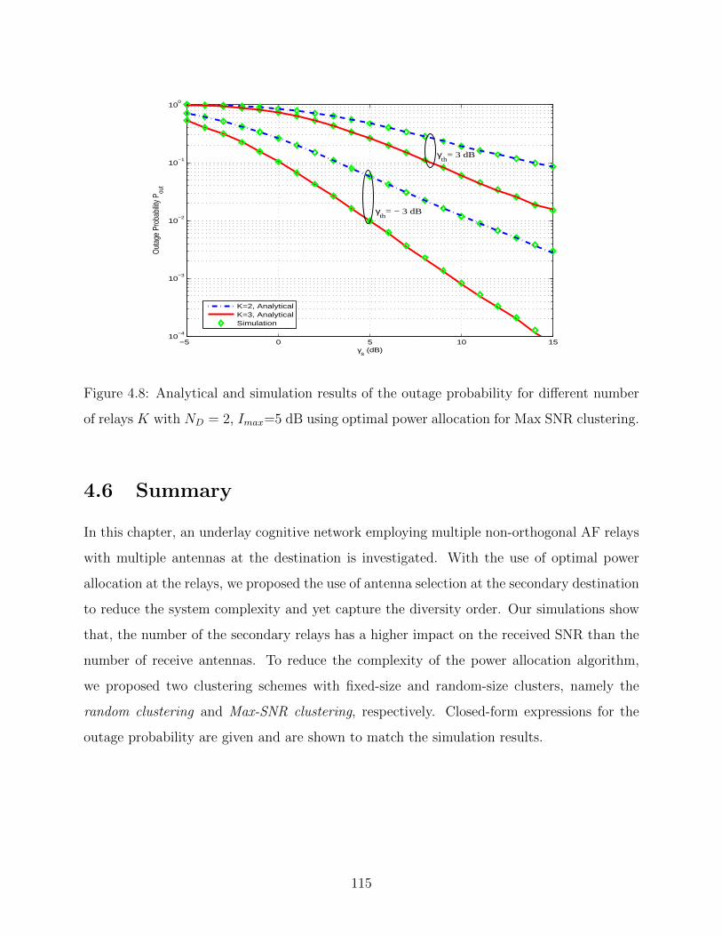
−5 0 5 10 1510
−4
10−3
10−2
10−1
100
γs (dB)
Out
age
Prob
abilit
y P ou
t
K=2, AnalyticalK=3, AnalyticalSimulation
γth
= 3 dB
γth
= − 3 dB
Figure 4.8: Analytical and simulation results of the outage probability for different number
of relays K with ND = 2, Imax=5 dB using optimal power allocation for Max SNR clustering.
4.6 Summary
In this chapter, an underlay cognitive network employing multiple non-orthogonal AF relays
with multiple antennas at the destination is investigated. With the use of optimal power
allocation at the relays, we proposed the use of antenna selection at the secondary destination
to reduce the system complexity and yet capture the diversity order. Our simulations show
that, the number of the secondary relays has a higher impact on the received SNR than the
number of receive antennas. To reduce the complexity of the power allocation algorithm,
we proposed two clustering schemes with fixed-size and random-size clusters, namely the
random clustering and Max-SNR clustering, respectively. Closed-form expressions for the
outage probability are given and are shown to match the simulation results.
115

Chapter 5
Channel Estimation for LTE-MTC Systems
5.1 Introduction
In the previous chapters, we studied the cognitive relay networks as a strong candidate to
enable the IoT framework. However, some of the IoT applications might require transmission
priority, wider coverage, or high data rates. In such cases, cellular networks offer a good
solution with their large coverage and flexible data rates. Scenarios defined by the 3rd
Generation Partnership Project (3GPP) standardization body emerge as the most promising
solutions to enable cellular infrastructure of M2M communications. LTE CAT-M is a special
category of user equipments supporting MTC features, has been incorporated by the 3GPP
to Long-Term-Evolution (LTE) specifications.
In conventional LTE systems, the network provides the UE with Downlink Control Infor-
mation (DCI) messages sent over the Physical Downlink Control Channel (PDCCH) [127].
An Enhanced PDCCH (EPDCCH) is introduced in LTE-A Release-11 to achieve better spec-
tral efficiency by exploiting frequency selectivity and beamforming and also to provide greater
flexibility of dynamic allocation of control channel resources. The DCI messages dynamically
provide both downlink and uplink scheduling and detection information on how to receive the
data (e.g. modulation, coding, resource assignment, and power control). Thus, the downlink
control channel is one of the most important channels and represent the precondition for the
correct data decoding. Since LTE-MTC has different challenges and objectives, conventional
control channels have to be revised [128]. To cope with the new challenges of MTC, new
specifications for the control channel for MTC is defined as MTC-PDCCH or MPDCCH.
Coherent detection of the MPDCCH is a must and requires channel knowledge, hence,
116

special Demodulation Reference Signals (DMRS) are attached to MPDCCH to allow pilot-
aided channel estimation. However, the use of conventional channel estimators with the new
MPDCCH will not be efficient in terms of complexity and performance. In fact, channel
estimation is identified as one of the main areas that should be further improved for CAT-M
UEs [129].
In this chapter, we propose a channel estimation algorithm for the newly introduced
MPDCCH in the specifications of the LTE-A CAT-M. The proposed technique aims at re-
ducing the complexity of the channel estimation of the MPDCCH as minimum as possible.
In order to achieve this goal, we propose using the simple Least Squares (LS) estimation to
estimate the pilots signals, followed by two stage first-order polynomial interpolation (linear)
to obtain the channel estimates at every point in the time-frequency grid. We also address
the use of the repeated transmissions to enhance the performance of the proposed technique.
5.2 MTC Physical Downlink Control Channel
To improve the spectral efficiency of the control channel, the EPDCCH was introduced to
the LTE-A Release-11 standard as an alternative to the legacy PDCCH which is mapped to
the full occupied bandwidth. For MTC applications, decoding PDCCH is not possible since
the UE is limited to only 1.4MHz. Furthermore, coverage enhancement can be achieved
by employing EPDCCH that supports beamforming which increases coverage by directing
the base station’s power towards the UE. In addition, the EPDCCH can be repeated to
achieve SNR gain in the lack of spatial diversity and frequency diversity. For these reasons,
EPDCCH has been chosen to be the starting point towards designing the new MTC control
channel MPDCCH. However, special requirements have been adapted to best suite the new
MTC platform and to support the required coverage with reasonable complexity and power
consumption. The new set of features for MPDCCH require defining new set of downlink
control formates [130], and adding a possibility for a common UE to access the control
channel. In addition, repetition and frequency hopping are introduced to enhance the control
channel assignment procedure.
117

NB2
NB15
NB0
1 PRB
20
MH
z
99
Legacy control
symbols
MP
DC
CH
(4 P
RB
set
)
MPDCCH
(2 PRB set)
MPDCCH
(2 PRB set)
MPDCCH
(4 PRB set)
1 sub-frame (1ms)
14 OFDM symbols
1 PRB
12
su
bca
rrie
rs
Slot 0 Slot 1
0.5 ms0.5 ms
0
DMRS REs for
P107 and P108
Cell specific
RSs
First RE for one
EREG
Legacy
control REs
Time7
2 s
ub
carr
iers
Fre
q.
0
0
0
0
0 0
4
5
6
7
0
1
2
3
8
9
10
11
0
12
13
14
15
0
2+4 PRB
set mode
4 PRB set
mode
2 PRB set
mode
Subcarrier order
for various EREGs
98
97
96
95
94
93
92
19
18
17
16
15
14
7
6
5
4
3
2
1
0DMRS REs for
P109 and P110
Figure 5.1: A single PRB structure for MPDCCH showing locations of DMRS and EREG
start for Normal CP mode.
5.2.1 MTC Control Channel Assignment
5.2.1.1 Control Channel Aggregation and Mapping
Similar to EPDCCH, the MPDCCH can be configured with 1 or 2 physical resource block
(PRB) sets. However, for MTC, both sets will either be localized or distributed. Unlike
EPDCCH, MPDCCH set sizes can be configured only to be either 2 or 4 PRBs. Thus, the
only option to have 6 PRBs allocated to MPDCCH (which is the maximum), is by using 2 sets;
one with 2 PRBs and the other with 4 PRBs. Hence, this assignment is referred as the “2+4”
configuration. Fig. 5.1 shows the possible set assignment for MPDCCH. The MPDCCH is
backward-compatible with the EPDCCH, hence it is frequency-multiplexed with the data
channel PDSCH. The mapping of the MPDCCH to the physical resource elements is also
similar in principle to the conventional EPDCCH [131]. With the conventional EPDCCH,
the REs are grouped together into Enhanced Resource Element Groups (EREGs) (with 9
REs per EREG for Normal CP mode and 8 REs per EREG for Extended CP mode). The
118

EREGs are then grouped into Enhanced Control Channel elements (ECCEs) with 1 ECCE
being formed from 4 EREGs for Normal CP and 8 EREGs for Extended CP type. This gives
36 REs per ECCE for the Normal CP type and 64 REs per ECCE for the Extended CP
type. As shown in Fig. 5.1, a single PRB pair is shown for Normal CP mode. First, notice
the Demodulation Reference Symbols (DMRS) within the PRB pair. These are used as the
coherent reference to demodulate the signal. The remaining REs are numbered from 0 to
15 in a cyclical fashion moving first in frequency and then in time. The REs with the same
number form 1 EREG. It is also worth mentioning that during resource element mapping for
MPDCCH, the REs will be punctured by the cell specific RS as well as by the legacy control
channel REs.
Each MPDCCH is then formed from 1 or more ECCEs being aggregated together. The
aggregation levels have been revised for MPDCCH to be 1, 2, 4, 8, 16, or 24 ECCEs for
Normal CP and 1, 2, 4, 8, and 12 for Extended CP. The aggregation is the mechanism for
rate adaptation to the channel conditions and payload size. The higher the aggregation level,
the lower the coding rate and the lower the SNR at which the signal can be demodulated.
Unlike the PDCCH/EPDCCH for which the maximum aggregation level is 8, the maximum
aggregation level for the MPDCCH is 24 formed by using multiple PRBs. This gives the
lowest coding rate, allowing for better coverage. The aggregation level of 24 is achieved using
2 RB sets, one with 2 PRBs and another one with 4 PRBs.
There are two different mappings of the original EPDCCH in forming ECCEs: localized
and distributed. MPDCCH inherits similar mapping. In localized mapping, all EREGs that
constitute an ECCE are located within the same PRB pair. With the distributed mapping,
the ECCE is formed from EREGs in multiple PRBs that are distributed across the allocated
PRB pairs for the control channel. In fact, the localized mapping allows the system to exploit
frequency selectivity. The distributed mapping gives more diversity for those situations where
frequency selectivity can not be exploited.
A significant difference between EPDCCH and MPDCCH is the time relation between
the control channel and the corresponding shared channel [132]. To relax the latency re-
quirements at the UE side, 3GPP has decided to schedule an MPDCCH in subframe m for
the corresponding shared channel at subframe m+ p where p is a positive integer and p = 0.
119

Table 5.1: Candidate Table for CE Mode A in LTE-MTC
No. of PRBs Possible candidate for blind decoding
2+4
2 PRB set [2,R1,14,R1,1] [4,R2,18,R2,1]
4 PRB set [8,R1,216,R1,1][8,R2,216,R2,1]
[8,R3,116,R3,1]
2+4 PRB set [24,R1,124,R2,124,R3,124,R4,1]
2 [2,R1,24,R1,18,R1,12,R2,2
4,R2,18,R2,12,R3,24,R3,1
8,R3,12,R4,24,R4,18,R4,1]
4 [2,R1,14,R1,18,R1,116,R1,1
2,R2,14,R2,18,R2,116,R2,1
2,R3,14,R3,18,R3,116,R3,1
2,R4,14,R4,18,R4,116,R4,1]
However, a pipeline assignments may occur such that the PDSCH can be received in sub-
frame m + 1 concurrently with a scheduled MPDCCH that configures the detection of the
PDSCH in sub-frame m+ 2, for example.
5.2.1.2 Blind Decoding and Repetition
To blindly decode one candidate in conventional LTE systems, the following is required:
static parameters including the CP type, the mapping type, and the user identity represented
by the Radio Network Temporary Identifier (RNTI) and dynamic parameters including the
candidate index, the DCI size, and the aggregation level. It has been agreed for MTC that
the new DCI formats have the same size to reduce the number of trials for blind decodes.
Also, to enable low cost UE, MPDCCH has been designed to support a maximum of 20 trials
for blind decoding for both common search spaces (CSS) and the user-specific search spaces
120

(USS). In addition to the static parameters, each blind decode candidate in MPDCCH is
then defined by an aggregation level and a number of repetitions. The number of repetitions
define the amount of time diversity and soft combining that can be applied to this candidate.
3GPP specifications defines the number of repetitions by signalling the maximum number
of repetitions, Rmax, to the UE. Each CE level has a different value configured through
the system information. From Rmax, a set of repetition levels are defined including (R1,
R2, R3, and R4). For example, this set in the USS is defined as follows: (1) If Rmax = 1,
then R1 = Rmax. (2) If Rmax = 2, then Rmax = 2R1 = R2. (3) If Rmax = 4, then
Rmax = 4R1 = 2R2 = R3. (4) If Rmax ≥ 8, then Rmax = 8R1 = 4R2 = 2R3 = R4. The set of
blind decodes for mode A are defined by Table 5.1 [133]. The entries in the table enumerate
the blind decodes as: aggregation level, repetition index (R1, R2, R3, and R4), number of
blind decodes.
5.2.1.3 Frequency Hopping
With the small bandwidth offered to MTC UE, there is a significant loss of frequency diversity.
To recover portion of this gain, the MTC LTE system will make use of frequency hopping.
Thus, transmissions will hop from one narrowband to another [134]. Frequency hopping
regains some of the frequency diversity but it introduces new challenges. One issue is that
the UE will need to re-tune every time it hops, and this re-tuning takes time which might
affect the overall throughput. 3GPP working group has decided that 2 OFDM symbols worth
of time is needed for re-tuning. Further, re-turning will take place during the legacy control
channel symbols which will be discarded anyway by the MTC UE. This choice of re-tune time
and period reduces the chance of loosing the a considerable amount of network throughput.
Another issue with frequency hopping is that the UE and eNodeB both need to know the
hopping pattern. This needs to be signalled or must be determinable from certain system
parameters. The new signalling introduces an overhead to the system. The way that the
hopping parameters are signalled depend on the processed channel.
For MPDCCH, the first NB is determined without any new higher layer configuration
involved (i.e. it is specified in the system information messages). The other narrowbands are
determined using a single configurable offset. The offset, signalled in the system information,
121

is cell-specifically configured and applicable to all CE levels. In CE mode A, the hopping is
turned on or off dynamically by higher-layer signalling in the DCI if the hopping is enabled.
The number of NB for hopping is either 2 or 4. This parameter is signalled to the UE and
it is cell-specific.
With frequency hopping, the channel estimation will need to be restarted whenever hop-
ping is scheduled. This will have a negative effect of the accuracy of the channel estimates
if time diversity is used to enhance the performance. Based on the specifications [135], the
MPDCCH transmission will stay on one NB for Y subframes, where Y is in the range of
2-8 subframes to allow some benefit of cross-subframes channel estimation. This value Y is
called the frequency hopping interval and it is cell-specific. There are 4 values signalled to
specify the frequency hopping interval for all channels in a specific channel direction and UE
mode, namely mode A DL, mode B DL, mode A UL, mode B UL. For FDD and mode A,
the values that this parameter may take are among the set 1, 2, 4, 8. For mode B they
take values in the set 2, 4, 8, 16.
5.3 System and Signal Models
Fig. 5.2 shows the downlink transmitter/receiver chain for the MPDCCH. At the transmitter
side, the control information (DCI payload with length K) is first generated. After CRC
attachment which is mainly 16 bits CRC code, the bits are coded with a rate 1/3 tail-
biting convolutional code, interleaved, and then rate matched to fit the amount of resources
used for the control channel transmission. The rate matching output is scrambled by a cell
specific random sequence where the output is QPSK modulated. The resource elements are
mapped, along with the reference symbols, to the proper control channel elements on the
time/frequency grid according to a predefined scheduler for this control segment. According
to LTE-MTC specifications, the control channel candidate will be repeated within a set of
consecutive sub-frames. The time domain OFDM symbols are synthesized by employing an
Inverse Fast Fourier Transform (IFFT). To reduce the effect of Inter-Symbol Interference
(ISI), the last Ng samples of the symbol are copied to the beginning of each OFDM symbol
in order to form the cyclic prefix.
122

FFTChannel
Equalization
Channel
Estimation
CP
removal
Time &
Freq. Sync.
RE
Demapper
Const.
DemapingDeScrambler
DeInterleaverSoft
comb.
Blind Decoding
h(n)
DCI
Gen.
Conv.
Encoder
Inter. & Rate
Maching
QPSK
Mod.
CRC
check
RE
MapperRepetition
CRC
attachIFFT
CP
InsertionScrambler
Rate
Dematching
TailBiting
Conv. Decoder
Control Channel Transmitter
Crystal
ADC
mixer
Figure 5.2: Block diagram for the transmitter/receiver model for the control channel simu-
lation in LTE-MTC system
The eNodeB communicates with UE over the channel h(n). The receiver is subjected
to AWGN, z(n). In the frequency domain, the channel should be estimated and equalized.
As part of the decoding, the CCEs are combined through the resource element demapper to
form the control channel candidate back. The constellation demapper is employed to obtain
the soft bits which are descrambled by the same sequence applied at the transmitter side.
Depuncturing is allowed by the rate dematching to bring the number of soft bits back to
3× (K + 16) which are then deinterleaved. If repetition is involved at the transmitter side,
soft combing is applied across sub-frames to increase the reliability of the soft bits. This
combining is assumed to be MRC mechanism. Once the soft combining is complete, the soft
bits are decoded by a typical tail-biting convolutional decoder and then CRC check is applied
to decide whether the block is correctly received or not.
The complex baseband equivalent channel of the wireless channel impulse response [136]
can be represented as,
h(t, τ) =∑m
νmδ(t− τm) (5.1)
where δ(t) is the conventional impulse function, τm is the mth path delay, and νm is the
corresponding time varying complex amplitude. The frequency domain transfer function
H(l, k) represents the channel gain at each sub-carrier position k in each OFDM symbol l.
For a multiple transmit antenna system, the received signal at the receiver antenna represents
the combined version of the transmitted streams. Let the frequency domain received signal
123

R(l, k) at OFDM symbol l and sub-carrier index k be given by (5.2), where Sj(l, k) is the
transmitted sub-carrier from antenna port j, Hj(l, k) is the channel transfer function from
antenna port j, and Z(l, k) represents the additive white Gaussian noise. All have been
considered at OFDM symbol l and sub-carrier k.
R(l, k) =∑j
Sj(l, k)Hj(l, k) + Z(l, k) (5.2)
5.4 Channel Estimation For MPDCCH
5.4.1 Pilot Structure
Frequency domain multiplexing of the control information with data was adopted to facilitate
frequency selective scheduling of the downlink and uplink assignments and frequency-domain
Inter-Cell Interference Coordination (ICIC). The DMRS are employed by antenna ports 107
to 110, where each port may be taken to indicate one physical antenna, for a total of up to
4 transmitting antennas. For normal CP type, antenna ports 107 and 108 share the same
subcarrier locations for their DMRS. Similarly antenna ports 109 and 110 share the same
subcarrier locations. Note that, the DMRS transmitted by the different antennas that share
the same subcarrier locations are orthogonal. Also, it is worth to mention that an MPDCCH
candidate can be transmitted through a single layer system when localized transmission is
configured. On the other hand, to gain more diversity in distributed transmission mode,
the symbols that belong to the same candidate are mapped onto two sets of orthogonal
subcarriers. These two sets are transmitted by two transmit antennas which involve orthog-
onal precoding. Thus, in all cases, a single subcarrier will be observed according to a single
antenna transmission.
For the transmitted pilot tones at OFDM symbol lp and subcarrier index kp, the trans-
mitted pilot Sj(lp, kp) is represented, by,
Sj(lp, kp) = W j(lp, kp)x(lp, kp), (5.3)
where x(lp, kp) is some pseudo-random unitary signal value (of QPSK nature) transmitted
by all antennas at subcarrier (lp, kp) and Wj(lp, kp) is the value of a binary orthogonal cover
124

code for antenna port j at subcarrier (lp, kp). The cover code is of length 4 and is constructed
based on the two vectors [1 1 1 1] and [1 -1 1 -1], where the first vector is attached to odd
numbered ports and the second vector is assumed for the even ones. The code sequence for
each antenna port is applied in the time dimension either in the forward or reverse order.
This order is reversed in the frequency dimension.
5.4.2 Pilot Signal Estimation
Although the general channel estimation problem in case of single antenna systems is two-
dimensional [95] (i.e., has to be carried jointly in the frequency and time domains), it is
normally separated into two one-dimensional estimation steps to simplify the implemen-
tation [137]. In this context, the channel estimation problem can be considered over one
OFDM symbol (specifically the symbol containing the DMRS) to exploit the frequency do-
main characteristics. Prior to any signal processing for the channel estimation algorithm in
the MPDCCH, the Channel Transfer Function (CTF) is estimated in the frequency domain
at the pilot positions first.
Let (lp, kp), (lp, kp+5), and (lp, kp+10) be the three subcarriers of one resource block that
carry consecutive DMRS in the same OFDM symbol. The channel vector from antenna port j
at the pilot subcarriers can be defined as hjp = [Hj(lp, kp) Hj(lp, kp+5) Hj(lp, kp+10)]T , where
(.)T is for the transpose operator. The corresponding pseudo-random signal can be defined by
the diagonal matrix X = diag[x(lp, kp) x(lp, kp + 5) x(lp, kp + 10)]. If the precoding code for
antenna port j is also represented by the diagonal matrix Wj = diag[W j(lp, kp) Wj(lp, kp +
5) W j(lp, kp+10)], Then, the received subcarriers vector at the pilot positions can be defined
as,
rp = XWjhjp +XWihip + z (5.4)
where z is the noise vector, i ∈ 107, 108 and j ∈ 109, 110 based on the DMRS of
interest. Since Wi is orthogonal to Wj and the channels from various antenna ports are
typically assumed to be uncorrelated, we get the channel estimation at the pilot locations for
antenna port j using the Least Squares (LS) estimation given by,
hjp = (XjHXj)−1(Xj)
Hrp (5.5)
125

where, Xj =[Wj]−1
X, and (.)H is the Hermitian.1
Because the number of pilot sub-carriers is always fewer than the number of information-
carrying sub-carriers, interpolation across time and frequency is required to obtain a channel
estimate at each sub-carrier in the time-frequency grid. 2-D interpolation is required in
order to obtain a channel estimate for each antenna port at each sub-carrier H from hp.
The channel estimate is obtained using, H = Chp, where C is a matrix representing the
filter operation (i.e., the interpolation process) applied to the channel estimates at the pilot
positions. Typically, the implementation of interpolation using 2-D filters increases the com-
plexity of the channel estimation algorithm. However, using the separability property [138],
2-D interpolation can be achieved using two cascaded 1-D filters to implement the time and
frequency interpolations. In this method, H is divided into two sets Ct and Cf , where Ct
is a filter operating along the time direction, while Cf is a filter operating in the frequency
direction.
In order to calculate these filter coefficients, a variety of techniques can be used. In the
following, we will present some of the commonly used techniques and shed some light on
their suitability for MPDCCH.
5.4.2.1 MMSE Interpolation Approach
The optimum MMSE interpolation has been well studied in the literature [139]. In [140],
using two 1-D Wiener filters can achieve performance near to the optimum 2-D nonseparable
Wiener filter but with much reduced complexity. The 1- D Wiener filter for interpolating the
kth sub-carrier channel from its neighboring pilots in the lth OFDM symbol is given by
HMMSEl = (ρp,p + ηI)−1ρHl,p (5.6)
where ρp,p is the autocorrelation matrix of the CFR at the pilot subcarriers, ρl,p is the cross
correlation of CFR between the pilot subcarriers and the one to be estimated, η is a factor
depending on the operating SNR, and I denotes an identity matrix of the right dimension.
1Similarly, the channel estimates at the pilot positions for antenna port i is formulated as Hip =[
Wi]−1
X−1rp. For simplicity, we will drop the superscripts i and j, and the reader can assume identi-
cal processing for both antenna ports.
126

This type of filter can be used across the time and frequency dimensions. However, the MMSE
estimation here requires knowledge about ρp,p , ρl,p and the operating SNR. To obtain such
information, multiple techniques have been proposed to approximate parametric model for
the CFR autocorrelation function in the frequency dimension [141]. The model involves the
use of two parameters to approximate the power delay profile of the channel that can be
estimated from the pilot estimates. This approach is particularly suitable for the case of few
reference channel estimates that can be used to estimate the CFR autocorrelation function.
The quality of the channel estimates obtained from the MMSE interpolation depends on the
length of the used Wiener filter.
5.4.2.2 LPF Interpolation Approach
Low-pass interpolator using 1-D Sinc filtering with Kaiser window was extensively studied
in [142] for pilot symbol assisted modulation in frequency flat fading channels. In [142], the
improved performance using Kaiser window over fixed window design is due to the flexible
window shape offered by the family of Kaiser window. The idea of the Kaiser window design
is to push the transition region of the lowpass filter into the zero interval of the channel folded
power spectrum and lower the passband and stopband fluctuation in order to minimize the
interpolation error caused by the use of non-ideal lowpass filter.
5.4.2.3 DFT Based Lowpass Interpolation
Application of 1-D DFT based lowpass interpolation to the comb pilot case was first inves-
tigated in [143]. This technique involves the insertion of a fixed number of zeros into the
centre of the Discrete Fourier Transform (DFT) of the data sequence, followed by inverse
DFT of the modified DFT sequence and scaling. It is essentially a process of zero-padding
plus ideal low-pass filtering. To extend the technique to the 2-D case, zero insertion should
be such that pushes the data away from the centre in both dimensions [144].
The aforementioned techniques either require higher order statistics about the channel
or require filters with long lengthes to obtain a reasonable performance. However, the low-
complexity nature of the CAT-M devices and the associated low operating SNR would require
the channel estimation to have a much lower complexity than of those techniques. In the
127

following section, we will describe our proposed technique that takes into account the con-
straints of the CAT-M devices and its operating environment.
5.4.3 Proposed Channel Estimation Techniques
Our proposed technique starts by estimating the channel response at the pilot locations using
LS as in (5.5). However, assuming low mobility associated with MTC applications, we can
assume that the channel response is almost constant on the pilot location of adjacent OFDM
symbols lp and lp + 1 for lp ∈ 5, 12. Hence, we can enhance the channel estimates at the
pilots locations by averaging them on the duration of the two OFDM symbols. Then, the
channels estimates at the pilots locations can be obtained as,
Ht,kp =Hlp,kp + Hlp+1,kp
2∀ t ∈ lp, lp + 1. (5.7)
The averaging of (5.7) has the effect of enhancing the noisy channel estimates at the pilot
locations by almost 3dBs over the AWGN and hence; reducing its mean-squared error.
In order to calculate the interpolation coefficients with low complexity overhead, polyno-
mial interpolations can be used. In the literature, [145] uses a Discrete Fourier Transform
(DFT) filter to interpolate the channel estimation between pilot locations, while in [129] a
cubic polynomial interpolation filter is used. Generally speaking, in polynomial interpola-
tion, higher orders give stronger capability to follow the variations. However, an unnecessary
higher degree polynomial might create the problem of oscillatory artifacts which causes un-
wanted modelling mismatch.
Here, our aim is to reduce the complexity of the channel estimation to the lowest possible,
so we propose using a first-order linear interpolation. Then the channel estimation at the
subcarrier (k) in the OFDM symbol (lp) carrying the pilots is given by,
Hlp,k = Hlp,kp+a + (k − kp + a)Hlp,kp+b − Hlp,kp+a
b− a(5.8)
where kp + a and kp + b are the frequency indices of the closest pilots with a ∈ 0, 5 and
b ∈ 5, 11 respectively. After the interpolation in the frequency direction, the interpolation
in the time direction is performed in a similar manner. The channel estimates between the
128
pilot-carrying symbols are given by,
Hl,k = Hlp+c,k + (l − lp + c)Hlp+d,k − Hlp+c,k
d− c(5.9)
where lp+c and lp+d are the time indices of the closest pilots with c ∈ 0, 6 and d ∈ 5, 12
respectively. It should be mentioned that, at the transient subframes (e.g the first subframe
in every hopping period), where there is no pilots received until the 6th OFDM symbol,
channels estimates of the first few symbols can be assumed to be equal to the estimates on
the 6th OFDM symbol. For the subsequent subframes, the estimates of the first OFDM
symbol can be assumed to be equal to the estimates of the 14th symbol of the last subframe,
and is used in the linear interpolation in the time direction.
5.4.4 Repetitions, De-noising and Fast Decoding
The target for the CAT-M UEs is to operate in extreme coverage conditions where a MCL
between the transmitter and the receiver is at its most with ≈ 156 dB which provides a very
low SNR. As discussed before, time diversity is used to boost the SNR and enhance the cover-
age by repeating the transmission of different channels for a number of successive subframes.
The receiver can accumulate the received energy from the repeated transmissions to achieve
a successful decode. Although the main reason for the repeated transmission is to enhance
the decoding probability, we propose using the repetitions to enhance the performance of
the channel estimation algorithm. For a subframe repeated for R transmissions, one can
assume that the rate of change in the channel response is slow over the repeated subframes.
Then, we can enhance the channel estimate of the nth received subframe by cleaning it using
previously obtained channels estimates. After the first three steps of the channel estimation
algorithm are performed (pilots LS, frequency interpolation, and time interpolation), the pro-
duced channel estimates at every resource element (the resource grid) are used for decoding
for the control symbols. In this decoding process, the channel estimates are used to equalize
the received signal and used by the MRC to produce Log-likelihood ratios (LLR), which are
then fed to the Viterbi decoder to produce the output control bits.
Let Bcr be the estimate of the decoded control bits of the received rth repetition.
Bcr = Υ−1Rr, hr (5.10)
129

where Rr is the received signal in the subframe of repetition index r, and hr is the channel
estimates of the resource grid on the same subframe. Υ−1 is the receiver processing including:
rate matching, de-interleaving and the Vitebi decoding. If the decoded bits are correct, the
CRC check will be successful. Once the CRC is successfully checked, there is no need to
continue receiving the remaining repetitions and the UE can save some power by switching
off the reception of the control channel engine for the rest of the repetitions time. However, if
the CRC check is not passed, this means that the collected energy is not sufficient to decode
the control massage. We propose using the decoded bits to enhance the channel estimates.
This can be done by regenerating an estimate of the control message as in (5.11), and use it
to enhance the subsequent repetitions.
ℜr = Υ−1Bcr. (5.11)
The re-modulated signal can be used with the recently received repetition Rr, to update the
current channel estimates using LS, as
hr = (ℜrHℜr)
−1(ℜr)
HRr. (5.12)
The updated channel estimate hr has the advantage of reduced noise contribution due to the
gain obtained from the Viterbi decoder. Further, we can reduce the noise contribution to
the channel estimation done for the rth repetition of a certain subframe by using a weighted
sum of the some/all of the channel estimates of the pervious repetitions, i.e.,
hr = αrhr +r−1∑
i=r−w−2
αihi, (5.13)
where hr = [Hl,k]r is the channel estimate at all points of the resource grid obtained for the
current repetition r (using steps of section 5.4.3), w is the length of the averaging window,
and αi is the associated weight of the channel estimate hi of the ith repetition of the same
subframe. The weights αi should satisfy∑r
i=w−r−1 αi = 1. The averaging window length w
and the weights αi are design parameters, and their optimal values depend on many system
parameters, such as, the operating SNR, the aggregation level used by the eNodeB, repetition
size, and others. Unfortunately, a closed-form solution for these optimal values is extremely
difficult (if not impossible) to find. However, in the following section we will present the
130

performance of the proposed channel estimation technique showing the good range of the
design parameters to achieve the required block error rate of the control channel.
5.5 Simulation Results
In this section, we present the performance of MPDCCH under different settings using system
level simulations. A 1.4MHz LTE-MTC system is considered, with a sampling frequency of
1.92 MHz, 128-point FFT/IFFT, 15kHz sub-carrier spacing, one antenna at transmitter and
receiver, and a Normal CP mode. In extended coverage mode, it is not likely for LTE-MTC
device to move as fast as a high speed train. Therefore, we have considered low mobility
channels. For instance, AWGN and EPA-5 [146] were simulated. EPA-5 is a standard
LTE channel with large coherence time (maximum Doppler spread is 5Hz). Simulations
were performed over 104 subframes over independent channel realizations for the SNR range
[−16, 2] dBs in order to cover conventional LTE and the CE LTE-MTC.
5.5.1 MPDCCH with Perfect Channel Knowledge
Fig. 5.3 shows the performance, represented by the Block Error Rate (BLER), for decoding
a single MPDCCH candidate with aggregation level 2. A single set assignment is assumed
with 2 PRBs for this case. Different repetition levels are assumed for both channels. It
is very clear that the gain of repetition appears significantly at very low SNR values. For
EPA-5, perfect channel estimation is assumed for the presented simulation. The objective
is to evaluate the performance loss due to the fading channel without incorporating any
implementation or complexity loss. That way, the EPA-5 effect is obvious when compared
to AWGN. From Fig. 5.3, one can notice that enhanced coverage LTE-MTC UE operating
at SNR=-16dBs requires repetitions in the order of 64 and higher for aggregation level 2 to
achieve BLER of 1% and less. The conventional EPDCCH performance is characterized by
the case in which R = 1. It is clear that classical EPDCCH has no ability to decode the
control channel correctly at very low SNR values for this aggregation level.
Fig. 5.4 shows the effect of increasing the aggregation level size, L, for a given repetition
factor, namely R = 8. In case of L ≤ 8, a single set of 2 PRBs is utilized. However, L = 16 is
131

−16 −14 −12 −10 −8 −6 −4 −2 0 2
10−2
10−1
100
SNR in dB
BL
ER
EPA−5
AWGN
R=1
R=2
R=4R=8R=16
R=32
R=64
R=32
Figure 5.3: BLER versus SNR for aggregation level L=2. Different repetition factors, R ∈
1, 2, 4, 8, 16, 32, 64, are considered for various channel conditions.
only achieved with 4 PRBs set, while L = 24 is only allowed for the “2+4” set configuration.
In reality, increasing the aggregation level may be enough to achieve 1% BLER for AWGN
channel. However, the effect of fading is significant, and the only way to reduce the BLER is
to increase the repetition factor even with higher aggregation levels. Fig. 5.5 better interprets
the effect of repetitions and aggregation level sizes for a given SNR value which has been
chosen to be the operating point for deep coverage enhancement UE, namely SNR=-14 dBs.
It is obvious that EPDCCH (achieved at R = 1) cannot decode any control message at this
SNR. Further, heavy repetitions are required for MPDCCH to achieve the target 1% error
even for high aggregation levels.
5.5.2 Proposed Channel Estimation
We present the performance of the proposed channel estimation technique in-terms of the
mean-squared error (MSE) define by:
MSE = E|h− h|2. (5.14)
132

−16 −14 −12 −10 −8 −6 −4 −2 0 2
10−2
10−1
100
SNR in dB
BLE
R
EPA−5
AWGN
L=1
L=2
L=8
L=16
L=24
L=4
Figure 5.4: BLER versus SNR for repetition factor R=8. Different aggregation levels, L ∈
1, 2, 4, 8, 16, 24, are considered for various channel conditions.
0 1 2 3 4 5 6 7 80
20
40
60
80
100
log2(R)
BLE
R P
erce
ntag
e (x
100
%)
AWGN
EPA−5L=1
L=2
L=4
L=16
L=8
L=24
Figure 5.5: BLER versus the repetition factor for a given SNR = -14dB. Different aggregation
levels, L ∈ 1, 2, 4, 8, 16, 24, are considered for various channel conditions.
133

Here, we consider the following simulation parameters. The MPDCCH candidate carries a
DCI message of 16 bits using a distributed transmission mode. The MPDCCH uses 4 PRB
with aggregation level L = 16 and different repetition orders. The transmission is assumed to
happen over the EPA-5 wireless channel. We first start by showing the effect of cleaning the
channel estimates using decision-feedback (DFB). Through extensive simulations, we noted
that decision-feedback best works when using only the channel estimates from the pervious
repetition, i.e. hr = (1 − α)hr + αhr−1. In other words, using a leaky-bucket filtering with
weight α . Fig. 5.6 shows the MSE vs. the weight factor for different SNR values for the
case of R = 64 repetitions. Using simulation results, we found that, the optimal weight is in
the range of α ∈ [0.035 − 0.05] depending on the SNR and increases as the SNR increases.
This is justified as the lower the SNR, the reconstructed channel estimates from the decisions
feedback add more noise to the new channel estimates.
0 0.01 0.02 0.03 0.04 0.05 0.06 0.07 0.08
1.2
1.25
1.3
MSE
SNR= -12 dB
0 0.01 0.02 0.03 0.04 0.05 0.06 0.07 0.08
0.018
0.02
MSE
SNR= -4 dB
0 0.01 0.02 0.03 0.04 0.05 0.06 0.07 0.08
8.5
9
9.5
MSE
10-3 SNR= 2 dB
Figure 5.6: MSE versus the weight factor α for different SNR = −12dB, −4dB, and 2dB top
to bottom.
The MSE of the proposed technique using the optimal weight factor is shown in Fig. 5.7.
We compare the MSE of the channel estimates obtained using our proposed technique with
the denoising step using the DFB (solid lines) to the MSE of the channel estimates obtained
using only the linear interpolation. The results show that, the denoising step in the algorithm
134

-16 -14 -12 -10 -8 -6 -4 -2 0 2 4
SNR (dB)
10-3
10-2
10-1
100
101
MSE
R=16, LS+DFBR=64, LS+DFBR=128, LS+DFBR=265, LS+DFB
Figure 5.7: The MSE versus SNR for aggregation level L = 16 of the proposed channel
estimation technique. Different repetitions, R ∈ 16, 64, 128, 256, are considered for EPA-5
channel. Solid lines are for the channel estimation with denoising using DFB, and dotted
lines are the case of no denoising.
significantly reduces the MSE of the channel estimates at different repetition factors. It is
shown that, the MSE of the proposed technique saturates at a lower level than the MSE of
only using linear interpolation. This enhancement in the MSE will improve the decoding
performance of the MPDCCH.
In Fig. 5.8, the BLER for decoding a single MPDCCH candidate with aggregation level
16 using the proposed channel estimation technique is shown. Using the proposed low-
complexity algorithm, a UE in extended coverage mode can decode the MPDCCH candidate
at very low SNR of −13 dB with 1% BLER. Fig. 5.8 depicts that, the proposed denoising step
offers almost 2 dB of SNR gain for high-order repetitions. The channel estimate obtained
using the proposed technique helps the UE to use only few of the sent repetitions to decode
the control message. Hence, the decoding time of the MPDCCH candidate is reduced, which
allows the UE to save more power.
In Fig. 5.9, we plot the average decoding index of a subframe needed to reach a successful
decoding for the MPDCCH candidate using the proposed technique. It is shown that, not
all the sent repetitions are needed to reach a successful decode which increases the energy
135

-16 -14 -12 -10 -8 -6 -4 -2 0 2
SNR (dB)
10-2
10-1
100
BLER
R=16, LS+DFBR=64, LS+DFBR=128, LS+DFBR=256, LS+DFB
Figure 5.8: BLER versus SNR for aggregation level L = 16. Different repetitions, R ∈
16, 64, 128, 256, are considered for EPA-5 channel using the proposed channel estimation
technique. Solid lines are for the channel estimation with denoising using DFB, and dotted
lines are the case of no denoising.
efficiency of the UE during the MPDCCH reception. In Fig. 5.10, it shown that, less than
30% of the repetitions will be used by the UE in extended coverage mode B (i.e. high
repetitions) at the low SNR of −12 dB. As the SNR increases, less number of repetitions
shall be used, and hence more power saving.
136

-16 -14 -12 -10 -8 -6 -4 -2 0 2 4
SNR (dB)
0
10
20
30
40
50
60
70
80
90
100Av
erag
e D
ecod
ing
Inde
xR=16R=64R=128R=256
Figure 5.9: The index of successful decoding versus SNR for aggregation level L = 16 of
the proposed channel estimation technique. Different repetitions, R ∈ 16, 64, 128, 256, are
considered for EPA-5 channel. Solid lines are for the channel estimation with denoising using
DFB, and dotted lines are the case of no denoising.
16 64 128 256
Repetition factor (R)
0
10
20
30
40
50
60
70
80
90
100
Perc
enta
ge o
f Dec
odin
g In
dex/
R (x
100%
) SNR= -12 dBSNR= -6 dB
Figure 5.10: Percentage of average successful decoding index to the maximum repetition
factor R.
137

5.6 Summary
In this chapter, we discussed the main challenges for new physical control channel of LTE-
MTC systems. We evaluated the performance of the new control channel for various aggrega-
tion levels, SNR values, channel conditions, and repetition factors. Using assumptions from
the MTC environment, we proposed a channel estimation algorithm, that is specific for the
MPDCCH. The proposed technique offers low-complexity and features a fast-decoding crite-
rion that helps the UE to save more power and increase its energy efficiency. The proposed
scheme is able to use less than 30% of the supported repetitions in extended coverage modes
to achieve the required detection error rate at moderate and low SNRs.
138

Chapter 6
Conclusions and Future Work
6.1 Conclusions
In the near future, a massive number of machines will have the ability to connect to the
Internat through the IoT framework. With the accelerating pace of marketing such frame-
work, the new wireless communication systems have to offer efficient solutions to incorporate
the services needed for the IoT. However, a single technology will not be able to support all
the requirement of different applications. Therefore, in this thesis, we tackled some of the
promising technological candidates to enable such framework. In particular, we addressed
research problems related to: (1) unlicensed access using non-orthogonal cognitive relay net-
works, (2) licensed access through the MTC framework that is recently introduced in the
LTE-A standard. Our research in both topics led to significant contributions, that is percep-
tible in the record of publications resulted from this work. Next, we briefly summarize those
accomplishments.
In chapter 3, we addressed the use of underlay cognitive radios to enable the unlicensed
access of the users to the spectrum. With the existence of multiple nodes in the same area,
we suggested the use of non-orthogonal multiple relays to increase the spectral efficiency. In
particular, we optimized the power allocation at all the nodes in the system to maximize the
throughput of the cognitive network while keeping the interference to the primary users within
acceptable values. In addition, the limitations forced on the designers of MTC devices, such as
the low-complexity and low-power operation, were taken into consideration. Hence, we solved
the power allocation problem with more constraints on the maximum transmission power to
maximize the energy-efficiency of the system. Our proposed power allocation techniques
139

can be implemented locally at the nodes with minimal feedback from the destination, which
reduces the complexity of the overall system.
In chapter 4, we addressed the throughput maximization problem of the underlay cognitive
network when the destination node is equipped with multiple antennas. We proposed using
antenna selection at the destination to enable the use of only one RF chain. This also
helps to further reduce the system complexity. We investigated the design of the optimal
beamformer at the relaying nodes to maximize the end-to-end SNR. Then, we obtain close-
form solutions for the BER and the outage probability of the system for two different relay-
clustering schemes. Relay-clusters are formed of smaller groups of the available nodes to help
increase the overall lifetime of the cognitive network.
In chapter 5, we presented the recent specification introduced to the LTE-A standard to
accommodate for the MTC, namely CAT-M. The new UE category offers huge complexity
reduction at the expense of losing performance gains from spatial and frequency diversity.
Such loss introduced more challenges to the important procedure necessary for adequate
operation, such as, the cell search and the channel estimation for different channels. We
focused on the channel estimation problem of one of the most important physical channels in
LTE-A systems, namely, MPDCCH. In this front, we proposed low-complexity power-saving
channel estimation techniques that maximize the benefit from the time diversity offered by
the system.
6.2 Future Work
In our research, we addressed the power allocation problem of non-orthogonal multiple cog-
nitive relay network. The proposed power allocation technique, and hence, the performance
of the system, was derived assuming the Rayleigh channel model. However, in the context of
MTC, different channel models with line-of-sight components, such as the Nakagami chan-
nels, can be of interest. Analysis of the performance of the proposed power allocation in such
environment can be done to assess the overall system performance.
Our proposed power allocation algorithms assumed perfect and instantaneous channel
knowledge at all the secondary nodes, which provides an upper limit for the achievable
140

performance of the system. However, in practical systems, channel state information may
be delayed or distorted due to quantization errors. These errors will clearly affect the power
allocation problem, and consequently the secondary system throughput and the induced
interference to the primary network. Hence, one direction for future research is to assess the
performance of the secondary system while using outdated channel state information. Also,
we can investigate robust power allocation techniques that decrease the sensitivity of the
secondary system to channel estimation errors.
We investigated the clustering problem for physically co-located secondary nodes. How-
ever, this work can be extended to include the density of the network nodes, hence, analysing
the associated problems with these Dense-Relay Networks.
In the direction of the cellular support for IoT, we investigated channel estimation tech-
niques for the control channel of the CAT-M. However, the proposed techniques assumed
perfect synchronization at the receiver. The effect of RF impairments, such as carrier fre-
quency offset, may greatly affect the achieved performance. Therefore, a direct extension to
the current work is to consider such impairments. Last but not least, investigating channel
estimation techniques for CAT-N is another challenging problem, specially for the extremely
low bandwidth where very few pilot signals are inserted.
141

References
[1] A. Ali, W. Hamouda, and M. Uysal, “Next generation M2M cellular networks: chal-
lenges and practical considerations,” IEEE Commun. Mag., vol. 53, no. 9, pp. 18–24,
September 2015.
[2] V. Gazis, “A Survey of Standards for Machine to Machine (M2M) and the Internet of
Things (IoT),” IEEE Commun. Surveys Tuts., vol. PP, no. 99, pp. 1–1, 2016.
[3] Z. Fan, R. J. Haines, and P. Kulkarni, “M2M communications for E-health and smart
grid: an industry and standard perspective,” IEEE Wireless Commun. Mag., vol. 21,
no. 1, pp. 62–69, February 2014.
[4] L. Atzori, A. Iera, and G. Morabito, “The Internet of Things: A survey,”
Computer Networks, vol. 54, no. 15, pp. 2787 – 2805, 2010. [Online]. Available:
http://www.sciencedirect.com/science/article/pii/S1389128610001568
[5] A. Al-Fuqaha, M. Guizani, M. Mohammadi, M. Aledhari, and M. Ayyash, “Internet
of Things: A Survey on Enabling Technologies, Protocols, and Applications,” IEEE
Commun. Surveys Tuts., vol. 17, no. 4, pp. 2347–2376, Fourthquarter 2015.
[6] B. Panigrahi, H. K. Rath, R. Ramamohan, and A. Simha, “Energy and spectral efficient
direct Machine-to-Machine (M2M) communication for cellular Internet of Things (IoT)
networks,” in Int. Conference on Internet of Things and Applications, Jan 2016, pp.
337–342.
[7] A. Damnjanovic, J. Montojo, Y. Wei, T. Ji, T. Luo, M. Vajapeyam, T. Yoo, O. Song,
and D. Malladi, “A survey on 3GPP heterogeneous networks,” IEEE Wireless Com-
mun. Mag., vol. 18, no. 3, pp. 10–21, June 2011.
142

[8] M. Levesque, F. Aurzada, M. Maier, and G. Joos, “Coexistence Analysis of H2H and
M2M Traffic in WiFi Smart Grid Communications Infrastructures Based on Multi-Tier
Business Models,” IEEE Trans. Commun., vol. 62, no. 11, pp. 3931–3942, Nov 2014.
[9] T. Adame, A. Bel, B. Bellalta, J. Barcelo, and M. Oliver, “IEEE 802.11AH: the WiFi
approach for M2M communications,” IEEE Wireless Commun. Mag., vol. 21, no. 6,
pp. 144–152, December 2014.
[10] T. Taleb and A. Kunz, “Machine type communications in 3GPP networks: potential,
challenges, and solutions,” IEEE Commun. Mag., vol. 50, no. 3, pp. 178–184, March
2012.
[11] U. Raza, P. Kulkarni, and M. Sooriyabandara, “Low power wide area networks: An
overview,” IEEE Commun. Surveys Tuts., vol. PP, no. 99, pp. 1–1, 2017.
[12] W. Guibene, K. E. Nolan, and M. Y. Kelly, “Survey on Clean Slate Cellular-IoT Stan-
dard Proposals,” in 2015 IEEE Int. Conf. on Computer and Information Technology;
Ubiquitous Computing and Commun.; Dependable, Autonomic and Secure Computing;
Pervasive Intelligence and Computing, Oct 2015, pp. 1596–1599.
[13] J. P. Bardyn, T. Melly, O. Seller, and N. Sornin, “IoT: The era of LPWAN is starting
now,” in ESSCIRC Conf. 2016: 42nd European Solid-State Circuits Conf., Sept 2016,
pp. 25–30.
[14] F. Ghavimi and H. H. Chen, “M2M communications in 3GPP LTE/LTE-A Networks:
Architectures, Service Requirements, Challenges, and Applications,” IEEE Commun.
Surveys Tuts., vol. 17, no. 2, pp. 525–549, Secondquarter 2015.
[15] Sigfox. (2018). [Online]. Available: http://www.sigfox.com/
[16] LoRa. (2018). [Online]. Available: https://www.lora-alliance.org/What-Is-LoRa/
Technology
[17] Semtech. (2017). [Online]. Available: http://www.semtech.com/
143

[18] J. Petajajarvi, K. Mikhaylov, A. Roivainen, T. Hanninen, and M. Pettissalo, “On
the coverage of LPWANs: range evaluation and channel attenuation model for lora
technology,” in 2015 14th Int. Conf. on ITS Telecommunications (ITST), Dec 2015,
pp. 55–59.
[19] K. E. Nolan, W. Guibene, and M. Y. Kelly, “An evaluation of low power wide area
network technologies for the Internet of Things,” in 2016 Int. Wireless Commun. and
Mobile Computing Conf. (IWCMC), Sept 2016, pp. 439–444.
[20] T. Petri, M. Goessens, L. Nuaymi, L. Toutain, and A. Pelov, “Measurements, perfor-
mance and analysis of LoRa FABIAN, a real-world implementation of LPWAN,” in
2016 IEEE 27th Annual Int. Symp. on Personal, Indoor, and Mobile Radio Commun.
(PIMRC), Sept 2016, pp. 1–7.
[21] P. Neumann, J. Montavont, and T. Nol, “Indoor deployment of low-power wide area
networks (LPWAN): A LoRaWAN case study,” in 2016 IEEE 12th Int. Conf. on Wire-
less and Mobile Computing, Networking and Commun. (WiMob), Oct 2016, pp. 1–8.
[22] Ingenu Tech. (2018) RPMA technology for the Internet of Things.
[Online]. Available: http://theinternetofthings.report/Resources/Whitepapers/
4cbc5e5e-6ef8-4455-b8cd-f6e3888624cb RPMATechnology.pdf
[23] IEEE, “IEEE standard for local and metropolitan area networks– part 15.4: Low-rate
wireless personal area networks (lr-wpans)–amendment 5: Physical layer specifications
for low energy, critical infrastructure monitoring networks.” IEEE Std 802.15.4k-2013
(Amendment to IEEE Std 802.15.4-2011 as amended by IEEE Std 802.15.4e-2012,
IEEE Std 802.15.4f-2012, IEEE Std 802.15.4g-2012, and IEEE Std 802.15.4j-2013),
pp. 1–149, Aug 2013.
[24] M. Centenaro, L. Vangelista, A. Zanella, and M. Zorzi, “Long-Range Communications
in Unlicensed Bands: the Rising Stars in the IoT and Smart City Scenarios,” IEEE
Wireless Commun. Mag., vol. 23, October 2016.
144

[25] T. Myers, D. Werner, K. Sinsuan, J. Wilson, S. Reuland, P. Singler, and M. Huovila,
“Light monitoring system using a random phase multiple access system,” Jul. 2 2013,
uS Patent 8,477,830. [Online]. Available: https://www.google.com/patents/US8477830
[26] S.-Y. Lien, K.-C. Chen, and Y. Lin, “Toward ubiquitous massive accesses in 3GPP
machine-to-machine communications,” IEEE Commun. Mag., vol. 49, no. 4, pp. 66–
74, 2011.
[27] E. Soltanmohammadi, K. Ghavami, and M. Naraghi-Pour, “A Survey of Traffic Issues
in Machine-to-Machine Communications over LTE,” IEEE Internet of Things Journal,
vol. PP, no. 99, pp. 1–1, 2016.
[28] A. Rico-Alvarino, M. Vajapeyam, H. Xu, X. Wang, Y. Blankenship, J. Bergman, T. Tir-
ronen, and E. Yavuz, “An overview of 3GPP enhancements on machine to machine
communications,” IEEE Commun. Mag., vol. 54, no. 6, pp. 14–21, June 2016.
[29] T. A. Weiss and F. K. Jondral, “Spectrum pooling: an innovative strategy for the
enhancement of spectrum efficiency,” IEEE Communications Magazine, vol. 42, no. 3,
pp. S8–14, Mar 2004.
[30] J. Mitola and G. Q. Maguire, “Cognitive radio: making software radios more personal,”
IEEE Personal Communications, vol. 6, no. 4, pp. 13–18, Aug 1999.
[31] S. Haykin, “Cognitive radio: brain-empowered wireless communications,” IEEE Jour-
nal on Selected Areas in Communications, vol. 23, no. 2, pp. 201–220, Feb 2005.
[32] S. Srinivasa and S. A. Jafar, “Cognitive radios for dynamic spectrum access - the
throughput potential of cognitive radio: A theoretical perspective,” IEEE Communi-
cations Magazine, vol. 45, no. 5, pp. 73–79, May 2007.
[33] A. Giorgetti, M. Chiani, D. Dardari, R. Minutolo, and M. Montanari, “Cognitive radio
with ultra-wide bandwidth location-capable nodes,” in MILCOM 2007 - IEEE Military
Communications Conference, Oct 2007, pp. 1–7.
145

[34] S. Sridharan, S. Vishwanath, S. A. Jafar, and S. Shamai, “On the capacity of cognitive
relay assisted gaussian interference channel,” in 2008 IEEE International Symposium
on Information Theory, July 2008, pp. 549–553.
[35] B. A. Fette, “Copyright page,” in Cognitive Radio Technology (Second Edition),
2nd ed., B. A. Fette, Ed. Oxford: Academic Press, 2009, pp. iv –. [Online]. Available:
https://www.sciencedirect.com/science/article/pii/B9780123745354000254
[36] I. F. Akyildiz, W.-Y. Lee, M. C. Vuran, and S. Mohanty, “Next generation/dynamic
spectrum access/cognitive radio wireless networks: A survey,” Computer Networks,
vol. 50, no. 13, pp. 2127 – 2159, 2006. [Online]. Available: http://www.sciencedirect.
com/science/article/pii/S1389128606001009
[37] M. A. L. Thathachar and P. S. Sastry, Networks of Learning Automata: Techniques for
Online Stochastic Optimization. Secaucus, NJ, USA: Springer-Verlag New York, Inc.,
2003.
[38] J. Mitola, “Cognitive radio: An integrated agent architecture for software defined radio,
doctor of technology,” Royal Inst. Technol, pp. 271–350, 01 2000.
[39] T. Cover and A. E. Gamal, “Capacity theorems for the relay channel,” IEEE Transac-
tions on Information Theory, vol. 25, no. 5, pp. 572–584, September 1979.
[40] A. Sendonaris, E. Erkip, and B. Aazhang, “User cooperation diversity. part i. system
description,” IEEE Transactions on Communications, vol. 51, no. 11, pp. 1927–1938,
Nov 2003.
[41] J. N. Laneman, D. N. C. Tse, and G. W. Wornell, “Cooperative diversity in wireless
networks: Efficient protocols and outage behavior,” IEEE Transactions on Information
Theory, vol. 50, no. 12, pp. 3062–3080, Dec 2004.
[42] J. N. Laneman and G. W. Wornell, “Distributed space-time-coded protocols for ex-
ploiting cooperative diversity in wireless networks,” IEEE Transactions on Information
Theory, vol. 49, no. 10, pp. 2415–2425, Oct 2003.
146

[43] W. Chang, S. Kotagiri, J. N. Laneman, S. Y. Chung, and Y. H. Lee, “Compress-
and-forward relaying over parallel gaussian channels,” in 2007 2nd IEEE International
Workshop on Computational Advances in Multi-Sensor Adaptive Processing, Dec 2007,
pp. 305–308.
[44] G. Kramer, M. Gastpar, and P. Gupta, “Cooperative strategies and capacity theorems
for relay networks,” IEEE Transactions on Information Theory, vol. 51, no. 9, pp.
3037–3063, Sept 2005.
[45] Q. Zhao and B. M. Sadler, “A survey of dynamic spectrum access,” IEEE Signal
Processing Magazine, vol. 24, no. 3, pp. 79–89, May 2007.
[46] Y. Chen, Q. Zhao, and A. Swami, “Joint design and separation principle for oppor-
tunistic spectrum access in the presence of sensing errors,” IEEE Transactions on
Information Theory, vol. 54, no. 5, pp. 2053–2071, May 2008.
[47] B. Wild and K. Ramchandran, “Detecting primary receivers for cognitive radio applica-
tions,” in First IEEE International Symposium on New Frontiers in Dynamic Spectrum
Access Networks, 2005. DySPAN 2005., Nov 2005, pp. 124–130.
[48] A. Sahai, N. Hoven, and R. Tandra, “Some fundamental limits on cognitive radio,”
Proceedings of Allerton Conference on Communication, Control, and Computing, 10
2004.
[49] A. Sahai, N. Hoven, S. Mubaraq, and M. R. Tandra, “Fundamental tradeoffs in robust
spectrum sensing for opportunistic frequency reuse,” IEEE J. Select. Areas Commun,
Tech. Rep., 2006.
[50] A. Nosratinia, T. E. Hunter, and A. Hedayat, “Cooperative communication in wireless
networks,” IEEE Communications Magazine, vol. 42, no. 10, pp. 74–80, Oct 2004.
[51] D. Cabric, S. M. Mishra, and R. W. Brodersen, “Implementation issues in spectrum
sensing for cognitive radios,” in Conference Record of the Thirty-Eighth Asilomar Con-
ference on Signals, Systems and Computers, 2004., vol. 1, Nov 2004, pp. 772–776 Vol.1.
147

[52] A. Ghasemi and E. S. Sousa, “Collaborative spectrum sensing for opportunistic access
in fading environments,” in First IEEE International Symposium on New Frontiers in
Dynamic Spectrum Access Networks, 2005. DySPAN 2005., Nov 2005, pp. 131–136.
[53] Z. Yang, Z. Ding, P. Fan, and G. K. Karagiannidis, “Outage performance of cognitive
relay networks with wireless information and power transfer,” IEEE Transactions on
Vehicular Technology, vol. 65, no. 5, pp. 3828–3833, May 2016.
[54] L. Musavian and S. Aissa, “Cross-layer analysis of cognitive radio relay networks under
quality of service constraints,” in VTC Spring 2009 - IEEE 69th Vehicular Technology
Conference, April 2009, pp. 1–5.
[55] M. Elsaadany, M. Abdallah, T. Khattab, M. Khairy, and M. Hasna, “Cognitive relaying
in wireless sensor networks: Performance analysis and optimization,” in Proc. IEEE
Global Telecomm. Conf. (GLOBECOM), Dec. 2010.
[56] J. pyo Hong, B. Hong, T.-W. Ban, and W. Choi, “On the cooperative diversity gain in
underlay cognitive radio systems,” IEEE Trans. Commun., vol. 60, no. 1, pp. 209–219,
2012.
[57] V. Asghari and S. Aissa, “End-to-end performance of cooperative relaying in spectrum-
sharing systems with quality of service requirements,” IEEE Trans. Veh. Technol.,
vol. 60, no. 6, pp. 2656–2668, 2011.
[58] W. Xu, J. Zhang, P. Zhang, and C. Tellambura, “Outage probability of decode-and-
forward cognitive relay in presence of primary user’s interference,” IEEE Commun.
Lett., vol. 16, no. 8, pp. 1252–1255, 2012.
[59] J. Lee, H. Wang, J. Andrews, and D. Hong, “Outage probability of cognitive relay
networks with interference constraints,” IEEE Trans. Wireless Commun., vol. 10, no. 2,
pp. 390–395, 2011.
[60] M. Naeem, D. Lee, and U. Pareek, “An efficient multiple relay selection scheme for
cognitive radio systems,” in Proc. IEEE Int. Conf. Commun. ICC, 2010.
148

[61] Y. Li and A. Nosratinia, “Spectrum-sharing capacity enhancement with distributed
relaying,” in Proc. IEEE ICC, 2012, 2012, pp. 2197–2201.
[62] M. Choi, J. Park, and S. Choi, “Simplified power allocation scheme for cognitive multi-
node relay networks,” IEEE Trans. Wireless Commun., vol. 11, no. 6, pp. 2008–2012,
2012.
[63] K. Zarifi, S. Affes, and A. Ghrayeb, “Joint source power control and relay beamforming
in amplify-and-forward cognitive networks with multiple source-destination pairs,” in
Proc. IEEE Int. Conf. Commun. (ICC), Jun. 2011, pp. 1–6.
[64] A. Afana, V. Asghari, A. Ghrayeb, and S. AFFES, “Enhancing the performance of
spectrum-sharing systems via collaborative distributed beamforming and af relaying,”
in Proc. IEEE Global Telecomm. Conf. (GLOBECOM), Dec. 2012, pp. 1314–1319.
[65] ——, “On the Performance of Cooperative Relaying Spectrum-Sharing Systems with
Collaborative Distributed Beamforming,” IEEE Trans. Commun., vol. 62, no. 3, pp.
857–871, Mar. 2014.
[66] Y. Guo, G. Kang, S. Qiaoyun, M. Zhang, and P. Zhang, “Outage performance of
cognitive-radio relay system based on the spectrum-sharing environment,” in IEEE
Global Telecomm. Conf. (GLOBECOM), Dec. 2010, pp. 1–5.
[67] Z. Yan, X. Zhang, andW.Wang, “Exact outage performance of cognitive relay networks
with maximum transmit power limits,” IEEE Commun. Lett., vol. 15, no. 12, pp. 1317–
1319, Dec. 2011.
[68] M. Z. Shafiq, L. Ji, A. X. Liu, J. Pang, and J. Wang, “Large-scale measurement
and characterization of cellular machine-to-machine traffic,” IEEE/ACM Trans. Netw.,
vol. 21, no. 6, pp. 1960–1973, Dec 2013.
[69] X. Jian, X. Zeng, Y. Jia, L. Zhang, and Y. He, “Beta/m/1 model for machine type
communication,” IEEE Commun. Lett., vol. 17, no. 3, pp. 584–587, March 2013.
149

[70] M. S. Ali, E. Hossain, and D. I. Kim, “LTE/LTE-A random access for massive machine-
type communications in smart cities,” IEEE Commun. Mag., vol. 55, no. 1, pp. 76–83,
January 2017.
[71] M. Laner, P. Svoboda, N. Nikaein, and M. Rupp, “Traffic models for machine type com-
munications,” in ISWCS 2013; 10th Int. Symp. on Wireless Communication Systems,
Aug 2013, pp. 1–5.
[72] 3GPP-TR, “Study on ran improvements for machine-type communications (release
11),” Technical specification group radio access network, Tech. Rep. 37.868, 2011.
[73] A. Laya, C. Kalalas, F. Vazquez-Gallego, L. Alonso, and J. Alonso-Zarate, “Goodbye,
aloha!” IEEE Access, vol. 4, pp. 2029–2044, 2016.
[74] A. Laya, L. Alonso, and J. Alonso-Zarate, “Is the random access channel of lte and
lte-a suitable for m2m communications? a survey of alternatives,” IEEE Commun.
Surveys Tuts., vol. 16, no. 1, pp. 4–16, First 2014.
[75] J. Choi, “On the adaptive determination of the number of preambles in rach for mtc,”
IEEE Commun. Lett., vol. 20, no. 7, pp. 1385–1388, July 2016.
[76] S. Dama, T. V. Pasca, V. Sathya, and K. Kuchi, “A novel rach mechanism for dense
cellular-iot deployments,” in 2016 IEEE Wireless Commun. and Networking Conf.,
April 2016, pp. 1–6.
[77] M. Vilgelm, H. M. Grsu, W. Kellerer, and M. Reisslein, “Latmapa: Load-adaptive
throughput- maximizing preamble allocation for prioritization in 5g random access,”
IEEE Access, vol. 5, pp. 1103–1116, 2017.
[78] D. Flore. (2015, Feb) Evolution of LTE in Release 13. [Online]. Available:
http://www.3gpp.org/news-events/3gpp-news/1628-rel13
[79] J. Gozalvez, “New 3GPP Standard for IoT [Mobile Radio],” IEEE Veh. Technol. Mag.,
vol. 11, no. 1, pp. 14–20, March 2016.
150

[80] Ericsson, “Introduction of NB-IoT,” 3GPP TSG RAN WG1 Meeting-85, Tech. Rep.
R1-165971, May 2016.
[81] Huawei and HiSilicon, “Introduction of Rel-13 feature of NB-IoT in 36.212,” 3GPP
TSG RAN WG1 Meeting-85, Tech. Rep. R1-166045, May 2016.
[82] M. Hua, M. Wang, K. W. Yang, and K. J. Zou, “Analysis of the frequency offset effect
on zadoff-chu sequence timing performance,” IEEE Trans. Commun., vol. 62, no. 11,
pp. 4024–4039, Nov 2014.
[83] J. Hu, M. Wang, K. J. Zou, K. W. Yang, M. Hua, and J. Zhang, “Enhanced lte physical
downlink control channel design for machine-type communications,” in 2015 7th Int.
Conf. on New Technologies, Mobility and Security (NTMS), July 2015, pp. 1–5.
[84] M. Wang, W. Yang, J. Zou, B. Ren, M. Hua, J. Zhang, and X. You, “Cellular machine-
type communications: physical challenges and solutions,” IEEE Wireless Commun.
Mag., vol. 23, no. 2, pp. 126–135, April 2016.
[85] Y. E. Wang et al., “A Primer on 3GPP Narrowband Internet of Things (NB-IoT),”
CoRR, vol. abs/1606.04171, 2016.
[86] Motorola Mobility, “Introduction of NB-IoT,” 3GPP TSG RAN WG1 Meeting-85,
Tech. Rep. R1-165111, May 2016.
[87] J.-J. van de Beek, M. Sandell, and P. Borjesson, “ML estimation of time and frequency
offset in OFDM systems,” IEEE Trans. Signal Process., vol. 45, no. 7, pp. 1800–1805,
1997.
[88] S. Ma, X. Pan, G.-H. Yang, and T.-S. Ng, “Blind Symbol Synchronization Based on
Cyclic Prefix for OFDM Systems,” IEEE Trans. Veh. Technol., vol. 58, no. 4, pp.
1746–1751, 2009.
[89] I. Kim, Y. Han, and H. K. Chung, “An efficient synchronization signal structure for
OFDM-based cellular systems,” IEEE Trans. Wireless Commun., vol. 9, no. 1, pp.
99–105, 2010.
151
[90] Y. Tsai, G. Zhang, D. Grieco, and F. Ozluturk, “Cell search in 3GPP long term
evolution systems,” IEEE Veh. Technol. Mag., vol. 2, no. 2, pp. 23–29, 2007.
[91] K. Manolakis, D. Gutierrez Estevez, V. Jungnickel, W. Xu, and C. Drewes, “A Closed
Concept for Synchronization and Cell Search in 3GPP LTE Systems,” in IEEE Wireless
Commun. and Networking Conf., 2009, pp. 1–6.
[92] H. Setiawan and H. Ochi, “A low complexity physical-layer identity detection for 3GPP
Long Term Evolution,” in Int. Conf. on Advanced Communication Technology, vol. 1,
2010, pp. 8–13.
[93] C.-C. Liao, P.-Y. Tsai, and T.-D. Chiueh, “Low-Complexity Cell Search Algorithm
for Interleaved Concatenation ML-Sequences in 3GPP-LTE Systems,” IEEE Trans.
Wireless Commun. Lett., vol. 1, no. 4, pp. 280–283, 2012.
[94] A. Ali and W. Hamouda, “Cell search evaluation: A step towards the next generation
LTE-MTC systems,” in 2016 IEEE Wireless Commun. and Networking Conf., April
2016, pp. 1–6.
[95] J. J. van de Beek, O. Edfors, M. Sandell, S. K. Wilson, and P. O. Borjesson, “On
channel estimation in OFDM systems,” in IEEE Veh. Tech. conf., vol. 2, Jul 1995, pp.
815–819.
[96] G. Auer and E. Karipidis, “Pilot aided channel estimation for OFDM: a separated
approach for smoothing and interpolation,” in IEEE Int. Conf. on Commun.,, vol. 4,
May 2005, pp. 2173–2178.
[97] Y. Li, L. J. Cimini, and N. R. Sollenberger, “Robust channel estimation for OFDM
systems with rapid dispersive fading channels,” IEEE Trans. Commun., vol. 46, no. 7,
pp. 902–915, Jul 1998.
[98] E. A. Ahmed and M. M. Khairy, “Semi-adaptive channel estimation technique for LTE
systems,” in IEEE Symp. on Computers and Commun., June 2011, pp. 457–482.
152

[99] C. Y. Hsieh, D. W. Lin, and C. Ma, “LMMSE-Based Channel Estimation for LTE-
Advanced MIMO Downlink Employing UE-Specific Reference Signals,” in IEEE Veh.
Tech. conf., May 2015, pp. 1–5.
[100] W. J. Hwang, J. H. Jang, and H. J. Choi, “An enhanced channel estimation with partial
interference cancelation for MU-MIMO system,” IEEE Commun. Lett., vol. 16, no. 8,
pp. 1232–1235, August 2012.
[101] T. Kamenosono, M. Kaneko, K. Hayashi, and M. Sakai, “Compressed sensing-based
channel estimation methods for LTE-Advanced multi-user downlink MIMO system,”
in IEEE Veh. Tech. conf., May 2015, pp. 1–5.
[102] MCC Support, “Final Report of 3GPP TSG RAN WG1-85 v1.0.0,” 3GPP TSG RAN
WG1 Meeting-85, Tech. Rep. R1-166056, Aug 2016.
[103] Nokia. (2015) Optimizing LTE for the internet of things. [Online]. Available:
http://networks.nokia.com/file/34496/lte-m-optimizing-lte-for-the-internet-of-things
[104] J. Mitola and G. Maguire Jr., “Cognitive radio: making software radios more personal,”
IEEE Personal Commun. Mag., vol. 6, no. 4, pp. 13–18, 1999.
[105] A. Ibrahim, A. Sadek, W. Su, and K. Liu, “Cooperative communications with relay-
selection: when to cooperate and whom to cooperate with?” IEEE Trans. Wireless
Commun., vol. 7, no. 7, pp. 2814–2827, 2008.
[106] Y. Jing and H. Jafarkhani, “Single and multiple relay selection schemes and their
achievable diversity orders,” IEEE Trans. Wireless Commun., vol. 8, no. 3, pp. 1414–
1423, 2009.
[107] P. J. Kolodzy, “Interference temperature: a metric for dynamic spectrum utilization,”
Inter. J. of Network Manage., vol. 16, no. 2, pp. 103–113, Mar. 2006.
[108] A. Tajer and X. Wang, “Multiuser diversity gain in cognitive networks,” IEEE/ACM
Trans. Netw., vol. 18, no. 6, pp. 1766–1779, 2010.
[109] R. Horn and C. Johnson, Matrix Analysis. Cambridge Univ. Press, 1990.
153

[110] S. Haykin, Adaptive Filter Theory, 3rd ed. Prentice-Hall, Inc., 1996.
[111] I. Gradshteyn and I. Ryzhik, Table of Integrals, Series, and Products, 7th ed. San
Diego, CA: Academic, 2007.
[112] A. Talbot, “The accurate numerical inversion of laplace transforms,” IMA J. of Appl.
Math., vol. 23, pp. 97–120, 1979.
[113] Y. Hao, Y. Jing, and S. ShahbazPanahi, “Energy efficient network beamforming de-
sign using power-normalized snr,” Wireless Communications, IEEE Transactions on,
vol. 13, no. 5, pp. 2756–2769, May 2014.
[114] R. Vahidnia and S. Shahbazpanahi, “Multi-carrier asynchronous bi-directional relay
networks: Joint subcarrier power allocation and network beamforming,” Wireless Com-
munications, IEEE Transactions on, vol. 12, no. 8, pp. 3796–3812, August 2013.
[115] M. Elsaadany, “Optimal power allocation in cognitive networks using non-orthogonal
af relays,” in Local Computer Networks (LCN), 2014 IEEE 39th Conference on, Sept
2014, pp. 410–413.
[116] A. Khabbazibasmenj, F. Roemer, S. Vorobyov, and M. Haardt, “Sum-rate maximiza-
tion in two-way AF MIMO relaying: Polynomial time solutions to a class of dc pro-
gramming problems,” IEEE Trans. Signal Process., vol. 60, no. 10, pp. 5478–5493,
2012.
[117] K. Lee, C.-B. Chae, R. Heath, and J. Kang, “Mimo transceiver designs for spatial
sensing in cognitive radio networks,” IEEE Trans. Wireless Commun., vol. 10, no. 11,
pp. 3570–3576, Nov. 2011.
[118] R. Manna, R. H. Y. Louie, Y. Li, and B. Vucetic, “Cooperative Spectrum Sharing
in Cognitive Radio Networks With Multiple Antennas,” IEEE Transactions on Signal
Processing, vol. 59, no. 11, pp. 5509–5522, Nov 2011.
[119] K. Jitvanichphaibool, Y.-C. Liang, and R. Zhang, “Beamforming and power control
for multi-antenna cognitive two-way relaying,” in Proc. IEEE Wireless Commun. and
Networking Conf. (WCNC), Apr. 2009, pp. 1–6.
154

[120] Y. Li and A. Nosratinia, “Spectrum sharing with distributed relay selection and clus-
tering,” IEEE Trans. Commun., vol. 61, no. 1, pp. 53–62, Jan. 2013.
[121] D. Li, “Performance analysis of MRC diversity for cognitive radio systems,” IEEE
Trans. on Veh. Technol., vol. 61, no. 2, pp. 849–853, Feb. 2012.
[122] R. Duan, R. Jantti, M. Elmusrati, and R. Virrankoski, “Capacity for Spectrum Shar-
ing Cognitive Radios with MRC Diversity and Imperfect Channel Information from
Primary User,” in Proc. IEEE Global Telecomm. Conf. (GLOBECOM), Dec. 2010, pp.
1–5.
[123] S. Thoen, L. V. der Perre, B. Gyselinckx, and M. Engels, “Performance analysis of
combined transmit-SC/receive-MRC,” IEEE Trans. Commun., vol. 49, no. 1, pp. 5–8,
Jan 2001.
[124] X. Cai and G. B. Giannakis, “Performance analysis of combined transmit selection
diversity and receive generalized selection combining in rayleigh fading channels,” IEEE
Trans. Wireless Commun., vol. 3, no. 6, pp. 1980–1983, Nov 2004.
[125] Y. Deng, M. Elkashlan, P. L. Yeoh, N. Yang, and R. Mallik, “Cognitive MIMO re-
lay networks with generalized selection combining,” IEEE Trans. Wireless Commun.,
vol. 13, no. 9, pp. 4911–4922, Sept. 2014.
[126] P. L. Yeoh, M. Elkashlan, K. J. Kim, T. Q. Duong, and G. K. Karagiannidis, “Transmit
Antenna Selection in Cognitive MIMO Relaying With Multiple Primary Transceivers,”
IEEE Trans. Veh. Technol., vol. 65, no. 1, pp. 483–489, Jan 2016.
[127] P. Osti, P. Lassila, S. Aalto, A. Larmo, and T. Tirronen, “Analysis of PDCCH Per-
formance for M2M Traffic in LTE,” IEEE Veh. Technol. Mag., vol. 63, no. 9, pp.
4357–4371, Nov 2014.
[128] M. Elsaadany, A. Ali, and W. Hamouda, “Cellular LTE-A Technologies for the Future
Internet-of-Things: Physical Layer Features and Challenges,” IEEE Communications
Surveys Tutorials, vol. 19, no. 4, pp. 2544–2572, 2017.
155

[129] Y. Qi, A. Ijaz, A. Quddus, M. Imran, P. Navaratnam, M. Webb, Y. Morioka, Y. Ma, and
R. Tafazolli, “On the physical layer design for low cost machine type communication
in 3GPP LTE,” in 2014 IEEE 80th Vehicular Technology Conference (VTC2014-Fall),
Sept 2014, pp. 1–5.
[130] O. Arouk, A. Ksentini, and T. Taleb, “Group Paging-Based Energy Saving for Massive
MTC Accesses in LTE and Beyond Networks,” IEEE Journal on Selected Areas in
Communications, vol. 34, no. 5, pp. 1086–1102, May 2016.
[131] A. Talukdar, “Performance evaluation of the Enhanced Physical Downlink Control
Channel in a LTE network,” in IEEE Sym. on Personal Indoor and Mobile Radio
Comm., Sept 2013, pp. 987–991.
[132] M. Wang, W. Yang, J. Zou, B. Ren, M. Hua, J. Zhang, and X. You, “Cellular machine-
type comm unications: physical challenges and solutions,” IEEE Wireless Communi-
cations, vol. 23, no. 2, pp. 126–135, April 2016.
[133] Ericsson, “Further LTE Physical Layer Enhancements for MTC,” Tech. Rep.
RP-152259, Dec 2015, 3GPP TSG RAN Meeting-70. [Online]. Available: http:
//www.3gpp.org/DynaReport/TDocExMtg--RP-70--31199.htm
[134] T. P. C. de Andrade, C. A. Astudillo, and N. L. S. da Fonseca, “Allocation of Con-
trol Resources for Machine-to-Machine and human-to-human Communications Over
LTE/LTE-A Networks,” IEEE Internet of Things Journal, vol. 3, no. 3, pp. 366–377,
June 2016.
[135] Ericsson, “RAN1 agreements for Rel-13 eMTC sorted and edited by topic,” Tech.
Rep. R1-157733, Nov 2015, 3GPP TSG RAN WG1 Meeting-83. [Online]. Available:
http://www.3gpp.org/DynaReport/TDocExMtg--R1-83--31259.htm
[136] M. Patzold, Mobile Radio Channels, 2nd ed. John Wiley & Sons, England, 2011.
[137] F. Sanzi and J. Speidel, “An adaptive two-dimensional channel estimator for wire-
less OFDM with application to mobile DVB-T,” IEEE Transactions on Broadcasting,
vol. 46, no. 2, pp. 128–133, Jun 2000.
156

[138] G. Auer and E. Karipidis, “Pilot aided channel estimation for OFDM: a separated ap-
proach for smoothing and interpolation,” in IEEE International Conference on Com-
munications, 2005. ICC 2005. 2005, vol. 4, May 2005, pp. 2173–2178 Vol. 4.
[139] Y. Li, “Pilot-symbol-aided channel estimation for ofdm in wireless systems,” IEEE
Transactions on Vehicular Technology, vol. 49, no. 4, pp. 1207–1215, Jul 2000.
[140] P. Hoeher, S. Kaiser, and P. Robertson, “Two-dimensional pilot-symbol-aided channel
estimation by wiener filtering,” in 1997 IEEE International Conference on Acoustics,
Speech, and Signal Processing, vol. 3, Apr 1997, pp. 1845–1848 vol.3.
[141] K. C. Hung and D. W. Lin, “Pilot-based lmmse channel estimation for ofdm systems
with power delay profile approximation,” IEEE Transactions on Vehicular Technology,
vol. 59, no. 1, pp. 150–159, Jan 2010.
[142] L. Xiao, X. Dong, and A. C. K. Soong, “On the design of sinc interpolator for pilot
symbol assisted modulation systems,” IEEE Transactions on Wireless Communica-
tions, vol. 5, no. 9, pp. 2578–2585, September 2006.
[143] Y. Zhao and A. Huang, “A novel channel estimation method for OFDM mobile com-
munication systems based on pilot signals and transform-domain processing,” in 1997
IEEE 47th Vehicular Technology Conference. Technology in Motion, vol. 3, May 1997,
pp. 2089–2093 vol.3.
[144] X. Dong, W. s. Lu, and A. C. K. Soong, “Linear Interpolation in Pilot Symbol Assisted
Channel Estimation for OFDM,” IEEE Transactions on Wireless Communications,
vol. 6, no. 5, pp. 1910–1920, May 2007.
[145] J. w. Seo, J. w. Wee, W. g. Jeon, J. h. Paik, and D. k. Kim, “An Enhanced DFT-
Based Channel Estimation Using Virtual Interpolation with Guard Bands Prediction
for OFDM,” in 2006 IEEE 17th International Symposium on Personal, Indoor and
Mobile Radio Communications, Sept 2006, pp. 1–5.
[146] J. Lorca, “Increasing coverage and maximum CFO in DFT-s-OFDM for Machine-Type
Communications,” in Int. Conf. on Commun., 2015, pp. 982–987.
157
Appendix:
List of Publications
Journal Articles:
• M. Elsaadany, A. Ali, and W. Hamouda, “Cellular-Enabled Technologies for the
Future Internet-of-Things: Physical Layer Features and Challenges”, IEEE Communi-
cations Surveys and Tutorials, vol. 19, no. 4, pp. 2544-2572, Fourth quarter 2017.
• M. Elsaadany and W. Hamouda, “Antenna Selection for Dual-hop Cognitive Radio
Networks: A Multiple-Relay Scenario”, IEEE Transactions on Vehicular Technology,
vol. 66, no. 8, pp. 6754-6763, Aug. 2017.
• M. Elsaadany and W. Hamouda, “Performance Analysis of Non-Orthogonal AF Re-
laying in Cognitive Radio Networks”, IEEE Wireless Communications Letters, vol.4,
no.4, pp.373-376, 2015.
• M. Elsaadany, A. Ali, and W. Hamouda, “Low-Complexity Channel Estimation Tech-
nique for Machine Type Communications in 3GPP LTE-A”, in preparation, 2018.
Conference Proceedings:
• M. Elsaadany and W. Hamouda, “The New Enhancements in LTE-A Rel-13 for
Reliable Machine Type Communications”, IEEE International Symposium on Personal,
Indoor and Mobile Radio Communications (IEEE PIMRC 2017).
• M. Elsaadany and W. Hamouda, “Energy Efficient Design for Non-Orthogonal AF
Relaying in Underlay Spectrum Sharing Networks”, IEEE International Conference on
Communications (ICC), 2016.
158

• M. Elsaadany andW. Hamouda, “Enhancing the Performance of Amplify-and-Forward
Cognitive Relay Networks: A Multiple-Relay Scenario”, IEEE Global Communications
Conference (GLOBECOM), 2015.
• M. Elsaadany, A. Ali, and W. Hamouda, “Fast-Decoding Channel Estimation Tech-
nique for Downlink Control Channel in LTE-MTC Systems”, accepted, IWCMC 2018.
159