en vue de l’obtention du doctorat de l’universitÉ de...
TRANSCRIPT

THÈSEEn vue de l’obtention du
DOCTORAT DE L’UNIVERSITÉ DE TOULOUSEDélivré par:
Université Toulouse III Paul Sabatier (UT3 Paul Sabatier)
Discipline ou spécialité:Mathématiques appliquées
Présentée et soutenue parMaikol SOLÍS
le: 23 juin 2014
Titre:Conditional covariance estimation for dimension reduction and
sensitivity analysis
École doctorale :Mathématiques Informatique Télécommunications (MITT)
Unité de recherche:UMR 5219
Directeurs de thèse:Jean-Michel LOUBES - Université Paul SabatierClément MARTEAU - Institut National de Sciences Apliquées
Rapporteurs:
Benoît CADRE - École Normale Superior de RennesAnne-Françoise YAO - Université Blaise Pascal
Membres du jury:
Fabrice GAMBOA - Université Paul SabatierTheofanis SAPATINAS - University of Cyprus


“Gracias a la vida, que me ha dado tanto.Me dio el corazón que agita su marco.
Cuando miro el fruto del cerebro humano.Cuando miro al bueno tan lejos del malo.
Cuando miro al fondo de tus ojos claros."
Gracias a la vidaVioleta Parra (1966)


Acknowledgments
First, I would like to thank to my advisors Jean-Michel Loubes and ClémentMarteau. I am grateful for their support when I did not know what to do,their time that they spent trying to improve my work and their scolding whenI did the things wrong. I learned a lot with them. If I could summarize myexperience with my advisors, I would say: “They taught me how to find myown path as scientific researcher”. Thank you.
Also, I would like to thank to the MELISSA 1 and PREFALC 2 projects Theywere the access key to meet top french professor as Jean-Michel Loubes, FrançoisDupuy and Thierry Klein in Costa Rica. I am grateful to the professors of theUniversidad de Costa Rica Alexander Ramirez, Pedro Méndez, Javier Trejosand Jorge Poltronieri, that participated actively into those programs. Thanks toall them, in 2008 Jean-Michel offered me to make the Master 2 Recherche in theInstitute de Mathématiques de Toulouse. I started the M2R in 2009 and thenmy PhD project in 2010.
I want to mention with special gratitude to Béatrice Laurent for the usefuland always appropriate advises for my research.
Thank you very much to Benoît Cadre and Anne-Françoise Yao for theirwillingness to evaluate this thesis, their useful comments and for being membersof the jury. Thanks also to Fabrice Gamboa and Theofanis Sapatinas for agreeingto be part of the jury. All they do me a great honor with their valuable commentsand constructive suggestions.
1Mathematical E-Learning in Statistics for Latin and South America. www.math.univ-toulouse.fr/MELISSA_UPS/
2Programme Régional France-Amérique Latine-Caraïbes. www.prefalc.msh-paris.fr/
iii

The Universidad de Costa Rica together with the Escuela de Matemáticaprovided mainly my scholarship. I am deeply grateful for the confidence placedin me. Moreover, the French government gave me an intense support for myproject through the Institut Français de Amérique Central in Costa Rica andCampus France (formerly called Égide) in Toulouse. I want to express mygratitude particularly to Vivian Madrigal, Norma Peña and Natalie Roubert.
The administrative staff of the Institut de Mathématiques de Toulouse werevery kind to me, specially when deadlines and administrative problems emerged.I want to recognize all the patient and the kindness of Marie-Laure Ausset andAgnès Requis.
Every researcher needs a place to search for information and the Bibliothèquede Mathématiques et Mécanique was this place for me. Particularly, DominiqueBarrère helped me to find all the books and articles that I needed for my research.Dominique: Thanks for all the documents that I could not find and you could.
I learned from my father that I have to fight for everything that I want toachieve. In life there is not shortcuts or easy ways, just work and hard work.My mother supported every decision that I took in my career (even if she didnot know nothing about it). They formed me in the very same way that I amnow. They will always have my gratitude and respect.
This journey could not be possible without the support of one single person:my wife Laura. She was my cornerstone when I started this project in 2009. Shealways pushed me and encouraged me when I needed the most. In this longand hard process we have sacrificed many things. Only she knows what I amtalking about. Thank you my love. Of course, I could not forget to Pascal, ourguinea pig that give us plenty of joy when we felt sad or tired.
Last but not least, I want to thank to all the friends and colleagues that Imade these years: Tibo, Adil, Salomón, Santiago (les membres du bureau latin),Chloé, Ricardo, Lilian, Daniel, Willy and so many that I am overwhelmed. Toall them, thank you.
Toulouse, France23 Juin 2014Maikol Solís
iv
Résumé
Cette thèse se concentre autour du problème de l’estimation de matrices decovariance conditionnelles et ses applications, en particulier sur la réductionde dimension et l’analyse de sensibilités. En supposant qu’on observe X ∈ Rp
et Y ∈ R des variables aléatoires qui possèdent certaine distribution que, parrapport à la mesure de Lebesgue, ont une densité jointe f (x, y). La matriceconditionnelle de covariance Cov(E[X|Y]) = (σij)p×p pour i, j = 1, . . . , p, estconstituée d’éléments σij à estimer qui néanmoins, dépendent de la fonction f .
Ainsi, nous nous intéressons aux problématiques suivantes :
1. Construire des estimateurs des paramètres σij les plus optimaux possibles.Le cadre de l’estimation est la statistique semi-paramétrique puisque nousestimons des paramètres dépendant d’une distribution non paramétrique.
2. Nous nous interrogeons sur l’efficacité de notre méthode d’estimation.
3. Estimer la matrice de covariance conditionnelle en entier en tant qu’operateurmatricial.
4. Nous proposerons des applications de notre nouvelle méthode d’estimation.
La thèse est structurée de la manière suivante :
Chapitre 1
Le Chapitre 1 appliquera les enjeux développes dans cette thèse. Il présenterales différentes définitions et les méthodes mathématiques abordées dans ce
v

travail de recherche.
L’estimation de variance conditionnelle occupe une place importante dansdeux problématiques : La réduction de la dimension en régression non linéaireet l’étude de l’analyse de sensibilité d’un modèle. Ces deux problèmes ont denombreuses applications modernes dans la chimie, la biologie, l’économie ou lemarketing, pour en nombrer que quelqu’un-es.
Réduction de la dimension Le travail de Li (1991a) présente la méthode derégression inverse par tranches. Cette méthode réduit le nombre de variables d’unerégression non linéaire en grande dimension. Il suppose un modèle avec X ∈ Rp
et Y ∈ R qui sont les variables indépendantes et dépendante respectivement. Latechnique approxime l’espace central pour la réduction de la dimension, baséesur l’estimation des valeurs propres de la matrice conditionnelle Cov(E[X|Y]).Une fois que nous avons cet espace, nous sélectionnons les vecteurs propresassociés aux plus grandes valeurs propres. Ces vecteurs sont la projection dumodèle d’origine vers un nouvel ensemble réduit de variable. La questionprincipal ici est l’estimation de E[E[Xi|Y]E[Xj|Y]] pour i, j = 1, . . . , p.
Analyses de sensibilité Supposons un modèle avec entrées (X1, . . . , Xp) etune sortie Y. Sobol’ (1993) a montré que la valeur Var(E[Y|Xi])/ Var(Y), pouri = 1, . . . , p, mesure la sensibilité de Xi par rapport à Y. Cela signifie que cesindices quantifient combien d’entrée Xi apporte à la variabilité de la sortie Y.La littérature dans ce sujet se concentre dans la quantification de Var(E[Y|Xi]),en particulier dans l’espérance conditionnelle E[(E[Y|Xi])
2].
Chapitre 2
Dans ce chapitre nous plaçons dans un modèle d’observation de type régressionen grande dimension pour lequel nous souhaitons utiliser une méthodologiede type régression inverse par tranches. Pour cela nous proposons un nouvelestimateur de Cov(E[X|Y]) qui repose sur un generalisation du travail de DaVeiga and Gamboa (2013). Ils ont proposé un estimateur basé sur une décompo-sition de Taylor pour E[(E[Y|Xi])
2] pour i = 1, . . . , p, qui nécessite l’estimationd’intégrales quadratiques en deux dimensions, étudiés avant par Laurent (1996).Notre travail cherche à generaliser leur travail au cas multidimensionel pourestimer E[E[Xi|Y]E[Xj|Y]] pour i, j = 1, . . . , p.
vi

Notons f (xi, xj, y) la fonction de densité de (Xi, Xj, Y) et fY(y) la densitémarginale de Y. Nous allons commencer par la réécriture du terme non linéaireconditionnel
E[E[Xi|Y]E[Xj|Y]] =ˆ (´ xi f (xi, xj, y) dxi dxj
fY(y)
)(´
xj f (xi, xj, y) dxi dxj
fY(y)
)f (xi, xj, y) dxi dxj dy.
L’utilisation d’un opérateur fonctionnel en f , nous permettra d’appliquerla décomposition de Taylor autour d’un estimateur préliminaire de f appelé f .Cet opérateur sera divisé en une partie linéaire, une quadratique et un termed’erreur. Cette décomposition nous servira de base pour développer notreestimateur. En outre, la convergence asymptotique de la partie quadratique etdu terme d’erreur est négligeable par rapport à la partie linéaire. Cette propriéténous permet de prouver deux choses : notre estimateur est asymptotiquementnormal avec une variance que dépend de la partie linéaire, et cette varianceest efficace selon le point de vue de Cramér-Rao. Nous allons égalementdémontrer la normalité asymptotique pour la matrice complète à l’aide du“half-vectorization” opérateur. Encore une fois, la variance asymptotique del’estimateur de la matrice complète sera uniquement dépendant de la partielinéaire de la matrice.
Chapitre 3
Dans ce chapitre, nous étudions l’estimation de matrices de covariance condi-tionnelles dans un cadre général. Il s’agit d’estimer dans un premier tempsles matrices coordonnée par coordonnée, soit le paramètres E[E[Xi|Y]E[Xj|Y]]pour i, j = 1, . . . , p. Ces espérances dépendent de la densité jointe inconnue quenous remplacerons par un estimateur à noyaux inspiré avec les idées de Härdleand Tsybakov (1991) et Zhu and Fang (1996).
Le principal résultat de ce chapitre se présente comme suit : si la distributionjointe de (X, Y) appartient à une classe de fonctions lisses, nous pouvons prou-ver que l’erreur quadratique moyenne de l’estimateur converge à une vitesseparamétrique. Sinon, nous aurons une vitesse plus lente en fonction de larégularité de la densité jointe.
vii

Pour éviter des incohérences dans notre estimateur de la matrice, en raisonde la grande dimension des données, nous allons appliquer une transformationde “banding” étudiée par Bickel and Levina (2008b). Nous allons montrer quesous une hypothèse de régularité sur la structure des matrices de covarianceconditionnelles, nous obtiendrons de nouveau une vitesse paramétrique deconvergence pour le risque quadratique sous la norme de Frobenius.
Chapitre 4
Nous allons dans ce chapitre utiliser nos résultats pour estimer des indicesde Sobol utilisés en analyses de sensibilité, lorsqu’on observe une sortie d’uncode numérique Y dépendant de variables d’entrée Xi, i = 1, . . . , p. Ces indicesmesurent l’influence des variables et sont définis par
Si =Var(E[Y|Xi])
Var(Y)for i = 1, . . . , p.
Nous allons utiliser la méthodologie appliquée dans le Chapitre 3 pourestimer la valeur de E[(E[Y|Xi])
2]. En supposant, au moins, que la fonctionde densité conjointe de (Xi, Y) est deux fois différentiable, nous pouvons prou-ver un comportement paramétrique de notre estimateur semi-paramétrique.L’avantage de notre implémentation est d’estimer les indices de Sobol sansl’utilisation de coûteuses méthodes de type Monte-Carlo. Certaines illustrationssont présentées dans le chapitre pour montrer les capacités de notre estimateur.
viii
Abstract
This thesis will be focused in the estimation of conditional covariance matricesand their applications, in particular, in dimension reduction and sensitivityanalyses. Suppose that we observe X ∈ Rp and Y ∈ R two random variableswith certain distribution. Denote as f (x, y) the joint density of (X, Y) withrespect to the Lebesgue measure. The conditional covariance Cov(E[X|Y]) =(σij)p×p for i, j = 1, . . . , p is formed by the elements σij which depend on thefunction f .
Thus, we will be interested in the following problems:
1. Construct the estimator for the parameters σij the most optimal possible.We will be in a semiparametric framework since we will estimate thoseparameters depending on one nonparametric distribution.
2. We will study the efficiency of our estimators.
3. Estimate the conditional covariance matrix as an operator.
4. We will propose some applications of our new estimation methods.
We structure this thesis as follows:
Chapter 1
The Chapter 1 introduces the challenges discovered in this thesis. We addressall the different definitions and the mathematical methods used in all the text.
ix

The estimation of the conditional covariance is linked to two problems: Thedimension reduction in nonlinear regression and the study of sensitivity analysisin a model. Both problems have many modern applications in chemistry, biology,economics or marketing, just to name a few.
Dimension reduction The work of Li (1991a) presents the sliced inverse re-gression method. This method reduces the number of variables on a high-dimensional nonlinear regression. He assumes a model with X ∈ Rp andY ∈ R being the independent and dependent variables respectively. The core ofits technique is the estimation of the spectral space of Cov(E[X|Y]). Once wehave this space, we select the eigenvectors associated to the largest eigenvalues.Those vectors are the projection of the original model to a new reduced setof variables. The main issue here is the estimation of E[E[Xi|Y]E[Xj|Y]] fori, j = 1, . . . , p.
Sensitivity analysis Assume a model with inputs (X1, . . . , Xp) and one outputY. Sobol’ (1993) showed that the value Var(E[Y|Xi])/ Var(Y), for i = 1, . . . , p,measures the sensitivity of Xi with respect to Y. It means, these indices quantifyhow much the input Xi affects the variability of the output Y. The literaturein this topic focuses in the quantification of Var(E[Y|Xi]), specifically in theconditional expectation E[(E[Y|Xi])
2].
Chapter 2
In this chapter, we are in a context of high-dimensional nonlinear regression.The main objective is to use the sliced inverse regression methodology. For this,we propose a new estimator of Cov(E[X|Y]) generalizing the work of Da Veigaand Gamboa (2013). They have proposed one estimator based on a Taylordecomposition of E[(E[Y|Xi])
2] for i = 1, . . . , p. It requires the estimationof quadratic integrals in two dimensions, studied priorly by Laurent (1996).We search to generalize their work to the multidimensional case to estimateE[E[Xi|Y]E[Xj|Y]] for i, j = 1, . . . , p.
Denote as f (xi, xj, y) the density function of (Xi, Xj, Y) and fY(y) the marginaldensity of Y. We start rewriting the conditional nonlinear term as
E[E[Xi|Y]E[Xj|Y]] =ˆ (´ xi f (xi, xj, y) dxi dxj
fY(y)
)
x

(´xj f (xi, xj, y) dxi dxj
fY(y)
)f (xi, xj, y) dxi dxj dy.
Using a functional depending on f , we apply Taylor decomposition arounda preliminary estimator of f called f . This operator is split into a linear part,a quadratic one and an error term. The Taylor decomposition serve us as abase to develop our estimator. Moreover, the asymptotic convergence of thequadratic part and the error term are negligible with respect to the linear part.This property enable us to prove two things: our estimator is asymptoticalnormal with variance depending only on the linear part, and this variance isefficient from the Cramér-Rao point of view. We also prove the asymptoticnormality for the whole matrix using a “half-vectorization” operator. Again, theasymptotic variance for the whole matrix estimator depend only in the linearpart of the matrix.
Chapter 3
In this chapter, we study the estimation of conditional covariance matrices in ageneral framework. First, we estimate the matrix coordinate-wise given by theparameters E[E[Xi|Y]E[Xj|Y]] for i, j = 1, . . . , p. These expectations depend onthe unknown joint density. We will replace this density by a kernel estimatorinspired by the ideas of Härdle and Tsybakov (1991) and Zhu and Fang (1996).
The main result of this chapter stands as follows: if the joint distribution of(X, Y) belongs to some class of smooth functions; we can prove that the meansquared error for the Nadaraya-Watson estimator of E[E[Xi|Y]E[Xj|Y]] has aparametric rate of convergence. Otherwise, we get a slower rate depending onthe regularity of the model.
Therefore, we can expand our estimator to the whole matrix Cov(E[X|Y]).To avoid inconsistencies in our matrix estimator due to the high dimensionalityof the data, we apply a banding transformation studied by Bickel and Levina(2008b). We prove that assuming some regularity structure in the covariancematrices, we get again a parametric rate for mean squared error under theFrobenius norm.
xi
Chapter 4
In this chapter, we apply our results to estimate the Sobol or sensitivity indices.Assume that we observe one output Y from a numeric code depending onseveral inputs variables Xi, i = 1, . . . , p. These indices measure the influence ofthe inputs with respect to the output and are defined by,
Si =Var(E[Y|Xi])
Var(Y)for i = 1, . . . , p.
We will use the methodology applied in the Chapter 3 to estimate the valueE[(E[Y|Xi])
2]. Assuming, at least, that the joint density function of (Xi, Y) istwice differentiable, we can prove a parametric behavior of our semiparamet-ric estimator. The advantage of our implementation is that we can estimatethe Sobol indices without use computing expensive Monte-Carlo methods.Some illustrations are presented in the chapter showing the capabilities of ourestimator.
xii
Contents
Contents xiii
List of Figures xv
List of Tables xvi
1 General presentation 11.1 Introduction . . . . . . . . . . . . . . . . . . . . . . . . . . . . . . . 11.2 Dimension Reduction . . . . . . . . . . . . . . . . . . . . . . . . . . 5
1.2.1 Variable selection . . . . . . . . . . . . . . . . . . . . . . . . 61.2.2 Manifold learning . . . . . . . . . . . . . . . . . . . . . . . . 71.2.3 Projection pursuit . . . . . . . . . . . . . . . . . . . . . . . . 8
1.3 The sliced inverse regression . . . . . . . . . . . . . . . . . . . . . 101.4 Covariance estimation . . . . . . . . . . . . . . . . . . . . . . . . . 14
1.4.1 High-dimensional covariance estimation . . . . . . . . . . 141.4.2 Conditional covariance estimation . . . . . . . . . . . . . . 16
1.5 Sensitivity analysis . . . . . . . . . . . . . . . . . . . . . . . . . . . 191.5.1 Estimation of Sobol indices . . . . . . . . . . . . . . . . . . 22
1.6 Thesis scope and outline . . . . . . . . . . . . . . . . . . . . . . . . 25
2 Efficient estimation of conditional covariance matrices 292.1 Introduction . . . . . . . . . . . . . . . . . . . . . . . . . . . . . . . 292.2 Methodology . . . . . . . . . . . . . . . . . . . . . . . . . . . . . . . 312.3 Main Results . . . . . . . . . . . . . . . . . . . . . . . . . . . . . . . 34
2.3.1 Hypothesis and Assumptions . . . . . . . . . . . . . . . . . 342.3.2 Efficient Estimation of σij . . . . . . . . . . . . . . . . . . . 37
2.4 Estimation of quadratic functionals . . . . . . . . . . . . . . . . . . 39
xiii
2.5 Conclusion . . . . . . . . . . . . . . . . . . . . . . . . . . . . . . . . 412.6 Appendix . . . . . . . . . . . . . . . . . . . . . . . . . . . . . . . . . 42
2.6.1 Proofs . . . . . . . . . . . . . . . . . . . . . . . . . . . . . . 422.6.2 Technical Results . . . . . . . . . . . . . . . . . . . . . . . . 50
3 Rates of convergence in conditional covariance matrix estimation 673.1 Introduction . . . . . . . . . . . . . . . . . . . . . . . . . . . . . . . 673.2 Methodology . . . . . . . . . . . . . . . . . . . . . . . . . . . . . . . 693.3 Pointwise performance for σij,K . . . . . . . . . . . . . . . . . . . . 72
3.3.1 Assumptions . . . . . . . . . . . . . . . . . . . . . . . . . . . 723.3.2 Rate of convergence for the matrix entries estimates . . . . 73
3.4 Rate of convergence for the nonparametric covariance estimator . 753.5 Application to dimension reduction . . . . . . . . . . . . . . . . . 79
3.5.1 Simulation study . . . . . . . . . . . . . . . . . . . . . . . . 803.5.2 Graphical representations . . . . . . . . . . . . . . . . . . . 81
3.6 Conclusion . . . . . . . . . . . . . . . . . . . . . . . . . . . . . . . . 813.7 Appendix . . . . . . . . . . . . . . . . . . . . . . . . . . . . . . . . . 86
3.7.1 Technical lemmas . . . . . . . . . . . . . . . . . . . . . . . . 863.7.2 Proof of Lemmas . . . . . . . . . . . . . . . . . . . . . . . . 88
4 Nonparametric estimator of Sobol indices 994.1 Introduction . . . . . . . . . . . . . . . . . . . . . . . . . . . . . . . 994.2 Methodology . . . . . . . . . . . . . . . . . . . . . . . . . . . . . . . 1024.3 Hypothesis and Assumptions . . . . . . . . . . . . . . . . . . . . . 1044.4 Main result . . . . . . . . . . . . . . . . . . . . . . . . . . . . . . . . 1054.5 Numerical illustrations . . . . . . . . . . . . . . . . . . . . . . . . . 106
4.5.1 Ishigami model . . . . . . . . . . . . . . . . . . . . . . . . . 1064.5.2 Quartic model . . . . . . . . . . . . . . . . . . . . . . . . . . 107
4.6 Conclusion . . . . . . . . . . . . . . . . . . . . . . . . . . . . . . . . 1124.7 Appendix . . . . . . . . . . . . . . . . . . . . . . . . . . . . . . . . . 113
4.7.1 Proof of Theorem 4.1 . . . . . . . . . . . . . . . . . . . . . . 113
Conclusions and perspectives 115
Appendix 119Nonparametric estimator for conditional covariance . . . . . . . . . . . 119Nonparametric estimator for Sobol indices . . . . . . . . . . . . . . . . 121
References 123
xiv
List of Figures
1.1 Comparison between the classic nonlinear regression and the semi-parametric model used in the sliced inverse regression. . . . . . . . . 12
3.1 Linear case: Application of the nonparametric conditional covarianceestimator in sliced inverse regression . . . . . . . . . . . . . . . . . . . 83
3.2 Polar case: Application of the nonparametric conditional covarianceestimator in sliced inverse regression . . . . . . . . . . . . . . . . . . . 84
3.3 Linear case: Comparison of the cumulative variance explained be-tween the nonparametric and classic sliced inverse regression methods 85
3.4 Polar case: Comparison of the cumulative variance explained be-tween the nonparametric and classic sliced inverse regression methods 85
4.1 Box plot of the Sobol indices for the Ishigami model over 100 replica-tions. . . . . . . . . . . . . . . . . . . . . . . . . . . . . . . . . . . . . . 107
4.2 Box plot of the Sobol indices for the Quartic model Q1 over 100replications. . . . . . . . . . . . . . . . . . . . . . . . . . . . . . . . . . 109
4.3 Box plot of the Sobol indices for the Quartic model Q2 over 100replications. . . . . . . . . . . . . . . . . . . . . . . . . . . . . . . . . . 110
4.4 Box plot of the Sobol indices for the Quartic model Q3 over 100replications. . . . . . . . . . . . . . . . . . . . . . . . . . . . . . . . . . 111
xv

List of Tables
3.1 Average performance of the nonparametric conditional covarianceestimator under the Frobenius norm. . . . . . . . . . . . . . . . . . . . 82
4.1 Average bandwidths estimated by the built-in cross-validation methodof the package np. . . . . . . . . . . . . . . . . . . . . . . . . . . . . . . 108
xvi
Notation
N Set of natural numbersR Set of real numbersRp p-dimensional Euclidean space(X1, . . . , Xp) p-tuple of random variablesF Space of functionsG Class of matricesL2 Space of square integrable functionsH(β, L) Holder functional space with parameters β and L
| · | Absolute value‖A‖F Frobenius norm of the matrix A(aij)p×p p× p matrix with elements aij for i, j = 1, . . . , pA> Transpose of the matrix AA−1 Inverse of the matrix AIp p× p identity matrixdiag(λ1, . . . , λp) Diagonal matrix with diagonal elements λ1, . . . , λpspan{υ1, . . . , υK} Vectorial space spanned by the vectors {υ1, . . . , υK}
P Probabilityf (x1, . . . , xp) Joint density function of the random variable (X1, . . . , Xp)E[X] Expectation of XE[X|Y] Conditional expectation of X given YVar(X) Variance of XCov(X) Covariance of XN(m, s2) Gaussian distribution with mean m and variance s2
N (m, S) Multivariate Gaussian distribution with mean m and covariance
xvii

matrix S
K Kernel functionφ′, φ′′, φ′′′ First, second and third derivative of φ
φ(k), kth derivative of φ
� Much less than≈ Same order of magnitudevech Half-vectorization operatorsup, inf Supremum, Infimummax, min Maximum, Minimumsupp f Support of the function fargmin Argument of the minimumD−→ Converge in distributionP−→ Converge in probabilityL2−→ Converge in L2-norm
xviii
Chapter 1
General presentation
1.1 Introduction
Real-world data usually lives in a high-dimensional space, such as in biology(Heeger and Ress (2002); Stears et al. (2003)), economics (Fan et al. (2011)),marketing (Dyer and Owen (2011)), among others. We illustrate some typicalcases when the data has high-dimensionality:
• The samples of DNA microarrays are of the order of thousands of genes,but only a reduced set are the significant ones. The correct identificationof these variables, allows detecting effectively malign diseases such ascancer.
• In finance and risk management, million of transactions run every secondfor every stock. Those transactions have multiple characteristics as theprice, time to maturity, historic of interest rate, among others. The analystshave to compress, transform and interpret this information into a relevantsubset to take immediate decisions.
• Machine learning and data mining aim to classify, predict and estimatea variety of process automatically. The size of the data in these sets canbe astronomical. For instance, grocery sales, biomedical images, financialmarket trading, natural resources surveys or web services.
For any statistician, giving sense to some phenomenon with hundreds orthousands features is an overwhelming task. Given the complexity of those
1
2 General presentation
problems, he needs to control the quantity of variables in the data set. He couldselect some relevant variables, and make his analyses with partials data sets orchange the model.
The dimension reduction scheme is another technique that intends to handlethe complexities of a model. It aims to reduce the number of variables bytransforming the original data into a small data set. The new representationshould have the minimum number of variables needed to observe the mainproperties of the original data (see Fukunaga (1972)). An effective reductionmethod allows, among others facilities: classification, visualization, and com-pression of the high-dimensional data. See for example, Donoho (2000) andFan and Li (2006) for overviews of statistical challenges in high-dimensionalapplications.
In this thesis, we will motivate our contributions to the dimension reductiontechniques starting with the following example. Let X ∈ Rp and Y ∈ R berandom variables. Then, the general nonparametric regression model in thisframework is,
Y = m(X) + ε. (1.1)
Here ε is a noisy random variable independent of X. The function m : Rp 7→ R
is unknown and represents the conditional expectation of Y given X.
In the model (1.1), we aim to estimate explicitly the function m by someestimator m. It is possible to estimate m restricting to m to some parametric(linearity, quadratic, exponential) structure. In this case, it is only necessary to3adjust the parameters that fit better in the model. Our objective is the estimationof m without imposing any predefined structure. However, nonparametricproblems impose regularity conditions on m such belonging to some smoothfunctional class. The semiparametric models mix the two techniques to usethe best of both of them. For a complete overview in nonparametric andsemiparametric models we refer, to Hardle (1990), Green and Silverman (1994),Wand and Jones (1995), Fan and Gijbles (1996), Eubank (1999), Härdle (2004),Tsybakov (2009) and references therein.
In nonparametric regression, the dimensionality of X penalizes the rateof convergence of m to m (see Hastie et al. (2009)). In other words, if thedimensionality of X is large compared to the number of observations available,then the estimation of the m by a nonparametric method will be inaccurate.Some popular methods in nonparametric regression are kernel regression, localpolynomial regression, smoothing splines, Fourier, or wavelet regression. The

1.1. Introduction 3
literature split all those methods in two general schemes: The linear smoothersand the orthogonal series.
Linear smoothers: The linear smoothers are a popular approach to tackle thenonparametric regression. Recall that we have available an independent andidentically distributed sample (X1, Y1), . . . , (Xn, Yn). In general, the estimatorhas the form,
m(·) =n
∑k=1
Yk`k(·) (1.2)
where the `k’s are functional weights depending on the sample. For any x ∈ R,m(x) is the weighted average of Yk’s.
Nadaraya (1964) and Watson (1964) proposed, independently, the first non-parametric univariate regression estimator. They used a linear smoother withweights given by
`k(·) =K((· − Xk)/h)
∑nk=1 K((· − Xk)/h)
where K is a kernel function. The function K is usually a univariate densityfunction, symmetric and supported on [−1, 1]. The first moment of K is equalto zero and h is a bandwidth depending on n. The function K express the waythe weights decrease with the distance and h quantifies the closeness betweenpoints. In general, we could generalize the function `(x) to be a polynomial ofany degree. This extension is called local polynomial regression.
The local polynomial regression is easily adapted to that multivariate setting.For the Nadaraya-Watson estimator, Stone (1982) showed if m is s times differ-entiable, the optimal achievable rate of uniform convergence in norm q < ∞ ofm to m is ns/(2s+p). This rate has sense only if p� n, otherwise the dispersionof the data in such high-dimensional space hampers the performance of theestimator.
Orthogonal series: Another type of methods are based in the called projectionestimators or an orthogonal series estimators. The idea is to approximatem(x) to its projection ∑M
j=1 θkbk(x), where b1(x), . . . , bM(x) is a functional basis.The number M acts as a smoothing parameter in the same way as h. We canestimate the coefficients θ’s by its empirical version. Even more, we can rewritea projection or orthogonal regression estimator into the form (1.2) taking
`k(x) =1n
M
∑j=1
bj(Xk)bj(x)
4 General presentation
The bases {bj} most used in projection are the trigonometric (Fourier),the polynomials (splines) and the wavelets. For classical references aboutorthogonal projections, we refer to Friedman and Silverman (1989), Friedman(1991), Moussa and Cheema (1992) and Stone et al. (1997).
Some important early contributions in nonparametric regression are Shibata(1981) and Rice (1984). The discussion continued with the references of Eubank(1999), Efromovich (1999), Wasserman (2007) and Massart (2007). Duringthe 1990s, the wavelets techniques dominated the literature in nonparametricregression. From the invention of the wavelets by Meyer (1990), other authorsstarted the use in nonparametric regression like Donoho and Johnstone (1994)and Donoho et al. (1996). For an extensive overview and references we referto Härdle et al. (1998). Also other models in the same spirit are the projectpursuit regression (PPR) by Friedman and Stuetzle (1981) and the alternatingconditional expectations (ACE) by Breiman and Friedman (1985). In generalall these models fit into the area of generalized additive models. The classicreference is given by Hastie and Tibshirani (1990).
The nonparametric models that we have reviewed in this section sufferfrom the “curse of dimensionality”, term coined by Bellman (2003); Bellman et al.(1961). This means that the sample needed to estimate some process, to a givendegree of accuracy, grows exponentially with the number of variables. In otherwords, if p ≈ n or p � n the model complexity blurs the relation between Xand Y, hindering its properties. Recall the rate of convergence of ns/(2s+p) forthe nonparametric regression estimator found by Stone (1982). Given certainregularity s on the density, we see that as p goes infinity faster than n, then therate of convergence loses its efficiency. Scott and Thompson (1983) remarkedthat the responsible of the curse of dimensionality is the empty space phenomenon:high-dimensional spaces are inherently sparse. The following example illustratethe problem: One-dimensional normal standard normal distribution N (0, 1)have 70% of its mass contained in the interval [−1, 1]. For a 10-dimensionalN (0, I10), the hyper-sphere with radius 1 contains only 0.02% of its mass. Wehave to extend the radius to more than 3 to get the 70%.
Summarizing, when the dimension is high, any model-fitting method willbe unsuccessful. For this reason, it is necessary reduce the dimensional spacebefore examining the data further.
1.2. Dimension Reduction 5
1.2 Dimension Reduction
Nowadays, we find high-dimensional problems in almost every modern sta-tistical applications. Such problems have the number of features (p) biggerthan the number of observations (n) available. One of the properties withhigh-dimensional datasets is that, frequently, only a reduced set of variablesare “important” to the understanding the underlying process. The variables areredundant for two main reasons: their variances are lower than the model noise;or they are correlated with each other (through some functional dependence).In any case, it is necessary to extract only the independent and relevant sourcesof information in data. Fodor (2002) defines the dimension reduction schemeas:
Given the p-dimensional random variable X = (X1, . . . , Xp)> find a lowerdimensional representation of it, S = (S1, . . . , SK)
> with K ≤ p, thatcaptures the content in the original data, according to some criterion.
Therefore, analyze directly a high-dimensional problem with the raw data isnot only naive but impractical. Generally, we need to reduce the dimensionalityof the data into a manageable size, preserving as much of the original infor-mation as possible. Thus, we apply—to the reduced-dimensional data—sometechnique to explain our model such as classification, visualization, hypothesistests, parametric or nonparametric regression and so on.
An effective dimension reduction technique finds the minimum number ofvariables that explains with high fidelity the original process. Bennett (1969)called this minimum the intrinsic dimensionality while studying collection ofsignals. Determinate the intrinsic dimensionality is a core problem becauseit avoids the possibility of over- or under-fit the model. In this thesis we willnot study the estimation of intrinsic dimensionality. However, a diversity ofmethods exist to estimate it, for instance: the correlation dimension method,local PCA or the reconstruction error. We refer to Lee and Verleysen (2007) forgeneral references on intrinsic dimension estimation.
In general we can find three general types of dimension reduction techniquesin the literature: the variable selection, the manifold learning and the projectionpursuit. We will mention briefly the two first approaches, and we will explainwith some detail the projection pursuit. The projection pursuit will introduce adimension reduction technique called sufficient dimension reduction, which willbe one of the basis for this thesis.

6 General presentation
1.2.1 Variable selection
The variable or feature selection, discards the irrelevant features of the modelpreserving only the most “interesting” variables. Before presenting a review onvariable selection, we have to establish what relevant or irrelevant means first.Diverse classifications exist in the literature, but the most popular is:
• Relevant features: They explain, by themselves or in a subset with otherfeatures, information about the model.
• Redundant features: We can remove these features because, another fea-ture or subset of feature, already have the same information about themodel.
• Noisy features: Those features only have noisy information and do notcontribute to explain any information of the model.
For a more mathematical definition on feature relevance, Gennari et al.(1989), John et al. (1994) and Kohavi and John (1997) characterize the selectionproblem in detail.
The issue in feature or variable selection is how to pick the relevant featureand discard the others. For instance, Blum and Langley (1997), Guyon andElisseeff (2003) and Perkins and Theiler (2003) classify the type of selection intotwo classes: wrapper/embedded methods and filter methods.
Wrapper/embedded methods: The wrapper methods score different subsetsof features according to their predictive power via a black-box learning machine.They were popularized by Kohavi and John (1997) given the powerful way to ad-dress the variable selection problem. Those methods work under a “brute-force”approach requiring a massive amount of computational time. In fact, Amaldiand Kann (1998) proved that the variable selection is NP-hard. However, effi-cient techniques could alleviate the performance issue. Two popular methods inthis spirit are the forward selection and backward elimination. In forward selection,we start with an empty set of features and then add variables progressively.Backward elimination starts with the full set of features and removes the leastpromising ones. Both cases search to maximize some score function in eachstep.
In a similar context, the embedded methods perform variable selection inthe training process step. In other words, they embed the feature selection in the

1.2. Dimension Reduction 7
induction algorithm for classification. Some examples on embedding methodsare the decision tree algorithms ID3 (Quinlan (2007)) or the weighted models(Payne and Edwards (1998) and Perkins and Theiler (2003)).
Filter methods: They are preprocessing methods that attempt to identify thebest features from the data, without take into account the properties of thepredictor. The simplest filtering method uses the mutual correlation betweeneach variable and the target function. It computes all the correlations andtakes the K features with the highest values. The filter methods are fasterthan the wrapper methods, since they avoid to search over all the variablespace. However, given the independence with the predictor, some investigationsargue that filter methods are not tuned for a given learning machine. Forinstance Almuallim and Dietterich (1994) developed the FOCUS algorithmwhich first searches individual features, then pairs, then triplets and so on, untilfinding the minimal feature set. Kira and Rendell (1992) presents the RELIEFalgorithm which evaluates individually the features and keeps only the best Kfeatures. Gilad-Bachrach et al. (2004) describes a margin based feature selectionalgorithm.
1.2.2 Manifold learning
Other recent techniques to study this dimension reduction use the underlyingnonlinear complex structure of the data and treat it as an abstract object—ormanifold.
For example, Tenenbaum et al. (2000) developed the Isometric featuringmapping—Isomap—algorithm which can be viewed as a generalization of themultidimensional scaling method. It estimates the nonlinear proximity betweenthe variables with the geodesic distance instead of the euclidean one. TheIsomap learns the geodesic distances by linearly approximating the nonlinearmanifold. Thus, it constructs an undirected neighborhood graph where eachpoint is a node. Finally, it computes a geodesic square distance matrix wherewe project the original manifold to another in low-dimension.
Another popular method is the Local Linear Embedding—LLE—(Roweisand Saul (2000)) which profits the intrinsic geometry of the manifold. The LLEproject a near-group of points on the manifold to an euclidean space via aconvex linear transformation. We estimated the new representation solving aseries of least squares problems based on a k-neighborhood graph.
8 General presentation
Other authors have developed alternative algorithms over the last decade.Some of these are: Laplacian Eigenmap (Belkin and Niyogi (2003)), HessianEigenmap (Donoho and Grimes (2003)), Diffusion maps (Coifman and Lafon(2006)) and Local Tangent Space Alignment—LTSA—(Zhang and Zha (2004)).For surveys on manifold algorithms see Cayton (2005), Lee and Verleysen (2007),Izenman (2008) and Engel et al. (2012).
1.2.3 Projection pursuit
Pearson (1901) proposed one of the oldest technique in dimension reduction,the principal component analysis. This technique constructs a linear subspace inlow-dimension minimizing the distance to the original data. Numerous authorshave rediscovered or extended the principal component analysis in diverseareas. We can cite for example, the Hotelling transform (Hotelling (1933)), theKarhunen-Loève transform (Karhunen (1946) and Loève (1955)), the empiricalorthogonal functions (Lorenz (1956)) and the proper orthogonal decomposition(Lumley (1967)).
Let X1, . . . , Xn be independent and identical distributed observations takenfrom random variable X ∈ Rp. Assume for simplicity that each X is centered.The method of moments defines the classic sample covariance estimator for oursample,
ΣX =1n
n
∑k=1
XkX>k (1.3)
The matrix ΣX is symmetric semidefinite positive and admits a spectraldecomposition
ΣX = UΛU>.
Here U = (u1, . . . , up)p×p is an orthogonal matrix with columns vectors ui, thematrix Λ is equal to diag(λ1, . . . , λp) and λi ≥ 0 for i = 1, . . . , p. Each vectorui represents the normalized eigenvector of ΣX associated with the eigenvalueλi. We create a new set of coordinates transforming the original variables toZ = U>X. In this new reference system, the variables Z has mean 0 anddiagonal covariance matrix Λ. Therefore, we can discard the variables withsmall variance, reducing the space to only the most K ≤ p relevant variables.The principal component method finds the best linear subspace (in the leastsquare sense). It projects the original data X to the subspace spanned byUK = (u1, . . . , uK).

1.2. Dimension Reduction 9
The principal component analysis belongs to a general set of methods calledprojection pursuit. This is an unsupervised technique that picks relevant low-dimensional linear orthogonal projection of a high-dimensional space, maxi-mizing an objective function called the projection index. To obtain uncorrelateddirection, the projection pursuit constraints the search to normalized and mu-tually orthogonal spaces. A projection index J is a real function on the spaceof square integrable distributions, i.e., J : f ∈ L2 7→ I( f ) ∈ R where f is aprobability density function. Abusing of notation, we will write I(X) instead ofI( f ) where X is random variable having the distribution of f . The optimizationproblem is then
maxA>A=I
J(AX).
with A an orthonormal matrix. Two classic examples of projection pursuittechniques are:
• The principal component analysis (Hotelling (1933)) maximizes the vari-ances of the data with the variable Z restricted to a linear space of dimen-sion K.
maxA>A=I
{tr
(1n
n
∑k=1
ZkZ>k
)}=
K
∑k=1
λk
with Z = U>X restricted to A = UK.
• The Fisher matrix information (Huber (1985)) measures the informationof the variable X assuming a distribution parameterized by θ.
J(X) ≡ J′(θ) ≡ E
{(∂ f (X; θ)
∂θ
)(∂ f (X; θ)
∂θ
)>}−1
where f (X; θ) depends on some parameter θ.
The vector-based approach is useful to facilitate our intuitive understanding.But, in practice, we use a matrix-based theory which is usually preferred fortheir brevity and rich mathematical support. Recall that the covariance matrixrepresents the variability or “interestingness” of each variable with respect toanother. For any covariance matrix Σ, the eigenvalues λ and eigenvectors vof Σ are constructed by the relation Σv = λv. The eigenvalues represent ascore of variability for each feature in the matrix Σ and the eigenvectors arethe directions that maximize this score. Thus, we seek those directions v thatamplify this variability for the covariance matrix.

10 General presentation
The main aim in projected pursuit methods is the estimation of the spectralspace of the sample covariance matrix ΣX (or some equivalent form). Someexamples illustrate how the projection pursuit methods use the covariancematrix to find the directions:
Kernel PCA: Assumes that a nonlinear function or Kernel approximates theinner product of data point in the feature space. Thereby, the KernelPCA computes a reduced set of direction through the eigenvectors of thecovariance matrix of the data in the feature space.
Canonical correlation: This method takes two pairs of variables and seeks thedirections that create the maximum correlation between the variables.The eigenvectors of the largest eigenvalues of the cross-correlation matrixproduce these directions.
Multidimensional Scaling: Assume a matrix of dissimilarities (in some norm)between a set of features. The multidimensional scaling searches a lowdimensional space—embedded into the original one—that preserve thedistance between the variables. The eigenvectors associated to the largesteigenvalues of the matrix of dissimilarities generate this new space.
Other projection pursuit method are factor analysis, linear discriminantanalysis, correspondence analysis, among others. The reader can found generalreference on projection pursuit models in Friedman and Tukey (1974), Jonesand Sibson (1987), Burges (2009), Engel et al. (2012) and Huber (1981).
The covariance matrix is the essential point to execute any projection pursuittechnique. In the next section we will review some approaches to estimate it ina high-dimensional context. Then, in Section 1.3 we will explore a supervisedparadigm that improves the projection pursuit.
1.3 The sliced inverse regression
We have discussed about the “curse of dimensionality” on the nonlinear regressionand some techniques to overcome it. The classical projection pursuit methodsbelong to the unsupervised techniques that aim to reduce the space of somevariable in high-dimension. Nevertheless, we look for a supervised scheme thatshrinks the dimension in a model driven by equation (1.1).
1.3. The sliced inverse regression 11
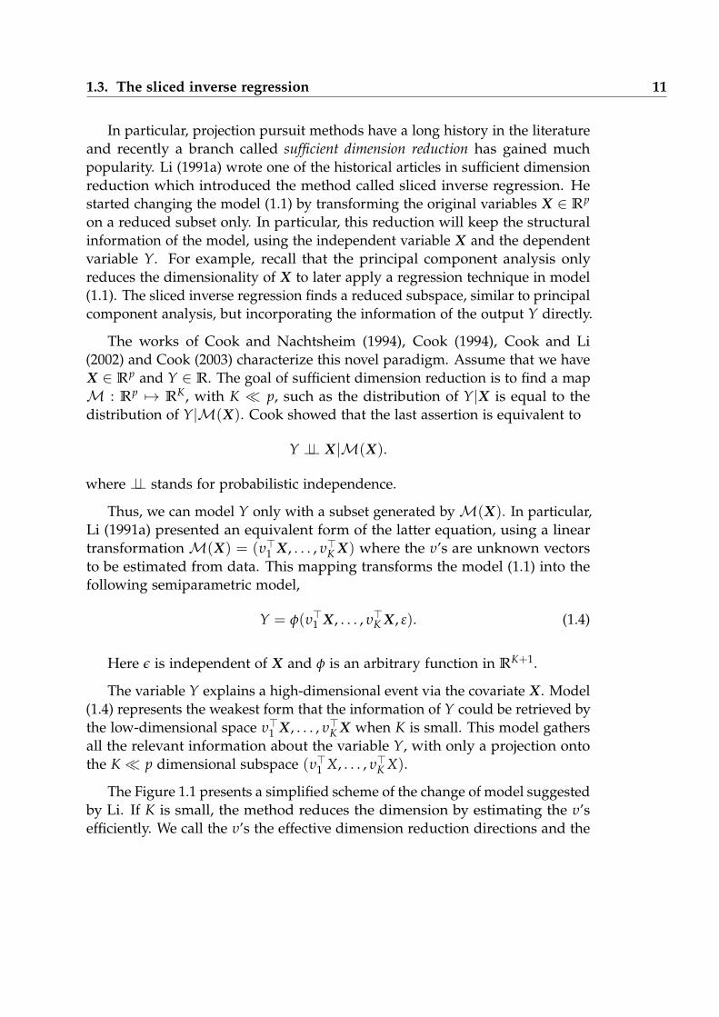
In particular, projection pursuit methods have a long history in the literatureand recently a branch called sufficient dimension reduction has gained muchpopularity. Li (1991a) wrote one of the historical articles in sufficient dimensionreduction which introduced the method called sliced inverse regression. Hestarted changing the model (1.1) by transforming the original variables X ∈ Rp
on a reduced subset only. In particular, this reduction will keep the structuralinformation of the model, using the independent variable X and the dependentvariable Y. For example, recall that the principal component analysis onlyreduces the dimensionality of X to later apply a regression technique in model(1.1). The sliced inverse regression finds a reduced subspace, similar to principalcomponent analysis, but incorporating the information of the output Y directly.
The works of Cook and Nachtsheim (1994), Cook (1994), Cook and Li(2002) and Cook (2003) characterize this novel paradigm. Assume that we haveX ∈ Rp and Y ∈ R. The goal of sufficient dimension reduction is to find a mapM : Rp 7→ RK, with K � p, such as the distribution of Y|X is equal to thedistribution of Y|M(X). Cook showed that the last assertion is equivalent to
Y ⊥⊥ X|M(X).
where ⊥⊥ stands for probabilistic independence.
Thus, we can model Y only with a subset generated byM(X). In particular,Li (1991a) presented an equivalent form of the latter equation, using a lineartransformationM(X) = (υ>1 X, . . . , υ>K X) where the υ’s are unknown vectorsto be estimated from data. This mapping transforms the model (1.1) into thefollowing semiparametric model,
Y = φ(υ>1 X, . . . , υ>K X, ε). (1.4)
Here ε is independent of X and φ is an arbitrary function in RK+1.
The variable Y explains a high-dimensional event via the covariate X. Model(1.4) represents the weakest form that the information of Y could be retrieved bythe low-dimensional space υ>1 X, . . . , υ>K X when K is small. This model gathersall the relevant information about the variable Y, with only a projection ontothe K � p dimensional subspace (υ>1 X, . . . , υ>K X).
The Figure 1.1 presents a simplified scheme of the change of model suggestedby Li. If K is small, the method reduces the dimension by estimating the υ’sefficiently. We call the υ’s the effective dimension reduction directions and the
12 General presentation
Y
m
· · ·X1 Xp
Y
φ
· · ·υ>1 X υ>K X
X1· · · Xp
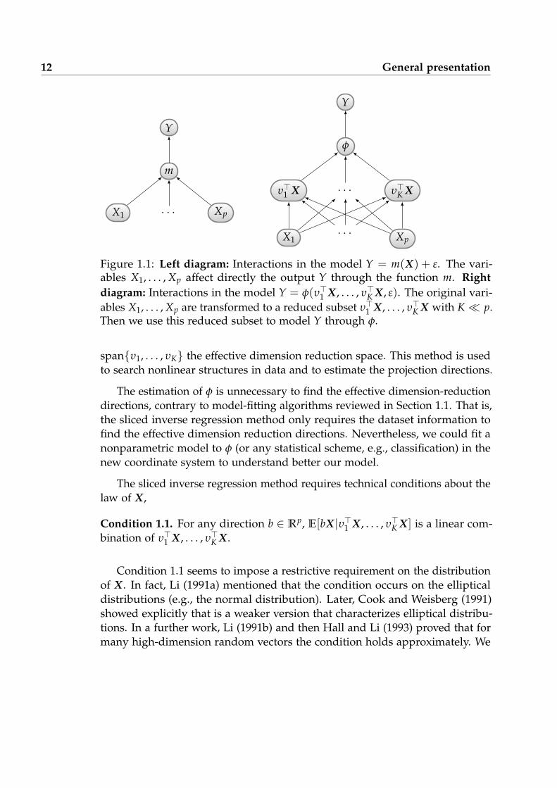
Figure 1.1: Left diagram: Interactions in the model Y = m(X) + ε. The vari-ables X1, . . . , Xp affect directly the output Y through the function m. Rightdiagram: Interactions in the model Y = φ(υ>1 X, . . . , υ>K X, ε). The original vari-ables X1, . . . , Xp are transformed to a reduced subset υ>1 X, . . . , υ>K X with K � p.Then we use this reduced subset to model Y through φ.
span{υ1, . . . , υK} the effective dimension reduction space. This method is usedto search nonlinear structures in data and to estimate the projection directions.
The estimation of φ is unnecessary to find the effective dimension-reductiondirections, contrary to model-fitting algorithms reviewed in Section 1.1. That is,the sliced inverse regression method only requires the dataset information tofind the effective dimension reduction directions. Nevertheless, we could fit anonparametric model to φ (or any statistical scheme, e.g., classification) in thenew coordinate system to understand better our model.
The sliced inverse regression method requires technical conditions about thelaw of X,
Condition 1.1. For any direction b ∈ Rp, E[bX|υ>1 X, . . . , υ>K X] is a linear com-bination of υ>1 X, . . . , υ>K X.
Condition 1.1 seems to impose a restrictive requirement on the distributionof X. In fact, Li (1991a) mentioned that the condition occurs on the ellipticaldistributions (e.g., the normal distribution). Later, Cook and Weisberg (1991)showed explicitly that is a weaker version that characterizes elliptical distribu-tions. In a further work, Li (1991b) and then Hall and Li (1993) proved that formany high-dimension random vectors the condition holds approximately. We

1.3. The sliced inverse regression 13
can ensure Condition 1.1 doing a normal resampling suggested by Brillinger(1991); or averaging the data (by a discrete probability measure) such as they getcloser to an elliptical random vector studied by Cook and Nachtsheim (1994).
We state the following two results in sliced inverse regression.
Theorem 1.1 (Li (1991a)). Under the model (1.4) and Condition 1.1, the centeredinverse regression curve E[X|Y]−E[X] is contained in the linear subspace spannedby υkΣX (k = 1, . . . , K), where ΣX denotes de covariance matrix of X.
Corollary 1.1 (Li (1991a)). Assume that X has been standardized to Z . Under themodel
Y = φ(η>1 Z, . . . , η>K Z, ε)
and Condition 1.1, the standardized inverse regression curve E[Z|Y] is contained inthe linear subspace spanned by ηk = υkΣ1/2
X (k = 1, . . . , K).
Under Condition 1.1, Li showed that the effective dimension reduction spacebelongs to the spectral subspace spanned by Cov(E[Z|Y]). In other words, thecovariance matrix Cov(E[Z|Y]) is degenerated in any direction orthogonal tothe ηk’s. Therefore, the eigenvectors ηk associated with the largest K eigenvaluesof Cov(E[Z|Y]) are the standardized effective dimension reduction directions.
We present the classic sliced inverse regression procedure in the Algorithm1.1. Notice that steps 2 and 3 create an approximation of E[Z|Y] slicing thesupport of Y dividing it in H parts. Using this roughly approximation, the step4 calculates empirically Cov(E[Z|Y]) through a weighted covariance matrix V.Then, it finds the eigenvalues and eigenvectors of V and returns the eigenvectorsassociated to the largest K eigenvalues of the estimated matrix.
We have to emphasize the following result, product from Corollary 1.1 andAlgorithm 1.1:
To find the effective dimension reduction space of model (1.4),it is enough to estimate the matrix Cov(E[Z|Y]). Once this ma-trix is estimated, the eigenvectors associated to the K � p largesteigenvalues of Cov(E[Z|Y]) are the effective dimension reductiondirections.
Summarizing, we will address the high-dimension problem from the suf-ficient dimension reduction point of view. However, the estimation of the

14 General presentation
Algorithm 1.1 Classic sliced inverse regression methodRequire: A sample (Xi, Yi) i = 1, . . . , n.Ensure: υk for k = 1, . . . , K.
1: Standardize X by an affine transformation to get Zi = Σ−1/2X (Xi − X) (i =
1, ..., n), where ΣX and X are the sample covariance matrix and samplemean of X respectively.
2: Divide range of Y into H slices, I1, . . . , IH; let the proportion of the Yi thatfalls in the slice h be ph; that is ph = (1/n)∑n
i=1 δ(Yi), where δ(Yi) takes thevalues 0 or 1 depending on whether Y falls into the h-th slice Ih or not.
3: Within each slice, compute the sample mean of the Zi’s denoted by µh, i.e.,for each h = 1, . . . , H estimate µh = (1/nph)∑y∈Ih
Zi.4: Conduct a (weighted) principal component analysis for the data µh in the
following way: Form the weighted covariance matrix V = ∑Hh=1 phµhµ>h
then find the eigenvalues and the eigenvectors for V.5: Let the K largest eigenvectors (row vectors) be ηk (k = 1, . . . , K). Estimate
υk = ηkΣ−1/2X
empirical covariance matrix is insufficient for this purpose. Therefore, we haveto use another richer object. In particular, we shall use the conditional covari-ance matrix Cov(E[Z|Y]) to solve a connected problem called sliced inverseregression. In particular, we will use the conditional covariance matrix to reducethe dimensionality in problems like nonparametric regression and estimation ofsensitive indices.
1.4 Covariance estimation
The purpose in this thesis will be the estimation of high-dimensional conditionalcovariances. This estimator will be used to reduce the dimensionality onthe nonlinear regression problem (1.1). In Section 1.4.1, we will present abibliographic review of techniques to overcome the dimensionality for thesample covariance matrix ΣX introduced in (1.3). Afterwards, in Section 1.4.2,we will examine some classic approaches for the estimation of conditionalcovariances in the sliced inverse regression context.
1.4.1 High-dimensional covariance estimation
As we mentioned in Section 1.2.3, the estimation of the covariance matrix—orsome related form—is an essential tool for the analysis. The estimator ΣX
1.4. Covariance estimation 15
defined in (1.3) has well known properties as: unbiasedness, consistency, para-metric convergence, among others. However, these properties become uselesswhen the dimension of the model turns high and the empirical covariancematrix has unexpected features.
For example, take a sample from a multivariate Gaussian distributionNp(µ, Σp) where Σp = Ip denotes the identity matrix of size p. If p/n con-verges to some constant c, then the empirical distribution of the eigenvalues ofthe sample covariance matrix Σp follows the Marcenko-Pastur law (Marcenkoand Pastur (1967)), which is supported on ((1−
√c)2, (1 +
√c)2). Therefore, if
the dimension grows faster than the number of observations, the eigenvalueswill be more spread out. Some general references about similar issues in nu-merous contexts are presented in Muirhead (1987), Johnstone (2001), Fan et al.(2008), and references therein.
The authors have proposed solutions to mitigate the irregularities in covari-ance estimation. The general procedure on these situations occurs in two stages:first we need to restrict our attention to “well-behaved” subsets of covariancematrices and then incorporate some regularization into the estimation. Theterm “well-behaved” is vague because it depends on the problem. Sparsity isone common hypothesis on these cases and it seems realistic for real-worldapplications. Another popular matrix class is to assume that the entries of thecovariance decrease at some rate far away of the diagonal.
Roughly speaking, the literature classifies regularized estimation of high-dimensional covariance matrices into two major categories:
Shrinkage type: These estimators shrink the covariance matrix to some well-conditioned one under different performance measures. For instance, Ledoitand Wolf (2004) and Chen et al. (2010) proposed a convex combination betweenΣX and p−1 Tr(ΣX)Ip, with the optimal combination weight that minimizes themean-squared errors. Recently, Fisher and Sun (2011) proposed using diag(ΣX)as the shrinkage target with possibly unequal variances. Other estimators inthis line are: Lam and Fan (2009) minimizes a penalized log-likelihood with aL1-penalty; Meinshausen and Bühlmann (2006) uses Lasso in graph models andLevina et al. (2008) studies a nested Lasso together with a banding techniqueboth to find the structural zeros in sparse covariance matrices.
Matrix transformation type: Estimators in this category operate directly inthe covariance matrix through operators. For instance, thresholding (Bickel
16 General presentation
and Levina (2008a)), banding (Bickel and Levina (2008b)) and tapering (Caiet al. (2010)). When the natural ordering exists in the variables (for example intime-series) the banding and tapering techniques regularize better the empiricalcovariance. The banding sets to zero the elements of the matrix away of somechosen subdiagonal and keep the other entries unchanged. Tapering, improvesthe banding by applying some smoother (originally a linear one) to shrinkgradually the values outside some subdiagonal. We can view banding asa hard-thresholding rule while tapering is a soft-thresholding rule, up to acertain unknown permutation (Bickel and Lindner (2012)). The thresholdingregularization deals with general permutation-invariant covariance matricescutting-off the entries below some level. Assuming certain covariance class ofmatrices, the banding, tapering and thresholding regularizations are statisticalconsistent. In fact, the tapering and thresholding techniques produce optimalrates of convergence (see Cai et al. (2010), Cai et al. (2012) and Cai and Zhou(2012)), contrary to the banding technique (Bickel and Levina (2008b)).
1.4.2 Conditional covariance estimation
The original sliced inverse regression has suffered alternative improvementsthrough the last decades. Recall that the key point in the method is the estima-tion of Cov(E[X|Y]) for X ∈ Rp and Y ∈ R.
Cook and Weisberg (1991) discussed about the validity of Condition 1.1and suggested a variance checking condition. He proposed a new methodcalled sliced average variance estimation (SAVE) using the first two moments ofthe inverse conditional expectation. In particular, they proved that the slicedinverse regression might fail under symmetric models because E[X|Y] could be0. Thus, they suggested the use of Var[X|Y] to recover the effective dimensionreduction directions. Using the same notation as Algorithm 1.1, they proposedthe following estimator
SAVE =H
∑h=1
(I −Var(Z|Y ∈ Ih)),
where I is identity matrix, Z is the standardized version of X and Ih is theindicator for a particular slice h. To estimate Var(Z|Y ∈ Ih) we can use anempirical procedure similar to Algorithm 1.1. Other alternatives to estimatethe conditional variance can be found in Ruppert et al. (1997), Fan (1998) orPérez-González et al. (2010).

1.4. Covariance estimation 17
In a further discussion, Li (1991b) generalized the SAVE estimator usingthat Cov(Z) = Cov(E[Z|Y]) + E[Cov(Z|Y)]. In particular, he defined the SIRIImethod which is represented by the matrix
SIRII = E[(Cov(Z|Y)−E[Cov(Z|Y)])2]
Härdle and Tsybakov (1991) criticized the estimator of the weighted co-variance matrix in step 4 of the Algorithm 1.1. Instead, they considered theestimation of each conditional expectation Ri(Y) = E[Xi|Y] by nonparametricmethods. In other words, the coefficient (i, j) of Cov(E[X|Y]) can be estimatedby
1n
n
∑k=1
Ri(Yk)Rj(Yk). (1.5)
The functions Ri, Rj may be kernel, orthogonal series (e.g., splines, wavelets),or any other estimates. If R is a regressogram, then we get an estimatorsimilar to the sliced inverse regression. Zhu and Fang (1996) showed theasymptotic normality for Cov(E[X|Y]) and its eigenvalues when R is estimatedby the Nadaraya-Watson estimator. Later, Zhu and Yu (2007) proved the exactnormality behavior as Zhu and Fang, but estimating R by a B-splines series. Yinet al. (2010) proposed a recent study on nonparametric conditional covarianceestimation.
Li (1992) presented an application of the Stein lemma (Stein (1981)) to findthe effective dimension reduction space named principal Hessian directions(pHd). He used the average Hessian of E[Y|X] and its eigenvectors to create anew reduced coordinate system. To construct this new space, he applied theStein’s Lemma to find a root-n consistency.
Hsing (1999) estimated Cov(E[X|Y]) by
12n
n
∑k=1
ZkZ>k∗ + Zk∗Z>k
where Zk∗ is the nearest neighbor of Zk. Hsing proved the root-n rate ofconvergence of the new estimator. Cadre and Dong (2010) present a modernreference on the estimation of the central subspaces for dimension reductionusing nearest neighbors.
Bura and Cook (2001) estimated the sliced inverse regression through anadditive parametric form with q elements. Formally, they fixed E[X|Y] to have
18 General presentation
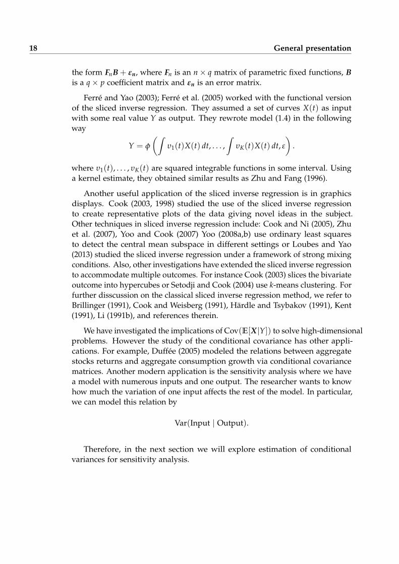
the form FnB + εn, where Fn is an n× q matrix of parametric fixed functions, Bis a q× p coefficient matrix and εn is an error matrix.
Ferré and Yao (2003); Ferré et al. (2005) worked with the functional versionof the sliced inverse regression. They assumed a set of curves X(t) as inputwith some real value Y as output. They rewrote model (1.4) in the followingway
Y = φ
(ˆυ1(t)X(t) dt, . . . ,
ˆυK(t)X(t) dt, ε
).
where υ1(t), . . . , υK(t) are squared integrable functions in some interval. Usinga kernel estimate, they obtained similar results as Zhu and Fang (1996).
Another useful application of the sliced inverse regression is in graphicsdisplays. Cook (2003, 1998) studied the use of the sliced inverse regressionto create representative plots of the data giving novel ideas in the subject.Other techniques in sliced inverse regression include: Cook and Ni (2005), Zhuet al. (2007), Yoo and Cook (2007) Yoo (2008a,b) use ordinary least squaresto detect the central mean subspace in different settings or Loubes and Yao(2013) studied the sliced inverse regression under a framework of strong mixingconditions. Also, other investigations have extended the sliced inverse regressionto accommodate multiple outcomes. For instance Cook (2003) slices the bivariateoutcome into hypercubes or Setodji and Cook (2004) use k-means clustering. Forfurther disscussion on the classical sliced inverse regression method, we refer toBrillinger (1991), Cook and Weisberg (1991), Härdle and Tsybakov (1991), Kent(1991), Li (1991b), and references therein.
We have investigated the implications of Cov(E[X|Y]) to solve high-dimensionalproblems. However the study of the conditional covariance has other appli-cations. For example, Duffée (2005) modeled the relations between aggregatestocks returns and aggregate consumption growth via conditional covariancematrices. Another modern application is the sensitivity analysis where we havea model with numerous inputs and one output. The researcher wants to knowhow much the variation of one input affects the rest of the model. In particular,we can model this relation by
Var(Input | Output).
Therefore, in the next section we will explore estimation of conditionalvariances for sensitivity analysis.

1.5. Sensitivity analysis 19
1.5 Sensitivity analysis
Models are built to approximate or mimic process and systems of differentnature, e.g., physics, economics, chemistry, etc. The mathematical formulationof them, receives a series of equations, parameters, input factors and variablesto generate an output similar to the real process. Some sources of uncertaintyaffect the input variables, such as measurement errors, lack of information orpoor or partial understanding of the system mechanism.
To handle complex models, uncertainty analysis and sensitivity analysis aretwo essential tools. In one hand, uncertainty analysis refers to the determinationof the uncertainty in the outputs that derives from uncertainty in the inputs. Inother hand, sensitivity analysis studies the effects of the variations in the inputson the calculated output. Terms such as influence, importance, ranking anddominance are all related to sensitivity analysis. Ideally, both analysis shouldbe run in tandem.
The model complexity is independent of the model size. A small modelmight have complex interactions hardening its analysis. Instead, Simon (1969)describes the complexity by the numbers of hierarchies, the “span” of each levelin the hierarchy and the number of levels.
Indeed, we can see the sensitivity analysis as a kind of reduction dimensionmethod. While the reduction dimension methods aims to “summarize” thecomplete data space into a lower one, the sensitivity analysis tries to identifythe most relevant inputs in the model according to some score function. Thelarger is the score function for some variable, the larger will be the influence ofthat variable into the model. Below we will review some scores used to identifyrelevant variable in sensitivity analysis. In any case, once we have the new setof relevant variables, we can proceed to do further studies like classification,regression, estimation and so on.
Saltelli et al. (2004) and later Pappenberger et al. (2010), emphasize the im-portance of specifying the objectives before to apply any algorithm or technique.In this way, the scientist knows a priori what it is searching and what kind ofresult he wants. In this way, the most important objectives are
• identify and select the most influent inputs, and identify the nonrelevantones to set them constant,
• map the output behavior with respect to the inputs and focus the analysis
20 General presentation
in some interests zones,
• adjust the model variables taking in account the information of the mostimportant inputs.
Commonly, models in sensitivity analysis ignore the stochastic error. In thisframework, we will assume a nonparametric model similar to equation (1.1),but with ε equal to 0. Therefore, for a set of variables (X1, . . . , Xp) ∈ Rp andY ∈ R we have,
Y = m(X1, . . . , Xp). (1.6)
Also, assume that each X has a valid range of variation and Y is non-null.The explicit form of m is unavailable or simply is hard to obtain. However, theanalyst can create a computer code to describe some phenomenon, includingtwo-phase flow, multi-mode heat transfer, clad oxidation chemistry, stress andstrain, and reactor kinetics. For example, the work of Janon (2012) studies thebehavior of fluids in oceanographic and hydrologic models. Parameters likeviscosity, friction, wind speed, initial height among others, make impossiblehave an explicit equation for the function m. For other illustrations on the useof computer codes, we refer to Oakley and O’Hagan (2004), Langewisch (2010)and references therein.
To solve model (1.6) there exist methods such as: one-at-a-time algorithms,differential analysis, response surface methodology, Monte Carlo proceduresand variance decomposition procedures. Overview of these approaches areavailable in general literature, for instance Saltelli et al. (2000), Christopher Freyand Patil (2002), Helton et al. (2006), Saltelli et al. (2008).
Screening method: These methods are a low computational way to discardfactors in the analysis. For example, we can evaluate the model output byvarying only one variable across its entire range, while fixing the others in theirnominal values. Thus, we measure the difference between the nominal andchanged outputs to extract the most relevant factors. Even if the techniqueis easy to implement, it provides only a limited quantity of information. Forexample, we cannot recover the crossed interactions with this method. For ageneral review in screening we refer to Cullen and Frey (1999), Campolongoet al. (2011) and Saltelli et al. (2009)
Automatic differentiation: If we derivate the output variable with respect toeach factor, we will get a local measure of the model for every variable. In

1.5. Sensitivity analysis 21
general, we want to estimate the following normalized partial derivative,
σXi ∂YσY∂Xi
(1.7)
where σXi and σY are variances of Xi and Y respectively. When the model iscomplex, the estimation of the quantity (1.7) turns hard. Some methods toestimate numerically those partial derivates from a model are available in Rall(1980), Kedem (1980) and Carmichael et al. (1997).
Regression analysis: Recall the classical linear regression,
Y = β0 + β1X1 + · · ·+ βpXp.
We can interpret the regression coefficients βi as the change in the output whenthe in input Xi increase or decreases by one unit (Devore and Peck (1996)). Thisinterpretation is valid if the other factors remain constant. Therefore, we can usethe regression coefficient as nominal measures of the sensitivity in the model.Methods like stepwise regression serve to exclude statistical insignificant inputs.Moreover, we can measure the distance of a linear model and the true using thecoefficient of determination or R2. This coefficient determines the percentage ofvariance in the Y explained by the linear model (see Draper and Smith (1981)).For example, if R2 is equal to 0.9, then the model is 90% linear and one coulduse the β’s for sensitivity analysis at risk of lose 10% of information.
Response surface method: The response surface uses least squared regressionto fit a standardized first- or second-order equation to the data obtained fromthe original model. The amount of time and effort required is as big as thenumber of inputs. For this reason it is recommended to use it only in the lateststeps of the sensitivity investigation. Some general references in the area areMyers et al. (2009) and Goos (2002).
Variance decomposition methods: Fix the variable Xi for some i = 1, . . . , p.Recall that E[Y|Xi] represents the best approximation (in L2) of Y given allthe knowledge of Xi. The variance of E[Y|Xi], with respect Xi, quantifiesthe dispersion of the best approximation of Y. Therefore, when the valueVar(E[Y|Xi]) is large, the variable Xi “influences” more respect to the output Y.In other words, the variation of Y due to the variation of Xi is large. Normalizingthis conditional variance by the total variance of Y, we obtain the first order
22 General presentation
Sobol index associated to Xi,
Si =Var(E[Y|Xi])
Var(Y).
Sobol’ (1993)–inspired by the prior work of Cukier et al. (1978)–initially studiedthe estimation of Si while studying functional decomposition via Monte-Carloprocedures.
We are mainly interested in the variance decomposition methodology ap-plied to sensitivity analysis. In fact, in the next section we will present sometechniques used to estimate the value Si. Additionally, our knowledge in con-ditional covariances, presented in Section 1.4.2, will serve us as a tool for theestimation of Si.
1.5.1 Estimation of Sobol indices
Recall, from the previous Section, the first order Sobol indices of Y associatedto the variables Xi (i = 1, . . . , p) are
Si =Var(E[Y|Xi])
Var(Y)=
E[E[Y|Xi]2]−E[Y]
Var(Y). (1.8)
Given the normalization by Var(Y), each Si belongs to the interval [0, 1]. TheSobol indices measure the relevance of each factor and with respect the output.They represent the percent of the variability of Y when we alter each variable.Thus, Si reveals the sensitivity of Xi with respect to Y. We can define indicestaking account the interactions between the variables. Theoretically, the sum ofall Sobol indices—including interactions—adds up to 1.
Sobol’ (1993) showed that we can decompose any function into terms ofincreasing dimension. We call this kind of decomposition as High-DimensionalModel Representation (HDMR). Li et al. (2001) presents, for example, a completereview about HDMRs. Sobol proved that if each term of the representation hasmean zero and all the term are orthogonal in pairs, then we have the followingequation
Y = ∑i
Vi + ∑ij
Vij + ∑ijk
Vijk + · · ·+ V1,...,p.
whereVi = E[Y|Xi], Vij = E[Y|XiXj]−Vi −Vj, . . .
1.5. Sensitivity analysis 23
In our context, if we take variances in both sides of the HDMR equation, wedefine the higher sensitivity Sobol indices by
Si =Var(E(Y|Xi))
Var(Y)=
Vi
Var(Y), Sij =
Vij
Var(Y), Sijk =
Vijk
Var(Y), · · ·
Finally, we can also define another type of index called Total effects. Thisindex accounts the total contribution to the output variation due to factor Xi,i.e., its first-order effect plus all higher-order effects due to interactions. Definethe variable X∼i as X with the ith factor removed. The total effect index for thevariable Xi is defined by
STi = 1− Var(E[Y|X∼i])
Var(Y).
The aim of this thesis will be the estimation of first-order Sobol indices. Toachieve a good estimate of Si, it is necessary to estimate Var(E[Y|Xi]). The mostdifficult part in equation (1.8) is the term E[E[Y|Xi]
2]. Indeed, the output ofthe model m could be complex and the integrals for the conditional variancecould be intractable analytically. The Monte-Carlo estimation for integrals(Hammersley (1960)) seems to be the simplest but most expensive methodto estimate Si. We start by selecting a set of random points to estimate theinner conditional expectation for a fixed value of Xi. Then, for each of thesevalues make another sample of values to estimate the outer variance. Wesee that as the number of points taken for the evaluation, and the numberof samples increase, the computational complexity of the algorithm increasesas well. Hence, numerous studies have developed numerical approximationssuitable to the practical needs in the applications.
The challenge in this context is given a finite sample, construct a compu-tational effective estimator of Si. Ishigami and Homma (1990) studied one ofthe first solutions in this path. They reduced the computational complexity toonly one Monte-Carlo loop. The idea was to rewrite the Sobol indices Si’s byresampling X and by creating a two-fold function instead of the original. Thistechnique costs only 2p− 1 calculations. Later, Saltelli (2002), found that withn(2p + 2) calculations it could be possible to estimate p− 2 Sobol indices.
The Fourier Amplitude Sensitivity Test (FAST) is another classic method.Cukier et al. (1973) and Cukier et al. (1978) created the FAST which was origi-nally used to analyze sensitivity in nonlinear rate equations. The method was
24 General presentation
developed further by Koda et al. (1979), McRae et al. (1982) and Saltelli et al.(1999). The aim of FAST is to transform a multidimensional integral over all thefactors to a one-dimensional integral. This approach is done using a Fourierexpansion, i.e., we redefine each coefficient as following,
Xi = Gi(sin(wit))
where Gi are suitable transformation functions, {wi} is a set of integer angularfrequencies and t ∈ (−π, π). Some recent investigations with this method canbe found for example in Tarantola et al. (2006) and Tissot and Prieur (2012).
The Sobol pick-freeze (SPF) scheme is widely used and was proposed bySobol’ (1993, 2001). Rewrite the equation (1.8) in the following way,
Si =Cov(Y, Y′)
Var(Y)
whereY′ = m(X′1, X′1, . . . , X′i−1, Xi, X′i+1, . . . , X′p)
and X′j for j 6= i correspond to a random variable independent with the samedistribution as Xj. This scheme freezes the variable of interest while resamplingthe other variables to measure the sensitivity in the former. In SPF we caninterpret the Sobol index as the regression coefficient between the output andits pick-freezed replication. As a Monte-Carlo-based method, SPF requiresthousands of machine computations to get one index. And it gets harder if themodel is created by a complex computer code (e.g., numerical partial differentialequations). To workaround the computational complexity some authors usemeta-models which are—low-fidelity—approximations to the true model. Otherimplementations of the SPF algorithm are proposed in Janon et al. (2013).
Alternatively, Da Veiga and Gamboa (2013) explored another estimator forSobol indices via a Taylor decomposition. As before, the quantity E[E[Y|Xi]
2]represents the hardest part in equation (1.8). They see the conditional expecta-tion as functional depending on the joint distribution f of (X, Y). Specifically,we have the representation
E[E[Y|Xi]2] =
ˆ ( ´xi f (xi, y) dy´f (xi, y) dxi dy
)2
dy.
Using a third order Taylor series development around a preliminary estima-tor of f called f , the latter functional turns into,ˆ
H( f , x, y) f (x, y) dx dy +
ˆK( f , x, y, z) f (x, y) f (x, z) dx dy dz + Γn.
1.6. Thesis scope and outline 25
where H and K are functions depending on f and Γn is an error term.
The Taylor-based estimator has two elements: An empirical estimator forthe first addend; and a projection to some functional orthonormal basis forthe second one. This type of projections were studied for instance by Laurent(1996) in the estimation of integral functionals. They proved that its estimatoris asymptotical normal with variance depending only in the linear part of thefunctional and that it is efficient from the Cramér-Rao point of view.
Further details in sensitivity analysis are in Saltelli et al. (2000), Saltelli et al.(2004) and Saltelli et al. (2008).
1.6 Thesis scope and outline
In Section 1.3, we discussed how the matrix Σ = Cov(E[X|Y]) works intothe sliced inverse regression method. Once we have an estimator for Σ, theeigenvectors associated to the largest eigenvalues of Σ provides an efficientdimension reduction space. In an apparently unrelated issue, we explore,in Section 1.5.1, techniques to estimate sensitivity indices through the valueSi = Var(Y|Xi)/ Var(Y). Both issues identify or extract the real influences ofthe variables into the model and both are based in the estimation of someconditional variance-covariance.
Our work falls in the following chapters:
Chapter 2. Chapter 2 present an Taylor-based estimator inspired by the workof Da Veiga and Gamboa (2013). Motivated by application to sliced inverseregression, we will estimate
σij = E[E[Xi|Y]E[Xj|Y]] for i, j = 1, . . . , p
Notice that this estimator generalizes the Da Veiga and Gamboas’s procedureto three dimensions.
The strategy adopted in this chapter is the following: Denote as f (xi, xj, y)the density function of (Xi, Xj, Y) and fY(y) the marginal density of Y. We canrewrite σij as
σij =
ˆ (´ xi f (xi, xj, y) dxi dxj
fY(y)
)
26 General presentation
(´xj f (xi, xj, y) dxi dxj
fY(y)
)f (xi, xj, y) dxi dxj dy.
We will develop the estimator ΣT = (σij,T)p×p where σij,T is based in theTaylor approximation explained in Section 1.5.1. The asymptotic convergenceof the quadratic part and the error term are negligible with respect to the linearpart. For this reason the variance in the normal distribution is built only by thelinear term.
Summing up, we will prove that the random variable√
n (σij,T − σij)converges to a normal distribution, with mean 0 and variance depending onthe linear part of Tij( f ), when n→ ∞.
Moreover we will show that our estimator is asymptotic efficient using aCramér Rao criterion. Finally, we can extend these results to the whole matrixΣ proving that
√n vech(ΣT − Σ) D−→ N (0, C( f ))
where C = (Cij)p×p depends on the linear part of T( f ) = (Tij( f ))p×p.
Chapter 3. The main issue with the estimator Taylor-based estimator ΣT inChapter 2 is the lack of flexibility to estimate rates of convergence in somegeneral cases. Thus, in Chapter 3 we propose a nonparametric estimator tohandle this issue. If the joint-density function of (X, Y) is smooth enough, wecan achieve parametric rates of convergence. We will use the ideas presented byZhu and Fang (1996).
We will define an estimator of the form (1.5) with Ri, Rj being the Nadaraya-Watson of E[X|Y]. We will call it ΣK. In this work, we will find rates ofconvergence for ΣK depending on the smoothness of the joint distribution f .We will set that f belong to some Hölder functional class with parameters β > 0and radius L > 0.
The main result in Chapter 3 establishes that under some mild conditions andβ ≥ 2, then E[(σij,K − σij)
2] decreases at rate 1/n. In other words, with enoughregularity in the model, we can achieve a parametric rate of convergence with anonparametric estimator. Otherwise, if β < 2, we will get a nonparametric rate.
If p � n, then the estimator ΣK = (σij,K)ij loses its performance. Aswe explain in Section 1.4.1, as the dimension grows, we lose the estimatorconvergence. To recover it, we need to regularize the matrix ΣK assuming

1.6. Thesis scope and outline 27
certain structure in the matrix Σ. We will apply the solution giving by Bickeland Levina (2008b) with a banding method. We shall use the Frobenuis normunder some regular covariance class. Moreover, the rates will depend on thedimensionality and the smoothness of the joint density function f (x, y) andthey will be coherent with the work of Cai et al. (2010). If p� n, we will usethe original covariance matrix ΣK given the low-dimension setting. Otherwise,it is necessary to regularize the estimator to conserve the convergence.
Chapter 4. Finally, we will adjust the nonparametric estimator for condi-tional variances, developed in Chapter 3, to study the quantity E[E[Y|Xi]]for i = 1, . . . , p. We have seen how the latter expectation is related to the estima-tion of the Sobol index Si presented in equation (1.8). Assuming at least that thejoint density of (Xi, Y) is twice times differentiable, we show that the estimatorof Si converges at a parametric rate to Si. Otherwise, for densities with lessthan two derivatives, we obtain a nonparametric rate of convergence depend-ing on the regularity. Our method avoids the run computational expensiveMonte-Carlo simulations because it estimates each Sobol index directly withthe inherent structure of the data. Furthermore, we present some numericalresults with popular sensitivity analysis test models, like the Ishigami function.Our numerical simulations identify correctly the relevant and irrelevant factorsof the models.

Chapter 2
Efficient estimation of conditionalcovariance matrices for dimension
reduction
joint work with S. Da Veiga1 and J-M. Loubes2.
Abstract: Let X ∈ Rp and Y ∈ R. In this chapter we estimate the conditionalcovariance matrix Cov(E[X|Y]) in an inverse regression setting. We develop afunctional Taylor expansion of Cov(E[X|Y]) under some mild conditions. Thismethodology provides a new efficient estimator from the Cramer-Rao point ofview. Also, we study its asymptotic properties.
2.1 Introduction
Consider the nonparametric regression
Yk = ϕ(Xk) + εk k = 1, . . . , n,
where Xk = (X1k, . . . , Xpk) ∈ Rp, Yk ∈ R and εk are random noises withE[εk] = 0. If we face a model with more variables than observed data (i.e.,p� n); the high-dimensional setting blurs the relation between X and Y, unless
1Institut Français du Pétrole, Paris, France.2Institut de Mathématiques de Toulouse, Université Paul Sabatier, Toulouse, France.
29

30 Efficient estimation of conditional covariance matrices
we have at hand a large sample. The literature calls this phenomenon thecurse of dimensionality.
Many authors have studied the dimensionality problem. For instance, thegeneralized linear model in Brillinger (1983), the additive models in Hastie andTibshirani (1990), sparsity constraint models in Li (2007) and references therein.
Alternatively, Li (1991a) propose the sliced inverse regression method. Heconsiders the semiparametric model,
Yk = φ(υ>1 Xk, . . . , υ>K Xk, εk) (2.1)
where the υ’s are unknown vectors in Rp, the εk’s are independent of Xk and φ
is an arbitrary function in RK+1. This model gathers all the relevant informationabout the variable Y, with only a projection onto the K � p dimensionalsubspace (υ>1 X, . . . , υ>K X). If K is small, the method reduces the dimensionby estimating the υ’s efficiently. We call the υ’s effective dimension reductiondirections. This method is also used to search nonlinear structures in data andto estimate the projection directions υ’s.
For a review on the sliced inverse regression methods, we refer to Li (1991a),Li (1991b), Duan and Li (1991) Hardle and Tsybakov (1991) and referencestherein. In short, the eigenvectors associated with the largest eigenvalues ofCov(E[X|Y]) are the model (2.1) effective dimension reduction directions.
In this context, it is enough to estimate Cov(E[X|Y]) to find the effectivedimension reduction directions. Some previous works include: Zhu and Fang(1996) and Ferré and Yao (2003) and Ferré et al. (2005) use kernel estimators;Hsing (1999) combines nearest neighbor and the sliced inverse regression; Buraand Cook (2001) assume that E[X|Y] has some parametric form; Setodji andCook (2004) use k-means and Cook and Ni (2005) write the sliced inverseregression to least square form.
We propose an alternate estimation of the matrix
Cov(E[X|Y]) = E[E[X|Y]E[X|Y]>]−E[X]E[X]>,
using the ideas of Da Veiga and Gamboa (2013), inspired by the prior work ofLaurent (1996). Since we can compute E[X]E[X]> easily, we will focus on theE[E[X|Y]E[X|Y]>] estimation.
We will present a quadratic functional estimator of E[E[X|Y]E[X|Y]>] viaa coordinate-wise Taylor development. Given a preliminary approximation of
2.2. Methodology 31
the (Xi, Xj, Y)’s density, we will make a Taylor’s expansion up to thrice orderof E[E[X|Y]E[X|Y]>]. The first order term drives the asymptotic convergencemeanwhile the other ones rest negligible. We will also prove this kind ofconvergence for the whole matrix. Besides, we shall prove also its efficiency ina semiparametric framework using a Cramer-Rao criterion.
Instead of compete with the methods mentioned before, we intent to makeit complementary. Indeed, we offer an alternative method on plug-in methodsfor conditional covariance matrices with minimum variance properties.
We organize this chapter as follows. Section 2.2 motivates our investigationof Cov(E[X|Y]) using a Taylor approximation. In Section 2.3.1 we set up allthe notations and hypotheses. We demonstrate, in Section 2.3.2, the efficientconvergence of each coordinate for our estimator. Also, we state the asymptoticnormality for the whole matrix. For the quadratic term of the Taylor’s expansionof Cov(E[X|Y]), we find an asymptotic bound for the variance in Section 2.4.We postpone all the technical Lemmas and related proofs to Sections 2.6.2 and2.6.1 respectively.
2.2 Methodology
Let X ∈ Rp be a squared integrable random vector with p ≥ 1 and Y ∈ R be arandom variable. Denote as Xi, Xj the i-th and j-th coordinates of X, respectivelyfor i and j different. We denote by fij(xi, xj, y) the joint density of the vector(Xi, Xj, Y) for i, j = 1 . . . p. Remark that the density function fij depends onthe indices i and j, namely for each triplet (Xi, Xj, Y) there exist a joint densityfunction called fij(xi, xj, y). For the sake of simplicity, we will denote fij only byf to avoid cumbersome notations. When i is equal to j, we will call to the jointdensity of (Xi, Y) by fi(xi, y) , for i = 1, . . . , p. When the context is clear, we canname fi simply by f . Finally, let fY(·) =
´R
f (xi, xj, ·) dxi dxj be the marginaldensity function with respect to Y
The studies of Laurent (1996) and Da Veiga and Gamboa (2013) have alreadyconsidered the estimation of the diagonal of Cov(E[X|Y]). According to theparagraph precedent, they assumed a context where the indices i and j are equal.The former studied the estimation of density integrals in the unidimensionalcase and the latter applied this estimation into sensibility analysis for computingSobol indices. In this work, we shall extend their methodologies to the case idifferent of j to find an alternative estimator for the sliced inverse regressiondirections.

32 Efficient estimation of conditional covariance matrices
Recall that
Σ = Cov(E[X|Y]) = E[E[X|Y]E[X|Y]>]−E[X]E[X]>,
where A> means the transpose of A. We can easily estimate E[X] with theempirical sample mean. Also, without loss of generality, we always can assumethe variables X centered, i.e., E[X] = 0.
Define each entry of the conditional covariance matrix Σ as
σij = E[E[Xi|Y]E[Xj|Y]] i, j = 1, . . . , p.
Given a sample of (X, Y), we aim to study the asymptotic and efficiency prop-erties of σij. Also, we will find similar results for the whole matrix Σ.
Notice that we can write each σij for i 6= j as
σij =
ˆ (´ xi f (xi, xj, y) dxi dxj
fY(y)
)(´
xj f (xi, xj, y) dxi dxj
fY(y)
)f (xi, xj, y) dxi dxj dy. (2.2)
We will need the following functional operator.
Definition 2.1. Let ψ be a square-integrable function in L2(dxi dxj, dy). Definethe functional mapping ψ 7→ Tij(ψ) where
Tij(ψ) =
ˆ (´ xiψ(xi, xj, y) dxi dxj´ψ(xi, xj, y) dxi dxj
)(´
xjψ(xi, xj, y) dxi dxj´ψ(xi, xj, y) dxi dxj
)ψ(xi, xj, y) dxi dxj dy. (2.3)
A word to clarify the notations it is necessary at this point. The functionalTij(ψ) takes any squared-integrable ψ an estimates the value described inequation (2.3). If we take specifically ψ = f , then the functional Tij( f ) is equalto the parameter σij defined in 2.2. We will apply a Taylor development toTij( f ) to obtain an estimator for σij. Thus, we should be able of transfer all theproperties of Tij( f ) to σij.
2.2. Methodology 33
Suppose that (Xik, Xjk, Yk), k = 1, . . . , n is an independent and identicallydistributed sample of (Xi, Xj, Y). Assume that f is a preliminary estimator of festimated with a subsample of size n1 < n. The main idea is to expand Tij( f )in a Taylor’s series around a neighborhood of f .
More precisely, define an auxiliar function F : [0, 1]→ R;
F(u) = Tij(u f + (1− u) f )
with u ∈ [0, 1]. The Taylor’s expansion of F between 0 and 1 up to the thirdorder is
F(1) = F(0) + F′(0) +12
F′′(0) +16
F′′′(ξ)(1− ξ)3 (2.4)
for some ξ ∈ [0, 1]. Moreover, we have
F(1) = Tij( f )
F(0) = Tij( f )
To simplify the notations set
mi( fu, y) =
´xi fu(xi, xj, y) dxi dxj´
fu(xi, xj, y) dxi dxj,
where fu = u f + (1− u) f , for all u belonging to [0, 1]. Notice that if u = 0 thenmi( f0, y) = mi( f , y).
We can rewrite F(u) as
F(u) =ˆ
mi( fu, y)mj( fu, y) fu(xi, xj, y) dxi dxj dy.
The next Proposition gives the Tij( f ) Taylor’s expansion.
Proposition 1 (Linearization of the operator T). For the functional Tij( f ) definedin (2.3), the following decomposition holds
Tij( f ) =ˆ
H1( f , xi, xj, y) f (xi, xj, y) dxi dxj dy
+
ˆH2( f , xi1, xj2, y) f (xi1, xj1, y) f (xi2, xj2, y) dxi1 dxj1 dxi2 dxj2 dy + Γn (2.5)
where
H1( f , xi, xj, y) = ximj( f , y) + xjmi( f , y)−mi( f , y)mj( f , y)
34 Efficient estimation of conditional covariance matrices
H2( f , xi1, xj2, y) =1´
f (xi, xj, y) dxi dxj(xi1 −mi( f , y))(xj2 −mj( f , y))
Γn =16
F′′′(ξ)(1− ξ)3, (2.6)
for some ξ ∈]0, 1[.
This decomposition separates Tij( f ) in three parts. A linear functionalof f —which is easily estimable—, a quadratic one and an error term Γn. InSection 2.3.2, we prove that the term H1 drives the asymptotic convergence ofTij( f ). Besides, Theorem 2.2 gives the semiparametric efficiency. We control thequadratic functional variance in Section 2.4.
2.3 Main Results
In this section we estimate σij efficiently employing decomposition (2.5). Sincewe used n1 < n to build a preliminary approximation f , we will use a sampleof size n2 = n− n1 to estimate σij. Since the first term in equation (2.5) is alinear functional in f , then its empirical estimator is
1n2
n2
∑k=1
H1( f , Xik, Xjk, Yk). (2.7)
Conversely, the second addend complicates the estimate because it is anonlinear functional of f . However, in Section 2.4 we will study deeply thegeneral functional
θ( f ) =ˆ
η(xi1, xj2, y) f (xi1, xj1, y) f (xi2, xj2, y)dxi1dxj1dxi2dxj2dy
where η : R3 → R is a bounded function. The value θn of θ( f ) gives anapproximation of the second term in (2.5). This technique extends the methoddeveloped by Da Veiga and Gamboa (2013).
2.3.1 Hypothesis and Assumptions
Throughout the chapter, we will use the following notations. Let ak and bk fork = 1, 2, 3 be real numbers where ak < bk. Let, for i and j fixed, L2( dxi dxj dy) bethe squared integrable functions in the cube [a1, b1]× [a2, b2]× [a3, b3]. Moreover,

2.3. Main Results 35
let (pl(xi, xj, y))l∈D be an orthonormal basis of L2( dxi dxj dy), where D is asubset of {1, . . . , p}. Let al =
´pl f denote the scalar product of f with pl.
Furthermore, denote by L2( dxi dxj) (resp. L2( dy)) the set of squared in-tegrable functions in [a1, b1]× [a2, b2] (resp. [a3, b3]). If
(αlα(xi, xj)lα∈D1
)(resp.(
βlβ(y)lβ∈D2
)) is an orthonormal basis of L2( dxi dxj) (resp. L2( dy)) then pl(xi, xj, y) =
αlα(xi, xj)βlβ(y) with l = (lα, lβ) ∈ D1 × D2.
We also use the following subset of L2( dxi dxj dy)
E =
{∑l∈D
el pl : (el)l∈D is such that ∑l∈D
∣∣∣∣ elcl
∣∣∣∣2 < 1
}
where (cl)l∈D is a decreasing fixed sequence.
Moreover assume that (Xi, Xj, Y) have a bounded joint density fij on [a1, b1]×[a2, b2]× [a3, b3] which lies in the ellipsoid E .
Besides, XnD−→X (resp. Xn
P−→X) denotes the convergence in distribution orweak convergence (resp. convergence in probability) of Xn to X. Additionally, wedenote by supp f the support of f .
Let (Mn)n≥1 denote a sequence of subsets of D. For each n there exists Mnsuch that Mn ⊂ D. Write by |Mn| the cardinal of Mn. We shall make three mainassumptions:
Assumption 2.1. For all n ≥ 1 there is a subset Mn ⊂ D such that
supl /∈Mn
|cl|2 ≈√|Mn|/n
(An ≈ B means λ1 ≤ An/Bn ≤ λ2 for some positives constants λ1 and λ2). Moreover,for all f ∈ L2( dx dy dz),
´(SMn f − f )2 dx dy dz→ 0 when n→ ∞, where SMn f =
∑l∈Mn al pl.
Assumption 2.2. We assume that supp f ⊂ [a1, b1]× [a2, b2]× [a3, b3] and for all(x, y, z) ∈ supp f , 0 < α ≤ f (x, y, z) ≤ β with α, β ∈ R.
Assumption 2.3. It is possible to find an estimator f of f built with n1 ≈ n/ log (n)observations, such that for ε > 0,
∀(x, y, z) ∈ supp f , 0 < α− ε ≤ f (x, y, z) ≤ β + ε

36 Efficient estimation of conditional covariance matrices
and,∀ 2 ≤ q ≤ +∞, ∀l ∈N∗, E f ‖ f − f ‖l
q ≤ C(q, l)n−lλ1
for some λ > 1/6 and some constant C(q, l) not depending on f belonging to theellipsoid E .
Assumption 2.1 is necessary to bound the bias and variance of θn. It dependson n to obtain a good quadratic approximation of the density projection usingonly Mn coefficients. This condition relates the growing size of the set Mn withthe decay rate of the sequence cl.This behavior relates strongly the smoothnessof the density function f with the size of the coefficients cl.
For instance, we will use the Example 2 in Laurent (1996) and its notation.Assume that f belongs to some Hölder space with index greater than s. If thewavelet ψ has regularity r > s, then f ∈ E where
E =
∑j≥0
∑λ∈Λj
α(λ)ψλ, ∑j≥0
∑λ∈Λj
22js|α(λ)|2 ≤ 1
.
See Meyer and Salinger (1993) for further details.
Moreover, they show that if s > p/4 and
Mn ={
λ ∈ Λj, j ≤ j0, 2j0 = n2/(p+4s)}
then supl /∈Mn|cl|2 ≈
√|Mn|/n. Also, |Mn|/n→ 0 with
|Mn| ≈ n2p/(d+4s), supl /∈Mn
|cl|2 ≈ 2−2j20 = n−4s/(p+4s).
Assumption 2.2 and 2.3 establish that Γn = O(1/n), i.e., the error term in(2.5) is negligible. In Assumption 2.3, the function f converges faster than somegiven rate. Of course, the existence of such an estimator deeply relies on theregularity of the true function.
On the one hand, a large literature exists to determine which estimator wehave to choose to achieve a rate of convergence for some kind of functions. Seefor instance Tsybakov (2009). On the other hand, suppose we set a class ofestimators and a rate of convergence. Another type of theory specify the kindof functions that we might approximate with these estimators and achieving
2.3. Main Results 37
this convergence rate. Particularly, the maxiset theory and we refer to Autinet al. (2009) or Kerkyacharian and Picard (2002) for general articles.
The Nikol’skii functional class provides an example for our framework.For x ∈ Rp, s > 0 and L > 0, we consider the class Hq(s, L) of Nikol’skii offunctions f ∈ Lq( dx) with partials derivatives up to order r = bsc inclusive.For each of these derivatives f (r), we assume that
‖ f (r)(·+ h)− f (r)(·)‖q ≤ L|hs−r| ∀h ∈ R.
If f ∈ Hq(s, L) with s > p/4, then Assumption 2.3 is satisfied (see Ibragimovand Khas’ minskii (1983, 1984)).
2.3.2 Efficient Estimation of σij
We consider the following estimator of σij adopting the decomposition of Tij( f )in equation (2.5) along equations (2.7) and (2.12),
σij,T =1n2
n2
∑k=1
H1(
f , Xik, Xjk, Yk)+
1n2(n2 − 1) ∑
l∈M
n2
∑k 6=k′=1
pl(Xik, Xjk, Yk
)ˆ
pl(xi, xj, Yk′
)H3(
f , xi, xj, Xik′ , Xjk′ , Yk′)
dxi dxj
− 1n2(n2 − 1) ∑
l,l′∈M
n2
∑k 6=k′=1
pl(Xik, Xjk, Yk
)pl′(Xik′ , Xjk′ , Yk′
)ˆ
pl(xi1, xj1, y
)pl′(xi2, xj2, y
)H2(
f , xi1, xj2, y)
dxi1 dxj1 dxi2 dxj2dy. (2.8)
where H3( f , xi1, xj1, xi2, xj2, y) = H2( f , xi1, xj2, y) + H2( f , xi2, xj1, y) and n2 =n− n1. We remove the term Γn of (2.5) in equation (2.8) because we will provethat it is negligible compared to the others terms.
Notice that if we take for example n1 = n/ log n, then n1/n → 0 andn2/n → 1 as n → ∞. Thus, we will use n instead of n2 (asymptoticallyspeaking) from this point to simplify the notation.
The next theorem gives the asymptotic behavior of σij,T for i and j.
Theorem 2.1. Let Assumptions 2.1-2.3 hold and |Mn|/n→ 0 when n→ ∞. Then,
√n(σij,T − σij
) D−→ N (0, Cij( f )), (2.9)
38 Efficient estimation of conditional covariance matrices
andlim
n→∞n E[σij,T − σij]
2 = Cij( f ), (2.10)
whereCij( f ) = Var(H1( f , Xi, Xj, Y))
The asymptotic variance of σij depends only on H1( f , Xi, Xj, Y). In otherwords, the linear part of (2.5) controls the asymptotic normality of σij. Thisproperty entails the natural efficiency of σij,T.
The next theorem produces the σij’s semiparametric Cramér-Rao bound.
Theorem 2.2 (Semiparametric Cramér Rao bound). Consider the estimation of
σij = E[E[Xi|Y]E[Xj|Y]>]
for a random vector (Xi, Xj, Y) with joint density f ∈ E .
Let f0 ∈ E be a density verifying the assumptions of Theorem 2.1. Then, for anyestimator σij,T of σij and every family {Vr( f0)}r>0 of neighborhoods of f0 we have
inf{Vr( f0)}r>0
lim infn→∞
supf∈Vr( f0)
n E f[σij,T − σij
]2 ≥ Cij( f0)
where Vr( f0) = { f : ‖ f − f0‖2 < r} for r > 0.
Theorems 2.1 and 2.2 establish the asymptotic efficiency of the estimatorσij,T defined in (2.8).
We have proved asymptotic normality entry by entry of the matrix Σ =(σij)p×p using the estimator ΣT = (σij,T)p×p defined in equation (2.8). To extendthe result to the whole matrix, we introduce the half-vectorization operator vech.This operator stacks only the columns from the principal diagonal of a squarematrix downwards in a column vector. Formally, for a p× p matrix A = (aij),
vech(A) =[a11, · · · , ap1, a22, · · · , ap2, · · · , a33, · · · , app
]> .
Name H1( f ) the matrix with entries defined by(
H1( fij, xi, xj, y))
i,j if i differentof j and (H1( fi, xi, xi, y))i,i when i is equal to j and i, j = 1, . . . , p.
Corollary 2.1 generalizes our previous results.

2.4. Estimation of quadratic functionals 39
Corollary 2.1. Let Assumptions 2.1-2.3 hold and |Mn|/n→ 0 when n→ ∞. ThenTn has the following properties:
√n vech(ΣT − Σ) D−→ N (0, C( f )),
limn→∞
n E
[vech
(ΣT − Σ
)vech
(ΣT − Σ
)>]= C( f )
where the limit is taking element-wise and
C( f ) = Cov(vech(H1( f ))).
The estimator σij,T is asymptotically normal with a variance depending onthe linear term of the Taylor development. Given this particular nature, it waspossible to show the asymptotic efficiency of σij,T. It means, among all theestimators of σij, the estimator defined in equation (2.8) has the lowest variance.The conclusions in Theorems 2.1 and 2.2 depend on to estimate accurately thequadratic term of σij,T. We will handle this issue in the next section.
2.4 Estimation of quadratic functionals
We have proved, in Section 2.3.2, the asymptotic normality and found an efficientsemiparametric Cramér-Rao bound of the estimator σij,T defined in equation(2.8). We used the Taylor decomposition (2.5) to construct the estimator σij,T. Inthe present section, we will build an estimator for the quadratic term
ˆH2( f , xi1, xj2, y) f (xi1, xj1, y) f (xi2, xj2, y) dxi1 dxj1 dxi2 dxj2 dy.
To this end, we build a general estimator of the parameter with the form:
θ =
ˆη(xi1, xj2, y) f (xi1, xj1, y) f (xi2, xj2, y) dxi1 dxj1 dxi2 dxj2 dy,
for f ∈ E and η : R3 → R a bounded function.
Given M = Mn a subset of D, consider the estimator
θn =1
n(n− 1) ∑l∈M
n
∑k 6=k′=1
pl(Xik, Xjk, Yk)
ˆpl(xi, xj, Yk′)
(η(xi, Xjk′ , Yk′) + η(Xik′ , xj, Yk′)
)dxi dxj

40 Efficient estimation of conditional covariance matrices
− 1n(n− 1) ∑
l,l′∈M
n
∑k 6=k′=1
pl(Xik, Xjk, Yk)pl′(Xik′ , Xjk′ , Yk′)
ˆpl(xi1, xj1, y)pl′(xi2, xj2, y)η(xi1, xj2, y) dxi1 dxj1 dxi2 dxj2 dy. (2.11)
To simplify the presentation of Theorem 2.1, write ψ(xi1, xj1, xi1, xj2, y) =η(xi1, xj2, y) + η(xi2, xj1, y) verifying
ˆψ(xi1, xj1, xi2, xj2, y) dxi1 dxj1 dxi2 dxj2dy
=
ˆψ(xi2, xj2, xi1, xj1, y) dxi1 dxj1 dxi2 dxj2 dy.
With this notation we can simplify (2.11) into
θn =1
n(n− 1) ∑l∈M
n
∑k 6=k′=1
pl(Xik, Xjk, Yk)
ˆpl(xi, xj, Yk′)ψ(xi, xj, Xik′ , Xjk′ , Yk′) dxi dxj
− 1n(n− 1) ∑
l,l′∈M
n
∑k 6=k′=1
pl(Xik, Xjk, Yk)pl′(Xik′ , Xjk′ , Yk′)
ˆpl(xi1, xj1, y)pl′(xi2, xj2, y)η(xi1, xj2, y) dxi1 dxj1 dxi2 dxj2 dy. (2.12)
The bias of θ is equal to
−ˆ(SM f (xi1, xj1, y)− f (xi1, xj1, y))(SM f (xi2, xj2, y)− f (xi2, xj2, y))
η(xi1, xj2, y) dxi1 dxj1 dxi2 dxj2 dy.
The following Theorem gives an explicit bound for the θn variance.
Theorem 2.3. Let Assumption 2.1 hold. Then if |Mn|/n→ 0 when n→ ∞, then θnhas the following property∣∣∣n E
[(θn − θ
)2]−Λ( f , η)∣∣∣ ≤ γ
[|Mn|
n+ ‖SMn f − f ‖2 + ‖SMn g− g‖2
],

2.5. Conclusion 41
where g(xi, xj, y) =´
f (xi2, xj2, y)ψ(xi, xj, xi2, xj2, y) dxi2 dxj2 and
Λ( f , η) =
ˆg(xi, xj, y)2 f (xi, xj, y) dxi dxj dy
−(ˆ
g(xi, xj, y) f (xi, xj, y) dxi dxj dy)2
,
where γ is constant depending only on ‖ f ‖∞, ‖η‖∞, and ∆ = (b1 − a1)× (b2 − a2).Moreover, this constant is an increasing function of these quantities.
Note that equation (2.3) implies that
limn→∞
n E[(θn − θ)2] = Λ( f , η).
We can control the quadratic term of σij,T, which is a particular case of θ
choosing η(xi1, xj2, y) = H2( f , xi1, xj2, y).
We will show, in proof 2.6.1, that Λ( f , η)→ 0 when n→ ∞. Consequently,the linear part of σij,T governs its asymptotic variance, yielding also asymptoticefficiency.
2.5 Conclusion
In this chapter, we propose a new way to estimate Cov(E[X|Y]), different fromthe usual plugin type estimators. We use a general functional Tij( f ) dependingon the joint density function f of (Xi, Xj, Y). In particular, we grab a suitableapproximation f of f and construct a coordinate-wise Taylor’s expansion upto order three around it. We call this estimator σij,T. This expansion serves toestimate Cov(E[X|Y]) using an orthonormal base of L2( dxi dxj dy).
We highlight that σij,T is asymptotic normal with variance leaded by the firstorder term. This behavior also causes an efficiency from the Cramér-Rao’s pointof view. Again, the Cramér-Rao bound depends only on the linear part of theTaylor’s series.
With the help of the vech operator, we expanded our results to the matrix-estimator Σ formed with the entries σij,T. We showed that the T( f )’s linear termguides the variance for the ΣT’s asymptotic normality.
Even if we aim principally to study a new class of estimators for Cov(E[X|Y]),we refer to Da Veiga and Gamboa (2013) for some simulations in a context simi-lar to ours. In general, their numerical result behaves reasonably well despite its

42 Efficient estimation of conditional covariance matrices
implementation’s complexity. These results could also work in our frameworkand we will consider them in a future article.
The estimator ΣT could have negative eigenvalues, violating the semipositivedefiniteness of the covariance. From a practical point of view, we could projectΣT into the space of positive-semidefinite matrices. It means, we first diagonalizeΣT and then replace negative eigenvalues by 0. The resulting estimator isthen semipositive-definite. The works of Bickel and Levina (2008a,b), andCai et al. (2010), present an extended discussion about techniques on matrixregularization.
This research constitutes a first step in the study of estimators based inTaylor’s series with minimum variance. To simplify the implementation’scomplexity of this estimator, we will explore another kind of techniques likenonparametric methods for example.
2.6 Appendix
2.6.1 Proofs
Proof of Proposition 1.
We need to calculate the three first derivatives of F(u). to ease the calculation,notice first that
ddu
mi( fu, y)u =
´ (xi −mi( fu, y)
)( f (xi, xj, y)− f (xi, xj, y)) dxi dxj´fu(xi, xj, y) dxi dxj
. (2.13)
It is possible to interchange the derivate with the integral sign because fand f are bounded. Now, using (2.13) and taking u = 0 we have
F′(0) =ˆ [
ximj( f , y) + xjmi( f , y)−mi( f , y)mj( f , y)]
( f (xi, xj, y)− f (xi, xj, y)) dxi dxj dy. (2.14)
Deriving mi( fu, y)mj( fu, y) using the same arguments as in (2.13) and againtaking u = 0 we get,
2.6. Appendix 43
F′′(0) =ˆ
2´f (xi, xj, y) dxi dxj
(xi1 −mi( f , y))(xj2 −mj( f , y))( f (xi1, xj1, y)− f (xi1, xj1, y))
( f (xi2, xj2, y)− f (xi2, xj2, y)) dxi1 dxj1 dxi2 dxj2 dy. (2.15)
Using the previous arguments we find also that
F′′′(u) =ˆ −6´
fu(xi, xj, y)dxidxj
(xi1 −mj( fu, y)
)(xj2 −mj( fu, y)
)(
f (xi1, xj1, y)− f (xi1, xj1, y))(
f (xi2, xj2, y)− f (xi2, xj2, y))(
f (xi3, xj3, y)− f (xi3, xj3, y))
dxi1 dxj1 dxi2 dxj2 dxi3 dxj3 dy (2.16)
Replacing (2.14), (2.15) and (2.16) into (2.4) we get the desired decomposition.
Proof of Theorem 2.1. We will first control the remaining term (2.6),
Γn =16
F′′′(ξ)(1− ξ)3.
Remember that
F′′′(ξ) = −6ˆ (
xi1 −mi( fξ , y)) (
xj2 −mj( fξ , y))(´
fξ(xi, xj, y) dxi dxj)2(
f (xi1, xj1, y)− f (xi1, xj1, y)) (
f (xi2, xj2, y)− f (xi2, xj2, y))
(f (xi3, xj3, y)− f (xi3, xj3, y)
)dxi1 dxj1 dxi2 dxj2 dxi3 dxj3 dy,
Assumptions 2.1 and 2.2 ensure that the first part of the integrand is boundedby a constant µ. Furthermore,
|Γn| ≤ µ
ˆ ∣∣∣ f (xi1, xj1, y)− f (xi1, xj1, y)∣∣∣ ∣∣∣ f (xi2, xj2, y)− f (xi2, xj2, y)
∣∣∣∣∣∣ f (xi3, xj3, y)− f (xi3, xj3, y)∣∣∣ dxi1 dxj1 dxi2 dxj2 dxi3 dxj3 dy
= µ
ˆ (ˆ ∣∣∣ f (xi, xj, y)− f (xi, xj, y)∣∣∣ dxi dxj
)3
dy
≤ µ∆3ˆ ∣∣∣ f (xi, xj, y)− f (xi, xj, y)
∣∣∣3 dxi dxj dy
44 Efficient estimation of conditional covariance matrices
by the Hölder inequality. Then E[Γ2n] is equal to O(E‖ f − f ‖6
3). Since f verifiesAssumption 2.3, this quantity is of order O(n−6λ
1 ). Since we also assume n1 ≈n/ log(n) and λ > 1/6, then n−6λ
1 = o (1/n). Therefore, we get E[Γ2n] = o(1/n)
which implies that the remaining term Γn is negligible.
To prove the asymptotic normality of σij,T, we shall show that√
n(σij,T − Tij( f )
)and
Z(n)ij =
1n2
n2
∑k=1
H1(
f , Xik, Xjk, Yk)−ˆ
H1( f , xi, xj, y) f (xi, xj, y)) dxi dxj dy (2.17)
have the same asymptotic behavior. We can get for Z(n)ij a classic central limit
theorem with variance
Cij( f ) = Var(H1( f , xi, xj, y))
=
ˆH1( f , xi, xj, y)2 f (xi, xj, y)) dxi dxj dy
−(ˆ
H1( f , xi, xj, y) f (xi, xj, y) dxi dxj dy)2
which implies (2.9) and (2.10). In order to establish our claim, we will showthat
R(n)ij =
√n[σij,T − Tij( f )− Z(n)
ij
](2.18)
has second-order moment converging to 0.
Define Z(n)ij as Z(n)
ij with f replaced by f . Let us note that R(n)ij = R1 + R2
where
R1 =√
n[σij,T − Tij( f )− Z(n)
ij
]R2 =
√n[
Z(n)ij − Z(n)
ij
].
It only remains to state that E[R21] and E[R2
2] converges to 0. We can rewrite R1as
R1 = −√
n[
Q−Q + Γn
]

2.6. Appendix 45
with
Q =
ˆH2( f , xi1, xj2, y) f (xi1, xj1, y) f (xi2, xj2, y) dxi1 dxj1 dxi2 dxj2 dy
H2( f , xi1, xj2, y) =1´
f (xi, xj, y) dxi dxj
(xi1 −mi( f , y)
) (xj2 −mj( f , y)
).
We can estimate H2( f , xi1, xj2, y) = η(xi1, xj2, y) as done in Section 2.4. LetQ the estimator of Q. Since E[Γ2
n] = o(1/n), we only have to control theterm
√n(Q−Q) which is such that limn→∞ n E[Q−Q]2 = 0 by Lemma 2.7 in
Section 2.6.2 below. This Lemma implies that E[R21]→ 0 as n→ ∞. For R2 we
have
E[R22] =
nn2
[ˆ (H1( f , xi, xj, y)− H1( f , xi, xj, y)
)2f (xi, xj, y)) dxi dxj dy
]− n
n2
[ˆH1( f , xi, xj, y) f (xi, xj, y)) dxi dxj dy
−ˆ
H1( f , xi, xj, y)2 f (xi, xj, y)) dxi dxj dy]
2.
The same arguments as the ones of Lemma 2.7 (mean value and Assumptions2.2 and 2.3) show that E[R2
2]→ 0.
Proof of Theorem 2.2 . To prove the inequality we will use the usual frameworkdescribed in Ibragimov and Khas’Minskii (1991). The first step is to calculatethe Fréchet derivative of Tij( f ) at some point f0 ∈ E . Assumptions 2.2 and 2.3and equation (2.5), imply that
Tij( f )− Tij( f0) =
ˆ (ximj( f0, y) + xjmi( f0, y)−mi( f0, y)mj( f0, y)
)(
f (xi, xj, y)− f0(xi, xj, y))
dxi dxj dy + O(ˆ
( f − f0)2)
where mi( f0, y) =´
xi f0(xi, xj, y) dxi dxj dy/´
f0(xi, xj, y) dxi dxj dy. Therefore,the Fréchet derivative of Tij( f ) at f0 is T′ij( f0) · h = 〈H1( f0, ·), h〉 with
H1( f0, xi, xj, y) = ximj( f0, y) + xjmi( f0, y)−mi( f0, y)mj( f0, y).
Using the results of Ibragimov and Khas’Minskii (1991), denote
H( f0) ={
u ∈ L2( dxi dxj dy),´
u(xi, xj, y)√
f0(xi, xj, y) dxi dxj dy = 0}
the set

46 Efficient estimation of conditional covariance matrices
of functions in L2( dxi dxj dy) orthogonal to√
f0, PH( f0) the projection onto
H( f0), An(t) =(√
f0)
t/√
n and P(n)f0
the joint distribution of(Xik, Xjk
)k =
1, . . . , n under f0. Since(Xik, Xjk
)k = 1, . . . , n are i.i.d., the family
{P(n)
f0, f ∈ E
}is differentiable in quadratic mean at f0 and therefore locally asymptoticallynormal at all points f0 ∈ E in the direction H( f0) with normalizing factorAn( f0) (see the details in Van der Vaart (2000)). Then, by the results ofIbragimov and Khas’Minskii (1991) say that under these conditions, denot-
ing Kn = Bnθ′( f0)AnPH( f0) with Bn =√
nu, if KnD−→ K and if K(u) = 〈t, u〉,
then for every estimator σij,T of Tij( f ) and every family V( f0) of vicinities of f0,we have
inf{V( f0)}
lim infn→∞
supf∈V( f0)
n E[σij,T − Tij( f0)]2 ≥ ‖tL2( dxi dxj dy)‖2.
Here,
Kn(u) =√
nT′( f0) ·√
f0√n
PH( f0)(u) = T′( f0)
(√f0
(u−
√f0
ˆu√
f0
)),
since for any u ∈ L2( dxi dxj dy) we can write it as u =√
f0⟨√
f0, u⟩+
PH( f0)(u). In this case Kn(u) does not depend on n and
K(h) = T′( f0) ·(√
f0
(u−
√f0
ˆh√
f0
))=
ˆH1( f0, ·)
√f0u−
ˆH1( f0, ·)
√f0
ˆu√
f0
= 〈t, u〉
with
t(xi, xj, y) = H1( f0, xi, xj, y)√
f0 −(ˆ
H1( f0, xi, xj, y) f0
)√f0.
The semi-parametric Cramér-Rao bound for this problem is thus
‖tL2( dxi, dxj, dy)‖ =ˆ
H1( f0, xi, xj, y)2 f0 dxi dxj dy
−(ˆ
H1( f0, xi, xj, y) f0 dxi dxj dy)2
and we recognize the expression Cij( f0) found in Theorem 2.1.

2.6. Appendix 47
Proof of Corollary 2.1. The proof is based in the following observation. Em-ploying equation (2.18) we have
Tn − T( f ) = Zn( f ) +Rn√
n
where Zn( f ) and Rn are matrices with elements Z(n)ij and R(n)
ij , defined in (2.17)and (2.18), respectively.
Hence we have,
n E
[∥∥∥vech(
Tn − T( f )− Zn( f ))∥∥∥2
]= E
[‖vech (Rn)‖2
]= ∑
i≤jE
[(R(n)
ij
)2]
.
We see by Lemma 2.7 that E[R2ij]→ 0 as n→ 0. It follows that
n E[‖vech(
Tn − T( f )− Zn( f ))‖2]→ 0 as n→ 0.
We know that if Xn, X and Yn are random variables, then if XnD−→ X and
(Xn −Yn)P−→ 0, follows that Yn
D−→ X.
Remember also that convergence in L2 implies convergence in probability,therefore √
n vech(
Tn − T( f )− Zn( f )) P−→ 0.
By the multivariate central limit theorem we have that√
n vech (Zn( f )) D−→N (0, C( f )). Therefore,
√n vech
(Tn − T( f )
) D−→ N (0, C( f )).
Proof of Theorem 2.3. For abbreviation, we write M instead of Mn and setm = |Mn|. We first compute the mean squared error of θn as
E[θn − θ]2 = Bias2(θn) + Var(θn)
where Bias(θn) = E[θn]− θ.
We begin the proof by bounding Var(θn). Let A and B be m× 1 vectors withcomponents
al =
ˆpl(xi, xj, y) f (xi, xj, y) dxi dxj dy l = 1, . . . , m,

48 Efficient estimation of conditional covariance matrices
bl =
ˆpl(xi1, xj1, y) f (xi2, xj2, y)ψ(xi1, xj1, xi2, xj2, y) dxi1 dxj1 dxi2 dxj2 dy
=
ˆpl(xi, xj, y)g(xi, xj, y) dxi dxj dy l = 1, . . . , m
where g(xi, xj, y) =´
f (xi2, xj2, y)ψ(xi, xj, xi2, xj2, y) dxi2 dxj2. Let Q and R bem× 1 vectors of centered functions
ql(xi, xj, y) = pl(xi, xj, y)− al
rl(xi, xj, y) =ˆ
pl(xi2, xj2, y)ψ(xi, xj, xi2, xj2, y) dxi2 dxj2 − bl
for l = 1, . . . , m. Let C a m×m matrix of constants with indices l, l′ = 1, . . . , mdefined by
cll′ =
ˆpl(xi1, xj1, y)pl′(xi2, xj2, y)η(xi1, xj2, y) dxi1 dxj1 dxi2 dxj2 dy.
Let us denote by Un the process
Unh =1
n(n− 1)
n
∑k 6=k′=1
h(Xik, Xjk, Yk, Xik′ , Xjk′ , Yk′
)and Pn the empirical measure
Pnh =1n
n
∑k=1
h(Xik, Xjk, Yk
)for some h in L2( dxi, dxj, dy). With these notations, θn has the Hoeffding’sdecomposition
θn =1
n(n− 1) ∑l∈M
n
∑k 6=k′=1
(ql(Xik, Xjk, Yk) + al
)(rl(Xik′ , Xjk′ , Yk′) + bl
)− 1
n(n− 1) ∑l,l′∈M
n
∑k 6=k′=1
(ql(Xik, Xjk, Yk) + al
)(ql′(Xik′ , Xjk′ , Yk′) + al′
)cll′
= UnK + PnL + A>B− A>CA
where
K(xi1, xj1, y1, xi2, xj2, y2
)=Q>(xi1, xj1, y1)R(xi2, xj2, y2)
−Q>(xi1, xj1, y1)CQ(xi2, xj2, y2)
2.6. Appendix 49
L(xi, xj, y) =A>R(xi, xj, y) + BQ(xi, xj, y)− 2A>CQ(xi, xj, y).
Therefore Var(θn) = Var(UnK) + Var(PnL) − 2 Cov(UnK, PnL). These threeterms are bounded in Lemmas 2.2 - 2.4, which gives
Var(θn) ≤20
n(n− 1)‖η‖2
∞‖ f ‖2∞∆2(m + 1) +
12n‖η‖2
∞‖ f ‖2∞∆2.
For n enough large and a constant γ ∈ R,
Var(θn) ≤ γ‖η‖2∞‖ f ‖2
∞∆2(
mn2 +
1n
).
The term Bias(θn) is easily computed, as proven in Lemma 2.5, is equal to
−ˆ (
SM f (xi1, xj1, y)− f (xi1, xj1, y)) (
SM f (xi2, xj2, y)− f (xi2, xj2, y))
η(xi1, xj1, xi2, xj2, y) dxi1 dxj1 dxi2 dxj2 dy.
From Lemma 2.5, we bound the bias of θn by
|Bias(θn)| ≤ ∆‖η‖∞ supl /∈M|cl|2.
The assumption of(
supl /∈M |ci|2)2≈ m/n2 and since m/n→ 0, we deduce that
E[θn − θ]2 has a parametric rate of convergence O (1/n).
Finally to prove (2.3), note that
n E[θn − θ]2 = n Bias2(θn) + n Var(θn)
= n Bias2(θn) + n Var(UnK) + n Var(PnL).
We previously proved that for some λ1, λ2 ∈ R
n Bias2(θn) ≤ λ1∆2‖η‖2∞
mn
n Var(UnK) ≤ λ2∆2‖ f ‖2∞‖η‖2
∞mn
.
Thus, Lemma 2.6 implies
|n Var(PnL)−Λ( f , η)| ≤ λ [‖SM f − f ‖2 + ‖SMg− g‖2] ,
where λ is an increasing function of ‖ f∞‖2, ‖η‖2∞ and ∆. From all this we
deduce (2.3) which ends the proof of Theorem 2.3.

50 Efficient estimation of conditional covariance matrices
2.6.2 Technical Results
Lemma 2.1 (Bias of θn). The estimator θn defined in (2.12) estimates θ with bias equalto
−ˆ (
SM f (xi1, xj1, y)− f (xi1, xj1, y)) (
SM f (xi2, xj2, y)− f (xi2, xj2, y))
η(xi1, xj2, y) dxi1 dxj1 dxi2 dxj2 dy.
Proof. Let θn = θ1n − θ2
n where
θ1n =
1n(n− 1) ∑
l∈M∑
k 6=k′=1pl(Xik, Xjk, Yk)
ˆpl(xi, xj, Yk′)ψ(xi, xj, Xik′ , Xjk′ , Yk′)dxidxj
θ2n = − 1
n(n− 1) ∑l,l′∈M
n
∑k 6=k′=1
pl(Xik, Xjk, Yk)pl′(Xik′ , Xjk′ , Yk′)
ˆpl(xi1, xj1, y)pl′(xi2, xj2, y)η(xi1, xj2, y) dxi1 dxj1 dxi2 dxj2 dy.
Let us first compute E[θ1n].
E[θ1n]
= ∑l∈M
ˆpl(xi1, xj1, y) f (xi1, xj1, y) dxi1 dxj1 dy
ˆpl(xi1, xj1, y)ψ(xi1, xj1, xi2, xj2, y) f (xi2, xj2, y) dxi1 dxj1 dxi2 dxj2 dy
= ∑l∈M
al
ˆpl(xi1, xj1, y)ψ(xi1, xj1, xi2, xj2, y) f (xi2, xj2, y) dxi1 dxj1 dxi2 dxj2 dy
=
ˆ (∑
l∈Mal pl(xi2, xj2, y)
)ψ(xi1, xj1, xi2, xj2, y) f (xi2, xj2, y) dxi1 dxj1 dxi2 dxj2 dy
=
ˆSM f (xi1, xj1, y) f (xi2, xj2, y)η(xi1, xj2, y) dxi1 dxj1 dxi2 dxj2 dy
+
ˆSM f (xi2, xj2, y) f (xi1, xj1, y)η(xi1, xj2, y) dxi1 dxj1 dxi2 dxj2 dy
Now for θ2n, we get
E[θ2n]

2.6. Appendix 51
= ∑l,l′∈M
ˆpl(xi, xj, y) f (xi, xj, y) dxi dxj dy
ˆpl′(xi, xj, y) f (xi, xj, y) dxi dxj dy
ˆpl(xi1, xj1, y)pl′(xi2, xj2, y)η(xi1, xj2, y) dxi1 dxj1 dxi2 dxj2 dy
= ∑l,l′∈M
alal′
ˆpl(xi1, xj1, y)pl′(xi2, xj2, y)η(xi1, xj2, y) dxi1 dxj1 dxi2 dxj2 dy
=
ˆ (∑
l∈Mal pl(xi1, xj1, y)
)(∑
l′∈Mal′ pl′(xi2, xj2, y)
)η(xi1, xj2, y) dxi1 dxj1 dxi2 dxj2 dy
=
ˆSM f (xi1, xj1, y)SM f (xi2, xj2, y)η(xi1, xj2, y) dxi1 dxj1 dxi2 dxj2 dy.
Arranging these terms and using
Bias(θn) = E[θn]− θ = E[θ1n]−E[θ2
n]− θ
we obtain the desire bias.
Lemma 2.2 (Bound of Var(UnK)). Under the assumptions of Theorem 2.3, we have
Var(UnK) ≤ 20n(n− 1)
‖η‖2∞‖ f ‖2
∞∆2(m + 1)
Proof. Note that UnK is centered because Q and R are centered and (Xik, Xjk, Yk),k = 1, . . . , n is an independent sample. So Var(UnK) is equal to
E[UnK]2 =E
(1
(n(n− 1))2
n
∑k1 6=k′1=1
n
∑k2 6=k′2=1
K(Xik1 , Xjk1 , Yk1 , Xik′1
, Xjk′1, Yk′1
)K(Xik2 , Xjk2 , Yk2 , Xik′2
, Xjk′2, Yk′2
))
=1
n(n− 1)E
(K2(Xi1, Xj1, Y1, Xi2, Xj2, Y2
)+ K
(Xi1, Xj1, Y1, Xi2, Xj2, Y2
)K(Xi2, Xj2, Y2, Xi1, Xj1, Y1
))
By the Cauchy-Schwarz inequality, we get
Var(UnK) ≤ 2n(n− 1)
E[K2 (Xi1, Xj1, Y1, Xi2, Xj2, Y2)].
52 Efficient estimation of conditional covariance matrices
Moreover, using the fact that 2|E[XY]| ≤ E[X2] + E[Y2], we obtain
E[K2 (Xi1, Xj1, Y1, Xi2, Xj2, Y2)]
≤ 2
[E[(Q>(Xi1, Xj1, Y1)R(Xi2, Xj2, Y2)
)2]
+ E[(Q>(Xi1, Xj1, Y1)CQ(Xi2, Xj2, Y2)
)2]
].
We will bound these two terms. The first one is
E[(Q>(Xi1, Xj1, Y1)R(Xi2, Xj2, Y2)
)2]
= ∑l,l′∈M
(ˆpl(xi, xj, y)pl′(xi, xj, y) f (xi, xj, y) dxi dxj dy− alal′
)(ˆ
pl(xi2, xj2, y)pl′(xi3, xj3, y)ψ(xi1, xj1, xi2, xj2, y)
ψ(xi1, xj1, xi3, xj3, y) f (xi1, xj1, y) dxi1 dxj1 dxi2 dxj2 dxi3 dxj3 dy− blbl′
)=W1 −W2 −W3 + W4
where
W1 =
ˆ∑
l,l′∈Mpl(xi1, xj1, y)pl′(xi1, xj1, y)
pl(xi2, xj2, y′)pl′(xi3, xj3, y′)ψ(xi4, xj4, xi2, xj2, y′)
ψ(xi4, xj4, xi3, xj3, y′) f (xi1, xj1, y)
f (xi4, xj4, y′) dxi1 dxj1 dxi2 dxj2 dxi3 dxj3 dxi4 dxj4 dy dy′
W2 =
ˆ∑
l,l′∈Mblbl′ pl(xi1, xj1, y)pl′(xi1, xj1, y) f (xi1, xj1, y) dxi1 dxj1dy
W3 =
ˆ∑
l,l′∈Malal′ pl(xi2, xj2, y′)pl′(xi3, xj3, y′)
ψ(xi4, xj4, xi2, xj2, y′)ψ(xi4, xj4, xi3, xj3, y′)
f (xi4, xj4, y′) dxi2 dxj2 dxi3 dxj3 dxi4 dxj4 dy′
W4 = ∑l,l′∈M
alal′blbl′ .
W2 and W3 are positive, hence
E[(
2Q>(Xi1, Xj1, Y1)R(Xi2, Xj2, Y2))2] ≤W1 + W4.
2.6. Appendix 53
W1 =
ˆ∑
l,l′∈Mpl(xi1, xj1, y)pl′(xi1, xj1, y)
(ˆpl(xi2, xj2, y′)ψ(xi4, xj4, xi2, xj2, y′) dxi2 dxj2
)(ˆ
pl′(xi3, xj3, y′)ψ(xi4, xj4, xi3, xj3, y′) dxi3 dxj3
)f (xi1, xj1, y) f (xi4, xj4, y′) dxi1 dxj1 dxi4 dxj4 dy dy′
≤ ‖ f ‖2∞ ∑
l,l′∈M
ˆpl(xi1, xj1, y)pl′(xi1, xj1, y) dxi1 dxj1dy
ˆ (ˆpl(xi2, xj2, y′)ψ(xi4, xj4, xi2, xj2, y′) dxi2 dxj2
)(ˆ
pl′(xi3, xj3, y′)ψ(xi4, xj4, xi3, xj3, y′) dxi3 dxj3
)dxi2 dxj2 dxi4 dxj4 dy′
Since pl’s are orhonormal we have
W1 ≤‖ f ‖2∞ ∑
l∈M
ˆ (ˆpl(xi2, xj2, y′)ψ(xi4, xj4, xi2, xj2, y′) dxi2 dxj2
)2
dxi4 dxj4 dy′.
Moreover by the Cauchy-Schwarz inequality and ‖ψ‖∞ ≤ 2‖η‖∞(ˆpl(xi2, xj2, y′)ψ(xi4, xj4, xi2, xj2, y′) dxi2 dxj2
)2
≤ˆ
pl(xi2, xj2, y′)2 dxi2 dxj2
ˆψ(xi4, xj4, xi2, xj2, y′)2 dxi2 dxj2
≤ ‖ψ‖2∞∆ˆ
pl(xi2, xj2, y′)2 dxi2 dxj2
≤ 4‖η‖2∞∆ˆ
pl(xi2, xj2, y′)2 dxi2 dxj2,
and thenˆ (ˆ
pl(xi2, xj2, y′)ψ(xi4, xj4, xi2, xj2, y′) dxi2 dxj2
)2dxi4 dxj4 dy′
≤ 4‖η‖2∞∆2ˆ
pl(xi2, xj2, y′)2 dxi2 dxj2 dy′
= 4‖η‖2∞∆2.

54 Efficient estimation of conditional covariance matrices
Finally,W1 ≤ 4‖η‖2
∞‖ f ‖2∞∆2m.
For the term W4 using the facts that SM f and SMg are projection and that´f = 1, we have
W4 =
(∑
l∈Malbl
)2
≤ ∑l∈M
a2l ∑
l∈Mb2
l ≤ ‖ f ‖22‖g‖2
2 ≤ ‖ f ‖∞‖g‖22.
By the Cauchy-Schwartz inequality we have ‖g‖22 ≤ 4‖η‖2
∞‖ f ‖∞∆2 and then
W4 ≤ 4‖η‖2∞‖ f ‖2
∞∆2
which leads to
E[(Q>(Xi1, Xj1, Y1)R(Xi2, Xj2, Y2)
)2] ≤ 4‖η‖2
∞‖ f ‖2∞∆2(m + 1). (2.19)
The second term E[(Q>(Xi1, Xj1, Y1CQ(Xi2, Xj2, Y2)
)] = W5 − 2W6 + W7 where
W5 =
ˆ∑l1,l′1
∑l2,l′2
cl1l′1cl2l′2
pl1(xi1, xj1, y)pl2(xi1, xj1, y)pl′1(xi2, xj2, y′)pl′2
(xi2, xj2, y′)
f (xi1, xj1, y) f (xi2, xj2, y′) dxi1 dxj1 dxi2 dxj2 dy′ dy
W6 =
ˆ∑l1,l′1
∑l2,l′2
cl1l′1cl2l′2
al1 al2 pl′1(xi, xj, y)pl′2
(xi, xj, y) dxi dxj dy
W7 = ∑l1,l′1
∑l2,l′2
cl1l′1cl2l′2
al1 al′1al2 al′2
.
Using the previous manipulation, we show that W6 ≥ 0. Thus
E[(Q>(Xi1, Xj1, Y1)CQ(Xi2, Xj2, Y2)
)] ≤W5 + W7.
First, observe that
W5 = ∑l1,l′1
∑l2,l′2
cl1l′1cl2l′2
(ˆpl1(xi1, xj1, y)pl2(xi1, xj1, y) f (xi1, xj1, y) dxi1 dxj1 dy
)(ˆ
pl′1(xi2, xj2, y′)pl′2
(xi2, xj2, y′) f (xi2, xj2, y′) dxi2 dxj2 dy′)
≤‖ f ‖2∞ ∑
l1,l′1
∑l2,l′2
cl1l′1cl2l′2
(ˆpl1(xi1, xj1, y)pl2(xi1, xj1, y) dxi1 dxj1 dy
)

2.6. Appendix 55
(ˆpl′1
(xi2, xj2, y′)pl′2(xi2, xj2, y′) dxi2 dxj2 dy′
)=‖ f ‖2
∞ ∑l,l′
c2ll′
again using the orthonormality of the pl’s. Besides given the decompositionpl(xi, xj, y) = αlα(xi, xj)βlβ
(y),
∑l,l′
c2ll′ =
ˆ∑lβ,l′β
βlβ(y)βl′β
(y)βlβ(y′)βl′β
(y′)
∑lα,l′α
(ˆαlα(xi1, xj1)αl′α(xi2, xj2)η(xi1, xj2, y) dxi1 dxj1 dxi2 dxj2
)(ˆ
αlα(xi3, xj3)αl′α(xi4, xj4)η(xi3, xj4, y′) dxi3 dxj3 dxi4 dxj4
)dydy′
But
∑lα,l′α
(ˆαlα(xi1, xj1)αl′α(xi2, xj2)η(xi1, xj2, y) dxi1 dxj1 dxi2 dxj2
)(ˆ
αlα(xi3, xj3)αl′α(xi4, xj4)η(xi3, xj4, y′) dxi3 dxj3 dxi4 dxj4
)= ∑
lα,l′α
ˆαlα(xi1, xj1)αl′α(xi2, xj2)η(xi1, xj2, y)αlα(xi3, xj3)
αl′α(xi4, xj4)η(xi3, xj4, y′) dxi1 dxj1 dxi2 dxj2 dxi3 dxj3 dxi4 dxj4
=
ˆ∑lα
(ˆαlα(xi1, xj1)η(xi1, xj2, y) dxi1 dxj1
)αlα(xi3, xj3)
∑l′α
(ˆαl′α(xi4, xj4)η(xi3, xj4, y′) dxi4 dxj4
)αl′α(xi2, xj2) dxi2 dxj2 dxi3 dxj3
≤ˆ
η(xi3, xj3, xi2, xj2, y)η(xi3, xj2, y′) dxi2 dxj2 dxi3 dxj3
≤ ∆2‖η‖2∞
using the orthonormality of the basis αlα . Then we get
∑l,l′
c2ll′ ≤ ∆2‖η‖2
∞
ˆ ∑lβ,l′β
βlβ(y)βl′β
(y)βlβ(y′)βl′β
(y′) dy dy′

56 Efficient estimation of conditional covariance matrices
= ∆2‖η‖2∞ ∑
lβ,l′β
(ˆβlβ
(y)βl′β(y) dy
)2
≤ ∆2‖η‖2∞ ∑
lβ
(ˆβ2
lβ(y) dy
)2
≤ ∆2‖η‖2∞m
since the βlβare orthonormal. Finally
W5 ≤ ‖ f ‖2∞‖η‖2
∞∆2m.
Now for W7 we first will bound,
|∑l,l′
cll′alal′ | = |ˆ
∑l,l′∈M
alal′ pl2(xi1, xj1, y)pl′1(xi2, xj2, y)η(xi1, xj2, y) dxi1 dxj1 dxi2 dxj2 dy|
≤ˆ|SM(xi1, xj1, y)SM(xi2, xj2, y)η(xi1, xj2, y)| dxi1 dxj1 dxi2 dxj2 dy
≤ ‖η‖∞
ˆ (ˆ|SM(xi1, xj1, y)SM(xi2, xj2, y)| dy
)dxi1 dxj1 dxi2 dxj2.
Taking squares in both sides and using the Cauchy-Schwartz inequality twice,we get(
∑l,l′
cll′alal′
)2
= ‖η‖2∞
(ˆ (ˆ|SM(xi1, xj1, y)SM(xi2, xj2, y)| dy
)dxi1 dxj1 dxi2 dxj2
)2
≤ ‖η‖2∞∆2ˆ (ˆ
|SM(xi1, xj1, y)SM(xi2, xj2, y)| dy)2
dxi1 dxj1 dxi2 dxj2
≤ ‖η‖2∞∆2ˆ (ˆ
SM(xi1, xj1, y)2 dy)(ˆ
SM(xi2, xj2, y′)2 dy′)
dxi1 dxj1 dxi2 dxj2
= ‖η‖2∞∆2ˆ
SM(xi1, xj1, y)2SM(xi1, xj1, y′)2 dxi1 dxj1 dxi2dxj2 dy dy′
= ‖η‖2∞∆2
(ˆSM(xi, xj, y)2 dxi dxj dy
)≤ ‖η‖2
∞∆2‖ f ‖2∞.
Finally,
E[(Q>(Xi1, Xj1, Y1)CQ(Xi2, Xj2, Y2)
)2] ≤ ‖η‖2
∞‖ f ‖2∞∆2(m + 1). (2.20)
2.6. Appendix 57
Collecting (2.19) and (2.20), we obtain
Var(UnK) ≤ 20n(n− 1)
‖η‖2∞‖ f ‖2
∞∆2(m + 1)
which concludes the proof of Lemma 2.2.
Lemma 2.3 (Bound for Var(PnL)). Under the assumptions of Theorem 2.3, we have
Var(PnL) ≤ 12n‖η‖2
∞‖ f ‖2∞∆2.
Proof. First note that given the independence of(Xik, Xjk, Yk
)k = 1, . . . , n we
haveVar(PnL) =
1n
Var(L(Xi1, Xj1, Y1
))
we can write L(Xi1, Xj1, Y1
)as
A>R(Xi1, Xj1, Y1
)+ B>Q
(Xi1, Xj1, Y1
)− 2A>CQ
(Xi1, Xj1, Y1
)= ∑
l∈Mal
(ˆpl(xi, xj, Y1)ψ(xi, xj, Xi1, Xj1, Y1) dxi dxj − bl
)+ ∑
l∈Mbl(
pl(Xi1, Xj1, Y1)− al)− 2 ∑
l,l′∈Mcll′al′
(pl(Xi1, Xj1, Y1)− al
)=
ˆ∑
l∈Mal pl(xi, xj, Y1)ψ(xi, xj, Xi1, Xj1, Y1) dxi dxj
+ ∑l∈M
bl pl(Xi1, Xj1, Y1)− 2 ∑l,l′∈M
cll′al′ pl(Xi1, Xj1, Y1)− 2AtB− 2AtCA.
=
ˆSM f (xi, xj, Y1)ψ(xi, xj, Xi1, Xj1, Y1) dxi dxj + SMg(Xi1, Xj1, Y1)
− 2 ∑l,l′∈M
cll′al′ pl(Xi1, Xj1, Y1)− 2A>B− 2A>CA.
Let h(xi, xj, y) =´
SM f (xi2, xj2, y)ψ(xi, xj, xi2, xj2, y) dxi2 dxj2, we have
SMh(xi, xj, y) = ∑l∈M
(ˆh(xi2, xj2, y)pl(xi2, xj2, y) dxi2 dxj2 dy
)pl(xi, xj, y)
= ∑l∈M
(ˆSM f (xi3, xj3, y)ψ(xi2, xj2, xi3, xj3, y)
pl(xi2, xj2, y) dxi2 dxj2 dxi3 dxj3 dy)
pl(xi, xj, y)
58 Efficient estimation of conditional covariance matrices
= ∑l,l′∈M
(ˆal′ pl′(xi3, xj3, y)ψ(xi2, xj2, xi3, xj3, y)
pl(xi2, xj2, y) dxi2 dxj2 dxi3 dxj3 dy)
pl(xi, xj, y)
= 2 ∑l,l′∈M
(ˆal′ pl′(xi3, xj3, y)η(xi2, xj3, y)
pl(xi2, xj2, y) dxi2 dxj2 dxi3 dxj3 dy)
pl(xi, xj, y)
= 2 ∑l,l′∈M
al′cll′ pl(xi, xj, y)
and we can write
L(Xi1, Xj1, Y1
)= h
(Xi1, Xj1, Y1
)+ SMg
(Xi1, Xj1, Y1
)− SMh
(Xi1, Xj1, Y1
)− 2A>B− 2A>CA.
Thus,
Var(L(Xi1, Xj1, Y1
))
= Var(h(Xi1, Xj1, Y1
)+ SMg
(Xi1, Xj1, Y1
)+ SMh
(Xi1, Xj1, Y1
))
≤ E[(h(Xi1, Xj1, Y1
)+ SMg
(Xi1, Xj1, Y1
)+ SMh
(Xi1, Xj1, Y1
))2]
≤ E[(h(Xi1, Xj1, Y1
))2+(SMg
(Xi1, Xj1, Y1
))2+(SMh
(Xi1, Xj1, Y1
))2].
Each of these terms can be bounded
E[(h(Xi1, Xj1, Y1
))2]
=
ˆ (ˆSM f (xi2, xj2, y)ψ(xi1xj2, xi2, xj2, y) dxi2 dxj2
)2
f (xi1, xj1, y) dxi1 dxj1 dy
≤ ∆ˆ
SM f (xi2, xj2, y)2ψ(xi1xj2, xi2, xj2, y)2 f (xi1, xj1, y) dxi1 dxj1 dxi2 dxj2 dy
≤ 4∆2‖ f ‖∞‖η‖2∞
ˆSM f (xi, xj, y)2 dxi dxj dy
= 4∆2‖ f ‖∞‖η‖2∞‖SM f ‖2
2
≤ 4∆2‖ f ‖∞‖η‖2∞‖ f ‖2
2
≤ 4∆2‖ f ‖2∞‖η‖2
∞
and similar calculations are valid for the others two terms,
E[(SMg
(Xi1, Xj1, Y1
))2] ≤ ‖ f ‖∞‖SMg‖2
2 ≤ ‖ f ‖∞‖g‖22 ≤ 4∆2‖ f ‖2
∞‖η‖2∞
2.6. Appendix 59
E[(SMh
(Xi1, Xj1, Y1
))2] ≤ ‖ f ‖∞‖SMh‖2
2 ≤ ‖ f ‖∞‖h‖22 ≤ 4∆2‖ f ‖2
∞‖η‖2∞.
Finally we get,
Var(PnL) ≤ 12n‖η‖2
∞‖ f ‖2∞∆2.
Lemma 2.4 (Computation of Cov(UnK, PnL)). Under the assumptions of Theorem2.3, we have
Cov(UnK, PnL) = 0.
Proof of Lemma 2.4. Since UnK and PnL are centered, we have
Cov(UnK, PnL)= E[UnKPnL]
= E
[1
n2(n− 1)
n
∑k 6=k′=1
K(Xik, Xjk, Yk, Xik′ , Xjk′ , Yk′
) n
∑k=1
L(Xik, Xjk, Yk
)]
=1n
E[K(Xi1, Xj1, Y1, Xi2, Xj2, Y2
)(L(Xi1, Xj1, Y1
)+ L
(Xi2, Xj2, Y2
))]
=1n
E[(
Q>(Xi1, Xj1, Y1)R(Xi2, Xj2, Y2)−Q>(Xi1, Xj1, Y1)CQ(Xi2, Xj2, Y2))
(A>R(Xi1, Xj1, Y1) + B>Q(Xi1, Xj1, Y1)− 2A>CQ(Xi1, Xj1, Y1)
+ A>R(Xi2, Xj2, Y2) + B>QXi2, Xj2, Y2)− 2A>CQ(Xi2, Xj2, Y2))]
= 0.
Since K, L, Q and R are centered.
Lemma 2.5 (Bound of Bias(θn)). Under the assumptions of Theorem 2.3, we have
|Bias(θn)| ≤ ∆‖η‖∞ supl /∈M|cl|2.
Proof.
|Bias θn| ≤ ‖η‖∞
ˆ (ˆ|SM f (xi1, xj1, y)− f (xi1, xj1, y)| dxi1 dxj1
)(ˆ|SM f (xi2, xj2, y)− f (xi2, xj2, y)| dxi2 dxj2
)dy
60 Efficient estimation of conditional covariance matrices
= ‖η‖∞
ˆ (ˆ|SM f (xi, xj, y)− f (xi, xj, y)| dxi dxj
)2
dy
≤ ∆‖η‖∞
ˆ (SM f (xi, xj, y)− f (xi, xj, y)
)2 dxi dxj dy
= ∆‖η‖∞ ∑l,l′/∈M
alal′
ˆpl(xi, xj, y)pl′(xi, xj, y) dxi dxj dy
= ∆‖η‖∞ ∑l /∈M|al|2 ≤ ∆‖η‖∞ sup
l /∈M|cl|2.
We use the Hölder’s inequality and the fact that f ∈ E then ∑l /∈M |al|2 ≤supl /∈M |cl|2.
Lemma 2.6 (Asymptotic variance of√
n(
PnL).). Under the assumptions of Theorem
2.3, we haven Var(PnL)→ Λ( f , η)
where
Λ( f , η) =
ˆg(xi, xj, y)2 f (xi, xj, y) dxi dxj dy
−(ˆ
g(xi, xj, y) f (xi, xj, y) dxi dxj dy)2
.
Proof. We proved in Lemma 2.3 that
Var(L(Xi1, Xj1, Y1
))
= Var(h(Xi1, Xj1, Y1
)+ SMg
(Xi1, Xj1, Y1
)+ SMh
(Xi1, Xj1, Y1
))
= Var(A1 + A2 + A3)
=3
∑k,l=1
Cov(Ak, Al).
We claim that ∀k, l ∈ {1, 2, 3}2, we have∣∣∣∣∣Cov(Ak, Al)
− εkl
[ˆg(xi, xj, y)2 f (xi, xj, y) dxi dxj dy−
(ˆg(xi, xj, y) f (xi, xj, y) dxi dxj dy
)2]∣∣∣∣∣
≤ λ [‖SM f − f ‖2 + ‖SMg− g‖2]
(2.21)

2.6. Appendix 61
where
εkl =
{−1 if k = 3 or l = 3 and k 6= l1 otherwise
,
and λ depends only on ‖ f ‖∞, ‖η‖∞ and ∆. We will do the details only for thecase k = l = 3 since the calculations are similar for others configurations.
Var(A3) =
ˆS2
Mh(xi, xj, y
)f (xi, xj, y) dxi dxj dy−
(ˆSMh
(xi, xj, y
)f (xi, xj, y) dxi dxj dy
)2
.
The computation will be done in two steps. We first bound the quantity by theCauchy-Schwartz inequality
|ˆ
S2Mh(xi, xj, y) f (xi, xj, y) dxi dxj dy−
ˆg(xi, xj, y)2 f (xi, xj, y) dxi dxj dy|
≤ˆ|S2
Mh(xi, xj, y) f (xi, xj, y)− S2Mg(xi, xj, y) f (xi, xj, y)| dxi dxj dy
+
ˆ|S2
Mg(xi, xj, y) f (xi, xj, y)− g(xi, xj, y)2 f (xi, xj, y)| dxi dxj dy
≤ ‖ f ‖∞‖SMh + SMg‖2‖SMh− SMg‖2 + ‖ f ‖∞‖SMg + g‖2‖SMg− g‖2.
Using several times the fact that since SM is a projection, ‖SMg‖2 ≤ ‖g‖2, thesum is bounded by
‖ f ‖∞‖h + g‖2‖h− g‖2 + 2‖ f ‖∞‖g‖2‖SMg− g‖2
≤ ‖ f ‖∞ (‖h‖2 + ‖g‖2) ‖h− g‖2 + 2‖ f ‖∞‖g‖2‖SMg− g‖2.
We saw previously that ‖g‖2 ≤ 2∆‖ f ‖1/2∞ ‖η‖∞ and ‖h‖2 ≤ 2∆‖ f ‖1/2
∞ ‖η‖∞. Thesum is then bound by
4∆‖ f ‖3/2∞ ‖η‖∞‖h− g‖2 + 4∆‖ f ‖3/2
∞ ‖η‖∞‖SMg− g‖2.
We now have to deal with ‖h− g‖2:
‖h− g‖22
=
ˆ (ˆ (SM f (xi2, xj2, y)− f (xi2, xj2, y)
)ψ(xi1, xj1, xi2, xj2, y)dxi2dxj2
)2
dxi1 dxj1 dy
≤ˆ (ˆ (
SM f (xi2, xj2, y)− f (xi2, xj2, y))2 dxi2 dxj2
)

62 Efficient estimation of conditional covariance matrices
(ˆψ2(xi1, xj1, xi2, xj2, y) dxi2 dxj2
)dxi1 dxj1 dy
≤ 4∆2‖η‖2∞‖SM f − f ‖2
2.
Finally this first part is bounded by
|ˆ
S2Mh(xi, xj, y
)f (xi, xj, y) dxi dxj dy−
ˆg(xi, xj, y)2 f (xi, xj, y) dxi dxj dy|
≤ 4∆‖ f ‖3/2∞ ‖η‖∞ (2∆‖η‖∞‖SM f − f ‖2 + ‖SMg− g‖2) .
Following with the second quantity∣∣∣∣∣(ˆ
SMh(xi, xj, y) f (xi, xj, y) dxi dxj dy)2
−(ˆ
g(xi, xj, y) f (xi, xj, y) dxi dxj dy)2∣∣∣∣∣
=
∣∣∣∣∣(ˆ (
SMh(xi, xj, y)− g(xi, xj, y))
f (xi, xj, y) dxi dxj dy)
(ˆ (SMh(xi, xj, y) + g(xi, xj, y)
)f (xi, xj, y) dxi dxj dy
)∣∣∣∣∣.By using the Cauchy-Schwartz inequality, it is bounded by
‖ f ‖2‖SMh− g‖2‖ f ‖2‖SMh + g‖2
≤ ‖ f ‖22 (‖h‖2 + ‖g‖2) (‖SMh− SMg‖2 + ‖SMg− g‖2)
≤ 4∆‖ f ‖3/2∞ ‖η‖∞ (‖h− g‖2 + ‖SMg− g‖2)
≤ 4∆‖ f ‖3/2∞ ‖η‖∞ (2∆‖η‖∞‖SM f − f ‖2 + ‖SMg− g‖2)
using the previous calculations. Collecting the two inequalities gives (2.21) fork = l = 3. Finally, since by assumption ∀t ∈ L2(dµ), ‖SMt− t‖2 → 0 whenn→ ∞ a direct consequence of (2.21) is
limn→∞
Var(L(Xi1, Xj1, Y1
))
=
ˆg2(xi, xj, y) f (xi, xj, y) dxi dxj dy−
(ˆg(xi, xj, y) f (xi, xj, y) dxi dxj dy
)2
= Λ( f , η).
We conclude by noticing that Var(√
n(
PnL)) = Var(L
(Xi1, Xj1, Y1
)).
2.6. Appendix 63
Lemma 2.7 (Asymptotics for√
n(Q−Q) ). Under the assumptions of Theorem 2.1,we have
limn→∞
n E[Q−Q]2 = 0.
Proof. The bound given in (2.3) states that if |Mn|/n→ 0 we have∣∣∣∣∣n E[(Q−Q
)2| f ]−[ˆ
g(xi, xj, y)2 f (xi, xj, y) dxi dxj dy
−(ˆ
g(xi, xj, y) f (xi, xj, y) dxi dxj dy)2]∣∣∣∣∣
≤ γ(‖ f ‖∞, ‖η‖∞, ∆
) [ |Mn|n
+ ‖SM f − f ‖2 + ‖SM g− g‖2
]where
g(xi, xj, y) =ˆ
H3( f , xi, xj, xi2, xj2, y) f (xi2, xj2, y) dxi2 dxj2,
where we recall that H3( f , xi1, xj1, xi2, xj2, y) = H2( f , xi1, xj2, y)+ H2( f , xi2, xj1, y)with
H2( f , xi1, xj2, y) =
(xi1 −mi( f , y)
)(xj2 −mj( f , y)
)´
f (xi, xj, y) dxi dxj.
By deconditioning we get∣∣∣∣∣n E[(Q−Q
)2]−E
[ˆg(xi, xj, y)2 f (xi, xj, y) dxi dxj dy
−(ˆ
g(xi, xj, y) f (xi, xj, y) dxi dxj dy)2]∣∣∣∣∣
≤ γ(‖ f ‖∞, ‖η‖∞, ∆
) [ |Mn|n
+ ‖SM f − f ‖2 + E[‖SM g− g‖2]
]Note that
E[‖SMn g− g‖2] ≤E[‖SM g− SMg‖2] + E[‖g− g‖2] + E[‖SMn g− g‖2]
≤ 2E[‖g− g‖2] + E[‖SMn g− g‖2]

64 Efficient estimation of conditional covariance matrices
where g(xi, xj, y) =´
H3( f , xi, xj, xi2, xj2, y) f (xi2, xj2, y) dxi2 dxj2. The secondterm converges to 0 since g ∈ L2( dx dy dz) and ∀t ∈ L2( dx dy dz),´(SMt− t)2 dx dy dz→ 0. Moreover
‖g− g‖22
=
ˆ [g(xi, xj, y)− g(xi, xj, y)
]2 dxi dxj dy
=
ˆ [ˆ (H3( f , xi, xj, xi2, xj2, y)− H3( f , xi, xj, xi2, xj2, y)
)f (xi2, xj2, y) dxi2 dxj2
]2
dxi dxj dy
≤ˆ [ˆ (
H3( f , xi, xj, xi2, xj2, y)− H3( f , xi, xj, xi2, xj2, y))2
dxi2 dxj2
][ˆ
f (xi2, xj2, y)2 dxi2 dxj2
]dxi dxj dy
≤ ∆‖ f ‖2∞
ˆ (H2( f , xi, xj, xi2, xj2, y)− H2( f , xi, xj, xi2, xj2, y)
)2dxi dxj dxi2 dxj2 dy
≤ δ∆2‖ f ‖2∞
ˆ (f (xi, xj, y)− f (xi, xj, y)
)2dxi dxj dy
for some constant δ that comes out of applying the mean value theorem toH3( f , xi, xj, xi2, xj2, y)− H3( f , xi, xj, xi2, xj2, y). The constant δ was taken underAssumptions 2.1-2.3. Since E[‖ f − f ‖2]→ 0 then E[‖g− g‖2]→ 0. Now showthat the expectation of
ˆg(xi, xj, y)2 f (xi, xj, y) dxi dxj dy−
(ˆg(xi, xj, y) f (xi, xj, y) dxi dxj dy
)2
converges to 0. We develop the proof for only the first term. We get
|ˆ
g(xi, xj, y)2 f (xi, xj, y) dxi dxj dy−ˆ
g(xi, xj, y)2 f (xi, xj, y) dxi dxj dy|
≤ˆ|g(xi, xj, y)2 − g(xi, xj, y)2| f (xi, xj, y) dxi dxj dy
≤ λ
ˆ (g(xi, xj, y)− g(xi, xj, y)
)2 dxi dxj dy
= λ‖g− g‖22
2.6. Appendix 65
for some constant λ. By taking the both sides expectation, we see it is enoughto show that E[‖g− g‖2
2]→ 0. Besides, we can verify
g(xi, xj, y) =ˆ
H3( f , xi, xj, xi2, xj2, y) f (xi2, xj2, y) dxi2 dxj2
=2´
f (xi, xj, y) dxi dxj(xi − mi(y))(ˆ
xj2 f (xi2, xj2, y) dxi2 dxj2 − mj(y)ˆ
f (xi2, xj2, y) dxi2 dxj2
)= 0
which proves that the expectation of´
g(xi, xj, y)2 f (xi, xj, y) dxi dxj converges to0. Similar computations shows that the expectation of (
´g(xi, xj, y) f (xi, xj, y) dxi dxj)
2
also converges to 0.
Finally we havelim
n→∞n E[Q−Q]2 = 0.

Chapter 3
Rates of convergence inconditional covariance matrix
estimation
joint work with J-M. Loubes1 and C. Marteau2.
Abstract: Let X ∈ Rp and Y ∈ R two random variables. In this chapter we areinterested in the estimation of the conditional covariance matrix Cov (E [X|Y]).To this end, we will use a plug-in kernel based algorithm. Then, we investigatethe related performance under smoothness assumptions on the density functionof (X, Y). Moreover, in high-dimensional context, we shall improve our estima-tor to avoid inconsistency issues. In the matrix case, the convergence dependson some structural conditions over the Cov (E [X|Y]).
Keywords: Conditional covariance, Frobenius norm, Hölder functional class,nonparametric estimator, parametric rate.
3.1 Introduction
1Institut de Mathématiques de Toulouse, Université Paul Sabatier, Toulouse, France.2Institut National des Sciences Appliquées de Toulouse, Toulouse, France.
67
68 Rates of convergence in conditional covariance matrix estimation
Given a couple of random variables X ∈ Rp and Y ∈ R, the conditionalcovariance matrix
Σ = Cov (E [X|Y]) =(σij)
p×p , (3.1)
plays a key role in reduction dimension techniques. For example, the slicedinverse regression method is a popular one based on the accurate estimationof the matrix Σ. See for instance Li (1991a). On Section 3.5 we will give moredetails about this application.
According to the statistical literature, we can use parametric and nonpara-metric techniques to build an estimator of the matrix Σ. For instance, Hsing(1999) tackles the nearest neighbor and the sliced inverse regression, Setodji andCook (2004) use a version of k-means algorithm and Cook and Ni (2005) trans-form the sliced inverse regression into a least square minimization program.Usual non parametric methods involving kernel estimators are fully used tomodel Σ as explained in, for instance, Ferré and Yao (2003), Ferré et al. (2005),Zhu and Fang (1996) among others. From a parametric point of view Bura andCook (2001) assume that E [X|Y] has some parametric form while Da Veigaet al. (2011) use a functional Taylor approximation on Cov (E [X|Y]) to build anefficient estimate.
The aim of this chapter is to build an estimator of Σ when the joint densityof (X, Y) is unknown. For this, we will plug an estimate of the marginal densityof the observations into a parametric estimator of the conditional covarianceand study its asymptotic behavior. Under some smoothness assumptions, wewill prove that this density can be considered as a nuisance parameter whichdoes not hamper the rate of the covariance. We face issues for the estimation ofthe covariance matrix, which arise in the high-dimensional context. Specifically,if p is larger than n the empirical covariance matrix has unexpected featureslike the lack of consistency or the significant spreading of the eigenvalues. In aslightly different context, we refer to Marcenko and Pastur (1967), Johnstone(2001) and references therein.
Hence regularization methods are necessary to get a consistent estimatorfor the sample covariance matrix. Such estimation techniques include: bandingmethods in Wu and Pourahmadi (2009) and Bickel and Levina (2008b), taperingin Furrer and Bengtsson (2007) and Cai et al. (2010), thresholding in Bickel andLevina (2008a) and El Karoui (2008), penalized estimation in Huang (2006), Lamand Fan (2009) and Rothman et al. (2008), regularizing principal components inZou et al. (2006).

3.2. Methodology 69
In this chapter, we will use the nonparametric estimator used by Zhu andFang (1996) to compute entrywise the elements of Σ = (σij). More precisely,the marginal density of Y and the vector of conditionals densities E[X|Y] areunknown and we will estimate them by a kernel estimator. Then, we willpropose a new estimator of the conditional covariance matrix Σ based on a plug-in version of the banding estimator. We will employ the normalized Frobeniusnorm to measure the squared risk over a given class of matrices.
We will prove, provided that the model is regular enough, that it is possibleto obtain a pointwise parametric rate of convergence for the estimator of σij.A parametric behavior is also found for the estimator of Σ with respect to theFrobenius norm. In these cases, the estimation of the conditional covariancematrix Σ turns into an efficient semiparametric issue.
This chapter falls into the following parts. Section 3.2 describes the nonpara-metric algorithm introduced by Zhu and Fang (1996) to estimate entry-wise thematrix defined in (3.1). In Section 3.3.1, we present all the required assump-tions to assure the consistency and convergence of our estimator. The core ofthis article is in Section 3.3.2 where we provide the convergence rate for theelement-wise estimator of Σ. We extend, in Section 3.4, our study for wholematrix assuming some structure on Σ. Section 3.5 is devoted to the relationbetween the matrix Σ and the sliced inverse regression method. In Section 3.5.1we run some simulations comparing them with the classic the sliced inverseregression algorithm. Finally, the conclusions of this work are drawn in Section3.6. All the technical proofs are gathered in Section 3.7.
3.2 Methodology
Let X ∈ Rp be a random vector and Y ∈ R be a random variable. We denoteby f (x, y) the joint density of the couple (X, Y). Let fY(·) =
´Rp f (x, ·)dx be the
marginal density function with respect to Y.
Suppose that X>k = (X1k, . . . , Xpk) and Yk, k = 1, . . . , n are i.i.d. observationsfrom the random vector X> = (X1, . . . , Xp) and Y respectively. Without loss ofgenerality, we suppose E[Xi] = 0, k = 1, . . . , p.
Our aim is to estimate, based on the sample (Xk, Yk)’s, the covariance matrix
Σ =(σij)
i,j=1,...,p =(Cov(E(Xi|Y), E(Xj|Y))
)i,j=1,...,p .

70 Rates of convergence in conditional covariance matrix estimation
For the sake of convenience, we introduce the following notation,
Ri(Y) = E(Xi|Y)gi(Y) = Ri(Y) fY(Y)
=
ˆxi f (xi, Y)dxi ∀i ∈ {1, . . . , p}.
(3.2)
For any i, j ∈ {1, . . . , p}, the (i, j)-entry of the matrix Σ can then be writtenas
σij = E[E[Xi|Y]E[Xi|Y]] = E
[gi(Y)gj(Y)
f 2Y(Y)
]. (3.3)
Equation (3.3) has two functions to estimate, gi(·) and fY(·). We will estimatethem using a nonparametric method (based on the work of Zhu and Fang (1996))in an inverse regression framework.
Firstly, assume that we know fY(·). Denote σfYij the following estimator of
σij,
σfYij =
1n
n
∑k=1
gi(Yk)gj(Yk)
f 2Y(Yk)
, (3.4)
where
gi(Y) =1
nh
n
∑l=1
XilK(
Y−Ylh
).
Here, K(u) is a kernel function that satisfies some assumptions that we willmake precise later and h is a bandwidth depending on n.
The next step is to replace the function fY(·), in equation (3.4), by thenonparametric estimator
fY(Y) =1
nh
n
∑l=1
K(
Y−Ylh
).
The drawback with this approach is the observation superposition. In otherwords, we need the whole sample twice to estimate first the gi’s and then fY.We can have dependency issues in the proper estimation of these functions.

3.2. Methodology 71
To prevent any further difficulties, we will use a subsample of size n1 < nto estimate gj, and the remaining data n2 = n − n1 to estimate fY. For thesake of simplicity, we choose n1 = n2 = n/2. Moreover, we will remove allthe repeated observations in the gi’s estimation. This assumption entails themutually independence between the gi’s and fY.
In this context, given the bandwidths h1 and h2 depending on n1 and n2respectively, we estimate Σ by Σ = (σij)p×p where for all i, j ∈ {1, . . . , p}
σij =1n1
n1
∑k=1
gi(Yk)gj(Yk)
f 2Y(Yk)
(3.5)
and
gi(Y) =1
(n1 − 1)h1
n1
∑l=1l 6=k
XilK(
Y−Ylh1
),
fY(Y) =1
n2h2
n2
∑l=1
K(
Y−Ylh2
).
However, to avoid any trouble due to small values in the denominator, letb > 0 a sequence of values satisfying
fY,b(y) = max{ fY(y), b}.
Besides, we assume that 0 < η < fY(y). Then, we propose the followingestimator for σij,
σij,K =1n1
n1
∑k=1
gi(Yk)gj(Yk)
f 2Y,b(Yk)
. (3.6)
The estimator defined (3.6) relies on an unknown nonparametric densitydistribution function fY(y). Hence, we are dealing with a semiparametricframework. Our aim is to study under which conditions the density of Y is amere blurring parameter, that does not play any role in the estimation procedure.In this case, the plug-in method does not hamper the estimation rate of theconditional covariance Σ, i.e. leading to an efficient estimation rate. In the nextsection we shall establish the rate of convergence for the mean squared risk ofσij,K.
72 Rates of convergence in conditional covariance matrix estimation
3.3 Pointwise performance for σij,K
3.3.1 Assumptions
We denote C, C1, C2 and so on, constants (independent of n) that may takedifferent values throughout all the chapter.
Assume that f (x, y) has compact support. Let β be a positive real value anddefine bβc as the largest integer such that bβc ≤ β. We define the continuouskernel function K(·) of order bβc to every function satisfying the followingthree conditions:
(a) the support of K(·) is the interval [−1, 1];
(b) K(·) is symmetric around 0;
(c)´ 1−1 K(u)du = 1 and
´ 1−1 ukK(u)du = 0 for k = 1, . . . , bβc.
To guarantee a parametric consistency in our model, we need to imposesome regularity conditions. In our case, define the Hölder class of smoothfunctions as follows.
Definition 3.1. Denote as H(β, L) the Hölder class of density functions withsmoothness β > 0 and radius L > 0, defined as the set of bβc times differentiablefunctions φ : T → R where T is an interval in R, whose derivative φ(bβc) satisfies∣∣∣φ(bβc)(x)− φ(bβc)(x′)
∣∣∣ ≤ L∣∣x− x′
∣∣β−bβc , ∀x, x′ ∈ T.
The following assumption will be used recurrently in the proofs:
Assumption 3.1. For x fixed, the function f (x, y) belongs to a Hölder class of regu-larity β and constant L, i.e. f (x, ·) ∈ H(β, L).
Moreover, fY(y) belongs to a Hölder class of smoothness β′ > β and radius L′, i.e.fY ∈ H(β′, L′).
Remark 3.1. Notice that function gi defined in (3.2) also belongs to H(β, L) fori = 1, . . . , p. Recall that
gi(y) =ˆ
xi f (xi, y)dxi.
Let xi ∈ R fixed. If f (xi, ·) ∈ H(β, L) then by a direct calculation we can proveour assertion.
3.3. Pointwise performance for σij,K 73
Denote as F = Fβ(L) the class of functions that fulfill Assumption 3.1. Inthe next section, we shall found the rates of convergence for σij,K depending onthe parameter β.
Remark 3.2. To control the term fY,b in the denominator on equation (3.6),we need to fix h2 and b—both sequences converging to zero—to ensure theconvergence of σij,K. As n→ ∞, set h2 ∼ n−c1 and b ∼ n−c2 with the positivesnumber c1 and c2 satisfying that c1/β < c2 < 1/2− c1, and the notation “∼”means that two quantities have the same convergence order.
3.3.2 Rate of convergence for the matrix entries estimates
We derive in this section the risk upper bound for the element-wise estimatorof (3.1) defined in (3.5).
Theorem 3.1. Assume that E |Xi|4 < ∞, i = 1, . . . , p. The upper bound risk of theestimator σij,K defined in (3.5) over the functional class F satisfies:
supF
E[(σij,K − σij)2] ≤ C1h2β
1 +C2 log4 n1
n21h4
1.
In particular,
• if β ≥ 2 and choosing n−1/41 ≤ h1 ≤ n−1/2β
1 then
supF
E[(σij,K − σij)2] ≤ C
n1. (3.7)
• if β < 2 and choosing h1 = n−1/(β+2)1 then,
supF
E[(σij,K − σij)2] ≤
(log2(n1)
n1
)2β/(β+2)
. (3.8)
We provide the guideline for the proof of Theorem 3.1. The proofs of theauxiliary lemmas are postponed to the Appendix.
Proof. First consider the usual bias-variance decomposition.
E[(σij,K − σij)
2]= Bias2(σij,K) + Var(σij,K)
where Bias(σij,K) = E[σij,K]− σij and Var(σij,K) = E[σ2ij,K]−E[σij,K]
2.
The following lemma provides a control of the bias of the estimator.
74 Rates of convergence in conditional covariance matrix estimation
Lemma 3.1. Under the same assumptions as Theorem 3.1 and supposing that n1h1 → 0as n1 → ∞ and n2h2 → 0 as n1 → ∞, we have
Bias2(σij,K) ≤ C1h2β1 +
C2
n21h2
1
for C1 and C2 positives constants depending only on L, s, β and on the kernel K.
Then, the next lemma gives an upper bound for the variance term
Lemma 3.2. Under the same assumptions as Theorem 3.1 supposing that n1h1 → 0 asn1 → ∞ and n2h2 → 0 as n1 → ∞, we have
Var(σij,K
)≤ C1h2β
1 +C2 log4 n1
n21h4
1
for C1, C2 and C3 positives constants depending only on L, s, β and the kernel K.
Therefore, we obtain the following upper bound for the estimation error
E[(σij,K − σij)2] ≤ C1h2β
1 +C2 log4 n1
n21h4
1.
Depending on the regularity of the model, we consider two cases
• if β ≥ 2 then we can choose h1 such that
1
n1/41
≤ h ≤ 1
n1/2β1
,
thenh2β ≤ 1
n1,
1n2
1h4≤ 1
n1,
concluding the result.
• Otherwise, if β < 2, we need to find h1 such that
h1 = argminh
(h2β +
log4(n1)
n21h4
).
We get h1 = (log2(n1)/n1)1/(β+2) and the risk is bounded by
supF
E[(σij,K − σij)2] ≤
(log2(n1)
n1
)2β/(β+2)
.

3.4. Rate of convergence for the nonparametric covariance estimator 75
From Theorem 3.1 we find an “elbow” effect in the rates of convergence. Itmeans, we recover a parametric rate for regular enough functions fY(y) andgi(y) i = 1, . . . , p. Otherwise, the mean squared error has a slower—indeedlogarithmic—rate depending on the regularity of the functional class F . Thistype of behaviour is common on functional analysis, for instance Donoho et al.(1996).
In other words, the problem can be solved in a semiparametric context assoon as the unknown functions fY(y) and gi(y) for i = 1, . . . , p are regularenough.
We have provided rates of convergence for any β > 0, particularly the n-consistency for β ≥ 2. Additionally, the results obtained here are coherentwith Zhu and Fang (1996). In their case, they have a n-consistency of the meansquared error assuming a regularity of β = 4 supporting our method.
Now, under some mild conditions, it seems natural to investigate the rate ofconvergence of the whole matrix estimator ΣK = (σij,K). The next section will bededicated to extend the result from Theorem 3.1 to find the rate of convergenceof ΣK under the Frobenius norm.
3.4 Rate of convergence for the nonparametriccovariance estimator
We have obtained in the previous section upper bounds of the quadratic riskrelated to the estimation of each coefficient of the matrix Σ = Cov(E[X|Y]) =(σij). We have estimated them with ΣK = (σij,K) where σij,K is defined inequation (3.6). In this section, we shall extend this study to the whole matrix Σ.
There are several ways to measure the matrix mean squared error. In thiswork, we have chosen the Frobenius norm defined as follows,
Definition 3.2. The Frobenius norm of a matrix A = (aij)p×p is defined as the`2 vector norm of all entries in the matrix
‖A‖2F = ∑
i,ja2
ij.
In other words, this is equivalent to consider the matrix A as a vector of lengthp2.

76 Rates of convergence in conditional covariance matrix estimation
The mean squared error over the normalize Frobenius norm between ΣKand Σ is
supf∈F
1p
E‖ΣK − Σ‖2F ≤
pn1
.
This approach is impractical when p � n1 since it causes the lost of con-vergence. Some references about this issue in several contexts are: Muirhead(1987), Johnstone (2001), Bickel and Levina (2008a), Bickel and Levina (2008b)and Fan et al. (2008).
To avoid consistency problems, we consider a modified version of ΣK. Webuild this modification setting on zero the coefficients of the matrix from somepoint. This technique is also called “banding” and was studied by Bickel andLevina (2008b) for instance.
Formally, for a given integer m with 1 ≤ m ≤ p, we define the bandingestimator of ΣK as
ΣK,m = (wijσij,K)p×p, (3.9)
where the function wij is defined as
wij =
{1, when |i− j| ≤ m,0, otherwise.
If p � n, we require that Σ belongs to some space where it is sufficientlyregular. Otherwise, it is not possible ensure any kind of convergence for ΣK.The next assumption fixes Σ in a subset of the definite positive matrices.
Assumption 3.2. The positive-definite covariance matrix Σ belongs to the followingparameter space:
Gα = Gα(M0, M1)
= {Σ : |σij| ≤ M1|i− j|−(α+1) for i 6= j and λmax(Σ) ≤ M0}
where λmax(Σ) is the maximum eigenvalue of the matrix Σ, and M0 > 0 and M1 > 0.
Notation 3.1. Set G ′ = G ′α,β(L) as the functional class formed by the intersectionbetween Fβ(L) and Gα.
In our case, Assumption 3.2 defines a matrix space indexed by a regularityparameter α. This parameter α states a rate of decay for the conditional covari-ance as they move away from the diagonal. A detailed discussion over this
3.4. Rate of convergence for the nonparametric covariance estimator 77
subject can be found in the articles of Bickel and Levina (2008b) and Cai et al.(2010).
The following theorem gives an upper bound for the rate of convergence ofthe estimate defined in (3.9) under the normalized Frobenius norm based onthe sample {(X1, Y1), . . . , (Xn, Yn)}.
Theorem 3.2. Assume that E |Xi|4 < ∞, k = 1, . . . , p. The upper bound risk, underthe Frobenius norm, of the estimator ΣK = (σij,K) defined in (3.5) over the functionalclass G ′ satisfies:
• if β ≥ 2,
supG ′
1p
E‖ΣK,m − Σ‖2F ≤ min
{n− 2α+1
2(α+1)1 ,
pn1
}(3.10)
where m = p if n1/(2(α+1))1 > p or m = n1/(2(α+1))
1 otherwise.
• if β < 2,
supG ′
1p
E‖ΣK,m − Σ‖F ≤
min
(
log2 n1
n1
) 2β(2α+1)(β+2)(2(α+1))
, p
(log2 n1
n1
) 2ββ+2
(3.11)
where m = p if (log2 n1/n1)−2β/(2(α+1)(β+2)) > p or
m = (log2 n1/n1)−2β/(2(α+1)(β+2)) otherwise.
The minimum in equations (3.10) and (3.11) depend if p is smaller or greaterthan n1. If p � n1, we use the original covariance matrix ΣK. Otherwise, it isnecessary to regularize the estimator to conserve the consistency. For example,in the case β ≥ 2, if n1/(2(α+1))
1 > p, we are in a relative low-dimensional
framework and we use the full matrix ΣK. In other case, when n1/(2(α+1))1 ≤ p,
regularize the matrix is mandatory and we choose m = n1/(2(α+1))1 to generate
the matrix ΣK,m defined in (3.9). A similar analysis can be done if β < 2.
Proof of Theorem 3.2. For the estimator (3.9), we have
E‖ΣK,m − Σ‖2F =
p
∑i,j=1
E(wijσij,K − σij)2.

78 Rates of convergence in conditional covariance matrix estimation
Let i, j ∈ {1, . . . , p} be fixed. Then
E(wijσij,K − σij)2 = w2
ijE[(σij,K − σ)2] + (1− wij)2σ2
ij
≤ w2ijγn1 + (1− wij)
2σ2ij
where γn1is the rate (3.7) or (3.8) depending on the value of β. Furthermore,
1p
E‖ΣK,m − Σ‖F ≤1p ∑{(i,j) : |i−j|>m}
σ2ij +
1p ∑{(i,j) : |i−j|≤m}
γn1
≡ R1 + R2.
Since the cardinality of {(i, j) : |i − j| ≤ m} is bounded by mp we havedirectly that R2 ≤ Cmγn1 .
Thus, using Assumption 3.2 we show that
supG ′
1p ∑{(i,j) : |i−j|>m}
σ2ij ≤ Cm−2α−1,
where |σij| ≤ C1|i− j|−(α+1) for allj 6= i. Thus,
supG ′
1p
E‖ΣK,m − Σ‖2F ≤ Cm−2α−1 + Cmγn1 ≤ C2γ
(2α+1)/(2(α+1))n1 (3.12)
by choosing
m = γ−1/(2(α+1))n1
if γ−1/(2(α+1))n1 ≤ p. In the case of γ
−1/(2(α+1))n1 > p we will choose m = p, then
the bias part is 0 and consequently
1p
E‖ΣK,m − Σ‖F ≤ Cmγn1 . (3.13)
Using the result of Theorem 3.1, we distinguish two cases depending on theregularity of the model. If β ≥ 2 then we take γn1 = 1/n1 and if β < 2 thenγn1 = (log2 n1/n1)
2β/(β+2). The result is obtained combining the latter with(3.12) and (3.13).

3.5. Application to dimension reduction 79
3.5 Application to dimension reduction
We introduced the sliced inverse regression method in the context of reductiondimension. In general, we want to predict the behavior of a quantity of interest.We have a multidimensional explanatory variables X ∈ Rp and noisy measure-ments of this quantity denoted by Y ∈ R. In a nonparametric context, we dealwith the model
Y = ψ(X) + ε,
where ψ is a unknown function. It is known in the literature that as p increases,the quality of estimation of the function ψ deteriorates as well. This is calledthe curse of dimensionality.
To cope this issue, Li (1991a) proposed a methodology to reduce the di-mensionality called sliced inverse reduction . He considered the followingregression model
Y = ϕ(
ν>1 X, . . . , ν>k X, ε)
where k is much less than p denoted as k� p, X is a p−dimensional randomvector, the ν’s are unknown vectors but fixed, ε is independent of X and ϕ isa Rk+1 arbitrary real valued function. This model implies, via projection, theextraction of all the Y’s relevant information by only a k-dimensional subspacegenerated by the ν’s. These directions are called effective dimension reduction(EDR) directions.
The main idea of the sliced inverse regression method is to estimate theunknown matrix
Σ = Cov (E [X|Y]) =(σij)
p×p ,
where we denote σij the (i, j) matrix element. This matrix is degenerate in anydirection orthogonal to the ν’s. Therefore, the eigenvectors, νj (j = 1, . . . , k),associated with the largest k eigenvalues of Σ are the EDR directions. Thislead the classical the sliced inverse regression method consisting in slicing theinverse regression curve, calculate the empirical covariance of this curve andthen estimate the largest eigenvalues with its corresponding eigenvectors. Thefirst k eigenvectors span the space.
Theorem 3.2 claims that if β ≥ 2 and other mild conditions, the non-parametric estimator (3.9) behaves asymptotically as Cov(E[X|Y]). As con-sequence, the eigenvectors of ΣK,m estimates correctly the EDR directions in thiscontext. In other words, we have an accurate characterization of the EDR spacespan by the eigenvectors of ΣK,m.
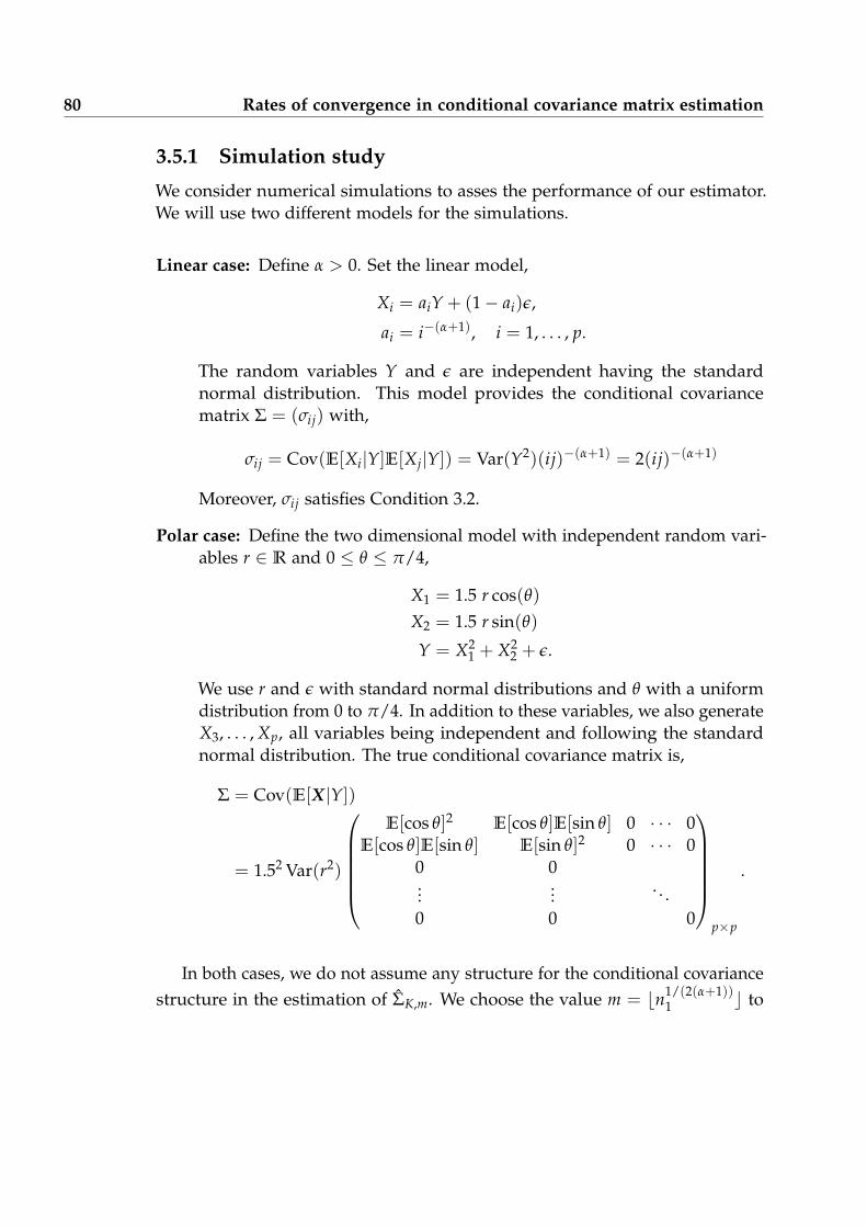
80 Rates of convergence in conditional covariance matrix estimation
3.5.1 Simulation study
We consider numerical simulations to asses the performance of our estimator.We will use two different models for the simulations.
Linear case: Define α > 0. Set the linear model,
Xi = aiY + (1− ai)ε,
ai = i−(α+1), i = 1, . . . , p.
The random variables Y and ε are independent having the standardnormal distribution. This model provides the conditional covariancematrix Σ = (σij) with,
σij = Cov(E[Xi|Y]E[Xj|Y]) = Var(Y2)(ij)−(α+1) = 2(ij)−(α+1)
Moreover, σij satisfies Condition 3.2.
Polar case: Define the two dimensional model with independent random vari-ables r ∈ R and 0 ≤ θ ≤ π/4,
X1 = 1.5 r cos(θ)X2 = 1.5 r sin(θ)
Y = X21 + X2
2 + ε.
We use r and ε with standard normal distributions and θ with a uniformdistribution from 0 to π/4. In addition to these variables, we also generateX3, . . . , Xp, all variables being independent and following the standardnormal distribution. The true conditional covariance matrix is,
Σ = Cov(E[X|Y])
= 1.52 Var(r2)
E[cos θ]2 E[cos θ]E[sin θ] 0 · · · 0
E[cos θ]E[sin θ] E[sin θ]2 0 · · · 00 0...
... . . .0 0 0
p×p
.
In both cases, we do not assume any structure for the conditional covariancestructure in the estimation of ΣK,m. We choose the value m = bn1/(2(α+1))
1 c to
3.6. Conclusion 81
regularize the estimated matrix ΣK. We set the threshold b in the first quantileof each estimation of f .
We consider a range of parameter values for n, p and α. The simulation usesvalues of α equals to 0.05, 0.1 and 0.5. Both p and n varying between 100 to600. To estimate the kernel functions gi and f we use the software R along thelibrary np ().
Table 3.1 reports the average error under the Frobenius norm over 100replications for the linear and polar case respectively. The mean error decreaseswith a rate equivalent to p/n as n increases due to the regularity of the model.In other words, in both cases fY and gi belong to a Hölder class with β ≥ 2.These results highlight the convergence of ΣK,m without any assumption in thedata structure.
3.5.2 Graphical representations
We next examine a simple application to the projection of data in a reducedspace. The models remains exactly the sames as before (linear and polar cases).In this section, we have generated 500 data points for each model over 200variables.
We compare the projected points calculated by our method against the clas-sical the sliced inverse regression method proposed by Li (1991a) implementedin the package dr.
The results in general are satisfactory. Figure 3.1 shows the data representa-tion in the linear model. In this case, both methods capture well most of themodel information. The polar case is presented in Figure 3.2. We observe howour method performs similar to the classic sliced inverse regression capturingthe data curvature for the first direction.
In Figure 3.3 and Figure 3.4, we observe that our method behaves better withrespect to the explained variance of the model. The nonparametric estimatorexplains around 60% of the variance with around 50 variables. In the meantime,the classic sliced inverse regression describes at most 40% of the variance withthe same number of variables. We have set in 0 all the negative eigenvalues,therefore the curves in the nonparametric cases remains constant at the end.
3.6 Conclusion
In this chapter we have investigated the rate of convergence for a nonparamet-rical estimator for the conditional covariance Cov(E[X|Y]). We have started

82 Rates of convergence in conditional covariance matrix estimation
α
p n 0.05 0.1 0.5
100 100 0.0090 0.0073 0.0049200 0.0054 0.0050 0.0031300 0.0042 0.0039 0.0024400 0.0040 0.0035 0.0021500 0.0037 0.0033 0.0019600 0.0034 0.0031 0.0019
200 100 0.0070 0.0063 0.0041200 0.0037 0.0036 0.0022300 0.0028 0.0026 0.0016400 0.0024 0.0022 0.0013500 0.0022 0.0020 0.0011600 0.0021 0.0018 0.0010
300 100 0.0066 0.0065 0.0040200 0.0034 0.0034 0.0019300 0.0024 0.0021 0.0014400 0.0020 0.0018 0.0010500 0.0017 0.0015 0.0009600 0.0016 0.0014 0.0008
400 100 0.0059 0.0055 0.0041200 0.0029 0.0028 0.0018300 0.0021 0.0019 0.0012400 0.0017 0.0016 0.0009500 0.0015 0.0013 0.0008600 0.0013 0.0012 0.0007
500 100 0.0071 0.0052 0.0060200 0.0028 0.0028 0.0016300 0.0020 0.0018 0.0012400 0.0016 0.0014 0.0008500 0.0013 0.0012 0.0007600 0.0012 0.0011 0.0006
600 100 0.0062 0.0057 0.0036200 0.0027 0.0026 0.0016300 0.0019 0.0017 0.0011400 0.0015 0.0014 0.0008500 0.0012 0.0011 0.0007600 0.0011 0.0010 0.0006
(a) Linear case.
α
p n 0.05 0.1 0.5
100 100 0.0513 0.0403 0.0336200 0.0178 0.0187 0.0155300 0.0139 0.0142 0.0116400 0.0118 0.0114 0.0104500 0.0110 0.0108 0.0098600 0.0106 0.0104 0.0096
200 100 0.0536 0.0508 0.0346200 0.0154 0.0161 0.0117300 0.0093 0.0097 0.0077400 0.0081 0.0077 0.0067500 0.0071 0.0070 0.0059600 0.0064 0.0063 0.0054
300 100 0.0594 0.0505 0.0251200 0.0145 0.0138 0.0103300 0.0094 0.0081 0.0075400 0.0068 0.0067 0.0051500 0.0057 0.0054 0.0045600 0.0050 0.0048 0.0042
400 100 0.0664 0.0411 0.0260200 0.0156 0.0118 0.0095300 0.0085 0.0080 0.0064400 0.0060 0.0058 0.0043500 0.0050 0.0048 0.0038600 0.0043 0.0042 0.0033
500 100 0.0377 0.0395 0.0350200 0.0129 0.0140 0.0092300 0.0076 0.0074 0.0054400 0.0060 0.0054 0.0041500 0.0048 0.0044 0.0034600 0.0040 0.0038 0.0029
600 100 0.0570 0.0430 0.0350200 0.0134 0.0132 0.0091300 0.0078 0.0071 0.0049400 0.0057 0.0052 0.0037500 0.0045 0.0042 0.0032600 0.0037 0.0034 0.0027
(b) Polar case.
Table 3.1: Average errors under the Frobenius norm of the nonparametricconditional covariance estimator over 100 replications.

3.6. Conclusion 83
−2 −1 0 1 2
−3
−2
−1
01
23
Classic SIR
X1
Y
−2 −1 0 1 2
−3
−2
−1
01
23
Kernel based SIR
X1
Y
−2 −1 0 1 2
−3
−2
−1
01
23
X2
Y
−2 −1 0 1 2
−3
−2
−1
01
23
X2
Y
Figure 3.1: Linear case: Real data against projected data. The black circlesrepresents the original data. The red crosses represent the projected points forthe linear model.
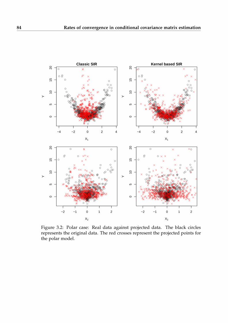
84 Rates of convergence in conditional covariance matrix estimation
−4 −2 0 2 4
05
1015
20
Classic SIR
X1
Y
−4 −2 0 2 40
510
1520
Kernel based SIR
X1
Y
−2 −1 0 1 2
05
1015
20
X2
Y
−2 −1 0 1 2
05
1015
20
X2
Y
Figure 3.2: Polar case: Real data against projected data. The black circlesrepresents the original data. The red crosses represent the projected points forthe polar model.
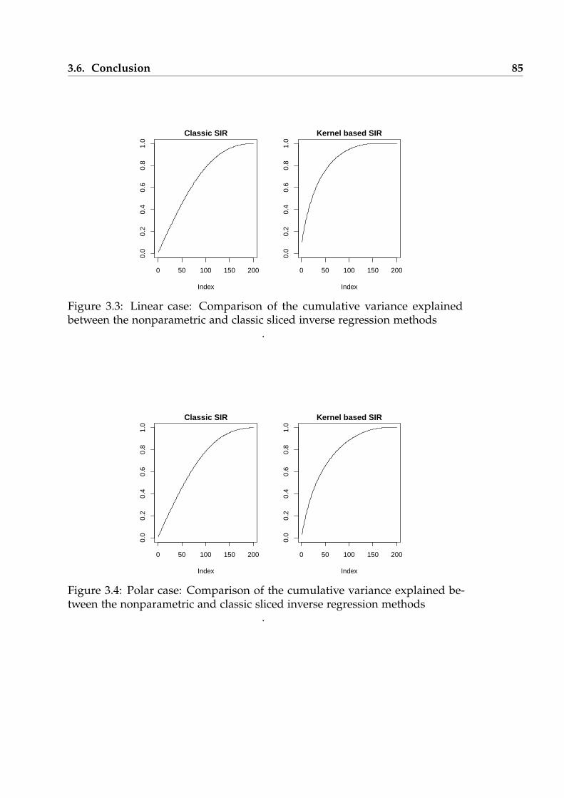
3.6. Conclusion 85
0 50 100 150 200
0.0
0.2
0.4
0.6
0.8
1.0
Index
Classic SIR
0 50 100 150 200
0.0
0.2
0.4
0.6
0.8
1.0
Index
Kernel based SIR
Figure 3.3: Linear case: Comparison of the cumulative variance explainedbetween the nonparametric and classic sliced inverse regression methods
.
0 50 100 150 200
0.0
0.2
0.4
0.6
0.8
1.0
Index
Classic SIR
0 50 100 150 200
0.0
0.2
0.4
0.6
0.8
1.0
Index
Kernel based SIR
Figure 3.4: Polar case: Comparison of the cumulative variance explained be-tween the nonparametric and classic sliced inverse regression methods
.

86 Rates of convergence in conditional covariance matrix estimation
studying the nonparametric behavior of each element of the matrix based inthe work of Zhu and Fang (1996). This approach, allow us to find rate ofconvergence depending on the value of β for the classical mean squared error.We have shown that if the model is regular enough, it is possible to achievethe parametric rate 1/n. Otherwise, we get a slower rate (log2(n)/n)2β/(β+2),depending on the regularity β of certain Hölder class.
As a natural extension, we studied the performance of mean squared riskof ΣK under the Frobenius norm. In order to keep the consistency and avoidissues due to the high-dimension data, it is necessary regularize the matrix ΣK.We used a regularized version of ΣK called ΣK,m, obtained by doing a Schurmultiplication between ΣK and a definite-positive matrix of weights. Thoseweights are 1 until some point away from the diagonal when they turn in 0.
This method could not ensure the positive definiteness of the estimate—butsince we proved that under some mild conditions, our estimator is consistentgiven either p/n → 0 or p(log2(n)/n)2β/(β+2) → 0, the estimator will be pos-itive definite with probability tending to 1. Other practical solution for thisissue is suggested by Cai et al. (2010). He proposes project ΣK to the space ofpositive-semidefinite matrices under the operator norm. In other words, firstdiagonalize ΣK and replace the negative eigenvalues by 0. The matrix obtainedis then semidefinite positive.
There are several alternatives norms to compute and matrix-based error,among them the operator norm. However, this approach would require theestimation of concentration inequalities for some specific matrices blocks of ΣKwhich is not suitable in our context. Nevertheless, the use of the operator normin the nonparametric estimation of Σ is worth to investigate.
3.7 Appendix
3.7.1 Technical lemmas
Lemma 3.3 (cf. Rao and Prakasa Rao (1983), Theorem 2.1.8). Suppose that K is akernel of order s = bβc and Assumption 3.1 is fulfilled. Then
supy| f (y)− f (y)| = O
(hβ +
log nn1/2h
).
The following lemma is a modified version of Theorem 2.37 of Pollard (1984).
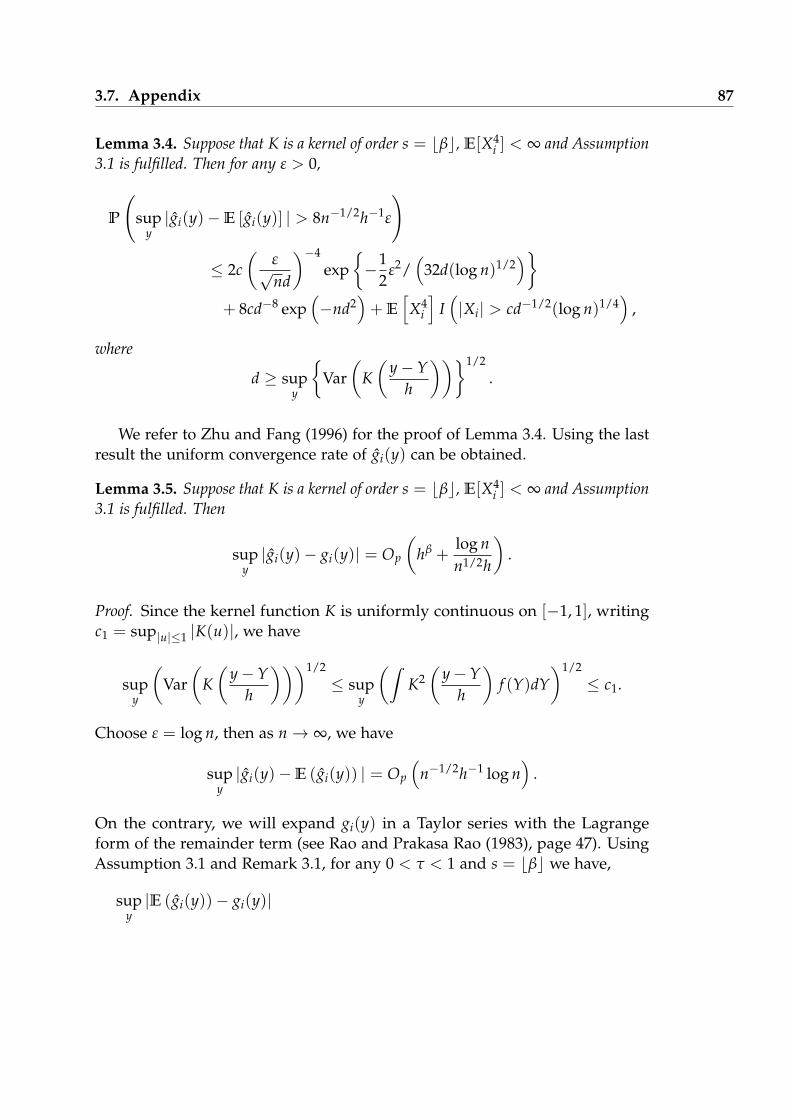
3.7. Appendix 87
Lemma 3.4. Suppose that K is a kernel of order s = bβc, E[X4i ] < ∞ and Assumption
3.1 is fulfilled. Then for any ε > 0,
P
(sup
y|gi(y)−E [gi(y)] | > 8n−1/2h−1ε
)
≤ 2c(
ε√nd
)−4
exp{−1
2ε2/
(32d(log n)1/2
)}+ 8cd−8 exp
(−nd2
)+ E
[X4
i
]I(|Xi| > cd−1/2(log n)1/4
),
where
d ≥ supy
{Var
(K(
y−Yh
))}1/2
.
We refer to Zhu and Fang (1996) for the proof of Lemma 3.4. Using the lastresult the uniform convergence rate of gi(y) can be obtained.
Lemma 3.5. Suppose that K is a kernel of order s = bβc, E[X4i ] < ∞ and Assumption
3.1 is fulfilled. Then
supy|gi(y)− gi(y)| = Op
(hβ +
log nn1/2h
).
Proof. Since the kernel function K is uniformly continuous on [−1, 1], writingc1 = sup|u|≤1 |K(u)|, we have
supy
(Var
(K(
y−Yh
)))1/2
≤ supy
(ˆK2(
y−Yh
)f (Y)dY
)1/2
≤ c1.
Choose ε = log n, then as n→ ∞, we have
supy|gi(y)−E (gi(y)) | = Op
(n−1/2h−1 log n
).
On the contrary, we will expand gi(y) in a Taylor series with the Lagrangeform of the remainder term (see Rao and Prakasa Rao (1983), page 47). UsingAssumption 3.1 and Remark 3.1, for any 0 < τ < 1 and s = bβc we have,
supy|E (gi(y))− gi(y)|
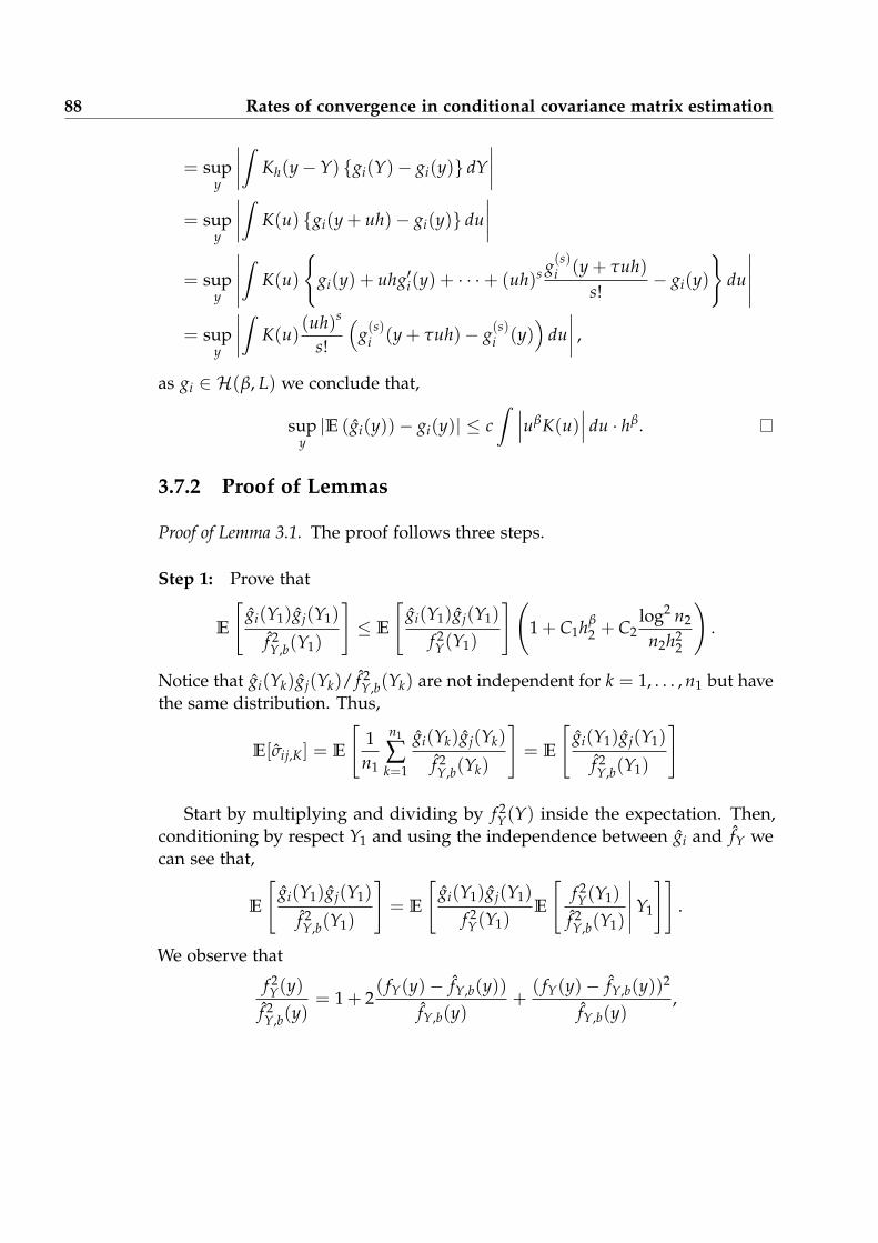
88 Rates of convergence in conditional covariance matrix estimation
= supy
∣∣∣∣ˆ Kh(y−Y) {gi(Y)− gi(y)} dY∣∣∣∣
= supy
∣∣∣∣ˆ K(u) {gi(y + uh)− gi(y)} du∣∣∣∣
= supy
∣∣∣∣∣ˆ
K(u)
{gi(y) + uhg′i(y) + · · ·+ (uh)s g(s)i (y + τuh)
s!− gi(y)
}du
∣∣∣∣∣= sup
y
∣∣∣∣ˆ K(u)(uh)s
s!
(g(s)i (y + τuh)− g(s)i (y)
)du∣∣∣∣ ,
as gi ∈ H(β, L) we conclude that,
supy|E (gi(y))− gi(y)| ≤ c
ˆ ∣∣∣uβK(u)∣∣∣ du · hβ.
3.7.2 Proof of Lemmas
Proof of Lemma 3.1. The proof follows three steps.
Step 1: Prove that
E
[gi(Y1)gj(Y1)
f 2Y,b(Y1)
]≤ E
[gi(Y1)gj(Y1)
f 2Y(Y1)
](1 + C1hβ
2 + C2log2 n2
n2h22
).
Notice that gi(Yk)gj(Yk)/ f 2Y,b(Yk) are not independent for k = 1, . . . , n1 but have
the same distribution. Thus,
E[σij,K] = E
[1n1
n1
∑k=1
gi(Yk)gj(Yk)
f 2Y,b(Yk)
]= E
[gi(Y1)gj(Y1)
f 2Y,b(Y1)
]
Start by multiplying and dividing by f 2Y(Y) inside the expectation. Then,
conditioning by respect Y1 and using the independence between gi and fY wecan see that,
E
[gi(Y1)gj(Y1)
f 2Y,b(Y1)
]= E
[gi(Y1)gj(Y1)
f 2Y(Y1)
E
[f 2Y(Y1)
f 2Y,b(Y1)
∣∣∣∣∣Y1
]].
We observe that
f 2Y(y)
f 2Y,b(y)
= 1 + 2( fY(y)− fY,b(y))
fY,b(y)+
( fY(y)− fY,b(y))2
fY,b(y),
3.7. Appendix 89
By Lemma 3.3 and Remark 3.2, equation (3.7.2) turns into
E
[gi(Y1)gj(Y1)
f 2Y,b(Y1)
]
≤ E
[gi(Y1)gj(Y1)
f 2Y(Y1)
]1 + C1nc1
(hβ
2 +log n2
n1/22 h2
)+ C2n2c1
(hβ
2 +log n2
n1/22 h2
)2
≤ E
[gi(Y1)gj(Y1)
f 2Y(Y1)
](1 + C1(n
c1−βc22 + n1/2−c1−c2
2 log n2)).
To simplify the notations, we will write simply n = n1 and h = h1 throughSteps 2 to 4
Step 2: Prove that,
E
[gi(Y1)gj(Y1)
f 2Y(Y1)
]≤ C1
n− 1E
(Xi2Xj2K2
h(Y1 −Y2)
f 2Y(Y1)
)
+ C2
(n− 2n− 1
)E
(Xi2Xj3Kh(Y1 −Y2)Kh(Y1 −Y3)
f 2Y(Y1)
).
Denote
B = E
[gi(Y1)gj(Y1)
f 2Y(Y1)
].
Again, conditioning with respect to Y1 and developing all the terms, we obtain,
B =1
(n− 1)2 E
[1
f 2Y(Y1)
E
[(n
∑k=2
XikKh(Y1 −Yk)
)(n
∑k=2
XjkKh(Y1 −Yl)
) ∣∣∣∣∣Y1
]]
=1
(n− 1)2 E
[1
f 2Y(Y1)
E
[n
∑k=2
XikXjkK2h(Y1 −Yk)
∣∣∣∣∣ Y1
]]
+1
(n− 1)2 E
1f 2Y(Y1)
E
n
∑k,r=2k 6=r
XikXjrKh(Y1 −Yk)Kh(Y1 −Yr)
∣∣∣∣∣ Y1
.
Therefore,
90 Rates of convergence in conditional covariance matrix estimation
E[σij,K] =C1
n− 1E
[Xi2Xj2K2
h(Y1 −Y2)
f 2Y(Y1)
]
+ C2
(n− 2n− 1
)E
[Xi2Xj3Kh(Y1 −Y2)Kh(Y1 −Y3)
f 2Y(Y1)
]≡ B1 + B2. (3.14)
Step 3: Prove that
B1 ≤Cnh
.
We start with
B1 =1
n− 1E
(Xi2Xj2K2
h(Y1 −Y2)
f 2Y(Y1)
)
=1
n− 1
ˆ1
f 2Y(y1)
xixjK2h(y1 − y2) f (xi, y2) f (xj, y2) fY(y1)dxidxjdy2dy1
=1
n− 1
ˆ1
fY(y1)xixjK2
h(y1 − y2) f (xi, y2) f (xj, y2)dxidxjdy2dy1
=1
(n− 1) h
ˆ1
fY(y1)xixjK2(u) f (xi, y1 + uh) f (xj, y1 + uh)dudxidxjdy1.
Remark that given am and bm, m = 1, 2 being real numbers such asam < bm, the integrals containing the coordinate (x, y) will be evaluatedin the cube [a1, b1]× [a2, b2].
Define the supremum norm of f as ‖ f ‖∞ = sup{ f (x, y) ∈ [a1, b1]× [a2, b2]}.Therefore,
B1 ≤‖ f ‖2
∞(n− 1) h
ˆ1
fY(y1)xixjK2(u)dudxidxjdy1,
which leads toB1 ≤
Cnh
.
Step 4: Show that|B2 − σij| ≤ Ch2β.
The second term of (3.14) can be bounded as follows
3.7. Appendix 91
B2 =
(n− 2n− 1
)E
(Xi2Xj3Kh(Y1 −Y2)Kh(Y1 −Y3)
f 2Y(Y1)
)
≤ˆ (ˆ
xiKh(y1 − y) f (x, y)dxidy)
(ˆxjKh(y1 − y) f (x, y)dxjdy
)1
fY(y1)dy1. (3.15)
By Assumption 3.1 with s = bβc and for 0 < τ < 1 we have,ˆKh(y1 − y) f (x, y)dy− f (x, y)
=
ˆK(u) f (x, uh + y)du− f (x, y)
=
ˆK(u)
{f (x, y) + uh f ′(x, y) + · · ·+ f (s)(x, y + τuh)
s!(uh)j
}du
=1s!
ˆK(u) (uh)s f (s)(x, y + τuh)du.
Adding K(u)(uh)s f (s)(x, y) to the last integral and the fact that f (x, ·) ∈ H(β, L)we can see that,ˆ
Kh(y1 − y) f (x, y)dy− f (x, y)
=1s!
ˆK(u) (uh)s
{f (s)(x, y + τuh)− f (s)(x, y)
}du
≤ 1s!
ˆK(u) (uh)s (τuh)β−s du
≤(
1s!
ˆ|uβK(u)|du
)τhβ = Chβ.
Plugging this into (3.15) leads to,
|B2 − σij| ≤∣∣∣∣∣ˆ {(ˆ
xi
(Chβ + f (xi, y)
)dxi
)(ˆxj
(Chβ + f (xj, y)
)dxj
)
−(ˆ
xi f (xi, y)dxi
)(ˆxj f (xj, y)dxj
)}1
fY(y)dy
∣∣∣∣∣≤ C2h2β
∣∣∣∣∣ˆ xixj
fY(y)dxidxjdy
∣∣∣∣∣
92 Rates of convergence in conditional covariance matrix estimation
+ Chβ
∣∣∣∣∣(ˆ
xiRi(y)dxidy +
ˆxjRj(y)dxjdy
) ∣∣∣∣∣≤ C1hβ + C2h2β
≤ C1hβ.
Step 5: Gathering the results from Steps 1 to 4, we get
Bias(σij,K) ≤(
C1hβ1 +
C2
n1h1
)(1 + C3(n
c1−βc22 + n1/2−c1−c2
2 log n2)).
Since h1 → 0 and n1h1 → ∞ as n1 → ∞, we obtain
Bias2(σij,K) ≤ C1h2β1 +
C2
n21h2
1.
Proof of Lemma 3.2. The proof will be done in several steps. Define
Ri,b(Y) =gi(Y)fY(Y)
,
V1(Y) =gi(Y)gj(Y)
f 2Y,b(Y)
= Ri,bRj,b,
V2(Y) =gi(Y)
f 2Y,b(Y)
(gj(Y)− gj(Y)
)=
Ri,b
fY(Y)(
gj(Y)− gj(Y))
,
V3(Y) =gj(Y)
f 2Y,b(Y)
(gi(Y)− gi(Y)) =Rj,b
fY(Y)(gi(Y)− gi(Y)) ,
V4(Y) =1
f 2Y,b(Y)
(gi(Y)− gi(Y))(
gj(Y)− gj(Y))
,
Jn(Y) = (V1(Y) + V2(Y) + V3(Y) + V4(Y))(2( fY(Y)− fY,b(Y))
fY,b(Y)+
( fY(Y)− fY,b(Y))2
f 2Y,b(Y)
).
It is clear that σij,K = n−11 ∑n1
k=1 V1(Yk) + V2(Yk) + V3(Yk) + V4(Yk) + Jn(Yk). IfC > 0, then the variance Var(σij,K) is bounded by
C
{Var
(1n1
n1
∑k=1
V1(Yk)
)+ Var
(1n1
n1
∑k=1
V2(Yk)
)+ Var
(1n1
n1
∑k=1
V3(Yk)
)
3.7. Appendix 93
+ Var
(1n1
n1
∑k=1
V4(Yk)
)+ Var
(1n1
n1
∑k=1
Jn(Yk)
)}.
We are going to bound every term separately.
Step 1: Prove that
Var
(1n1
n1
∑k=1
Jn(Yk)
)≤ C(n2c1−4βc2 + n2c1+2c2−1 log n).
We bound first the term
J1n =1n1
n1
∑k=1
V1(Yk)( fY(Yk)− fY,b(Yk))
fY,b(Yk).
Using Cauchy-Schwartz’s inequality, it is straightforward that
Var(J1n) ≤1n2
1E
( n1
∑k=1
gi(Yk)gj(Yk)
f 2Y,b
(fY(y)− fY,b(y)
fY,b(y)
))2
≤ 1n1
E
n1
∑k=1
(gi(Yk)gj(Yk)
f 2Y,b(Yk)
(fY(Yk)− fY,b(Yk)
fY,b(Yk)
))2 .
By Lemma 3.3 and Remark 3.2 we have
Var(J1n) ≤ CE
[1n1
n1
∑k=1
g2i (Yk)g2
j (Yk)
f 4Y,b(Yk)
]b−2(h2β + n−1/2h−1 log n)2
≤ C(n2c1−4βc2 + n2c1−1+2c2 log n),
where the second inequality is due to the law of large numbers for
1n1
n1
∑k=1
Ri,b(Yk)Rj,b(Yk).
To simplify the notation, we will write simply n = n1 and h = h1 throughSteps 2 to 4. Moreover we will denote Zk = (Xk, Yk) k = 1, . . . , n.
94 Rates of convergence in conditional covariance matrix estimation
Step 2. Prove that
Var(V1) ≤Cn
.
By independence of the Zk’s and given that gj, gl and fY are functions builtwith the second sample, it is clear that
Var
(1n
n
∑k=1
V1(Yk)
)= Var
(1n
n
∑k=1
Ri,b(Yk)Rj,b(Yk)
)
=1n
Var(
Ri,b(Y)Rj,b(Y))≤ C
n.
Step 3. Show that
Var (V2) + Var (V3) ≤C1
n+
C2
n2h.
First we get a bound of Var(V2). Note that,
V2 =1n
n
∑k=1
Ri,b(Yk)
fY(Yk)
(gj(Yk)− gj(Yk)
)=
1n(n− 1)
n
∑k=1
n
∑l=1l 6=k
Ri,b(Yk)
fY(Yk)
(XjlKh(Yk −Yl)− gj(Yk)
)
=1
n(n− 1)
n
∑k=1
n
∑l=1l 6=k
Ri,b(Yk)
fY(Yk)XjlKh(Yk −Yl)
− 1n(n− 1)
n
∑i=1
n
∑l=1l 6=k
Ri,b(Yk)Rj,b(Yk)
= V21 −V22.
Notice thatVar(V22) =
1n
Var(
Ri,b(Y)Rj,b(Y))=
Cn
.
The term V21 is indeed a one sample U-statistic of order two. Hence, if wedefine Zli = (Xli, Yk) and rewrite the expression, we get
V21 =1
n(n− 1)
n
∑k=1
n
∑l=1l 6= k
Ri,b(Yk)
fY(Yk)XjlKh(Yk −Yl)
3.7. Appendix 95
=12
(n2
)−1
∑(k,l)∈Cn
2
hi(Zik, Zil),
where Cn2 = {(k, l); 1 ≤ k < l ≤ n} and
hi(Zjk, Zjl) =Ri,b(Yk)
fY(Yk)XjkKh(Yk −Yl).
Employing the symmetric version of hi
hi(Zjk, Zjl) =12
(Ri,b(Yk)
fY(Yk)Xjl +
Ri,b(Yl)
fY(Yl)Xjk
)Kh(Yk −Yl),
it is possible (see Kowalski and Tu (2007) or Van der Vaart (2000)) to decomposeVar(V21) as
Var(V21) =
(n2
)−1{(21
)(n− 2
1
)Var(E(hi(Zj1, Zj2)|Zj1))
+
(22
)(n− 2
0
)Var(hi(Zj1, Zj2))
}.
Since fy(y) ≤ fY(y) we have,
E(hi(Zj1, Zj2)|Zj1)
=12
ˆKh(Y1 − y)
(xjRi,b(Y1)
fY(Y1)+
Xj1Ri(y)fY(y)
)f (xj, y)dxjdy
=Ri,b(Y1)
2 fY(Y1)
ˆKh(Y1 − y)Rj(y) fY(y)dy
+12
Xj1
ˆKh(Y1 − y)
Ri,b fY(y)fY(y)
dy
≤ 12
Ri(Y1)Rj(Y1) +12
Xj1Ri(Y1)
+Ri(Y1)
2 fY(Y1)
ˆKh(Y1 − y){Rj(y) fY(y)− Rj(Y1) fY(Y1)}dy
+12
Xj1
ˆKh(Y1 − y) {Ri(y)− Ri(Y1)} dy
≤ 12
Ri(Y1)Rj(Y1) +12
Xj1Ri(Y1) + J1(Zj1) + J2(Zj1).

96 Rates of convergence in conditional covariance matrix estimation
Using Assumption 3.1 and applying the same arguments as in the proof ofLemma 3.4, we can conclude that
Var(J1(Zj1)) ≤ E[(J1(Zj1))2]
≤ Ch2β
ˆ (Ri(y)fY(y)
)2(ˆ|usK(u)du|
)2
fY(y)dy
≤ Ch2βE[R2i (Y1)] ≤ Ch2β.
Moreover, as f ∈ H(β, L) and 0 < η < fY(y), we have
Var(J2(Zj1)) ≤ E[(J2(Zj1))2]
≤ 14
E
[X2
j1
(ˆK(u) (Ri(Y1 + uh)− Ri(Y1)du) du
)2]
≤ Ch2β.
Therefore,
Var(E(hi(Zj1, Zj2)|Zj1)) ≤ Var(
12
R2(Y1) +12
Xl1R(Y1)
)+ C1h2β.
By similar calculations we bound,
Var(hi(Zj1, Zj2)) ≤C2
h.
Using the same procedure we can bound Var(V3). We conclude that,
Var(V2) + Var(V3) ≤2
n(n− 1)
{(n− 2)
(C1 + C2h2β+
)+
C4
h
}≤ C1h2β +
C2
n2h.
Step 4. Show that
Var(V4) ≤ C(h4β + n−2h−4 log4 n).
Using Lemma 3.4 we obtain
Var (V4) ≤ E[V24 ]

3.7. Appendix 97
=1n2 E
( n
∑k=1
(gi(Yk)− gi(Yk))(
gj(Yk)− gj(Yk))
f 2Y(Yk)
)2
≤ Cn2
n2 (hβ + n−1/2h−1 log n)4
≤ C(hβ + n−1/2h−1 log n)4
≤ C(h4β + n−2h−4 log4 n).
Final bound Gathering all previous results, we have
Var(σij,K
)≤ C1h2β +
C2 log4 nn2h4 .

Chapter 4
Nonparametric estimator of Sobolindices
4.1 Introduction
In the areas of chemistry, biology, psychology or finance, the process of imple-menting some policy or taking some decision is often supported by complexmodels. The researcher has to process, analyze and interpret those systemswith numerous variables, high interactions and complexity. Two examples ofcomplex models are the following:
• One bank could buy some financial contract (e.g., European option) in-dexed to some rate of interest. This rate is unknown and depends oncomplex factors: market dynamics, inflation or political policies (see Hull(2011)). If the bank wants to sell the option, they face the risk associatedwith the interest rate movements. The goal, in general, is to avoid the riskexposure by holding this product and make the most profit with it.
• The Michaelis-Menten kinetics (Cornish-Bowden (2013)) models a sat-urable enzymatic degradation of a substance. The model is highly com-plex because it needs several experiments to estimate their parameters.In general, the scientists search to approximate stably the time of thereaction equilibrium. This process models the oxidation of glucose, whichproduces water, carbon dioxide and energy for instance.
99
100 Nonparametric estimator of Sobol indices
To handle those complexities, it is necessary identify the most importantvariables in the model. In the first example, the risk manager has to take adecision based in some financial model. Given the inherent complexity, heneeds to select the most relevant features on the model of rates. With the newset of relevant variables, he will gain insight on the model and it is possible takea better decision. Also, as the Michaelis-Menten kinetics, the model has to runstably to find the correct equilibrium. In other words, if the model suffer ofsmall alterations in the input, those should not produce large variations on theoutput. In any case, the analyst has to validate, check and correct the model ifit is necessary.
We assume a set of inputs variables X = (X1, . . . , Xp) ∈ Rp producing anoutput Y ∈ R related by the model
Y = m(X1, . . . , Xp). (4.1)
The function m is, generally, an unknown and complex function. However, acomputer code can gauge it in some cases (e.g., Oakley and O’Hagan (2004)).When the running time for the evaluation of such complex function are impor-tant, one could replace the original model by a meta-model (see Box and Draper(1987)).
The literature present techniques to rank the influences of the inputs (X1, . . . , Xp)in the model (4.1). Some of them are, for example, the screening method (Cullenand Frey (1999) Campolongo et al. (2011)), the automatic differentiation (Rall(1980), Carmichael et al. (1997)), the regression analysis (Draper and Smith(1981), Devore and Peck (1996)) or the response surface method (Myers et al.(2009), Goos (2002)).
Alternatively, Sobol’ (1993), inspired by a ANOVA (or Hoeffding) decom-position, split down the variance of the model in partial variances generatedby the conditionals expectations of Y giving each input Xi for i = 1, . . . , p.These partial variances represent the uncertainty created by each input or itsinteractions. Dividing each partial variance by the model total variance, weobtain a normalized index of importance. Specifically, we call the first-orderSobol indices to the quantities,
Si =Var(E[Y|Xi])
Var(Y)for i = 1, . . . , p.
Notice that E[Y|Xi] is the best approximation of Y given the information ofXi. Thus, if the variance of E[Y|Xi] is large, it means a large influence of Xi into
4.1. Introduction 101
Y. These indices are a widely used in theoretical and applied techniques andidentify the most relevant and sensible inputs on the model. We can constructindices that measure the interactions between variables or the total effect ofcertain input in the whole model. We refer the reader to Saltelli et al. (2000) forthe exact computation of higher-order Sobol indices.
The principle endeavor with the Sobol indices relays in its computation.Some methods propose the use of multiple samples (of the order of hundredsor thousands) for the evaluation of the model outputs. From applied problemsin engineering, biology, oceanography and others; the scientists have developedMonte-Carlo or quasi Monte-Carlo methods. For instance, the Fourier amplitudesensitivity test (FAST) or the Sobol pick-freeze (SPF). Cukier et al. (1973, 1978)created the FAST method which transforms the partial variances in Fourierexpansions. This method allows the aggregated and simple estimation of Sobolindices in an escalated way. The SPF scheme regresses the model output againsta pick-frozen replication. The principle is to create a replication holding theinterest variable (frozen variable) and resampling the other variables (pickedvariables). We refer to the reader to Sobol’ (1993, 2001) and Janon et al. (2013).Other methods include to Ishigami and Homma (1990) which improved theclassic Monte-Carlo procedure by resampling the inputs and reducing the wholeprocess to only one Monte-Carlo loop. Moreover, Saltelli (2002) proposed analgorithm to estimate higher-order indices with the minimum computationeffort.
The Monte-Carlo methods suffer of the high-computational stress in itsimplementation. For example, the FAST method requires estimate a set ofsuitable transformation functions and integer angular frequencies for eachvariable. The SPF scheme creates a new copy of the variable in each iteration.For complex and high-dimensional models, those techniques could be expensivein computational time.
The aim of this chapter propose an alternative way to compute the Sobolindices. In particular, we will take the ideas of Zhu and Fang (1996) and we shallapply a nonparametric Nadaraya-Watson to estimate the value Si for i = 1, . . . , p.With this estimator, we avoid the stochastic techniques and we use the structureof the data to fit the nonparametric model. We consider only the indices withsimple interaction between one variable with respect the output. We leaveout the sensitivity indices with interactions for a further study. Furthermore,we will show that if the joint distribution of (Xi, Y) is twice differentiable, thenonparametric estimator of Si, has a parametric rate of convergence. Otherwise,
102 Nonparametric estimator of Sobol indices
we will get a nonparametric rate of convergence depending on the regularity ofthe density.
In Section 4.2 we will propose the nonparametric estimator for the first-orderSobol indices. All the hypotheses and assumptions are gathered in Section4.3. We display the main result of this chapter in Section 4.4. We illustrate ourmethodology with some numerical examples in Section 4.5. Finally, in Section4.6, we discuss the results and expose some conclusions.
4.2 Methodology
In our context we suppose that X>k = (X1k, . . . , Xpk) and Yk, k = 1, . . . , n areindependent and identically distributed observations from the random vectorX> = (X1, . . . , Xp) and Y respectively. We denote by f (xi, y) the joint density ofthe couple (Xi, Y). Let fi(xi) =
´Rp f (xi, y)dy be the marginal density function
with respect to Xi for i = 1, . . . , p.
Recall the definition of Sobol indices presented in the introduction,
Si =Var(E[Y|Xi])
Var(Y)=
E[E[Y|Xi]]2 −E[Y]2
Var(Y)for i = 1, . . . , p. (4.2)
We have expanded the variance of the numerator to simplify the presentation.Notice that we can estimate the terms E[Y] and Var(Y) in equation (4.2) by theirempirical counterparts
Y =1n
n
∑k=1
Yk (4.3)
and
σY =1n
n
∑k=1
(Yk −Y)2 (4.4)
respectively.
Conversely, the estimation of the term E[E[Y|Xi]2] requires more effort. For
any i = 1, . . . , p we introduce the following notation,
Vi = E[E[Y|Xi]2] =
ˆ (´y f (xi, y) dy
fi(xi)
)2
fi(xi) dxi
4.2. Methodology 103
=
ˆ (gi(xi)
fi(xi)
)2
fi(xi) dxi,
where
gi(xi) =
ˆy f (xi, y) dy.
We will use a slightly modified version of the nonparametric estimator de-veloped in Loubes et al. (2013). This paper estimates the conditional expectationcovariance for a reduction dimension problem. Taking the same methodologyapplied to our case, define n1 < n and n2 = n− n2. For the sake of simplicitywe use n1 = n2 = n/2. Let h1 and h2 be two bandwidths depending on n1 andn2 respectively.
We will estimate the functions gi(x) and fi(x) respectively by their nonpara-metric estimators,
gi(x) =1
(n1 − 1)h1
n1
∑l=1l 6=k
YlK(
x− Xilh1
), (4.5)
fi(x) =1
n2h2
n2
∑l=1
K(
x− Xilh2
). (4.6)
Also, to avoid small values in the V’s estimation due to small values in thedenominator, let b > 0 a sequence of values satisfying
fi,b(x) = max{ fi(x), b}.
The nonparametric estimator for Vi is,
Vi =1n1
n1
∑k=1
(gi(Xik)
fi,b(Xik)
)2
. (4.7)
Therefore, gathering the estimators (4.3) and (4.7), we define the nonpara-metric estimator for Si as
Si =Vi −Y2
σY. (4.8)
The estimator (4.8) provides a direct way to estimate the first-order Sobolindex Si. We want to control the square risk over some regular class of functions
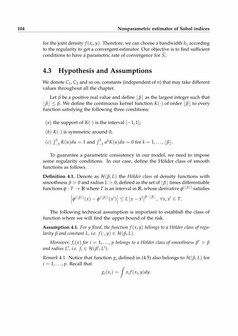
104 Nonparametric estimator of Sobol indices
for the joint density f (xi, y). Therefore, we can choose a bandwidth h1 accordingto the regularity to get a convergent estimator. Our objective is to find sufficientconditions to have a parametric rate of convergence for Si.
4.3 Hypothesis and Assumptions
We denote C1, C2 and so on, constants (independent of n) that may take differentvalues throughout all the chapter.
Let β be a positive real value and define bβc as the largest integer such thatbβc ≤ β. We define the continuous kernel function K(·) of order bβc to everyfunction satisfying the following three conditions:
(a) the support of K(·) is the interval [−1, 1];
(b) K(·) is symmetric around 0;
(c)´ 1−1 K(u)du = 1 and
´ 1−1 ukK(u)du = 0 for k = 1, . . . , bβc.
To guarantee a parametric consistency in our model, we need to imposesome regularity conditions. In our case, define the Hölder class of smoothfunctions as follows.
Definition 4.1. Denote as H(β, L) the Hölder class of density functions withsmoothness β > 0 and radius L > 0, defined as the set of bβc times differentiablefunctions φ : T → R where T is an interval in R, whose derivative φ(bβc) satisfies∣∣∣φ(bβc)(x)− φ(bβc)(x′)
∣∣∣ ≤ L∣∣x− x′
∣∣β−bβc , ∀x, x′ ∈ T.
The following technical assumption is important to establish the class offunction where we will find the upper bound of the risk.
Assumption 4.1. For y fixed, the function f (x, y) belongs to a Hölder class of regu-larity β and constant L, i.e. f (·, y) ∈ H(β, L).
Moreover, fi(x) for i = 1, . . . , p belongs to a Hölder class of smoothness β′ > β
and radius L′, i.e. fi ∈ H(β′, L′).
Remark 4.1. Notice that function gi defined in (4.5) also belongs to H(β, L) fori = 1, . . . , p. Recall that
gi(xi) =
ˆxi f (xi, y)dy.

4.4. Main result 105
Let y ∈ R fixed. If f (·, y) ∈ H(β, L) then by a direct calculation we can proveour assertion.
Denote as F = Fβ(L) the class of functions that fulfill Assumption 4.1. Inthe next section, we shall found the rates of convergence for σij depending onthe parameter β.
Remark 4.2. To control the term fX,b in the denominator on equation (4.7),we need to fix h2 and b—both sequences converging to zero—to ensure theconvergence of Vi. As n → ∞, set h2 ∼ n−c1 and b ∼ n−c2 with the positivesnumber c1 and c2 satisfying that c1/β < c2 < 1/2− c1, and the notation “∼”means that two quantities have the same convergence order.
4.4 Main result
The following theorem emphasizes the performance of our estimator.
Theorem 4.1. Assume that E |Xi|4 < ∞, i = 1, . . . , p. The upper bound risk of theestimator Si defined in (4.8) over the functional class F satisfies:
• if β ≥ 2 and choosing h1 ≈ n−1/41 then
supF
E[(Si − Si)2] ≤ C
n1. (4.9)
• if β < 2 and choosing h1 ≈ n−1/(β+2)1 then,
supF
E[(Si − Si)2] ≤ C
(log2(n1)
n1
)2β/(β+2)
. (4.10)
The proof of the Theorem 4.1 will be postponed to the Appendix 4.7.
Theorem 4.1 presents an elbow effect on the rates of convergences. This isa typical behavior in linked to studies on functional estimation, for instanceBaraud et al. (2003) or Laurent (2005). The regularity of the joint density functionf defines the rate of convergence for the mean squared risk of Si. It means, wecan get a parametric rate n−1
1 paying a price on the regularity of β ≥ 2. Whenβ < 2, the rate turn into a nonparametric one which depends on the parameterβ.
106 Nonparametric estimator of Sobol indices
In the regular case, when β ≥ 2, we avoid any adaptability problem withrespect to the choose of the bandwidth h1. We can ensure a parametric rateof convergence for Si taking a bandwidth of hi = n−1/4. In other case, it isnecessary to be aware of the regularity of our model to choose the bandwidth.
4.5 Numerical illustrations
In this section, we illustrate the asymptotic results with some tests function forsensitivity analysis. The reader can find an abundant list of well-known testfunctions in the Section 2.9 of Saltelli et al. (2000).
In all the simulations we will took n equal to 1000, 2000, 5000 and 10000 foreach case. We repeated the experiment 100 times selecting a different samplein each iteration. The inputs are gaussian random variables with mean 0 andvariance specified in each configuration. The horizontal full lines in the graphicsrepresent the theoretical Sobol index for each variable. We used the packagemoments (Komsta and Novomestky (2011)) using a sample of 106 observationsto estimate those theoretical values. Also, we used the package np (Hayfieldand Racine (2008)) for the kernel estimators.
4.5.1 Ishigami model
The Ishigami function (cf. Ishigami and Homma (1990)) will generate our firstsimulation study. We use the following configuration,
Y = sin X1 + 7 sin2 X2 + 0.1 X43 sin X1 (4.11)
where Xi ∼ N (0, 1.252) for i = 1, 2, 3.
The Ishigami function is a popular model in sensitivity analysis becausepresents a strong nonlinearity and nonmonotonicity with interactions in X3.For a further explanation of this function, we refer the reader to Sobol’ andLevitan (1999). We will present only the first-order Sobol indices of the Ishigamifunction in this work. We choose a bandwidth of h = n−1/4 for each sample.
Figure 4.1 summarizes the simulation results. Our method has estimatedcorrectly the Sobol indices for each input. The bias is inherent in the modeldue to the choose of our bandwidth. We appreciate strongly this effect forthe inputs X2 and X3. The bandwidth h = n−1/4 is sub-optimal. We expectedit due to we have established only an upper bound for the kernel estimator.Even so, the variance is well controlled and decrease as we raise the number
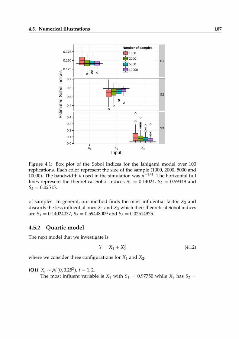
4.5. Numerical illustrations 107
●●●● ●
●
●
●●●
●
●
●
●●
●●
●
●
●●●●●
●●
●
●
●●
●
●
●
0.125
0.150
0.175
0.4
0.5
0.6
0.7
0.0
0.1
0.2
0.3
0.4
S1
S2
S3
X1 X2 X3
Input
Est
imat
ed S
obol
indi
ces
Number of samples
1000
2000
5000
10000
Figure 4.1: Box plot of the Sobol indices for the Ishigami model over 100replications. Each color represent the size of the sample (1000, 2000, 5000 and10000). The bandwidth h used in the simulation was n−1/4. The horizontal fulllines represent the theoretical Sobol indices S1 = 0.14024, S2 = 0.59448 andS3 = 0.02515.
of samples. In general, our method finds the most influential factor X2 anddiscards the less influential ones X1 and X3 which their theoretical Sobol indicesare S1 = 0.14024037, S2 = 0.59448009 and S3 = 0.02514975.
4.5.2 Quartic model
The next model that we investigate is
Y = X1 + X42 (4.12)
where we consider three configurations for X1 and X2:
(Q1) Xi ∼ N (0, 0.252), i = 1, 2.The most influent variable is X1 with S1 = 0.97750 while X2 has S2 =

108 Nonparametric estimator of Sobol indices
0.022510.
(Q2) Xi ∼ N (0, 0.52), i = 1, 2.Both variables have comparable influence with S1 = 0.39710 and S2 =0.60150.
(Q3) Xi ∼ N (0, 1), i = 1, 2.The variable X2 has the greater Sobol index S2 = 0.98977 against S1 =0.01031 for X1.
We have simulated the quartic model with two settings for the bandwidthvalues: (a) selected by the cross-validation method implemented in the packagenp, and (b) fixed to h = 1/16 n−1/4 according to Theorem 4.1. For the theoreticalbandwidths we used the values 0.01111, 0.00935, 0.00743 and 0.00625 for thesamples 1000, 2000, 5000 and 10000 respectively. The Table 4.1 presents theaverage bandwidths estimated by cross-validation for each Sobol index andeach configuration.
Q1 Q2 Q3
S1 S2 S1 S2 S1 S2
1000 0.02260 0.09704 0.11040 0.06954 0.63539 0.068772000 0.02074 0.07039 0.09777 0.05354 0.47266 0.139965000 0.01741 0.05959 0.08991 0.03869 0.41863 0.03519
10000 0.01524 0.05323 0.08064 0.04176 0.38029 0.04588
Table 4.1: Average bandwidths estimated by the built-in cross-validation methodof the package np for the Sobol indices S1 and S2 with the configurations Q1,Q2 and Q3.
Figures 4.2, 4.3 and 4.4 represent the box plots of the Sobol indices for theconfigurations Q1, Q2 and Q3 respectively. First, notice that the simulationstaking the bandwidth chosen by the np cross-validation estimator performedpoorly. In particular, they present a bias consistently in all the configurations.This is due that the package np optimizes its procedure for nonparametricfunctional or regression estimation. It ignores any particular structure of theconditional variance Var(E[Y|Xi]). Still, using these values the method canapproximate the theoretical values and control the variance as the sampleincreases.

4.5. Numerical illustrations 109
●●
●●●●
●
●
●
●
●●●
●
●
●●●
●●
●
●●
0.92
0.94
0.96
0.98
0.00
0.02
0.04
0.06
S1
S2
X1 X2
Input
Est
imat
ed S
obol
indi
ces
Number of samples
1000
2000
5000
10000
(a) Bandwidth chosen by cross-validation using the package np.
●
●
●
●
●
●
●
●●
●●●●
●●
●●●●
●
●
●
●
0.94
0.96
0.98
0.03
0.06
0.09
S1
S2
X1 X2
Input
Est
imat
ed S
obol
indi
ces
Number of samples
1000
2000
5000
10000
(b) Bandwidth set to 1/16 n−1/4.
Figure 4.2: Box plot of the Sobol indices for the analytical model Y = X1 + X42
over 100 replications for the configuration (Q1). Each color represent the size ofthe sample (1000, 2000, 5000 and 10000). The horizontal full lines represent thetheoretical Sobol indices S1 = 0.97750 and S2 = 0.02251.
110 Nonparametric estimator of Sobol indices
●
●
●
●
●
●
●●
●
●
●
●
●●
●
●
0.2
0.3
0.4
0.5
0.6
0.7
0.3
0.4
0.5
0.6
0.7
0.8
S1
S2
X1 X2
Input
Est
imat
ed S
obol
indi
ces
Number of samples
1000
2000
5000
10000
(a) Bandwidth chosen by cross-validation using the package np.
●
●
●
●
●
●
●
●
●●
●
●
●
●
●●
0.1
0.2
0.3
0.4
0.5
0.6
0.4
0.5
0.6
0.7
0.8
0.9
S1
S2
X1 X2
Input
Est
imat
ed S
obol
indi
ces
Number of samples
1000
2000
5000
10000
(b) Bandwidth set to 1/16 n−1/4.
Figure 4.3: Box plot of the Sobol indices for the analytical model Y = X1 + X42
over 100 replications for the configuration (Q2). Each color represent the size ofthe sample (1000, 2000, 5000 and 10000). The horizontal full lines represent thetheoretical Sobol indices S1 = 0.39710 and S2 = 0.60150.
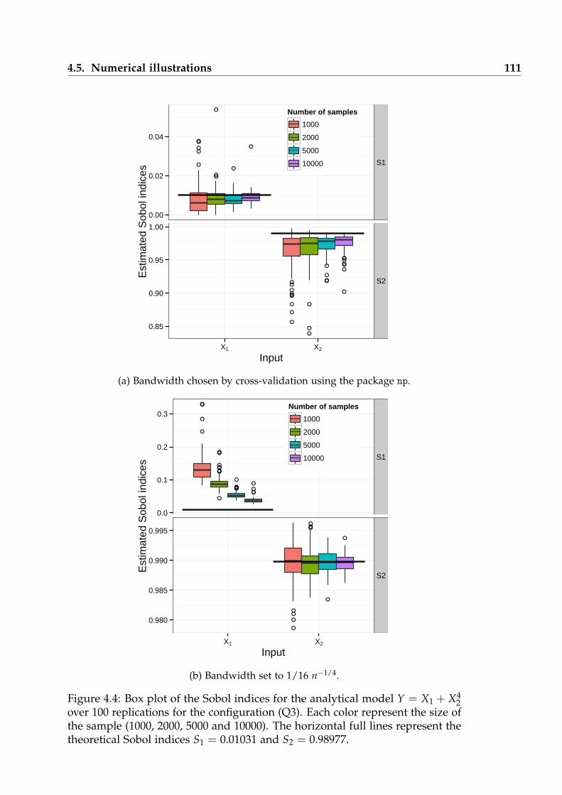
4.5. Numerical illustrations 111
●
●
●
●
●
●●
●
●
●
●
●
●
●
●
●●●
●
●●
●
●
●
●
●
●
●●
●●●
●
0.00
0.02
0.04
0.85
0.90
0.95
1.00
S1
S2
X1 X2
Input
Est
imat
ed S
obol
indi
ces
Number of samples
1000
2000
5000
10000
(a) Bandwidth chosen by cross-validation using the package np.
●
●
●
●
●
●
●●
●●
●●●
●●●●
●
●●●
●
●
●●
●
●●●
●
●
0.0
0.1
0.2
0.3
0.980
0.985
0.990
0.995
S1
S2
X1 X2
Input
Est
imat
ed S
obol
indi
ces
Number of samples
1000
2000
5000
10000
(b) Bandwidth set to 1/16 n−1/4.
Figure 4.4: Box plot of the Sobol indices for the analytical model Y = X1 + X42
over 100 replications for the configuration (Q3). Each color represent the size ofthe sample (1000, 2000, 5000 and 10000). The horizontal full lines represent thetheoretical Sobol indices S1 = 0.01031 and S2 = 0.98977.
112 Nonparametric estimator of Sobol indices
Using the theoretical bandwidth 1/16 n−1/4, we improve our results. Themethod reduces both the bias and the variance in every case as we raise thenumber of observations. Compared with the cross-validation choice, we see howthe averages of our method stay close of the theoretical Sobol indices. Figures4.2b and 4.4b present strong biases for the sample of 1000, but they shrink as weincrement to 10000 observations. Independently of the choice of the bandwidth,our methodology has identified the most relevant input for each case.
4.6 Conclusion
In this work, we focused our attention in the estimation of first-order Sobolindices. These indices measure the impact of the inputs to the output in generalmodels. We presented a nonparametric estimator based in the work proposedpreviously by Loubes et al. (2013).
This procedure provides a direct way to estimate the Sobol indices with-out run any expensive Monte-Carlo simulation. In real sensitivity analysisapplications, this advantage could give fast answers and create better models.
We have shown that the mean square risk of our estimator attains a para-metric rate of convergence, if the regularity of the model is smooth enough.In other case, we can only ensure a slower rate depending on the regularityof the model. This is interesting from the theoretical point of view becausesets parametric properties to a nonparametric object. Moreover, it is possibleto extend this technique to higher-order indices. The idea is use multivariatekernels in equations (4.5) and (4.6). We will explore higher-order indices in afurther work. Moreover, we have to improve the rates of convergence finding alower bound to proof the optimality.
The numerical simulations shown that our model identify correctly theSobol indices in each case presented. The configurations used were set withgaussian inputs. We compared the bandwidth proposed in Theorem 4.1 againstthe estimated by the np package. The results for the choice of our bandwidthperformed better than the cross-validation one. This is because the np is notoptimized for conditional variance regression. In general, it is hard understandthe regularity of the joint densities. However, in a future work, we could developa cross-validation scheme suited for this framework.
We have to test further our estimator, but the first results are promising. Also,it would be interesting apply this algorithm to real data and test its capabilities.

4.7. Appendix 113
4.7 Appendix
4.7.1 Proof of Theorem 4.1
Proof. Notice that
E[(Si − Si)2] = E
( Vi −Y2
σY− Vi −E[Y]
Var(Y)
)2
≤ E
(Y2
σY− E[Y]
Var(Y)
)2+ E
( Vi
σY− Vi
Var(Y)
)2 . (4.13)
The first term in equation (4.13) the it is easy to bound by n−1 applying thedelta-method. Now adding and subtracting Vi/σY in the right term, we candecompose it in the following way,
E
( Vi
σY− Vi
Var(Y)
)2 = E
( Vi
σY
(σY − σY)
σY
)2+ E
( Vi −Vi
σY
)2 (4.14)
Given that the kernel function K and the value E[X4i ] are bounded, we
can apply the Cauchy-Schwarz inequality to left term in equation (4.14). Wecan establish that there exist a real number M > 0 such as E[(Vi/σY)
4] ≤ M.Moreover, applying once again the delta-method, we can control the value
E
[(σY − σY
σY
)2]≤ 1
n.
Finally, for the termE[(Vi −Vi)
2]
in equation (4.14) we will apply directly the Theorem 1 of Loubes et al. (2013).We use the same reasoning in that proof: If β ≥ 2 and choosing h1 = n−1/4
1 weobtain
supF
E[(Si − Si)2] ≤ C
n1.
114 Nonparametric estimator of Sobol indices
Otherwise, taking h1 = n−1/(β+2)1 the upper bound turns into
supF
E[(Si − Si)2] ≤ C
(log2(n1)
n1
)2β/(β+2)
.
This proves the theorem.

Conclusions and perspectives
In this thesis we studied the estimation of the conditional covariance matrix fortwo main problems: reduction dimension and sensibility analysis. We assumed,generally, a nonlinear regression model with X ∈ Rp the independent variableand Y ∈ R the dependent variable. Also we assume that p is bigger than thenumber of observations available in the experiment.
In the first part we concentrate our efforts finding an estimator for theconditional covariance matrix Σ = Cov(E[X|Y]). We introduced this matrix asa collateral result for the sliced inverse regression method. In short, once wehave the spectral space of Σ, we can identify a reduced and more informativeset of coordinates. This new coordinates will serve us to explore further thedata, applying other technique like classification, regression, etc.
Then we moved our interest to study the value Var(E[Y|X]) for X ∈ R andY ∈ R. This quantity is directly linked with the estimation of Sobol indices forsensitivity analysis. The Sobol indices measure the impact of the inputs into theoutput inside a model.
We proposed different nonparametric methods to tackle those issues. Wewill summarize briefly the results that we obtained and give some perspectivesabout the ongoing work.
The Taylor estimator
In Chapter 2 we presented an estimator based on the Taylor decomposition of ageneral functional T associated with the coordinate-wise conditional covariance.We used a general basis of orthonormal functions to project the functional T
115
116 Conclusions and perspectives
onto its span. We found that the variance of the Taylor estimator depends onlyon the linear part of its development. This characteristic, causes that the Taylorestimator is efficient from the Cramér-Rao point of view. In other words, itattains the minimum variance among the other estimators. Finally we found theasymptotic variance for the whole matrix estimator and proved its asymptoticnormality.
There are still several topics about this subject to explore. It would beinteresting study the behavior of our estimator using particular sets of functionalbasis like wavelets, splines or polynomial functions (Legendre, Laguerre andso on). We explained briefly this topic with a general wavelet basis, but theidea is to expand it to a wider set of basis and find some simplifications in theestimator. This steps will allow us to implement it easier in future applications.
Another point worth to investigate the Cramér-Rao efficiency of the wholematrix estimator. We can provide the result with a half-vectorized version ofthe conditional covariance matrix.
The kernel-based estimator
We proposed a nonparametric estimator for the conditional covariance in Chap-ter 3 and used the same idea for to find an estimator for the first-order Sobolindices in Chapter 4. We proved that under some mild conditions, the element-wise estimator’s mean squared error achieves a parametric rate of convergence.In the case of Chapter 3, we observed a similar behavior for the full matrixestimator under the Frobenius norm. We performed simulations with some testcases.
One of the key point in the methodology was split the sample in two equalparts to get the independence between the numerator and denominator. Oneimprovement to our methodology is to find some way to split the sampleadaptatively preserving the result. Also, we limited our work to the Frobeniusnorm, but it would be interesting find rates of convergence under other normslike the operator-norm.
One of the most encouraging ideas ongoing in both estimators are theminimax and adaptive rates of convergence. There are plenty of literature aboutminimax lower bound for the sample covariance, for instance Cai et al. (2010).Find a rate of this kind, would prove that our estimators are optimal under someregularity conditions. Moreover, given that our rate depends on the regularitylevel β, search adaptive rates of convergence will produce attractive results.

Conclusions and perspectives 117
Real case simulations
We made some simulations in Chapters 3 and 4 with testing models for theconditional covariance and variance respectively. We used the nonparametricestimators in examples of reduction dimension and sensitivity analysis. Forthe Taylor estimator, proposed in Chapter 2, we have already an incompleteimplementation which needs to be improved for real simulations. Therefore, wehave two main objectives in the near future: First, polish the Taylor estimator toget a functional code base and use those implementations in real-case data andtest its capabilities.


Appendix
These programs were made using the R project version 3.0.2.
Nonparametric estimator for conditional covariancel i b r a r y ( np )l i b r a r y ( Matrix )
e s t i m a t e _ c o n d i t i o n a l _ e x p e c t a t i o n ← function ( i , dataX , dataY ,f h a t ) {
n ← nrow ( dataY )# Estimating the \hat{g} for each ighat ← npksum (
txdat = dataY [ [ 1 ] ] ,tydat = dataX [ [ i ] ] ,bws = n∧ (−1 / 4) ,l e a v e . o n e . o u t = TRUE,bandwidth.divide = TRUE) $ksum / n
g_div_f ← ghat / f h a t
return ( g_div_f )}
compute_sigma←function ( data ) {# Function to estimate the regularized estimator of# the conditional covariance C(E(X | Y))
119

120 Appendix
# Setting the values of n and pn ← nrow ( data $df )p ← ncol ( data $df )−1alpha ← data $ alpha
# Split the sample in two equal partsn1←f l o o r ( n / 2)rows1 ← 1 : n1rows2 ← ( n1 +1) : ncolsY ← 1colsX ← 2 : ( p+1)
# use np to estimate \hat{f}_Yf h a t ← npudens (
t d a t=data $df [ rows2 , colsY , drop=FALSE ] ,edat=data $df [ rows1 , colsY , drop=FALSE ] )
# Cut the small value to avoid incosistenciesthreshold ← fivenum ( f h a t $dens ) [ 2 ]f h a t $dens [ f h a t $ dens<threshold ] ← threshold
# Estimate hat{g} function (vector)ghat←sapply ( seq ( 1 , p ) , e s t i m a t e _ c o n d i t i o n a l _ e x p e c t a t i o n ,
dataX=data $df [ rows1 , colsX , drop=FALSE ] ,dataY=data $df [ rows1 , colsY , drop=FALSE ] ,f h a t = f h a t $dens )
# With the vector of \hat{g}, estimate# its covariancematSigma ← cov ( ghat )
# Parameter for the banding matrixk ← n1∧ (1 / (2 * ( alpha +1) ) )
i f ( k ≤ p && k > 0) {# Construct a banding regularizatorRegular iza tor ← t o e p l i t z (
c ( rep ( 1 , k ) ,numeric (p−(k−1) ) ) )
# Apply the banding matrix to SigmamatSigma ← matSigma * Regular iza tor
Nonparametric estimator for Sobol indices 121
} e lse { }matSigma ← Matrix ( matSigma , sparse=TRUE)
return ( l i s t ( SigmaHat=matSigma ) )}
Nonparametric estimator for Sobol indicesKsobol ← function (X , Y) {
# Function to estimate the Sobol index# S = Var(E[Y | X])\V(Y).# We assume some model with# X is the input and,# Y is the output
# Setting the parametresn ← dim (X) [ 1 ]p ← dim (X) [ 2 ]g ← matrix ( nrow=n , ncol=p )
# Estimating the conditional expectations# with the package npfor ( k in 1 : p ) {
g [ , k ] ← npreg ( txdat=X[ , k ] , tydat=Y) $mean}
# Estimating the Variance of Ysigma.Y ← var (Y)# Creating a vector of V(E[Y | X])var .g ← apply ( g , 2 , var )
# Computing the Sobol indexs o b o l . i d x ← var .g / sigma.Y
}

References
Almuallim, H. and Dietterich, T. G. (1994). Learning boolean concepts in thepresence of many irrelevant features. Artificial Intelligence, 69(1-2):279–305.
Amaldi, E. and Kann, V. (1998). On the approximability of minimizing nonzerovariables or unsatisfied relations in linear systems. Theoretical Computer Science,209(1-2):237–260.
Autin, F., Pennec, E., Loubes, J. M., and Rivoirard, V. (2009). Maxisets for ModelSelection. Constructive Approximation, 31(2):195–229.
Baraud, Y., Huet, S., and Laurent, B. (2003). Adaptive tests of qualitativehypotheses. ESAIM: Probability and Statistics, 7(January):147–159.
Belkin, M. and Niyogi, P. (2003). Laplacian eigenmaps for dimensionalityreduction and data representation. Neural Computation, 15(6):1373–1396.
Bellman, R. (2003). Dynamic Programming. Dover Books on Computer ScienceSeries. Dover Publications.
Bellman, R., Bellman, R. E., Bellman, R. E., and Bellman, R. E. (1961). Adaptivecontrol processes: a guided tour, volume 4. Princeton university press Princeton.
Bennett, R. (1969). The intrinsic dimensionality of signal collections. IEEETransactions on Information Theory, 15(5):517–525.
Bickel, P. and Lindner, M. (2012). Approximating the inverse of bandedmatrices by banded matrices with applications to probability and statistics.Theory of Probability & Its Applications, 56(1):1–20.
123
124 References
Bickel, P. J. and Levina, E. (2008a). Covariance regularization by thresholding.The Annals of Statistics, 36(6):2577–2604.
Bickel, P. J. and Levina, E. (2008b). Regularized estimation of large covariancematrices. The Annals of Statistics, 36(1):199–227.
Blum, A. L. and Langley, P. (1997). Selection of relevant features and examplesin machine learning. Artificial Intelligence, 97(1-2):245–271.
Box, G. and Draper, N. (1987). Empirical model-building and response surfaces.Wiley series in probability and mathematical statistics: Applied probabilityand statistics. Wiley.
Breiman, L. and Friedman, J. H. (1985). Estimating Optimal Transformationsfor Multiple Regression and Correlation. Journal of the American StatisticalAssociation, 80(391):580–598.
Brillinger, D. R. (1983). A generalized linear model with “gaussian” regressorvariables. In A Festschrift for Erich L. Lehmann in Honor of His Sixty-FifthBirthday, Wadsworth Statist./Probab. Ser., page 97–114. Wadsworth, Belmont,CA.
Brillinger, D. R. (1991). Sliced inverse regression for dimension reduction:Comment. Journal of the American Statistical Association, 86(414):333–335.
Bura, E. and Cook, R. D. (2001). Estimating the structural dimension ofregressions via parametric inverse regression. Journal of the Royal StatisticalSociety: Series B (Statistical Methodology), 63(2):393–410.
Burges, C. J. C. (2009). Dimension reduction: A guided tour. Foundations andTrends® in Machine Learning, 2(4):275–364.
Cadre, B. and Dong, Q. (2010). Dimension reduction for regression estimationwith nearest neighbor method. Electronic Journal of Statistics, 4:436–460.
Cai, T. T., Ren, Z., and Zhou, H. H. (2012). Optimal rates of convergence forestimating Toeplitz covariance matrices. Probability Theory and Related Fields,156(1-2):101–143.
Cai, T. T., Zhang, C.-H., and Zhou, H. H. (2010). Optimal rates of convergencefor covariance matrix estimation. The Annals of Statistics, 38(4):2118–2144.
Cai, T. T. and Zhou, H. H. (2012). Optimal rates of convergence for sparsecovariance matrix estimation. The Annals of Statistics, 40(5):2389–2420.
References 125
Campolongo, F., Saltelli, A., and Cariboni, J. (2011). From screening toquantitative sensitivity analysis. A unified approach. Computer PhysicsCommunications, 182(4):978–988.
Carmichael, G. R., Sandu, A., and Potra, f. A. (1997). Sensitivity analysis foratmospheric chemistry models via automatic differentiation. AtmosphericEnvironment, 31(3):475–489.
Cayton, L. (2005). Algorithms for manifold learning. University of California,San Diego, Tech. Rep. CS2008-0923.
Chen, Y., Wiesel, A., Eldar, Y. C., and Hero, A. O. (2010). Shrinkage Algorithmsfor MMSE Covariance Estimation. IEEE Transactions on Signal Processing,58(10):5016–5029.
Christopher Frey, H. and Patil, S. R. (2002). Identification and Review ofSensitivity Analysis Methods. Risk Analysis, 22(3):553–578.
Coifman, R. R. and Lafon, S. (2006). Diffusion maps. Applied and ComputationalHarmonic Analysis, 21(1):5–30.
Cook, R. (1998). Regression Graphics, volume 482 of Wiley Series in Probabilityand Statistics. John Wiley & Sons, Inc., Hoboken, NJ, USA.
Cook, R. and Li, B. (2002). Dimension reduction for conditional mean inregression. The Annals of Statistics, 30(2):455–474.
Cook, R. D. (1994). On the interpretation of regression plots. Journal of theAmerican Statistical Association, 89(425):177–189.
Cook, R. D. (2003). Dimension reduction and graphical exploration in regressionincluding survival analysis. Statistics in medicine, 22(9):1399–413.
Cook, R. D. and Nachtsheim, C. J. (1994). Reweighting to achieve ellipticallycontoured covariates in regression. Journal of the American Statistical Association,89(426):592–599.
Cook, R. D. and Ni, L. (2005). Sufficient dimension reduction via inverseregression. Journal of the American Statistical Association, 100(470):410–428.
Cook, R. D. and Weisberg, S. (1991). Sliced inverse regression for dimen-sion reduction: Comment. Journal of the American Statistical Association,86(414):328–332.

126 References
Cornish-Bowden, A. (2013). Fundamentals of enzyme kinetics. Portland Press,London, UK, revised ed edition.
Cukier, R. I., Levine, H. B., and Shuler, K. E. (1978). Nonlinear sensitivityanalysis of multiparameter model systems. Journal of Computational Physics,26(1):1–42.
Cukier, R. I., Schaibly, J. H., and Shuler, K. E. (1973). Study of the sensitivity ofcoupled reaction systems to uncertainties in rate coefficients. i theory. TheJournal of Chemical Physics, 59(8):3873.
Cullen, A. and Frey, H. (1999). Probabilistic techniques in exposure assessment: ahandbook for dealing with variability and uncertainty in models and inputs. Springer.
Da Veiga, S. and Gamboa, F. (2013). Efficient estimation of sensitivity indices.Journal of Nonparametric Statistics, 25(3):573–595.
Da Veiga, S., Loubes, J.-M., and Solís, M. (2011). Efficient estimation ofconditional covariance matrices for dimension reduction. Arxiv preprintarXiv:.
Devore, J. and Peck, R. (1996). Statistics: the exploration and analysis of data.brooks. Cole, Pacific Grove, CA.
Donoho, D. L. and Grimes, C. (2003). Hessian eigenmaps: Locally linearembedding techniques for high-dimensional data. Proceedings of the NationalAcademy of Sciences, 100(10):5591–5596.
Donoho, D. L., Johnstone, I. M., Kerkyacharian, G., and Picard, D. (1996). Den-sity estimation by wavelet thresholding. The Annals of Statistics, 24(2):508–539.
Donoho, D. L. and Johnstone, J. M. (1994). Ideal spatial adaptation by waveletshrinkage. Biometrika, 81(3):425–455.
Donoho, D. L. L. (2000). High-dimensional data analysis: The curses andblessings of dimensionality. AMS Math Challenges Lecture, page 1–32.
Draper, N. and Smith, H. (1981). Applied regression analysis. Wiley, 2, illustredition.
Duan, N. and Li, K.-C. (1991). Slicing regression: A link-free regression method.The Annals of Statistics, 19(2):505–530.

References 127
Duffée, G. R. (2005). Time Variation in the Covariance between Stock Returnsand Consumption Growth. The Journal of Finance, 60(4):1673–1712.
Dyer, J. S. and Owen, A. B. (2011). Visualizing bivariate long-tailed data.Electronic Journal of Statistics, 5:642–668.
Efromovich, S. (1999). Nonparametric curve estimation: methods, theory andapplications. Springer.
El Karoui, N. (2008). Operator norm consistent estimation of large-dimensionalsparse covariance matrices. The Annals of Statistics, 36(6):2717–2756.
Engel, D., Hüttenberger, L., and Hamann, B. (2012). A Survey of DimensionReduction Methods for High-dimensional Data Analysis and Visualization.In Garth, C., Middel, A., and Hagen, H., editors, Visualization of Large andUnstructured Data Sets: Applications in Geospatial Planning, Modeling and En-gineering - Proceedings of IRTG 1131 Workshop 2011, volume 27 of OpenAccessSeries in Informatics (OASIcs), pages 135–149, Dagstuhl, Germany. SchlossDagstuhl–Leibniz-Zentrum fuer Informatik.
Eubank, R. (1999). Nonparametric regression and spline smoothing. CRC press.
Fan, J. (1998). Efficient estimation of conditional variance functions in stochasticregression. Biometrika, 85(3):645–660.
Fan, J., Fan, Y., and Lv, J. (2008). High dimensional covariance matrix estimationusing a factor model. Journal of Econometrics, 147(1):186–197.
Fan, J. and Gijbles, I. (1996). Local polynomial smoothing.
Fan, J. and Li, R. (2006). Statistical challenges with high dimensionality: Featureselection in knowledge discovery. In Proceedings of the International Congressof Mathematicians,, page 595–622, Madrid, Spain. European MathematicalSociety Publishing House.
Fan, J., Lv, J., and Qi, L. (2011). Sparse high dimensional models in economics.Annual review of economics, 3(2006):291–317.
Ferré, L., Yao, A., et al. (2005). Smoothed functional inverse regression. StatisticaSinica, 15(3):665.
Ferré, L. and Yao, A.-F. (2003). Functional sliced inverse regression analysis.Statistics, 37(6):475–488.
128 References
Fisher, T. J. and Sun, X. (2011). Improved stein-type shrinkage estimators forthe high-dimensional multivariate normal covariance matrix. ComputationalStatistics & Data Analysis, 55(5):1909–1918.
Fodor, I. K. (2002). A survey of dimension reduction techniques. Technicalreport, Lawrence Livermore National Laboratory (LLNL), Livermore, CA.
Friedman, J. H. (1991). Multivariate adaptive regression splines. The Annals ofStatistics, 19(1):1–67.
Friedman, J. H. and Silverman, B. W. (1989). Flexible parsimonious smoothingand additive modeling. Technometrics, 31(1):3–21.
Friedman, J. H. and Stuetzle, W. (1981). Projection Pursuit Regression. Journalof the American Statistical Association, 76(376):817–823.
Friedman, J. H. and Tukey, J. W. (1974). A projection pursuit algorithm forexploratory data analysis. IEEE Transactions on Computers, C-23(9):881–890.
Fukunaga, K. (1972). Introduction to statistical pattern recognition. Electricalscience series. Academic Press.
Furrer, R. and Bengtsson, T. (2007). Estimation of high-dimensional prior andposterior covariance matrices in Kalman filter variants. Journal of MultivariateAnalysis, 98(2):227–255.
Gennari, J. H., Langley, P., and Fisher, D. (1989). Models of incremental conceptformation. Artificial intelligence, 40(1):11–61.
Gilad-Bachrach, R., Navot, A., and Tishby, N. (2004). Margin based featureselection-theory and algorithms. In Proceedings of the twenty-first internationalconference on Machine learning, page 43. ACM.
Goos, P. (2002). The Optimal Design of Blocked and Split-Plot Experiments, volume164 of Lecture Notes in Statistics. Springer New York, New York, NY.
Green, P. J. and Silverman, B. W. (1994). Nonparametric Regression and GeneralizedLinear Models. Springer US, Boston, MA.
Guyon, I. and Elisseeff, A. (2003). An introduction to variable and featureselection. The Journal of Machine Learning Research, 3:1157–1182.
Hall, P. and Li, K.-C. (1993). On almost linearity of low dimensional projectionsfrom high dimensional data. The annals of Statistics, pages 867–889.

References 129
Hammersley, J. (1960). Monte Carlo methods for solving multivariable problems.Annals of the New York Academy of . . . , 86(3):844–874.
Hardle, W. (1990). Applied nonparametric regression, volume 5. Cambridge UnivPress.
Härdle, W. (2004). Nonparametric and semiparametric models. Springer.
Hardle, W. and Tsybakov, A. B. (1991). Sliced Inverse Regression for DimensionReduction: Comment. Journal of the American Statistical Association, 86(414):pp.333—–335.
Hastie, T., Tibshirani, R., and Friedman, J. (2009). The elements of statisticallearning.
Hastie, T. J. and Tibshirani, R. J. (1990). Generalized Additive Models. Monographson Statistics and Applied Probability ;; 43. Chapman & Hall/CRC, 1st ed.edition.
Hayfield, T. and Racine, J. (2008). Nonparametric econometrics: The nppackage. Journal of statistical software, 27(5).
Heeger, D. J. and Ress, D. (2002). What does fmri tell us about neuronalactivity? Nature reviews. Neuroscience, 3(2):142–51.
Helton, J. C., Johnson, J. D., Sallaberry, C. J., and Storlie, C. B. (2006). Survey ofsampling-based methods for uncertainty and sensitivity analysis. ReliabilityEngineering & System Safety, 91(10-11):1175–1209.
Hotelling, H. (1933). Analysis of a complex of statistical variables into principalcomponents. Journal of educational psychology, 24(6):417.
Hsing, T. (1999). Nearest neighbor inverse regression. Annals of statistics,27(2):697–731.
Huang, J. Z. J. Z. Z. (2006). Covariance matrix selection and estimation viapenalised normal likelihood. Biometrika, 93(1):85–98.
Huber, P. J. (1981). Robust Statistics. Wiley Series in Probability and Statistics.John Wiley & Sons, Inc., Hoboken, NJ, USA.
Huber, P. J. (1985). Projection pursuit. The Annals of Statistics, 13(2):435–475.
130 References
Hull, J. (2011). Options, futures, and other derivatives. Prentice Hall, Toronto, 8edition.
Härdle, W., Kerkyacharian, G., Picard, D., and Tsybakov, A. (1998). Wavelets, Ap-proximation, and Statistical Applications, volume 129 of Lecture Notes in Statistics.Springer New York, New York, NY.
Härdle, W. and Tsybakov, A. B. (1991). Comment. J. Am. Stat. Assoc.,86(414):333.
Ibragimov, I. and Khas’ minskii, R. (1983). Estimation of distribution density.Journal of Soviet Mathematics, 21(1):40–57.
Ibragimov, I. and Khas’ minskii, R. (1984). More on the estimation of distribu-tion densities. Journal of Soviet Mathematics, 25(3):1155–1165.
Ibragimov, I. A. and Khas’Minskii, R. Z. (1991). Asymptotically normalfamilies of distributions and efficient estimation. The Annals of Statistics,19(4):1681–1724.
Ishigami, T. and Homma, T. (1990). An importance quantification techniquein uncertainty analysis for computer models. In Uncertainty Modeling andAnalysis, 1990. Proceedings., First International Symposium on, page 398–403.IEEE.
Izenman, A. J. (2008). Modern Multivariate Statistical Techniques. Springer Textsin Statistics. Springer New York, New York, NY, 1 edition.
Janon, A. (2012). Analyse de sensibilité et réduction de dimension. Application àl’océanographie. PhD thesis, Université de Grenoble.
Janon, A., Klein, T., Lagnoux, A., Nodet, M., and Prieur, C. (2013). Asymptoticnormality and efficiency of two sobol index estimators. ESAIM: Probabilityand Statistics, eFirst.
John, G. H., Kohavi, R., Pfleger, K., et al. (1994). Irrelevant features and thesubset selection problem. ICML, 94:121–129.
Johnstone, I. M. (2001). On the distribution of the largest eigenvalue in principalcomponents analysis. The Annals of Statistics, 29(2):295–327.
Jones, M. C. and Sibson, R. (1987). What is projection pursuit? Journal of theRoyal Statistical Society. Series A (General), page 1–37.
References 131
Karhunen, K. (1946). Zur spektraltheorie stochastischer prozesse. Suomalainentiedeakatemia.
Kedem, G. (1980). Automatic differentiation of computer programs. ACMTransactions on Mathematical Software (TOMS), 6(2):150–165.
Kent, J. T. (1991). Sliced inverse regression for dimension reduction: Comment.Journal of the American Statistical Association, 86(414):336–337.
Kerkyacharian, G. and Picard, D. (2002). Minimax or maxisets? Bernoulli,8(2):219–253.
Kira, K. and Rendell, L. A. (1992). A practical approach to feature selection. InProceedings of the ninth international workshop on Machine learning, page 249–256.Morgan Kaufmann Publishers Inc.
Koda, M., Mcrae, G. J., and Seinfeld, J. H. (1979). Automatic sensitivity analysisof kinetic mechanisms. International Journal of Chemical Kinetics, 11(4):427–444.
Kohavi, R. and John, G. H. (1997). Wrappers for feature subset selection.Artificial intelligence, 97(1):273–324.
Komsta, L. and Novomestky, F. (2011). moments: Moments, cumulants, skewness,kurtosis and related tests.
Kowalski, J. and Tu, X. M. (2007). Modern Applied U-Statistics, volume 714 ofWiley Series in Probability and Statistics. John Wiley & Sons, Inc., Hoboken, NJ,USA.
Lam, C. and Fan, J. (2009). Sparsistency and Rates of Convergence in LargeCovariance Matrix Estimation. Annals of statistics, 37(6B):4254–4278.
Langewisch, D. (2010). Uncertainty and sensitivity analysis for long-running com-puter codes: a critical review. PhD thesis, Massachusetts Institute of Technology.
Laurent, B. (1996). Efficient estimation of integral functionals of a density. TheAnnals of Statistics, 24(2):659–681.
Laurent, B. (2005). Adaptive estimation of a quadratic functional of a densityby model selection. ESAIM: Probability and Statistics, 9(February):1–18.
Ledoit, O. and Wolf, M. (2004). A well-conditioned estimator forlarge-dimensional covariance matrices. Journal of Multivariate Analysis,88(2):365–411.
132 References
Lee, J. and Verleysen, M. (2007). Nonlinear Dimensionality Reduction. InformationScience and Statistics. Springer New York, New York, NY.
Levina, E., Rothman, A., and Zhu, J. (2008). Sparse estimation of largecovariance matrices via a nested lasso penalty. The Annals of Applied Statistics,2(1):245–263.
Li, G., Rosenthal, C., and Rabitz, H. (2001). High dimensional model represen-tations. The Journal of Physical Chemistry A, 105(33):7765–7777.
Li, K.-C. (1991a). Sliced inverse regression for dimension reduction. J. Am. Stat.Assoc., 86(414):316–327.
Li, K.-C. (1991b). Sliced inverse regression for dimension reduction: Rejoinder.Journal of the American Statistical Association, 86(414):337–342.
Li, K.-C. (1992). On principal hessian directions for data visualization anddimension reduction: Another application of stein’s lemma. Journal of theAmerican Statistical Association, 87(420):1025–1039.
Li, L. (2007). Sparse sufficient dimension reduction. Biometrika, 94(3):603–613.
Lorenz, E. N. (1956). Empirical orthogonal functions and statistical weatherprediction. Technical report Statistical Forecast Project Report 1 Department ofMeteorology MIT 49, 1:52.
Loubes, J. and Yao, A. (2013). Kernel inverse regression for random fields.International Journal of Applied Mathematics and Statistics, 32(2):1–26.
Loubes, J.-M., Marteau, C., and Solís, M. (2013). Rates of convergence inconditional covariance matrix estimation. arXiv preprint arXiv:1310.8244, page1–29.
Loève, M. (1955). Probability Theory. Foundations. Random Sequences. VanNostrand, New York.
Lumley, J. L. (1967). The structure of inhomogeneous turbulent flows. Atmo-spheric turbulence and radio wave propagation, page 166–178.
Marcenko, V. A. and Pastur, L. A. (1967). Distribution of eigenvalues for somesets of random matrices. Mathematics of the USSR-Sbornik, 1(4):457.

References 133
Massart, P. (2007). Concentration inequalities and model selection, volume 1896 ofLecture Notes in Mathematics. Springer Berlin Heidelberg, Berlin, Heidelberg.Editor:Picard, Jean.
McRae, G. J., Tilden, J. W., and Seinfeld, J. H. (1982). Global sensitivity anal-ysis—a computational implementation of the Fourier amplitude sensitivitytest (fast). Computers & Chemical Engineering, 6(1):15–25.
Meinshausen, N. and Bühlmann, P. (2006). High-dimensional graphs andvariable selection with the lasso. The Annals of Statistics, 34(3):1436–1462.
Meyer, Y. (1990). Ondelettes et op{é}rateurs, vol. i. Hermann, Paris.
Meyer, Y. and Salinger, D. H. (1993). Wavelets and Operators. Cambridge Studiesin Advanced Mathematics ; 37. Cambridge University Press, Cambridge.
Moussa, M. A. A. and Cheema, M. Y. (1992). Non-parametric regression incurve fitting. The Statistician, 41(2):209.
Muirhead, R. J. (1987). Developments in eigenvalue estimation. In Advancesin multivariate statistical analysis, Theory Decis. Lib. Ser. B: Math. Statist.Methods, page 277–288. Springer, Dordrecht.
Myers, R. H., Montgomery, D. C., and Anderson-Cook, C. M. (2009). Responsesurface methodology: process and product optimization using designed experiments.Wiley, New York.
Nadaraya, E. (1964). On Estimating Regression. Theory of Probability & ItsApplications, 9(1):141–142.
Oakley, J. E. and O’Hagan, A. (2004). Probabilistic sensitivity analysis ofcomplex models: a Bayesian approach. Journal of the Royal Statistical Society:Series B (Statistical Methodology), 66(3):751–769.
Pappenberger, F., Ratto, M., and Vandenberghe, V. (2010). Review of sensitivityanalysis methods. In Vanrolleghem, P. A., editor, Modelling aspects of waterframework directive implementation, page 191–265. IWA Publishing.
Payne, T. R. and Edwards, P. (1998). Implicit feature selection with the valuedifference metric. In European Conference on Artificial Intelligence, page 450–454.
Pearson, K. (1901). LIII. On lines and planes of closest fit to systems of pointsin space. Philosophical Magazine Series 6, 2(11):559–572.

134 References
Perkins, S. and Theiler, J. (2003). Online feature selection using grafting. In InInternational Conference on Machine Learning, page 592–599. ACM Press.
Pollard, D. (1984). Convergence of Stochastic Processes. Springer-Verlag.
Pérez-González, A., Vilar-Fernández, J. M., and González-Manteiga, W. (2010).Nonparametric variance function estimation with missing data. Journal ofMultivariate Analysis, 101(5):1123–1142.
Quinlan, J. R. (2007). Induction of decision trees. Readings in Machine Learning,page 81–106.
Rall, L. B. (1980). Applications of software for automatic differentiation in numericalcomputation. Springer.
Rao, B. and Prakasa Rao, B. L. S. (1983). Nonparametric Functional Estimation.Probability and mathematical statistics. Academic Press.
Rice, J. (1984). Bandwidth choice for nonparametric regression. The Annals ofStatistics, 12(4):1215–1230.
Rothman, A. J., Bickel, P. J., Levina, E., and Zhu, J. (2008). Sparse permu-tation invariant covariance estimation. Electronic Journal of Statistics, 2(Jan-uary):494–515.
Roweis, S. T. and Saul, L. K. (2000). Nonlinear dimensionality reduction bylocally linear embedding. Science, 290(5500):2323–2326.
Ruppert, D., Wand, M. P., Holst, U., and HöSJER, O. (1997). Local polynomialvariance-function estimation. Technometrics, 39(3):262–273.
Saltelli, A. (2002). Making best use of model evaluations to compute sensitivityindices. Computer Physics Communications, 145(2):280–297.
Saltelli, A., Campolongo, F., and Cariboni, J. (2009). Screening important inputsin models with strong interaction properties. Reliability Engineering & SystemSafety, 94(7):1149–1155.
Saltelli, A., Chan, K., and Scott, E. (2000). Sensitivity analysis, volume 134. WileyNew York.
Saltelli, A., Ratto, M., Andres, T., Campolongo, F., Cariboni, J., Gatelli, D.,Saisana, M., and Tarantola, S. (2008). Global sensitivity analysis: the primer.Wiley. com.

References 135
Saltelli, A., Tarantola, S., Campolongo, F., and Ratto, M. (2004). Sensitivityanalysis in practice: a guide to assessing scientific models. John Wiley & Sons.
Saltelli, A., Tarantola, S., and Chan, K.-S. (1999). A quantitative model-independent method for global sensitivity analysis of model output. Techno-metrics, 41(1):39–56.
Scott, D. W. D. and Thompson, J. R. J. (1983). Probability density estimationin higher dimensions. In Computer Science and Statistics: Proceedings of theFifteenth Symposium on the Interface, volume 528, page 173–179. North-Holland,Amsterdam.
Setodji, C. M. and Cook, R. D. (2004). K -means inverse regression. Technomet-rics, 46(4):421–429.
Shibata, R. (1981). An optimal selection of regression variables. Biometrika,68(1):45–54.
Simon, H. (1969). The sciences of the artificial. MIT press, 3rd ed. edition.
Sobol’, I. M. (1993). Sensitivity estimates for nonlinear mathematical models.Mathematical modeling and computational experiment, 1(4):407–414.
Sobol’, I. M. (2001). Global sensitivity indices for nonlinear mathematicalmodels and their Monte Carlo estimates. Mathematics and Computers inSimulation, 55(1-3):271–280.
Sobol’, I. M. and Levitan, Y. (1999). On the use of variance reducing multipliersin Monte Carlo computations of a global sensitivity index. Computer PhysicsCommunications, 117(1-2):52–61.
Stears, R. L., Martinsky, T., and Schena, M. (2003). Trends in microarray analysis.Nature medicine, 9(1):140–145.
Stein, C. M. (1981). Estimation of the mean of a multivariate normal distribution.The Annals of Statistics, 9(6):1135–1151.
Stone, C. J. (1982). Optimal global rates of convergence for nonparametricregression. The Annals of Statistics, 10(4):1040–1053.
Stone, C. J., Hansen, M. H., Kooperberg, C., and Truong, Y. K. (1997). Polyno-mial splines and their tensor products in extended linear modeling: 1994 Waldmemorial lecture. The Annals of Statistics, 25(4):1371–1470.
136 References
Tarantola, S., Gatelli, D., and Mara, T. A. (2006). Random balance designs forthe estimation of first order global sensitivity indices. Reliability Engineering& System Safety, 91(6):717–727.
Tenenbaum, J. B., Silva, V. d., and Langford, J. C. (2000). A globalgeometric framework for nonlinear dimensionality reduction. Science,290(5500):2319–2323.
Tissot, J.-Y. and Prieur, C. (2012). Bias correction for the estimation of sensitivityindices based on random balance designs. Reliability Engineering & SystemSafety, 107(0):205–213.
Tsybakov, A. B. (2009). Introduction to Nonparametric Estimation. Springer Seriesin Statistics. Springer Verlag.
Van der Vaart, A. W. (2000). Asymptotic Statistics, volume 3 of Cambridge Serieson Statistical and Probabilistic Mathematics. Cambridge University Press.
Wand, M. M. P. and Jones, M. M. C. (1995). Kernel smoothing, volume 60. CrcPress.
Wasserman, L. (2007). All of nonparametric statistics. Springer Texts in Statistics.Springer, New York.
Watson, G. (1964). Smooth regression analysis. Sankhy\={a}: The Indian Journalof Statistics, Series A, 26:359–372.
Wu, W. and Pourahmadi, M. (2009). Banding sample autocovariance matricesof stationary processes. Statistica Sinica, 19:1755–1768.
Yin, J., Geng, Z., Li, R., and Wang, H. (2010). Nonparametric covariance model.Statistica Sinica, 20:469–479.
Yoo, J. K. (2008a). A novel moment-based sufficient dimension reductionapproach in multivariate regression. Computational Statistics & Data Analysis,52(7):3843–3851.
Yoo, J. K. (2008b). Sufficient dimension reduction for the conditional meanwith a categorical predictor in multivariate regression. Journal of MultivariateAnalysis, 99(8):1825–1839.
Yoo, J. K. and Cook, R. D. (2007). Optimal sufficient dimension reduction forthe conditional mean in multivariate regression. Biometrika, 94(1):231–242.

Zhang, Z.-y. and Zha, H.-y. (2004). Principal manifolds and nonlinear dimen-sionality reduction via tangent space alignment. Journal of Shanghai University(English Edition), 8(4):406–424.
Zhu, L., Zhu, L., and Li, X. (2007). Transformed partial least squares formultivariate data. Statistica Sinica, 17:1657–1675.
Zhu, L.-p. and Yu, Z. (2007). On spline approximation of sliced inverseregression. Science in China Series A: Mathematics, 50(9):1289–1302.
Zhu, L.-X. and Fang, K.-T. (1996). Asymptotics for kernel estimate of slicedinverse regression. The Annals of Statistics, 24(3):1053–1068.
Zou, H., Hastie, T., and Tibshirani, R. (2006). Sparse principal componentanalysis. Journal of Computational and Graphical Statistics, 15(2):265–286.


Résumé
Cette thèse se concentre autour du problème de l’estimation de matrices de covariance conditionnelles etses applications, en particulier sur la réduction de dimension et l’analyse de sensibilités.
Dans le Chapitre 2 nous plaçons dans un modèle d’observation de type régression en grande di-mension pour lequel nous souhaitons utiliser une méthodologie de type régression inverse par tranches.L’utilisation d’un opérateur fonctionnel, nous permettra d’appliquer une décomposition de Taylor au-tour d’un estimateur préliminaire de la densité jointe. Nous prouverons deux choses : notre estimateurest asymptoticalement normale avec une variance que dépend de la partie linéaire, et cette variance estefficace selon le point de vue de Cramér-Rao.
Dans le Chapitre 3, nous étudions l’estimation de matrices de covariance conditionnelle dans unpremier temps coordonnée par coordonnée, lesquelles dépendent de la densité jointe inconnue quenous remplacerons par un estimateur à noyaux. Nous trouverons que l’erreur quadratique moyennede l’estimateur converge à une vitesse paramétrique si la distribution jointe appartient à une classe defonctions lisses. Sinon, nous aurons une vitesse plus lent en fonction de la régularité de la densité de ladensité jointe. Pour l’estimateur de la matrice complète, nous allons appliquer une transformation derégularisation de type “banding”.
Finalement, dans le Chapitre 4, nous allons utiliser nos résultats pour estimer des indices de Sobolutilisés en analyses de sensibilité. Ces indices mesurent l’influence des entrées par rapport a la sortiedans modèles complexes. L’avantage de notre implémentation est d’estimer les indices de Sobol sansl’utilisation de coûteuses méthodes de type Monte-Carlo. Certaines illustrations sont présentées dans lechapitre pour montrer les capacités de notre estimateur.
Abstract
This thesis will be focused in the estimation of conditional covariance matrices and their applications,in particular, in dimension reduction and sensitivity analyses.
In Chapter 2, we are in a context of high-dimensional nonlinear regression. The main objective is touse the sliced inverse regression methodology. Using a functional operator depending on the joint density,we apply a Taylor decomposition around a preliminary estimator. We will prove two things: our estimatoris asymptotical normal with variance depending only the linear part, and this variance is efficient fromthe Cramér-Rao point of view.
In the Chapter 3, we study the estimation of conditional covariance matrices, first coordinate-wisewhere those parameters depend on the unknown joint density which we will replace it by a kernelestimator. We prove that the mean squared error of the nonparametric estimator has a parametric rateof convergence if the joint distribution belongs to some class of smooth functions. Otherwise, we get aslower rate depending on the regularity of the model. For the estimator of the whole matrix estimator,we will apply a regularization of type “banding”.
Finally, in Chapter 4, we apply our results to estimate the Sobol or sensitivity indices. These indicesmeasure the influence of the inputs with respect to the output in complex models. The advantage of ourimplementation is that we can estimate the Sobol indices without use computing expensive Monte-Carlomethods. Some illustrations are presented in the chapter showing the capabilities of our estimator.