empirical constraints on the salinity of the europan … · empirical constraints on the salinity...

Icarus 189 (2007) 424–438www.elsevier.com/locate/icarus

Empirical constraints on the salinity of the europan ocean and implicationsfor a thin ice shell

Kevin P. Hand a,b,c,∗, Christopher F. Chyba c

a Department of Geological and Environmental Sciences, Stanford University, Stanford, CA 94305, USAb Carl Sagan Center for the Study of Life in the Universe, SETI Institute, 515 N. Whisman Road, Mountain View, CA 94043, USA

c Department of Astrophysical Sciences, Princeton University, Peyton Hall, Princeton, NJ 08544, USA

Received 24 March 2006; revised 19 December 2006

Available online 27 February 2007

Abstract

Induced electrical currents within Europa inferred from Galileo spacecraft magnetometer instrument data have been interpreted as due to a saltyeuropan ocean. Published compositional models for Europa’s ocean, based on aqueous leaching of carbonaceous chondrites, range over five ordersof magnitude in predicted magnesium sulfate concentrations. We combine the Galileo spacecraft magnetometer-derived oceanic conductivities andradio Doppler data-derived interior models with laboratory conductivity vs concentration data for both magnesium sulfate solutions and terrestrialseawater to determine empirically the range of salt concentrations permitted for Europa’s ocean. Solutions for both a three-layer spherical model,and a five-layer half-space model, that satisfy current preferred best fits to magnetometer data imply high, near-saturation salt concentrations andrequire a europan ice shell of less than 15 km thick, with a best fit at 4 km ice thickness. Adding a conductive core and mantle has a negligibleeffect on the amplitude when ocean conductivities are greater than a few Siemens per meter. Similarly, we find that including a realistic ionospherehas a negligible effect. We examine the implications of these results for the subsurface habitability of Europa.© 2007 Elsevier Inc. All rights reserved.

Keywords: Europa; Astrobiology; Satellites, composition; Jupiter, magnetosphere

1. Introduction

Both the salt concentration (defined as g dissolved saltsper kg of H2O (kg−1

H2O)) of Europa’s ocean, and the overly-ing ice shell thickness, have been only poorly constrained.Experimental (Fanale et al., 2001) and theoretical (Kargel etal., 2000; Zolotov and Shock, 2001; McKinnon and Zolensky,2003) compositional studies that assume that Europa’s salts de-rive from the leaching or aqueous alteration of carbonaceouschondrites suggest that Europa’s ocean should have magne-sium (Mg2+) as the dominant cation and sulfate (SO2−

4 ) asthe dominant anion. These results are broadly consistent withGalileo spacecraft observations of the near-infrared ice absorp-tion bands (1.0, 1.25, 1.5, and 2.0 µm) of Europa’s surface(McCord et al., 1999), although there are alternative mod-els for the identification of these bands (Carlson et al., 1999;

* Corresponding author. Fax: +1 609 258 5349.E-mail address: [email protected] (K.P. Hand).

0019-1035/$ – see front matter © 2007 Elsevier Inc. All rights reserved.doi:10.1016/j.icarus.2007.02.002

Dalton et al., 2003). Total extraction models can yield salt con-centrations as high as ∼560 g MgSO4 kg−1

H2O (Kargel et al.,

2000) or even higher, 50–50 mixtures of 1000 g MgSO4 kg−1H2O

(Zolotov and Shock, 2001). Zolotov and Shock’s (2001) pre-ferred partial extraction model gives 7.6 g MgSO4 kg−1

H2O, with

other models ranging as low as 0.018 g MgSO4 kg−1H2O, cor-

responding to 0.0036 g Mg2+ kg−1H2O. McKinnon and Zolen-

sky (2003), arguing against a sulfate-rich model, conclude thatMgSO4 concentrations should lie below ∼100 g MgSO4 kg−1

H2O.That is, compositional models currently in the literature allowan almost five order of magnitude range in the possible MgSO4

concentration in Europa’s ocean.Constraints on the ice shell thickness are currently lim-

ited by surface observations and, broadly, by the gravity data(Anderson et al., 1998). Analyses of europan surface features(Greeley et al., 2004; Greenberg et al., 2002), crater mor-phologies (Turtle and Pierazzo, 2001), ice convection models(Pappalardo et al., 1998), and thermal models (Ojakangas and

http://www.elsevier.com/locate/icarus

mailto:[email protected]

http://dx.doi.org/10.1016/j.icarus.2007.02.002

Salinity of the europan ocean 425

Stevenson, 1989) point to an ice shell thickness in the rangeof ∼3 to >30 km. Comparison of Voyager and Galileo imagedata provide no evidence for contemporary, active resurfacing(Phillips et al., 2000). Differences in the interpretation of linaea,cycloids, ridges, and chaos features are hard to resolve with-out additional data and without knowledge of the age of thefeatures. Some workers have made a case that while some ofthe observed features fit a thin-shell model, such features couldbe indicative of a thin-shell epoch occurring tens of millionsof years ago (Pappalardo et al., 1998). Contemporary Europacould have a thick ice shell (>30 km) with thin-shell featuresliterally frozen in time on the surface. Thermal-orbital evolutionmodels support this possibility (Hussmann and Spohn, 2004;Hussmann et al., 2002).

Here we address empirical constraints on the ice shell thick-ness by examining the relationship between the induced mag-netic field signature of Europa and the conductivity of the puta-tive subsurface ocean. We are able to set limits on the inductiveresponse of the ocean, thereby necessitating a thin ice shell inorder to explain the observed induced magnetic field.

2. Conductivity vs concentration

The conductivity of Europa’s ocean, inferred from fittingGalileo spacecraft magnetometer measurements to a near-surface conducting layer, must exceed 58 mS m−1 in order toexplain the observed induced magnetic field (Zimmer et al.,2000). However, coupling the magnetometer measurements tothe gravity data, thereby constraining the hydrosphere to be<200 km thick (Anderson et al., 1998), requires the conductiv-ity of the ocean to exceed 72 mS m−1 (Zimmer et al., 2000).More recent modeling work by Schilling and Neubauer (2005)argues for a minimum conductivity of 250 mS m−1. If Europa’socean had the composition of seawater (dominated by the saltNaCl), empirical fits for standard seawater conductivity as afunction of salinity and temperature could be used to determinesalinity (defined as g salt per kg of solution) (Poisson, 1980;Denny, 1993). For the case T = 0 ◦C (a reasonable first esti-mate for europan sea temperatures, though see Melosh et al.,2004 for more detail), salinity s and conductivity σ are relatedvia

s = 35[A1

(R

5/20 − R0

) + A2(R2

0 − R0) + A3

(R

3/20 − R0

)(1)+ R0

] − 15R0(R0 − 1)(B0 + R

1/20 B1R0

),

where R0 = 0.3443σ for σ in S m−1, A1 = 0.08887, A2 =−0.2368, A3 = 0.4450, B0 = 0.03579, and B1 = −0.001529.For a solution of terrestrial seawater ions at 0 ◦C, σ = 72mS m−1 corresponds to s = 0.68 g kg−1, or about fifty timesbelow the salinity of Earth’s ocean. At a conductivity of σ =250 mS m−1 the salinity rises to 2.5 g kg−1, still over twelvetimes less than that of the terrestrial ocean.

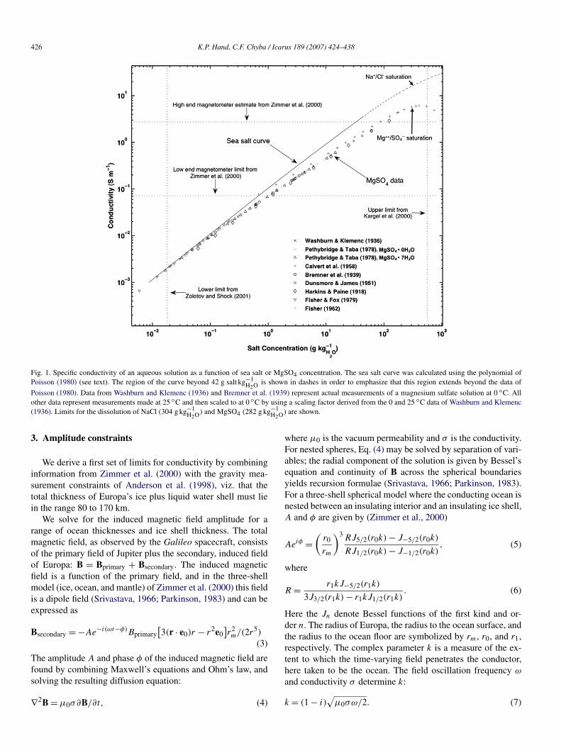
However, most models (Kargel et al., 2000; McKinnon andZolensky, 2003; Zolotov and Shock, 2001) as well as aque-ous leaching experiments (Fanale et al., 2001) suggest MgSO4,not NaCl, as the dominant salt in Europa’s ocean. There-fore, we have searched the literature to obtain concentration–conductivity data for MgSO4. In Fig. 1 we plot the available

conductivity–concentration data for MgSO4 along with, forcomparison, Eq. (1) for terrestrial ocean conductivity–salinity.Fig. 1 shows magnetometer constraints for conductivity as wellas some published compositional model constraints on salin-ity. Conductivity data at 0 ◦C (Washburn and Klemenc, 1936;Bremner et al., 1939) have been combined with data takenat 25 ◦C (Calvert et al., 1958; Pethybridge and Taba, 1977;Dunsmore and James, 1951; Harkins and Paine, 1919; Fisher,1962; Fisher and Fox, 1979) that we have scaled to 0 ◦C bymultiplying the 25 ◦C conductivity data by a scaling factorof 0.525. This scaling is possible because Washburn and Kle-menc (1936) report conductivity–concentration data for both0 and 25 ◦C across the concentration range from 0.6 to 60 gMgSO4 kg−1

H2O. The scaling factor was calculated by finding theratio of conductivities for T = 0 and T = 25 ◦C for a given saltconcentration. The average of the nine ratios available from theWashburn and Klemenc (1936) data was used as our final scal-ing factor. The fact that the temperature-scaled data fall alongthe curve sketched by the more sparse Washburn and Klemenc’s(1936) 0 ◦C and the Bremner et al.’s (1939) 0 ◦C data suggestthat this temperature scaling has been done correctly. We fit athird-degree polynomial to the data,

(2)C = c3σ3 + c2σ

2 + c1σ + c0,

finding the coefficients, c3 = −1.7268, c2 = 12.0161, c1 =15.2108, c0 = −0.0129, where C is concentration and σ is con-ductivity. Errors for values calculated using the polynomial fitare on the order of a few percent across the range of conductiv-ities considered here.

From Eq. (2) or Fig. 1, we see that the lower conductivitylimit of 58 mS m−1 corresponds to a minimum MgSO4 con-centration of 0.91 g MgSO4 kg−1

H2O. With the added constraint

of a hydrosphere <200 km thick (σ > 72 mS m−1), we find aminimum salt concentration of 1.1 g MgSO4 kg−1

H2O. This valueis a factor of 50 greater than the lower limit partial extractionmodel of Zolotov and Shock (2001) so that the lowest extractionmodels are excluded by the data. The lower limit on σ proposedby Schilling and Neubauer (2005), based on longer period wavepropagation, requires 4.5 g MgSO4 kg−1

H2O. Zimmer et al. (2000)do not explicitly provide an upper limit to the conductivity ofthe ocean. However, they determine that an ocean of terrestrialsalinity (s = 35, or a concentration of 34 g sea salt per kg of wa-ter (kg−1

H2O) at 0 ◦C, corresponding to 2.75 S m−1) would implya near-surface ocean of only 3.5 km thickness. (An insulatingice shell is ignored in their model; they therefore treat the upper-most 3.5 km of Europa as conducting.) A shell of conductivity2.75 S m−1 would require 96.8 g MgSO4 kg−1

H2O.In summary, the range of empirically supported MgSO4

salt concentrations permitted by Fig. 1 and previously pub-lished conductivity constraints falls between 1.1 and 96.8 gMgSO4 kg−1

H2O. Note that the high-end value is not well con-strained by values in the literature. Therefore in subsequent sec-tions we work to provide a stronger constraint on this value andshow that empirical constraints from Galileo, combined withphysical limitations on the conductivity resulting from salinity,necessitate a thin ice shell.

426 K.P. Hand, C.F. Chyba / Icarus 189 (2007) 424–438

Fig. 1. Specific conductivity of an aqueous solution as a function of sea salt or MgSO4 concentration. The sea salt curve was calculated using the polynomial ofPoisson (1980) (see text). The region of the curve beyond 42 g salt kg−1

H2O is shown in dashes in order to emphasize that this region extends beyond the data of

Poisson (1980). Data from Washburn and Klemenc (1936) and Bremner et al. (1939) represent actual measurements of a magnesium sulfate solution at 0 ◦C. Allother data represent measurements made at 25 ◦C and then scaled to at 0 ◦C by using a scaling factor derived from the 0 and 25 ◦C data of Washburn and Klemenc(1936). Limits for the dissolution of NaCl (304 g kg−1

H2O) and MgSO4 (282 g kg−1H2O) are shown.

3. Amplitude constraints

We derive a first set of limits for conductivity by combininginformation from Zimmer et al. (2000) with the gravity mea-surement constraints of Anderson et al. (1998), viz. that thetotal thickness of Europa’s ice plus liquid water shell must liein the range 80 to 170 km.

We solve for the induced magnetic field amplitude for arange of ocean thicknesses and ice shell thickness. The totalmagnetic field, as observed by the Galileo spacecraft, consistsof the primary field of Jupiter plus the secondary, induced fieldof Europa: B = Bprimary + Bsecondary. The induced magneticfield is a function of the primary field, and in the three-shellmodel (ice, ocean, and mantle) of Zimmer et al. (2000) this fieldis a dipole field (Srivastava, 1966; Parkinson, 1983) and can beexpressed as

(3)Bsecondary = −Ae−i(ωt−φ)Bprimary

[3(r · e0)r − r2e0

]r2m/(2r5)

The amplitude A and phase φ of the induced magnetic field arefound by combining Maxwell’s equations and Ohm’s law, andsolving the resulting diffusion equation:

(4)∇2B = μ0σ∂B/∂t,

where μ0 is the vacuum permeability and σ is the conductivity.For nested spheres, Eq. (4) may be solved by separation of vari-ables; the radial component of the solution is given by Bessel’sequation and continuity of B across the spherical boundariesyields recursion formulae (Srivastava, 1966; Parkinson, 1983).For a three-shell spherical model where the conducting ocean isnested between an insulating interior and an insulating ice shell,A and φ are given by (Zimmer et al., 2000)

(5)Aeiφ =(

r0

rm

)3 RJ5/2(r0k) − J−5/2(r0k)

RJ1/2(r0k) − J−1/2(r0k),

where

(6)R = r1kJ−5/2(r1k)

3J3/2(r1k) − r1kJ1/2(r1k).

Here the Jn denote Bessel functions of the first kind and or-der n. The radius of Europa, the radius to the ocean surface, andthe radius to the ocean floor are symbolized by rm, r0, and r1,respectively. The complex parameter k is a measure of the ex-tent to which the time-varying field penetrates the conductor,here taken to be the ocean. The field oscillation frequency ω

and conductivity σ determine k:

(7)k = (1 − i)√

μ0σω/2.


Fig. 2. Ocean depth–salt concentration relationship for an induced magnetic field amplitude of A = 0.7. Magnesium sulfate concentrations (g per kg water) forvarying ocean thicknesses were calculated (see text) for a variety of ice shell thicknesses. The plot shows lines of constant ice thickness. Starting from the left, linesare given for no ice shell (0 km) on up to a 50 km ice shell, in 10 km increments. The inset plot details the 50–180 km ocean thickness region and shows lines of iceshell thickness ranging from 0 to 50 km in 5 km increments. All of the solutions shown in the inset plot would be considered freshwater, or nearly freshwater (i.e.oligohaline or mildly brackish), by Earth standards.

We calculate A for a range of ocean thicknesses, ice thick-nesses, and ocean conductivities. In this first model, the ice shelland mantle are assumed to have zero conductivity; we solve fora conductive mantle later in this work. For small σ (�1 S m−1)

we solve for A exactly. As σ increases, however, the terms inthe numerator and denominator of Eq. (5) rapidly approachzero, creating a region of numerical instability. For large σ

we use an approximation to Eq. (5) wherein the highest-order(smallest) terms are discarded. The full approximation is de-tailed in Appendix A; we demonstrate there that it is a goodapproximation for σ � 0.1 S m−1.

Zimmer et al. (2000) concluded that induced field ampli-tudes of A < 0.7 are hard to reconcile with the Galileo observa-tions; so in all cases we have solved for conductivity variationswith A � 0.7. Furthermore, amplitudes for A > 1.0 imply sig-nificant conductivity outside the moon (e.g. ionosphere, cloudof pick-up ions) and Zimmer et al. (2000) argue that the ob-served magnetic signature does not fit such a model. We never-theless address the possible contribution of an ionosphere in asubsequent section. More recent work using a least-squares fitto the magnetometer data (Schilling et al., 2004) concludes thatA = 0.97±0.02. Here we examine how variations in the ampli-tude A, coupled with variations in the ice shell and ocean thick-nesses, constrain the salt concentration in the putative ocean.

3.1. Amplitude response A � 0.9

First, we examine the low-end case of A = 0.7. Results areshown in Fig. 2. The range of ocean thicknesses shown in Fig. 2covers the range allowed by the gravity data (Anderson et al.,1998). Lines of constant ice shell thickness are shown for shellsranging from 0 to 50 km thickness. For the case of a 100 kmthick ocean with ice shells of different thicknesses, the resultingsalt concentrations all fall below 2.7 g MgSO4 kg−1

H2O. Note thateven for the case of a 50 km ice shell overlying a 50 km ocean,the required salt concentration when A = 0.7 still falls below5 g MgSO4 kg−1

H2O.Considering some of the cases permitted by the two ex-

tremes of the gravity data, we have calculated that a 160 kmliquid water ocean beneath a 10 km ice shell would require aconcentration of 1.3 g MgSO4 kg−1

H2O (σ ∼ 88 mS m−1). Simi-larly, for the lower-limit case of an 80 km hydrosphere, we findthat a 60 km thick ice shell with a 20 km liquid water con-ducting layer at the bottom would require 15.6 g MgSO4 kg−1

H2O

(σ ∼ 0.69 S m−1) whereas an ice shell of 10 km with a 70 kmocean requires only 2.8 g MgSO4 kg−1

H2O (σ ∼ 165 mS m−1).That is, for the case of A = 0.7, even the extreme choices per-mitted by the gravity data give low MgSO4 concentrations, inthe range 1 to 16 g kg−1 .
H2O


Fig. 3. Ocean depth–salinity relationship for an induced magnetic field amplitude of A = 0.8. Magnesium sulfate concentrations (g per kg water) for varying oceanthicknesses were calculated (see text) for a variety of ice shell thicknesses. The plot shows lines of constant ice thickness. Starting from the left, lines are given forno ice shell (0 km) on up to a 50 km ice shell, at 10 km increments.

As we increase the amplitude response, A, the conductivelayer approaches a perfect conductor (A = 1.0). Solutions forA = 0.8 and A = 0.9 are shown in Figs. 3 and 4, respectively.Examining the case of a 10 km ice shell overlying a 100 kmthick ocean, we find that for A = 0.8 the required salt con-centration is 3.2 g MgSO4 kg−1

H2O while for A = 0.9, the re-

quirement increases to 10 g MgSO4 kg−1H2O. Both values are still

significantly lower than the sea salt concentration of the terres-trial ocean. Increasing the ice shell to 50 km thickness pushesthe salt concentration up to 5.6 g MgSO4 kg−1

H2O for the caseof A = 0.8. Under the same circumstances, raising A to 0.9 re-quires increasing the conductivity to ∼175 S m−1 (see Fig. 5).This value is far beyond the conductive capabilities of salt ionsin water, so these parameter combinations are not permitted. Weexplore these issues in depth in subsequent sections.

3.2. Amplitude response A = 0.97 ± 0.02

As A increases toward 1.0, salt concentrations must con-comitantly increase. While Zimmer et al. (2000) argued thatA must lie in the range 0.7 � A � 1.0, more recent work bySchilling et al. (2004) suggests that A = 0.97 ± 0.02. In Figs. 5and 6 we extend the range of conductivities to include large val-ues for σ and we show how the combination of ocean thickness,

ice shell thickness, and conductivity determine the amplitude ofthe induced magnetic field. We explore the range of physicallyplausible conditions that could allow such a high value of A.Ultimately we show that because there is an upper limit on theconductivity of the ocean placed by the salt ion saturation, val-ues of A = 0.97 ± 0.02 are only possible if the ice shell is thin.

In Fig. 5, three models for the ocean thickness are consid-ered: 80, 100, and 120 km, and in each case we examine thesolutions for ice shell thicknesses of 0, 10, 30, and 50 km. Atconductivities below 1.2 S m−1 the ocean thickness plays animportant role in determining the amplitude. However, beyond1.2 S m−1 the ice shell thickness dominates the amplitude re-sponse. As shown in Fig. 5, when σ > 2 S m−1 ice shells ofgreater thickness require higher oceanic conductivities in or-der to achieve the same amplitude response. As conductivityincreases, the amplitude slowly approaches the idealized per-fect conductor case of A = 1.0. Here we solve for values ofσ up to 300 S m−1 (∼120 times the conductivity of Earth’socean), at which point the maximum achievable amplitude re-sponse is A = 0.99. This is for no ice shell (d = 0), obviouslynot physically plausible. If we instead consider the case ofd = 10 km, then at σ = 300 S m−1 we find A = 0.97. Similarly,for d = 30 and d = 50 km we find A = 0.94 and A = 0.90, re-spectively.


Fig. 4. Ocean depth–salt concentration relationship for an induced magnetic field amplitude of A = 0.9. Magnesium sulfate concentrations (g per kg water) forvarying ocean thicknesses were calculated (see text) for a variety of ice shell thicknesses. The plot shows lines of constant ice thickness. Starting from the left, linesare given for no ice shell (0 km), a 10 km shell, and a 20 km shell. The double-valued shape of the curves is due to skin depth effects in amplitude and phase (seetext).

In practice there are physical limits on how much salt canbe added to water and thus there are limits to how high theconductivity can be driven by the concentration of salt ions.Saturation for the dissolved ionic form of MgSO4 occurs at∼282 g MgSO4 kg−1

H2O (Hogenboom et al., 1995; Kargel, 1991)

and for NaCl saturation occurs at ∼304 g NaCl kg−1H2O at 25 ◦C

(Oren, 2001). Hydrated forms of MgSO4 may exist in suspen-sion in the water (e.g. MgSO4·7H2O), but these forms do notcontribute to the conductivity of the ocean water. In addition,as the salt concentration increases the viscosity of the solutionalso increases, reducing the mobility of the ions and limitingthe conductivity (Anderko and Lencka, 1997). At low tem-peratures, increasing pressure over the range 0–400 MPa haslittle effect on conductivity (Quist and Marshall, 1968). The∼5–200 MPa range within Europa’s ocean should thus causelittle variation in conductivity. Hypersaline environments onEarth are rarely above a few Siemens per meter. For example,the brine of Mono Lake in Northern California is reported tobe 8.57 S m−1 (at 25 ◦C) (Jellison et al., 1999), and the brinesaturated sediments of Lake Magadi in Southwest Kenya aremeasured to be ∼11 S m−1 (34 ◦C) (Jones et al., 1998).

The saturation limits for salt concentration impose limitson the conductivity (∼6 S m−1 for MgSO4 and ∼18 S m−1

for sea salt) that are hard to reconcile with the high ampli-tude requirement of A ∼ 0.97. In Fig. 5 we show the upperlimit for conductivity of an MgSO4 or NaCl solution. As isshown, the intersection of these lines with A = 0.97 yields anice shell of thickness equal to, or less than, 4 km. Taking thelower end of the error bar, A = 0.95, we find that at most theice shell is 7 km (MgSO4) to 15 km (NaCl) thick. Even if asolution of conductivity 30 S m−1 were physically plausible,we would still have upper limits on the ice shell thickness of∼6 and ∼17 km for A = 0.97 and A = 0.95, respectively (forNaCl). Additionally, it should be noted that salt concentrationsof �300 g per kg of H2O would push the density of the solutionbeyond those permissible by the three-shell internal modelingresults of Anderson et al. (1998). This density constraint is notterribly strict—alternative interior models fitting for the bulkdensity and moment of inertia could allow for higher densityouter shells—but it does provide another piece of informationpertaining to the bulk properties of putative ocean.

Does the above analysis demonstrate that Europa’s ice shellmust be �15 km? While Schilling et al. (2004) conclude thatA = 0.97 ± 0.02, this value is derived by comparing two differ-ent models for the external and internal magnetic fields in andaround Europa. In the first case, Europa is allowed to have an


(a)

(b)

Fig. 5. Amplitude, A, as a function of conductivity, ocean thickness, and ice shell thickness. At low conductivities the ocean thickness dominates the amplituderesponse, however, as the conductivity of the solution increases, ocean thickness becomes less important and the thickness of the non-conducting ice shell dominatesthe inductive amplitude response. (a) Three-layer spherical model with non-conducting ice shell and mantle. The only solutions consistent with the magnetometerdata [Schilling et al. (2004) require A = 0.97±0.02] and the gravity data (Anderson et al., 1998) are those in which the ice shell is thin (between 0 and 15 km thick).The optimal fit for an ocean dominated by NaCl is 4 km thickness. The maximum allowable ice shell thickness for an MgSO4 dominated ocean is 7 km. (b) Five-layerhalf-space model. Results are very similar to the three-layer spherical model. Values for the conductivity of individual layers are: σIonosphere = 2 × 10−4 S m−1;

σIce = 1 × 10−10 S m−1; σMantle = 0.01 S m−1; σCore = 3.3 × 105 S m−1. Again the optimal fit to the magnetometer data is achieved with a 4 km thick ice shell.The maximum thickness allowed by the error bars is 16 km, slightly more than calculated with the three-layer spherical model. This difference is primarily due toconductivity limits for the half-space model (see text).


(a)

(b)

Fig. 6. Contours of conductivity as a function of amplitude and ocean thickness. In (a), the ice thickness in all cases is assumed to be 10 km. In (b), the ice thicknessin all cases is assumed to be 30 km.

internal permanent dipole moment with a surface magnitude of23 nT and a tilt of 59◦ from the Europa’s spin axis. From thisfit to the magnetometer data, they find that A = 0.96 ± 0.03. Inother words, if we allow Europa to have an internal magneticfield, we can push the amplitude down to 0.93. Even for thislow of a value for A, we find that the ice shell must be equal to,or less than 26 km thick. In their model without an internal di-pole, Schilling et al. (2004) find that A = 0.98 ± 0.01. Here thelower limit of A = 0.97 again leads us to an ice shell of �4 kmfor the case of NaCl. At A = 0.98, the ice shell can be only me-ters thick. Ultimately, the work of Schilling et al. (2004) is datalimited—only four Galileo passes of Europa were close enoughto satisfy their criterion. However, in their rigorous analysis and

fitting of models so as to minimize root-mean square fits to thedata, they conclude that A = 0.97±0.02, taking all models intoaccount. In this case, the ice must indeed be �15 km.

In Fig. 6 we show how varying the ocean thickness affectsthe amplitude response. Contours for the saturation limits onconductivity, along with several other conductivity contours ofinterest are shown. In Fig. 6a the ice shell thickness is 10 km,whereas in Fig. 6b the ice shell is 30 km thick. These contoursreveal that for conductivities of a few Siemens per meter the in-ductive response actually decreases as we increase the thicknessof the conducting layer (i.e. the ocean thickness). This is likelya skin depth effect, and can be understood semi-quantitativelyin the following way. In the case of a plane conductor, the solu-


tion to Eq. (4) is simply (e.g. Parkinson, 1983):

(8)B = B0e−z/δe−i(ωt−z/δ),

where z = 0 at the boundary of the conductor and increasespositively into the conductor, and

(9)δ = (μ0σω/2)−1/2

is the skin depth. For every increment δ of depth z into the con-ductor, the amplitude decreases by a factor of e and the phasechanges by one radian. Therefore, increasingly deep layers ofthe conductor both contribute less to the amplitude, and con-tribute increasingly destructively (out of phase). For σ = 1 and10 S m−1, δ = 101 and 32 km, respectively, consistent with thebehavior seen in Figs. 3–6.

Of course, a nested spherical shell model for Europa requiresthat Eq. (4) be solved in spherical coordinates, and the solutionis Eq. (5), not Eq. (8). However, Eqs. (8) and (9) will providea good local approximation for the solution into the sphericalconductor provided that (Srivastava, 1966)

(10)σ � 2/(μ0ωr2).

In this case, the real part of kr � 1, allowing us to drop thefirst derivative term in the Bessel equation solution to the ra-dial part of Eq. (4), and the system has solutions given byEqs. (8) and (9) (Srivastava, 1966). For Europa, r = 1560 kmand ω = 2π/P = 1.6×10−4, where P = 4.03×104 s = 11.2 his Jupiter’s synodic rotation period. Equation (10) will thereforehold when σ � 10−3 S m−1, which will be the case for the con-ductivities of interest here. Therefore Eqs. (8) and (9) providegood insight into the decay and phase change of the magneticfield as it extends down into Europa’s ocean.

For certain combinations of σ and ocean thickness, the in-duced response at depth will cancel part of the induced re-sponse generated near the surface; this behavior explains, e.g.,the shape of the curves in Fig. 6. For large conductivity theskin depth goes to zero—all of the induced response is gen-erated near the surface—and cancellation effects are avoided.A curious consequence of this behavior is that if the salinity ofthe putative europan ocean is comparable to that of the Earth’socean (with σ of a few S m−1), then thinner oceans provide abetter fit to the high amplitude requirement of Schilling et al.(2004).

Table 1 summarizes the relationship between layers on our3-layer model, providing values of A for a variety of plausiblecombinations of ice thickness, ocean thickness, and conductiv-ity. Again, A can only exceed 0.95 for thin ice shells and near-saturation salt concentrations, regardless of which scenario isconsidered.

4. Adding a conducting core, mantle, and ionosphere

We have shown that the three-layer model can only fit themagnetometer amplitude constraints if the conductivity is highand the ice shell thin. Here we explore the influence of a con-ducting ionosphere, mantle, and core on the induced field re-sponse. We use a plane stratified half-space (Parkinson, 1983;

Srivastava, 1965) instead of a spherical model. As previouslyshown, this model is a good approximation for Europa for con-ductivities greater than approximately 10−3 S m−1. This leadsto a planar approximation with m shells and a recursive ex-pression for the ratio of the induced to external fields givenby

(11)Bi

Be

= R1(α1 − ν) − α1 − ν

R1(α1 + ν) − α1 + ν,

where

(12)Rj = e2αj zjRj+1(αj + αj+1) + (αj − αj+1)e

2αj+1zj

Rj+1(αj − αj+1) + (αj + αj+1)e2αj+1zj

,

and the recursion is initiated by

(13)Rm−1 = e2αm−1zm−1(αm−1 + αm)

(αm−1 − αm).

Here αm = √ν2 + k2

m, where km is given by (7) and ν is a con-stant resulting from separation of variables when solving thehalf-space model (Price, 1962). Physically, the value 2π/ν isa measure of the horizontal scale and uniformity of the sourcefield (Srivastava, 1965; Price, 1962), with ν = 0 representingno spatial variation in the field (Cagniard, 1953). Price (1962)however showed that even very small values of ν are impor-tant for accurate modeling. For the case of the Earth, Pricefinds the smallest permissible value of ν to be found by set-ting 2π/ν equal to the circumference of the Earth. The largestvalue is found by setting 2π/ν equal to a few times the height ofthe terrestrial ionosphere. Following Srivastava (1965) we takeν = [n(n + 1)]1/2/rEuropa, where n is the order of the Besselfunction, so n = 1 for the external dipole field. This leads to agood match with the 3-layer spherical model, though for thickice shells (>30 km) the results yield slightly higher values forthe amplitude. This is in part due to the fact that adding thevery low-conductivity ice layer means adding a layer that doesnot satisfy the conductivity criteria for the half-space model.The net effect is that our 5-layer model over-estimates the am-plitude response and consequently over-estimates the ice shellthickness. Even so, the 5-layer model still predicts an ice shellof <16 km, with a best-fit at 4 km. Fig. 5b shows these re-sults.

In Fig. 7 we show amplitude profiles for several differentcombinations of ionosphere, mantle, and core conductivity. Forocean conductivities greater than ∼3 S m−1, the contributionfrom these additional layers is negligible. Below this value,the core and mantle are seen to have a strong influence onamplitude. The effect of induction in the core and mantle is pri-marily deconstructive interference with induction in the ocean.The result is that for a given ocean conductivity, a conductivecore (and/or mantle) lowers the amplitude response of the to-tal induced field. Values for both layer conductivity and layerthickness were varied based on published estimates (Zimmeret al., 2000; Saur et al., 1998; Parkinson, 1983; Petrenko andWhitworth, 1999; Anderson et al., 1998; Stacey, 1992). Thoughwe have shown results for mantle conductivity of 200 S m−1

(dash-dotted line) this is a very high-end value that wouldlikely only persist for the upper few kilometers of oceanic crust.


Table 1Induced amplitude response

Oceanthickness(km)

Icethickness(km)

Amplitude of induced magnetic field (A)

Salt concentration (g salt kg−1H2O) [conductivity, S m−1]

1.14 [0.072] 5.0 [0.25] 100 [3.0] 282 [6.0] 304 [18.0] 350 [23.0]

60 0 0.38 0.80 0.96 0.97 0.98 0.9810 0.37 0.78 0.94 0.95 0.96 0.9630 0.35 0.75 0.91 0.91 0.92 0.9250 0.33 0.71 0.87 0.88 0.89 0.89

80 0 0.46 0.84 0.95 0.96 0.98 0.9810 0.45 0.83 0.94 0.94 0.96 0.9630 0.43 0.79 0.90 0.91 0.92 0.9250 0.41 0.76 0.86 0.87 0.87 0.89

100 0 0.53 0.87 0.95 0.96 0.98 0.9810 0.52 0.85 0.93 0.94 0.96 0.9630 0.49 0.81 0.89 0.91 0.92 0.9250 0.47 0.78 0.86 0.87 0.89 0.89

120 0 0.59 0.88 0.95 0.96 0.98 0.9810 0.57 0.86 0.93 0.94 0.96 0.9630 0.54 0.82 0.89 0.91 0.92 0.9250 0.52 0.79 0.86 0.87 0.89 0.89

150 0 0.64 0.88 0.95 0.96 0.98 0.9810 0.63 0.86 0.93 0.94 0.96 0.9630 0.60 0.82 0.89 0.91 0.92 0.9250 0.57 0.79 0.86 0.87 0.89 0.89

Note. Induced amplitude response, A, is provided for a variety of MgSO4 concentrations, ocean thicknesses, and ice shell thicknesses. The salt concentrations shownhere correspond to: (1) the low-end conductivity limit of Zimmer et al. (2000); (2) the low-end conductivity limit of Schilling and Neubauer (2005); (3) the high-endestimate for MgSO4 concentration of McKinnon and Zolensky (2003); (4) the ionic saturation concentration for MgSO4; (5) the saturation concentration of NaCl;and (6) the density limit for the water layer on Europa (Anderson et al., 1998). Errors in the salt concentration, primarily resulting from the polynomial fit, are onthe order of ±0.1 g MgSO4 kg−1

H2O.

Measurements of terrestrial mantle conductivity suggest thata ∼600 km thick mantle would likely have a bulk conductiv-ity in the range of 0.01 S m−1 (solid line) (Parkinson, 1983;Stacey, 1992). Comparisons with electrical properties of chon-drites indicate that such conductivities are also compatible witha mantle of chondritic origin (Campbell and Ulrichs, 1969).Thus, as is shown in Fig. 7, we expect that on Europa the am-plitude response at low ocean conductivities will be dominatedby the core. In all cases, we find that adding conductive man-tle and core layers to our model does not significantly influencethe amplitude response in the region where A = 0.97 ± 0.02.

The case of a conducting ionosphere is treated separately.First we note that in order to properly compare the amplitude re-sponse with and without an ionosphere, we must scale the mod-els with an ionosphere by a factor of ∼(r0/rm)3. Here r0 is thetotal thickness and rm is the thickness without the ionosphere.This scaling normalizes A for thickness variations between themodels, and in so doing reveals amplitude differences resultingfrom ionospheric conductivity. The scaling factor allows us tocompare with published values of A, all of which are calculatedfor Bind/Bext at the surface of Europa. The cube of the ratio ac-counts for the 1/r3 change in the external and induced fields asone moves from the ice surface to the top of the ionosphere. Thescaling factor is chosen such that at zero ionospheric conductiv-ity, the ratio of the amplitudes for models with and without anionosphere is one.

Estimates for ionospheric conductivity range from <5 ×10−5 to 2 × 10−4 S m−1 (Khurana et al., 2002; Saur et al.,1998; Zimmer et al., 2000). We take 300 km as our nominalionosphere thickness (Zimmer et al., 2000), but we find thatthis parameter can be changed without impacting the results,provided the conductivity is constrained to the range above.

Fig. 8 shows that even with the high-end value of 2 ×10−4 S m−1 for ionospheric conductivity, there is negligible ef-fect on the amplitude response. Only when the conductivity isapproximately two orders of magnitude higher do we see signif-icant changes in the amplitude response. In Fig. 9 we show thisrelationship by plotting the conductivity of the ionosphere ver-sus the ratio of the amplitudes for a model with an ionosphereto that without a conducting ionosphere. At high conductiv-ities for the ionosphere, the amplitude ratio becomes greaterthan one, indicating that the ionosphere could drive the ampli-tude response to very high values if such conductivities werephysically plausible. Only when the ocean conductivity is verylow (e.g. 0.1 S m−1) do we begin to see some influence of theionosphere at realistic values for ionospheric conductivity. Eventhen, the net effect does not help us resolve the issue of theobserved high values for the amplitude response. At very lowocean conductivities a conducting ionosphere can influence theamplitude response, but since the ocean conductivity is so low,the amplitude response is limited to values below A ∼ 0.7. Inother words, adding a conductive ionosphere could alter our in-


Fig. 7. Adding a conducting core and mantle influences the total amplitude response when the ocean conductivity is small. Even for models with a very conductingcore and mantle, the amplitude in the region A � 0.95 is dominated by the conductivity of the ocean and the ice shell thickness.

Fig. 8. Adding an ionosphere to our model results in little change to the amplitude profile for all reasonable values of ionospheric conductivity (�2 × 10−4 S m−1).The dashed lines show results for models with an ionosphere of conductivity 2×10−4 S m−1 and the solid lines show results for an ionosphere of zero conductivity.As shown by the dotted line, it is only when the ionosphere reaches physically implausible levels of conductivity that an influence on the amplitude is observed. Inall cases the ionosphere is 300 km thick, the ice has zero thickness, and the ocean is 100 km thick. The amplitude has been normalized for comparison to publishedvalues of A (see text).


Fig. 9. Comparison of amplitudes, A, for models with and without conducting ionosphere. Here we define the ratio of the amplitudes as AIC/AI0, where AICis the amplitude for a model with a conducting ionosphere and AI0 is the amplitude for a model without a conducting ionosphere. We then plot this ratio asa function of ionospheric conductivity for several different choices of ocean conductivity. In all cases the ratio is very close to unity for reasonable choices ofionospheric conductivity (�2 × 10−4 S m−1). The ionosphere shows a stronger effect for small values of ocean conductivity; however, such low values for theocean conductivity are not consistent with the empirical constraints on the observed amplitude (Zimmer et al., 2000; Schilling et al., 2004).

terpretation of the broad range of allowed amplitudes, 0.7 <

A < 1.0 (Zimmer et al., 2000), but it has no influence whenconsidering the much tighter constraints, A = 0.97 ± 0.02, ofSchilling et al. (2004).

In summary, even when we add a conducting core, mantle,and ionosphere, we find that the critical factors for achievinghigh values of A are the ocean conductivity and ice shell thick-ness.

5. Implications for ice shell thickness

We have shown that for the lower end limits of the Zimmeret al. (2000) model (0.7 < A < 0.9) many of the most plausiblesolutions yield oceanic salt concentrations of less than ∼15 gMgSO4 kg−1

H2O, and solutions of <3 MgSO4 kg−1H2O are entirely

possible. In other words, by terrestrial standards, the putativeocean of Europa could be much less saline than our ocean andfor some solutions it could even qualify as a freshwater ocean.

However, given the interplay of the conductivity, oceanthickness, and ice shell thickness in this model, we find thatin order to satisfy the Galileo-constrained amplitude responseof A = 0.97 ± 0.02 (Schilling et al., 2004), the ice shell mustbe �15 km thick, irrespective of ocean thickness. For an iceshell of near-zero conductivity (σIce = 1 × 10−10 S m−1), wefind that an ice shell thickness of ∼4 km—comparable to thatof the Antarctic ice sheet—best satisfies the A = 0.97 require-ment. Even if we account for changes in the ice shell conduc-

tivity resulting from variations in temperature with depth, al-lowing the conductivity to reach ∼10−4 S m−1 (Addison, 1969;Moore et al., 1994), we find no change in our results.

For a three-shell gravity model, the combined ocean plus icethickness must be greater than 80 km (Anderson et al., 1998),thus implying an ocean at least 70 km thick. Trading liquid wa-ter for ice (e.g. 50 km water and 30 km ice) results in a pooramplitude response, one only satisfied by the lower end fits tothe Galileo magnetometer data (Zimmer et al., 2000). If oneconsiders the MgSO4 constraints suggested by McKinnon andZolensky (2003) of <100 g MgSO4 kg−1

H2O, it is then impossi-ble to satisfy the A ∼ 0.97 constraint of Schilling et al. (2004)with the model of Zimmer et al. (2000). At 100 g MgSO4 kg−1

H2O

(∼3.0 S m−1) the largest amplitude response is A = 0.94 whenthe ice shell thickness is set to zero.

An upper limit on salinity is set by the saturation limits ofthe various salt ions. With Mg2+ and SO2−

4 as the primarycation and anion, saturation is reached at approximately 282 gMgSO4 kg−1

H2O in Europa’s ocean. If more MgSO4 is added itforms a hydrate and does not dissolve. Models of plume cur-rents in the europan ocean indicate that such material is unlikelyto remain in suspension and will most likely precipitate to theocean floor (Goodman et al., 2004). Consequently, adding morethan 282 g MgSO4 kg−1

H2O does not help explain the inducedmagnetic field response of Europa. The conductivity can bepushed higher by considering sea salt (e.g. Na+ and Cl−), but


even then the conductivity of the solution will not exceed tens ofSiemens per meter. As a result, invoking a salty ocean to explainthe observed induced magnetic field fails unless the ice shell isthin or the amplitude is less than that determined by Schillinget al. (2004). In order to have a thick ice shell (�30 km), theinduced amplitude must be less than 0.92, contradictory to theresults of Schilling et al. (2004).

6. Implications for habitability

If the ice and liquid water layers on Europa fall withinthe limits of Fig. 2 (A = 0.7) then, by standard definitionsof “freshwater” environments on Earth [broadly meaning<3 g salt kg−1

H2O (Barlow, 2003)], Europa’s ocean would be afreshwater ocean, though admittedly more salty than most ter-restrial lakes. Indeed, in this case, the putative global ocean ofEuropa could be more like the mildly saline environment ofPyramid Lake, Nevada than like the Earth’s ocean. While thedrinking water regulations of the U.S. Environmental Protec-tion Agency recommend no more than 0.25 g of sulfate perkilogram of water, adult humans can acclimatize to drinkingwater with nearly 2 g MgSO4 kg−1

H2O without much discomfort(EPA, 2004; CDC-EPA, 1999). Animal toxicity (the lethal dosefor 50% of the population) is in the range of 6 g MgSO4 kg−1

H2O(CDC-EPA, 1999), but most livestock are satisfied provided thetotal salt concentration is less than 5 grams per kilogram of wa-ter (ESB-NAS, 1972). If we assume the low amplitude regimefor our solution (A < 0.8) then it is possible that human or beastcould drink the water of Europa.

What are the implications for habitability for A = 0.97? Ter-restrial halophilic microorganisms are capable of surviving atNaCl saturation (Oren, 1994, 2002). Among these are microbesfrom each domain of life (Archaea, Bacteria, and Eucarya).Metabolic pathways for these microbes include oxygenic andanoxygenic photosynthesis (Dunaliella salina, Halorhodospirahalphila), aerobic respiration (Halobacterium salinarum), andfermentation (Halobacterium salinarum). Obviously, photo-synthesis is an unlikely metabolic pathway if the ice is morethan a few tens of meters thick, but respiration and fermentationcould be possible, especially if radiolytically produced oxidantsare delivered to the sub-surface (Chyba, 2000; Chyba and Hand,2001). Methanogens—sometimes considered a plausible modelfor europan life (McCollom, 1999)—are capable of survivingin solutions near NaCl saturation if methanol or methylatedamines are available (Oren, 2001). Data for MgSO4 toleranceis limited, but microbes such as Halobacterium sodomense areknown to survive in solutions above 2 M Mg2+ (equivalent to∼260 g MgSO4 kg−1

H2O) (Oren, 1994). Thus on Europa, wherethe high amplitude constraint necessitates a high salt concen-tration, the habitability of the ocean may be limited but theconditions would not appear to exclude life as we know it.

But habitability for life is not the same as suitability forthe origin of life. Experimental investigations of the influenceof ionic inorganic solutes on self-assembly of monocarboxylicacid vesicles, and the nonenzymatic, nontemplated polymeriza-tion of activated RNA monomers may support the contentionthat life originated in a freshwater solution (Monnard et al.,

2002). In these prebiotic simulation experiments, sodium chlo-ride or sea salt concentrations as low as 25 mM NaCl (1.5 gper kg of H2O) were found to “substantially” reduce oligomer-ization, with higher concentrations having worse effects. Butthese experiments have not yet been performed with MgSO4.With regard to vesicle formation, if the ratio of the cation to am-phiphile falls below ∼1, then it becomes possible for the excessamphiphile to form membranes; above ∼2 and the amphiphileprecipitates and no membrane formation occurs. The Monnardet al.’s (2002) results therefore suggest that the upper rangeof salinities implied by the Galileo magnetometer experimentscould pose a serious challenge to the origin of life in Europa’sbulk contemporary ocean, were abiotic RNA oligomerization oramphiphile membrane formation on the critical path to the ori-gin of life, and if the experimental results for NaCl carry overto MgSO4.

7. Conclusion

Aside from surface imagery, the magnetometer results arethe only dataset that provides information about the relation-ship between the ice shell and putative subsurface ocean. In theanalyses presented here we have provided empirical constraintson both the salinity of the europan ocean and the overlyingice shell thickness. By the low-end, poorly constrained analysiswhere 0.7 � A � 1.0 (Zimmer et al., 2000) we find that a fresh-water ocean is possible on Europa. By the tighter Schilling etal. (2004) constraints of A = 0.97 ± 0.02, our results show thatan ice shell of thickness �4 km, overlying a very salty ocean,is the best fit to the data. Thicknesses ranging from 0 to 15 kmare permissible if one allows for the ±0.02 uncertainties in themagnetic field signature. These results apply to present day Eu-ropa and are independent of any geological interpretation ofsurface features.

While our work provides new insight into the nature of theice shell and ocean, we note two limiting factors in our mod-els, the first of which is the focus of subsequent studies. First,we have assumed that the bulk ocean temperature is ∼273 K.For a given salt concentration, higher temperatures would meanhigher conductivity. If the ocean is stratified and contains layersof significant thickness with temperatures slightly higher than273 K, then such layers would have slightly higher conductivity.Using this relationship, a magnetometer on a future spacecraftmission could potentially help determine ocean structure andtemperature profile.

The second limiting factor is simply the constraint on theamplitude. With additional analysis of the Galileo data, somegreater resolution on this issue may be achieved. However, finalanswers to the questions of Europa’s ice shell thickness, oceanchemistry, and habitability, await a future spacecraft mission.

Acknowledgments

We thank K. Khurana and J. Goodman for thorough andinsightful reviews. We also thank M. Cepuran, M. Kivelson,D. Deamer, R. Carlson, A. Goldman, T. Hoehler, J. Kargel, andP. Monnard for helpful discussions. This research was funded in


part by the NASA Astrobiology Institute and the NASA Grad-uate Student Researchers Program.

Appendix A

The approximation used to calculate the amplitude, A, forlarge values of conductivity, σ , was derived by eliminatingterms of order x2 and higher in the denominator of Eq. (5),where x = r0k or r1k. With this approximation, Eq. (5) simpli-fies to

Aeiφ ≈(

r0

rm

)3(

r1(r0 − (

r0r1k3

)tan(k(r0 − r1))

) − 1

)

(A.1)+ O

(1

x2

).

All variables are as defined in the text. Using Eq. (7) and an11.2-h synodic period for the primary field oscillation, we find

(A.2)|x| = r0|k| ≈ r1|k| ≈ 10σ 1/2,

with σ in S m−1. Therefore O(1/x2) ≈ 10−2σ−1 (σ in S m−1),and Eq. (A.1) is a good approximation to Eq. (5) providedσ > 0.1 S m−1. Explicit numerical ratioing of A from Eq. (A.1)to A from Eq. (5) verifies this analytical prediction. The so-lution for A is found by expanding Eq. (A.1) into real andimaginary components, and then eliminating φ in order to solvefor A. Figs. 2–4 were plotted using the exact solution for A,whereas in Fig. 5 we use the above approximation.

References

Addison, J.R., 1969. Electrical properties of saline ice. J. Appl. Phys. 40 (8),3105–3114.

Anderko, A., Lencka, M.M., 1997. Computation of electrical conductivity ofmulticomponent aqueous systems in wide concentration and temperatureranges. Ind. Eng. Chem. Res. 36, 1932–1943.

Anderson, J.D., Schubert, G., Jacobson, R.A., Lau, E.L., Moore, W.B., Sjogren,W.L., 1998. Europa’s differentiated internal structure: Inferences from fourGalileo encounters. Science 281, 2019–2022.

Barlow, P.M., 2003. Ground Water in Freshwater–Saltwater Environments ofthe Atlantic Coast. Department of the Interior, US Geological Survey, Re-ston. Circular 1262, p. 121.

Bremner, R.W., Thompson, T.G., Utterback, C.L., 1939. Electrical conduc-tances of pure and mixed salt solutions in the temperature range 0 to 25◦ .J. Am. Chem. Soc. 61, 1219–1223.

Cagniard, L., 1953. Basic theory of the magnetotelluric method of geophysicalprospecting. Geophysics 18, 605–635.

Calvert, R., Cornelius, J.A., Griffiths, V.S., Stock, D.I., 1958. The determinationof the electrical conductivities of some concentrated electrolyte solutionsusing a transformer bridge. J. Phys. Chem. 62, 47–53.

Campbell, M.J., Ulrichs, J., 1969. Electrical properties of rocks and their signif-icance for lunar radar observations. J. Geophys. Res. 74 (25), 5867–5881.

Carlson, R.W., Johnson, R.E., Anderson, M.S., 1999. Sulfuric acid on Europaand the radiolytic sulfur cycle. Science 286, 97–99.

CDC-EPA, 1999. Health Effects from Exposure to Sulfate in Drinking WaterWorkshop, EPA 815-R-99-002. Centers for Disease Control & US Environ-mental Protection Agency, Office of Water, Atlanta.

Chyba, C.F., 2000. Energy for microbial life on Europa. Nature 403, 381–382.Erratum in Chyba, C.F., 2000. Nature 406, 368.

Chyba, C.F., Hand, K.P., 2001. Life without photosynthesis. Science 292,2026–2027.

Dalton, J.B., Mogul, R., Kagawa, H.K., Chan, S.L., Jamieson, C.S., 2003.Near-infrared detection of potential evidence for microscopic organisms onEuropa. Astrobiology 3 (3), 505–529.

Denny, M.W., 1993. Air and Water: The Biology and Physics of Life’s Media.Princeton Univ. Press, Princeton, NJ.

Dunsmore, H.S., James, J.C., 1951. The electrolytic dissociation of magnesiumsulfate and lanthanum ferricyanide in mixed solvents. J. Chem. Soc., 2925–2930.

EPA, 2004. The 2004 Edition of the Drinking Water Standards and Health Ad-visories, EPA 822-R-04-005. Office of Water, United States EnvironmentalProtection Agency, Washington, DC, p. 20.

ESB-NAS, 1972. Water Quality Criteria. Environmental Studies Board, Na-tional Academy of Science & National Academy of Engineering, Washing-ton, DC.

Fanale, F.P., Li, Y.H., De Carlo, E., Farley, C., Sharma, S.K., Horton, K., 2001.An experimental estimate of Europa’s “ocean” composition independent ofGalileo orbital remote sensing. J. Geophys. Res. 106, 14595–14600.

Fisher, F.H., 1962. The effect of pressure on the equilibrium of magnesiumsulfate. J. Phys. Chem. 66, 1607–1611.

Fisher, F.H., Fox, A.P., 1979. Divalent sulfate ion pairs in aqueous solutions atpressures up to 2000 atm. J. Phys. Chem. 8, 309–328.

Goodman, J.C., Collins, G.C., Marshall, J., Pierrehumbert, R.T., 2004. Hy-drothermal plume dynamics on Europa: Implications for chaos formation.J. Geophys. Res. 109, doi:10.1029/2003JE002073. E03008.

Greeley, R., Chyba, C.F., Head, J.W., McCord, T.B., McKinnon, W.B., Pap-palardo, R.T., Figueredo, P., 2004. Geology of Europa. In: Bagenal, F.,Dowling, T.E., McKinnon, W.B. (Eds.), Jupiter. Cambridge Univ. Press,Cambridge, pp. 329–362.

Greenberg, R., Geissler, P., Hoppa, G., Tufts, B.R., 2002. Tidal-tectonicprocesses and their implications for the character of Europa’s crust. Rev.Geophys. 40, doi:10.1029/2000RG000096.

Harkins, W.D., Paine, H.M., 1919. Intermediate and complex ions. V. The sol-ubility product and activity of the ions in bi-bivalent salts. J. Am. Chem.Soc. 41, 1155–1168.

Hogenboom, D.L., Kargel, J.S., Ganasan, J.P., Lee, L., 1995. Magnesiumsulfate–water to 400 mPa using a novel piezometer: Densities, phase equi-libria, and planetological implications. Icarus 115, 258–277.

Hussmann, H., Spohn, T., 2004. Thermal-orbital evolution of Io and Europa.Icarus 171, 391–410.

Hussmann, H., Spohn, T., Wieczerkowski, K., 2002. Thermal equilibrium statesof Europa’s ice shell: Implications for internal ocean thickness and surfaceheat flow. Icarus 156, 143–151.

Jellison, R., MacIntyre, S., Millero, F.J., 1999. Density and conductivity prop-erties of Na–CO3–Cl–SO4 brine form Mono Lake, California, USA. Int. J.Salt Lake Res. 8, 41–53.

Jones, B.E., Grant, W.D., Duckworth, A.W., Owenson, G.G., 1998. Microbialdiversity of soda lakes. Extremophiles 2, 191–200.

Kargel, J.S., 1991. Brine volcanism and the interior structures of asteroids andicy satellites. Icarus 94, 368–390.

Kargel, J.S., Kaye, J.Z., Head, J.W.I., Marion, G.M., Sassen, R., Ballesteros,O.P., Grant, S.A., Hogenboom, D.L., 2000. Europa’s crust and ocean: Ori-gin, composition, and the prospects for life. Icarus 148, 226–265.

Khurana, K.K., Kivelson, M.G., Russell, C.T., 2002. Searching for liquid wateron Europa by using surface observatories. Astrobiology 2 (1), 93–103.

McCollom, T.M., 1999. Methanogenesis as a potential source of chemicalenergy for primary biomass production by autotrophic organisms in hy-drothermal systems on Europa. J. Geophys. Res. 104, 30729–30742.

McCord, T.B., Hansen, G.B., Matson, D.L., Johnson, T.V., Crowley, J.K.,Fanale, F.P., Carlson, R.W., Smythe, W.D., Martin, P.D., Hibbitts, C.A.,Granahan, J.C., Ocampo, A., 1999. Hydrated salt minerals on Europa’ssurface from the Galileo near-infrared mapping spectrometer (NIMS) in-vestigation. J. Geophys. Res. 104, 11827–11851.

McKinnon, W.B., Zolensky, M.E., 2003. Sulfate content of Europa’s ocean andshell: Evolutionary considerations and some geological and astrobiologicalimplications. Astrobiology 3, 879–897.

Melosh, H.J., Ekholm, A.G., Showman, A.P., Lorenz, R.D., 2004. The temper-ature of Europa’s subsurface water ocean. Icarus 168, 498–502.

Monnard, P.-A., Apel, C.L., Kanavarioti, A., Deamer, D.W., 2002. Influence ofionic solutes on self-assembly and polymerization processes related to early

http://dx.doi.org/10.1029/2003JE002073

http://dx.doi.org/10.1029/2000RG000096


forms of life: Implications for a prebiotic aqueous medium. Astrobiology 2,213–219.

Moore, J.C., Reid, A.P., Kipfstuhl, J., 1994. Microstructure and electrical prop-erties of marine ice and its relationship to meteoric ice and sea ice. J.Geophys. Res. 99, 5171–5180.

Ojakangas, G.W., Stevenson, D.J., 1989. Thermal state of an ice shell on Eu-ropa. Icarus 81, 220–241.

Oren, A., 1994. The ecology of the extremely halophilic archaea. FEMS Mi-crobiol. Rev. 13, 415–440.

Oren, A., 2001. The bioenergetic basis for the decrease in metabolic diversity atincreasing salt concentrations: Implications for the functioning of Salt Lakeecosystems. Hydrobiologia 466, 61–72.

Oren, A., 2002. Diversity of halophilic microorganisms: Environments, phy-logeny, physiology, and applications. J. Ind. Microbiol. Biotechnol. 28,56–63.

Pappalardo, R.T., Head, J.W., Greeley, R., Sulllivan, R.J., Pilcher, C., Schubert,G., Moore, W.B., Carr, M.H., Moore, J.M., Belton, M.J.S., 1998. Geolog-ical evidence for solid-state convection in Europa’s ice shell. Nature 391,365–368.

Parkinson, W.D., 1983. Introduction to Geomagnetism. Scottish AcademicPress, Edinburgh.

Pethybridge, A.D., Taba, S.S., 1977. Precise conductometric studies on aqueoussolutions of 2:2 electrolytes. Faraday Discuss. Chem. Soc. 64, 274–284.

Petrenko, V.F., Whitworth, R.W., 1999. Physics of Ice. Oxford Univ. Press.388 pp.

Phillips, C.B., McEwan, A.S., Hoppa, G.V., Fagents, S.A., Greeley, R., Kle-maszewski, J.E., Pappalardo, R.T., Klassen, K.P., Breneman, H.H., 2000.The search for current geologic activity on Europa. J. Geophys. Res. 105,22579–22597.

Poisson, A., 1980. Conductivity/salinity/temperature relationship of diluted andconcentrated standard seawater. IEEE J. Oceanic Eng. OE-5, 41–50.

Price, A.T., 1962. The theory of magnetotelluric methods when the source fieldis considered. J. Geophys. Res. 67 (5), 1907–1918.

Quist, A.S., Marshall, W.L., 1968. Electrical conductances of aqueous sodiumchloride solutions from 0 to 800 and at pressures to 4000 bars. J. Phys.Chem. 72 (2), 684–703.

Saur, J., Strobel, D.F., Neubauer, F.M., 1998. Interaction of the jovian magne-tosphere with Europa: Constraints on the neutral atmosphere. J. Geophys.Res. 103, 19947–19962.

Schilling, N., Neubauer, F.M., 2005. Time varying interation of Europa’satmosphere–ionosphere and its conducting ocean with the jovian magne-tosphere. American Geophysical Union, San Francisco. Abstract SH43A-1156.

Schilling, N., Khurana, K., Kivelson, M.G., 2004. Limits on an intrinsic dipolemoment in Europa. J. Geophys. Res. 109, doi:10.1029/2003JE002166.

Srivastava, S.P., 1965. Method of interpretation of magnetotelluric data whensource field is considered. J. Geophys. Res. 70 (4), 945–954.

Srivastava, S.P., 1966. Theory of the magnetotelluric method for a sphericalconductor. Geophys. J. R. Astron. Soc. 11, 373–387.

Stacey, F.D., 1992. The Physics of the Earth, second ed. Wiley, New York.414 pp.

Turtle, E.P., Pierazzo, E., 2001. Thickness of a europan ice shell from impactcrater simulations. Science 294, 1326–1328.

Washburn, E.W., Klemenc, A., 1936. Electrical conductivity of aqueous solu-tions. In: CRC Handbook of Chemistry and Physics Tables. CRC Press,Cleveland, OH, pp. 229–236.

Zimmer, C., Khurana, K., Kivelson, M.G., 2000. Subsurface oceans on Eu-ropa and Callisto: Constraints from Galileo magnetometer observations.Icarus 147, 329–347.

Zolotov, M.Y., Shock, E.L., 2001. Composition and stability of salts on thesurface of Europa and their oceanic origin. J. Geophys. Res. 106, 32815–32827.

http://dx.doi.org/10.1029/2003JE002166

empirical constraints on the salinity of the europan … · empirical constraints on the salinity...

Documents