empirical assessment of sustainability and feasibility of government debt: the philippines case

Empirical assessment of sustainability and feasibility

of government debt: The Philippines case

Duo Qin a,b,*, Marie Anne Cagas b, Geoffrey Ducanes b,Nedelyn Magtibay-Ramos b, Pilipinas Quising b

aDepartment of Economics Queen Mary, University of London, UKbEconomics and Research Department, Asian Development Bank, 6 ADB Avenue,

P.O. Box 789, 0980 Manila, Philippines

Received 10 June 2005; received in revised form 31 October 2005; accepted 7 December 2005

Abstract

This paper develops empirical methods of assessing the sustainability and feasibility of public debt under

the No Ponzi Game (NPG) criterion, using the Philippines as the testing case. Historical data and forecasts

generated by a quarterly macro-econometric model are used in the assessment. Stochastic simulations are

carried out to mimic future uncertainty. Through various simulation experiments, we show that, up to the

end of the present administration in 2010, the Philippine government debt is not sustainable but weakly

feasible if only simple budgetary deficit control policy is used, that such feasibility is vulnerable to major

adverse shocks, and that fiscal measures to increase tax effort are desirable to achieve sustainability.

# 2005 Elsevier Inc. All rights reserved.

JEL classification: H62; H63; E62; F34; C53

Keywords: Government debt; Ponzi Game; Feasibility

1. Introduction

Empirical tests of government debt sustainability are mostly carried out on checking the No

Ponzi Game (NPG) condition using historical time-series data. Theoretically, the NPG condition

is derived within the framework of an infinite-horizon representative agent model. However,

public Ponzi games are shown to be feasible, within the framework of a stochastic overlapping

generations model, in a situation where the government manages its bond portfolio to a lower

debt rate than the dominant market rate. This paper develops the method of empirical tests on

Journal of Asian Economics 17 (2006) 63–84

* Corresponding author. Tel.: +632 6326684; fax: +632 6362360.

E-mail address: [email protected] (D. Qin).

1049-0078/$ – see front matter # 2005 Elsevier Inc. All rights reserved.

doi:10.1016/j.asieco.2005.12.003

both the sustainability and feasibility conditions in accordance with these theoretical postulates.

Three aspects of improvement are proposed to make the tests more relevant to theoretical as well

as policy concerns. The first is to extend the historical time-series data by utilizing forecasted

series from a macro-econometric model to make the test results directly forward-looking; the

second is to allow for the possibility of having the government bond rate staying below the

dominant market lending rate; the third is to take into consideration forecast uncertainty and

possible adverse shocks by making use of stochastic simulations as well as policy simulations.

The proposed new methods are applied to the Philippine case.

The rest of the paper is structured as follows: Section 2 briefly describes the fiscal and public

debt situation in recent years. Section 3 outlines the testable theories of public debt sustainability

and feasibility. Section 4 reports the empirical test and simulation results. The last section

concludes.

2. The fiscal and government debt situation in the Philippines

The huge public debt in the Philippines has raised serious and growing concerns about the

ability of the Philippine government to manage its debt obligations and the long-run

sustainability of government fiscal policy. Several studies done on the Philippines have shown, by

detailed analyses of the fiscal position over recent years, how the country’s public debt has verged

on or has breached unsustainable levels.

Paderanga (2001), for instance, following the methodology of Montiel (1993), computed for

the long-term interest rate consistent with long-run debt solvency and found that historically

the domestic interest rate has often exceeded this level, or that the ‘‘country’s fiscal position has

been fluctuating from sustainable to unsustainable levels.’’ De Dios et al. (2004) defined

sustainability as the ability to maintain indefinitely debt as a percentage of GDP at, or lower it

D. Qin et al. / Journal of Asian Economics 17 (2006) 63–8464

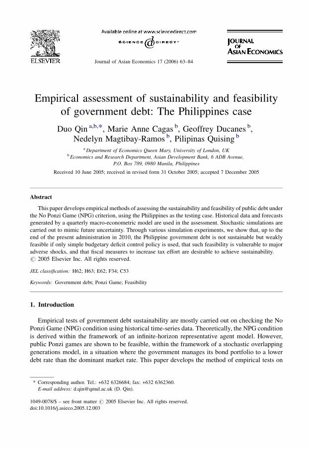
Fig. 1. Growth of GDP and ratio of fiscal balance to GDP. Source: National Statistical Coordination Board; Bureau of

Treasury.

from, its 2004 level. After enumerating and examining all the factors that will affect the future

value of this ratio, (i.e., existing debt-GDP ratio, the growth rate of output, the rate of inflation,

the rate of currency depreciation, the government’s primary surplus or deficit, domestic and

foreign interest rates, and the extent to which the government assumes the debts of failing

corporations or services contingent liabilities), the authors conclude that ‘‘sustainability

cannot be achieved without a radical change in observed trends.’’

Chronic deficits have marked the Philippine government’s fiscal position since the early years

of the country’s development.1 There was brief respite in the mid-1990s when the government’s

fiscal position improved enough to register a surplus of less than 1% for the period 1994–1997.

The occurrence of the Asian financial crisis, however, pushed the fiscal balance back to the

negative plane when it fell to�1.9% of GDP in 1998, and then plummeted to�5.2% in 2002. In

2004, the deficit stood at 3.9% of GDP (see Fig. 1).

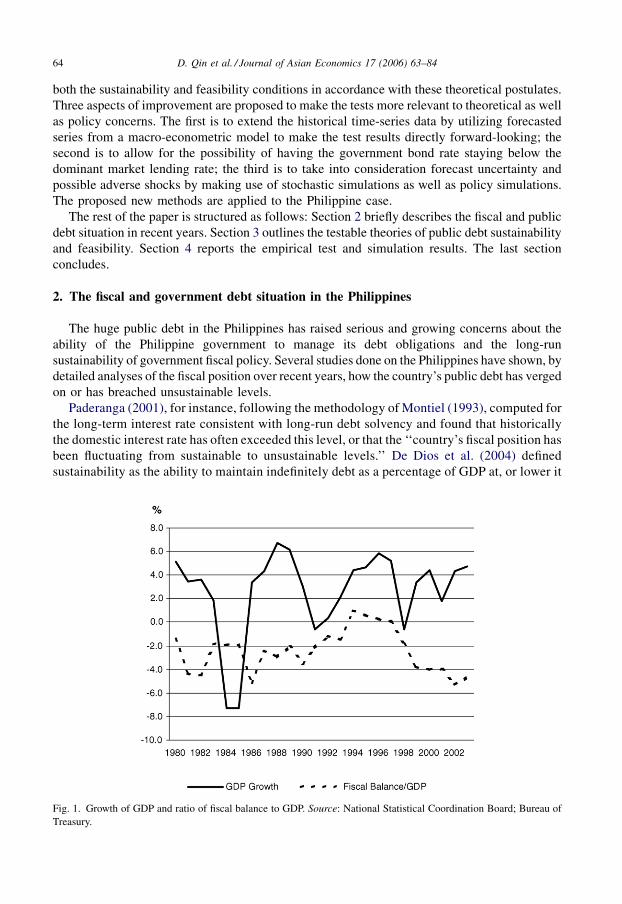
The deterioration of the fiscal balance is mostly due to shortfalls in government revenues,

especially tax revenues (which accounts for more than 85% of the total). The national

government’s revenue efforts have declined from a peak of 19.9% of GDP in 1994 to 14.5% of

GDP in 2004 (see Fig. 2). From its peak of about 17% in 1997, the tax effort has slid to 12.4%

in 2004. Government expenditures, on the other hand, have been fairly stable, averaging about

18% of GDP for the period 1980–2004. Its growth has been kept to a minimum and has been on

a downward trend since 2000. In particular, primary spending (i.e., national government

spending net of interest payments) has been reined in, with its share to GDP falling from 16.3%

D. Qin et al. / Journal of Asian Economics 17 (2006) 63–84 65

Fig. 2. Fiscal aggregates. Source: Bureau of Treasury.

1 In the 1960s, government was in deficit 8 out of the 10 years and fiscal deficit averaged about 1% of GDP for the

decade. In the 1970s it was in deficit 7 out of the 10 years and the fiscal deficit averaged about one-half of 1% of GDP. In

the 1980s the government was in deficit all 10 years and fiscal deficit averaged about 2.5% of GDP. See Manasan (1997,

2004) and Paderanga (1995, 2001) for a more extensive discussion of fiscal trends.

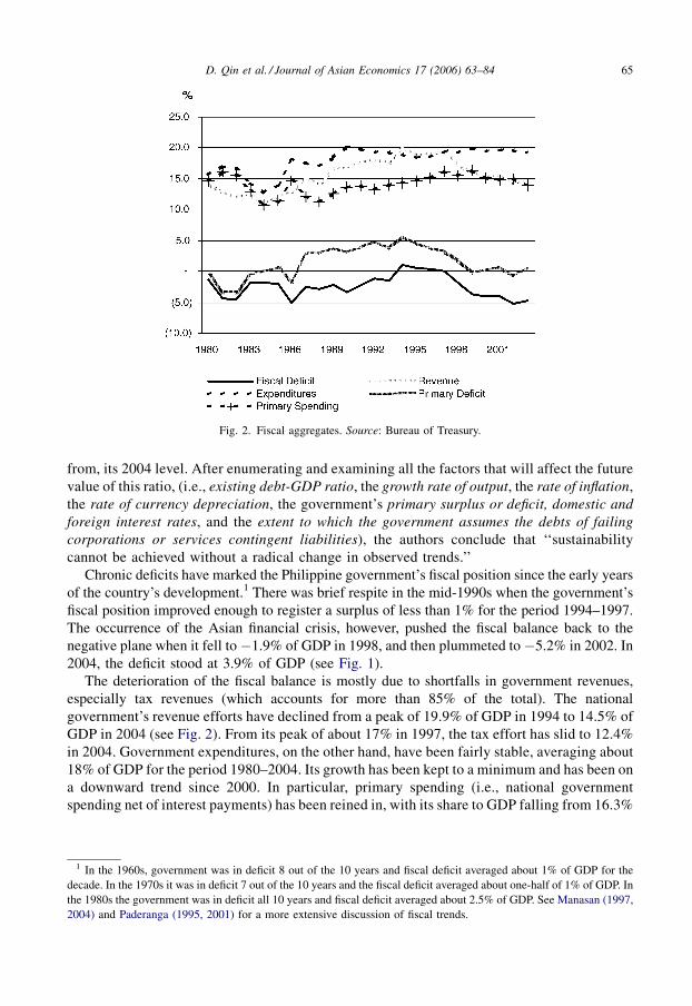
in 1999 to 13.0% in 2004. Capital expenditures have been reduced - after reaching its peak of

more than a quarter of total expenditures in the early 1980s, it is down to 14.9% in 2004.2 In

contrast, the amount spent for servicing of debt escalated. From an average of 4.6% in 1975–

1979, it went up to about 7% in 1980–1983, ballooned to almost 25% in 1984–1989 and has

averaged more than 25% in 2000–2004 (Fig. 3).

A major threat to the national government’s fiscal position is the large stock of national

government debt and the associated costs of servicing that debt. In the 1970s and 1980s, large

debt inflows were used to stimulate the economy and to provide a cushion against external shocks

that had often plagued the economy in the early years of its development. Then in the 1990s it

also became a means to service the liabilities of ailing government agencies. By this time,

domestic resources have become a significant part of Philippine public debt reflecting the

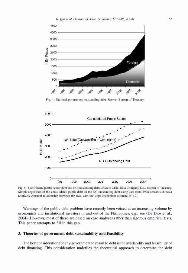
government’s struggle to service its foreign debt while incurring fiscal deficits (Fig. 4). From a

peak of 95.4 billion in 1994, primary balance (i.e., total revenues less non-debt expenditures)

went into deficit in 2002 ( 24.9 billion) before registering a surplus of 74.2 billion in 2004.

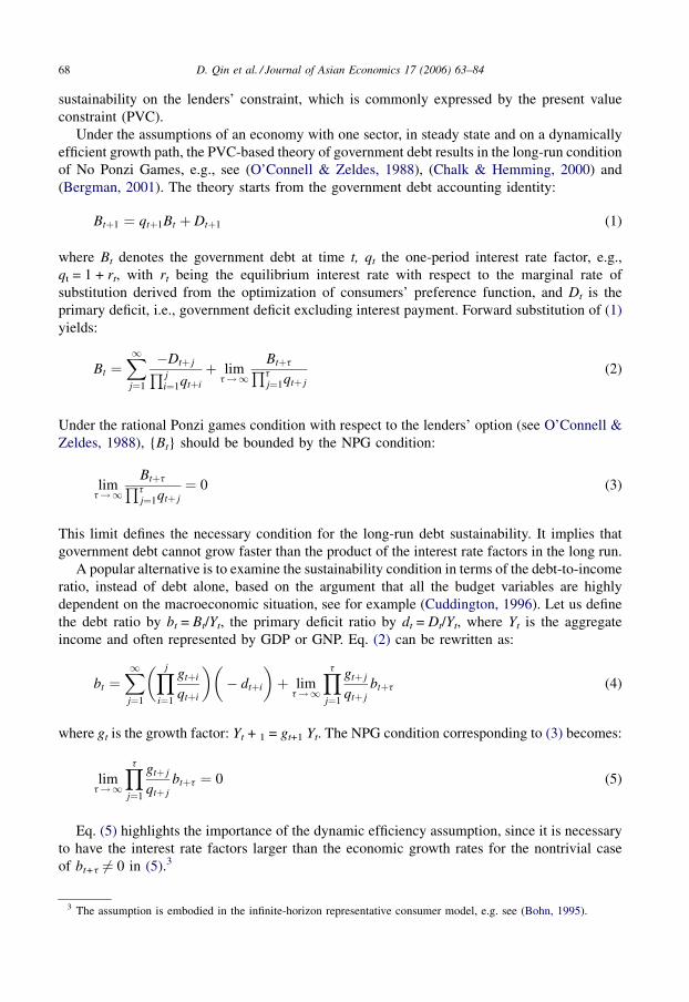
The national government’s total outstanding debt stood at 3.81 trillion (which is 79% of

GDP) at the end of 2004. Including contingent liabilities, this would amount to about 4.6 trillion

(or 96.3% of GDP). The consolidated public sector debt is much higher at 5.3 trillion—a

whooping 110% of GDP. All three are on an upward trend (Fig. 5).

The growth of public debt has been very high, averaging above 15% during 1999–2004. NG

debt has been growing at a higher rate for the same period, with the increase largely attributed

to the continuing national government deficits. However, an equally sizeable amount (about

37%) of the increase in debt is due to non-budgetary items and assumed liabilities of

government corporations, see Fig. 5, underscoring the continuous practice of condoning

inefficiency and irresponsibility of government-owned and controlled corporations.


Fig. 3. National government (NG) expenditures 2004. Source: Department of Budget and Management.

2 Of note is the fact that infrastructure spending of the national government has remained repressed and has not

exceeded 2% of GDP. Indeed, the brunt of fiscal adjustment has primarily been absorbed by infrastructure and other

development spending—expenditures developing countries like the Philippines badly need.

Warnings of the public debt problem have recently been voiced at an increasing volume by

economists and institutional investors in and out of the Philippines, e.g., see (De Dios et al.,

2004). However, most of these are based on case analyses rather than rigorous empirical tests.

This paper attempts to fill in this gap.

3. Theories of government debt sustainability and feasibility

The key consideration for any government to resort to debt is the availability and feasibility of

debt financing. This consideration underlies the theoretical approach to determine the debt


Fig. 4. National government outstanding debt. Source: Bureau of Treasury.

Fig. 5. Consolidate public sector debt and NG outstanding debt. Source: CEIC Data Company Ltd., Bureau of Treasury.

Simple regression of the consolidated public debt on the NG outstanding debt using data from 1998 onwards shows a

relatively constant relationship between the two, with the slope coefficient estimate of 1.2.

sustainability on the lenders’ constraint, which is commonly expressed by the present value

constraint (PVC).

Under the assumptions of an economy with one sector, in steady state and on a dynamically

efficient growth path, the PVC-based theory of government debt results in the long-run condition

of No Ponzi Games, e.g., see (O’Connell & Zeldes, 1988), (Chalk & Hemming, 2000) and

(Bergman, 2001). The theory starts from the government debt accounting identity:

Btþ1 ¼ qtþ1Bt þ Dtþ1 (1)

where Bt denotes the government debt at time t, qt the one-period interest rate factor, e.g.,

qt = 1 + rt, with rt being the equilibrium interest rate with respect to the marginal rate of

substitution derived from the optimization of consumers’ preference function, and Dt is the

primary deficit, i.e., government deficit excluding interest payment. Forward substitution of (1)

yields:

Bt ¼X1j¼1

�Dtþ jQ ji¼1qtþi

þ limt!1

BtþtQtj¼1qtþ j

(2)

Under the rational Ponzi games condition with respect to the lenders’ option (see O’Connell &

Zeldes, 1988), {Bt} should be bounded by the NPG condition:

limt!1

BtþtQtj¼1qtþ j

¼ 0 (3)

This limit defines the necessary condition for the long-run debt sustainability. It implies that

government debt cannot grow faster than the product of the interest rate factors in the long run.

A popular alternative is to examine the sustainability condition in terms of the debt-to-income

ratio, instead of debt alone, based on the argument that all the budget variables are highly

dependent on the macroeconomic situation, see for example (Cuddington, 1996). Let us define

the debt ratio by bt = Bt/Yt, the primary deficit ratio by dt = Dt/Yt, where Yt is the aggregate

income and often represented by GDP or GNP. Eq. (2) can be rewritten as:

bt ¼X1j¼1

�Yj

i¼1

gtþi

qtþi

�� dtþi

�þ lim

t!1

Ytj¼1

gtþ j

qtþ jbtþt (4)

where gt is the growth factor: Yt + 1 = gt+1 Yt. The NPG condition corresponding to (3) becomes:

limt!1

Ytj¼1

gtþ j

qtþ jbtþt ¼ 0 (5)

Eq. (5) highlights the importance of the dynamic efficiency assumption, since it is necessary

to have the interest rate factors larger than the economic growth rates for the nontrivial case

of bt+t 6¼ 0 in (5).3


3 The assumption is embodied in the infinite-horizon representative consumer model, e.g. see (Bohn, 1995).

Empirical tests of the debt sustainability conditions (3) or (5) entail knowledge of the time-

series properties of the variables in these equations, since these conditions require us to infer the

asymptotic properties of the limit functions from finite data samples. In particular, it is crucial to

know the time-series properties of the debt or debt ratio series, as the interest rate and the

economic growth rate are normally expected to be either stationary or non-trended randomwalk.4

Following (Bergman, 2001), we assume that the government debt be generated by a first-order

autoregressive, i.e., AR(1), process: 5

Bt ¼ a0 þ a1Bt�1 þ et ¼Xt�1

k¼0

a0ak1 þ at

1B0 þXt�1

k¼0

ak1et�k (6)

where et is a zero-mean stationary process. When a1 < 1, the NPG condition (3) is satisfied.

When the debt series is nonstationary, i.e., a1 � 1, the NPG condition (3) can be examined by

combining it with (6):

limt!1

BtþtQtj¼1qtþ j

¼ limt!1

�1Qt

j¼1qtþ j

�� Xtþt�1

k¼0

a0ak1 þ atþt

1 B0 þXtþt�1

k¼0

ak1etþt�k

�(7)

The NPG condition now becomes:

limt!1

Ptk¼0a0a

k1Qt

j¼1qtþ j¼ 0; lim

t!1

at1Qt

j¼1qtþ j¼ 0 (8)

Condition (8) requires that the degree of explosiveness in the roots of the debt series be no

larger than what the compounding interest rates could dampen out in the long run.

The same approach applies if empirical tests are based on the debt ratio. Starting from an

AR(1) process:

bt ¼ b0 þ b1bt�1 þ nt (9)

where nt is a zero-mean stationary process, and combining it with (5):

limt!1

Ytj¼1

gtþ j

qtþ jbtþt ¼ lim

t!1

�Ytj¼1

gtþ j

qtþ j

�� Xtþt�1

k¼0

b0bk1 þ btþt

1 b0 þXtþt�1

k¼0

bk1ntþt�k

�; (10)

we obtain the following convergence conditions:

limt!1

Ytj¼1

gtþ j

qtþ j

Xtk¼0

b0bk1 ¼ 0; lim

t!1

Ytj¼1

gtþ j

qtþ jbt1 ¼ 0 (11)

It is a widely known fact that government bonds normally enjoy significantly lower interest rates

than the market equilibrium rates. Moreover, many governments utilize the bond market to

reduce their debt interest payments by issuing bonds of different maturities to roll over

government debt, e.g., see (Bohn, 1995, 1998). As a result, the aggregate interest rate of the


4 A number of empirical tests are built on the time-series relationship between the fiscal deficit and the debt series, see

e.g. (Quintos, 1995; Bohn, 1998). However, this approach is not applicable here since there is an off-budget deficit

component in the Philippine government debt.5 This is a testable assumption. The results below can be extended to an AR(n) process when n > 1.

government bond portfolio is normally lower than the growth rate of the economy, making the

simple NPG scheme (5) implausible, see e.g. (Blanchard &Weil, 2001). Under this situation, the

issue then becomes to what extent the government can violate the present value budget constraint

and make it feasible to play debt Ponzi games.

In a recent paper, Barbie, Hagedorn, and Kaul (2004) investigate this issue by means of the

stochastic overlapping generations model. They establish the necessary and sufficient conditions

of the feasibility of government debt Ponzi games under a scenario where the government utilizes

rollover bond issuance strategies.6 Their conditions essentially boil down to the non-divergence

of the ratio of the aggregate interest rate of the public bond portfolio to the economic growth rate

under all kinds of stochastic shocks:

limt!1

Ytj¼1

qbðzÞtþ j

gðzÞtþ j

<1 ðnecessary conditionÞ (12)

X1j¼1

�Ytj¼1

qbðzÞtþ j

gðzÞtþ j

�j

� f<1 ðnecessary and sufficient conditionÞ (13)

where qb denotes aggregate interest rate factor of the government bond portfolio, z denotes the

state of random shocks and f a finite positive bound representing the credit constraint faced

by the government. Conditions (12) and (13) show that government Ponzi games would not

be possible unless the government could obtain debt finance at a lower interest rate than

the average economic growth rate in the long run. Barbie et al. (2004) refer to the ratio, qb/g,

as the real interest rate of debt payment, and to f as setting a fixed upper bound for the debt

ratio. The latter is not difficult to see if we assume (5) converges to a positive number instead

of zero when the interest rate is the lower-than market bond rate, i.e.:

limt!1

Ytj¼1

gtþ j

qbtþ j

btþt ¼ l> 0) limt!1

btþt ¼ l limt!1

Ytj¼1

qbtþ j

gtþ j;

provided that limt!1

Ytj¼1

gtþ j

qbtþ j

6¼ 0:

(14)

4. Empirical tests of government debt sustainability and feasibility

In this section, empirical tests are conducted on the Philippine national government (NG)

outstanding debt, using quarterly data series starting from 1990 (see the Appendix A for detailed

data description and sources). Notice from Fig. 5 that this debt series is significantly smaller than

the consolidated public sector debt. The gap, often referred to as sub-sovereign debt, is mainly

due to the liabilities of government-owned and controlled corporations and is not considered in

the standard NPG conditions, e.g., see Lebow (2004). Here, we follow suit in spite of the sizeable

sub-sovereign debt in the Philippines. The main reason is that data on sub-sovereign debt is

available only at the annual frequency. However, a look at recent historical data shows that

consolidated public debt has been roughly stable at about 1.2 times the NG debt (see the footnote


6 Notice that the condition for feasibility is weaker than that for sustainability, see (Barbie, Hagedorn, & Kaul, 2001).

in Fig. 5). If sub-sovereign debt remains proportional to the sovereign debt, the conclusions that

we draw from the empirical tests on the NG debt - which depends on the movement of the series -

should be also applicable to the consolidated public debt.

Almost all the empirical tests of government debt sustainability in the academic literature

have been carried out on the basis of the time-series properties of the historical debt series, e.g.,

see (Bohn, 1998). However, a major weakness of these tests is that the results based on past data

may not be directly projected into the future, where all the PVC theories are really focused on.

This can be especially worrisome considering that the dynamics of the government debt tends to

be highly susceptible to the macroeconomic environment in a small and open economy like the

Philippines. Noticeably, the IMF assessments of fiscal sustainability are based on projections of

the economic variables in (2) or (4) using the latest macroeconomic data, see e.g. (Chalk &

Hemming, 2000). Here, we adopt the same approach and use a quarterly macro-econometric

model of the Philippines to produce the projection. Specifically, we conduct the tests by

combining historical data, presently covering 1993Q1–2004Q2 in quarterly frequency, with

forecasted future series from the model, which was recently built by the Asian Development

Bank (we refer to this model as the ADB Philippine model thereafter).

The ADB Philippine model contains over 80 variables and is estimated using the data sample

mainly from 1990Q1 to 2003Q4, although some data series are shorter, e.g., the government

fiscal account series, including the debt series to be used in our tests, start from 1993Q1. All the

behavioral equations of the model are econometrically estimated following the so-called LSE

dynamic-specification approach, see e.g. (Hendry, 1995, 2002), though strong but data

permissible restrictions on certain long-run parameters are sometimes imposed for theoretical

coherence. Parameter estimates are ensured to be robust through recursive estimations and the

minimal use of dummy variables. Within sample, the model exhibits good forecasting ability as

gauged by conventional measures such as the root mean square percentage error and the mean

absolute percentage error. Out of sample, the model is judged to give good forecasts based on

stochastic simulations that show relatively narrow bands for the forecasts. Moreover, in actual

use since the mid 2004, the model forecasts have turned out to be quite accurate so far,

particularly those of major macroeconomic variables such as GDP growth and inflation. Below,

we give a brief description of the equations in the fiscal block of the model, a block that has been

especially designed to tackle the government debt issue, see (Ducanes, Cagas, Qin, Quising, &

Magtibay-Ramos, 2005) and (Cagas, Ducanes, Magtibay-Ramos, Qin, & Quising, 2006) for a

more detailed description of the entire model.

Government total revenue is modeled as a simple linear function of the government tax

revenue. Government tax revenue in turn is modeled in the long run as linear with respect to GNP

while also depending on the tax rate, and in the short run as depending on changes in GNP.

Meanwhile, government total expenditure is divided into non-interest expenditure and interest

payment on debt. Non-interest expenditure is formulated in the long run as linear with respect to

government total revenue while also being affected by the debt-to-GDP ratio negatively and the

unemployment rate positively and, in the short run, by changes in government total revenue and

the unemployment rate. Interest payment, on the other hand, is modeled as a fraction of total debt

and depends on the treasury bill rate and the exchange rate.

Because a significant portion of central government debt is due to non-deficit financing factors

such as the assumption of the debts incurred by state-owned enterprises, debt is modeled as a

behavioral equation rather than an identity. Domestic and foreign debts are modeled separately.

Change in government domestic debt is formulated in the long run as linear with respect to the

government deficit. In the short run, the acceleration of domestic debt is modeled to depend on


changes in the government deficit and the 91-day t-bill rate. Change in government foreign debt is

modeled in the long run as likewise linear with respect to the government deficit while also

depending on the exchange rate. In the short run, the acceleration of foreign debt is modeled to

depend on changes in the US lending rate, the interest differential between domestic and US

lending rates, and the exchange rate.

The forecast period in our tests is 2004Q3–2014Q4. Forecast values of some exogenous

variables are partly based on forecasts from the OECD Economic Outlook and Oxford Economic

Forecasting World Model; otherwise, the forecasts of an exogenous variable are extrapolated

from its present time path. During the forecast period, a large number of stochastic simulations

are computed using the bootstrap method for shock generation.7 This method enables us to

empirically mimic the z component of Eqs. (12) and (13) in accordance with the random patterns


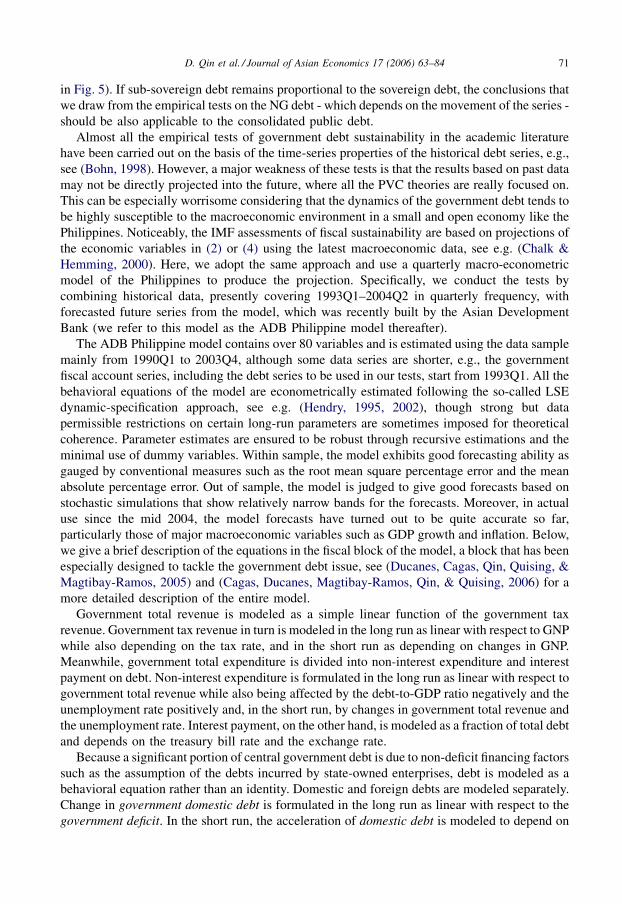
Fig. 6. Debt, Bt, and debt/GDP ratio, bt: historical data plus forecasts by stochastic simulations. Note: The solid lines are

the mean data series; the dotted lines are the upper and the lower series forming approximately 95% confidence interval.

Table 1

Unit root tests by augmented Dicky–Fuller (ADF) test

Augmented lags ADF-test b for Yt�1 t-value of

longest lag

Significance level

of longest lag

Debt series

3 2.03 1.01 �0.52 0.60

2 2.00 1.01 4.49 0.00

1 4.78 1.02 �1.55 0.12

0 4.52 1.01

Debt ratio series

3 �0.74 0.98 0.91 0.37

2 �0.66 0.99 �1.83 0.07

1 �0.86 0.98 �0.06 0.95

0 �0.88 0.98

The null hypothesis is b = 0. The critical values of ADF tests are: �2.90 at 5% and �3.51 at 1%. The sample covers

1994Q1–2014Q4. Seasonal dummies are added in the debt ratio test, as the series exhibits significant seasonal feature

inherent from GDP.

7 The method randomly draws shocks from single equation residuals over a specified historical sample period and adds

them to each forecast period. For more details, see (Pierse, 2001).

of the ADB Philippine model residuals. Quantiles are calculated from the large set (400 in our

experiments) of the simulation results to illustrate the distribution of the stochastic forecasts. In

particular, values at 2 and 97% quantiles are used as the approximate 95% confidence band of the

simulation mean values. Below, we refer to the data series of the simulation mean values as the

‘mean’ data series and the other two as the ’upper’ and ’lower’ data series respectively. Fig. 6

shows the debt and debt ratio series with these forecasting bands.

Let us first examine the simple time-series properties of the government debt and debt/GDP

ratio series, respectively. As shown from the unit-root test results in Table 1, both series exhibit

strong non-stationary properties, with the debt series showing certain explosive tendency. The

test results are also reflected in the ensuing regression analysis. We start by running an AR(4)

model for the debt and debt ratio series respectively in order to test the assumption of AR(1) in

Eqs. (6) and (9). As visible from Table 2, the assumed AR(1) process is accepted for the debt ratio


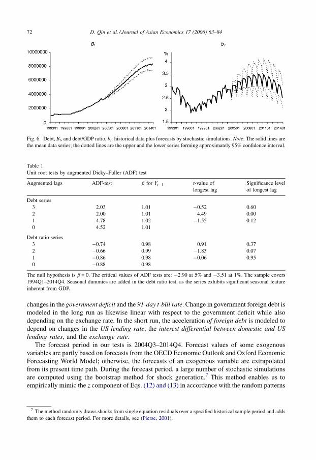
Fig. 7. Recursive estimates of b1 in Equation (9).Note: The central black curve is the recursive b1 using the mean bt series

shown in Fig. 6; the two grey curves on each side are the recursive b1 using respectively the upper and lower series of btshown in Fig. 6. The lower dotted line is the lower b1 curve minus its standard deviations multiplied by two whereas the

upper dotted line is the upper b1 curve plus its standard deviations multiplied by two. The two dotted lines could be seen

roughly as the 95% confidence intervals of b1 covering both estimation uncertainty and forecast uncertainly.

Table 2

AR(4) Estimations for the median series of debt and debt ratio

Coefficient Lag 1 Lag 2 Lag 3 Lag 4 Intercept

Full sample: 1994Q1–2014Q4

Debt 0.9410 (0.1087)* 0.5521 (0.1485)* �0.5482 (0.1516)* 0.0630 (0.1209) 26180 (13810)

Debt ratio 0.9950 (0.1102)* �0.2063 (0.1511) 0.2951 (0.1514) �0.1004 (0.1102) 0.0474 (0.0632)

Sub-sample: 1994Q1–2009Q4

Debt 1.0037 (0.1243)* 0.2291 (0.1783) �0.1526 (0.1807) �0.0629 (0.1274) 8866(13270)

Debt ratio 0.9875 (0.1274)* �0.0895 (0.1745) 0.1760 (0.1749) �0.0874 (0.1745) 0.0401 (0.0776)

Historical data: 1994Q1 to 2004Q2

Debt 0.9432 (0.1544)* 0.0138(0.2053) 0.0968 (0.2064) 0.0117 (0.1624) �47302(25420)

Debt ratio 1.0462(0.157)* �0.0173 (0.225) 0.1146 (0.2272) �0.1995 (0.1582) 0.1385 (0.1339)

The statistics in brackets are standard errors. Those marked by (*) are significant at 5%. Seasonal dummies are added in

the AR(4) model for the debt ratio.

series in both the full-sample and sub-sample estimations whereas the debt process is captured by

an AR(3) in the full-sample estimation and by an AR(1) only in the sub-sample estimations.

Moreover, the one-lag coefficient estimates for the debt ratio exhibit stronger time invariance

than those for the debt series, conforming to what was expected in the previous section.


Fig. 8. Interest rates. Note: TB rate denotes 91-days treasury bill rate. The solid lines are the mean data series; the dotted

lines are the upper and the lower series forming approximately 95% confidence interval.

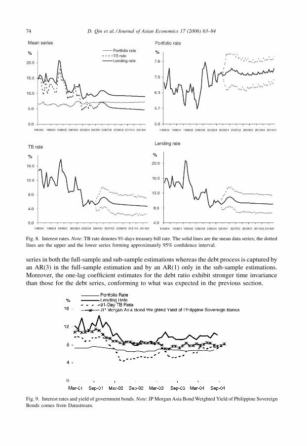
Fig. 9. Interest rates and yield of government bonds.Note: JP Morgan Asia BondWeighted Yield of Philippine Sovereign

Bonds comes from Datastream.

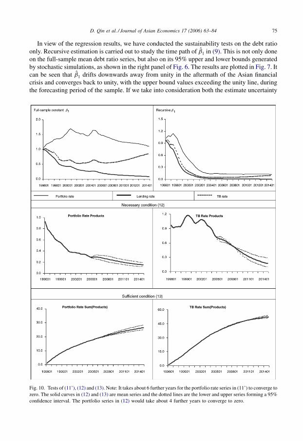
In view of the regression results, we have conducted the sustainability tests on the debt ratio

only. Recursive estimation is carried out to study the time path of b1 in (9). This is not only done

on the full-sample mean debt ratio series, but also on its 95% upper and lower bounds generated

by stochastic simulations, as shown in the right panel of Fig. 6. The results are plotted in Fig. 7. It

can be seen that b1 drifts downwards away from unity in the aftermath of the Asian financial

crisis and converges back to unity, with the upper bound values exceeding the unity line, during

the forecasting period of the sample. If we take into consideration both the estimate uncertainty


Fig. 10. Tests of (11’), (12) and (13). Note: It takes about 6 further years for the portfolio rate series in (11’) to converge to

zero. The solid curves in (12) and (13) are mean series and the dotted lines are the lower and upper series forming a 95%

confidence interval. The portfolio series in (12) would take about 4 further years to converge to zero.

and the forecast uncertainty, it is apparent that the debt ratio exhibits a unit-root process, as unity

is well within the 95% confidence interval through the entire sample. This implies that the debt

ratio is unlikely to play the dampening role desired in fulfilling the NPG condition, leaving

sustainability crucially to the future time paths of economic growth rates and interest rates.

Considering the finite-sample uncertainty in b1, two versions of condition (11) are tested, one

using the full sample estimate b1 and the other the recursive b1;tþ j:�Ytj¼1

gtþ j

qtþ jbt

1

�;

�Ytj¼1

gtþ j

qtþ j

Ytj¼1

b1;tþ j

�(11’)

to keep the paper short, only the b1 based on the mean debt ratio series are used for the tests. The

condition relating to the intercept term is disregarded here because its estimates are insignificant,

as shown in Table 2.

In the NPG theories, government bonds are assumed to bear the same rate as the equilibrium

interest rate. However, this assumption seldom holds in reality. Thus, in order to examine the

different effects of interest rates, we consider three rates: market lending rate, 91-day Treasury

bill (TB) rate, and government debt portfolio rate derived from the government debt interest

payment and the debt series. As seen from Fig. 8, the government rates are remarkably lower

than the market rate. More interestingly, the derived portfolio rate is far smoother than the TB

rate, possibly reflecting government efforts in debt portfolio management to minimize and

stabilize the debt cost payment. To check whether the chosen rates represent adequately the

market rates for the government bonds, Fig. 9 plots these rates together with the JPMorgan bond

yield of the weighted Philippine sovereign bonds for the period of 2000Q1–2004Q2.

Discernibly, the 91-day TB rate and the portfolio rate are a bit lower than the JP Morgan bond

yield while the lending rate is higher. This suggests that the test results from the three rates

should provide us with a fairly good confidence region.

Three pairs of the series in (11’) are calculated, each using one of the three interest rates. The

results are plotted in Fig. 10. Noticeably, the results using the full-sample coefficient estimate

show significantly higher values than those using the recursive results. This is due to the fact that

b1 exceeds its sub-sample estimates for over one third of the sample period, as shown in Fig. 7.

However, the full-sample b1 should be relatively reliable for out-of-sample inference based on


Fig. 11. Assumed exchange rate devaluation (peso/US$).

the recursive results as it converges to a highly constant value with the sample size. Notice that

the lending rate appears to provide the only case where the NPG condition is likely to be satisfied

in the infinite future, as it gradually decreases with time. The series based on the portfolio rate

also appears to be converging very slowly and is estimated to be approximately zero around 2020,

indicating that government Ponzi game is present during the current regime.8


Fig. 12. Testsof (11’), (12) and (13)under exchangerateshocksimulation.Note: In this simulation, theexchange ratedevalues

by 11, 14, 10 and 5% for the consecutive four quarters starting from 2005Q4, recovers by 5% in 2006Q4 and drops by 2% in

2007Q1, and stays constant afterwards. Convergence to zero is unachievable for the portfolio rate series in (11’) and (12).

8 The next election year is 2010.

To directly assess the feasibility of the Ponzi game, we calculate the test series of (12) and (13)

using the portfolio rate and the TB rate respectively, and plot them in Fig. 10. The results show

that only the necessary condition is satisfied up to 2010, not the sufficient condition. This

indicates the feasibility of the debt Ponzi game played by the government to be near the

borderline of becoming infeasible for the foreseeable future. Nevertheless, the sufficient

condition (13) is likely to hold for the infinite future as both test series under (12) show a

downward trend towards zero. Noticeably, the series for the necessary condition using the

portfolio rate shows a visibly slower converging speed than that using the TB rate, implying that

the government bond portfolio faces a tighter credit constraint than short-term bills. This suggests

the increasing risk that investors attach to the government bonds of longer terms.

Indeed, practical concerns over the future uncertainty of the debt situation are asymmetric,

i.e., investors are far more watchful of those uncertain situations when the sustainability or

feasibility of government debt is at risk of being violated than vice versa. The worry is

warranted by a number of government debt default crises triggered by adverse shocks in small

and open economies with weak governments, such as Argentina and Brazil.9 Since the

feasibility test results in Fig. 10 indicate that the present debt situation in the Philippines is

about marginally feasible, we run a model simulation to examine how much an adverse shock

would worsen the government debt situation. The simulation assumes the adverse shock to be a

currency crisis occurring in 2005Q4–2006Q4, with the peso-dollar exchange rate devaluing

40% in total (see Fig. 11).10

Both the sustainability test (11’) and the feasibility tests (12) and (13) are recalculated using

the simulation results for the forecasting sub-sample, see Fig. 12. In comparison with Fig. 10, the

sustainability results (11’) are now in a visibly worse state, especially with the disappearance


Fig. 13. Fiscal impact of the first simulation: budget deficit and GDP growth.

9 Calvo, Izquierdo, and Talvi (2003) demonstrate how a mismatch in the public debt composition led to a crisis in

Argentina triggered by its currency devaluation shock; Razin and Sadka (2002) show how a forthcoming election in

Brazil, which indicates expected regime change, could trigger a debt crisis even though the debt ratio is relatively low and

the fundamentals are sound.10 The exchange rate is exogenous in the Philippine model. Since the model also assumes the world trade demand as

exogenous, the simulation does not reflect the possible reactions of this variable to the devaluation shocks.

of the downward trend in the series based on the portfolio rate and the lending rate; the test results

using the portfolio rate no longer hold for either (11’) or (12), illustrating that the currently

feasible state of the government debt is indeed fragile and highly susceptible to adverse external

shocks.

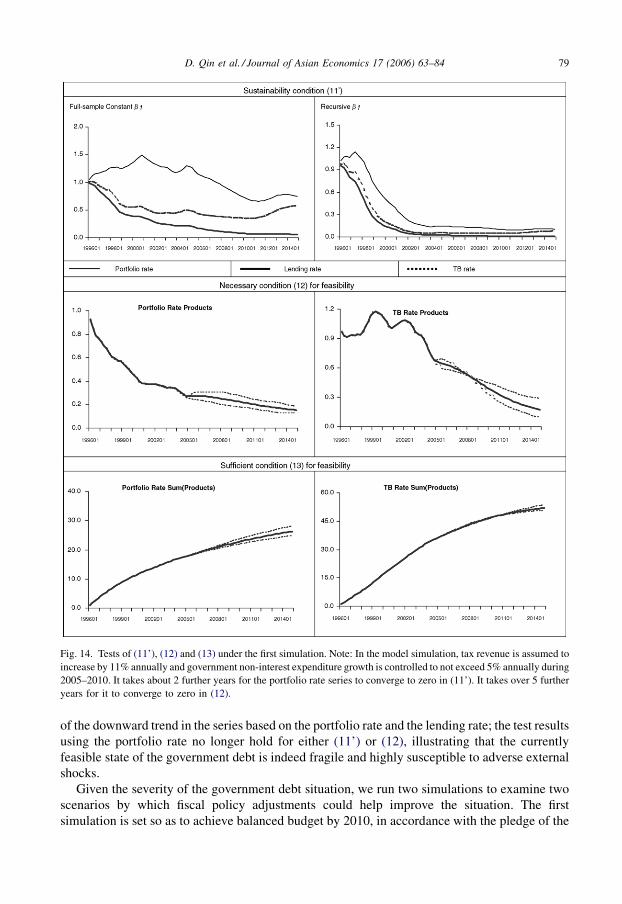
Given the severity of the government debt situation, we run two simulations to examine two

scenarios by which fiscal policy adjustments could help improve the situation. The first

simulation is set so as to achieve balanced budget by 2010, in accordance with the pledge of the


Fig. 14. Tests of (11’), (12) and (13) under the first simulation. Note: In the model simulation, tax revenue is assumed to

increase by 11% annually and government non-interest expenditure growth is controlled to not exceed 5% annually during

2005–2010. It takes about 2 further years for the portfolio rate series to converge to zero in (11’). It takes over 5 further

years for it to converge to zero in (12).

current government. Among the various schemes of curbing fiscal expenditure and raising tax

revenue that we have experimented, we find that this is achievable by having the tax revenue

increase by 11% per annum11 together with a capped annual growth at 5% of the government

expenditure net of interest payment for 6 years, i.e., 2004Q4–2010Q4. The other simulation is


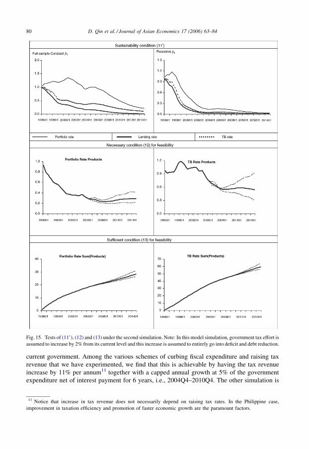
Fig. 15. Tests of (11’), (12) and (13) under the second simulation. Note: In this model simulation, government tax effort is

assumed to increase by 2% from its current level and this increase is assumed to entirely go into deficit and debt reduction.

11 Notice that increase in tax revenue does not necessarily depend on raising tax rates. In the Philippine case,

improvement in taxation efficiency and promotion of faster economic growth are the paramount factors.

more ambitious. It assumes an increase in tax income by 2% of GDP beginning 2005Q4 up to

the end of the simulation period.12 In addition, all additional revenues are assumed to go to

deficit and debt reduction and not to fund additional expenditures. This is admittedly a very

extreme case and is only done to get an indication of what it requires to achieve debt

sustainability in the country.

Fig. 13 shows the dynamic path of the budget deficit under the first simulation as compared

with that of the default simulation (the left panel), and the impact of this simulation on GDP

growth as well as interest rate (the right panel). Noticeably, the fiscal target leads to prompt deficit

deterioration post the target period and a persistent slowdown of the economy during the target

period, suggesting that such a target is highly likely to incur grave fiscal burden for the next

regime while depressing the overall economy during the present regime. This kind of policy

consequence is hardly surprising in view of the fact that the public sector in the Philippines is

already severely undersized, as described in Section 2, making any further squeeze untenable.

What is surprising are the simulation test results, which show no chance of achieving the

sustainability condition or the feasibility condition within the present regime (see Fig. 14), in

spite of the heavy policy cost. Our finding reveals the inadequacy of simple fiscal rules to control

the budget deficit if the aim is to achieve debt sustainability. Much more ambitious and

comprehensive policies are required.

The other simulation indicates that an increase in tax effort with the additional revenues

devoted entirely to deficit reduction will lead to debt sustainability during the simulation

period. In particular, a 2% increase in tax effort appears to offer the ‘‘best’’ case among all

assumed values in terms of attaining debt sustainability within the present regime. Fig. 15

shows sustainability and feasibility conditions for this scenario. Note that the recursive

sustainability graph already appears to show sustainability within the present regime, while

the full sample graph shows a quick movement towards sustainability towards the end of the

simulation period.

5. Conclusions

This paper develops empirical methods of assessing the sustainability and feasibility of

the government debt situation, using the Philippines as the testing case. The assessment is

based on the NPG criterion and mainly carried out on the debt-to-GDP ratio using both its

historical data and forecasts generated by a macro-econometric model of the Philippine

economy.

Our assessment shows that the government debt situation is unlikely to be sustainable as far as

the present regime is concerned. One key reason for the existing high government debt is the fact

that the government still enjoys lower bond rates than the market lending rates. In other words,

the Philippine government bonds are still perceived as having relatively low default risk. Our

assessment also shows that the Philippine government is playing a weakly feasible debt Ponzi

game. The debt strategy satisfies the necessary condition but fails the sufficiency condition for

feasibility up to 2014, although it might satisfy both conditions for the infinitely remote future.

These results indicate the vulnerability of the debt situation.


12 This may correspond to gains from the implementation of the Expanded Value Added Tax law (Revenue Regulation

No. 14-2005), or more efficient collection, since the efficiency has been very low. Simulations with slightly lower and

higher tax effort increases (from 1 to 3%) are also experimented but yield inferior results and are not presented here.

The vulnerability is further confirmed by our experiment of a shock simulation using the

Philippine model. We find that the government debt no longer satisfies the debt feasibility

condition under a hypothetical exchange rate crisis. This result shows that the government is

facing a high risk of running into a debt crisis in the event of a major adverse shock to the

economy.

Our findings provide strong support to the warnings about the critical government debt

situation and highlight the difficulty and the urgency of improving the government’s fiscal

position in the present Philippine economy. Indeed, our model simulation shows that the

simple fiscal policy of medium-term budget deficit control alone is inadequate for reversing

the unsustainable debt situation. In fact, further simulation experiments show that nothing

short of a significant increase in tax effort combined with severe fiscal discipline, in the sense

that all revenues are devoted entirely to deficit reduction, will lead to debt sustainability.

This underscores the importance of studying the dynamic interaction between proposed

corrective policies to control public debt and the underlying macroeconomic variables. Any

policy aimed at addressing the debt sustainability problem must take into account not just its

effect on debt but also its effect on other economic variables, such as interest rates and the

overall economic growth, which are themselves factors that determine debt sustainability.

What is highly needed are more comprehensive and well-coordinated policies aimed at

promoting sustained economic growth, increasing resilience to exogenous shocks as well as

improving debt management.

The results further point at the non-evadable responsibility that public debt creditors and

donors should take in helping the heavily debt-burdened country avoid a debt crisis. In particular,

large institutional creditors must review lending policies to ensure that their loans and

accompanying provisions are carefully based on the debt sustainability of the country concerned

as derived from its macroeconomic framework. If loan provisions are not based on market

perceived risk or if debt service can largely be covered by grants, aid, or debt relief, the

government will have little incentive to pursue sound macroeconomic policies and increase its

capacity to pay, see e.g. (IMF and IDA, 2004).

Acknowledgement

Thanks are due to W. Bikales, X-L. Liu, R. S. Ondrik and two anonymous referees for their

valuable comments.


Appendix A. Data description and sources

Data series Description Sourcea

91-day treasury bill rate (%) Weighted averages per annum CEIC Data Company Ltd., BSP,

ADB Philippine Model

Bond yield JP Morgan Asia Bond Weighted

Yield of Philippine Sovereign Bonds

Datastream

Fiscal deficit Revenue less expenditure BTr

Gross domestic product Current price (in million pesos) CEIC Data Company Ltd.,


Interest payments Current price (in million pesos) CEIC Data Company Ltd.,

BTr, ADB Philippine Model

References

Bergman, M. (2001). Testing government solvency and the No Ponzi Game condition. Applied Economics Letters, 8, 27–

29.

Barbie, M., Hagedorn, M., & Kaul, A. (2001). Government debt as insurance against macroeconomic risk. IZA

Discussion Papers, no. 481.

Barbie, M., Hagedorn, M., & Kaul, A. (2004). On the feasibility of debt Ponzi schemes—A bond portfolio approach:

Theory and some evidence. Universitat Karlsruhe WIOR Technische Reports 645.

Blanchard, O.-J., & Weil, P. (2001). Dynamic efficiency, the riskless rate, and debt Ponzi games under uncertainty. The

B.E. Journal in Macroeconomics 1(2) article 3.

Bohn, H. (1995). The sustainability of budget deficits in a stochastic economy. Journal of Money, Credit, and Banking, 27,

257–271.

Bohn, H. (1998). The behavior of U.S. public debt and deficits. Quarterly Journal of Economics, 113, 949–963.

Cagas, M. A., Ducanes, G., Magtibay-Ramos, N., Qin, D., & Quising, P. (2006). A small macroeconometric model of the

Philippines economy. Economic Modelling, 23. (This is a condensed and revised version of Ducanes et al. 2005).

Calvo, G. A., Izquierdo, A., & Talvi, E. (2003). Sudden stops, the real exchange rate and fiscal sustainability: Argentina’s

lessons. NBER Working Paper, no. 9828.

Chalk, N., & Hemming, R. (2000). Assessing fiscal sustainability in theory and practice. IMFWorking Paper, no. WP/00/

81.

Cuddington, J. T. (1996). Analyzing the sustainability of fiscal deficits in developing countries. Georgetown University

Working Paper, no. 97-01.

De Dios, E. S., Diokno, B. E., Esguerra, E. F., Fabella, R. V., Gochoco-Bautista, Ma. S., Medalla, et al. (2004). The

deepening crisis: the real score on deficits and the public debt. Discussion Paper DP2004-09, School of Economics,

University of Philippines.

Ducanes, G., Cagas, M. A., Qin, D., Quising, P., & Magtibay-Ramos, N. (2005). A small macroeconometric model of the

Philippines economy. ADB ERD Working Papers No. 62, http://www.adb.org/economics/erd_working_papers.asp.

Hendry, D. F. (1995). Dynamic economics. Oxford: Oxford University Press.

Hendry, D. F. (2002). Applied econometrics without sinning. Journal of Economic Surveys, 16, 591–604.

IMF and International Development Association. (2004). Debt Sustainability in Low-Income Countries–Proposal for an

Operational Framework and Policy Implications. At: http://www.imf.org/external/np/pdr/sustain/2004/020304.htm.

Lebow, D. E. (2004). Recent fiscal policy in selected industrial countries. BIS Working Papers 162.

Manasan, R. G. (1997). Fiscal adjustment in the context of growth and equity, 1986–1997. Discussion Paper Series 1998–

1911, Philippine Institute for Development Studies.


Lending rate (%) Weighted averages per annum. Annual rates are

averages of monthly rates. Monthly rates are

annual percentage equivalent of all commercial

banks’ actual monthly interest income on their

peso-denominated loans to the total outstanding

levels of their peso-denominated loans, bills

discounted, mortgage contract receivables

and restructured loans.

CEIC Data Company Ltd.,

BSP, ADB Philippine Model

National government

outstanding debt

Outstanding Domestic Debt + Outstanding

Foreign Debt, Current price (in million pesos)

CEIC Data Company Ltd., BTr,


Portfolio rate (%) Interest payments/National government

outstanding debt

CEIC Data Company Ltd., Btr,


Primary deficit Revenue less primary spending BTr

Primary spending Expenditure less interest payments BTr

a Actual data are sourced from CEIC and/or official sources. Forecast data are sourced from the ADB PhilippineModel.

Bureau of Treasury is abbreviated as BTr. Department of Budget and Management is abbreviated as DBM.

Appendix A (Continued )

Data series Description Sourcea

http://www.adb.org/economics/erd_working_papers.asp

http://www.imf.org/external/np/pdr/sustain/2004/020304.htm

Manasan, R. G. (2004). Fiscal reform agenda: getting ready for the bumpy ride ahead. Discussion Paper Series 2004–

2024, Philippine Institute for Development Studies.

Montiel, P. J. (1993). Fiscal aspects of developing country debt problems and debt and debt-service reduction operations.

World Bank Policy Research Working Paper No. 1073.

O’Connell, S. A., & Zeldes, S. P. (1988). Rational Ponzi games. International Economic Review, 29, 431–450.

Paderanga, Jr. C. (1995). Debt management in the Philippines, in Fabella, R. V., Sakai, H. (Eds.). Towards Sustained

Growth, Tokyo: Institute of Developing Economies.

Paderanga, Jr. C. (2001). Recent fiscal developments in the Philippines. School of Economics, University of Philippines.

Pierse, R. (2001). Winsolve Manual, Department of Economics, University of Surrey, UK.

Quintos, C. E. (1995). Sustainability of the deficit process with structural shifts. Journal of Business and Economic

Statistics, 13, 409–417.

Razin, A., & Sadka, E. (2002). A Brazilian debt-crises model. NBER. Working Paper, no. 9211.


empirical assessment of sustainability and feasibility of government debt: the philippines case

Documents