Emissivity profiles of AGN accretion discs

Dan Wilkins

X-ray BunClub – 21/05/2010

1.Concept of emissivity profiles

• Why should I care?

2.Determination from observed spectra

3.Test with XSPEC model

4.Theoretical predictions – ray tracing

Outline

2

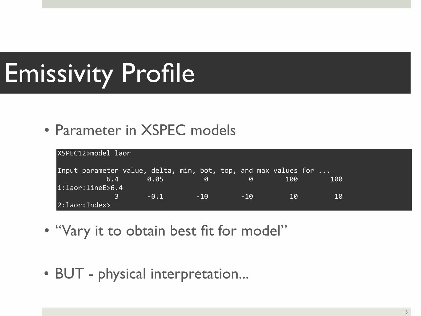
• Parameter in XSPEC models

• “Vary it to obtain best fit for model”

Emissivity Profile

3

XSPEC12>model laor

Input parameter value, delta, min, bot, top, and max values for ... 6.4 0.05 0 0 100 1001:laor:lineE>6.4 3 -­‐0.1 -­‐10 -­‐10 10 102:laor:Index>

• Parameter in XSPEC models

• “Vary it to obtain best fit for model”

Emissivity Profile

3

XSPEC12>model laor

Input parameter value, delta, min, bot, top, and max values for ... 6.4 0.05 0 0 100 1001:laor:lineE>6.4 3 -­‐0.1 -­‐10 -­‐10 10 102:laor:Index>

• BUT - physical interpretation...

‘Lamppost Model’

4

PLC

RDC

Hard X-ray source in coronaIC scattering of seed photons

Reflection from accretion disc. Atomic lines imprinted (reflionx)

• Reflected power per unit area from disc.

• Flux received at point on disc falls off with distance from X-ray source.

Emissivity Profile

5

• Reflected power per unit area from disc.

• Flux received at point on disc falls off with distance from X-ray source.

Emissivity Profile

5

F ∝ 1d2

=1

r2 + h2

d

h

• e.g. Euclidean space

r 1e-05

0.0001

0.001

0.01

0.1

1 10 100

• Depends on

• Source location/height

• Source extent

• Source/disc geometry

Emissivity Profile

6

• Depends on

• Source location/height

• Source extent

• Source/disc geometry

Emissivity Profile

6

• Constrain these from observed emissivity profiles?

ObservationsDetermining emissivity profiles from observed spectra...

• Typically assume (broken) power law emissivity profile.

• Can we determine emissivity profile from observed spectrum?

Emissivity Profiles from Spectra

8

105

11.

52

2.5

3

ratio

Energy (keV)

data/model

drw 5 May 2010 16:38

• Gravitational redshift

• Doppler shift

Broadened Emission Lines

9

F0(ν0) =

Ie(re,ν0

g)T (re, g)dgredre

I(re, ν) = δ(ν − νe)(re)

• Consider the line as sum of contributions from successive radii.

• Number of photons from each annulus

• A projected to observer.

Emissivity from Broad Lines

10

F0(ν0) =

T (re, g)redre(re)

N(r) ∝ A(r)(r)

• Model spectrum

• For K-line (3-10 keV), only dominant features are power law and reflected line.

• Power law, inclination and reflionx parameters from best fit to whole spectrum (Zoghbi+09).

• Fit for norm of each reflionx component.

• Divide by projected area of each annulus (transfer fn).

Emissivity from Broad Lines

11

powerlaw +

kdblur⊗ reflionx

10 3

0.01

norm

aliz

ed c

ount

s s

1 keV

1

data and folded model

105

0.8

1

1.2

ratio

Energy (keV)drw 20 May 201

χ2 = 255.48

χ2 / NDoF = 1.1255

12

1H0707-495

• 3-5 keV• 3-10 keV

Results

13

α~7α~5.5

Lines above 20RG excluded from fit

α~3

• Miniutti+03

• Also Suebsuwong+06

Theoretical Prediction

14

• kdblur3 model

• As kdblur2

• Convolve with relativistic broad line profile but with twice-broken power law emissivity.

• Fit emissivity params.

Test Result with XSPEC Model

15

kdblur2 kdblur3

Index 1 4.82 7.72

R break 1 6.85RG 5.53RG

Index 2 2.09 8.46x10-5

R break 2 — 34.73RG

Index 3 — 3.38

χ2 287.52 272.39

χ2 / Ndof 1.11 1.07

3-10keV : powerlaw + kdblur⊗reflionx

16

Theoretical PredictionsRaytracing from the source to the accretion disc...

Building on work of Miniutti et al, Suebsuwong, Malzac et al in light of observations.

Develop a formalism for analysis...

xa + Γabcx

bxc = 0 gabxaxb = 0

• Light rays follow null geodesics in Kerr spacetime around (rotating) black hole.

Ray Tracing

18

ds2 = c2

1− 2µr

ρ2

dt2 +

4µacr sin2 θ

ρ2dtdϕ− ρ2

∆dr2 − ρ2dθ2

−

r2 + a2 +2µa2r sin2 θ

ρ2

sin2 θdϕ2

• Solve geodesic equations of the null (photon) geodesics...

Derivatives w.r.t. affine parameter, σ

Geodesic Equations

19

t =(r2 + a2 cos2 θ)(r2 + a2) + 2µa2r sin2 θ

k − 2µar

c h

r21 + a2 cos2 θ

r2 − 2µr

(r2 + a2) + 2µa2r sin2 θ

ϕ =2µacrk sin2 θ + (r2 + a2 cos2 θ − 2µr)h

(r2 + a2)(r2 + a2 cos2 θ − 2µr) sin2 θ + 2µa2r sin4 θ

θ2 =Q + (kca cos θ − h cot θ)(kca cos θ + h cot θ)

ρ4

r2 =∆ρ2

kc2t− hϕ− ρ2θ2 − 2

• So, given starting position of a photon and its constants of motion (initial direction), can propagate it.

• Affine parameter step variable as required:

(and similar in θ, ϕ – take the smallest, with limit).

Ray Tracing

20

r(σ + dσ) = r(σ) + rdσ

dσ = r−rH

r

τ

e(a) · e

(b) = η(a)(b)

• Source frame (flat)

• Photons at equal intervals in cos α and β

• Calculate h, Q from α and β (set k=1)

• Isotropic Point Source

• Equal power radiated into equal solid angle, in source frame.

The Source

21

dΩ = d(cos α)dβ

α

βei

e’i

θϕ

r

dΩ’

-10

-5

0

5

10

-10-5

0 5

10

0

2

4

6

8

10

"geodesic_x.dat"

• Schwarzschild Black Hole

• 6RG

22

-4

-2

0

2

4

-4-2 0 2 4

0

1

2

3

4

5

"geodesic_x.dat"

• Schwarzschild Black Hole

• 3RG

23

-10

-5

0

5

10

-10-5

0 5

10

0

2

4

6

8

10

"geodesic_x.dat"

• Kerr Black Hole, a = 0.998

• 6RG

24

Frame dragging

-4

-2

0

2

4

-4-2 0 2 4

0

1

2

3

4

5

"geodesic_x.dat"

• Kerr Black Hole, a = 0.998

• 3RG

25

-4

-2

0

2

4

-4-2 0 2 4

0

1

2

3

4

5

"geodesic_x.dat"

• Kerr Black Hole, a = 0.998

• 3RG, θ = π / 4

26

• Trace rays until they hit disc (or you get bored).

• Disc divided into radial bins.

• Count photons in bin.

• Emissivity – divide by area of annulus (rdr from definition of T!!!)

27

Emissivity Profiles from Ray Tracing

• Develop modular ray tracing code in Fortran 95 and C++.

• Re-use same library for ray tracing in any context.

• Parallelised

• For each point source, divide parameter space (cos α) equally between cluster nodes – each traces a set of rays.

• Master node collects and sums radial bins.

The Code

28

0.001

0.01

0.1

1

10

100

1000

10000

100000

1 10 100 1000

h = 3Rgh = 6Rg

h = 10Rgh = 20Rgh = 50Rg

Axial Source

29

50RG: α~2.7

3RG: α~3.4

50RG: α~3

0.001

0.01

0.1

1

10

100

1000

10000

100000

1 10 100 1000

a = 0a = 0.998

Axial Source – Schwarzschild

30

3RG

Lesser effect at greater source height.

Ring Source

31

Ring Source

31

Symmetry... equivalent to

0.001

0.01

0.1

1

10

100

1000

10000

100000

1 10 100 1000

th=pi/4, r=3Rgth=pi/4, r=6Rg

Ring Source

31

Symmetry... equivalent to

• Stationary sources do not reproduce steep emissivity profile in centre.

• Stationary ring source a bit unphysical!

• Moving source (e.g. ‘co-rotating’ with disc).

• Beaming of emission into ‘forward’ direction

• Increased emission onto inner disc.

• Coding this...

Moving Source

32

• Determination of emissivity profile from observed spectrum of 1H0707-495.

• Twice-broken power law.

• Fits with kdblur3 model.

• Beginnings of ray tracing simulations/theoretical profiles.

• Can reproduce index at large r, but not steep profile for inner disc.

Conclusions

33

Observation

• Higher resolution spectra – 1H0707 RGS data.

• Other sources - variation in profiles...

Theory

• Moving sources.

• Other source geometries

• Constraints on corona...?

Next Steps...

34