Emissions Modeling of Specific Highly Reactive Volatile Organic Compounds (HRVOC) in the Houston-Galveston-Brazoria Ozone Nonattainment Area

Ron Thomas, Jim Smith, Marvin Jones, Jim MacKay, John Jarvie Texas Commission on Environmental Quality (TCEQ), MC-164

P.O. Box 13087, Austin, TX 78711-3087 rthomas@tceq.state.tx.us

ABSTRACT

The 2006 Texas Air Quality Study (TexAQS II) confirmed many of the results from the 2000 Texas Air Quality Study (TexAQS 2000). Both of these studies rank among the most extensive and comprehensive studies of their kind undertaken to date. Chief among many important findings was the discovery of the role played by certain light olefins in the rapid, intense formation of ozone in the Houston-Galveston-Brazoria (HGB) ozone nonattainment area. Atmospheric concentrations of species such as ethylene and propylene were often found to be many times larger than could be explained by reported emissions inventories. Successfully modeling pollutant concentrations observed during the study necessitated adjustments to these reported emissions. As a consequence of these findings, in 2001, the Texas Natural Resource Conservation Commission (now Texas Commission on Environmental Quality) began developing regulations targeting specific highly-reactive VOCs (HRVOC). Adjusting the modeling inventories to account for unreported HRVOC emissions and later test-driving controls on emissions of these specific compounds presented a set of unique challenges to emissions modelers, since emission processing software typically is not designed to apply adjustments or controls to individual VOC species. This paper describes a set of procedures developed by TCEQ which allowed us to successfully adjust and control (in processing for the photochemical model) emissions of individual hydrocarbon species in the TexAQS 2000 modeling episode. This paper also provides an introduction to ongoing efforts to reconcile more recent inventories with ambient measurements made at twelve automatic gas chromatographs (auto-GCs) currently operating continuously in the HGB nonattainment area. INTRODUCTION Background and Motivation

The development of a strategy for reducing ozone in HGB is complicated by the many factors contributing to ozone formation in this area. A hot, sunny climate, a large urban population, a massive refining/petrochemical industry, and complex coastal meteorology all work together to make the area one of the worst in the nation for ground-level ozone, and at the same time one of the most challenging areas to model.

In December 2000, TCEQ adopted an HGB Attainment Demonstration Ozone SIP that included rules requiring a 90 percent nitrogen oxides (NOX) reduction from industrial sources within the HGB area. Shortly after the SIP revision was adopted, a group of Houston-area industrial companies challenged the December 2000 HGB SIP and some of the associated rules. Among other things, the group contended that the last 10 percent of the NOX reductions (i.e. requiring a 90% reduction instead of 80%) was not cost effective and that the ozone plan would fail because TCEQ did not account for volatile organic compound emissions associated with upset conditions. As part of a settlement agreement reached in June, 2001 TCEQ committed to investigate whether attainment could still be reached under alternatives to the 90 percent industrial NOX reduction strategy, specifically whether reductions to emissions of Highly-Reactive VOCs (HRVOCs) could be substituted for the last 10% of NOX reductions.

Complying with the Consent Order, TCEQ conducted a scientific evaluation based in large part

on aircraft data collected by the Texas 2000 Air Quality Study (TexAQS 2000). TexAQS 2000 was a comprehensive field study of ground-level ozone formation and transport conducted in August and September 2000 involving more than 40 research organizations and over 200 scientists, followed by several years of data analysis and interpretation. Probably the most important conclusion of TexAQS 2000 was that emissions of light olefins, particularly ethylene and propylene, were under-reported by as much as an order of magnitude or more.

To address the findings from TexAQS 2000 and fulfill obligations of the Consent Order, TCEQ adopted a SIP revision in December 2002 focused on replacing the final 10 percent of industrial NOX reductions with VOC controls. An analysis of automated gas chromatograph data1 revealed that four HRVOCs were frequently responsible for high reactivity days: ethylene, propylene, 1,3-butadiene, and butenes. The photochemical grid modeling results and analysis indicated that the HGB area could achieve the same air quality benefits seen with 90% NOX reductions with a combination of 80 percent industrial NOX emissions reductions together with sufficient reductions of HRVOCs. Consequently, these compounds were selected as the best candidates for highly reactive VOC (HRVOC) emission controls.

Before rules controlling emissions of HRVOCs could be developed, however, TCEQ would have to reconcile the reported emissions of these compounds with the conclusions of TexAQS 2000, which required a thorough understanding and accounting of the VOC species reported in the TCEQ 2000 EI. Unfortunately, the reported 2000 point source EI, as extracted for modeling from the TCEQ Point Source Database (PSDB) and its successor, the State of Texas Air Reporting System (STARS), contained a high percentage of “VOC-unclassified”; hence, the EI was far from fully-speciated. Modelers developed a procedure2 to fully-speciate a Texas EI for modeling.

Once a completely-speciated inventory was available, TCEQ developed a procedure for

reconciling the reported emissions of HRVOCs with aircraft measurements made during TexAQS 2000. This resulted in an increase of approximately 200 tons/day to modeled olefin emissions at industrial facilities in the 8-county HGB nonattainment area. This inventory adjustment produced a notable improvement in base-case photochemical model performance.

As part of the settlement (discussed above), the plaintiffs agreed to deploy and maintain eight automated gas chromatographs (auto GCs) in the HGB area beginning in 2005, measuring ambient concentrations of many hydrocarbon species. These monitors augmented the four TCEQ-operated auto GCs already in operation in the area. TCEQ staff is currently investigating a new technique for reconciling reported emissions with ambient concentrations using this extensive monitoring network. The technique combines modeling using the Industrial Source Complex (ISC) dispersion model with a technique designed to locate potential emission sources known as the Potential Source Contribution Function (PSCF). Some preliminary analysis using this technique will be discussed in a later section of this paper. Scope

In its most concise description, this paper is a compilation of the last seven years of TCEQ progress, centering on HRVOC development of EI, photochemical modeling, and rules that are intended to control HRVOC within the HGB nonattainment area. The scope of this paper is to guide the reader through the motivating factors, issues, and resolution of the development of TCEQ’s HRVOC emissions inventories, the modeling of the emissions adjustments, and the development of the HRVOC rules. Additionally, this paper briefly discusses the current work TCEQ is performing with regard to emissions

reconciliation of more recent modeling inventories with HRVOC and other VOC measured at several auto-GCs in HGB.

This paper will cover the flowing topics in individual sections of the body of the text:

• Reactivity • Speciation • Developing and Defining HRVOC Adjustment • Modeling the Adjustment • HRVOC Controls • HRVOC Rules • Recent Developments in Emissions Reconciliation

Highlights of Results

Relying on results of the TexAQS 2000 field campaign, TCEQ was able to improve the performance of the photochemical model in HGB by adjusting the amount of modeled HRVOC emissions available for rapid ozone formation in 2000. A key component of this process involved developing a process to fully speciate the reported emissions of industrial sources. Using the adjusted inventory, TCEQ was able to demonstrate that 80 percent NOX reduction combined with overall 36 percent HRVOC reductions is equivalent to the 90 percent industrial NOX reduction. To achieve the necessary HRVOC reductions, TCEQ developed a dual approach: (1) address variable short-term emissions through a 1200 lb/hour, not-to-exceed, emission limit, and (2) address steady-state and routine emissions through an annual cap. The paper concludes with a preview of current work TCEQ is undertaking to reconcile monitored ambient emissions with the reported inventory. DISCUSSION Reactivity

As modelers and atmospheric scientists, we ask the question, “What drives local ozone production?” One answer is reactivity, or reaction rates among the contaminants in the ozone soup. Looking at the VOC part of the equation, not all VOCs are created equal – some VOCs make ozone much more effectively than others. We can define reactivity as the potential of a given compound to make ozone.

One result of TexAQS 2000 was a list of twelve reactive compounds groups developed by TCEQ with the assistance of Brookhaven National Laboratory (BNL) during the field study1. This list of compounds is referred to as the original “Big 12”. Table 1 lists the original “Big 12” HRVOC species as modeled for the December 2002 SIP revision. Table 1. Original "Big 12" HRVOC. Propylene Ethylene Formaldehyde Acetaldehyde Isoprene Butenes 1,3-butadiene Toluene Pentenes Trimethylbenzenes

Xylenes Ethyltoluenes

Subsequent analyses were performed1 in order to refine the list by using data collected over a longer time period (1996-2001) to assess which compounds contributed most to ozone reactivity. Automated gas chromatograph (auto-GC) data were available for seven different sites in Houston and vicinity during this time period. The analysis concluded that, while some compounds (e.g., alkanes) occasionally caused high reactivity, those frequently responsible for high reactivity days were propylene, ethylene, butenes (1-butene, cis-2-butene, trans-2-butene), and 1,3-butadiene.

Reactivity Scales

There are several reactivity scales in use today. The two most popular are the OH and the MIR. MIR (maximum incremental reactivity) is a measure of the maximum amount of ozone that can be formed by adding an incremental amount of a particular VOC to a mixture of NOX-rich air. Units are grams of ozone produced per gram of VOC injected into the system. In the urban core and the Ship Channel, MIR is a suitable metric to use, given the large amount of NOX in those areas.

MIR is calculated from smog chamber experiments and photochemical modeling. William Carter of the University of California at Riverside is the pioneer and leading expert in this field3. TCEQ downloaded (2002) Carter’s MIR reactivity scales4 -- an excerpt of the MIR table that TCEQ used (2002) is provided as Table 3. Table 2. MIR table excerpt. Compound MIR 2-Methyl-2-Butene 14.45 trans-2-Butene 13.91 1,3-Butadiene 13.58 cis-2-Butene 13.23 Propene 11.58 1,2,3-Trimethyl Benzene 11.26 1,3,5-Trimethyl Benzene 11.22 Isoprene 10.69 m-Xylene 10.61 1-Butene 10.29 cis-2-Pentene 10.24 trans-2-Pentene 10.23 Ethene 9.08 1-Pentene 7.79 o-Xylene 7.49 • • • Acetylene 1.25 2,3,4-Trimethyl Pentane 1.23 2-Methyl Heptane 1.20 2,3-Dimethyl Butane 1.14 n-Octane 1.11 n-Nonane 0.96 n-Decane 0.83 Benzene 0.82

Propane 0.56 Methane 0.0139 A map of the TCEQ analysis1 area of the auto-GC data represented in Table 2 is provided as Figure 1. Figure 1. HGB auto-GC locations.

Figure 2 shows mean concentrations by year of canister samples taken at site HRM3 (circled in red in Figure 1). When the compounds are weighted by MIR (Figure 3) the true importance of highly-reactive compounds to ozone production becomes evident.

Figure 2. Concentration of canister compunds for site HRM3.

TCEQ HRM 3 canister samplingmedian annual concentrations

0

50

100

150

200

250

300

1997 1998 1999 2000 2001

ppbv

mtbe_mdmonoterpenes_mdhalogenates_mdcyclos_mdaromatics_mdethyltoluenes_mdtrimethylbenzenes_mdxylenes_mdstyrene_mdtoluene_mdalkanes_mdpentanes_mdbutanes_mdC2C3_mdisoprene_mdlarge_alkenes_mdpentenes_mdbutenes_mdbutadiene_mdethylene_mdpropylene_md

Figure 3. MIR-weighted concentrations of canister compounds from Figure 2.

TCEQ HRM3 median MIR-wtd concentrations (central Ship Channel)

0

50

100

150

200

250

300

1997 1998 1999 2000 2001

MIR

*con

cent

ratio

nmtbe_mdmonoterpenes_mdhalogenates_mdcyclos_mdaromatics_mdethyltoluenes_mdtrimethylbenzenes_mdxylenes_mdstyrene_mdtoluene_mdalkanes_mdpentanes_mdbutanes_mdC2C3_mdisoprene_mdlarge_alkenes_mdpentenes_mdbutenes_mdbutadiene_mdethylene_mdpropylene_md

Speciation

Photochemical modelers would prefer to have an EI of individual chemical species to place into their models. Unfortunately, the EI is generally not available in that level of detail, because continuous emissions monitors (CEMs) and automated gas chromatographs (auto-GCs) are expensive, and the vast majority of process units are not required to monitor in that level of detail, if they are required to monitor at all.

Speciation is the top-down process of breaking a prepared EI of criteria pollutants into its

constituents, preferably compound-specific. For the purpose of this paper, we will limit discussion to volatile organic compounds (VOCs). Historically, professionals involved in speciation (EI preparers, modelers, scientists) have relied on national databases such as SPECIATE or AP-42/FIRE. It has become fairly commonplace for modelers to share and compare speciation profiles and cross-references among themselves. A speciation profile for an emission-generating process is a list of constituent compounds and the mass fraction of each. Since many speciation profiles may exist for one type of process (one SCC), depending on area of the country and the specifics of the process, it is necessary to tie a specific profile to a specific process, via cross-reference. It is possible for several units/processes to use the same speciation profile, so many units/processes can point to one speciation profile. For example, take gasoline: a novice in this business might believe that gasoline is gasoline, but experienced professionals know that what’s being emitted as gasoline vapor (volatilization) in a storage tank is very different from gasoline being burned (combusted) in a commuter vehicle engine. Additionally, summer gasoline differs from winter gasoline in composition, and gasoline in certain nonattainment areas may have a special formulation designed to reduce emissions of NOX.

In recent years, TCEQ has aggressively solicited speciation information directly from major sources in the state, and as a result the VOC inventory in the HGB area is now approximately 85 percent speciated. However, some sources still report sizable quantities of mixtures or unspeciated VOCs, and so it is necessary to speciate these fractions in the best way we can, for two reasons: (1) ozone production is very sensitive to the amount of HRVOC being emitted, and the model needs good speciation in order to make valid predictions, and (2) Texas has an HRVOC banking and trading system, which requires complete and accurate (as much as possible) speciation. In addition to speciation routinely collected as part of the EI process, TCEQ requested a Special Inventory (SI) from targeted regulated entities in southeast Texas during each of the past three major field studies. Even if the annual inventory for a source is completely speciated, the speciation can vary from hour to hour within the year (for example, refineries produce different blends of gasoline for different seasons, docks may vary the product loaded from one ship to the next, and the same tank may hold several different products within a given year). TCEQ Speciation procedure

TCEQ has employed a number of approaches to speciation over the years. For the December 2004 SIP revision modeling analysis, a new process was developed which retains virtually all speciated hydrocarbon data reported to the PSDB/STARS and the SI, regardless of the completeness of the speciation of each point’s emissions. Also new for the December 2004 SIP is the exclusion of non-VOC species, as defined by EPA, from all point-source speciation profiles. These procedures are described in “Speciation of Texas Point Source VOC Emissions for Ambient Air Quality Modeling”2. This TCEQ report is now referenced in EPA’s SPECIATE 4 QAPP document, September 2006. It is also referenced in William Carter’s “ei13 paper” (13th International EI Conference), “Development of a Chemical Speciation Database…”, 2004.

Companies (regulated entities) supplied chemical speciation profiles for their hourly emissions as part of the 2000 SI (used in the 2004 SIP revision). When available, these data were used to develop speciation profiles used in the emissions preprocessor (EPS3) to CAMx. In cases where 2000 SI speciation data were incomplete or not available, the procedure described in the speciation report2 above was used. The same was performed for the unspeciated portion of the ozone season daily (OSD) EI, which was used for point sources that were not required to submit hourly 2000 SI data. An outline of these procedures follows:

1. Extract STARS (State of Texas Air Reporting System) Report. 2. Remove non-VOC compounds. 3. Replace mixtures (crude oil, gasoline, naphtha, Stoddard solvent, and “refinery”) with refined

profiles. 4. Import EPA Default SCC Profiles.

– After Deletion of non-VOC/non-reactives. – And re-normalization of this dataset. – Check for profiles composed of only one compound after removal of non-VOC/non-

reactives. Replace such profile with a more appropriate profile (SPECIATE, CARB,

TCEQ); e.g., EPA 0007 is replaced with CARB 0719 5. Assign profile to each point that had unspeciated VOC. 6. Compare reported speciated emissions with profile assigned to each point.

– Retain reported speciated emissions and remove common species from assigned profile for each emission point.

– Normalize resulting profile for each point, thereby creating a unique speciation profile (for each point) to be assigned to each emission point’s unspeciated VOC.

– Apply to unspeciated VOC on a point-by-point basis.

7. Substitute resulting speciation in place of unspeciated VOC in reported emissions. 8. Create a point-specific profile for each path in STARS, where a path is a process-unit and

emission point combination. For hourly SI sources, a company may report a different composition for each hour for a given

path. For example, a flare may report eight VOC compounds for 10 hours of the day, then a new feed stream may be added that adds six more compounds to that flare for the next 7 hours. For the 2000 SI, when this occurred, an average composition profile was created for that path, and this was the procedure through the December 2004 SIP revision. Figure 4 shows the results of the fully-speciated 2000 point source EI, and Figure 5 shows the same for Harris County only.

Figure 4. HGB 8-county VOC speciation for year 2000.

PROPANE 7%

N BUTANE 7%

ETHYLENE 6%

PROPYLENE 6%

BUTENE 1%

OCTANE 1%

ISOBUTYLENE 1%

DIETHYL ETHER 1%

ETHYL BENZENE 1%

CYCLOHEXANE 1%ACETYLENE 1%BUTADIENE 1%

ISOPROPANOL 1%BUTENE (1) 1%

N-BUTYL ALCOHOL 1%

ETHANOL 1%

VINYL ACETATE 1%

FORMALDEHYDE 3%

BENZENE 3%

PENTANE 3%

HEXANE 4%

ISOMERS OF PENTANE 4%

ISOBUTANE 4%

N-PENTANE 2%TOLUENE 2%MTBE 2%ISOHEXANE 1%

HEPTANE 2%

XYLENE-U 1%

STYRENE 1%

ISOMERS OF HEXANE 1%

MEK 1%NEOPENTANE 1%

ISO PENTANE 1%

630 OTHER KNOWN VOC SPECIES 23%

METHANOL 5%

Dataset: oracle.psdb_alloc_2000_v15

149.4 tpd total VOC

Figure 5. Harris county VOC speciation for year 2000.

ISOBUTANE 5%

PROPANE 5%

ETHYLENE 6%

PROPYLENE 6%

N BUTANE 6%

ISOMERS OF PENTANE 4%

METHANOL 3%

HEXANE 3%

BENZENE 3%

PENTANE 3%

MTBE 2%

TOLUENE 2%

N-PENTANE 2%FORMALDEHYDE 2%

HEPTANE 2%ISOHEXANE 2%STYRENE 1%

XYLENE-U 1%

NEOPENTANE 1%MEK 1%

ISO PENTANE 1%

BUTADIENE 1%

BUTENE (1) 1%

VINYL ACETATE 1%

ETHANOL 1%

ISOBUTYLENE 1%

605 OTHER KNOWN VOC SPECIES

31%

92.7 tpd total VOC Dataset: oracle.psdb_alloc_2000_v15

Current Speciation Work

For the current SIP modeling project work, TCEQ modelers have created a speciation profile for

every hour for every path in a SI dataset, rather than an average profile for each path for entire episode. This greatly increases the number of speciation profiles and cross-references for processing with EPS3, but this procedure only occurs once, and we want to take advantage of every bit of information that a regulated entity provides, especially for a Special Inventory request. This also caused TCEQ modelers to develop a new scheme for profile code names, adding a bit of complexity to the profile/cross-reference system. This improved process for handling the TexAQS II Special Inventory of 2005-06 was facilitated by the organization of the hourly data as it was collected by the Hourly Emissions Inventory Reporting System (HEIRS)5 and uploaded into STARS.

Speciation as Modeled

Photochemical models, such as CAMx, use simplified chemical mechanisms by computational necessity. Today, there are more than 100 chemical reactions that are computed inside the photochemical model for each time step for each 3-D face of each grid cell in the modeling domain. Imagine the computing time that would be required for one day of a modeling episode if we modeled every single possible species and its interaction with all of the other species it would encounter in each grid cell. Ozone modelers typically use about 15 of those species as model input emissions. If we modeled each species, instead of lumping them, as all photochemical models do, we would be modeling approximately 300 individual hydrocarbon species (and that’s if all the insignificant species were dropped). Hence, to obtain photochemical modeling results in a human timeframe, like species are lumped into categories, or more accurately, like parts of molecules are lumped with like parts of other molecules.

Most of the chemical mechanisms are based on a molecular structure approach. The Carbon Bond IV (CB-IV) chemical mechanism uses the carbon bond as its criteria. CB-IV has been a standard for most of the nation for more than 20 years. CB05 is an upgrade to CB-IV. EPA incorporated CB05 into the CMAQ model in 2006. Environ incorporated CB05 into CAMx in 2006-07, and TCEQ is currently using it in all of its photochemical modeling studies. Table 4 is an excerpt of the speciation conversion of some of the most reactive species into modeled CB-IV lumped categories. The table for CB05 would look similar. To read the table, for example, half of the reported propylene mass is modeled as PAR (parafins) and half as OLE (olefins). Table 5 shows the overall MIR for each CB-IV category. Hence, it is still important to know how much of each individual species is present, so that the allocation to CB-IV/CB05 is performed as accurately as possible.

Table 3. HRVOC reported species mapping to CB-IV modeled categories. SPECIES PAR OLE TOL XYL FORM ALD2 ETH ISOP MEOH ETOHETHYLENE 0.00 0.00 0.00 0.00 0.00 0.00 1.00 0.00 0.00 0.00PROPENE 1.00 1.00 0.00 0.00 0.00 0.00 0.00 0.00 0.00 0.01-BUTENE 2.00 1.00 0.00 0.00 0.00 0.00 0.00 0.00 0.00 0.001,3-BUTADIENE 0.00 2.00 0.00 0.00 0.00 0.00 0.00 0.00 0.00 0.0PENTENE 3.00 1.00 0.00 0.00 0.00 0.00 0.00 0.00 0.00 0.0HEXENE 3.00 0.33 0.00 0.00 0.00 1.17 0.00 0.00 0.00 0.00ISOPRENE 0.00 0.00 0.00 0.00 0.00 0.00 0.00 1.00 0.00 0.00

0

00

Table 4. MIR for the CB-IV modeled categories.

CB-IV SPECIES

CB-IV MIR (g O3 / g CB-IV ROG)

FORM 17.313OLE 14.493ISOP 13.125ALD2 9.021XYL 7.149ETH 7.146ETOH 1.995TOL 1.5417MEOH 1.2303PAR 1.0374 Comparing Reported Emissions with Ambient Measurements

Beginning with the 2002 SIP revision, TCEQ has made adjustments to emissions of HRVOCs in the HGB eight-county ozone nonattainment area. These adjustments are justified by a strong scientific consensus that the reported emissions of certain light olefins are not sufficient to explain concentrations observed in the many aircraft flights downwind from industrial sources. As stated above, data collected and analyzed from the TexAQS field studies provided valuable insight regarding the ambient concentrations of ozone precursors in the HGB area. Again, one conclusion of TexAQS (and reaffirmed by TexAQS II) was that ambient concentrations of certain VOCs, in particular terminal olefins, were not consistent with the reported industrial emissions. Specifically, the ratio of terminal olefins to NOX measured by aircraft-borne monitors was generally much higher than would be expected from the reported emissions of VOCs and NOX.

Because of the greater certainty associated with the NOX emissions estimates, TCEQ concluded that industrial emissions of terminal olefins were likely understated in earlier emissions inventories. This conclusion has been reviewed and documented in numerous scientific journals6,7 . The question of whether emissions estimates of other VOCs should be adjusted has arisen. Adjustments to the emission inventory are only warranted when strong evidence and substantial analysis and review indicates that an adjustment would be necessary. Because most of the research has been directed at emissions of highly-reactive compounds, there is only tenuous support available to warrant an inventory adjustment beyond the terminal olefin adjustment. “Other” VOCs (those not described as “highly reactive”) have not been adjusted for TCEQ SIP modeling to date. TCEQ continues to investigate whether other VOCs should be adjusted.

Ambient monitoring shows that other less-reactive VOCs can sometimes contribute an equivalent amount of reactivity to the airshed as HRVOC. However, the reactivity measure does not indicate the speed at which a VOC component helps create ozone. Recall that reactivity is typically grams of ozone generated per gram of VOC injected into the system. HRVOC react quickly to form ozone, thus making them the most important VOCs with regard to the 1-hour ozone standard. The scientific evidence and photochemical modeling shows that additional reductions in other less-reactive VOCs are not necessary in order to attain the 1-hour ozone standard. However, TCEQ intends to continue to research the role of other VOCs in ozone formation with respect to the 8-hour ozone standard and will address emissions of those compounds if additional VOC controls are necessary to achieve the 8-hour ozone standard. Defining HRVOC

The term HRVOC generically applies to any VOC with the potential to efficiently and rapidly form ozone in an urban environment. For TCEQ regulatory purposes, HRVOC applies specifically to the four olefin compounds listed in Table 6. For modeling purposes, HRVOC is operationally defined in terms of which VOCs are adjusted in the modeling. As of December 2002, the list of highly-reactive VOCs was that given in Table 1 (the “Big 12”). For the December 2004 SIP, that list was refined to the terminal olefins, as given in Table 7. The reason for the change is that one of the key instruments used in TexAQS 2000 (and upon whose measurements the original inventory adjustment was based) actually measures total terminal olefins, which is somewhat different from the “Big 12”. Current work on reconciling the 2005 and 2006 inventories with ambient measurements is focused on the four compounds in Table 6, but may be expanded to consider additional compounds.

For control strategy modeling in the December 2004 SIP, TCEQ demonstrated that the four

highly-reactive VOCs: ethylene, propylene, 1,3-butadiene, and butenes (all isomers) make the biggest difference of the HRVOCs. These four compounds are common in all the lists, except for trans-2 and cis-2 butene, which are internal olefins, not terminal olefins, and have been found to frequently cause high total reactivity conditions, and often dominate the total reactivity. Substantial emission reductions of these compounds were hypothesized to make a large impact on high ozone, rapid ozone formation, and transient high ozone observed in the Houston area. This hypothesis is the result of analyzing 57,307 hours of TCEQ routine VOC monitoring data collected between 1996-2001, and 666 airborne VOC samples collected by TexAQS 2000 scientists1 , as summarized in Table 2 and Figures 2 and 3, above. Modeling analysis indicates that emission reductions in these four compounds alone can compensate for the change of industrial NOX controls to 80% reductions, as agreed upon in the lawsuit settlement, but additional controls on many VOC sources will be necessary to actually reach attainment of the new 8-hour ozone standard. TCEQ will continue to study VOC data available now and in upcoming years to determine whether additional compounds should be added. For now, the list of HRVOC regulated in Texas is given in Table 6.

Table 6. HRVOC species chosen for control/regulation. Ethylene (ethene) Propylene (propene) 1,3-Butadiene Butenes (all isomers)

Table 7. Terminal olefins selected for 2004 "HRVOC" adjustment. Ethylene Propylene 1-Butene 1,3-Butadiene 1,2-Butadiene Pentene 2-Methyl-1-Butene 3-Methyl-1-Butene Hexene Isoprene 1-Decene Propadiene 1,3-Pentadiene

Modeling the HRVOC adjustment

The adjustment used in modeling for the 2002 SIP revision consisted of creating a second point

source emissions file containing all emission points for the largest reactive VOC-emitting accounts in the 8-county nonattainment area. This file was used to provide the extra emissions of “Big 12” VOCs necessary to make the selected facilities’ emissions of these specific VOCs equal their individual NOX emissions. This specific VOC-to-NOX adjustment was first proposed by Greg Yarwood of Environ, based on data collected by an instrumented aircraft operated by Baylor University. On October 19, 2001 the aircraft monitored a number of industrial plumes where high concentrations of terminal olefins coincided with high NOY concentrations (NOY consists of NOX plus other nitrogen compounds which are typically products of photochemical reactions such as nitric acid). In four of these plumes, the concentration ratio of light olefin to NOY was observed to be between 0.8 and 1, consistent with the assumption of roughly equal emissions of light olefins and NOX from the plume sources.

For the 2004 SIP revision modeling analysis, the adjustment to terminal olefins was made. The

extra terminal olefin emissions were explicitly speciated as individual compounds in this phase of modeling, based on the speciation profiles of individual accounts, whereas in previous modeling, 12 selected VOCs were increased for all accounts using a generic olefin mixture. The specific compounds selected for adjustment were the “terminal olefins,” which have a specific chemical structure that is easily detectible by an instrument carried aboard the Baylor research aircraft.

Two types of adjustments were developed using this method, a non-varying adjustment similar to

that used in previous modeling and an adjustment that incorporates Special Inventory daily and hourly emission fluctuations. Overall, these enhancements changed the modeled reactivity only slightly from

previous modeling, but provided for much more flexibility in control strategy modeling. The improved non-varying HRVOC adjustment added 155 tons/day of VOC to the HGB 8-county area. The time-varying adjustment fluctuated from 163 to 203 tons/day, depending on the day analyzed. HRVOC Controls

The modeling indicated that a reduction of approximately 36% of industrial HRVOC emissions, combined with overall point source NOX reductions of approximately 80%, achieved air quality benefits commensurate with those achieved by the 90% NOX reductions case in the attainment year. This is critical, not only because TCEQ demonstrated that it did not have to rely solely on a NOX reduction strategy for attainment demonstration, but that it satisfied the settlement agreement with the industry group.

In the 2004 SIP Revision, the question to TCEQ was, “Can we obtain the equivalent of the last

10% reduction in industrial NOX with VOC (HRVOC) controls?” The answer was yes. TCEQ calculated the reactivity that the 10% represents, decided on the species to control, and devised a control strategy. A solution was a 36% overall reduction in the four HRVOC in HGB, which amounted to approximately 50% reduction in the four HRVOC species in Harris County and less reduction required for the “big two” (ethylene and propylene) species in the seven adjacent counties. All of the reductions were modeled as controls to the “EXOLE” (extra olefins) file – the same file that represented the HRVOC adjustment. This was possible because the controlled future-case emissions of HRVOCs were actually slightly higher than the originally reported 2000 emissions of these compounds.

Figures 6, 7 and 8 are emissions tileplots that TCEQ modelers use as a quality assurance tool.

Figure 6 shows the HGB area VOC base case (unadjusted) for one of the days of the modeled episode (August 30, 2000). Figure 7 shows the same after we applied the HRVOC adjustment. Figure 8 shows the HGB VOC total after we applied the overall 36% HRVOC controls. Each grid cell is 2km by 2km. The total emissions for the HGB eight counties are tabulated. Note that Harris County and Brazoria County received the largest HRVOC reductions. Keep in mind that the tileplots actually show the CB-IV hydrocarbon mass modeled, not VOC or HRVOC, so totals may not exactly match the tons/day of input emissions. Also note that “reported” in the tileplots is actually “reported plus rule effectiveness”.

Figure 6. Unadjusted (reported) total modeled VOC in HGB

Figure 7. Total (reported+adjusted) modeled VOC in HGB.

Figure 8. Total (reported+adjusted) modeled VOC in HGB after HRVOC controls applied.

HRVOC Rules

TCEQ adopted HRVOC rules in the December 2002 SIP and revised them in the December 2004 SIP revision. The rules addressed the two concerns that TCEQ agreed to address as part of the Consent Order: (1) Rapid formation of ozone and short-term variability, and (2) Steady-state and routine emissions. To address (1), the HRVOC rules call for a short-term cap of 1200 lb/hr sitewide limit on total HRVOC for all sites in HGB subject to the HRVOC rules of TCEQ Chapter 115. HRVOC is defined in the seven adjacent counties as ethene and propene. Sites in the seven adjacent counties agreed to an enforceable limit based on permit representations. To address (2), the HRVOC rules call for a long-term cap, an annual sitewide cap on total HRVOC for all sites in Harris County subject to the HRVOC rules of TCEQ Chapter 115. Trading is allowed under TCEQ Chapter 101 HECT (HRVOC Emissions Cap and Trade) program.

In general, fugitives are not subject to the HRVOC caps since they are not easily monitored at

the levels that would be required to be effective. Everything else is essentially subject to the rule and some sort of monitoring, including the following units in HRVOC service: flares, cooling tower heat exchangers, and vent gas streams. The HRVOC process flow monitoring program was implemented in 2005.

The rules, as adopted through the December 2002 SIP revisions can be found at http://www.tceq.state.tx.us/implementation/air/sip/dec2002hgb.html

The rules, as adopted through the December 2004 SIP revisions, including HECT (HRVOC Emissions Cap and Trade) can be found at http://www.tceq.state.tx.us/implementation/air/sip/dec2004hgb_mcr.html

The enhanced HRVOC monitoring requirements of Chapter 115 (TCEQ’s VOC rules) will provide TCEQ additional information regarding the emissions of less-reactive VOCs in two different ways. First, the point source HRVOC monitors will collect information on other VOCs as well. TCEQ is evaluating changes to the emission inventory data collection process to ensure that companies include this information with their emissions inventory. Second, the HRVOC monitoring will provide information on which types of sources (i.e., flares, cooling towers, vents) are contributing most to the emission under-estimation problem. This information will be used to focus any subsequent efforts on the sources that will provide the biggest air quality benefit. Collateral VOC Reductions

Additional and less predictable emission reductions are also expected to occur as industries improve their monitoring capabilities and become more knowledgeable about their own HRVOC emissions. Collateral reductions of other VOCs that are present in HRVOC streams will also occur when the HRVOC streams are controlled. For example, a cooling tower that handles an HRVOC stream that has other VOC present will have extensive monitoring of the water to determine when a leak is present. When leaks are fixed, not only are HRVOC emissions controlled, but VOC emissions as well.

TCEQ rules require owner/operators of flares in HRVOC service to install flow meters and comply with maximum tip velocity and minimum heat content requirements to ensure proper combustion by the flare. The tip velocity and heat content requirements apply at all times, not only when the flare is combusting HRVOC streams. Because many of these flares are also used for non-HRVOC streams, the regulations will result in better combustion of other VOC streams as well. This improved combustion will reduce emissions of less-reactive VOCs. Potential Reductions Resulting From Enhanced Monitoring and EMRS

Since 2003 TCEQ and the HRVOC regulated community have significantly expanded the real-

time ambient monitoring network of specific VOCs. Evaluation of data collected since the installation of these monitors in the summer of 2003 has increased the confidence in the direction of this SIP strategy. Likewise, there is an indication that HRVOC concentrations are trending downward in advance of the HRVOC rule requirements. This downward trend is expected since, as with the experience of the Toxic Release Inventory, the awareness by industry of ambient concentrations often results in reductions of emissions well in excess of any mandatory regulatory program.

To increase the potential for success of this SIP strategy, a program to help industry respond rapidly to increases in ambient HRVOC concentrations detected by these monitors is under development. The Environmental Monitoring Response System (EMRS) is a cooperative monitoring venture between Houston Regional Monitoring Network, HGB area Industry and TCEQ which is designed to measure Photochemical Assessment Monitoring Sites (PAMS) VOC species close to point source clusters.

A primary goal of EMRS is to prevent HRVOC emissions from creating situations that may lead to high levels of ozone. This goal will be accomplished by the near real time monitoring and rapid response built into the program.

Other goals of EMRS include the ability to measure the effectiveness of HRVOC rules, to correlate HRVOC levels with ozone, to determine which other VOCs should also be considered HRVOC, to provide high resolution data that will allow Emissions Inventory improvements, and to provide a reasonable alternative to costly fence line monitoring. Recent developments in emissions reconciliation

The HGB area has an extensive network of automatic gas chromatographs (auto-GCs), which measure ambient concentrations of many hydrocarbon species. During TexAQS II, in 2005 and 2006, twelve sites operated in Harris (8), Galveston (1), and Brazoria (3) counties. TCEQ is just one of many groups analyzing those data. This uniquely extensive and intensive sampling of hydrocarbons provides a rare opportunity to examine the reported hydrocarbon inventory and determine how well it correlates with ambient measurements. TCEQ is taking advantage of this opportunity by investigating improved methods to compare inventories with ambient measurements in a data-rich environment. One new technique being worked on now at TCEQ involves the use of the ISC (Industrial Source Complex) model, coupled with a technique known as Potential Source Contribution Function (PSCF)8 .

The main difficulty in using ambient measurements to validate emissions inventories is the

fundamental difference between the two kinds of data. Ambient monitors measure mixing ratios, which in this case are represented in “parts per billion carbon”, while emission inventories are reported as mass emissions per unit time, usually “tons per day”, making it impossible to compare the two directly.. To make such a comparison, a good approach is to use an atmospheric dispersion model to estimate mixing ratios at monitor locations, based on reported emissions. TCEQ is using the ISC model to estimate what concentrations would be expected at the monitor locations, assuming the reported inventory is accurate. The PSCF technique is commonly used to identify likely locations of emission sources based on ambient measurements at monitoring locations. It associates back trajectories ending at the site with measured mixing ratios observed at the ending time of the trajectory, then composites a large number of trajectories to see which areas were most often associated with high pollutant concentrations. Simply put, if trajectories passing through a given location were frequently associated with unusually high

concentrations at the monitor where the trajectory ends, there is a good chance there is an emission source at or near that location.

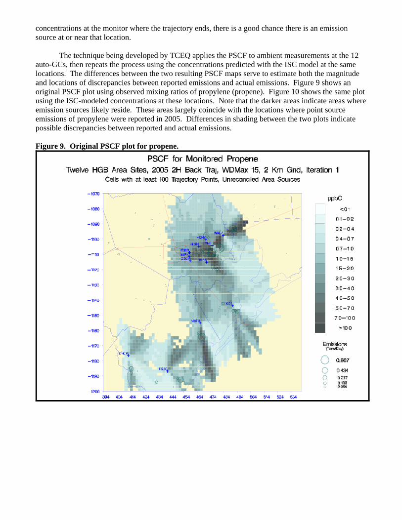
The technique being developed by TCEQ applies the PSCF to ambient measurements at the 12 auto-GCs, then repeats the process using the concentrations predicted with the ISC model at the same locations. The differences between the two resulting PSCF maps serve to estimate both the magnitude and locations of discrepancies between reported emissions and actual emissions. Figure 9 shows an original PSCF plot using observed mixing ratios of propylene (propene). Figure 10 shows the same plot using the ISC-modeled concentrations at these locations. Note that the darker areas indicate areas where emission sources likely reside. These areas largely coincide with the locations where point source emissions of propylene were reported in 2005. Differences in shading between the two plots indicate possible discrepancies between reported and actual emissions. Figure 9. Original PSCF plot for propene.

Figure 10. PSCF for ISC-modeled propene.

Generally, potential source areas are lighter than in the plot using measured concentrations, indicating that reported emissions do not fully explain measured concentrations. Taking the ratio of Figures 9 and 10 provides an estimate of how much additional emissions are needed and where, in order to reconcile the reported emissions with ambient concentrations. Figure 11 shows the ratio (monitored/ISC) for propene, in which the deeper the color, the higher the predicted multiplier needed for that grid cell. Note that the plot shows large areas of dark red which do not correspond to any point sources. The underlying discrepancies might be associated with area and/or mobile sources in these locations, or may simply be a result of proximity to large sources. In any case these areas have relatively low emissions compared with the larger point sources, so even a large ratio amounts to a fairly small discrepancy in total tons.

Figure 11. PSCF Ratio for propene, showing predicted multiplier required.

TCEQ has conducted some preliminary photochemical modeling using HRVOC emissions adjusted using the ISC/PSCF analysis and the results look promising. We are currently working on resolving the point sources from other emission sources in the analysis and expect to improve significantly on the results presented in this paper shortly. EI Improvement Projects

The Emissions Assessment Section of TCEQ has also attacked the under-reporting issue head-on from several angles. First is the ever-improving EI Guidance Document that instructs EI preparers on the main issues that QA staff will be looking for in reported annual EIs. Topics of recent special interest have been flares, equipment leak fugitives, and cooling towers. Additional guidance is provided not only in the EI Guidance Document, but at semi-annual workshops.

Flares are of major concern. There is much uncertainty, and TCEQ has discovered many

examples of flares that are labeled “emergency flares” that are operated more like routine thermal oxidizers. Topics for flares include flare minimization (i.e., what else can an operator do besides sending a stream to the flare) and DRE (destruction removal efficiency). Besides modifying our standard guidance on use of “default DRE”, TCEQ funds many studies, such as flare speciation modeling using current CFD (computational fluid dynamics) software and projects with manufacturers and industry to study design parameters and alternatives to flaring.

TCEQ is a leader in the use of remote sensing of emissions. We now have hands-on experience with Differential Absorption LIDAR (DIAL), HAWK infrared video camera flyovers, and GasFindIR cameras onsite. The GasFindIR camera has been such a hit with industry safety managers, that several have been purchased to not only find potential safety hazards (leaking flammable or toxic VOCs), but to identify more routine leaks.

TCEQ has found several previously unreported sources of enormous amounts of VOC. One of

these is Tank Landing Losses, originally found using a remote sensing technique. TCEQ discovered that many of the large tank farm operators (usually bulk tank-for-hire) allowed their floating roofs to land on the legs, allowing the volatile heel (leftovers in the bottom) to fill the head space and escape out the normal pathway of tank VOC loss. This amounted to more than 7000 tpy VOC increase in HGB alone. While these are rarely in HRVOC service, the total amount of VOC is significant. The retroactive emissions fees associated with these now-captured losses was significant. Similarly flash emissions from upstream oil and gas storage tanks amount to an estimate 80,000 tpy VOC increase in HGB and more than 750,000 tpy increase in statewide area source VOC emissions increase. Again, these were previously unreported, but the quantity of small oil and gas patches across Texas are enormous. Leaking barges in the intercoastal waterways or ship channels are another purported source of unreported or under-reported VOCs (again, not likely HRVOC, but may be in large quatity). The Coast Guard has agreed to maintain records of barge activity. CONCLUSIONS

TCEQ has adopted new rules into its SIPs that will better quantify and reduce HRVOC

emissions from four key industrial sources: fugitives, flares, process vents, and cooling towers. The adopted rules target HRVOC emissions. Analysis showed that limiting emissions of ethylene, propylene, 1,3-butadiene, and butenes in conjunction with an 80 percent reduction in NOX is equivalent or better in terms of air quality benefit to that resulting from a 90 percent point source NOX reduction requirement alone.

Ethylene, propylene, 1,3-butadiene, and butenes have been found to frequently cause high total reactivity conditions, and often dominate the total reactivity. Substantial emission reductions of these compounds are likely to make a large impact on high ozone, rapid ozone formation, and transient high ozone observed in the Houston area. Yet additional controls on many VOC sources will be necessary to reach attainment. TCEQ will continue to study VOC data available now and in upcoming years to determine whether additional compounds should be added.

Through the research conducted as a part of TexAQS and TexAQS II, HRVOC emissions have been acknowledged as a priority area needing both improved emission controls and better emission quantification. The enhanced monitoring requirements that have been established as part of the HRVOC rules will improve emission quantification. The HRVOC emissions in future models will be based on measured HRVOC emissions rather than on estimated emissions based on ambient ratios.

“What drives local ozone production?” This may be a changing answer that is already being addressed, as we transition away from the 1-hour ozone standard to the new 8-hour ozone standard for HGB. This is partially being addressed with the new ISC/PSCF emissions reconciliation technique in that the auto-GC data represent 8-hour averaging times. EI reconciliation is being addressed feverishly from an EI Improvement perspective, with many ongoing and proposed projects and contracts. The bottom line for modelers is that we can always use higher resolution data – better spatial precision, better temporal precision, and better chemical (speciation) precision.

REFERENCES 1. Estes, Wharton, Boyer, Fang, et al, TCEQ report, “Analysis of Automated Gas Chromatograph Data

from 1996-2001 to Determine VOCs with Largest Ozone Formation Potential“, Nov 2002 http://www.tceq.state.tx.us/assets/public/implementation/air/am/docs/hgb/tsd1/attachment6-agc_voc.pdf

2. Cantu, G; TCEQ Report, “Speciation of Texas Point Source VOC Emissions for Ambient Air Quality Modeling”; July 2003 ftp://ftp.tceq.state.tx.us/pub/OEPAA/TAD/Modeling/HGAQSE/Modeling/EI/PointEI_VOC_Speciation_Report-GabrielCantu.pdf

3. Carter, William, University of California at Riverside, latest database work, http://pah.cert.ucr.edu/~carter/emitdb/

4. Carter, William, University of California at Riverside, MIR reactivity scales, 2002 ftp://ftp.cert.ucr.edu/pub/carter/SAPRC99/r02tab.xls

5. Thomas, Ron, presentation, HEIRS referenced in http://www.tceq.state.tx.us/assets/public/implementation/air/am/committees/pmt_set/20070227/07.02.27-rthomas-ei_update.pdf

6. TexasAQS findings, Bibliography of Technical Support Information Reviewed and Considered for Dec 2002 SIP http://www.tceq.state.tx.us/assets/public/implementation/air/am/docs/hgb/tsd1/AppendixD-bibliography.pdf

7. TexAQS II findings, Bibliography on TCEQ webpage: http://www.tceq.state.tx.us/nav/eq/texaqsII.html

8. Smith, Jim and Jarvie, John, TCEQ, personal correspondence, 2008 KEY WORDS

TCEQ Texas Commission on Environmental Quality Highly Reactive VOC HRVOC TexAQS 2000 TexAQS II Houston-Galveston-Brazoria nonattainment area HGB Ozone modeling Photochemical modeling TCEQ SIP Emissions Reconciliation HRVOC Adjustment Olefin emissions Terminal olefins Auto-GC Speciation Reactivity Maximum Incremental Reactivity MIR Underestimated emissions William Carter December 2000 SIP December 2002 SIP

December 2004 SIP Remote Sensing

ACKNOWLEDGMENTS Many thanks to: My Coauthors – for assistance, peer review, support, previous presentations that I could borrow from TCEQ Emissions Assessment Section – for their great diligence at digging deeper for EI Improvement TCEQ Data Analysis/Field Study Team – for their management of TexAQS and their many analyses TCEQ Air Modeling Team – for acting as one of the best teams I know TCEQ Air Quality Division Managers – for giving me the time and support I needed to accomplish this TexAQS participating researchers – for coming to Texas in the heat of the summer, providing instrumentation, imparting expertise, presenting at workshops, and publishing results