embedding jit in mrp: the case of job shops

Journal of Manufacturing Systems Volume 13/No. 3

Embedding JIT in MRP: The Case of Job Shops Ziaul Huq, University of Nebraska-Omaha Faizul Huq, University of Texas-Arlington

Abstract The philosophy and principles needed to institute JIT

in any system, including a job shop, are described. A simulation model is developed using a benchmark job shop to study using a pull system in a job shop having variations in processing times, load levels, and machine breakdowns. It is inferred from simulation that JIT can be implemented if certain conditions are met. Processing time variations did not pose a serious impediment, but load levels and machine breakdowns were critical factors. With uneven loading, the resulting capacity bottlenecks make the pull system look like a push system. This can be avoided by processing a uniform mix of jobs to not violate workstation capacity limitations. If machine breakdowns are unavoidable, maintenance of buffer capacity is essential.

Keywords: MRP/JIT, Pull System, Simulation, Pro- cessing Time Variations, Level Load, Machine Break- down

Introduction The advantages of implementing just-in-time

(JIT) principles in a repetitive manufacturing system are well known. 1'2 Krajewski et al. 3 have shown that the success of a production system depends on the manufacturing environment, not the system. Reasons for the success of JIY can be ascribed more to the discipline required to implement the system than to the system itself. Broadly speaking, any manufacturing system can be described in terms of environmental requirements to implement the system, organizational requirements for planning and execution purposes, and control requirements for conducting day-to-day operations. The environmental condition in a job shop typically requires an MRP control system to manage its operations. Flapper, Miltenburg, and Wijngaard; a Miltenburg

and Wijngaard; s Discenza and McFadden; 6 and Belt 7 support integrating or phasing in JIT with MRP. While most strategic decision factors (such as waste reduction, total quality control, continual improvement, and transaction reduction) and many design and planning decision factors (such as reliable vendors, multifunctional workers, and foolproof methods) can be implemented in a job shop, many shop-level control decision factors of JIT are difficult to implement there. MRP and JIT are not incompatible systems. 4's Bullinger, Warnecke, and Lentes 9 see the progression from MRP to JIT as a precursor to computer-integrated manufacturing. The most obvious difference between MRP and JIT lies in management philosophy. JIY recognizes that a proprietary process is just as formidable a competitive weapon as a proprietary product. This research seeks to determine the necessary conditions for implementing the shop control features of JIT in a job shop, that is, to find what improvements are required in a job shop to reap the benefits of JIY (kanban) and, when implemented, to know the extent of improvement in job shop performance.

Most attempts to improve operations in a job shop focus on costly automation technologies or production control software such as closed-loop MRP or MRP II. Some job shop manufacturers have attempted to implement JIT by overhauling the existing manufacturing system overnight. Many of these manufacturers, after spending considerable resources on a JIT transition, have been disap- pointed with the results. 10 Such conversions must be gradual, and management must adopt policies and procedures that are consistent with the manufacturing environment of the job shop. This research will test the effect of variations in setup and job processing times, load levels, and machine breakdowns on JIT (kanban) performance. Because this

153


research deals only with the production control aspect of JIT, it will be referred to in the paper as a kanban system.

Huang, Rees, and Taylor l~ have shown that the JIT pull system looks like an American push system if JIT is implemented without creating the proper operating environment. Rice and Yoshikawa ~2 have emphasized that the success of a JIT system has its roots in employee motivation. Sarker and Harris 13 have found that without balance in the production system, JIT will fail. Philipoom et al. t4 have shown that without the proper manufacturing environment, JIT will be difficult to implement. Celley et al. is have identified top management and employee motivation, low setup times, high-quality incoming parts, reliable equipment, and a firm production schedule as the most important factors in JIT implementation. Practitioners recommend that for JIT implementation, group technology, uniform plant load, low setup times, preventive maintenance, and supplier participation are necessary. 16A7 A close examination of these requirements reveals that any improvement in manufacturing control factors will also benefit a job shop operation.

Flapper, Miltenburg, and Wijngaard 4 discuss how backflushing can be used in an embedded MRP/JIT system to control material by eliminating detailed MRP calculations. They suggest implementation of a pull system by using phantom items at the production process stage. In a JIT system, products move through the shop very quickly, and there is no need to track the items; however, in a job shop, scheduling requirements necessitate detailed job tracking. This research will attempt to delineate the conditions under which detailed job tracking will not be necessary in a job shop, thereby making the transition to a pull system easy.

In Support of MRP/JIT

Why JIT? The principles, system, and structure of JIT are

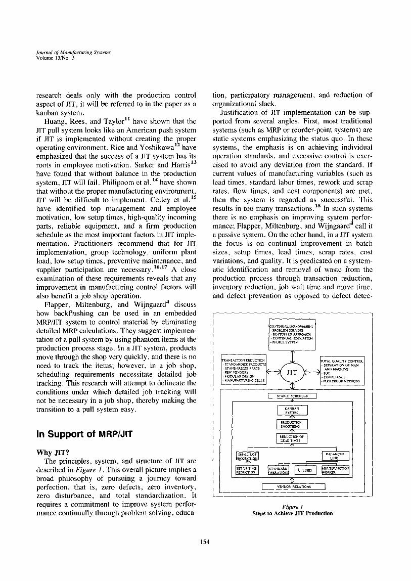
described in Figure i. This overall picture implies a broad philosophy of pursuing a journey toward perfection, that is, zero defects, zero inventory, zero disturbance, and total standardization. It requires a commitment to improve system performance continually through problem solving, educa-

tion, participatory management, and reduction of organizational slack.

Justification of JIT implementation can be sup- ported from several angles. First, most traditional systems (such as MRP or reorder-point systems) are static systems emphasizing the status quo. In these systems, the emphasis is on achieving individual operation standards, and excessive control is exer- cised to avoid any deviation from the standard. If current values of manufacturing variables (such as lead times, standard labor times, rework and scrap rates, flow times, and cost components) are met, then the system is regarded as successful. This results in too many transactions.18 In such systems there is no emphasis on improving system performance; Flapper, Miltenburg, and Wijngaard 4 call it a passive system. On the other hand, in a JIT system the focus is on continual improvement in batch sizes, setup times, lead times, scrap rates, cost variations, and quality. It is predicated on a system- atic identification and removal of waste from the production process through transaction reduction, inventory reduction, job wait time and move time, and defect prevention as opposed to defect detec-

CONTINUAL IMPROVEMENT I - PROBLEM SOLVING - BOTTOM UP APPROACH - CONTINUAL EDUCATION - PEOPLE SYSTEM

I ~TAELE ~C~E I

KANBAN I SYSTEM

,'r, ]PRODUCTION] S MOOTH~G

I, J REDUCTION OF LEAD TIMES I

q, I

I'L E° I

VENDOR RELATIONS [

Figure 1 Steps to Achieve J IT Product ion

154


tion. It is an active 4 or dynamic system. There is no performance standard for the system; it is a journey rather than a destination.

Second, the pull signal in the JIT system has the effect of regarding the next process as a customer of the previous process. This concept is extremely useful in implementing total quality control. It min- imizes both internal and external cost of bad quality and relinquishes the necessity to track jobs through the facility. In the traditional facility, items are pushed through the shop floor without any regard for the next process, and there is no customer focus within the manufacturing process. In such systems, total quality control programs are difficult to implement and frequently fail to achieve desired results.

Finally, JIT uses an enforced problem-solving approach. Because inventory is reduced to a mini- mum, the system cannot tolerate any interruption; therefore, extreme care is taken to root out any production problems. In traditional MRP and reorder-point systems, no such incentive to solve production problems is available. Inventory not only hides problems, but it dramatically increases operating expenses.

Problems with Job Shops Beyond rough-cut capacity planning, MRP can-

not cope with the dynamics of floor activities in a job shop. To cope with uncertainties, MRP uses very long lead times to develop the production schedule by considering worst-case scenarios. The lead times tend to get longer over time as shop control personnel face short-run uncertainties and bottlenecks. Because MRP is a passive system, 4 no attempt is made to improve the long lead times and the high inventories that result from it. Based on their experience at the Schlumberger job shop, Ashton and Cook ~9 and Ashton, Johnson, and Cook z° report that closed-loop MRP systems do not work in a job shop. They argue that the time response of the MRP replanning procedure is slower than the rate of change of the error function. The lot sizing decision in MRP is based on established lead times, especially setup times, that are biased to be safe, thus resulting in big lot sizes. In addition, by having the attitude of being safe in meeting the schedule, especially for component parts, needed parts arrive at the final assembly sometimes months in advance, resulting in high component invento-

ties. On the other hand, because of the fixed nature of MRP parameters, operations on some component parts are delayed or not started soon enough. This often results in some jobs being expedited while other jobs are delayed. JIT does not treat any system parameter as fixed; the continual improvement philosophy of JIT does not follow any standard.

MRP production scheduling systems sequence jobs without considering available finite capacity. Sched- ules are adjusted by adding a routine clean-up procedure (called bottom-up replanning) in which capacity requirements are evaluated and pegging data are used to resolve material shortage problems. There- fore, MRP uses a two-step procedure to implement a production plan. JIT combines these two steps into one by simply considering a limited capacity. In JIT, the kanban or pull signal is used to control capacity. Job shops are basically labor-constrained; in many job shops, labor levels are not planned realistically. If schedules are not met, labor productivity alone does not improve shop performance.

Many job shops fail to achieve desired efficiency for several reasons. First and foremost is the ten- dency to run special orders, a practice that offsets the balance in the shop and creates MRP nervous- ness. This unique nature of a job shop precludes implementation of a pull system. A large number of job shop manufacturers do not produce items in volume. Many companies have production operations that are not under the same roof. Sometimes the final assembly schedule is not level enough to provide reasonable pull signals to the workstations supplying it. Consumption of a small part by the final assembly may be so low that it may not be reasonable to maintain a pipeline stock of the part to feed the final assembly. It may be necessary to start a fabrication process in advance of any pull signal because it is impossible to reduce setup time for the process. Some machines in the production facility may be general-purpose. Setting up these machines may require hours or even days. Therefore, it would make sense to run large lots in such an environment.

An option that may alleviate some of these problems is mixed-model processing, if the plant can create a stream of nonrandom orders out of the chaos in the marketplace. This would be an advantage in a low-capacity process with inexpensive equipment and low setup times. 21 To implement mixed-model processing, product designs must

155


exist at order-entry time, any engineering changes must be grouped to avoid random ripples cascading through the process, and supplying processes must deliver quality materials on time. zz If these conditions are not met, then no amount of scheduling magic can create conditions for JIT in a job shop.

Research Methodology Simulation of a hypothetical job shop is used as

the research methodology because it makes the results of the study more generalizable than the use of a model of any particular shop; however, the hypothetical model is developed by using a benchmark job shop that produces 42 different varieties of parts for field turf vehicles. The hypothetical model does not incorporate many of the exogenous variables that influence performance of the benchmark job shop. This is consistent with the aim of the study: to test the effect of setup and processing time variations, load levels, and machine breakdowns on a JIT pull system in a job shop, rather than to confound the effects of exogenous variables with the effects of control variables. It should be men- tioned here that the most obvious differences between a hypothetical and actual shop (for exam- ple, number of workcenters, number of machines, pattern of workflow, and so on) have been found to be of little consequence in determining the relative importance of different operating policies. Studies conducted by Baker and Dzielinski, z3 Conway and Maxwell, z4 Moore and Wilson, 25 and Ragatz and Mabert z6 support this conclusion. In addition, use of a hypothetical model has the advantage of being more readily linked to previous research.

This study seeks to determine at what levels of variations in setup and processing times, load imbalance, and machine breakdowns a transition to a pull system is appropriate in a job shop to make MRP/JIT a valid choice. Five levels of setup and processing time variations, two levels of load factors, and three levels of machine breakdowns are selected for testing. The five levels of setup and processing time variations are represented by no variation, exponential processing times, 25% coefficient of variation (CV), 50% CV, and 75% CV. The reason for selecting such tight variation levels is because JIT (kanban) is a very rigid system and can

tolerate very little variation from its set parameters. The two selected shop load levels are based on actual processing of master production schedule (MPS) quantities for the benchmark job shop without any rough-cut capacity planning, and on processing the same jobs with rough-cut capacity planning so that there is uniform load on the workstations. Only three levels of machine breakdowns are tested (no breakdown and 10% and 25% probability of breakdown) because JIT (kanban) can tolerate very little interruption.

Measures of performance used are the time- averaged inventory values for the studied systems. In addition, relevant service-level performance indi- cators-average tardiness and proportion of tardy jobs--are also collected. The reason for collecting time-averaged inventory values is because the products are not equally valued, and the value added after each operation is different for each product. A simple sum of the number of units in inventory assumes equal product value, and it fails to take into account product structures and multiplicities. Detailed product cost data was collected from the benchmark job shop for use as input to the simulation program. This approach is consistent with the dollar-weighted measure of Wilson and Mardis 27 and the stock-level performance indicator of Grun- wald, Striekwold, and Weeda. 2s Data are collected on system inventory values that comprise the sum of initial inventory before any processing, work- in-process (WIP) inventory, and completed inventory that is still in the system because due dates have not been reached. In addition, data on WlP inventory are collected separately to determine which parameter combination supports reduction of WIP. Also, data on average backlog and average utilization of workstations are collected to compare shop load levels. The following sections describe the benchmark shop used in the simulation model, the simulation program, and data collection and analysis procedures.

Shop Description The job shop used in the study has six worksta-

tions, each with multiple machines. There are 23 machines and 23 workers in the shop. (See Table 5 for a description of the shop along with the shop utilization.) The shop is used for processing 42 different parts for use in the field vehicles produced

156


by a Midwest manufacturer. It is a job shop environment with each job having an independent processing route. Some jobs visit the same workstation several times. The shop structure described above is consistent with that used by Baker and Dzielinski 23 and Baker and Bertrand. 29

The routing and number of operations for each type of job are fixed. The number of operations per job varies from two to eight. Actual data were collected from the study shop on job routings, setup times, job processing times at various workstations, and the value added to jobs at various stages of processing. These were used as inputs to the simulation model. Analysis of job interarrival times (MPS job orders) reveals an approximately exponential distribution with a mean of 60 minutes. Jobs arrive in batches of 20-100 jobs of a particular type, with the average batch size varying around 50. Details of the shop and inputs to the simulation model can be found in Huq. 3°

Simulation Model The study was carried out using a discrete event

simulation model of the job shop. The simulation program was written using the S1MSCRIPT 11.5 simulation language. Figure 2 is a flowchart of overall simulation logic and describes the lifecycle of a container of jobs as it moves through the facility. A one-card kanban (or kanban square) system is implemented in the model. The container size is determined based on MPS quantities for the parts over a six-month period; it is consistent with the average batch size processed by the study shop. The model uses the first-come first-serve rule to dispatch jobs and the total work content rule to set job due dates, rules consistent with JIT shop control procedures. Details of the simulation program are omitted for the sake of brevity; interested readers are referred to Huq. 30

The most important problem facing a real-world simulator is determining whether a simulation model is an accurate representation of the actual system being studied. Because the developed model is hypothetical, the problem is one of verification rather than validation. The model was developed in stages. At every stage, SIMSCRIPT library commands were used to obtain a dynamic map of the function and subroutine calls that are being executed. After the program was debugged, it was verified whether the

"Define data stPF~'A/'V~rrrtJctures "Define entities,llttributes,

sets and re at onsh p6 J

~ INITIALI~TII~I Clean up system

"Job generat~n in block s "Assignment of job attributes [ *Set job allowances by TWK J k ~ READ J "File jobs in PRESHOPFILE ~ DATA J "Rank jobs in PRESHOP FILE I I

"Generate Pull Signals : Transfer jobs form PRESHOP

FILE to BACKLOG FILE ; Select Container Size : Use FCFS dispatching rule : Release jobs based on pall signaJ

*Set transient period

Select Job Route [

work ~ sta

I File Job in ~mplet~ inven ory

t I Call inventory shipment

rules: destroy jobs if due dates are reached

J Discard lransient data

, t aJ DATA v J COLLECTION

Figure 2 JIT (Kanban) Simulation Flowchart

simulation model was operating as intended. The model was run for a few hours so that its output could be verified manually. In addition, with the help of SIMSCRIPT library routines, it was possible to verify the event and process notices. Detailed tracking of job batches through the shop verified that the program was performing as expected.

Data Collection and Analysis Because it is a nonterminating system, steady-

state results were collected for analysis. There are no statistical procedures for doing this. Authors

3~ such as Conway, Emshoff and Sission, 32 Law and Kelton, 33 and Hoover and Perry 34 have used rules of thumb; they suggested that initial observations should be thrown away as long as they seem to

157


increase or decrease steadily. Theoretically, before the steady state is reached, the mean of the difference (first difference, Ax i) between the successive daily average inventory should be nonzero (some positive value), and it should converge to zero after the steady state. This is statistically verified by performing the " t " test with the standard deviation(s) estimated from the sample data. 35'36 Analy- sis of the simulation output shows that the steady- state condition is reached when the program is run for about 30 simulated days.

Common random number streams are used across comparisons to estimate performance of shop parameter combinations. This assures that any observed differences in shop performance are due to the effect of tested shop parameter combinations rather than to fluctuations of experimental conditions. Use of common random numbers also serves as a variance reduction technique, which helps reduce the sample size, that is, the number of replications. The number of replications of each simulation is determined based on the relative-half confidence interval approach. 33 Based on this approach, it is determined that 30 replications are needed to achieve the desired confidence and accu- racy in the simulation output. Consequently, steady-state data on time-averaged daily inventory values for each inventory category are collected for 30 days, with each simulation day representing 16 hours of operation (two shifts at the benchmark shop). Simulation outputs are examined with analysis of variance and multiple comparison tests.

Analysis of Simulation Results In the following sections, results of the simula-

tion experiments are analyzed. Shop parameters tested are variations in setup and processing times, load leveling through uniform mix of jobs, and machine breakdowns. First, results of experiments with variations in setup and job processing times are analyzed. Next, experiments combine load leveling with processing time variations, and finally, these are combined with machine breakdowns.

JIT Performance with Variations in Processing Times

In these simulation runs, no load leveling was applied and no machine breakdown was assumed.

The model processed MPS quantities for the benchmark shop as demand occurred. Figure 3 presents system and WIP inventory levels for various processing time variations. System and WIP inventories exhibit similar trends. Within a certain range of coefficient of variation (CV) values, that is, 0-50%, both system and WIP inventory values do not vary much; however, higher variations in processing times (CV > 50%) tend to have a negative effect on WlP inventory. This is confirmed by analysis of variance (ANOVA) and Duncan's multiple range tests shown in Tables 1 and 2.

Table 1 reveals no significant difference in system inventory value between tested processing time variations; however, the Duncan's multiple range test puts system inventory results for no processing time variations and for processing times of CV 75% in separate categories, indicating that they are significantly different. In Table 2, ANOVA and multiple range tests for WIP inventory are presented. Although the F value demonstrates a significant difference in WIP inventory for variations in setup and processing times, the Duncan's multiple range test places CV 50%, CV 25%, and no variation

30000

25000-

20000

15000

10000

5000

30000-

25000"

20000'

15000"

~0000"

5000"

0 0

Expor~ntml ~xocgssing time

cv-25% CV-50%

CV-75%

• , . , . = , 10 20 30 40

Day (Repbcaton) Number

t . . . . . . . No variation in processing time

~ Exponential p~oce=sing time CV-25% CV-50%

CV-75%

1 0 2'0 30 4O

Day (Replicatior~) Number

Figure 3 System Inventory Value and WIP Inventory Value for

Variations in Job Processing Times

158


Table 1 Comparison of System Inventory Values for Variations in

Processing Times With No Load Leveling

Analysis of variance procedure

Dependent Variable: System inventory value (NSYS)

Source DF Sum of SQ Mean SQ F Value Pr • F

Model 4 304077 760.19 191 0.11 Error 145 57784.70 398.51

Duncan's multiple range test for variable: NWIP note: This test controls the type I comparisonwise error rate,

nol the experimentwise error rate

Alpha = 0.05 DF = 145 MSE = 398.51

Number of Means 2 3 4 5 Critical Range 10.24 10.77 11.11 11.36

Means with the same letter are not significantly different.

Duncan xroupin z ~ N Method

A 124.07 30 CV = 75 % A

B A 121.13 30 Exponential processing time B A B A 116.76 30 CV = 50 % B A B A 113.20 30 CV = 25 % B B 112.40 30 No processing time variation

Table 2 Comparison of WIP Inventory Values for Variations in

Processing Times With No Load Leveling


Dependent Variable: Work in process inventory value (NWIP)

Source DF Sum of SQ. Me~m SQ. F Value Pr > F

Model 4 6542.77 1635.69 3.15 0.01 Error 145 75253.90 518.99

Duncan's multiple range test for variable: NWIP note: This test controls the type I comparisonwis¢ error rate,

not the experimentwise error rate

Alpha = 0.05 DF = 145 MSE = 518.99

Number of Means 2 3 4 5 Critical Range I 1.69 12.29 12.68 12.97


Duncan m'ouDine Mean N Method

A 117.96 30 CV = 75 % A A 114.50 30 Exponential processing time A

B A 107.63 30 CV = 50 % B B 102.16 30 CV=25 % B B 101.30 30 No processing time variation

in the same category. Results for system inventory (Table 1) are similar. Analysis reveals that the JIT (kanban) system is not as sensitive as thought to be in terms of variations in setup and processing times. In a shop environment where time variations remain within a reasonable limit, JIT (kanban) can be suc- cessfully implemented without incurring much pen- alty in terms of higher inventory levels.

Because no load leveling was applied in these simulations, both inventory and due date performance (see Table 6) for these experiments are poor compared to performance with load leveling. With exponential processing time and a higher CV (75%), the proportion of jobs tardy and the average tardiness is much higher. The same due date measures for a CV in the 50% range are in close proximity to each other. Again it can be inferred that with lower variations in setup and processing times, reasonable JIT (kanban) performance can be achieved in a job shop.

JIT Performance with Load Leveling In a typical job shop, orders are processed as their

demands occur. Little care is taken to level workstation loads through rough-cut capacity planning. In the following simulation experiments, actual MPS quantities are not immediately released to the shop. The daily mix of job arrivals had a skewed distribution that put excessive loads on certain

workstations. A rough-cut capacity plan confirmed that for a balanced load a uniform mix of jobs must be processed by the shop, or the mix of jobs should be such that bottlenecks are not created. For the study shop, a mixed-model processing approach assured a level load. The new MPS created through rough-cut capacity planning released a uniform mix of jobs every day to the shop for processing. See Table 5 for shop utilization levels for the simulated shop with and without load leveling. Without load leveling there is excessive load on workstations 2 and 5; in particular, workstation 2 has become a bottleneck. With load leveling, the bottleneck is removed and backlogs have been reduced to toler- able sizes.

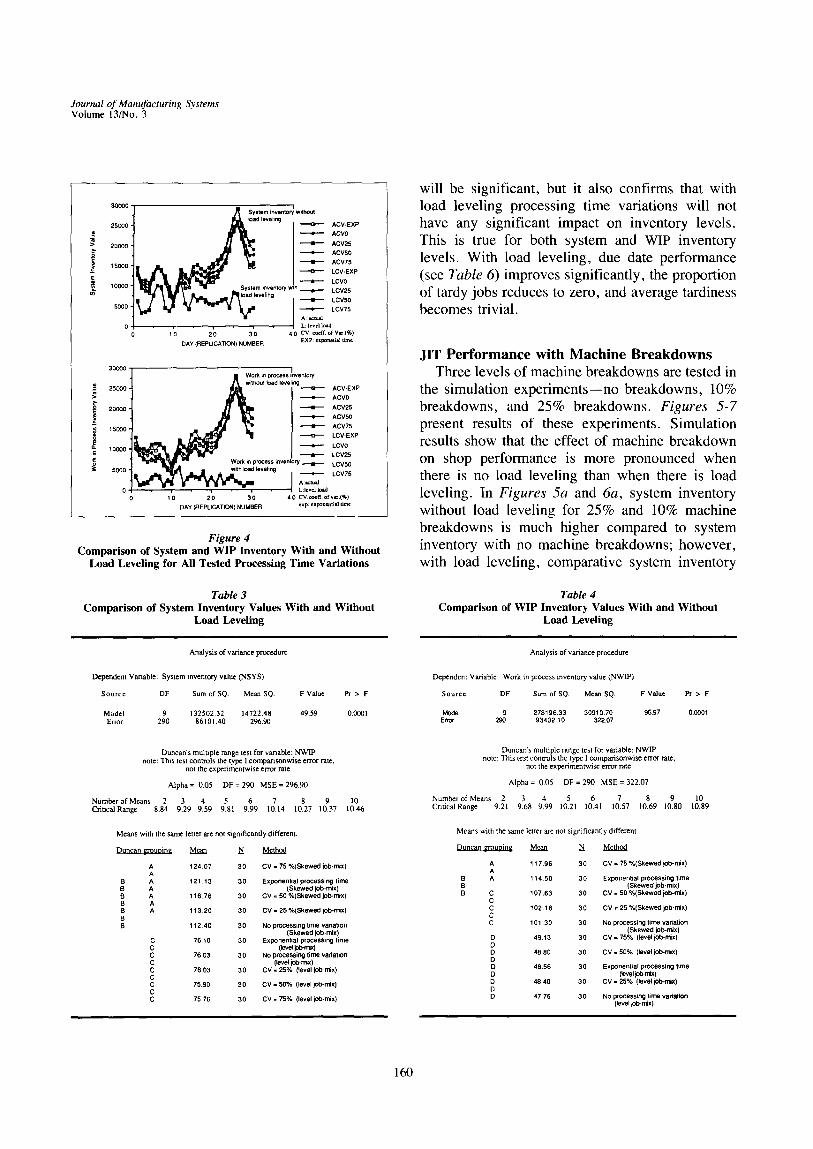
In Figure 4, system and WIP inventory levels with load leveling are compared with inventory levels without load leveling. Both system and WIP inventory levels improve significantly with load leveling. In Tables 3 and 4, ANOVA and Duncan's multiple range tests for these runs are carried out. There is a significant difference between inventory levels with and without load leveling, as confirmed by the significant values of F in the ANOVA test; however, the Duncan's multiple range test points to some more interesting results. All combinations of processing time variations and load leveling are placed in the same group. This not only confirms that with load leveling the reductions in inventory

159


System inventory without

25000 load leveling ~ ACV-EXP

a ACVO

el ACV25 20000 • ACVBO

• ACV75 15COO " - - -O-- - LCV-EXP

A ,, , LCV0 10000 System inventory ~ & . LCV25

load leveling • LCVS0

5000 A: ~m=l LCV75

0 l • , • i ' , • L: level lord 0 1 O 20 30 40 CV: coeff, of VK.(%)

BAY {REPLICATION) NUMBER EXP: exponetiad time

Work in prooDss inventory without load leveling

25000 ---t~, ACV-EXP ACVO

20000 : ACV25 ACV50

15CO0 • ACV75 ~ LCV-EXP

=" 10CO0 LCVO -¢ LCV25 ~o Work in process inventory • LCVS0

$000 with load leveling

0 , ~ : , 7 . % . , 0 10 20 30 40 CV:~ f f . of v=.(~)

DAY (REPLICATION) NUMBER exp: ¢xpon~ntitl time

Figure 4 Comparison of System and WIP Inventory With and Without

Load Leveling for All Tested Processing Time Variations

Table 3 Comparison of System Inventory Values With and Without

Load Leveling


Dependent Variable: System inventory value (NSYS)

Source DF Sum of SQ. Mean SQ. F Value Pr • F

Model 9 132502.32 14722.48 49.59 0.0001 Error 290 86101.40 296.90

Duncan's multiple range test for variable: NWIP note: This test conrz'ols the type I comparisonwise error rate,

not the experimentwise error rate

Alpha = 0.05 DF = 290 MSE = 296.90

Number of Means 2 3 4 5 6 7 8 9 10 CriticalRange 8.84 9.29 9.59 9.81 9.99 10.14 10.27 10.37 10.46

Means with the same letter are not significandy different.

Duncan ~ouoine Mean N Method

A 124 07 30 CV = 75 */.(Skewed job-mix) A

13 A 121,13 30 Exponential processing time B A (Skewed job-mix) B A 11676 30 CV = 50 %(skewed job-mix) B A B A 113.20 30 CV = 25 %(Skewed job-mix) B B 112,40 30 No processing time variation

(Skewed job-mix) C 76,10 30 Exponential processing time c (leve~ ~o~x) C 7603 30 NO processing time variation C (level job-mix) C 76,03 30 CV = 25% 0evel job-mix) C C 75.90 30 CV = 50% (level job-mix) C C 7576 30 CV = 75% (level job.mix}

will be significant, but it also confirms that with load leveling processing time variations will not have any significant impact on inventory levels. This is true for both system and WIP inventory levels. With load leveling, due date performance (see Table 6) improves significantly, the proportion of tardy jobs reduces to zero, and average tardiness becomes trivial.

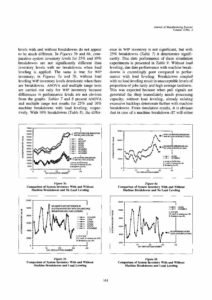
JIT Performance with Machine Breakdowns Three levels of machine breakdowns are tested in

the simulation experiments--no breakdowns, 10% breakdowns, and 25% breakdowns. Figures 5-7 present results of these experiments. Simulation results show that the effect of machine breakdown on shop performance is more pronounced when there is no load leveling than when there is load leveling. In Figures 5a and 6a, system inventory without load leveling for 25% and 10% machine breakdowns is much higher compared to system inventory with no machine breakdowns; however, with load leveling, comparative system inventory

Table 4 Comparison of WIP Inventory Values With and Without

Load Leveling

Analysis of variance pr(w.edure

Dependent Variable: Work in process inventory value (NWIP)

Source DF Sum of SQ. Mean SQ. F Value Pt > F

Model 9 278196.33 30910.70 9~.97 00001 Erro¢ 290 93402 t 0 32207

Duncan's multiple range test for variable: NWIP note: This test controls the type I comparisonwis¢ error rate.

not the experiment.vise error rate

Alpha = 0.05 DF = 290 MSE = 322.07

Number of Means 2 3 4 5 6 7 8 9 10 Critical Range 9.21 9.68 9.99 10.21 10.41 10.57 10.69 10.80 10.89


Duncan Eouoin~ Mean N Method

A 117.96 30 CV = 75 %(Skewed job-mix) A

B A 11450 30 Exponential processing t ime 13 (Skewed job-mix| B C 107.63 30 CV = 50 %(Skewed job-mix)

C C 10216 30 CV = 25 %(Skewed job-mix) C C 101 3 0 30 NO processing time variation

(Skewed job-mix) D 4913 30 CV = 75% (level jo~mix) O D 48.80 30 CV = 50% (level job-mix) D D 48,56 30 Exponential processing time D (~vei pt>mix) D 4840 30 CV = 25% (level job-mix) D D 47.76 30 NO processing time vadatlon

(level iCb-mix)

160


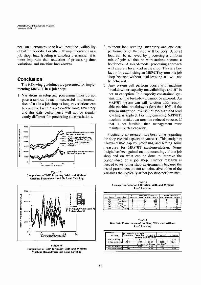
levels with and without breakdowns do not appear to be much different. In Figures 5b and 6b, comparative system inventory levels for 25% and 10% breakdowns are not significantly different than inventory levels with no breakdowns when load leveling is applied. The same is true for WIP inventory; in Figures 7a and 7b, without load leveling WIP inventory levels deteriorate when there are breakdowns. ANOVA and multiple range tests are carried out only for WIP inventory because differences in performance levels are not obvious from the graphs. Tables 7 and 8 present ANOVA and multiple range test results for 25% and 10% machine breakdowns with load leveling, respec- tively. With 10% breakdowns (Table 8), the differ-

ence in WIP inventory is not significant, but with 25% breakdowns (Table 7) it deteriorates significantly. Due date performance of these simulation experiments is presented in Table 9. Without load leveling, due date performance with machine breakdowns is exceedingly poor compared to performance with load leveling. Breakdowns coupled with no load leveling result in unacceptable levels of proportion of jobs tardy and high average tardiness. This was expected because when pull signals are generated the shop immediately needs processing capacity; without load leveling, already existing excessive backlogs deteriorate further with machine breakdowns. From simulation results, it is obvious that in case of a machine breakdown JIT will either

70000 , l% 65000 "l 60000 "] S ' ~ " = I ~ WI3H 2 5 1 MACHINE BREAKDOWN AND NO LOAD LEVELING 55000 -I I 50000 -I ~ ACV0

t ACV-EXP 45OO0 ACV25

ACV50 40000 • ACV75 35000 ~ ACV25B25 30000 " ,I. ACV75B25 25000 1 ~ ACV50B25 20000 NO MAvHINE BREAKDOWN

w'v "ii 15000 AND NOz LOAD LEVELING 10000 A:~t~zd. no load lovelm B

CV:cQeff. of vlfild¢~ (M • %) 5000 e~dow'n (Ps t %)

L 0 10 20 30 40

DAY (REPLICATION) NUMBER

40000

20000

10000

j~II~I~ NO MAI~I~ ~ AND

I ~ / ~ I~ ~ - • A CVSOB10 = t l = t A: acm=L no load kvdmg

CV: ¢oeff. of v m i l d o n ( i t • %) B: Breakdown (~ • %)

I 10 20 30 40


Figure 5a Comparison of System Inventory With and Without

Machine Breakdowns and No Load Leveling

Figure 6a Comparison of System Inventory With and Without


12000 i

1 ~ NO SIGNIFICANT DIFFERENCE IN I 10000 I ~ ~ SYSTEM INVENTORY WITH 25% MACHINE

2 0 0 0 • %)

B: B r e a k d o w n (as • %)

o , I o ,.0 2'o 3'0 . o

o.~ (.E.OO.T,ON> N U ~ .

12000

10(300

8000

6000

4000

2000 • = • = i

1 0 20 30 DAY (REPLICATION) NUMBER

I LCV50

- LCV50810 L: level ] o l d

C V : ¢oeff . o f v ='iW.ion ( • a 'It) B: Bre~edov,~ (== • %)

NO DIFERENCE AFTER LOAD LEVELING (CV-B0%)

I 4 0

Figure 5b Comparison of System Inventory With and Without

Machine Breakdowns and Load Leveling

Figure 6b Comparison of System Inventory With and Without


161


need an alternate route or it will need the availability of buffer capacity. For MRP/JIT implementation in a job shop, load leveling is absolutely essential; it is more important than reduction of processing time variations and machine breakdowns.

Conclusion The following guidelines are presented for imple-

menting MRP/JIT in a job shop:

1. Variations in setup and processing times do not pose a serious threat to successful implementation of JIT in a job shop as long as variations can be contained within a reasonable limit. Inventory and due date performance will not be significantly different for processing time variations.

700O0

,00o0 ~ w,;7o~g.~ ~.o~.,.~..~ow.. 50000 ~ ACV0 A: ~'tu~. ~ b~ld I~eLLn

ACV-EXP CV: coeff, of Vlc~ifim (%) . ov%, B:a,o.~,..~, 40000 AC 5 • i ,ov,5 :E . . . . .

30o0o ~ . ---o--- Acws~s

' ~ A N D NO LOAD LEVELING

0 I - 0 10 20 30 40


Figure 7a Comparison of WIP Inventory With and Without


8000

~ 6000

4000

z 200o

t'o 2'0 ~'0 DAY (REPLICATION)NUMBER

=

• - - - - 'B--- - LCV25 Bt LCV50

LCV75 = LCV25B25 • LCV50B25

LCV75B25 L : Level load CV: Coefficient of Variation (as a %) B : Breakdown (as a %)

4 0

Figure 7b Comparison of WIP Inventory With and Without


2. Without load leveling, inventory and due date performance of the shop will be poor. A level load can be achieved by processing a uniform mix of jobs so that no workstations become a bottleneck. A mixed-model processing approach will ensure a level load in the shop. This is a key factor for establishing an MRP/JIT system in a job shop because without load leveling JIT will not be achieved.

3. Any system will perform poorly with machine breakdown or capacity unavailability, and JIT is not an exception. In a capacity-constrained system, machine breakdown cannot be allowed. An MRP/JIT system can still function with reasonable machine breakdowns (less than 10%) if the system utilization level is not too high and load leveling is applied. For implementing MRP/JIT, machine breakdown must be reduced to zero. If that is not feasible, then management must maintain buffer capacity.

Practically no research has been done regarding the shop control aspects of MRP/JIT. This study has narrowed that gap by proposing and testing some measures for MRP/JIT implementation. Some insight has been gained on implementing JIT in a job shop and on what can be done to improve the performance of a job shop. Further research is needed to test other shop environments because the tested parameters are not an exhaustive of set of the variables that typically affect job shop performance.

Table 5 Average Workstation Utilization With and Without

Load Leveling

Worn Station WS1 WS2 w ~ W ~ W ~ WS6

Machine Type Laser Pre~ Pre~ Brake Weldinq Punch Press Sheann,q Bendinq Rolhnc

# of Averaoe Backloa fBalches) Machines Wilh load leveling Without

4 22 41 5 ~ 18~ 4 41 111 5 12 17 2 158 235 3 21

Averaae ~ilz ationf%} With load leveling, Wlthoul

73 IGO 64 79 44 44 80 85 53 63

Table 6 Due Date Performance of the Shop With and Without

Load Leveling

No Processing Exponenlial P Or I meV'°=nlP ...... "qOV=25°'olcv=80°'olov=' °'o

Percent of jobs tardy

W, hload, g I 0 . . . . . . I 0 i 03 i o i o3z Without load leveling 28.15 42.80 2 4 33.83 4611

Average t a r d i n e s s (in days )

hOad,ev. I o.2, I o22 I o.22 I o.2o I 0.2, Without load leveling 0.89 1 24 0.92 1.05 1.40

162


References 1. Y. Monden, Toyota Production System: Practical Approach to

Production Management (Norcross, GA: Industrial Engineering and Management Press, 1983).

2. Richard J. Schonberger, World Class Manufacturing (New York: The Free Press, 1986).

3. Lee J. Krajewski et al., "Kanban, MRP and Shaping the Manufacturing Environment," Management Science (v33, nl , 1987), pp39-57.

4. S.D.P. Flapper, G.J. Miltenburg, and J. Wijngaard, "Embedding JIT into MRP," International Journal of Production Research (v29, n2, 1991), pp329-341.

5. J. Miltenburg and J. Wijngaard, "Designing and Phasing in Just-in-Time Production Systems," International Journal of Produc- tion Research (v29, nl , 1991), pp115-131.

6. R. Discenza and F.R. McFadden, "The Integration of MRP II and JIT through Software Unification," Production and Inventory Management (n29, 1988), pp49-53.

7. B. Belt, "MRP and Kanban--A Possible Synergy?" Production and Inventory Management (n28, 1987), pp71-80.

8. J.C. Wortmann and W. Mohemius, "Kanban--Its Use as a Final Assembly Scheduling Tool Within MRP," Operational Research '84, J.P. Brans, ed. (Amsterdam: Elsevier, 1984).

9. H.J. Bullinger, H.J. Warnecke, and H.P. Lentes, "Toward the Factory of the Future," International Journal of Production Research (n24, 1986), pp697-741. 10. G.J. Bose and A. Rao, "Implementing JIT with MRP II Creates Hybrid Manufacturing Environment," Industrial Engineering (n20, 1988), pp49-53. 11. Philip Y. Huang, Loren P. Rees, and Bernard W. Taylor, "A Simulation Analysis of Japanese Just-in-Time Technique (with KAN- BANS) for a Multiline, Multistage Production System," Decision Sciences (v4, n3, 1983), pp326-344. 12. James W. Rice and Takeo Yoshikawa, "A Comparison of Kanban and MRP Concepts for the Control of Repetitive Manufactur- ing Systems," Production and Inventory Management (nl, 1982), ppl-13.

Table 7 Comparison of WIP Inventory Values With Processing Time

Variations and 25% Machine Breakdowns With Load Leveling


Dependent Variable: work in process inventory value

Source DF Sum of SQ. Mean SQ. F Value Pr > F

Model 5 4817.66 963.53 6.86 0.0001 Error 174 24432.71 140.41

Duncan's multiple range test for variable: NWIP note: This test controls the type ] comparisonwise error rate,

not the experiment,vise error rate

Alpha = 0.05 DF = 174 MSE = 140.41

Number of Means 2 3 4 5 6 Critical Range 6.08 6.39 6.59 6.74 6.87


Duncan Lrrouvin~ M ¢ ~ N

A 60.927 30 A A 58.900 30 A A 55.283 30

B 49.144 30 B B 48.818 30 B B 47.825 30

Method

C V - 7 5 % . B r e a k d o w n - 2 5 %

CV-25%,Breakdown-25%

C V - 5 0 % , B r e a k d o w n - 2 5 %

CV-75%, No breakdown



13. Bhaba R. Sarker and Roy D. Harris, "The Effect of Imbalance in a Just-in-Time Production System: A Simulation Study," Interna- tional Journal of Production Research (v26, n 1, 1988), pp 1-18. 14. Patrick R. Philipoom et ai., "An Investigation of the Factors Influencing the Number of Kanbans Required in the Implementation of the JIT Technique with Kanbans," International Journal of Production Research (v25, n3, 1987), pp457-472. 15. A.F. Celley et al., "Implementation of JIT in the United States," Journal of Purchasing and Materials Management (n22, 1986), pp9-15. 16. J. Williams, "Just-in-Time Ideally Suited to Smaller Manufac- turing Operations," CPA Journal (v55, 1985), pp81-83. 17. V.K. Kapoor, "Converting to JIT," Production Engineering (Feb. 1987), pp42-47. 18. Thomas E. Vollmann, William L. Barry, and Clay D. Whybark, Manufacturing Planning and Control Systems (Homewood, IL: Irwin, 1988). 19. James E. Ashton and Frank X. Cook, "Time to Reform Job Shop Manufacturing," Harvard Business Review (n2, 1989), ppl06-111. 20. J.E. Ashton, M.D. Johnson, and F.X. Cook, "Shop Floor Control in a System Job Shop: Definitely Not MRP," Production and Inventory Management Journal (n2, 1990), pp27-31.

Table 8 Comparison of WIP Inventory Values With Processing Time

Variations and 10% Machine Breakdowns With Load Leveling


Dependent Variable: work in process inventory value

Source DF Sum of SQ. Mean SQ. F Value Pr > F

Model 5 512.62 102.52 0.75 0.585 Error 174 23689.92 136.15

Duncan's multiple range test for variable: NWIP note: This test controls the type I comparisonwise error ram,

not the experiment'wise error rate

Alpha= 0.05 D F = 174 M S E = 136.15

Number of Means 2 3 4 5 6 Cridcal Range 5.98 6.29 6.49 6.64 6.76

Means with the same letter am not significantly different.

Duncan ~'ouDin z Mean N Method

A 52.113 30 CV-75%,Breakdown- 10% A A 51.854 30 CV-50%,Breakdown- 10% A A 51.626 30 C V - 2 5 % , B r e a k d o w n - 1 0 % A A 49.144 30 CV-75%, No breakdown A A 48.818 30 CV-50%, No breakdown

A A 47.825 30 CV-25%, No breakdown

Table 9 Due Date Performance of the Shop With Machine Breakdowns

I NO Processing lqmeVadaton CV=25% I CV=50% I CV=75% Parameter I Percent of Jobs tardy

25% breakdowrl with load leveling] 2.86 3.49 4.30 4,76 10% breakdown without I. leveling] 56.39 30.50 46.19 58,63 25% breakdown without I. leveling 64.21 61.94 60.13 62,43

Average tardiness (in days) 10% breakdown with load leveling 0.28 0.27 0.28 0.30 25% breakdown with load leveling 0.35 0.38 0,34 0.42 10% breakdown without I. levelin 2.20 1.15 2.05 1.48 25% breakdown without I. levelin 4.31 4.05 4.21 4.23

163


21. Richard J. Schonberger and Edward M. Knod, Operations Management--Improving Customer Service, 4th ed. (Homewood, IL: Irwin, 1991). 22. Robert W. Hall, Attaining Manufacturing Excellence (Home- wood, IL: The Dow Jones-Irwin/APICS Series in Production Man- agement, 1987). 23. C.T. Baker and B.P. Dzielinski, "Simulation of a Simplified Job Shop," Management Science (v6, n3, 1960), pp311-323. 24. R.W. Conway and W.L. Maxwell, "Network Dispatching by the Shortest Operation Discipline," Operations Research (vl0, nl, 1962), pp51-73. 25. J.M. Moore and R.C. Wilson, "A Review of Simulation Research in Job Shop Scheduling," Production and Inventory Man- agement (v8, nl, 1967), ppl-10. 26. Gary L. Ragatz and Vincent A. Mabert, "A Simulation Analysis of Due Date Assignment Rules," Journal of Operations Management (v5, nl, 1984), pp27-39. 27. Hoyt G. Wilson and Barbara J. Mardis, "Modifying Job Sequencing Rules for Work-in-Process Inventory Reduction," liE Transactions (v15, n4, 1983), pp320-323. 28. H. Grunwald, P.E.T. StriekWold, and P.J. Weeda, "A Frame- work for Quantitative Comparison of Production Control Concepts," International Journal of Production Research (v27, n2, 1989), pp281- 292. 29. K.R. Baker and J.W.M. Bertrand, "A Comparison of Due Date Selection Rules," AIIE Transactions (v13, n2, 1981), pp123-131. 30. Ziaul Huq, "Job Shop Control Procedures to Approximate JIT Inventory Performance," PhD Dissertation (Lexington, KY: Univer- sity of Kentucky, 1991).

31. R.W. Conway, "Some Tactical Problems in Digital Simulation," Management Science (n 10, 1963), pp47-61. 32. J.R. Emshoff and R.L. Sission, Design and Use of Computer Simulation Models (New York: MacMillan, 1971). 33. A.M. Law and W. Kelton, Simulation Modeling and Analysis (New York: McGraw-Hill, 1982). 34. Stewart V. Hoover and Ronald F. Perry, Simulation--A Problem Solving Approach (Reading, MA: Addison-Wesley, 1989). 35. B.J. Winer, Statistical Principles in Experimental Design (New York: McGraw-Hill, 1962). 36. Charles R. Hicks, Fundamental Concepts in the Design oJ Experiments (New York: Holt, Rinehart and Winston, 1973).

Authors' Biographies Ziaul Huq is an assistant professor in the Department of Infor-

mation Systems and Quantitative Analysis of the College of Business Administration at the University of Nebraska-Omaha. He obtained his PhD in operations management from the University of Kentucky. His research interests are in the areas of just in time, total quality management, scheduling of job shops, and technology choice.

Faizul Huq is an associate professor in the Department of Infor- mation Systems and Management Sciences of the College of Business Administration at the University of Texas-Arlington. He received his DBA from the University of Kentucky. His research interests are in the areas of group technology, cellular manufacturing, scheduling in hybrid shops, and concurrent engineering.

164

embedding jit in mrp: the case of job shops

Documents