1

Embedding Active Force Control within theCompliant Hybrid Zero Dynamics to Achieve

Stable, Fast Running on MABELKoushil Sreenath, Hae-Won Park, Ioannis Poulakakis, J. W. Grizzle

Abstract—A mathematical formalism for designing run-ning gaits in bipedal robots with compliance is introducedand subsequently validated experimentally on MABEL, aplanar biped that contains springs in its drivetrain. Themethods of virtual constraints and hybrid zero dynamicsare used to design a time-invariant feedback controllerthat respects the natural compliance of the open-loopsystem. In addition, it also enables active force controlwithin the compliant hybrid zero dynamics allowing within-stride adjustments of the effective stance leg stiffness. Theproposed control strategy was implemented on MABELand resulted in a kneed-biped running record of3.06 m/s(10.9 kph or 6.8 mph).

Index Terms—Bipedal robots, Running, Hybrid Systems,Zero Dynamics, Compliance, Force Control.

I. I NTRODUCTION

High-performance robot running requires the tightintegration of the robot’s mechanical and control sys-tems. Successful running machines involve compliantelements—such as springs—which, combined with thehybrid underactuated nature of their dynamics and thesmall time intervals available for control, present achallenge to state-of-the-art feedback design approaches.In this article, we provide a method that combines the an-alytical tractability afforded by the hybrid zero dynamicsframework, with physically intuitive compliance controlto induce reliable, fast running gaits on the bipedal robotMABEL, obtaining speeds up to3.06 m/s in physicallaboratory experiments; see Figure 1.

Empirical controllers assisted from intuition gainedthrough the analysis of simplified spring-mass modelshave been successful in stabilizing running on leggedmachines with particular morphology. Raibert and hiscollaborators in the 1980s introduced a set of simple,intuitive principles to make various one-foot gaits pos-sible on monopedal, bipedal, and—through the concept

Koushil Sreenath and J. W. Grizzle are with the Control SystemsLaboratory, Electrical Engineering and Computer Science Depart-ment, University of Michigan, Ann Arbor, MI 48109-2122, USA.{koushils, grizzle}@umich.edu

Hae-Won Park is with the Mechanical Engineering Depart-ment, University of Michigan, Ann Arbor, MI 48109-2125, USA.parkhw@umich.edu

Ioannis Poulakakis is with the Mechanical Engineering Department,University of Delaware, Delware.poulakas@udel.edu

This work is supported in part by NSF grants ECS-909300 andCMMI-1130372, and in part by DARPA Contract W91CRB-11-1-0002.

Fig. 1. A composite illustrating the dynamic and agile runninggaitobtained on MABEL.

of virtual legs—on quadrupedal robots; (Raibert, 1986).The proposed controllers regulate forward velocity bysuitably positioning the legs during flight, and regulatehopping height and torso pitch by making use of motortorques during stance. These controllers have achievedrecord speeds up to5.9 m/s on a monopedal hopper(Koechling, 1989).

The success of Raibert’s control procedures prompteda series of robots (Sayyad et al., 2007), and mathematicalmodels (Holmes et al., 2006), to investigate a variety ofdesign and control aspects of robot running, includingself-stability (Ghigliazza et al., 2003), energy minimiza-tion (Ahmadi and Buehler, 1997, 2006), active force con-trol (Koepl et al., 2010), and energy removal strategies(Andrews et al., 2011). The majority of these systemsare monopedal and feature light, prismatic, springy legsthat are typically connected to the robot’s torso so thatthe hip joint coincides with the torso’s center of mass. Itis not clear, however, how control methods developedin the context of such systems can be transferred torobots whose morphology departs significantly fromthese assumptions. In particular, bipedal robots—suchas MABEL, Figure 1—whose legs comprise revoluteknee joints and have significant weight, and are couplednontrivially to the torso dynamics represent a challengeto control approaches derived on the basis of Raibert-style hoppers.

Contrary to walking gaits—for which a variety of con-trollers with analytically tractable properties are avail-able; see (Spong, 1999; Chevallereau et al., 2003; Ames

2

et al., 2006; Gregg and Spong, 2010) for instance—onlyfew control methods are available for running bipeds.In many cases, running was implemented on robots thatwere not specifically designed for such motions. Exam-ples include humanoids like Sony’s QRIO (Nagasakaet al., 2004), Honda’s ASIMO (Hirose and Ogawa,2007), the HRP family (Kajita et al., 2005, 2007), andHUBO (Cho et al., 2009). Recently, Toyota’s humanoidachieved running at speeds up to1.94 m/s (Tajima et al.,2009). In all these cases, the underlying controllers arebased on the Zero Moment Point (ZMP) criterion forstability, and the resulting running gaits exhibit shortflight durations and low ground clearance during flight.

A quite different paradigm for control law design hasbeen employed to induce running on RABBIT, a planarbiped with revolute knees and rigid links, (Morris et al.,2006). According to this framework, running gaits are“embedded” in the dynamics of the robot through aset of holonomic output functions which are driven tozero by its actuators; see (Westervelt et al., 2007) for adetailed overview of the method. Although running withsignificant flight duration and good ground clearance wassuccessfully realized, it could not be sustained for morethan six steps. Failure to maintain running in RABBITwas a consequence of its lack of compliance combinedwith the limitations of its actuators.

Elastic energy storage in compliant elements is ofcentral importance in explaining the mechanics of run-ning, (Alexander, 1990; McMahon and Cheng, 1990),and is indispensable for the realization of running inlegged robots (Raibert, 1986; Hurst and Rizzi, 2008). Inparticular, springs can store—in the first part of stance,as the leg contracts—and then release—in the secondpart of stance, when the leg extends—part of the energyneeded to redirect the center of mass (COM) of therobot upwards prior to the flight phase. In the absenceof springs, the actuators would have to perform negativework on impact and then supply the energy requiredfor flight. These considerations motivated the designof MABEL, a planar bipedal robot, which incorporatescompliant elements for both energy efficiency and shockabsorption.

The presence of compliance, however, poses strictrequirements on the control system, which must workin concert with the springs of the open-loop system toachieve closed-loop stability. To design feedback controllaws that take advantage of compliant elements, thenotion of compliant hybrid zero dynamicswas intro-duced in (Poulakakis, 2008). The proposed method orga-nizes the robot around a lower-dimensional physically-compliant mechanical system—the Spring Loaded In-verted Pendulum (SLIP)—which governs the closed-loopdynamics of the higher-dimensional system (Poulakakisand Grizzle, 2009b). The method was extended in(Poulakakis and Grizzle, 2009a) to induce hoppingmotions on the monopedal robot Thumper—a single-legged version of MABEL—and was further refined in(Sreenath et al., 2011b) to produce dynamically sta-

ble walking motions experimentally on MABEL, wherethe designed controller preserved the natural compliantdynamics in the closed-loop ensuring the complianceperforms the negative work at impact and thereby re-sulting in energy efficient walking gaits. The nonlinearcompliant hybrid zero dynamics controller implementedon MABEL was instrumental in obtaining fast walkingat a top sustained speed of1.5 m/s (3.4 mph.)

The notion of compliant hybrid zero dynamics iscentral to controlling running on MABEL. However,contrary to walking motions, running is typically charac-terized by the presence of flight phases (McMahon et al.,1987), during which only limited control authority canbe exercised over the system. In fact, MABEL spendsapproximately 40% of its running cycle in flight, leavingabout 200 ms per stride for the stance phase, duringwhich control over the system’s total energy and torsomotion can be exerted. The duration of the stance phasecan be effectively regulated through adjusting the legstiffness. For example, reducing the stiffness of the legsprings can extend the stance phase duration, therebyoffering enhanced control capability in continuous timethrough the robot’s actuators. However, as was observedin (Rummel and Seyfarth, 2008) in running with seg-mented legs that employ compliant revolute knee joints,reducing the leg stiffness can cause the robot to collapseat moderate leg compressions. Particularly in MABEL,which weighs65 Kg, extending the stance duration byreducing leg stiffness results in the leg collapsing, raisingthe need for effective leg compliance adjustment policiesto achieve reliable highly-dynamic running motions.

Leg stiffness adaptation strategies have been studiedextensively in the context of biomechanics. For instance,it is known that human runners adjust their leg stiff-ness to maintain similar peak ground reaction forcesand contact times on ground surfaces with differentproperties (Ferris and Farley, 1997; Ferris et al., 1998).Further, through experiments on running guinea fowlencountering unexpected terrain drops, (Daley et al.,2006; Daley and Biewener, 2006) demonstrate that largeperturbations up to40% of their hip height can behandled by changing leg stiffness. Motivated by theseexperiments, an active force control strategy has beensuggested in (Koepl et al., 2010) and an active energyremoval controller has been proposed in (Andrews et al.,2011) to enhance the robustness of single-leg hoppers toperturbations in ground height and ground stiffness.

In this article, we combine stiffness adaptation throughactive force control with dimensional reduction throughmotion control to introduce a family of model-basedfeedback controllers that induce reliable fast runninggaits on compliant bipedal robots with revolute kneejoints. The proposed control laws act in both continuousand discrete time to impose a set of suitably parameter-ized virtual holonomic constraints that reduce the higher-dimensional robot dynamics to a lower-dimensionalhybrid dynamical system—the hybrid zero dynamics(HZD)—which not only respects the open-loop leg com-

3

pliance, but also effectively tunes it throughout the gait toenhance the robustness of the controller to perturbationsin the knee angle at impact. Local stability analysisvia Poincare’s method reveals that the resulting closed-loop system is exponentially stable. This controller isimplemented on MABEL, both with passive feet (noankle actuation) and with point feet, to realize stablerunning motions. With the passive feet, running wasrealized at an average speed of1.07 m/s, while withpoint feet, running was realized at an average speed of1.95 m/s and a peak speed of3.06 m/s. About40% ofthe gait was spent in flight, with estimated peak groundclearance of7 to 10 cms. Figure 1 illustrates a compositeimage of the running gait for MABEL.

The remainder of the paper is organized as follows.Section II presents a hybrid model for running thatwill be used for controller design. Section III gives anoverview of the control design with Section IV provid-ing implmentation details for achieving exponentiallystable and robust running gaits. Section V describesthe experiments performed to demonstrate the validityof the designed controller. Finally Section VI providesconcluding remarks.

II. MABEL M ODEL

A. Description of MABEL

MABEL is a planar bipedal robot that is used asa testbed for experimental validation of walking andrunning controller designs. Its comprised of five linksassembled to form a torso and two legs with knees; seeFigure 1. The robot weighs65 kg, has1 m long legs,and is mounted on a boom of radius2.25 m. The legsare terminated in point feet. All actuators are located inthe torso, so that the legs are kept as light as possible;this is to facilitate rapid leg swinging for running. Unlikemost bipedal robots, the actuated degrees of freedom ofeach leg do not correspond to the knee and hip angles.Instead, for each leg, a collection of cable-differentialsis used to connect two motors to the hip and knee jointsin such a way that one motor controls the angle of thevirtual leg (henceforth called the leg angle) consistingof the line connecting the hip to the toe, and the secondmotor is connected in series with a spring in order tocontrol the length or shape of the virtual leg (henceforthcalled the leg shape); see Figure 2. Table III providesa glossary of symbols used in the paper. More detailson the design of MABEL can be found at (Park et al.,2011; Grizzle et al., 2009; Hurst, 2008).

Springs in MABEL appearin serieswith an actuator.They serve to isolate the reflected rotor inertia of the leg-shape motors from the impact forces at leg touchdownand to store energy in the compression phase of arunning gait, when the support leg must decelerate thedownward motion of the robot’s center of mass; theenergy stored in the spring can then be used to redirectthe center of mass upwards for the subsequent flightphase. These properties (shock isolation and energy

storage) enhance the energy efficiency of running andreduce the overall actuator power requirements. MABELhas a unilateral spring which compresses but does notextend beyond its rest length. This ensures that springsare present when they are useful for shock attenuationand energy storage, and absent when they would be ahindrance for lifting the legs from the ground.

The following sections will develop the hybrid modelappropriate for a running gait comprised of continuousphases representing stance and flight phases of running,and discrete transitions between the two.

B. MABEL’s Unconstrained Dynamics

The configuration spaceQe of the unconstrained (orextended) dynamics of MABEL is nine dimensional: fiveDOF are associated with the links in the robot’s body,two DOF are associated with the springs in series withthe two leg-shape motors, and two DOF are associatedwith the horizontal and vertical position of the robotin the sagittal plane. A set of coordinates suitable forparametrization of the robot’s linkage and transmissionis, qe := ( qLAst

; qmLSst; qBspst

; qLAsw; qmLSsw

; qBspsw;

qTor; phhip; pvhip ). From Table III and the angles il-lustrated in Figure 2(b),qTor is the torso angle, andqLAst

, qmLSst, and qBspst

are the leg angle, leg-shapemotor position andBspring position respectively forthe stance leg. The swing leg variables,qLAsw

, qmLSsw

and qBspsware defined similarly. For each leg,qLS is

uniquely determined by a linear combination ofqmLS

and qBsp, reflecting the fact that the cable differentialsplace the spring in series with the motor, with the pulleysintroducing a gear ratio. The coordinatesphhip, p

vhip are

the horizontal and vertical positions of the hip in thesagittal plane.

The method of Lagrange is employed to obtain theequations of motion. In computing the Lagrangian, thetotal kinetic energy is taken to be the sum of the kineticenergies of the transmission, the rigid linkage, and theboom. The potential energy is computed in a similarmanner with the difference being that the transmissioncontributes to the potential energy of the system onlythrough its gravitational potential energy. This distinc-tion is made since it is more convenient to model theunilateral spring as an external input to the system. Theresulting model of the robot’s unconstrained dynamicsis determined as

De (qe) qe + Ce (qe, qe) qe +Ge (qe) = Γe, (1)

where,De is the inertia matrix,Ce contains Coriolisand centrifugal terms,Ge is the gravity vector, andΓe

is the vector of generalized forces acting on the robot,expressed as,

Γe = Beu+ Eext (qe)Fext+

Bfricτfric (qe, qe) +Bspτsp (qe, qe) ,(2)

where the matricesBe, Eext, Bfric, andBsp are derivedfrom the principle of virtual work and define how the

4

−qTor

qLA

qLS

VirtualCompliant Leg -θs

(a)

Bspring

qmLS

leg-shape

motor

torso

leg-angle

motor

qThigh qShin

qLS

−=qThigh qShin

2=qLA

qThigh qShin

2+

Bspring

spring

qBsp

(b)

Fig. 2. (a) Thevirtual compliant legcreated by the drivetrain through a set of differentials. The coordinate system used for the linkage isalso indicated. Angles are positive in the counter clockwise direction. (b) MABEL’s drivetrain (same for each leg), all housed in the torso. Twomotors and a spring are connected to the traditional hip and knee joints via three differentials. On the robot, the differentials are realized viacables and pulleys (Hurst, 2008) and not via gears. They are connected such that the actuated variables are leg angle and leg shape, so thatthe spring is in series with the leg shape motor. The base of thespring is grounded to the torso and the other end is connectedto theBspring

differential via a cable, which makes the springunilateral. When the spring reaches its rest length, the pulley hits a hardstop, formed by a verystiff damper. When this happens, the leg shape motor is, for all intents and purposes, rigidly connected to leg shape througha gear ratio.

actuator torquesu, the external forcesFext at the leg,the joint friction forcesτfric, and the spring torquesτspenter the model respectively. The dimension ofu is four,corresponding to the two brushless DC motors on eachleg for actuating leg shape and leg angle.

C. MABEL’s Constrained Dynamics

The model (1) can be particularized to describe thestance and flight dynamics by incorporating proper holo-nomic constraints.

1) Dynamics of Stance:For modeling the stancephase, the stance toe is assumed to act as a passivepivot joint (no actuation, no slip, and no rebound.) Thus,the coordinates of the stance leg and torso define theCartesian position of the hip,

(

phhip, pvhip

)

. The springsin the transmission are appropriately chosen so that theyare stiff enough to support the entire weight of the robot.Consequently, it is assumed that the spring on the swingleg does not deflect, that is,qBspsw

≡ 0. The stanceconfiguration space,Qs, is therefore a co-dimensionthree submanifold ofQe. With these assumptions, thegeneralized configuration variables in stance are taken asqs :=

(

qLAst; qmLSst

; qBspst; qLAsw

; qmLSsw; qTor

)

. Defin-ing the state vectorxs := (qs; qs) ∈ TQs, whereTQs

is the tangent bundle ofQs, the stance dynamics can beexpressed in standard form as,

xs = fs(xs) + gs(xs)u. (3)

2) Dynamics of Flight: In the flight phase, bothfeet are off the ground, and the robot follows aballistic motion under the influence of gravity.

Thus the flight dynamics can be modeled by theunconstrained dynamics developed earlier. Howeverin order to eliminate the stiffness in integrating thedifferential equations representing the flight model,an additional assumption can be made. Since thesprings are stiff enough to support the entire weightof the robot, during flight when the feet are off theground, it can be assumed that the springs are attheir rest position and do not deflect1. Therefore,qBspst

≡ 0, qBspsw≡ 0. Thus, the configuration space of

the flight dynamics is a co-dimension two submanifoldof Qe, i.e., Qf :=

{

qe ∈ Qe | qBspst≡ 0, qBspsw

≡ 0}

.It follows that the generalized configurationvariables in the flight phase can be taken asqf :=

(

qLAst; qmLSst

; qLAsw; qmLSsw

; qTor; phhip; p

vhip

)

.

Defining the state vectorxf := (qf ; qf) ∈ TQf , whereTQf is the tangent bundle ofQf , the flight dynamicscan be expressed in standard form as,

xf = ff(xf) + gf(xf)u. (4)

D. MABEL’s Transitions

1) Stance to Flight Transition Map:Physically, therobot takes off when the normal component of theground reaction force acting on the stance toe,FN

toest,

becomes zero. The ground reaction force at the stancetoe can be computed as a function of the accelerationof the COM and thus depends on the inputsu ∈ U

1The pre-tension in the cables between the spring and the pulleyBspring (see Figure 2(b)) has been set as close to zero as possible toensure the spring is not pre-loaded.

5

of the system described by (3). Mathematically, thetransition occurs when the solution of (3) intersects theco-dimension one switching manifold

Ss→f :={

xs ∈ TQs × U | FNtoest

= 0}

. (5)

On transition from the stance to flight phase, the stanceleg comes off the ground and takeoff occurs. During thestance phase, the spring on the stance leg is compressed.When the stance leg comes off the ground, the springrapidly decompresses and impacts the hard stop. Thestance to flight transition map,∆s→f : Ss→f → TQf

accounts for this. Further details are omitted for thesake of brevity and interested readers are referred to(Sreenath, 2011, Chap. III).

2) Flight to Stance Transition Map:The robot phys-ically transitions from flight phase to stance phase whenthe swing toe contacts the ground surface. The impact ismodeled here as an inelastic contact between two rigidbodies. It is assumed that there is no rebound or slip atimpact. Mathematically, the transition occurs when thesolution of (4) intersects the co-dimension one switchingmanifold

Sf→s :={

xf ∈ TQf | pvtoesw = 0

}

. (6)

In addition to modeling the impact of the leg with theground, and the associated discontinuity in the general-ized velocities of the robot (Hurmuzlu and Chang, 1992),the transition map accounts for the assumption that thespring on the new swing leg remains at its rest length,and for the relabeling of the robot’s coordinates so thatonly one stance model is necessary. In particular, thetransition map∆f→s : Sf→s → TQs consists of threesubphases executed in the following order: (a) standardrigid impact model (Hurmuzlu and Chang, 1992); (b)adjustment of spring velocity in the new swing leg; and(c) coordinate relabeling.

E. Hybrid Control Design Model for Running

The hybrid model of running is based on the dynam-ics developed in Section II-C and the transition mapspresented in Section II-D, and is given by

Σs :

{

xs = fs (xs) + gs (xs)u, (x−

s , u−) /∈ Ss→f

x+f = ∆s→f

(

x−

s , u−)

, (x−

s , u−) ∈ Ss→f

(7)

Σf :

{

xf = ff (xf) + gf (xf)u, x−

f /∈ Sf→s

x+s = ∆f→s

(

x−

f

)

, x−

f ∈ Sf→s.

F. Validation Model

The model developed in the previous sections willbe used for control design. However, we note that thedeveloped model does not capture the following aspectsof the experimental testbed: (a) a compliant groundand the possibility of slipping; (b) stretchy cables inthe transmission of the robot; and (c) dynamics ofthe boom. A more detailed modelwas developed in

(Park et al., 2011) to capture these effects, howeverit is not computationally tractable for use in controldesign for running. Instead, we will design the controllerbased on the model developed here and then use thedetailed model for validation of the controller prior toexperimental deployment.

III. C ONTROL DESIGN FORRUNNING

This section presents a controller for inducing stablerunning motions on MABEL. To do this, the controllercreates an actuated compliant hybrid zero dynamics(HZD) that enables actively adjusting the effective legstiffness during the stance phase. Details about theimplementation of this controller are relegated to SectionIV.

A. Overview of the Control Method

The control objective is to design exponentially stablerunning periodic gaits that are robust to perturbations,so as to accommodate inevitable differences betweenthe model and the robot. To achieve this objective, thefeedback introduces control on four levels; see Figure 3.On the first level, continuous-time feedback controllersΓαp with p ∈ P := {s, f} are employed in the stance

and flight phases to impose suitably parametrized virtualholonomic constraints that restrict the motion of thesystem on lower-dimensional invariant and attractivesurfacesZαp

embedded in the state space. On thesecond level, discrete-time feedback controllersΓαc

p areemployed at transitions between the stance and flightphases to render the surfacesZαp

hybrid invariant (West-ervelt et al., 2007). The system in closed-loop with thecontrollersΓα

p and Γαcp admits a well defined hybrid

zero dynamics that governs the stability properties ofthe higher-dimensional robot plant.

The outer-loop controllerΓβ renders the hybrid zerodynamics locally exponentially stable by updating cer-tain parameters from stride to stride. We introducean additional outer-loop controllerΓγ to enhance therobustness of the controller to unexpected uncertaintyin parameters in the robot and the environment; inparticular, perturbations in the knee angle at impact andimperfections in the ground contact model.

The novelty of the controller lies in that the feedbacknot only preserves the natural compliance of the open-loop system as a dominant characteristic of its closed-loop behavior, but also introduces active force controlas a means of varying the effective compliance of thestance leg.

The remaining parts of this section will more fullydescribe the key portions of the control law. As notedpreviously, certain technical details are saved for SectionIV which can be skipped for the first reading of themanuscript.

6

ΓαpΓαc

pΓβΓγ

Create Attractive & Invariant Manifolds

Create Hybrid InvarianceExponentialStability

Robustnessto Perturbations

Sec. III-BSec. III-C1Sec. III-C2Sec. III-C3

Fig. 3. Feedback diagram illustrating the running controller structure.Continuous lines represent signals in continuous time; dashed linesrepresent signals in discrete time. The controllersΓα

p andΓαcp create

a compliant actuated hybrid zero dynamics. The controllerΓβ ensuresthat the periodic orbit on the resulting zero dynamics manifold islocally exponentially stable. The controllerΓγ increases the robustnessto perturbations in the knee angle at impact and to imperfections inthe ground contact model.

B. Continous-time Control

1) Motion Control: The motion controller asymptot-ically imposes a set of virtual holonomic constraintsthrough feedback. Its purpose is to synchronize the linksof the robot to achieve common objectives in running,such as supporting the torso, advancing the swing leg inrelation to the stance leg, and specifying foot clearance.Virtual constraints can be expressed in the form ofan output, that when zeroed by a feedback controller,enforces the constraint. For each phasep ∈ P in running,the virtual constraints can then be expressed in the form

yp = hp (qp, αp) = Hp0 qp − hp

d (θp, αp) . (8)

HereHp0 represents a selection matrix, andHp

0 qp repre-sents the controlled variables, corresponding to a linearcombination of the configuration variables;hp

d is thedesired evolution that is described through Bezier poly-nomials parametrized by a strictly monotonic functionof the joint configuration variables,θp, whose physicalmeaning will be specified in Section IV; andαp arecoefficients of the Bezier polynomials. In implementingthe controller, one can choose the controlled variables byselectingHp

0 and their corresponding desired evolutionby selectingαp in (8).

To enforce the constraints, the objective of the ac-tuators is to zero the output defined by (8). Following(Isidori, 1995), we differentiate the output twice withrespect to time, obtaining,

d2ypdt2

= L2fphp (xp, αp) + LgpLfphp (qp, αp)up, (9)

whereLgpLfphp (qp, αp) is the decoupling matrix. Un-der the conditions of (Westervelt et al., 2007, Lemma5.1), the decoupling matrix has full rank, and

u∗

p (xp, αp) :=−(

LgpLfphp (qp, αp))−1

L2fphp (xp, αp) ,

(10)

is the unique control input that renders the surface

Zαp= {xp ∈ TQp | hp (qp, αp) = 0,

Lfphp (xp, αp) = 0} (11)

invariant under the continuous dynamics forp ∈ P, i.e.,for every zp ∈ Zαp

, f∗

p (zp) := fp (zp) + gp (zp)u∗

p ∈TzpZαp

. Zeroing the outputs effectively reduces thedimension of the system by restricting its dynamics onthe surfaceZαp

, which is called the zero dynamicsmanifold. The dynamics of the system restricted onZαp

,

zp = f∗

p |Zαp(z) ,

is called the zero dynamics. To achieve attractivity ofZαp

, the controller (10) is modified as

up =u∗ (xp, αp)−(

LgpLfphp (qp, αp))−1

(

Kp,P

ǫ2ypc +

Kp,D

ǫypc

)

,(12)

whereǫ>0 is sufficiently small andKp,P ,Kp,D are suchthat λ2 +Kp,Dλ+Kp,P = 0 is Hurwitz.

Remark 1: A modification of this control scheme thatwill be useful in accommodating compliance tuningduring stance is to reserve one of the actuators foractive force control within the zero dynamics. In moredetail, during the stance phase, where four actuators areavailable, we will engage only three to impose virtualholonomic constraints and reserve the stance leg shapemotor, umLSst

, as an input available for control withinthe zero dynamics. In this case, the continuous stancedynamics can be rewritten as

xs = fs(xs) + gs(xs)us + gmLSst(xs) umLSst

,

where us are the actuators used to enforce virtual con-straints. Then, the zero dynamics becomes

zp = f∗

p |Zαp(z) + gmLSst

|Zαp(z)umLSst

. (13)

2) Active Force Control:The explicit appearance ofumLSst

input in the zero dynamics (13) allows us touse feedback to create a virtual compliant element. Inparticular, by defining the feedback

umLSst(xs) = −kvc (qmLSst

− qmLSvc) , (14)

a virtual compliant element of stiffnesskvc, and restposition qmLSvc

is implemented using the motor legshape actuator. An additional damping element could beadded if desired. The transmission of MABEL placesthis virtual compliant element in series with the physicalcompliance. Since both these compliances are in series,this method provides a means of dynamically varyingthe effective compliance of the system. For future use,note that, the existence of the virtual compliant elementintroduces a parameter vectorαvc = (kvc, qmLSvc

).To provide some intuituion, virtual compliance facil-

itates energy injection to enable takeoff and effectivelyaccounts for the softening of the leg spring as the kneebends, as observed in (Rummel and Seyfarth, 2008),thereby preventing the stance knee from excessivelybending. Beyond the control of running, this method ofcreating a virtual compliant element was instrumental inmaintaining good ground contact forces for large step-down walking experiments (see (Park et al., 2011) for

7

5 inches step-down, and (Park et al., 2012) for up to8 inches step-down.) Furthermore, as will be seen inSection IV-F, virtual compliance can easily account forcable stretch and for asymmetry of the robot due to theboom, that are not included in the model for control.

C. Discrete-time Control

1) Hybrid Invariance:The controller (10) renders thezero dynamics manifold forward invariant and attractive.However, at discrete transitions, there is no guaranteethat the post-transition state may belong on the zerodynamics manifold of the subsequent phase. In partic-ular, x−

s ∈ Zαs, x−

f ∈ Zαfdoes not guarantee that,

x+f = ∆s→f(x

−

s ) ∈ Zαf, andx+

s = ∆f→s(x−

f ) ∈ Zαs.

To ensure that the zero dynamics is invariant under thetransition mappings, i.e., hybrid invariant, we introducecorrection polynomials as in (Chevallereau et al., 2009).This is achieved by modifying the virtual constraints atevent transitions as follows,

ypc := hp (qp, αp, αpc)

= Hp0 qp − hp

d (θp, αp)− hpc

(

θp, αcp

)

,(15)

where, the output consists of the previous output (8),and an additional correction termhp

c , which correspondto Bezier polynomials whose coefficients are selected sothat the post transition output and its velocity are zero,i.e., yp+c = 0, yp+c = 0. Under the assumption of hybridinvariance, the hybrid zero dynamics is well definedand it governs the existence and stability properties ofperiodic orbits that correspond to running motions of thehigher-dimensional robot. The surface (11) will becomeZαs,αs

cunder the modified output (15).

2) Exponential Stability:To ensure that the periodicrunning orbit of interest is locally exponentially sta-ble as a solution of the lower-dimensional hybrid zerodynamics—hence, locally exponentially stable in thehigher-dimensional robot—we introduce the controllerΓβ acting in discrete time to update certain parametersβ ∈ B, which includes various physically relevantquantities such as leg touchdown and torso liftoff angles;for details see Section IV-E. To design the controller, weemploy the method of Poincare as follows. A periodicorbit representing a running gait is sampled at a PoincaresectionSβ , to define a Poincare mapPβ : Sβ×B → Sβ ,which gives rise to a discrete-time nonlinear controlsystem

x−[k + 1] = Pβ

(

x−[k], β[k])

, (16)

where the parametersβ are inputs available for control.Linearizing (16) about the fixed-point(x−∗, 0) corre-sponding to the periodic orbit results in

δx−[k + 1] =∂Pβ

∂x−

∣

∣

∣

∣

(x−∗,0)

δx−[k] +

∂Pβ

∂β

∣

∣

∣

∣

(x−∗,0)

β[k],

(17)

whereδx− = x− − x−∗. A discrete LQR is then usedto update the parametersβ according to

β[k] = Γβ(δx−[k]) := KLQR δx−[k]. (18)

such that the eigenvalues of the closed-loop system arewithin the unit circle.

3) Robustness to Perturbations:The control construc-tions so far render the desired periodic running gaitslocally exponentially stable. To enhance the robust-ness of our control design, an additional event-basedcontroller is introduced to update a set of parametersγ ∈ G, which includes parameters to modify the virtualcompliance stiffness, and swing height. The nonlinearcontroller that is used to modify theγ parameters isdetailed in Section IV-E. We only mention that thecontrol design is motivated by insight obtained in thecontext of controlling simpler hopper models, such as theSLIP. Special attention is paid to ensure the exponentialstability property is preserved under the action of thecontroller by studying the properties of the Poincaremap, Pγ : Sγ × B × G → Sγ , that includes all fourlayers of control.

IV. CONTROLLER IMPLEMENTATION DETAILS

A. Virtual Constraint Design for Stance

During stance, the objective of the controller is three-fold. First, it ensures that the torso enters the flightphase with suitable initial conditions so that excessivetorso pitching is avoided. Second, it guarantees sufficientground clearance of the swing leg to allow its properpositioning in anticipation to touchdown. And third, itcreates a virtual compliance element that effectively“tunes” the physical leg stiffness to offer enhancedcontrol authority during the stance phase.

The first two objectives of the stance control actioncan be achieved by devoting three out of the four avail-able actuators to impose virtual holonomic constraintson the torso motion captured by its pitch angleqTor andon the motion of the swing leg described by the anglesqLAsw

andqmLSsw. Hence, in defining the output (8) for

stance, we choose the controlled variables as

Hs0qs =

(

qLAsw, qmLSsw

, qTor)′. (19)

The virtual constraints imposed on the control variables(19) are parametrized by 5th order Bezier polynomialsthrough the monotonically increasing angleθs formedby the virtual leg connecting the toe with the hip relativeto the ground,

θs (qs) = π − qLAst− qTor, (20)

see Figure 2(a). The detailed design of the constraintsis documented in (Sreenath, 2011, Sec. 6.3). We onlymention here that substantial torso control can be devel-oped only during stance, due to the fact that the angularmomentum about the center of mass is conserved inthe flight phase. To avoid excessive pitching motionsduring the ensuing flight phase, the corresponding virtual

8

holonomic constraint imposed onqTor is designed todrive the torso so that at the end of the stance phase itleans forward with a backward angular velocity. This isimportant because a forward torso velocity at the begin-ning of flight would result in an excessive forward pitchat the end of flight due to the conservation of angularmomentum, requiring correction of a large torso errorduring the relatively short—compared to the walkingmotions in (Sreenath et al., 2011b)—stance phase. Torealize an actively tuned virtual compliant component asdescribed in Section III-B2, we make use of the fourthactuatorumLSst

, which is available for control.The stance phase zero dynamics—namely the dynam-

ics compatible with the virtual constraints imposed onthe controlled variables (19)—obtains the form (13) aswas described in Remark 1, whereumLSst

is chosenaccording to the prescription (14) in Section III-B2,thereby completing the control design during stance.

B. Virtual Constraint Design for Flight

During flight, the controller serves two purposes. First,it rapidly lifts the stance leg2 to avoid toe stubbing atthe early stages of its swing phase. Second, it positionsthe swing leg, whose touchdown is anticipated, at aproper absolute angle. To achieve these objectives, allfour actuators will be recruited to enforce suitable virtualholonomic constraints by zeroing the output functions(8), in which the controlled variables are chosen as

H f0qf =

(

qmLSst, qLAsw

+ qTor, qmLSsw, qLAst

)′,

(21)where (qmLSst

, qLAst) refer to the coordinates of the

stance leg (the leg that was in stance and switchedto swing for the flight phase.) Similarly to the stancephase, 5th order Bezier polynomials are employed to de-sign the virtual holonomic constraints. The polynomialsare parametrized based on the monotonically increasingquantityθf , which corresponds to the horizontal positionof the hip,

θf (qf) = phhip. (22)

C. Event Transitions

Transitions between continuous-time phases offer thepossibility of updating certain parameters that are in-troduced through the virtual constraints—e.g., Bezierpolynomial coefficients—to achieve the control objec-tives, such as the hybrid invariance condition describedin Section III-C1. Up to this point, we have consideredtwo transitions, which are imposed by the physics ofthe robot running; namely, the stance-to-flight and theflight-to-stance transitions occurring at the switchingsurfacesSs→f ,Sf→s and governed by the transition maps∆s→f ,∆f→s, respectively; see Section II for definitions.

2During flight both feet are off the ground, however we continueto use stance leg to mean the leg that was on the ground during thestance phase and similarly for the swing leg.

In addition to the transitions separating the stanceand flight phases, we will further divide stance intotwo subphases: the stance-compression (sc) and thestance-decompression (sd). The transition from stance-compression to stance-decompression occurs at theswitching surface

Ssc→sd = {xs ∈ TQs | Hsc→sd (xs) = 0} , (23)

where the threshold function isHsc→sd := θs−θsd, withθs defined by (20) andθsd a constant. The correspondingtransition map is the identity map, i.e.,∆sc→sd := id,reflecting the fact that the state does not change as therobot passes from stance compression to decompression.

In contrast to the state that remains unchanged throughSsc→sd, certain parameters characterizing the stancesubphases can be updated as the controller switchesfrom compression to decompression. In particular, thestiffness and rest position,αvc = (kvc, qmLSvc

), ofthe virtual compliant element (14) introduced throughthe stance-phase continuous control action of SectionIII-B2 can have different values during the two stancesubphases. Hence, in the stance-compression and stance-decompression phases,αvc will be chosen asαsc

vc andαsdvc, respectively, withαsc

vc 6= αsdvc. The update ensures

that the parameters are only changed at transitions, i.e.,αvc = 0 for the continuous dynamics. Intuitively, thisparameter update facilitates energy injection during thestance-decompression to enable lift-off.

D. Gait Design Through Optimization

A periodic running gait is designed through an op-timization procedure that selects the parameters intro-duced by the virtual constraints and the virtual com-pliance element to minimize energy consumption perstep, subject to constraints to meet periodicity as wellas workspace and actuator limitations. In more detail,the cost function employed is

Jnom(

αs, αf , αscvc, α

sdvc

)

=1

phtoesw(

q−f)

∫ TI

0

||u(t)||2dt,

(24)whereTI is the step duration (stance plus flight time) andphtoesw is the step length. Minimizing this cost functiontends to reduce peak torque demands and minimize theelectrical energy consumed per step. The nonlinear con-strained optimization routinefmincon of MATLAB’sOptimization Toolbox is used to perform the numericalsearch for desired gaits, optimizing31 different param-eters; further details can be found in (Sreenath, 2011).

Following this procedure, a nominal periodic runninggait at1.34 m/s is obtained. Figure 4 depicts the virtualconstraints for the stance and flight phases, along withother configuration variables, during one step of running.The squares on the plots indicate the transition fromstance to flight phase. The step duration is525 ms with69% spent in stance and31% in flight. On entry into theflight phase, the torso is leaning forward (negative torsoangle) and is rotating backward (positive torso velocity).

9

150

160

170

180

190

200

210

0

10

20

30

0

10

20

30

40

50

0 0.1 0.2 0.3 0.4 0.5−15

−10

−5

deg

deg

deg

deg

Time (s)

qLA

qLSStance

Stance

Swing

Swing

qBspst

qTor

Fig. 4. Evolution of the virtual constraints and configuration variablesfor a nominal fixed point (periodic running gait) at a speed of1.34m/s and step length0.7055 m. The squares illustrate the location oftransition between stance to flight phase. The circle on theqBspst

plotillustrates the location of thesc to sd event transition.

The swing leg angle travels roughly57% of its total47.5◦ during the stance phase3 and needs to travel theremaining43% in the flight phase which is of smallerduration. Thus the velocities of the joints in the flightare high compared to those of the stance phase.

Figure 4 also illustrates the evolution of the leg shapeand the stanceBspring variables. During the stance-compression phase the spring compresses, reaches itspeak value of almost36◦ and starts to decompress.On transition to stance-decompression, the motor injectsenergy into the system causing the spring to rapidlycompress to a peak of47◦. At lift-off, when the verticalcomponent of the ground reaction force goes to zero, thespring is compressed to approximately25◦. At the earlystages of the ensuing flight phase, the stance leg (the legthat was in stance and switched to swing) unfolds dueto the large velocity at push-off, as the spring rapidlydecompresses.

Figure 5 illustrates the actuator torques used to realizethe gait, and all motor torques are well within the capac-ity of the actuators, namely30 Nm. The stance leg shapetorque is relatively large, initially to support the weightof the robot as the stance knee bends, and subsequentlyto inject energy in the stance-decompression phase toachieve lift-off. Note that the stance motor leg shapetorque is discontinuous at the stance-compression tostance-decompression transition due to an instantaneouschange in the parametersαvc of the virtual compliance.

3Contrast this to that of humans, where the legs travel rougly90%

of the range of travel during the stance phase.

−4

−2

0

2

4

0 0.1 0.2 0.3 0.4 0.5−20

−10

0

10

Nm

Nm

Time (s)

umLA

umLS

Stance

Stance

Swing

Swing

Fig. 5. Actuator torques corresponding to the nominal fixed point.The squares illustrate the location of transition between stance to flightphase. The circle on theumLSst plot illustrates the location of thescto sd event transition. Note that the torques are discontinuousat stanceto flight transitions. Also note the additional discontinuity for umLSstat thesc to sd event transition due to the instantaneous change in theoffset for the virtual compliance at this transition.

All torques are discontinuous at the stance-to-flight tran-sition due to the impact of the spring with the hard-stop;see Figure 2(b).

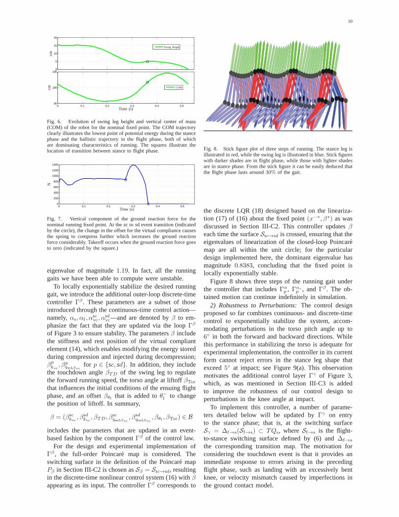
Figure 6 illustrates the evolution of the swing legheight and the vertical position of the center of massof the robot. The swing foot is over15 cm abovethe ground at its peak to offer good ground clearancefor hard impacts. During the stance phase, the COMundergoes an asymmetric motion with the lowest pointof potential energy being around52% into the stancephase. During the flight phase, the COM has a ballistictrajectory. As noted in (McMahon and Cheng, 1990)and (Holmes et al., 2006), both these aspects of COMmotion are dominant characteristics of running. Finally,Figure 7 illustrates the vertical component of the groundreaction force. Immediately upon impact, during thestance-compression phase, there is a peak in the groundreaction force due to the spring compressing rapidly onimpact. During most of the stance-compression phase,the force is fairly constant. On transition to stance-decompression phase, the energy injection causes theforce to rapidly first increase and then go to zero at whichpoint stance to flight transition occurs.

E. Parameter Update Strategies

1) Exponential Stability:To analyze the stability ofthe running gait obtained in Section IV-D in closed loopwith the continuous-time controllers (12), we employ themethod of Poincare. LetSsc→sd be the Poincare section.Then, the stability properties of the periodic runningorbit can be captured by the stability properties of thecorresponding fixed point of the restricted Poincare mapρ : Ssc→sd ∩ Zαs,αs

c→ Ssc→sd ∩ Zαs,αs

c; see (Morris

and Grizzle, 2005, 2009). Numerical computations of theeigenvalues of the linearization of the restricted Poincaremap about the fixed point of interest reveals that thecorresponding running gait is unstable with a dominant

10

0

5

10

15

20

0 0.1 0.2 0.3 0.4 0.595

100

105

Time (s)

cmcm

Swing Height

COM

Fig. 6. Evolution of swing leg height and vertical center of mass(COM) of the robot for the nominal fixed point. The COM trajectoryclearly illustrates the lowest point of potential energy during the stancephase and the ballistic trajectory in the flight phase, both of whichare dominating characteristics of running. The squares illustrate thelocation of transition between stance to flight phase.

0 0.1 0.2 0.3 0.4 0.50

200

400

600

800

1000

1200

1400

Time (s)

N

Fig. 7. Vertical component of the ground reaction force for thenominal running fixed point. At thesc to sd event transition (indicatedby the circle), the change in the offset for the virtual compliance causesthe spring to compress further which increases the ground reactionforce considerably. Takeoff occurs when the ground reaction force goesto zero (indicated by the square.)

eigenvalue of magnitude1.19. In fact, all the runninggaits we have been able to compute were unstable.

To locally exponentially stabilize the desired runninggait, we introduce the additional outer-loop discrete-timecontroller Γβ . These parameters are a subset of thoseintroduced through the continuous-time control action—namely,αs, αf , α

scvc, α

sdvc—and are denoted byβ to em-

phasize the fact that they are updated via the loopΓβ

of Figure 3 to ensure stability. The parametersβ includethe stiffness and rest position of the virtual compliantelement (14), which enables modifying the energy storedduring compression and injected during decompression;βpkvc

, βpqmLSvc

for p ∈ {sc, sd}. In addition, they includethe touchdown angleβTD of the swing leg to regulatethe forward running speed, the torso angle at liftoffβTor

that influences the initial conditions of the ensuing flightphase, and an offsetβθf that is added toθ−f to changethe position of liftoff. In summary,

β = (βsckvc

, βsdkvc

, βTD, βscqmLSvc

, βsdqmLSvc

, βθf , βTor) ∈ B

includes the parameters that are updated in an event-based fashion by the componentΓβ of the control law.

For the design and experimental implementation ofΓβ , the full-order Poincare map is considered. Theswitching surface in the definition of the Poincare mapPβ in Section III-C2 is chosen asSβ = Ssc→sd, resultingin the discrete-time nonlinear control system (16) withβappearing as its input. The controllerΓβ corresponds to

Fig. 8. Stick figure plot of three steps of running. The stanceleg isillustrated in red, while the swing leg is illustrated in blue. Stick figureswith darker shades are in flight phase, while those with lighter shadesare in stance phase. From the stick figure it can be easily deduced thatthe flight phase lasts around30% of the gait.

the discrete LQR (18) designed based on the lineariza-tion (17) of (16) about the fixed point(x−∗, β∗) as wasdiscussed in Section III-C2. This controller updatesβeach time the surfaceSsc→sd is crossed, ensuring that theeigenvalues of linearization of the closed-loop Poincaremap are all within the unit circle; for the particulardesign implemented here, the dominant eigenvalue hasmagnitude0.8383, concluding that the fixed point islocally exponentially stable.

Figure 8 shows three steps of the running gait underthe controller that includesΓα

p , Γαcp , andΓβ . The ob-

tained motion can continue indefinitely in simulation.2) Robustness to Perturbations:The control design

proposed so far combines continuous- and discrete-timecontrol to exponentially stabilize the system, accom-modating perturbations in the torso pitch angle up to6◦ in both the forward and backward directions. Whilethis performance in stabilizing the torso is adequate forexperimental implementation, the controller in its currentform cannot reject errors in the stance leg shape thatexceed5◦ at impact; see Figure 9(a). This observationmotivates the additional control layerΓγ of Figure 3,which, as was mentioned in Section III-C3 is addedto improve the robustness of our control design toperturbations in the knee angle at impact.

To implement this controller, a number of parame-ters detailed below will be updated byΓγ on entryto the stance phase; that is, at the switching surfaceSγ = ∆f→s(Sf→s) ⊂ TQs, whereSf→s is the flight-to-stance switching surface defined by (6) and∆f→s

the corresponding transition map. The motivation forconsidering the touchdown event is that it provides animmediate response to errors arising in the precedingflight phase, such as landing with an excessively bentknee, or velocity mismatch caused by imperfections inthe ground contact model.

11

0 0.2 0.4 0.6 0.8 1 1.2 1.4 1.6

0

10

20

30

replacements

Time (s)

deg

NominalWithout Γγ

(a)

0 0.2 0.4 0.6 0.8 1 1.2 1.4 1.6

0

10

20

30

Time (s)

deg

NominalWithout Γγ

With Γγ

(b)

Fig. 9. Three step simulation of a5◦ perturbation in the impact valueof the leg shape. (a) Perturbation withoutΓγ outer-loop controller,(b) Perturbation withΓγ outer-loop controller. The nominal (noperturbation) plot is shown for comparision. The squares on the plotsindicate locations at which the controller transitions from stance toflight phase.

We continue our discussion on this additional controlcomponentΓγ by providing some intuition. First notethat, to produce the same leg force, the compressionrequired in a segmented revolute-knee leg with jointcompliance is larger than that required in a prismaticleg. This phenomenon was observed in (Rummel andSeyfarth, 2008), and, in the context of MABEL, impliesthat the stiffness of the virtual compliant element shouldbe modified—i.e., increased—to prevent the leg fromexcessively bending to develop sufficient force for sup-porting the weight of the robot. Furthermore, the swingleg may have to contract additionally to ensure sufficientground clearance in the presence of shorter stance leglengths. To accommodate these requirements, the virtualcompliance stiffness,γsc

kvc, as well as the knee angle of

the swing legγLSswwill be updated according to

γsckvc

=

{

Kkscvc(qs+LSst

− qs+∗

LSst), qs+LSst

− qs+∗

LSst> 0

0, otherwise

γLSsw=

{

KLSsw(qs+LSst

− qs+∗

LSst), qs+LSst

− qs+∗

LSst> 0

0, otherwise(25)

where qs+LSstdenotes the stance leg shape angle right

after touchdown,qs+∗

LSstits nominal value. The gains

Kkscvc,KLSsw

are tuned through simulations, and theirvalues are provided in Table I.

An additional corrective action embedded inΓγ re-gards the regulation of the forward running speed. Todo this, Γγ updates a parameterγTor, which shapesthe virtual holonomic constraint imposed on the torsomotion at the beginning of stance based on the differencebetween the current forward speed and its nominal value.This allows leaning the torso forward to increase speed,or backward to decrease speed, and is implemented

TABLE IGAIN PARAMETERS FORΓγ CONTROLLER.

Gain parameter ValueKksc

vc0.46

KLSsw1.5

K+Tor

0.16K−

Tor0.31

Kδsc→sd−0.37

through the prescription

γTor =

{

K+Tor(p

h,s+

hip−p

h,s+∗

hip), (ph,s+

hip−p

h,s+∗

hip) > 0

K−

Tor(ph,s+

hip−p

h,s+∗

hip), otherwise,

(26)whereph,s+hip is the horizontal speed of the hip at impact

with the ground,ph,s+∗

hip its nominal value, and gainsK+

Tor,K−

Tor are provided in Table I. As speed increases,the energy injected during the stance-decompressionphase decreases because the time spent in this phasedecreases with increasing speed. To account for this, thecontroller Γγ will update one more parameter, namelyγδsc→sd , that modifies the location of transition fromstance-compression to stance-decompression to increaseor decrease the period over which energy is injectedin the stance-decompression phase. This is achievedthrough

γδsc→sd =

{

Kδsc→sd(ph,s+

hip−p

h,s+∗

hip), (ph,s+

hip−p

h,s+∗

hip) > 0

0, otherwise(27)

where ph,s+hip and ph,s+∗

hip have the same meaning as in(26) andKδsc→sd is provided in Table I. In summary,

γ = (γsckvc

, γTor, γLSsw, γδsc→sd) ∈ G

includes the parameters that are updated in an event-based fashion by the componentΓγ of the control law.

Under the influence ofΓγ , the robustness to perturba-tions is increased and, as shown in Figure 9(b), perturba-tions up to5◦ in the impact leg shape angle (knee beingbent an additional10◦) can be rejected. The stabilityof the closed-loop system can be analyzed through theeigenvalues of the linearization of the Poincare mapPγ

introduced in Section III-C3; more details can be foundin Appendix B where it is shown that the linearizedPoincare map has a dominant eigenvalue of magnitude0.6072 indicating that the closed-loop system with theadditional componentΓγ is locally exponentially stable.

Remark 2: Note that the controllersΓα,Γαc ,Γβ havebeen designed through rigorous control synthesis ap-proaches, whereas the design of the outer most controlloop, Γγ , has been based on heuristics. It is noted thatthe controllersΓα,Γαc ,Γβ achieve stable running insimulations on the design model. The controllerΓγ aidsin the experimental validation of running by increasingthe closed-loop system’s robustness to perturbations inthe knee angle at impact and to imperfections in theground contact model. Section V-D provides additionalcomments in this regard.

12

TABLE IISTIFFNESS CONSTANTS FOR VARIOUS SOURCES OF COMPLIANCE.

Source of compliance Stiffness valuekBsp 3.17kcable 2.46k∗vc 1.66kvc 5.08

F. Preparing for Experimental Deployment

One aspect that needs to be incorporated in the controldesign prior to experimental deployment on MABEL iscable stretch. In the leg shape coordinates, cable stretchreaches a peak value of almost15◦ just prior to lift-off,which, given that the nominal peak leg shape is around25◦ (see Figure 4), amounts for over60% of motionin the knee, thus further amplifying knee bending. Toaccount for this issue, the nominal controller designwill be modified. In more detail, the compliance dueto cable stretch will be modeled as a spring-dampersystem placed in series with the physical spring (Bspring)and the motor leg shape actuator in the transmissionmechanism. Then, active force control on the stance legcan be used to modify the virtual compliancekvc so thatthe compliance due to the cable stretchkcable togetherwith kvc has the value of the effective compliancek∗vcobtained through the optimization procedure detailed inSection IV-D; i.e.,

1

kcable+

1

kvc=

1

k∗vc. (28)

With this modification, the effective compliance of theleg is now the same as that without cable stretch, i.e.,cable stretch has been accounted for by the controldesign. Table II provides the values for the variouscompliances discussed in this section.

This modified running controller is next validated onthe detailed model as mentioned in Section II-F and isready for experimental deployment.

V. RUNNING EXPERIMENTS

This section documents experimental implementationsof the running controller developed in Sections III, IV.To illustrate the power and limitations of the proposedmethod, three experiments are presented. The first ex-periment details the execution of a transition controllerthat transitions from walking to running, the secondexperiment details a running experiment, and finally thethird experiment details the transition from running towalking. Videos of the running experiments are availableon YouTube (Sreenath et al., 2011a,c).

A. Exp. 1: Two-step Transition from Walking to Running

Running on MABEL can be implemented by transi-tioning from walking. As in (Westervelt et al., 2003), totransition from walking to running the controller modi-fies the virtual constraints corresponding to a walkinggait so that, by the end of a walking step, they are

closer to the virtual constraints of the targeted runninggait. Instead of a one-step transition from walking torunning as was done in (Morris et al., 2006), a two-steptransition is implemented to enable a smoother transitionby preventing rapid torso motions on MABEL. This isespecially important for gaits where the final and initialvalues of the torso virtual constraint differ significantlybetween the walking and running fixed points, respec-tively. A walking-to-running transition then consists ofthe following: (a) A transition from the nominal walkinggait to a transition-walk-step, followed by (b) a transitionfrom the transition-walk-step to a transition-run-step, andfinally (c) a transition from the transition-run-step tothe nominal running gait. Figure 10(a) illustrates plotsof various variables for the transition from walking torunning. The walking and running sections are clearlymarked along with the two transition steps.

B. Exp. 2: Running with Point Feet

Initial experiments on MABEL failed to achievesteady-state running due to foot slippage and the con-troller’s poor performance in regulating forward speed.This is a consequence of imperfections in the groundcontact model used in the controller design. To addressthese issues, the point feet were replaced with passivefeet with shoes to provide a larger surface area for trac-tion, thereby preventing slipping. With this configuration,successful running was achieved—see Appendix A formore details on these experiments—suggesting certainmodifications to the running controller of Sections III,IV in order to achieve running on point feet.

In more detail, to regulate the forward speed, theγ-parameter corresponding to the virtual compliance ismodified as in (31) and saturation in theβ-parametercorresponding to the touchdown angle is introducedas in (32); see Appendix A. Finally, theγ-parameterthat modifies the location of the stance-compression tostance-decompression phase will also be saturated as afunction of the speed as,

γsatδsc→sd

=

0.2, 0 ≤ ph,avghip < 2

0.25, 2 ≤ ph,avghip < 2.5

0.35, 2.5 ≤ ph,avghip

. (29)

At high speeds, the time spent in the stance-decompression phase decreases, which results in lessenergy being injected and smaller push-offs. With theabove modification, a well defined flight phase is main-tained even at fast running motions.

Next, to prevent the stance-decompression phase fromcausing a lift-off with a high velocity, the stance-decompression to flight phase switching surface is mod-ified as follows

Sexpsd→f := Ssd→f ∩ {xs ∈ TQs | pvhip > pv,s−∗

hip }. (30)

In addition, during the stance-decompression phase, thetorso is pushed back in a similar manner as in the runningwith feet experiment. Finally, during the flight phase, the

13

Walking Running

160

180

200

220

0

10

20

30

40

50

0

10

20

30

40

50

−25

−20

−15

−10

−5

0

5

−15

−10

−5

0

5

10

15

Nm

10 10.5 11 11.5 12 12.5 13 13.5 14 14.5−30

−20

−10

0

10

20

30

Time (s)

Nm

Transition Walk StepTransition Run Step

deg

deg

deg

deg

Phase

qLA

qLS

Stance

Stance

Stance

Stance

Stance

Swing

Swing

Swing

Swing

Swing

qBsp

qTor

umLA

umLS

(a)

WalkingRunning

160

180

200

220

0

10

20

30

40

50

0

10

20

30

40

50

−25

−20

−15

−10

−5

0

5

−15

−10

−5

0

5

10

15

Nm

11.5 12 12.5 13 13.5 14 14.5 15 15.5−30

−20

−10

0

10

20

30

Time (s)

Nm

Transition Walk Step

deg

deg

deg

deg

Phase

qLA

qLS

Stance

Stance

Stance

Stance

Stance

Swing

Swing

Swing

Swing

Swing

qBsp

qTor

umLA

umLS

(b)

Fig. 10. Experimental plots of the internal phase variable, joint angles, and motor torques for (a) transition from walking to running (Exp. 1)and (b) transition from running to walking (Exp. 3). The internal phase variable of the controller indicates the walkingand running parts ofthe gait, with the thicker plots indicating the transition steps. Note that, for transition to running there are two transition steps - one duringwalking and the other during running, while for transition to walking there is one transition step during walking. Also note that the peak springcompression for running is around2.5 times that for walking.

adaptive correction polynomials, as used for the runningwith feet experiment, are deployed. Both these changescounteract the effect of unmodeled cable stretch in theleg angle direction.

With these changes to the controller developed inSections III, IV, the running experiment is carried outas follows. First, walking is initiated on MABEL usingthe walking controller developed in (Sreenath et al.,2011b). Next, the walking to running transition con-troller, presented in Section V-A, is executed. Finally, ontransition to running, the running controller is executed.The running controller induced stable running at anaverage speed of1.95 m/s, and a peak speed of3.06m/s.113 running steps were obtained and the experimentterminated when the power to the robot was cut off. At2 m/s, the average stance and flight times of233 msand 126 ms are obtained respectively, corresponding to

a flight phase that is35% of the gait. At 3 m/s, theaverage stance and flight times of195 ms and123 msare obtained respectively, corresponding to a flight phasethat is 39% of the gait. An estimated ground clearanceof 3− 4 inches (7.5− 10 cm) is obtained. The specificcost of mechanical transport (cmt), defined in (Collinsand Ruina, 2005), was computed to be1.07.

Figure 11(a) depicts snapshots at100 ms intervals of atypical running step. Figure 12(a) depicts the mean jointangles, and motor torques temporally normalized overtime, for 50 consecutive steps of running.

The outer-loop event based controller parameters aredepicted in Figures 13(a), 14(a). Considerable variationin the speed is observed. In particular, when the speedexceeds2.5 m/s, large changes in the touch down an-gle, βTD, and theγ-parameter that affects the transi-tion from stance-compression to stance-decompression,

14

41.8 42 42.2 42.4 42.6 42.8 43 43.2

0

2

4

6

8

10

12

replacements

Time (s)

deg

Cable StretchScaled Spring

Fig. 15. Absolute value of leg shape cable stretch and springcompression for the stance leg for the running with point feet(Exp. 2.).Both variables are scaled to be in the leg shape coordinates.As isseen, cable stretch contributes as much as the spring to the compliancepresent in the system. This was hinted at in Table II.

γδsc→sd causes the speed to dramatically drop to under1m/s. All this is autonomously handled by the controllerwith no manual intervention. The ability of the controllerto recover from slow speeds below1 m/s, and highspeeds above2.5 m/s illustrates a good robustness to im-perfections in the ground contact model. The controller isalso able to account for significant cable stretch (shownin Figure 15.)

C. Exp. 3: One-step Transition from Running to Walking

This section briefly describes the controller used totransition from running to walking. To realize suchtransitions, the running controller is switched to a walk-ing controller that creates virtual compliance throughactive force control on the stance leg shape motor. Thiswalking controller essentially treats a running-to-walkingtransition as a large step-down, similarly to what wasdone in (Park et al., 2012) for walking gaits. Figure 10(b)illustrates plots of various variables for the transitionfrom running to walking. The running and walkingsections are clearly marked along with the transition step.Note that transition from running to walking is achievedin a single step.

D. Discussion of the Experiments

The experimental implementation of running motionson MABEL revealed a number of interesting observa-tions regarding the robot and the proposed controller.First, it was observed that the robot runs faster inexperiments than what simulations predict based on thedeveloped models. This behavior is similar to whatwas observed in walking experiments with MABEL(Sreenath et al., 2011b), and is attributed to the inevitableinaccuracies associated with the ground contact model.While in (Sreenath et al., 2011b, Sec. VII-B) we suggestvarious ways of modeling the ground impact demonstrat-ing that impact scaling can account for speed differencesin walking, it is not clear how the parameters of thecompliant ground model can be selected to improve theaccuracy of the simulations in the case of running.

Another source of inaccuracy is the assumption ofplanar motion that underlies the model based on whichthe controller is derived. Clearly, the support boom in the

experimental setup constraints the robot’s hip to moveon the surface of a sphere and not in sagittal plane.Furthermore, the boom affects the weight distribution sothat the robot weighs10%—approximately7 Kg—morewhen supported on the inner leg than when supportedon the outer leg. In running, this asymmetry resultsin harder impacts on the inside leg causing its kneeto bend more during the corresponding stance phase.As a consequence, the outer-loop component of thecontroller tends to overcompensate in the following step;notice the pronounced step-to-step oscillations in thevirtual compliance in Figure 14(a). To account for thisphenomenon, the controller can be modified so thatthe virtual compliance is10% stiffer on the inside leg.Moreover, for smoother running motions, the outer-loopcontrollers can perform separate step-to-step updatesover two steps.

As a final remark, note that the proposed con-troller combines formal control synthesis procedureswith heuristics to experimentally realize running onMABEL. The inner-loop control components—namely,Γα, Γαc , and Γβ—are designed through systematiccontrol methods to meet certain specifications such ashybrid invariance and local exponential stability. Onthe contrary, the outer-loop event-based controllerΓγ

is based on certain intuitive observations aiming toenhance the robustness of the controller to perturbationsin the knee angle at impact and to imperfections inthe ground contact model. To minimize the relianceof the controller on heuristics, the softening effect ofthe spring for large knee angles can be incorporatedin the continuous-time control component by suitablymodifying the virtual compliance (14) to include thenonlinear relation between the knee bending angle andthe developed leg force as observed in (Rummel andSeyfarth, 2008). Similarly the effect of cable stretchcan also be included in (14). With these modifications,the outer-loop componentsΓγ could be removed fromthe design andΓβ would be sufficient to ensuring bothexponential stability and robustness.

VI. CONCLUSION

MABEL contains springs in its drivetrain for thepurposes of enhancing agility and robustness of dynamiclocomotion. This paper has presented a model-basedcontrol design method to realize the potential of thesprings. Experiments have been performed to illustrateand confirm important aspects of the feedback design.

The controller is based on the hybrid zero dynamicsintroduced in (Poulakakis and Grizzle, 2009b) and fur-ther developed and deployed experimentally in (Sreenathet al., 2011b). An important modification was the de-liberate inclusion of actuation in the zero dynamicsduring the stance phase of running, which enabled activeforce control of the stance knee. Specifically, a virtualcompliant element was created to dynamically vary theeffective leg compliance during stance. An outer-loop

15

(a) (b)

Fig. 11. Snapshots of a typical running step for (a) running with point feet, and (b) running with passive feet, are shown at intervals of100ms. The snapshots progress temporally from left to right and from top to bottom. Videos of the experiments are available on YouTube (Sreenathet al., 2011a,c).

160

180

200

220

−10

0

10

20

30

40

50

0

10

20

30

40

50

−30

−20

−10

0

10

−15

−10

−5

0

5

10

15

0 10 20 30 40 50 60 70 80 90 100−30

−20

−10

0

10

20

30

deg

deg

deg

deg

% gait

qLA

qLS

Stance

Stance

Stance

Stance

Swing

Swing

Swing

Swing

qBspst

qTor

umLA

umLS

Nm

Nm

(a)

160

180

200

220

−10

0

10

20

30

40

50

0

10

20

30

40

50

−30

−20

−10

0

10

−15

−10

−5

0

5

10

15

0 10 20 30 40 50 60 70 80 90 100−30

−20

−10

0

10

20

30

deg

deg

deg

deg

% gait

qLA

qLS

Stance

Stance

Stance

Stance

Swing

Swing

Swing

Swing

qBspst

qTor

umLA

umLS

Nm

Nm

(b)

Fig. 12. Ensemble plots of joint angles and motor torques of thestance and swing legs for50 consecutive steps of (a) running with pointfeet, and (b) running with passive feet. The solid lines represent the mean recorded joint angle waveforms, while the dotted lines indicate theupper and lower quartiles over the running steps. The curveswere temporally normalized from initial touchdown (0%) to subsequent touchdown(100%).

16

−3

−2.5

−2

−1.5

−1

−0.5

0

0.5

1

deg

−3

−2

−1

0

1

2

3

4

Step No.−0.05

0

0.05

0.1

0.15

20 30 40 50 60−10

−5

0

5x 10

−3

Step No.

m

20 30 40 50 60−4

−3

−2

−1

0

1

2

3

4

5

Step No.

deg

scsd

scsd

βqmLSvcβTD βkvc

βθf βTor

(a)

−3

−2.5

−2

−1.5

−1

−0.5

0

0.5

1

deg

−3

−2

−1

0

1

2

3

4

Step No.−0.05

0

0.05

0.1

0.15

20 30 40 50 60−10

−5

0

5x 10

−3

Step No.

m

20 30 40 50 60−4

−3

−2

−1

0

1

2

3

4

5

Step No.

deg

scsd

scsd

βqmLSvcβTD βkvc

βθf βTor

(b)

Fig. 13. Parameter plots for50 consecutive steps for the outer-loop event-based controller,Γβ , for (a) running with point feet and (b) runningwith passive feet.sc, sd refer to the values of the correspondingβ-parameters in the stance-compression and stance-decompression subphasesrespectively.

0

2

4

6

8

10

deg

−0.4

−0.35

−0.3

−0.25

−0.2

−0.15

−0.1

−0.05

0

20 30 40 50 60−0.5

−0.4

−0.3

−0.2

−0.1

0

0.1

Step No.

deg

20 30 40 50 60−8

−6

−4

−2

0

2

4

Step No.

scsd

γLSswγδsc→sd

γkvcγTor

(a)

0

2

4

6

8

10

deg

−0.4

−0.35

−0.3

−0.25

−0.2

−0.15

−0.1

−0.05

0

20 30 40 50 60−0.5

−0.4

−0.3

−0.2

−0.1

0

0.1

Step No.

deg

20 30 40 50 60−8

−6

−4

−2

0

2

4

Step No.

scsd

γLSswγδsc→sd

γkvcγTor

(b)

Fig. 14. Parameter plots for50 consecutive steps for the nonlinear outer-loop controllerfor increasing robustness to perturbations ,Γγ , for (a)running with point feet and (b) running with passive feet.sc, sd refer to the values of the correspondingγ-parameters in the stance-compressionand stance-decompression subphases respectively.

event-based controller was designed to exponentiallystabilize the periodic running gait. An additional outer-loop event-based controller was designed to improve therobustness of the periodic running gait to perturbationsin the knee angle at impact and to imperfections in theground contact model.

The running controller has been experimentally de-ployed and stable running has been successfully demon-strated on MABEL, both with passive feet and withpoint feet. The achieved running is dynamic and life-like, exhibiting flight phases of significant duration andhigh ground clearance. For running with point feet, thedeveloped controller resulted in a kneed-biped runningrecord of3.06 m/s (10.9 kph or 6.8 mph).

Acknowledgments

The authors are grateful to A. Ramezani for his experthelp with the experiments. K. Sreenath acknowledges L.

McCauley for suggesting the experiments with nontrivialfeet, and B. Morris is thanked for his advice - “Go big,or go home,” which helped us to focus on multiple stepsof running, and for his contributions to the theoreticalunderpinnings of our work, as cited in the text. J.Konscol is thanked for his weekly visits to the lab and forsharing his engineering experience, which contributedinvaluably to the robustness of the electronic setup of thetestbed. G. Buche is thanked for his many contributionsto the design of the electronics, power supply, and safetyinterlock systems. Last but not least, we are deeplyindebted to J. Hurst for designing MABEL. We hopethat this paper has once again confirmed many of hisexpectations for the robot.

REFERENCES

Ahmadi, M. and Buehler, M. (1997). Stable Control of aSimulated One-Legged Running Robot with Hip andLeg Compliance. 13(1):96–104.

17

Ahmadi, M. and Buehler, M. (2006). Controlled passivedynamic running experiments with the arl-monopodii. IEEE Transactions on Robotics, 22(5):974–986.

Alexander, R. (1990). Three uses for springs in leggedlocomotion. The International Journal of RoboticsResearch, 9(2):53–61.

Ames, A. D., Gregg, R. D., Wendel, E. D. B., andSastry, S. (2006). Towards the geometric reduction ofcontrolled three-dimensional bipedal robotic walkers.In 3rd Workshop on Lagrangian and HamiltonianMethods for Nonlinear Control, pages 183–196.

Andrews, B., Miller, B., Schmitt, J., and Clark, J. E.(2011). Running over unknown rough terrain with aone-legged planar robot.Bioinspiration & Biomimet-ics, 6(2):1–15.

Chevallereau, C., Abba, G., Aoustin, Y., Plestan, F.,Westervelt, E. R., de Wit, C. C., and Grizzle, J. W.(2003). Rabbit: a testbed for advanced control theory.IEEE Control Systems Magazine, 23(5):57–79.

Chevallereau, C., Grizzle, J. W., and Shih, C.-L. (2009).Asymptotically stable walking of a five-link under-actuated 3d bipedal robot.IEEE Transactions onRobotics, 25(1):37–50.

Cho, B.-K., Park, S.-S., and ho Oh, J. (2009). Controllersfor running in the humanoid robot, HUBO. InIEEE-RAS International Conference on Humanoid Robots,pages 385–390, Paris, France.

Collins, S. H. and Ruina, A. (2005). A bipedal walkingrobot with efficient and human-like gait. InIEEE In-ternational Conference on Robotics and Automation,pages 1983–1988, Barcelona, Spain.

Daley, M. A. and Biewener, A. A. (2006). Running overrough terrain reveals limb control for intrinsic stability.Proceedings of the National Academy of Sciences ofthe United States of America, 103(42):15681–15686.

Daley, M. A., Usherwood, J. R., Felix, G., and Biewener,A. A. (2006). Running over rough terrain: guinea fowlmaintain dynamic stability despite a large unexpectedchange in substrate height.The Journal of Experimen-tal Biology, 209:171–187.

Ferris, D. P. and Farley, C. T. (1997). Interaction of legstiffness and surface stiffness during human hopping.Journal of applied physiology, 82:15–22.

Ferris, D. P., Louie, M., and Farley, C. T. (1998).Running in the real world: adjusting stiffness fordifferent surfaces.Proceedings of The Royal Society,265(1400):989–994.

Ghigliazza, R. M., Altendorfer, R., Holmes, P., andKoditschek, D. E. (2003). A Simply Stabilized Run-ning Model. SIAM Journal of Applied DynamicalSystems, 2(2):187–218.

Gregg, R. D. and Spong, M. W. (2010). Reduction-based control of three-dimensional bipedal walkingrobots. The International Journal of Robotics Re-search, 29(6):680–702.

Grizzle, J. W., Hurst, J., Morris, B., Park, H.-W., andSreenath, K. (2009). MABEL, a new robotic bipedalwalker and runner. InAmerican Control Conference,

pages 2030–2036, Saint Louis, MO, USA.Hirose, M. and Ogawa, K. (2007). Honda humanoid

robots development.Philosophical Transactions ofThe Royal Society A, 365(1850):11–19.

Holmes, P., Full, R. J., Koditschek, D., and Gucken-heimer, J. (2006). The dynamics of legged locomo-tion: Models, analyses, and challenges.SIAM Review,48(2):207–304.

Hurmuzlu, Y. and Chang, T. (1992). Rigid body col-lisions of a special class of planar kinematic chains.IEEE Transactions on Systems, Man and Cybernetics,22(5):964–71.

Hurst, J. W. (2008). The Role and Implementationof Compliance in Legged Locomotion. PhD thesis,Carnegie Mellon University.

Hurst, J. W. and Rizzi, A. A. (2008). Series compliancefor an efficient running gait. IEEE Robotics &Automation Magazine, 15(3):42–51.

Isidori, A. (1995).Nonlinear Control Systems. Springer-Verlag, Berlin, third edition.

Kajita, S., Kaneko, K., and Morisawa, M. (2007). Zmp-based biped running enhanced by toe springs. InIEEEInternational Conference on Robotics and Automa-tion, pages 3963–3969, Roma, Italy.

Kajita, S., Nagasaki, T., Kaneko, K., Yokoi, K., andTanie, K. (2005). A running controller of humanoidbiped hrp-2lr. InIEEE International Conference onRobotics and Automation, pages 616–622, Barcelona,Spain.

Koechling, J. C. (1989).The limits of running speed:Experiments with a legged robot. PhD thesis, CarnegieMellon University, Pittsburgh, PA.

Koepl, D., Kemper, K., and Hurst, J. (2010). Forcecontrol for spring-mass walking and running. InIEEE/ASME International Conference on AdvancedIntelligent Mechatronics, pages 639–644, Montreal,Canada.

McGeer, T. (1990). Passive bipedal running.Proceedingsof the Royal Society of London, 240(1297):107–34.

McMahon, T. A. and Cheng, G. C. (1990). The mechan-ics of running: How does stiffness couple with speed?Journal of Biomechanics, 23(1):65–78.

McMahon, T. A., Valiant, G., and Frederick, E. C.(1987). Groucho running.Journal of Applied Physi-ology, 62(6):2326–37.

Morris, B. and Grizzle, J. W. (2005). A restrictedPoincare map for determining exponentially stableperiodic orbits in systems with impulse effects: Ap-plication to bipedal robots. InIEEE Conference onDecision and Control, pages 4199–206, Seville, Spain.

Morris, B. J. and Grizzle, J. W. (2009). Hybrid invari-ant manifolds in systems with impulse effects withapplication to periodic locomotion in bipedal robots.IEEE Transactions on Automatic Control, 54(8):1751– 1764.

Morris, B. J., Westervelt, E. R., Chevallereau, C., Buche,G., and Grizzle, J. W. (2006).Achieving BipedalRunning with RABBIT: Six Steps Toward Infinity,

18

volume 340 ofLecture Notes in Control and Infor-mation Sciences, pages 277–297. Springer Berlin /Heidelberg.

Nagasaka, K., Kuroki, Y., Itoh, S., and Yamaguchci,J. (2004). Integrated motion control for walking,jumping and running on a small bipedal entertainmentrobot. In IEEE International Conference on Roboticsand Automation, pages 3189–3194, New Orleans, LA.

Park, H.-W., Sreenath, K., Hurst, J. W., and Grizzle,J. W. (2011). Identification of a bipedal robot with acompliant drivetrain: Parameter estimation for controldesign.Control Systems Magazine, 31(2):63–88.

Park, H.-W., Sreenath, K., Ramezani, A., and Grizzle,J. W. (submitted, 2012). Switching control designfor accommodating large step-down disturbances inbipedal robot walking. InIEEE International Confer-ence on Robotics and Automation.

Poulakakis, I. (2008). Stabilizing Monopedal RobotRunning: Reduction-by-Feedback and Compliant Hy-brid Zero Dynamics. PhD thesis, The University ofMichigan.

Poulakakis, I. and Grizzle, J. W. (2009a). Modeling andcontrol of the monopedal robot thumper. InIEEE In-ternational Conference on Robotics and Automation,pages 3327–3334, Kobe, Japan.

Poulakakis, I. and Grizzle, J. W. (2009b). The springloaded inverted pendulum as the hybrid zero dynamicsof an asymmetric hopper. IEEE Transactions onAutomatic Control, 54(8):1779–1793.

Raibert, M. H. (1986).Legged Robots that Balance. MITPress, Cambridge, MA.

Rummel, J. and Seyfarth, A. (2008). Stable running withsegmented legs.The International Journal of RoboticsResearch, 27(8):919–934.

Sayyad, A., Seth, B., and Seshu, P. (2007). Single-leggedHopping Robotics Research.Robotica, 25:587–613.

Spong, M. W. (1999). Passivity based control of thecompass gait biped. InIFAC World Congress.

Sreenath, K. (2011). Feedback Control of a BipedalWalker and Runner with Compliance. PhD thesis, TheUniversity of Michigan, Ann Arbor, MI.

Sreenath, K., Park, H.-W., and Grizzle, J. W. (2011a).MABEL runs free! YouTube video.

Sreenath, K., Park, H.-W., Poulakakis, I., and Griz-zle, J. W. (2011b). Compliant hybrid zero dynam-ics controller for achieving stable, efficient and fastbipedal walking on MABEL.International Journal ofRobotics Research, 30(9):1170–1193.

Sreenath, K., Park, H.-W., Ramezani, A., and Grizzle,J. W. (2011c). MABEL runs in style. YouTube video.

Tajima, R., Honda, D., and Suga, K. (2009). Fast runningexperiments involving a humanoid robot. InIEEE In-ternational Conference on Robotics and Automation,pages 1571–1576, Kobe, Japan.

Westervelt, E. R., Grizzle, J. W., Chevallereau, C., Choi,J. H., and Morris, B. (2007). Feedback Controlof Dynamic Bipedal Robot Locomotion. Taylor &Francis/CRC Press, Boca Raton, FL.

Westervelt, E. R., Grizzle, J. W., and de Wit, C. C.(2003). Switching and PI control of walking motionsof planar biped walkers.IEEE Transactions on Auto-matic Control, 48(2):308–312.

APPENDIX ARUNNING WITH PASSIVE FEET

To avoid slipping, MABEL’s original shins terminat-ing at point feet were replaced with shins terminatingin passive feet enclosed in regular running shoes thatprovide a larger surface area for better traction. Withthe addition of the passive feet, the model developedin Section II is no longer valid due to (a) the differentinertia properties between the two designs, and (b) thedifferent toe-ground interactions, which, in the case ofshoes, result in softer impacts due to the rolling contactwith the ground. To accommodate these differences, anumber of modifications will be made in the controller.

Modifications to regulate speed:At faster speeds, thetime spent in the stance-decompression phase decreases.As a result, the effective energy injection is reduced,resulting in a lower peak apex height in flight. Tomaintain a well defined flight phase at fast speeds, anadditional parameter,γδsc→sd (see (27)), was added toΓγ to modify the location of the stance-compression tostance-decompression switching surface.

As suggested in (McGeer, 1990; McMahon andCheng, 1990), animals vary stance leg stiffness to reg-ulate running speed. Thus, there is a need for thecontroller to change the effective leg compliance asa function of speed. This is achieved by adding anadditional term∆γsc

kvcto γsc

kvccomputed in (25), where,

∆γsckvc

:=

{

−Kkscvc

√

∆ph,avghip , ∆ph,avghip > 0

0, otherwise, (31)

with, ∆ph,avghip = (ph,avghip − ph,avg∗hip ), and ph,avg∗hip , ph,avghip

being the nominal and last step average horizontal hipspeeds respectively.

Finally, to enable large touchdown angles at fasterspeeds to effectively slow down the robot and to preventlarge touchdown angles at slow speeds from causing thefoot to slip, theβ-parameters are bounded, such that,−βsat ≤ β ≤ βsat, with the saturation for theβ-parameter corresponding to touchdown,βTD, specifiedas a function of speed, as below,

βsatTD =

2◦, 0 ≤ ph,avghip < 1.2

1.5◦, 1.2 ≤ ph,avghip < 1.7

2◦, 1.7 ≤ ph,avghip < 2

2.5◦, 2 ≤ ph,avghip < 2.5

4◦, 2.5 ≤ ph,avghip

(32)

Modifications to account for the passive feet:Thesofter impacts due to the feet in the shoes result inthe spring not compressing sufficiently and cause flightphases with smaller durations and with lower ground

19

clearance. To account for the softer impacts, the nominalvirtual compliance,k∗vc, was reduced by18%.

During stance-decompression, energy injection causesthe spring to compress initially and then rapidly decom-press resulting in rapid knee extension causing push off.However, due to the geometry of the passive foot—specifically, the absence of an ankle rotation DOF—when the leg is backward at the beginning of stance-decompression, only the forward part of the shoe is incontact with the ground. This causes a significant frac-tion of the injected energy not to be translated to a pushoff; rather it rapidly affects the angle of the foot withrespect to the ground. This effect is more pronouncedwhen the spring is close to its rest position. To addressthis, the stance compression-to-decompression switchingsurface is modified to ensure that switching occurs whenthe spring is sufficiently compressed,

Sexpsc→sd := Ssc→sd∩{xs ∈ TQs | θs > θ50%, qBspst

< 20◦},(33)

where,θ50% is the value ofθs at 50% into stance.To prevent (a) slipping towards the end of stance when

the stance forces are small, (b) hyper-extension of theheavy shin, and (c) large vertical velocities at liftoff,the stance-decompression to flight switching surface ismodified as below,

Sexpsd→f := Ssd→f ∩ {xs ∈ TQs | qBspst

< 15◦,

qLSst< 2◦} ∩ {xs ∈ TQs | pvhip > pv,s−∗

hip },(34)

where,pvhip is the vertical hip velocity, andpv,s−∗

hip is thenominal liftoff vertical hip velocity.

Finally, to prevent the shoes from scuffing the groundduring leg swing, the swing leg shape virtual constraintis modified to fold the leg by an additional constantamount.

Modifications to account for unmodeled cable stretchin leg angle transmission:The running controller ac-counts for unmodeled cable stretch in the leg shapecoordinates, but not the leg angle coordinates. Duringthe stance-decompression phase, the nominal virtualconstraint specifies the torso to pitch backward. Inexperiments, the torso is sometimes driven forward tocorrect tracking errors, which results in forward pitchingduring flight causing a significant torso error on impact.To prevent this, when the torso velocity drops below athreshold, the controller for the torso pushes the torsobackward instead of enforcing the virtual constraint.

On initiation of the flight phase, the event-basedcontroller Γαc

f ensures hybrid invariance through thecorrection polynomials,hf

c as in (15), such that themodified virtual constraints smoothly join the nominalones half-way into the flight phase. During experi-ments, large errors at liftoff may cause the modifiedvirtual constraint to initially reverse the direction ofmotion, resulting in significant leg angle cable stretchand subsequent large touchdown errors. To handle this,the correction polynomials are modified such that themodified virtual constraint smoothly joins the nominal

one at an adaptively chosen location that is either50%,75%, or 95% into the flight phase, depending on the signand magnitude of the error on transition to flight.

With these modifications, the running experimentswith passive feet can be performed. The walking con-troller of (Sreenath et al., 2011b) is employed, along witha torso offset to lean the torso forward to induce stablewalking with the passive feet at1.26 m/s. The walking-to-running transition controller developed in section V-Ais used to excite running. On transition, the modifiedcontroller described above is executed to sustain runningat an average speed of1.07 m/s obtaining100 runningsteps. Figure 11(b) illustrates snapshots of a typicalrunning step. The average stance and flight times are360 ms and151 ms, respectively, i.e. flight amounts for30% of the gait. The ground clearance is approximately2 inches (5 cm) and the specific cost of mechanicaltransport (cmt) is 0.75. Figure 12(b) depicts the meanjoint angles and motor torques, normalized over time,for 50 consecutive steps of running. Figures 13(b), 14(b)illustrate theβ andγ-parameters.

APPENDIX BANALYZING STABILITY OF Γγ CONTROLLER

To analyze stability, the Poincare map is numericallycomputed. To ease computation, the sectionSγ = {xs ∈TQs | θs = θ77%} will be considered instead ofSγ ; Sγ

represents a switching surface77% into the stance phase.We can then study the eigenvalues of the Poincare mapPγ : Sγ × B × G → Sγ . Note that, while the Poincaresection Sγ is used instead ofSγ , the β, γ parametersstill continue to be updated on their respective switchingsurfacesSβ and Sγ . To define the Poincare map Pγ ,we define three maps:P 1

γ : Sγ × B × G → Sγ whichmaps a state onSγ along with β and γ to the post-impact surface, which is also the switching surfaceSγ

for the event-based controllerΓγ ; P 2γ : Sγ×B×G → Sβ

which maps a state onSγ to the stance-compression tostance-decompression transition surface, which is alsothe switching surfaceSβ for the event-based controllerΓβ ; and finally P 3

γ : Sβ × B × G → Sγ , which mapsa state onSβ back to Sγ , the Poincare section underconsideration. To further clarify this, we define,

xap[k] = P1

γ(xp[k], β[k], γ[k]) (35)

xbp[k] = P2

γ(xap[k], β[k],Γ

γ(xap[k])). (36)

Then,

xp[k + 1] = Pγ(xp[k], β[k], γ[k])

= P3γ

(

xbp[k],Γ

β(xbp[k]),Γ

γ(xap[k])

)

.(37)

Thus theγ parameters continue to be updated on theswitching surfaceSγ , while theβ parameters are updatedon the switching srufaceSβ . The switching sectionSγ

serves only to define the Poincare mapPγ . With this,the eigenvalues of the linearized Poincare map was com-puted and a dominant eigenvalue of magnitude0.6072

20

TABLE IIIGLOSSARY OF SYMBOLS.

Symbol Descriptionαp Coefficients for Bezier polynomial forp ∈ Pαcp Coefficients for correction polynomial forp ∈ P

αvc Parameter vector for the virtual compliant elementβ Parameter vector forΓβ controllerγ Parameter vector forΓγ controller

∆s→f Stance to flight impact map∆f→s Flight to stance impact mapΓαp Continuous-time controller forp ∈ P

Γβ Discrete-time controller for hybrid invarianceΓγ Discrete-time controller for robustnessBe Input matrix for unconstrained dynamicsCe Coriolis matrix for unconstrained dynamicsDe Inertia matrix for unconstrained dynamics

FNtoest

Stance toe normol ground reaction forcefs, ff Drift vector field for stance, flight dynamicsGe Gravity matrix for unconstrained dynamicsgs, gf Input vector field for stance, flight dynamicsgmLSst

Input vector field for stance motor leg shape inputH

p0 Controlled variable selection matrix forp ∈ P

hp Virtual constraints forp ∈ Phpd

Desired evolution of virtual constraints forp ∈ Phpc Correction terms for virtual constraints forp ∈ P

P = {s, f} Represents the stance, flight phase setPβ Poincare map forΓβ controllerPγ Poincare map forΓγ controller

phhip

, pvhip

Horizontal and vertical position of the hippvtoesw Vertical position of swing toeQe Unconstrained / extended configuration spaceQs Stance configuration spaceQf Flight configuration space

qe, qs, qf Generalized coordinate vector inQe, Qs, Qf

qLAst, qLAsw

Leg angle coordinate for stance, swing legqLSst

, qLSswLeg shape coordinate for stance, swing leg

qmLSst, qmLSsw

Leg angle motor angle for stance, swing legqBspst

, qBspswBspring pulley angle for stance, swing leg

qTor Torso angleSβ Poincare section forPβ

Sγ Poincare section forPγ

Ss→f Stance to flight switching surfaceSf→s Flight to stance switching surface

TQs, TQf Tangent bundle for stance, flightU Input setu Input vector

umLSstStance motor leg shape torque

u Actuators used to enforce stance virtual constraintsu∗

p Input that rendersZαp invariant forp ∈ Pxs, xf State vector for stance, flight dynamicsx−

s , x−

fPre-transition stance, flight state

x+s , x+

fPost-transition stance, flight state

yp Virtual constraints forp ∈ Pycp Virtual constraints with corrections forp ∈ PZαp Zero dynamics surface forp ∈ Pzp State on zero dynamics surface forp ∈ P

was obtained indicating that the closed-loop system stillremains exponentially stable.