eloise hamilton supervisor: dr david smyth october 2015smythd/papers/eloise's thesis.pdf ·...

Moduli spaces for singular curves

Eloise Hamilton

Supervisor: Dr David Smyth

October 2015

A thesis submitted for the degree of Bachelor of Philosophy (Science)

of the Australian National University

Declaration

Except where otherwise stated, this thesis is my own work prepared under the supervision

of Dr David Smyth.

Eloise Hamilton

Acknowledgements

Above all I would like to thank my Honours supervisor David Smyth for his guidance and

insight which kept me inspired throughout this honours year. David suggested a perfect

topic for me, provided untiring advice, ideas and encouragement, and most of all made

the learning process thoroughly enjoyable.

I would also like to thank the lecturers at the MSI who have encouraged and supported

me throughout my four years at ANU, including my mentor Jim Borger, Tim Trudgian,

Pierre Portal, Joan Licata, Griffith Ware and Dennis The.

On a more personal level my thanks as well to my fellow maths honours students Jack

Davies and Suo Jun Tan for the much-needed diversions, the shared laughs and the long

conversations over a whiteboard that we filled with flippancy more than formulas.

Thanks also to Hafiz Khusyairi and Chi-Yu Cheng who shared our office in MSI and

added fun to our long days. I am grateful to Chi-Yu for always having the patience to go

back to basics and to Hafiz for helping with the proofreading.

I am grateful as well to my housemate Rob Culling with whom I shared not only a

house but a love of maths. Thanks for the endless discussions in the stairway, and for your

help with proofreading.

And last but not least my thanks to the ANU Food Co-op Cafe for providing the

lunchtime nourishment and conviviality that sustained me during my time at ANU.

v

Contents

Acknowledgements v

Introduction 1

0.1 What is a curve? . . . . . . . . . . . . . . . . . . . . . . . . . . . . . . . . . 1

0.2 Classifying smooth projective curves . . . . . . . . . . . . . . . . . . . . . . 5

0.3 Classifying curve singularities . . . . . . . . . . . . . . . . . . . . . . . . . . 7

0.4 Classifying singular curves . . . . . . . . . . . . . . . . . . . . . . . . . . . . 7

0.5 Structure of the thesis . . . . . . . . . . . . . . . . . . . . . . . . . . . . . . 8

1 Abstract varieties and abstract curves 9

1.1 Sheaves and ringed spaces . . . . . . . . . . . . . . . . . . . . . . . . . . . . 10

1.1.1 Definitions . . . . . . . . . . . . . . . . . . . . . . . . . . . . . . . . 10

1.1.2 New k-ringed spaces from existing ones . . . . . . . . . . . . . . . . 13

1.2 Varieties . . . . . . . . . . . . . . . . . . . . . . . . . . . . . . . . . . . . . . 17

1.2.1 Affine space . . . . . . . . . . . . . . . . . . . . . . . . . . . . . . . . 18

1.2.2 Spectrum of a ring . . . . . . . . . . . . . . . . . . . . . . . . . . . . 20

1.2.3 Affine varieties and abstract varieties . . . . . . . . . . . . . . . . . . 25

1.3 Varieties and their properties . . . . . . . . . . . . . . . . . . . . . . . . . . 28

1.3.1 Subvarieties and product varieties . . . . . . . . . . . . . . . . . . . 28

1.3.2 Global properties . . . . . . . . . . . . . . . . . . . . . . . . . . . . . 33

1.3.3 Local properties . . . . . . . . . . . . . . . . . . . . . . . . . . . . . 36

1.4 Normalisation and resolution of singularities . . . . . . . . . . . . . . . . . . 38

1.4.1 Normalisation . . . . . . . . . . . . . . . . . . . . . . . . . . . . . . . 39

1.4.2 Curves . . . . . . . . . . . . . . . . . . . . . . . . . . . . . . . . . . . 41

1.4.3 Resolution of curve singularities . . . . . . . . . . . . . . . . . . . . 42

1.5 Smooth projective model of a curve . . . . . . . . . . . . . . . . . . . . . . . 43

1.5.1 Projective varieties . . . . . . . . . . . . . . . . . . . . . . . . . . . . 43

1.5.2 Outline of proof . . . . . . . . . . . . . . . . . . . . . . . . . . . . . 45

1.5.3 Quasi-projectivity . . . . . . . . . . . . . . . . . . . . . . . . . . . . 46

1.5.4 Extending morphisms . . . . . . . . . . . . . . . . . . . . . . . . . . 47

1.5.5 Projective curves . . . . . . . . . . . . . . . . . . . . . . . . . . . . . 48

vii

viii CONTENTS

2 Classifying curve singularities 51

2.1 Analytic equivalence of curve singularities . . . . . . . . . . . . . . . . . . . 52

2.1.1 The complete local ring . . . . . . . . . . . . . . . . . . . . . . . . . 52

2.1.2 Properties of complete local rings of singularities . . . . . . . . . . . 54

2.1.3 Plane curve singularities . . . . . . . . . . . . . . . . . . . . . . . . . 55

2.2 Invariants of curve singularities . . . . . . . . . . . . . . . . . . . . . . . . . 58

2.2.1 The semigroup of a curve singularity . . . . . . . . . . . . . . . . . . 58

2.2.2 Uni-branch semigroups . . . . . . . . . . . . . . . . . . . . . . . . . . 60

2.2.3 Multi-branch semigroups . . . . . . . . . . . . . . . . . . . . . . . . 62

2.2.4 The differential values of a curve singularity . . . . . . . . . . . . . . 63

2.3 The Zariski moduli space . . . . . . . . . . . . . . . . . . . . . . . . . . . . 65

2.3.1 Formulating the problem . . . . . . . . . . . . . . . . . . . . . . . . 66

2.3.2 Zariski’s elimination criteria . . . . . . . . . . . . . . . . . . . . . . . 67

2.3.3 Examples . . . . . . . . . . . . . . . . . . . . . . . . . . . . . . . . . 71

2.3.4 Hefez and Hernandez’s solution . . . . . . . . . . . . . . . . . . . . . 75

3 Classifying singular curves 79

3.1 The topological type of a curve . . . . . . . . . . . . . . . . . . . . . . . . . 80

3.2 The glueing space . . . . . . . . . . . . . . . . . . . . . . . . . . . . . . . . . 82

3.3 Describing RΓ . . . . . . . . . . . . . . . . . . . . . . . . . . . . . . . . . . 86

3.3.1 Irreducible plane curve singularities . . . . . . . . . . . . . . . . . . 88

3.3.2 Multi-branched singularities . . . . . . . . . . . . . . . . . . . . . . . 96

3.3.3 Link to the Zariski moduli space . . . . . . . . . . . . . . . . . . . . 99

3.4 Examples . . . . . . . . . . . . . . . . . . . . . . . . . . . . . . . . . . . . . 100

3.5 Concluding remarks . . . . . . . . . . . . . . . . . . . . . . . . . . . . . . . 103

A Commutative algebra 105

A.1 Rings and ideals . . . . . . . . . . . . . . . . . . . . . . . . . . . . . . . . . 105

A.1.1 Discrete valuation rings . . . . . . . . . . . . . . . . . . . . . . . . . 107

A.1.2 Dimension . . . . . . . . . . . . . . . . . . . . . . . . . . . . . . . . . 107

A.2 Local rings and localisation . . . . . . . . . . . . . . . . . . . . . . . . . . . 108

A.2.1 Localisation . . . . . . . . . . . . . . . . . . . . . . . . . . . . . . . . 108

A.2.2 Regularity . . . . . . . . . . . . . . . . . . . . . . . . . . . . . . . . . 110

A.3 Integral closure . . . . . . . . . . . . . . . . . . . . . . . . . . . . . . . . . . 110

A.3.1 Definition . . . . . . . . . . . . . . . . . . . . . . . . . . . . . . . . . 110

A.3.2 Dimension one local rings . . . . . . . . . . . . . . . . . . . . . . . . 111

A.4 Completion and the power series ring . . . . . . . . . . . . . . . . . . . . . . 112

A.4.1 Completion . . . . . . . . . . . . . . . . . . . . . . . . . . . . . . . . 112

A.4.2 Power series . . . . . . . . . . . . . . . . . . . . . . . . . . . . . . . . 113

B Zariski’s elimination criteria 115

Bibliography 117

Introduction

The study of curves can be traced back to Greek antiquity. In those times, curves were

considered as “loci” of points satisfying certain distance properties. With the help of

curves, the Greeks found solutions to many algebraic problems; from doubling the cube

to trisecting angles. Despite the sophistication of their geometric techniques, the scope of

the Greeks’ algebraic techniques was limited because they did not distinguish geometry

from algebra, calculating with lengths and areas rather than with actual numbers. At that

time, the concept of a curve was inseparable from its geometric representation [BK86].

It was not until the introduction of coordinates into geometry in the 17th century by

Descartes and Fermat that curves were given an algebraic definition; as the vanishing

locus of a polynomial in two variables. This marked the birth of algebraic geometry. In

the 18th and 19th centuries, algebraic geometry consisted of the study of solution sets to

a finite number of polynomial equations. The 20th century however saw a rise in the use

of abstraction within algebraic geometry, pioneered by Alexander Grothendieck [Die85].

Curves were not spared; they were no longer considered as objects in space but as abstract

entities in themselves, independent of an ambient space.

This evolution towards abstraction has proven to be extremely powerful, placing alge-

braic geometry at the crossroads of many different fields of mathematics. The first part

of this thesis consists of a logically self-contained exposition of this abstract approach to

algebraic geometry. However, the potential disadvantage of abstraction is that intuition

can be lost. For this reason, the second part of this thesis aims to relate the simplest of

these abstract objects, that is curves, to the more familiar objects of classical algebraic

geometry, namely affine plane curves and plane curve singularities.

0.1 What is a curve?

The most intuitive definition of an algebraic curve is as follows:

Definition 0.1.1. An affine plane curve C ⊂ C2 is the zero set of an irreducible polynomial

f in C[x, y], that is, the set of all points (x, y) ∈ C2 such that f(x, y) = 0. We write

C = V (f).

Though it is not possible to sketch a curve in C2, we can sketch its real points in R2

in order to gain some geometric intuition. Figure 1 shows the real picture of four different

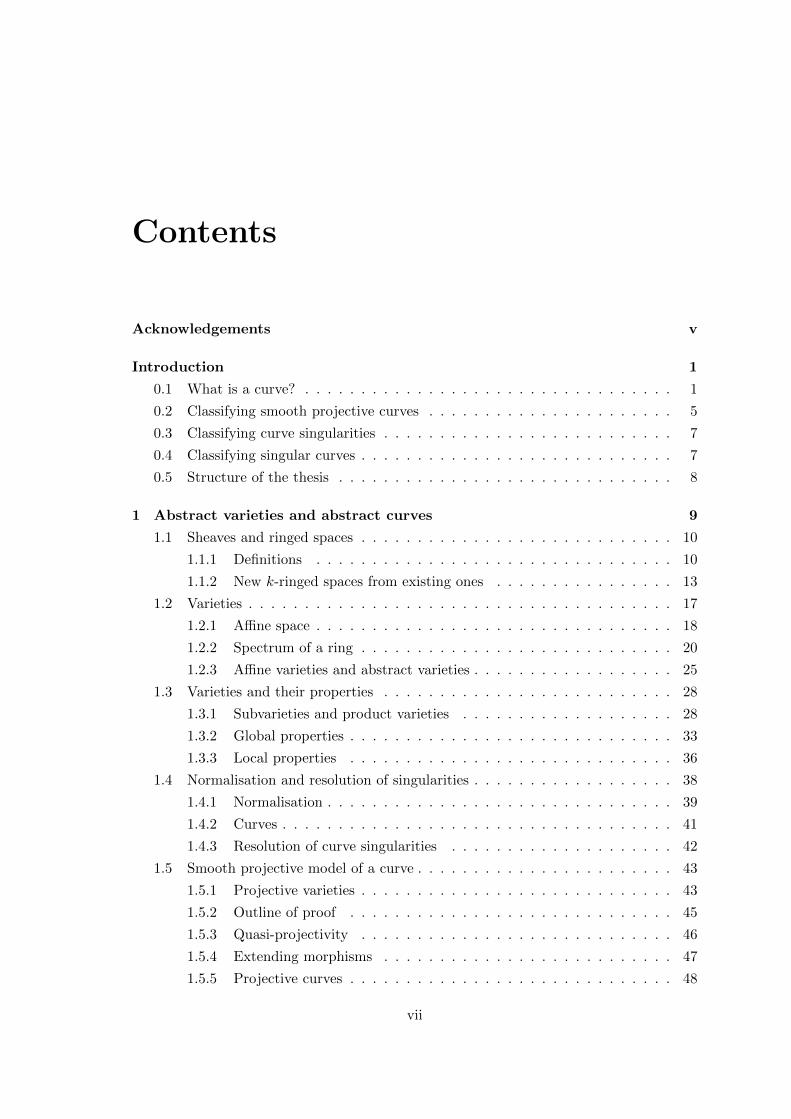
plane curves. The cusps and self-intersections in Figures 1b and 1c are referred to as

singular points, or singularities. Algebraically, singular points can be defined as follows:

1

2 CONTENTS

(a) C = V (y − x2). (b) V (y2 − x3) or the cuspidal cubic.

(c) V (y2 − x2 − x3) or the nodal cubic.

(d) V (x4 + x3 + x2y2 + 2x2y + 2xy +

y5 − 4y4 + 3y3).

Figure 1: Examples of algebraic curves and their real pictures.

Definition 0.1.2. A plane curve C = V (f) is singular at a point p ∈ C if ∂f/∂x(p) =

∂f/∂y(p) = 0. Otherwise, C is smooth at p. We say that C is smooth if it is smooth at

all points p ∈ C.

It is an immediate consequence of the implicit function theorem that any smooth curve

is a one-dimensional complex manifold, called a Riemann surface1. This identification is

extremely useful in the study of curves because it allows the application of a wide range

of tools from complex analysis.

Unfortunately, this approach is not directly applicable to singular curves because sin-

gular points prevent a curve from being a manifold. However, a classical theorem, first

proved by Riemann in 1851, shows that any singular curve can be approximated in a

unique way by a smooth curve, and hence by a Riemann surface [Kol07].

Theorem 0.1.3. Every curve is the projection of a unique smooth curve lying over it.

A precise formulation of this theorem is given in Theorem 1.4.11. Intuitively, this

theorem allows us to think of any curve, potentially singular, as the shadow of a smooth

1The terminology can be confusing, since a Riemann surface is a one-dimensional object. The term

surface is used because a Riemann surface has two real dimensions.

0.1. WHAT IS A CURVE? 3

x

y

z

(a) The cuspidal cubic (red) and its res-

olution of singularities (blue).

z

x

y

(b) View from above of the cuspidal cu-

bic and its resolution of singularities.

Figure 2: Resolution of singularities of the cuspidal cubic.

curve lying over it. The smooth projective curve associated to any given curve is called

its smooth projective model.

Since Riemann’s time, the resolution of singularities theorem for curves has been proven

in many different ways. One which appeals for its geometric nature is the method of “blow-

ups”, which we illustrate below with two examples [Hau03].

As a first example, consider the cuspidal cubic V (y2 − x3) with a singularity at the

origin, represented in Figure 1b. The method of blow-ups consists intuitively of lifting the

strands of the curve vertically into three-space, in order to obtain a smooth curve that

can be projected down onto the initial curve (see Figure 2).

A mathematical construction of this smooth curve from the cuspidal cubic is given by

considering the graph of the function (x, y) 7→ y/x, i.e. the set of points in 3-space of the

form (x, y, y/x). If we consider the cuspidal cubic as the image of the parametrisation

t 7→ (t2, t3), then post-composing this parametrisation with the above function yields a

curve parametrised by t 7→ (t2, t3, t). The derivative of this map is nowhere zero and so

the curve is indeed smooth. Moreover, as desired, it projects vertically down onto the

cuspidal cubic as seen in Figure 2b.

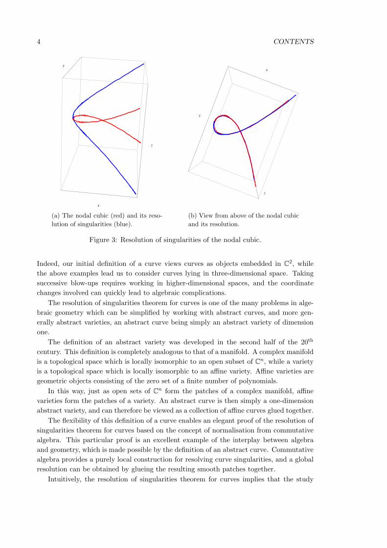
In the second example a similar approach provides a resolution of singularities of the

nodal cubic V (y2 − x2 − x3), pictured in Figure 1c. The nodal cubic is parametrised by

t 7→ (t2 − 1, t(t2 − 1)), so composing this parametrisation with the function (x, y) 7→ y/x

yields a curve parametrised by t 7→ (t2 − 1, t3 − t, t), which is again smooth. As seen in

Figure 3b, it projects down onto the nodal cubic.

While the method of blow-ups has the advantage of allowing visualisation of the process

of resolving the singularities of a curve, its proof requires revising the definition of a curve.

4 CONTENTS

x

y

z

(a) The nodal cubic (red) and its reso-

lution of singularities (blue).

z

x

y

(b) View from above of the nodal cubic

and its resolution.

Figure 3: Resolution of singularities of the nodal cubic.

Indeed, our initial definition of a curve views curves as objects embedded in C2, while

the above examples lead us to consider curves lying in three-dimensional space. Taking

successive blow-ups requires working in higher-dimensional spaces, and the coordinate

changes involved can quickly lead to algebraic complications.

The resolution of singularities theorem for curves is one of the many problems in alge-

braic geometry which can be simplified by working with abstract curves, and more gen-

erally abstract varieties, an abstract curve being simply an abstract variety of dimension

one.

The definition of an abstract variety was developed in the second half of the 20th

century. This definition is completely analogous to that of a manifold. A complex manifold

is a topological space which is locally isomorphic to an open subset of Cn, while a variety

is a topological space which is locally isomorphic to an affine variety. Affine varieties are

geometric objects consisting of the zero set of a finite number of polynomials.

In this way, just as open sets of Cn form the patches of a complex manifold, affine

varieties form the patches of a variety. An abstract curve is then simply a one-dimension

abstract variety, and can therefore be viewed as a collection of affine curves glued together.

The flexibility of this definition of a curve enables an elegant proof of the resolution of

singularities theorem for curves based on the concept of normalisation from commutative

algebra. This particular proof is an excellent example of the interplay between algebra

and geometry, which is made possible by the definition of an abstract curve. Commutative

algebra provides a purely local construction for resolving curve singularities, and a global

resolution can be obtained by glueing the resulting smooth patches together.

Intuitively, the resolution of singularities theorem for curves implies that the study

0.2. CLASSIFYING SMOOTH PROJECTIVE CURVES 5

of curves can be reduced to the study of smooth curves and how curve singularities are

attached to smooth curves.

As mentioned earlier, smooth curves are Riemann surfaces by the implicit function

theorem. By adding in so-called “points at infinity”, any curve can be made compact. The

resulting curves are called projective curves, which can be viewed as compact Riemann

surfaces. Conversely, any compact Riemann surface is a smooth projective curve. This is

a non-trivial result, but one which we accept as a given in this thesis. It can be proven

using the Riemann-Roch theorem, which implies the existence of non-zero meromorphic

functions on a compact Riemann surface [Mir95]. Thus the study of smooth projective

curves is equivalent to the study of compact Riemann surfaces.

0.2 Classifying smooth projective curves

Given a collection of objects and a notion of isomorphism between these objects, the

problem of their classification naturally arises. This problem is often tackled in two steps.

First, by trying to isolate discrete invariants which yield an initial, coarse classification of

the objects. Then, by trying to describe all objects with a given invariant. A priori this is

just a set. However, this set can often be parametrised by the points of a space, called a

moduli space. The word modulus is used in this context to suggest an idea of a continuous

variation of objects with a given invariant.

A paradigmatic example of this classification process is the case of compact Riemann

surfaces up to isomorphism, or equivalently of smooth projective curves up to isomorphism.

The problem of understanding the topology of compact Riemann surfaces was first

considered by Riemann in the 1850s. Based on Euler’s work on the characteristic of a

surface in the 1750s, Riemann defined the genus of a compact Riemann surface which is

essentially its number of holes. Figure 4 shows compact Riemann surfaces of genus 0, 1

and 2 respectively. Since two oriented surfaces are homeomorphic if and only if they have

the same genus, it follows that the genus of a compact Riemann surface is a complete

topological invariant.

The problem of classifying compact Riemann surfaces is therefore reduced to the prob-

lem of classifying compact Riemann surface with a given genus g up to isomorphism. In

other words, we wish to study the set:

Mg =

Compact Riemann surfaces of genus g

up to isomorphism

.

In the case of genus 0 compact Riemann surfaces, the problem is trivial. The Riemann

sphere, or equivalently P1, is up to isomorphism the only compact Riemann surface of

genus 0. Thus M0 = ∗.This is not the case for genus 1 surfaces. A genus 1 surface is a complex torus, and

hence can be represented by a lattice in the plane. Two such lattices determine isomorphic

tori if one can be obtained from the other by scaling, and the space of lattices up to scaling

can be shown to be in bijection with the complex numbers, using the j-elliptic function.

Thus M1 = C [BZ08].

6 CONTENTS

(a) Genus 0 Riemann surface. (b) Genus 1 Riemann surface. (c) Genus 2 Riemann surface.

Figure 4: Examples of Riemann surfaces.

The behaviour in the case of genus 1 suggests thatMg has more structure than a set.

This is also the case for higher genera. In fact, Mumford proved in 1965 that the set Mg

can be viewed as a 3g − 3 dimensional quasi-projective variety. In 1969, Mumford and

Deligne refined this result by showing that Mg is an irreducible variety [MFK02].

With this understanding of smooth projective curves the generalisation to arbitrary

smooth curves is relatively straightforward, because any smooth curve can be viewed as an

open subset of a smooth projective curve. This is a result which we will prove in Chapter

1 (Theorem 1.5.9). In this way, a smooth curve can be identified as a punctured compact

Riemann surface. Hence we define, analogously to Mg, the following set:

Mg,n =

Compact Riemann surfaces of genus g

with n punctures up to isomorphism

.

Isomorphisms of curves in Mg,n are required to fix the collection of punctures, though

they are allowed to permute the punctures. This space will play an important role in

Chapter 3 when classifying singular curves. The space Mg,n bears strong resemblance to

Mg. For example, the set Mg,n is also known to be a quasi-projective variety, similarly

to Mg [MFK02].

0.3 Classifying curve singularities

In the same way that there is a classification problem for smooth projective curves, there is

a classification problem for curve singularities. This problem was extensively studied in the

1960s by Zariski, who defined analytic and topological equivalence of curve singularities

[Zar06]:

Definition. Let X and Y be affine plane curves. Two singular points p ∈ X and q ∈ Yare analytically (resp. topologically) equivalent if there exist neighbourhoods U, V ⊆ C2

of p and q respectively and a biholomorphism (resp. homeomorphism) φ : U → V such

that φ(X ∩ U) = V ∩ Y .

0.4. CLASSIFYING SINGULAR CURVES 7

Both these concepts can be formulated purely algebraically; analytic equivalence can

be defined in terms of the complete local rings of curve singularities, while topological

equivalence can be defined in terms of the semigroups of these complete local rings. Intu-

itively, the semigroup of a curve singularity consists of the orders of vanishing of functions

in its corresponding complete local ring.

The fact that topological equivalence can be defined in terms of the semigroup of a

curve singularity is the result of an important theorem proved by Zariski in 1932 [Zar32].

This result states that two curve singularities are topologically equivalent if and only if

they have the same semigroup. Thus the semigroup of a curve singularity is a complete

topological invariant for curve singularities, just as the genus of a compact Riemann surface

is a complete topological invariant for compact Riemann surfaces.

Determining which semigroups arise as the semigroups of a curve singularity is rela-

tively straightforward and so the classification of curve singularities up to analytic equiv-

alence is reduced to the classification of curve singularities with a given semigroup up

to analytic equivalence. Applying the same idea used for compact Riemann surfaces, we

define:

MΓ =

Curve singularities with semigroup Γ

up to analytic equivalence

.

Zariski’s results regardingMΓ are compiled in his book Le probleme des modules pour

les branches planes. A large portion of this book is concerned with devising methods

for explicitly describing MΓ in a number of special cases. Zariski endows MΓ with a

topological structure, and shows that in generalMΓ is not quasi-projective. Nevertheless,

in those cases when MΓ is quasi-projective, Zariski poses the question of determining its

dimension, and whether it is irreducible. In contrast toMg, these problems remain open.

0.4 Classifying singular curves

The classification of singular curves starts with the search for discrete invariants. In fact,

we have already encountered them. Using the resolution of singularities theorem for curves

we can associate to any singular curve X, which we assume for simplicity has just one

singular point, a unique smooth curve X. As noted at the end of Section 0.2, this smooth

curve can naturally be identified with a punctured Riemann surface, and thus with a point

in Mg,n. We can also associate to X its singularity, which corresponds to a point in MΓ.

In this way, we can associate to a singular curve X three invariants: the genus g of X,

its number n of punctures, and the semigroup Γ of its singularity. These three invariants

define the topological type of a curve, which we write as a triple (g, n,Γ).

This is the first step in addressing the problem of classifying singular curves. As in

the case of compact Riemann surfaces and curve singularities, we define:

Mg,n,Γ =

Curves of topological type (g, n,Γ)

up to isomorphism

.

The set Mg,n,Γ admits a natural map Φ to the product Mg,n ×MΓ, which sends a

singular curve X to the pair consisting of its resolution of singularities X and its singular

8 CONTENTS

point.

To determine a singular curve in Mg,n, it suffices therefore to specify a smooth curve

Y in Mg,n, a singularity O in MΓ, and a point in the fibre Φ−1(Y,O). Intuitively the

choice of a point in the fibre consists of specifying how the singular point is glued on to

the smooth curve Y . We call this fibre the glueing space, and we will show in Chapter 3

that under suitable hypotheses, it is independent of the choice of smooth curve.

Thus a singular curve is completely determined by specifying a punctured compact

Riemann surface, a curve singularity, and how this singularity is glued on to the surface.

0.5 Structure of the thesis

In Chapter 1 we define the category of abstract varieties in order to arrive at the definition

of an abstract curve. We then prove that any curve admits a resolution of singularities

(Theorem 1.4.11) and that any smooth curve can be identified as an open subset of a

unique smooth projective (Proposition 1.5.10). This implies that any curve has a unique

smooth projective model. The material presented in this chapter is standard, compiled

from a number of references. Our presentation is perhaps closest to the one in Andreas

Gathmann’s notes [Gat14], but other resources used are: [Mum74], [Har77], [Muk03] and

[GW10]. The material in this section is admittedly dry, but has been included to keep

this thesis as self-contained as possible.

In Chapter 2 we study the classification of curve singularities based on Zariski’s meth-

ods introduced in Le probleme des modules pour les branches planes [Zar06]. We also

draw on more recent papers by Hefez and Hernandez [HH07, HHRH12]. We set up the

problem of the classification of curve singularities by identifying MΓ as the quotient of a

finite-dimensional affine space. We then compute explicit examples of the space MΓ.

In Chapter 3 we consider the classification of singular curves. We define the topological

type of a singular curve, and consider the problem of classifying all singular curves of a

given topological type. In particular, we reduce this problem to the problem of describing

how curve singularities can be glued on to a smooth curve, and provide an explicit algebraic

description of this glueing space. We then give some examples in which we explicitly

classify curves of a given topological type. The content of this chapter is original work

based on ideas suggested by my supervisor, David Smyth.

Chapter 1

Abstract varieties and abstract

curves

The purpose of this chapter is two-fold. First, we define the category of abstract varieties,

which leads to the definition of a curve as an abstract variety of dimension one. Then,

we prove two fundamental theorems about curves. The first is that any curve admits

a unique resolution of singularities (Theorem 1.4.11). The second is that any smooth

curve can be represented in a unique way as an open subset of a smooth projective curve

(Proposition 1.5.10). Together these results serve to show that the notion of an abstract

curve is consistent, perhaps surprisingly, with our geometric intuition of what an algebraic

curve should be. This chapter is quite technical and detailed in order to provide the

necessary formalism for our study of curves in Chapters 2 and 3.

In Section 1.1 we introduce the machinery of ringed spaces. These are topological

spaces together with a ring of functions on each of their open sets. We collect several

essential facts about ringed spaces that will be needed when defining varieties; most im-

portantly that ringed spaces can be glued (Construction 1.1.19), and that subspaces and

products of ringed spaces are themselves ringed spaces (Constructions 1.1.13 and 1.1.16).

In Section 1.2 we define affine varieties and abstract varieties (Definition 1.2.20). Affine

varieties are ringed spaces built from algebraic sets; a variety is a ringed space that is

locally isomorphic to an affine variety. We prove in this section that the category of affine

varieties is equivalent to the category of finitely-generated k-algebras (Corollary 1.2.28).

In Section 1.3 we show that subvarieties and products of varieties are varieties (Corol-

lary 1.3.3 and Proposition 1.3.7). We also define the dimension of a variety in terms of its

function field (Definition 1.3.20). Finally, we define the local properties of smoothness and

normality, which are key concepts in the proof of the resolution of singularities theorem

for curves.

In Section 1.4 we prove this theorem based on the concept of normalisation from

commutative algebra. We define normal varieties and show that every variety has a unique

normalisation (Proposition 1.4.2). In the case of curves, which satisfy the property that

smoothness and normality are equivalent notions, the resolution of singularities theorem

follows immediately.

Finally, in Section 1.5 we prove that any smooth curve is isomorphic to an open subset

9

10 CHAPTER 1. ABSTRACT VARIETIES AND ABSTRACT CURVES

of a unique smooth projective curve (Theorem 1.5.9), which we call its smooth projective

model.

Throughout this chapter, we let k denote a fixed algebraically closed field of charac-

teristic zero, and we let An denote a vector space of dimension n over k. We will identify

An as an affine variety in Section 1.2.

1.1 Sheaves and ringed spaces

In this section we define the category of k-ringed spaces. We start by defining a sheaf of

k-valued functions on a topological space (Definition 1.1.1), as well as a sheaf on the base

of a topology (Definition 1.1.4). The concept of a sheaf on a base will be needed when

constructing affine varieties as k-ringed spaces in Section 1.2. We define a k-ringed space

as a topological space together with a sheaf of k-valued functions (Definition 1.1.6). Open,

closed and locally closed subsets of k-ringed spaces, as well as products of k-ringed spaces

are given the structure of k-ringed spaces in Constructions 1.1.13 and 1.1.16. Finally, we

show how k-ringed spaces can be glued together to form new k-ringed spaces.

1.1.1 Definitions

A variety is a topological space together with a ring of functions on any open set of that

space. The idea of assigning to an open set of a topological space a ring of functions is

made precise by the notion of a sheaf.

Definition 1.1.1. Let X be a topological space. A sheaf OX of k-valued functions on X

is the assignment to every open set U in X of a k-algebra OX(U) of functions from U to

k subject to the following conditions:

(i) constant functions are in OX(U), and OX(U) is closed under addition and multipli-

cation, i.e. OX(U) is a k-subalgebra of all k-valued functions on U . Moreover, if

f ∈ OX(U) is nowhere vanishing on U , then 1/f ∈ OX(U). Finally, if f ∈ OX(U),

then D(f) = x ∈ U | f(x) 6= 0 is open in X;

(ii) if f ∈ OX(U) and U ′ is an open subset of U , then f |U ′ ∈ OX(U ′);

(iii) glueing axiom: let Uii be an open cover of U and let fi ∈ OX(Ui) satisfy fi|Ui∩Uj =

fj |Ui∩Uj for all i and j. Then the unique function f : U → k, defined by f |Ui = fifor all i, is an element of OX(U).

A function f ∈ OX(U) is said to be a regular function on U .

From here on, we use the term sheaf to mean sheaf of k-valued functions.

Condition (i) implies that regular functions form a subring of the ring of all functions

on a given open subset U of X. Furthermore, requiring D(f) to be open implies that

regular functions are continuous with respect to the topology on k defined by taking the

closed sets to be unions of finitely many points; this is the Zariski topology which we

will introduce in Section 1.2.1. Condition (ii) says that restrictions of regular functions

must be regular. An equivalent formulation of condition (iii), the glueing axiom, is that a

1.1. SHEAVES AND RINGED SPACES 11

function f : U → k is regular on U if and only if its restriction to each Ui in an open cover

Uii of U is regular on Ui. That is, a function is regular if and only if it is locally regular.

The local nature of the definition of a sheaf is fundamental to the definition of a ringed

space because it allows the “glueing” of such spaces, as we will see in Construction 1.1.19.

Example 1.1.2. Given a topological space X, the assignment to an open set U ⊆ X of

the ring of continuous functions f : U → R defines a sheaf on X. This follows from the

fact that continuity is a local property.

Example 1.1.3. The assignment to every open set U ⊆ X of all constant functions

f : U → X is not necessarily a sheaf on X. To see this, suppose that X is disconnected,

say X = X1tX2. If we consider the case in which two constant functions f1 and f2 on X1

and X2 respectively take on distinct values in k, then the function f defined by f |Xi = fiis not globally constant. Thus f1 and f2 do not glue to a constant function on X, despite

satisfying the compatibility conditions. Heuristically, the reason why this assignment is

not a sheaf on X is that being constant is a global property rather than a local property.

We can nevertheless obtain a sheaf on X by assigning to each open set in X the ring of

locally constant functions instead.

By definition, a sheaf on X is determined by the data consisting of a ring of functions

for any open subset U of X. However, given a base B for the topology on X, a sheaf on X

can be constructed from the data consisting of the assignment of a ring of functions solely

to open sets B ∈ B, rather than all open sets U ⊆ X. This will be a useful construction

when defining affine varieties in Section 1.2.

Definition 1.1.4 (Sheaf on a base). Let X be a topological space with base B. A sheaf

of k-valued functions on the base B is the assignment to every open set B ∈ B of a ring

OX(B) of functions from B to k such that:

(i) constant functions are in OX(B), and OX(B) is closed under addition and multipli-

cation, i.e. OX(B) is a k-subalgebra of all k-valued functions on B. Moreover, if

f ∈ OX(B) is nowhere vanishing on B, then 1/f ∈ OX(B). Finally, if f ∈ OX(B),

then D(f) = x ∈ B | f(x) 6= 0 is open;

(ii) if f ∈ OX(B) and B′ ∈ B is an open subset of B, then f |B′ ∈ OX(B′);

(iii) Let Bii be an open cover of B and let fi ∈ OX(Bi) satisfy fi|Bi∩Bj = fj |Bi∩Bj for

all i and j. Then the unique function f : B → k defined by f |Bi = fi for all i is an

element of OX(B).

Proposition 1.1.5. Let X be a topological space with base B. If OX is a sheaf on the

base B of X, then this sheaf can be extended to a sheaf on X by declaring:

OX(U) = f : U → k | f |B ∈ OX(B) for any B ∈ B

for any open subset U ⊆ X.

Proof. All three axioms from Definition 1.1.1 follow immediately from the definition of

OX(U) and by virtue of OX being a sheaf on the base B.


We can now define a k-ringed space simply as a topological space together with a sheaf.

Definition 1.1.6. A k-ringed space (X,OX) is a topological space X together with a

sheaf OX on X. The ring OX(X) consists of functions which are regular on all of X.

These are called global regular functions on (X,OX).

Notation 1.1.7. For ease of notation, we often identify a k-ringed space (X,OX) with

its underlying topological space X.

Example 1.1.8. If X is a complex manifold, we can obtain a C-ringed space by consid-

ering the sheaf which associates to an open set U ⊆ X the ring of holomorphic functions

on U .

Note that we can define a k-ringed space for fields that are not algebraically closed.

If X is a smooth real manifold, we can obtain an R-ringed space by considering the sheaf

which associates to an open set U ⊆ X the ring of infinitely differentiable functions on U .

Definition 1.1.9. Let (X,OX) and (Y,OY ) be k-ringed spaces. A morphism from

(X,OX) to (Y,OY ) is a continuous function f : X → Y such that, for any open set

U in Y , the following holds:

g ∈ OY (U)⇒ g f ∈ OX(f−1(U)).

Given an element g ∈ OX(U), we call the composition g f the pull-back of g by f .

The map f is an isomorphism if it admits an inverse morphism.

In other words, a morphism is a continuous function which pulls back regular functions

to regular functions.

Notation 1.1.10. By definition, a morphism f : X → Y induces a homomorphism

OY (U)→ OX(f−1(U)) for any open set U in Y . We denote this induced map by f∗.

Remark 1.1.11. It follows from the definition that the composition of morphisms is a

morphism. Moreover, the identity map from a k-ringed space to itself is a morphism.

With this notion of a morphism between k-ringed spaces, we can consider the set of

k-ringed spaces as a category.

Example 1.1.12. Holomorphic maps of complex manifolds are morphisms of k-ringed

spaces. To see this, let X and Y be n and m-dimensional complex manifolds respectively,

and let f be a map from X to Y . Given x ∈ X, there exists a neighbourhood U of x

that is isomorphic to an open set of Cn via a chart φ. Similarly, there is a neighbourhood

V of f(x) ∈ Y that is isomorphic to an open set of Cm via a chart ψ. The map f is a

holomorphic map if the composition ψ f φ−1 is holomorphic at φ(x).

If g is a function that is holomorphic at f(x) ∈ Y , then by definition g ψ−1 is

holomorphic at ψ(f(x)) ∈ Cm. The composition g f is holomorphic at x ∈ X, since

g f φ−1 = g ψ−1 ψ f φ−1 which is holomorphic at φ(x).

Building on Example 1.1.8, we can therefore view the category of complex manifolds

as a full subcategory of the category of k-ringed spaces:category of

complex manifolds

⊆

category of

k-ringed spaces

.


Thus the category of k-ringed spaces can be understood as an enlargement of the

category of manifolds, by considering a larger class of topological spaces and functions.

This is one way of making sense of the definition of a k-ringed space.

1.1.2 New k-ringed spaces from existing ones

There are many useful ways to obtain new k-ringed spaces from existing ones. We describe

three ways to do so: by taking subspaces of a given k-ringed space, by taking the product

of two k-ringed spaces, and by glueing together a collection of k-ringed spaces.

Construction 1.1.13 (Open, closed and locally closed k-ringed subspaces).

(i) If U is an open subset of the underlying topological space of a k-ringed space (X,OX),

then U has an induced k-ringed space structure. Indeed, the open set U with the

subspace topology naturally inherits a sheaf, denoted OX |U , via the restriction of

functions on X to U . The pair (U,OX|U ) is then a k-ringed space. We say that

(U,OX|U ) is an open k-ringed subspace of (X,OX).

(ii) If Y is a closed subset of X, then the situation is more complicated. Open subsets of

Y are not necessarily open subsets of X, and so we cannot just take the restriction

of the sheaf on X. Instead, we define a sheaf on U by declaring for any open subset

U of Y :

OY (U) :=

f : U → k

∣∣∣∣∣∣∣∣∣∣for any y ∈ U , there exists

an open neighbourhood V ⊆ X of y

and a function g ∈ OX(V ) such that

g|U∩V = f

.

It is clear that this assignment defines a sheaf on Y , because of the local nature of

its definition. We call (Y,OY ) a closed k-ringed subspace of X.

(iii) If Z is a locally closed subspace of X, that is, the intersection of an open subset U

and a closed subset Y of X, then Z has an induced k-ringed space structure either

by considering Z as an open subset of the k-ringed space Y , or by considering Z as a

closed subset of U . In fact, both perspectives yield the same k-ringed space structure

on Z and we call (Z,OZ) a locally closed k-ringed subspace of X. Note that open and

closed k-ringed subspaces can both be viewed as locally closed k-ringed subspaces.

For this reason, we define a k-ringed subspace to be a locally closed k-ringed subspace.

Remark 1.1.14. It follows from the definition of an open k-ringed subspace that the

restriction of a morphism to an open subset is again a morphism. Moreover, if (Y,OY )

is a k-ringed subspace of (X,OX), then the inclusion i : Y → X is a morphism of k-

ringed spaces. Indeed, if g ∈ OX(U) for some U open in X, then g i is a function on

i−1(U) = Y ∩ U . But g i = g|Y ∩U , and so by definition of the sheaf on Y , we have that

g i = OY (i−1(U)).

With this understanding of k-ringed subspaces, we can now prove a useful property of

morphisms between k-ringed spaces which will be needed in the proof of Proposition 1.2.25.


Proposition 1.1.15. Suppose that (X,OX) and (Y,OY ) are k-ringed spaces and let

(Z,OZ) be a k-ringed subspace of (Y,OY ). Let i denote the inclusion of Z into Y . Suppose

that f : X → Y is a map satisfying f(X) ⊆ Z, so that we have the following commutative

diagram:

Xf //

f

Y

Z.i

>>

Then f is a morphism of k-ringed spaces if and only if f is a morphism of k-ringed

spaces.

This property is a convenient way of obtaining morphisms from a k-ringed space X to

an open or locally closed subset Z of another k-ringed space Y . Indeed, by this proposition,

in order to give a morphism from X to Z it suffices to give a morphism from X to Y that

has image lying in Z.

Proof. It is clear that if f is a morphism, then so is f by composing the morphism f with

the inclusion morphism.

Conversely, suppose that f is a morphism. The map f is continuous by the definition

of the induced topology on Z. We start by proving the proposition in the case when Z is

open. The fact that regular functions pull back to regular functions is immediate from the

observation that OZ(U) = OY (U) for open set U in Z, by definition of the sheaf induced

on Z.

Next, suppose that Z is closed, and let g ∈ OZ(U). By definition of the sheaf induced

on Z, the function g is locally of the form i∗g′ for some g′ ∈ OY (V ). Hence locally on

f−1

(U) we have:

f∗g = f

∗(i∗g′) = f∗g′.

It follows that f∗(g) is regular on f

−1(U).

The statement for a locally closed subset follows immediately, since a locally closed

subset can be viewed as an open subset inside a closed k-subringed space (or as a closed

subset inside an open k-subringed space).

We now show how to construct the product of two k-ringed spaces X and Y as a

k-ringed space.

Construction 1.1.16 (Product of k-ringed spaces). The set X × Y is simply the set-

theoretic product of X and Y . Its topology however is not the product topology. Let

gini=1 be a collection of regular functions on an open subset U of X, and hini=1 a

collection of regular functions on an open subset V of Y . Define a function f on U × Vby f(u, v) =

∑ni=1 gi(u)hi(v).

We define the topology on X × Y by declaring a base B for the topology to be the

collection of sets Bf of the form Bf = (u, v) ∈ U × V | f(u, v) 6= 0 where U, V are

open in X and Y respectively, and f is as above. Note that this topology is finer than the

product topology.


We then define a sheaf on the base B of the topology on X × Y by assigning to any

open set Bf as above the ring of functions:

OX×Y (Bf ) :=

f ′

f

∣∣∣∣ f ′(u, v) =n∑i=1

g′i(u)h′i(v) where g′i ∈ OX(U) and h′i ∈ OY (V )

.

Definition 1.1.17. The product X × Y constructed above is called the k-ringed space

product of X and Y .

Remark 1.1.18. It follows from its construction that the above product satisfies the

universal property in the category of k-ringed spaces [Kem93, Lemma 3.1.1.].

The most useful construction of k-ringed spaces from existing k-ringed spaces however

is via a method called glueing. Such a construction is possible because of the local definition

of a sheaf of k-valued functions which allows compatible functions on an open cover to be

glued together to form a function on the covered open set.

Construction 1.1.19 (Glueing k-ringed spaces). Let (Xi,OXi)i∈I be a collection of k-

ringed spaces. Suppose that we have for every i, j an open subset Uij ⊆ Xi and a k-ringed

space isomorphism:

ϕij :(Uij ,OXi|Uij

)→(Uji,OXj |Uji

)satisfying:

(i) ϕii = id(Xi,OXi ),

(ii) ϕ−1ij = ϕji, and

(iii) ϕik = ϕjk ϕij (cocycle condition).

We construct a k-ringed space (X,OX) together with maps ιi : Xi → X such that:

(i) Each ιi maps Xi isomorphically onto its image,

(ii) ι−1i (ιj(Xj)) = Uij ⊆ Xj ,

(iii) ι−1j ιi : Uij → Uji is ϕij .

The construction of X will be done in three steps. We start by defining X as a set

(see 1) below), then as a topological space (see 2) below), and finally as a k-ringed space

(see 3) below). We then prove that the ringed spaces (Xi,OXi) are isomorphic to open

k-ringed subspaces of (X,OX), and that above three conditions are satisfied.

1) As a set: Let

X :=⊔i

Xi/ ∼

where ∼ is the equivalence relation defined by x ∼ ϕij(x) for any x ∈ Uij . The fact

that this is an equivalence relation follows from the properties of the maps ϕij . Indeed,

since ϕii(x) = id, we have that x ∼ x. Since ϕij = ϕ−1ji , the relation is symmetric. The

cocycle condition ensures transitivity of the relation.


2) As a topological space: Let ιi : Xi → X denote the natural inclusion of Xi into X. We

define a topology on X by declaring W ⊆ X to be open if and only if ι−1i is open in

Xi for all i. With this topology, the maps ιi are homeomorphisms onto their images in

X. Note that by construction of X, ιi = ιj ϕij on Uij .

3) As a k-ringed space: To endow X with the structure of a k-ringed space, we need to

construct a sheaf OX on X. Let W ⊆ X be open. We define OX(W ) by

OX(W ) := f : W → k | f ιi ∈ OXi(ι−1i (W )).

We now show that OX defined in this way is a sheaf on X, by verifying that the three

conditions from Definition 1.1.1 are satisfied. The fact that OXi are sheaves on Xi

implies immediately that conditions (i) and (ii) are satisfied. To show condition (iii),

suppose that Vαα is an open cover of W , and that for each α there exists some

fα ∈ OX(Vα) such that fα|Vα∩Vβ = fβ|Vα∩Vβ . Our aim is to show that the function

f : W → k defined by f |Vα = fα is in OX(W ).

The collection ι−1i (Vα)α is a cover of ι−1

i (W ). Moreover, we have that fα ιi ∈OXi(ι

−1i (Vα)) for all i and that

fα ιi|ι−1i (Vα∩Vβ) = fβ ιi|ι−1

i (Vα∩Vβ).

By virtue of OXi satisfying the glueing axiom, the function gi defined by gi|ι−1i (Vα) =

fα ιi is an element of OXi(ι−1i (W )). Since this holds true for each i, we have a

collection gii such that each gi ∈ OXi(ι−1i (W )).

Furthermore, these functions gi are compatible when viewed as functions on W , by

pre-composing with ι−1i . Indeed, if we consider the open cover of ιi(Uij) given by

ιi(Uij) ∩ Vαα, then

gi ι−1i |ιi(Uij)∩Vα = fα|Vα∩ιj(Uji) = fα|Vα∩ιi(Uij) = gj ι−1

j |ιj(Uji)∩V (α).

Since this holds true for every α, it follows that the functions gi satisfy

gi ι−1i |ιi(Uij) = gj ι−1

j |ιj(Uji). (1.1)

Since ιi(Uij) = ιj(Uji), this condition exactly implies that the map g : W → k defined

by

g|W∩ιi(Xi) = gi ι−1i |W∩ιi(Xi)

is a well-defined function on W . Indeed, if x ∈W ∩ ιi(Xi) ∩ ιj(Xj), then gi ι−1i (x) =

gj ι−1j (x) by (1.1).

By construction of g, it is clear that g ∈ OX(W ). Since g and f agree on the open

cover Vαα of W , they are equal on W which implies that f ∈ OX(W ). Thus OX is

a sheaf on X, and so (X,OX) is a k-ringed space.

1.2. VARIETIES 17

4) It remains only to show that the map ιi : (Xi,OXi)→(ιi(Xi),OX|ιi(Xi)

)is an isomor-

phism of k-ringed spaces.

Let U ⊆ Xi be an open subset. By the definition of a k-ringed space isomorphism,

it suffices to show that g ∈ OX|ιi(Xi)(ιi(U)) if and only if g ιi ∈ OXi(U). One

direction is immediate: if g ∈ OX|ιi(Xi)(ιi(U)) then by definition of OX , we have that

g ιi ∈ OXi(U).

To show the converse, suppose that g ιi ∈ OXi(U). Then since ϕji is an isomorphism

of k-ringed spaces, we have that

g ιi ϕji = g ιj ∈ OXj (ϕij(U)) = OXj (ι−1j (ιi(U))).

So by definition, g ∈ OX|ιi(Xi)(ιi(U)).

Thus (Xi,OXi) ∼=(ιi(Xi),OX|ιi(Xi)

)as k-ringed spaces, and it is clear that the maps

ιi satisfy the properties (i), (ii) and (iii).

Morphisms of k-ringed spaces also satisfy a glueing property.

Proposition 1.1.20 (Glueing morphisms). Let X and Y be k-ringed spaces, and let Uiibe an open cover of X by k-ringed spaces. Let fi : Ui → Y i be a collection of morphisms

of k-ringed spaces satisfying fi|Ui∩Uj = fj |Ui∩Uj for all i, j. Then the map f : X → Y

defined by f |Ui = fi is a morphism of k-ringed spaces.

Proof. It is clear that f is a continuous map since continuity is a local property. Now let

W ⊆ Y be an open subset and suppose that g ∈ OY (W ). We wish to show that g f ∈OX(f−1(W )). We know that (g f)|f−1(W )∩Ui = g (f |f−1(W )∩Ui) ∈ OX(f−1(W ) ∩ Ui)because f |f−1(W )∩Ui is a morphism by Remark 1.1.11.

Since f−1(W )∩Uii is an open cover of f−1(V ), then by the glueing axiom of sheaves

the map g f : f−1(V )→ Y is in OX(f−1(W )).

These glueing constructions are fundamental to the definition of a variety.

1.2 Varieties

In this section we define affine varieties and abstract varieties. An affine variety is a k-

ringed space where the topological space is an irreducible algebraic set of An endowed with

the Zariski topology, and where the regular functions are locally quotients of polynomials.

A variety is a k-ringed space which admits a cover by affine varieties.

In Section 1.2.1 we give An the structure of an affine variety, to provide intuition for

the definition of an affine variety. In Section 1.2.2 we adopt a more abstract approach and

see how a k-ringed space can be recovered from an arbitrary finitely generated integral

k-algebra. The k-ringed spaces constructed in this way are affine varieties. In Section

1.2.3 we prove an equivalence of categories between affine varieties and finitely generated

integral k-algebras.


1.2.1 Affine space

To endow An with a k-ringed space structure, we start by constructing a topology on An.

Definition 1.2.1. Given an ideal a in k[x1, . . . , xn], we define the set

V (a) := x ∈ An | f(x) = 0 for all f ∈ a.

Given the ideal (f1, . . . , fk) generated by f1, . . . , fk ∈ k[x1, . . . , xn], we write V (f1, . . . , fk)

instead of V ((f1, . . . , fk)) to simplify notation. Such sets are called algebraic subsets of

An.

Remark 1.2.2. By Hilbert’s basis theorem, the ring k[x1, . . . , xn] is noetherian. Hence

any ideal a ⊆ k[x1, . . . , xn] is finitely generated, so that V (a) = V (f1, . . . , fk) for some

f1, . . . , fk ∈ k[x1, . . . , xn]. In this way, algebraic subsets of An consist of the vanishing

locus of a finite number of polynomials in k[x1, . . . , xn].

We can define a topology on An by declaring the algebraic subsets to be its closed

subsets. The fact that this defines a topology on An follows from the following three

properties of algebraic subsets:

(1) If aii is an arbitrary family of ideals in k[x1, . . . , xn], then

⋂i∈I

V (ai) = V

(∑i∈I

ai

).

(2) If a and a′ are two of ideals of k[x1, . . . , xn], then

V (a) ∪ V (a′) = V(aa′).

(3) V (k[x1, . . . , xn]) = ∅ and V (0) = An.

Definition 1.2.3. The topology on An defined by taking sets of the form V (a) to be the

closed subsets is called the Zariski topology. Given f ∈ k[x1, . . . , xn], we let D(f) denote

the open set An \ V (f). Such sets are called distinguished open sets.

Distinguished open subsets of An form a base for the topology. This follows from the

fact that D(f) ∩ D(g) = D(fg) and that any open set An \ V (a) can be written in the

form

An \ V (a) =⋃f∈a

D(f).

We now construct a sheaf on the topological space An. By Proposition 1.1.5, it suffices

to construct a sheaf on the base of An given by the distinguished open subsets D(f). We

define:

OAn(D(f)) := k[x1, . . . , xn]f =

a

fm| a ∈ k[x1, . . . , xn] and m ∈ N

.

1.2. VARIETIES 19

Elements ofOAn(D(f)) can naturally be viewed as functions on An: an element a/fm ∈OAn(D(f)) sends x ∈ An to a(x)/f(x)m, which is a well-defined map since f(x) 6= 0 for

all x ∈ D(f).

By Proposition 1.1.5, we obtain a sheaf on An by defining:

OAn(U) := g : U → k | g|D(f) ∈ OX(D(f)) for any D(f) ⊆ U.

Equivalently, we can write:

OAn(U) =⋂

D(f)⊆U

OAn(D(f)).

The ring of global regular functions of An is then given by:

OAn(An) =⋂

D(f)⊆AnOAn(D(f)) =

⋂f∈k[x1,...,xn]

k[x1, . . . , xn]f

= k[x1, . . . , xn],

which we call the coordinate ring of An.

In this way, we can think of the k-ringed space (An,OAn) as the triple consisting of

its underlying set An, its Zariski topology and its sheaf OAn . We will now explain how

these three objects can be recovered from a single algebraic object: the coordinate ring

k[x1, . . . , xn] of An.

The starting point is the following important result from algebraic geometry, which

relates the maximal ideals of k[x1, . . . , xn] to the points of An. Its proof is given in the

appendix, see Proposition A.1.5.

Proposition A.1.5 (Weak Nullstellensatz). The maximal ideals in k[x1, . . . , xn] are the

ideals of the form (x1 − a1, . . . , xn − an) for some (a1, . . . , an) ∈ An.

Notation 1.2.4. We let xm denote the point in An corresponding to the maximal ideal

m in k[x1, . . . , xn]. Conversely, we let mx denote the maximal ideal in k[x1, . . . , xn] corre-

sponding to the point x in An.

In this way, points in An can be identified with maximal ideals in k[x1, . . . , xn], and so

the underlying set of An is, as desired, determined by the coordinate ring k[x1, . . . , xn].

Recall from Definition 1.2.3 that the topology on An was given by defining sets of the

form V (a) to be closed. By definition, we have the following sequence of equivalences:

x ∈ V (a)⇔ f(x) = 0 for all f ∈ a

⇔ f ∈ mx for all f ∈ a⇔ a ⊆ mx. (1.2)

Hence we can view V (a) as the set of all maximal ideals of k[x1, . . . , xn] containing a.

Thus the topology on An is also determined by the ring of global k[x1, . . . , xn].

We have already defined the sheaf on An in terms of localisations of k[x1, . . . , xn], and

so it follows that the k-ringed space An is indeed determined only by the coordinate ring

k[x1, . . . , xn].


1.2.2 Spectrum of a ring

In this section we will construct k-ringed spaces that are determined not just by polynomial

rings but by finitely generated integral k-algebras, that is, rings of the form k[x1, . . . , xn]/p

for some prime ideal p ⊆ k[x1, . . . , xn]. Given a finitely-generated integral k-algebra A, we

denote the corresponding k-ringed space by (SpecA,OSpecA). Such spaces will be called

affine varieties.

The construction will be done in three steps: we start by defining SpecA as a set

(Definition 1.2.5), then as a topological space (Definition 1.2.8), and finally as a k-ringed

space (Definition 1.2.18).

Since A is a finitely generated integral k-algebra, we have that A ∼= k[x1, . . . , xn]/p

for some prime ideal p ⊆ k[x1, . . . , xn]. From here on, we fix the isomorphism from A to

k[x1, . . . , xn]/p, and identify both objects.

1) As a set:

Definition 1.2.5. The spectrum of A, denoted SpecA, is the set

SpecA := m ⊂ A | m is a maximal ideal.

If a is an ideal of A, we define V (a) to be the set of all maximal ideals of A containing

a. As in Definition 1.2.1, we write V (f) for V ((f)) where (f) is the ideal generated by

f ∈ A.

Remark 1.2.6.

(i) The overlap of notation with that used in Definition 1.2.1 is deliberate, as both

definitions agree under the identification of maximal ideals in k[x1, . . . , xn] with

points in An described in Notation 1.2.4. Indeed, as derived in (1.2),

V (a) = x ∈ An | f(x) = 0 for all f ∈ a = m ∈ SpecA | a ⊆ m = V (a),

where the V (a) on the left is taken in the sense of Definition 1.2.1, and the V (a)

on the right is taken in the sense of Definition 1.2.5.

(ii) The set SpecA is the set of all maximal ideals of A, which is the set of all

maximal ideals of k[x1, . . . , xn]/p. But these ideals are exactly the maximal ideals

of k[x1, . . . , xn] containing p, which corresponds to the set V (p). We can therefore

identify the set SpecA with the vanishing locus V (p) ⊆ An of the ideal p. This

identification will be useful in our construction of SpecA as a k-ringed space in

4).

2) As a topological space: We define a topology on SpecA by declaring sets of the form

V (a) to be closed. The following proposition shows that this does indeed define a

topology on SpecA:

1.2. VARIETIES 21

Proposition 1.2.7.

(i) V (0) = SpecA and V (1) = ∅;(ii) If aii is an arbitrary collection of ideals of A, then

⋂i∈I

V (ai) = V

(⋃i∈I

ai

);

(iii) If a, a′ are two ideals of A, then

V (a) ∪ V (a′) = V (aa′).

Proof. Assertion (i) follows from the observation that every maximal ideal contains the

ideal (0), and that there are no maximal ideals containing (1) (since maximal ideals

must be proper).

Assertion (ii) follows from the observation that m ∈⋂i∈I V (ai) if and only ai ⊆ m for

all i ∈ I, which is equivalent to having that m ∈ V(⋃

i∈I V (ai)).

To show assertion (iii), we observe that the maximal ideal m contains a or a′ if and

only if m contains the product aa′. Note that this property holds true for all prime

ideals, not necessarily maximal.

Definition 1.2.8. The topology defined on SpecA by declaring sets of the form V (a)

to be the closed subsets is called the Zariski topology on SpecA. Note that for A =

Spec k[x1, . . . , xn], it is the same as the Zariski topology on An defined in Section 1.2.1,

under the identification described in Remark 1.2.6

The Zariski topology has three useful properties which will be needed to obtain a sheaf

of functions on SpecA in Proposition 1.2.19; it has a base of open sets of the form

SpecA\V (f) for some f ∈ A, it is quasi-compact, and it is noetherian.

Definition 1.2.9. Given f ∈ A, we let D(f) denote the open set

SpecA \ V (f) = m ⊆ A | f /∈ m.

Such sets are called distinguished open sets.

Remark 1.2.10. In the case where A = k[x1, . . . , xn], these distinguished open sets

are the same as those defined in Definition 1.2.3 under the identification described in

Notation 1.2.4.

Proposition 1.2.11. The set of all subsets of SpecA of the form D(f) for some f ∈ Aform a base for the Zariski topology on SpecA.

Proof. Let U ⊆ SpecA be open. Then U is of the form SpecA \ V (a) for some ideal

a ⊆ A. We have that

SpecA \ V (a) = m ⊆ A | a * m = m ⊆ A | f /∈ m for all f ∈ a =⋃f∈a

D(f).


Hence every open set in SpecA can be written as a union of distinguished open sets.

Moreover, the intersection of two distinguished open sets is itself a distinguished open

set:

D(f) ∩D(g) = D(fg).

Indeed, f or g is an element of a maximal ideal m if and only if fg is an element of m

by virtue of m being a prime ideal.

Thus the distinguished open sets D(f) form a base for the Zariski topology on SpecA.

The second important and useful property of the Zariski topology is that it is quasi-

compact.

Proposition 1.2.12. Suppose that SpecA =⋃i∈I D(fi). Then there exist elements

f1, . . . , fn ∈ fii∈I such that SpecA =⋃nj=1D(fj).

Proof. We have:

SpecA =⋃i∈I

D(fi) = D

(∑i∈I

(fi)

).

Taking complements, we have that V (∑

i∈I(fi)) = ∅. This implies that there are no

maximal ideals containing∑

i∈I(fi), from which we can conclude that A =∑

i∈I(fi).

Hence 1 ∈∑

i∈I(fi) and can be written as a finite sum∑n

j=1 fj where fj ∈ fii∈I for

all j. Thus we have that∑

i∈I(fi) =∑n

j=1(fj).

It follows that

SpecA = D

n∑j=1

(fj)

=

n⋃j=1

D(fj),

which shows that X is covered by only finitely many of the D(fi)s.

The third property satisfied by the Zariski topology is that it is noetherian.

Definition 1.2.13. A topological space X is noetherian if every descending chain

Z1 ⊃ Z2 ⊃ · · · of closed subsets of X terminates.

Proposition 1.2.14. SpecA is noetherian.

Proof. If V (a1) ⊃ V (a2) ⊃ · · · is an infinite descending chain of closed subsets in

SpecA, then we have a corresponding ascending chain of ideals√a1 ⊂

√a2 ⊂ · · ·

in A by Corollary A.1.9. Let a =⋃∞i=1

√ai. Then a is an ideal in A, and since A

is noetherian, it must be finitely generated. Thus the chain terminates after finitely

many terms only.

Remark 1.2.15. By contrast, the topological space R with the Euclidean topology

is not noetherian. For example the chain of closed subsets [−1, 1] ⊃ [−1/2, 1/2] ⊃[−1/4, 1/4] ⊃ · · · does not terminate.

1.2. VARIETIES 23

It follows from the fact that SpecA is noetherian that any subset can be expressed as

a finite union of irreducible subsets.

Definition 1.2.16. A topological space X is irreducible if given closed subsets X1 and

X2 of X,

X = X1 ∪X2 ⇒ X = X1 or X = X2.

Otherwise, we say that X is reducible.

Proposition 1.2.17. Any set X ⊆ SpecA can be decomposed as a finite union X1 ∪· · · ∪Xr of irreducible subsets of SpecA.

Proof. If X is irreducible, the statement trivially holds, so we assume that X is re-

ducible. Then X = X1∪X2 for some proper subsets X1, X2 ⊂ X. If one or both of the

sets Xi are reducible, then we can further decompose them. This process must stop

after a finite number of steps, since we would otherwise obtain an infinite descending

chain of closed subsets, contradicting the fact that SpecA is noetherian.

We can now endow the topological space SpecA with the structure of a k-ringed space.

3) As a k-ringed space:

We can think of an element f ∈ A as a function on SpecA by defining f(m) := f ∈ A/m,

where f is the image of f under the quotient map from A to A/m. Note that A/m ∼= k

by Proposition A.1.5 so f is indeed a k-valued function.

We can now construct a sheaf OSpecA of k-valued functions on the topological space

SpecA to obtain a k-ringed space (SpecA,OSpecA). Just as we did for An, we only

assign a ring of functions to distinguished open subsets D(f) of SpecA, which will yield

a sheaf on SpecA by Proposition 1.1.5.

Definition 1.2.18. Given a distinguished open subset D(f) ⊆ SpecA, we define

OSpecA(D(f)) := Af .

Proposition 1.2.19. OSpecA defines a sheaf of k-valued functions on the base of the

topology on SpecA consisting of the distinguished open sets.

Proof. We must show that the three conditions from Definition 1.1.4 hold.

(i) It is clear that OSpecA(D(f)) is a k-subalgebra of all k-valued functions on D(f).

Suppose that g = a/fn ∈ OSpecA(D(f)) vanishes nowhere. Then D(f) ⊆ D(g),

so we have by Corollary A.1.9 that

(f) ⊆√

(g).

Hence there exists an m ∈ N such that fm = a′g, where a′ ∈ A. In this way, we

can write 1/g = a′/fm, which is an element of Af and so 1/g ∈ OSpecA(D(f)).


(ii) Suppose that D(f) ⊆ D(g), and let a/gn be an element of Ag. Since D(f) ⊆ D(g),

we have that√f ⊆ √g. Hence fm = a′g for some a′ ∈ A, from which it follows

thata

gn=aa′n

fmn,

which is an element of Af . Thus the function a/gn, when restricted to D(f), is

an element of OSpecA(D(f)).

(iii) Finally, we show that if there exists a collection of open sets D(fi) which covers

D(f) and functions gi ∈ OSpecA(D(fi)) such that

gi|D(fi)∩D(fj)=D(fifj) = gj |D(fifj),

then the function g defined by g|D(fi) = gi is an element of OSpecA(D(f)).

By quasi-compactness we can easily reduce to the case where the cover of D(f)

is finite:

D(f) =

n⋃i=1

D(fi).

Each element gi ∈ OSpecA(D(fi)) can be written in the form ai/fkii for some

ai ∈ A and ki ∈ N. By the compatibility condition, we have:

ai

fkii

∣∣∣∣∣D(fifj)

=aj

fkjj

∣∣∣∣∣D(fifj)

.

Equivalently, we have:

aifkjj − ajf

kii = 0. (1.3)

Since

D(f) =

n⋃i=1

D(fi) =

n⋃i=1

D(fkii ),

it follows that:

V (f) =n⋂i=1

V (fkii ) = V(

(fk11 , . . . , fknn )).

Hence√

(f) =√

(fk11 , . . . , fknn ), and so there exists some m ∈ N and ri ∈ A such

that:

fm =

n∑i=1

rifkii .

We now define:

g =

∑ni=1 riaifm

∈ OSpecA(D(f)).

It remains only to check that g|D(fj) = aj/fkjj . But this follows from the fact

that:

gfkjj =

∑ni=1 riaif

kjj∑n

i=1 rifkii

=

∑Ni=1 riajf

kii∑n

i=1 rifkii

= aj ,

where the middle equality follows from the compatibility condition stated in (1.3).

1.2. VARIETIES 25

By Proposition 1.1.5, there is a natural sheaf on SpecA obtained by extending the

above sheaf on the base of distinguished open set. Given any open subset U of SpecA,

we have:

OSpecA(U) =g : U → k | f |D(f) ∈ OSpecA(U) for all D(f) ⊆ U

=

⋂D(f)⊆U

O(D(f)).

Thus we can consider SpecA as a k-ringed space.

We now have all the tools needed to define both affine varieties and varieties.

1.2.3 Affine varieties and abstract varieties

Definition 1.2.20. An affine variety (X,OX) is a k-ringed space that is isomorphic to

a k-ringed space (SpecA,OSpecA) for some finitely generated integral k-algebra A. The

coordinate ring of an affine variety (X,OX) is the ring OX of global regular functions on

X. An abstract variety is an irreducible k-ringed space (X,OX) such that:

(i) X is a connected topological space;

(ii) X admits an open cover Uii such that each k-ringed space (Ui,OX|Ui) is an affine

variety.

We call the cover Uii an open affine cover of X. A morphism of abstract varieties is a

morphism of the underlying k-ringed spaces, as is an isomorphism of abstract varieties.

From here on, we use the term variety to mean an abstract variety.

Notation 1.2.21. For ease of notation, we identify a variety (X,OX) with its topological

space X. The additional structure of the sheaf of k-valued functions OX is assumed.

Remark 1.2.22. Note that

OSpecA(SpecA) =⋂f∈AOSpecA(D(f)) =

⋂f∈A

Af = A,

since A1 = A. Thus the coordinate ring of SpecA is A.

Remark 1.2.23. The k-ringed space which we constructed from An in Section 1.2.1 is

isomorphic to Spec k[x1, . . . , xn]. In this way, the definition of an affine variety generalises

the construction of An as a k-ringed space, by allowing coordinate rings that are not just

polynomial rings but finitely-generated integral k-algebras.

With the notion of a morphism between affine varieties at hand, we can now con-

sider affine varieties as a category. Here, we show that the category of affine varieties is

equivalent to the category of finitely generated integral k-algebras with k-algebra homo-

morphisms. Most of the work needed to demonstrate this has already been done in Section

1.2.2. Indeed, we have seen how to construct an affine variety from a finitely generated


integral k-algebra A by taking the spectrum of A. The inverse of this map is given by

taking the coordinate ring of SpecA, which as seen in Remark 1.2.22 is equal to A.

Hence it remains only to construct a bijectionMorphisms of

affine varieties

↔

finitely generated integral

k-algebra homomorphisms

.

Notation 1.2.24. To abbreviate this notation, we write Mor(X,Y ) for the set of mor-

phisms between two varieties X and Y , and we write Hom(A,B) for the set of k-algebra

homomorphisms between two finitely generated integral k-algebras A and B.

Recall from Definition 1.1.9 that a morphism f between k-ringed spaces X and Y

induces a k-algebra homomorphism, given by the pull-back function f∗, from OX(U) to

OY (f−1(U)) for any open set U in Y . Taking U to be all of Y , we obtain a k-algebra

homomorphism f∗ from OY (Y ) to OX(X). Hence we have a map

∗ : Mor(X,Y ) → Hom(OY (Y ),OX(X)) .

The following proposition shows that the map ∗ : Mor(SpecA,SpecB)→ Hom(B,A)

is invertible. Note that the statement is more general than what we need; instead of

considering morphisms between affine varieties, we consider morphisms from arbitrary k-

ringed spaces to affine varieties. The reason for considering the more general statement

instead is that the proof automatically gives us the stronger result.

Proposition 1.2.25. Let X be any k-ringed space. Then there is a natural bijective

mapping of sets

∗ : Mor(X,SpecA)→ Hom(A,OX(X)).

Proof. Suppose that f is a k-algebra homomorphism from A to OX(X). We identify A

with the ring k[x1, . . . , xn]/p, and the set SpecA with V (p) ⊆ An.

Let xi be the image of xi in A. Then f(xi) ∈ OX(X) for all i. Define the map

f# : X → An by f#(x) = (f(x1)(x), . . . , f(xn)(x)) ∈ An for any x ∈ X.

We now show that f# maps X into SpecA. Given g ∈ p, since f is a k-algebra

homomorphism, we have:

g(f#(x)) = f(g(x1), . . . , g(xi))(x) = 0

for all x ∈ X. Hence f#(x) ∈ SpecA, and so f# is a map from X to SpecA.

To show that f ] is a morphism to SpecA, by Proposition 1.1.15 it suffices to show that

f ] is a morphism to An. This follows from Lemma 1.2.26 below.

To finalise the proof of Proposition 1.2.25, we must show that the maps # and ∗ are

inverse to each other. Let f ∈ Mor(X,SpecA) and let x ∈ X. Then

(f∗)#(x) = (f∗(x1)(x), . . . , f∗(xn)(x))

= ((x1 f)(x), . . . , (xn f)(x)) = f(x),

which shows that (f∗)] = f .

1.2. VARIETIES 27

Next, suppose that f ∈ Hom(A,OX(X)), let g ∈ A and let x ∈ X. Then

(f ])∗(g(x)) = (g f ])(x) = g(f(x1)(x), . . . , f(xn)(x))

= f(g(x)),

where the last equality follows from the fact that f is a homomorphism of k-algebras.

Hence the map ] is inverse to ∗.

Lemma 1.2.26. Let X be any k-ringed space. A map f : X → An is a morphism if and

only if xi f is a regular function on X for each i, where x1, . . . , xn are the coordinate

functions on An.

Proof. One direction is immediate by the definition of a morphism, since xi is a regular

function on An.

Suppose then that xif is regular on X for all i. Since regular functions are continuous

with respect to the Zariski topology on k, the map f is continuous.

Since xi f is regular, then g f is regular on X for any polynomial g ∈ k[x1, . . . , xn].

Let D(g) be a distinguished open subset in SpecA, and let a/gn ∈ OSpecA(D(g)),

where a ∈ A and n ∈ N. Then (a/gn) f = (a f)/(gn f) = (a f)/(g f)n. Since a and

g are polynomials in A, the functions a f and g f are regular on X. Moreover, (g f)n

is non-vanishing on f−1(D(g)) = D(g f) so we have that a/gn f ∈ OX(f−1(D(g))).

Thus regular functions on distinguished open subsets of An pull back to regular functions.

The fact that regular functions on any open set U pull back to regular functions follows

immediately from the property that a function is regular if and only if its restriction to

an open cover is regular.

The following statements follow immediately from Proposition 1.2.25.

Corollary 1.2.27. Two affine varieties SpecA and SpecB are isomorphic if and only if

A ∼= B.

Corollary 1.2.28 (Characterisation of affine varieties). The contravariant functor given

by SpecA 7→ A and (f : SpecA → SpecB) 7→ (f∗ : B → A) induces an equivalence of

categories between the category of affine varieties and the category of finitely-generated

integral k algebras.

We note the following two properties satisfied by the maps # and ∗, which will be

needed further on:

Proposition 1.2.29.

(i) The map f : A → B is injective if and only if f ] : SpecB → SpecA is dominant

(that is, the image of SpecB under f ] is dense in SpecA).

(ii) If f : A→ B is surjective, then f ] : SpecB → SpecA is a homeomorphism of SpecB

onto V (ker f).


Proof. (i) Suppose that f : A → B is injective. Then f ](SpecB) = f ](V (0)) =

V (f−1(0)). But since f is injective, f−1(0) = (0), so that f ](SpecB) = V ((0)) =

SpecA. This shows that f ] is dominant.

Conversely, if f ] is dominant, then V (f−1(0)) = SpecA which implies that f−1(0) =

0 since (0) is the only ideal of A contained in every maximal ideal of A. Thus f is

injective.

(ii) Suppose that f : A→ B is surjective. Then we have a commutative diagram:

Af //

$$

B

A/ ker f,

∼=

::

which induces a commutative diagram of the corresponding varieties:

SpecA SpecBf]oo

∼=wwSpecA/ ker f.

gg

The variety SpecA/ ker f can be identified with the subset V (ker f) of SpecA by

Remark 1.2.6 and so SpecB is a homeomorphism onto V (ker f).

1.3 Varieties and their properties

In this section we collate important global and local properties of varieties. We start by

showing that open, irreducible closed and irreducible locally closed k-ringed subspaces

of varieties are themselves varieties (Corollary 1.3.3). We then define separated varieties

(Definition 1.3.10), which are analogous to Hausdorff topological spaces. Moreover we

define the dimension of a variety in terms of its function field (Definition 1.3.20). Finally,

the local ring of a variety at a point is introduced, followed by definitions of the local

properties of smoothness and normality (Definitions 1.3.30 and 1.3.33).

1.3.1 Subvarieties and product varieties

In the same way that we saw how to construct new k-ringed spaces from existing ones in

Subsection 1.1.2, we now see how to obtain new varieties from existing varieties.

By Construction 1.1.13, we know that an open, closed or locally closed subspace of a

variety X has an induced k-ringed space structure. A logical question to ask is whether

these k-ringed spaces are themselves varieties. As we will see, any open, irreducible closed

or even irreducible locally closed subspace of a variety is still a variety.

We start by showing that irreducible closed k-ringed subspaces of affine varieties are

affine varieties, and that the distinguished open subsets of an affine variety are also affine

varieties.

1.3. VARIETIES AND THEIR PROPERTIES 29

Proposition 1.3.1. Let X = SpecA be an affine variety.

(i) Let Y ⊆ X be a closed irreducible k-ringed subspace. Then Y is an affine variety.

(ii) Let f ∈ A. Then the open k-ringed space (D(f),OD(f)) is isomorphic to the affine

variety (SpecAf ,OSpecAf ).

The proof of this result relies on the following lemma:

Lemma 1.3.2. A closed subset V (a) of An is irreducible if and only if a ⊆ k[x1, . . . , xn]

is prime.

Proof. We will show that V (a) is reducible if and only if a is not prime. Suppose first

that p is not prime. Then there exists f, g ∈ k[x1, . . . , xn] such that f, g /∈ a but fg ∈ a.

Let X = V (a, f) and Y = V (a, g). Note that V (a, f), V (a, g) ⊂ V (a), by assumption on f

and g.

It is clear that X ∪ Y ⊆ V (a). Moreover, given x ∈ V (a) we have that fg(x) = 0,

which implies that either f(x) = 0 or g(x) = 0. That is, x ∈ X ∪Y . Hence X ∪Y = V (a).

Since V (a) 6= X and V (a) 6= Y , V (a) must be reducible.

Conversely, suppose that V (a) is reducible. Then V (a) = V (b)∪V (b′) = V (bb′), where

V (b) and V (b′) are proper closed subsets of V (a). We can therefore find elements f ∈ b

and g ∈ b′ such that f, g /∈ a. Since V (a) = V (bb′) and fg ∈ bb′, we have that fg ∈ a.

This implies that a is not prime.

We can now prove Proposition 1.3.1.

Proof of Proposition 1.3.1.

(i) Since Y is an irreducible closed subset of X, it is of the form V (a) for some prime

ideal a in A by Lemma 1.3.2, and hence can be endowed with the induced k-ringed

space structure from X, as described in Construction 1.1.13. We wish to show that

V (a) ∼= SpecA/a as k-ringed spaces. It is clear that V (a) and SpecA/a can be

identified as sets, as seen in Remark 1.2.6.

We now show that they are homeomorphic as topological spaces. The closed subsets

of V (a) are of the form V (a) ∩ V (b), where b is an ideal in A. The closed subsets

of SpecA/a are the sets V (c) where c is an ideal in A/a, or equivalently an ideal in

A containing a. Any closed set V (a) ∩ V (b) in V (a) corresponds to a closed set in

SpecA/a, by the observation that

V (a) ∩ V (b) = V (a + b).

Conversely, any closed set V (c) in SpecA/a, where c ⊆ A, corresponds to a closed

set in V (a):

V (c) = V (c + a) = V (c) ∩ V (a).

Finally, we show that the regular functions on both spaces agree. We start by showing

that the global regular functions on each space agree. Let f ∈ OSpecA/a(SpecA/a) =

A/a. Let f1 be a representative of f in A. Then f1 ∈ OSpecA(SpecA), and we have


that f1|V (a) = f |V (a), since f1 and f differ only by an element in a. Hence f is the

restriction of a regular function on SpecA, which is an open neighbourhood of V (a).

By definition of the sheaf on V (a) given in Construction 1.1.13, it follows that f is

a regular function on SpecA.

Conversely, suppose that f ∈ OV (a)(V (a)). Then for any x ∈ V (a) there exists an

open subset V of X and a regular function g ∈ OX(V ) such that g|V (a)∩V = f |V (a)∩V .

By quasi-compactness of V (a), we can reduce the cover of V (a) obtained by taking

the open sets V for each x ∈ V (a) to a finite cover. By further decomposing if

necessary, we can assume that each open set in the cover is a distinguished open

subset D(fi). We let f i denote the image of fi under the natural map A→ A/a.

Let gi the regular functions in OX(D(fi)) = Afi for each i, and let gi denote the

image of gi under the natural map Afi → Afi/afi = (A/a)f i.

By construction, we have:

f |D(fi)∩V (a) = gi|D(fi)∩V (a) = gi|D(f i).

But D(f i)i is an open cover of SpecA/a, and gi is a regular function on each D(f i)

by the definition of the sheaf on SpecA/a. Hence f restricts to regular functions on

an open cover of SpecA/a, and so by the glueing action for sheaves, f is a global

regular function on SpecA/a.

The same argument applied to regular functions on any open subset of V (a) and

SpecA/a shows that regular functions on any open subset of both spaces agree.

Therefore V (a) is isomorphic as a k-ringed space to the affine variety SpecA/a, and

so V (a) can be viewed as an affine variety.

(ii) We will show that D(f) can be realised as a closed k-ringed subspace of An+1. We

can write A as k[x1, . . . , xn]/p, for some prime ideal p ⊆ k[x1, . . . , xn], so that we

can identify SpecA with V (p). Let f ′ be a representative of f in k[x1, . . . , xn], and

consider the ideal a ⊆ k[x1, . . . , xn+1] generated by p and by 1− f ′xn+1. We have:

k[x1, . . . , xn+1]/a = k[x1, . . . , xn]/p

[1

f

]= (k[x1, . . . , xn]/p)f

∼= OX(D(f)) = Af .

Thus a is prime, and so by (i), V (a) is an affine variety. Its coordinate ring is Af ,

which by Corollary 1.2.27 implies that V (a) ∼= SpecAf . Hence it suffices to show

that (D(f),OD(f)) ∼=(V (a),OV (a)

)as k-ringed spaces.

Consider the map

φ : D(f)→ An+1

(x1, . . . , xn) 7→ (x1, . . . , xn, 1/f′(x1, . . . , xn)).

This map is given by regular functions on D(f), so by Lemma 1.2.26 it is a morphism

of k-ringed spaces. Moreover, φ(D(f)) = V (a), since (x1, . . . , xn+1) ∈ V (a) if and


only if (x1, . . . , xn) ∈ D(f) and 1 = f ′(x1, . . . , xn)xn+1. Thus by Proposition 1.1.15,

the map φ is a morphism from D(f) to V (a).

We now show that φ admits an inverse morphism. Consider the map

ψ :An+1 → An

(x1, . . . , xn+1) 7→ (x1, . . . , xn).

The restriction of ψ to V (a) is also a morphism, by Remark 1.1.11. Hence we

have a morphism ψ : V (a) → An. The image of ψ is D(f) ⊆ V (p). Applying

Proposition 1.1.15 twice, to V (a) first and then D(f), we obtain that the map ψ is a

morphism from V (a) to D(f). By construction it is the inverse of φ, and so we have

shown that

(D(f),OD(f)) ∼= (SpecAf ,OSpecAf )

as k-ringed spaces.

Corollary 1.3.3. Open, irreducible closed, and irreducible locally closed k-ringed sub-

spaces of a variety are varieties.

The proof of this result relies on the fact that open subsets of varieties are irreducible,

which we now prove together with the statement that open subsets of varieties are dense.

This second statement will be needed when defining the function field of a variety in

Definition 1.3.15.

Proposition 1.3.4. An open subset of a variety is dense and irreducible.

Proof. LetX be an irreducible variety, and let U ⊂ X be open. If U 6= X, thenX = U c∪U ,

which contradicts the irreducibility of X. Hence U is dense.

Suppose that U = A ∪B where A and B are closed in U . Then taking closures in X,

we have that

U = X = A ∪B.

Since X is irreducible, X must equal either A or B. Without loss of generality, we can

assume that X = A. The closure of A with respect to U is equal to A, since A is closed in

U , but it is also by definition equal to A∩U . Hence we have that A = A∩U = X∩U = U ,

which implies that U is irreducible.

We can now prove Corollary 1.3.3.

Proof of Corollary 1.3.3. Suppose first that U is an open subset of a variety X. Then

by Construction 1.1.13, it is a k-ringed space. If X is covered by SpecAii, then U is

covered by U ∩ SpecAii. Each U ∩ SpecAi is an open subset of SpecAi, which can be

written as a union of distinguished open sets. These are affine by Proposition 1.3.1 (ii)

and so U admits a cover by affine varieties.


Now suppose that Y is a closed subset of a variety X. By Construction 1.1.13 again,

it is a k-ringed space. If X is covered by SpecAii, then Y is covered by Y ∩ SpecAi.But Y ∩ SpecAi is a closed subset of SpecAi. Since Y is irreducible, Y ∩ SpecAi is

also irreducible because SpecAi is irreducible by Proposition 1.3.4. Hence Y ∩ SpecAi is

an affine variety by Proposition 1.3.1, and so Y admits an open cover by affine varieties.

The statement for irreducible locally closed subsets follows from the statements for

open and closed subsets.

Definition 1.3.5. An open subvariety of an affine variety is called a quasi-affine variety.

Example 1.3.6. Let X = A2 \(0, 0. Then X is an open subvariety of A2 = Spec k[x, y],

since we can write X = D(x) ∪D(y).

Consider the natural inclusion i : A2 \ 0, 0. Then we have an induced map:

i∗ : OA2(A2)→ OX(X).

Note that

OX(D(x) ∪D(y)) = OX(D(x)) ∩ OX(D(y)).

Indeed, a function f is regular on D(x)∪D(y) if and only if it restricts to regular functions

on D(x) and D(y) respectively. We now show that OX(D(x)) ∩OX(D(y)) = k[x, y]. The

sheaf on OX is simply the restriction of the sheaf on A2 to X, and since D(x) is open in

X, we have that OX(D(x)) = OA2(D(x)) = k[x, y]x. Similarly, OX(D(y)) = OA2(D(y)) =

k[x, y]y.

But Ax ∩ Ay = A. To see this, it suffices to note that given a, a′ ∈ k[x, y] with a and

a′ not divisible by x and y respectively, a/xn = a′/ym for some n,m ∈ N if and only if

n = m = 0. Thus the map i∗ : k[x, y] → k[x, y] is surjective. It is also injective since if

f 6= g, D(f − g) cannot consist of a single point as it is open in A2 and hence dense. This

implies that i∗(f) 6= i∗(g).

The map i∗ is therefore an isomorphism. If X were an affine variety, then by Corol-

lary 1.2.27, the inclusion map i would also be an isomorphism, which is impossible because

i is not surjective. Thus A2 \ (0, 0) is not an affine variety, but it is quasi-affine.

Another way to obtain a variety from existing varieties is by taking their product, as

we saw in the setting of k-ringed spaces in Section 1.1.2.

Proposition 1.3.7. The k-ringed space product X × Y of two varieties X and Y is itself

a variety.

Proof. Suppose that SpecAii is an open affine cover of X, and that SpecBjj is an

open affine cover of Y . Then SpecAi×SpecBji,j is a cover of X×Y by open sets. Hence

it suffices to show that each SpecAi×SpecBj is affine. To see this, one uses the universal

property of the tensor product (see [AM07, Proposition 2.12]) to show that Spec(Ai⊗kBj)satisfies the universal property of the product of SpecAi and SpecBj in the category of

k-ringed spaces [Kem93, Theorem 3.13]. Since products are unique up to isomorphism, it

follows that SpecAi × SpecBj ∼= Spec(Ai ⊗k Bj).


1.3.2 Global properties

1.3.2.1 Separated varieties

One of the most useful ways of constructing varieties is by glueing together a collection

of affine varieties as k-ringed spaces. The resulting space naturally has the structure of a

variety, since by construction it admits a cover by open varieties.

Example 1.3.8. Let X1 = X2 = Spec k[x] = A1. To glue X1 and X2 together, we need to

specify isomorphic open subsets of X1 and X2. As in the notation of Construction 1.1.19,

take U12 = U21 = A1\0 and let ϕ12 : U12 → U21 be the isomorphism defined by x 7→ 1/x.

Let X be the variety obtained by glueing U12 and U21 along this isomorphism. It is clear

that X contains X1 = A1 as an open subset. By construction, the set X \X1 consists of

a single point, the origin 0 of X2. This point can be thought of as the point 1/0 = ∞ in

the coordinate of X1. In other words, we can think of X as A1 together with ∞. We call

this space P1. Note that if we take the underlying field k to be the complex numbers C,

then X = C ∪ ∞, known as the Riemann sphere.

This example illustrates how the procedure of glueing affine varieties together can turn

an unbounded space (in this case A1) into a compact space (in this case P1 or the Riemann

sphere) by adding in so-called “points at infinity”. The space P1 is our first example of a

projective variety, which we will define in Section 1.5.1.

We can also illustrate with this example how morphisms of varieties can be glued.

Consider the morphism f1 : X1 → X given by x 7→ x, and the morphism f2 : X2 → X

given by x 7→ x. Since both maps agree on X1 ∩ X2, we can glue f1 and f2 according

to Proposition 1.1.20. Taking X to be A1 ∪ ∞, the glued map f : X → X is given by

x 7→ 1/x.

The above example can be modified by considering a different isomorphism ϕ12 : U12 →U21.

Example 1.3.9. Let ϕ12 : U12 → U21 be the identity map. The variety X obtained by

glueing U12 and U21 along this isomorphism consists of the affine line A1, with two origins

instead of one. This space is called the line with double origin.

If we take k = C with the analytic topology, then we can find a sequence of points

with two distinct limits, corresponding to the two origins. In particular, this means that

X is not Hausdorff.

In general, it is preferable to avoid varieties which exhibit “non Hausdorff-like” be-

haviour as in the above example. This leads to the definition of separated varieties.

A topological space X is Hausdorff if and only if the diagonal ∆ = (x, x) ∈ X×X | x ∈X is closed in the product X ×X. The definition of a separated variety is analogous to

this characterisation of Hausdorff spaces.

Definition 1.3.10. A variety X is separated if the image of the diagonal map ∆ : X →X ×X is a closed subset of X ×X.


Remark 1.3.11. If X is a separated variety, Y is a variety and f, g : Y → X are two

morphism, where Y is a variety, then the set y ∈ Y | f(y) = g(y) is closed in Y . To see

this, consider the map (f, g) : Y → X ×X given by y 7→ (f(y), g(y)). We have:

y ∈ Y | f(y) = g(y) = (f, g)−1(∆(X)),

which is closed in Y .

The converse if also true, simply by taking Y = X ×X and by taking f and g to be

the projection maps, denoted p1 and p2, onto the first and second components of X ×Xrespectively. Indeed, we then have that ∆(X) = z ∈ X × X | p1(z) = p2(z) which is

closed in X ×X by assumption.

Example 1.3.12. The line X with double origin from Example 1.3.9 is not separated.

Indeed, X × X consists of the affine line with four origins, but ∆(X) consists of the

diagonal in the plane with only two origins. This diagonal is not closed in X ×X as its

closure contains all four origins.

Example 1.3.13. Affine varieties are separated. Indeed, given a variety Y , an affine

variety SpecA and two morphisms f, g : Y → SpecA, we have:

y ∈ Y | f(y) = g(y) =

zero set of the regular functions

a (f − g) for all a ∈ A

,

which is closed in Y . Hence by Remark 1.3.11, SpecA is separated.

Remark 1.3.14. If X is a variety and Y is a separated variety, then given two morphisms

ϕ and ψ from X to Y which agree on a non-empty open subset U of X, they must satisfy

ϕ = ψ. To see this, consider the map ϕ × ψ : X → Y × Y given by x 7→ (ϕ(x), ψ(x)).

Then (ϕ × ψ)(U) ⊆ ∆(Y ), where ∆ is the diagonal map from Y to Y × Y . Since Y is

separated, ∆(Y ) is closed in Y × Y , and so it contains (ϕ × ψ)(X) as U is dense in X.

Thus ϕ = ψ on all of X.

We now define the dimension of a variety. While the dimension of a variety X can

be defined purely topologically as the maximal length of an ascending chain of irreducible

closed subsets of X, we will give an equivalent algebraic definition which is in practice

easier to work with. To define it however requires first a definition of the function field of

a variety.

1.3.2.2 Function field of a variety

Definition 1.3.15. The function field K(X) of an irreducible variety X is given by

equivalence classes of pairs 〈U, f〉 where U is a non-empty open subset of X and f ∈OX(U), where 〈U, f〉 ∼ 〈V, g〉 if f = g on U ∩ V . Elements of K(X) are called rational

functions on X.

Remark 1.3.16. The function field K(X) is indeed a field. Addition and multiplication

are defined on K(X) by letting

〈U, f〉+ 〈V, g〉 = 〈U ∩ V, f + g〉 and

〈U, f〉 × 〈V, g〉 = 〈U ∩ V, fg〉.


Note that U ∩ V is never empty, since X is irreducible and open subsets of X are dense

by Proposition 1.3.4.

Given a non-zero element 〈U, f〉 ∈ K(X), its inverse is given by 〈D(f)∩U, 1/f〉, which

is in K(X) as D(f) ∩ U is non-empty.

Remark 1.3.17. Note that if V ⊆ X is an open subvariety, then K(V ) = K(X). This

follows from the fact that if 〈U, f〉 ∈ K(X), then 〈U ∩ V, f〉 represents the same function

in K(X), and is an element of K(V ).

Proposition 1.3.18. The function field of an affine variety SpecA is equal to the fraction

field of A.

Proof. Given an element a/b ∈ A(0), with a, b ∈ A, we can view a/b as the element

〈D(b), a/b〉 in K(X), so that A(0) ⊆ K(X).

Conversely, let 〈U, f〉 ∈ K(X). Then f is regular on any smaller open set contained

in U . Taking a distinguished open set D(h) ⊆ U , we have that 〈U, f〉 = 〈D(h), f |D(h)〉 =

〈D(h), a/hn〉 for some a ∈ A and n ∈ N. The function a/hn is an element of A(0), so we

have a map from K(X) to A(0). It remains for us to show that it is well-defined.

Suppose that 〈V, g〉 ∼ 〈D(h), a/hn〉. Restricting U to a distinguished open subset

D(h′) ⊆ V , we have that 〈V, g〉 = 〈D(h′), g|D(h′)〉 = 〈D(h), a′/h′n′〉 for some a′ ∈ A and

n′ ∈ N.

We wish to show that a/hn = a′/h′n′

in A(0). Since 〈D(h), a/hn〉 and 〈D(h′), a′/h′n′〉

are equivalent by assumption, we have that

a

hn

∣∣∣D(h)∩D(h′)

=a′

h′n′

∣∣∣∣D(h)∩D(h′)

.

Thus ah′n′ − a′hn = 0 on all of D(h) ∩D(h′), which implies that ah′n

′= a′hn on all

of SpecA, since open subsets are dense in SpecA and the set of all points in SpecA such

that ah′n′ − a′hn = 0 is closed in SpecA. It follows that a/hn and a′/h′n

′represent the

same elements in A(0), and so K(X) ⊆ A(0). Hence K(X) = A(0).

Proposition 1.3.19. Two varieties have isomorphic function fields if and only if they

have isomorphic open subsets.

Proof. The converse statement is clear from the definition of the function field of a variety.

Suppose then that X and Y are varieties with K(X) ∼= K(Y ), via the isomorphism θ. Let

SpecA be an open affine variety in X, with coordinates x1, . . . , xn. Then θ(x1), . . . , θ(xn)

are elements of K(Y ), and we can find an open subset W ⊆ Y such that each θ(xi) is

regular on W . Restricting W to an open subset if necessary, we can assume that W is

an affine variety SpecB. In this way, we obtain an injective map θ : A → B which by

Proposition 1.2.29 induces a dominant map θ] : SpecB → SpecA.

Proceeding in the same way for the inverse map θ−1, we obtain a dominant map

θ−1] : SpecD → SpecC where SpecD and SpecC are open affine varieties in X and Y

respectively.


By construction, θ] and θ−1] are inverses on the appropriate intersections of open sets

in X and Y . For ease of notation, we let ϕ = θ] and ψ = θ−1]. Then ψ ϕ is the identity

on ϕ−1(SpecC) and ϕ ψ is the identity on ψ−1(SpecB). It follows by construction

then that the open sets U = ψ−1(SpecB) ∩ SpecC and V = ϕ−1(SpecC) ∩ SpecB are

isomorphic.

1.3.2.3 Dimension

Definition 1.3.20. The dimension of a variety X is the transcendence degree of K(X)

over k.

Example 1.3.21. The affine variety An has dimension n, since its field of rational func-

tions k(x1, . . . , xn) has transcendence degree n over k.

Remark 1.3.22. If an irreducible variety X has dimension 0, then X consists of a single

point. Indeed, we have that K(X) = k, but K(X) = K(U) for any open affine variety

U = SpecA in X. Since K(U) = A(0) = k, we must have that A = k because A is a

finitely-generated integral k-algebra. Hence U = Spec k which is a single point. Thus

X = U consists of a single point.

Proposition 1.3.23. Let Y be a proper closed subvariety of X. Then dimY < dimX.

Proof. Let SpecA ⊆ X be an open affine such that SpecA ∩ Y 6= ∅. The intersection

SpecA ∩ Y is a non-trivial affine open set in Y , and we let p denote the prime ideal of A

such that SpecA∩ Y = SpecA/p. Note that p is non-zero since SpecA is dense in X and

hence cannot be contained in Y . By Remark 1.3.17 and Proposition 1.3.18, the function

field K(X) of X is equal to the the fraction field of A and the function field K(Y ) of Y is

equal to the fraction field of A/p. Applying Proposition A.1.17, we can conclude that the

transcendence degree of the fraction field of A is strictly greater than that of the fraction

field of A/p. Thus dimY < dimX.

It follows from this proposition and from Proposition 1.2.17 that a proper closed sub-

variety of a one-dimensional variety, that is a curve, consists of a finite number of points.

This property will be required in Chapter 3 to show that a smooth curve is a compact

Riemann surface with a finite number of punctures.

1.3.3 Local properties

Definition 1.3.24. Given a separated variety X, the local ring of X at p ∈ X, denoted

OX,p, is the ring of equivalence classes of pairs 〈U, f〉 where U is an open subset of X

containing p and f ∈ OX,p, and 〈U, f〉 ∼ 〈V, g〉 if f |U∩V = g|U∩V .

Remark 1.3.25. The above is an equivalence relation by Remark 1.3.14. Indeed, if

〈U, f〉 ∼ 〈V, g〉 and 〈V, g〉 ∼ 〈W,h〉, then f |U∩V ∩W = h|U∩V ∩W . Since f and h agree on

an open subset of U ∩W , they must agree on all of U ∩W and so 〈U, f〉 ∼ 〈V, g〉.

Remark 1.3.26. Note that the local ring of a variety at a point can be viewed as a

subring of its function field.


Proposition 1.3.27. If X = SpecA is an affine variety and m ∈ X, then OX,m ∼= Am.

Remark 1.3.28. From this proposition we can see that the local ring of a variety X at

a point p ∈ X is indeed a local ring.

Notation 1.3.29. As we have seen in Proposition A.1.5, any m ∈ X corresponds to a

point p in V (p) ⊆ k[x1, . . . , xn] where A ∼= k[x1, . . . , xn]/p. From here on we will write

OX,p instead of OX,m, thus identifying SpecA with the subset V (p) of An.

Proof. There is a natural injective map from Amp to OX,p, since any f = g/h ∈ Amp can

be viewed as an element of OX,p, as it is a regular function on the neighbourhood D(h)

of p.

This map is surjective since an arbitrary element 〈U, f〉 of OX,p lies in Amp because it

must be well-defined at p.

Two properties of local rings are of interest to us: regularity and normality. These

allow us to give “coordinate-free” definitions of geometric properties of varieties.

Definition 1.3.30. An affine variety (SpecA,OSpecA) is smooth at a point p ∈ SpecA if

the ring OSpecA, p is regular. If SpecA is not smooth at p, we say that SpecA is singular

at p, or that p ∈ SpecA, is a singularity.

A variety X is smooth at a point p ∈ X if p admits an open affine neighbourhood that

is smooth at p. A variety X is smooth if it is smooth at each point p ∈ X.

Example 1.3.31. Consider the affine plane curve X = V (y2 − x3) ⊆ A2. Then the local

ring of X at 0 := (0, 0) is:

OX,0 =(C[x, y]/(y2 − x3)

)m0.

We have:

OX,0/m20∼= C[x, y](x,y)/(x

2, y2, xy)

and so:

m0/m20∼= (x, y)/(x2, y2, xy),

which is generated by the linearly independent elements x and y. Thus OX,0 is not regular.

If we consider the affine plane curve X = V (y − x2) instead, we see that OX,0 is a

regular local ring, since m0/m20 is generated by only one element, the variable x. Indeed,

in this case m0/m20∼= (x)/(x2).

Remark 1.3.32. This example shows that given an affine plane curve V (f) containing

the origin, the regularity of V (f) at the origin is determined by whether the ideal (f)

is contained in m20 or not. However, to ask for (f) to be contained in m2

0 amounts to

asking that at least one of the partial derivatives of f with respect to x and y does not

vanish. Hence we can see how the above definition of smoothness generalises the notion of

smoothness which we described for affine plane curves in the introduction of this thesis.

The benefit of the above definition of smoothness is that it is intrinsic and does not

depend on the embedding of the variety into a given space. For example, if we consider the

definition of smoothness in terms of the Jacobian of the defining equations of a given curve,


it is not clear at first whether changing the embedding of the curve preserves smoothness.

No such problems arise with the algebraic definition of smoothness.

In practice however, given a variety X = V (f) for some f ∈ k[x1, . . . , xn], it is easier

to verify whether f is smooth at a point by computing the partials of f with respect to

each variable. That is, X is smooth at a point if and only if at least one of the partials of

f is non-zero. A proof of this result can be found in [Har77, Theorem 5.1 p.32].

Definition 1.3.33. An affine variety SpecA is normal at p ∈ SpecA if OSpecA, p is

integrally closed in its field of fractions.

A variety X is normal at a point p ∈ X if p admits an open affine neighbourhood that

is normal at p. A variety X is normal if it is normal at each p ∈ X.

Example 1.3.34. Let X = V (y2 − x3) ∈ A2 as in the previous example. Using the

notation from this example, we have that

OX,0 =(C[x, y]/(y2 − x3)

)m0.

Consider the element y/x which is an element of K(X). It satisfies the following relation:(yx

)2− x = 0.

Therefore y/x is integral over OX,0, but it is not an element of OX,0. Thus X is not normal

at the origin.

Consider the variety X = V (xy− z2) ⊆ A3. To show that X is normal at the origin, it

suffices to show that OX(X) is integrally closed in its field of fractions, since an integral

ring is integrally closed if and only if its localisation at each maximal ideal is integrally

closed by Proposition A.3.8. The coordinate ring of X is k[x, y, z]/(xy − z2). The proof

that it is integrally closed relies on properties of integral elements.

Using the relation z2 − xy, we can write any element of K(X) in the form u+ zv for

some u, v ∈ k(x, y). Suppose that f = u + zv ∈ K(X) is integral over OX(X). Then

f is integral over k[x, y] since OX(X) is a finite module over k[x, y]. Hence it satisfies a

polynomial equation with coefficients in k[x, y]. Letting X denote the variable, we can see

that the minimal polynomial is:

X2 − 2uX + u2 − xyv2 = 0.

Since its coefficients are in k[x, y], we must have that u ∈ k[x, y] and that u2 − xyv2 ∈k[x, y]. Thus xyv2 ∈ k[x, y], but since x and y are independent variables, we must in fact

have that v2 ∈ k[x, y]. Hence both u and v lie in k[x, y], and so f itself lies in OX(X).

Thus the variety X is normal.

1.4 Normalisation and resolution of singularities

In this section we show that any variety can be made normal by a process called normali-

sation (Proposition 1.4.2). We prove the result in the case of affine varieties first (Propo-

sition 1.4.3), and then for the general case using the glueing construction for varieties. By

applying an important result from commutative algebra which states that smoothness and

normality are equivalent for curves (Theorem A.3.10), we will see how the normalisation

theorem implies the resolution of singularities theorem for curves (Theorem 1.4.11).

1.4. NORMALISATION AND RESOLUTION OF SINGULARITIES 39

1.4.1 Normalisation

Definition 1.4.1. A normalisation of a variety X is a morphism π : X → X such that

X is a normal variety with the property that given a normal variety Z and a dominant

morphism φ : Z → X, there exists a unique map θ : Z → X with φ = π θ.

Proposition 1.4.2. Every variety admits a normalisation that is unique up to unique

isomorphism.

We start by proving the statement for affine varieties. The normalisation of a general

variety X is then obtained by glueing together the normalisations of each affine variety in

affine open cover of X.

Proposition 1.4.3. Let X be an affine variety. Then there exists a normal affine variety

X and a morphism π : X → X with the property that whenever Z is a normal variety and

φ : Z → X a dominant morphism, there exists a unique morphism θ : Z → X such that

φ = π θ. Moreover, X is unique up to unique isomorphism.

We start by proving the following lemma from commutative algebra:

Lemma 1.4.4. Let A be an integral ring, and let A denote its integral closure in the field

of fractions of A. Suppose given an inclusion A → C where C is integrally closed. Then

there exists a unique inclusion from A to C making the following diagram commute:

A //

A

∃!C.

Proof. The inclusion A → C induces an inclusion i from Q(A) to Q(C), where Q(C)

denotes the field of fractions of C. Since A ⊆ Q(A), to prove the lemma we must simply

show that i(A) ⊆ C. This follows from the fact that every element of A is, by definition

of A, integral over A and hence integral over C. As C is integrally closed, all elements of

A lie inside C.

We can now prove the normalisation theorem for affine varieties.

Proof of Proposition 1.4.3. First, it is clear from the universal property of normalisation

that if it exists, it is unique up to unique isomorphism. Hence it suffices to show existence.

Let X = SpecA, and let Q(A) be the fraction field of A. Let A denote the integral

closure of A in Q(A). Since A is a finitely generated integral k-algebra, A is itself a

finitely-generated k-algebra. Consider then the affine variety X = Spec A. The inclusion

i from A to A induces a surjective morphism π : Spec A→ SpecA.

We now show that π : X → X satisfies the universal property of normalisation.

Suppose that Z is a normal variety and that φ is a dominant morphism from Z → X. We

can write Z as a union of affine varieties, say Z =⋃i SpecBi. Since Z is normal, each

open set SpecBi is also normal, as normality is a local property by Proposition A.3.8.

Let φi denote the restriction of the map φ to the open subset SpecBi of Z. Since

SpecBi is dense in Z by Proposition 1.3.4, the map φi is also dominant. Therefore φi


induces an injective map φ∗i from A to Bi. By Lemma 1.4.4, there exists a unique map

ψi : A→ Bi making the following diagram commute:

Bi A∃! ψi

oo

A.

φ∗

``

π∗

??

This map ψi induces a map ψ]i : SpecBi → A which makes the following diagram

commute:

SpecBiψ#i //

φi %%

Spec A

πyy

SpecA.

Thus we have a collection of maps ψii where each ψi is a map from SpecBi to Spec A.

Our aim is to glue these maps to obtain a map ψ : Z → Spec A. By Proposition 1.1.20,

this can be done if ψ#i |SpecBi∩SpecBj = ψ#

j |SpecBi∩SpecBj .

Suppose that SpecC ⊆ SpecBi ∩ SpecBj . Since φi and φj are restrictions of the

same map φ, it follows that φi|SpecC = φj |SpecC . This implies that the compositions

A → Bi → C and A → Bj → C are equal as maps. We have the following commutative

diagram:

Bi

A //

??

A

ψi

OO

ψj

C.

Bj

??

Since C is integrally closed, by Lemma 1.4.4 the compositions Aψi−→ Bi → C and A

ψj−→Bj → C must agree. Hence the restrictions of ψ]i and ψ]j to SpecC agree, and so it follows

that:

ψ]i |SpecBi∩SpecBj = ψ]j |SpecBi∩SpecBj .

Thus the morphisms ψ]i can be glued together and we obtain a unique morphism

ψ : Z → Spec A = X, which shows that X satisfies the required universal property.

Remark 1.4.5. Note that the normalisation map π : X → X must be surjective and an

isomorphism away from the preimages of the points where X is not normal.

We can now prove the normalisation theorem for any variety X.

Proof. Let X be a variety, and let Ui = SpecAii be an open affine cover of X. By the

above proposition, the affine variety Ui = Spec Ai is the normalisation of SpecAi, where

Ai denotes the integral closure of Ai in the field of fraction Q(A) of Ai

1.4. NORMALISATION AND RESOLUTION OF SINGULARITIES 41

To glue these open affine varieties together, we must identify isomorphic open subsets

of Ui and Uj for each i and j. Let U ⊆ Ui∩Uj denote a common distinguished open subset

of Ui and Uj . Thus U = SpecAif = SpecAjg for some f ∈ Ai and some g ∈ Aj . We have:

π−1i (SpecAif ) = Spec Aif = Spec Aif ,

where the last equality follows by PropositionA.3.4. Similarly, we have that π−1j (SpecAjg) =

Spec Ajg , which is isomorphic to Spec Aif since Aif∼= Ajg . Thus π−1

i (U) ∼= π−1j (U) and

so we can glue Ui to Uj along this isomorphism for each i, j. This yields a normal variety

X. By construction, πi|Spec Ai∩Spec Aj= πj |Spec Ai∩Spec Aj

, so we obtain a map π : X → X

by Proposition 1.1.20.

It remains for us to show that X satisfies the universal property. To do so, suppose

that Z is a normal variety and let φ be a dominant map from Z to X. We can then define

maps φi = φ|φ−1(SpecAi), which are dominant maps from φ−1(SpecAi) to SpecAi. Since φ

is a continuous map, φ−1(SpecAi) is an open set of Z. By Corollary 1.3.3, it is a variety.

It follows from the universal property of normalisation for affine varieties that there exists

a map θi : φ−1(SpecAi)→ Spec Ai.

In this way, we obtain a collection of maps θi : φ−1(SpecAi) → Spec Aii. These

maps must agree on their intersections by the universal property for the normalisation of

affine varieties. Hence we can glue them to obtain a unique map θ : Z → X, which proves

as required that X satisfies the universal property.

Remark 1.4.6. Note that the normalisation of a separated variety is itself separated, a

property which we will need in the proof of Proposition 1.5.13. To see this, let π : X → X

be the normalisation of the separated variety X, and let ∆ : X → X × X be the diagonal

map. If Uii is a cover of X by affine varieties, then the normalisations Ui yield an

open affine cover of X. Hence Ui × Uj is an open cover of X × X. To show that ∆(X)

is closed in X × X, it suffices to show that ∆(X) ∩ (Ui × Uj) is closed in Ui × Uj for all

i, j. But ∆(X) ∩ (Ui × Uj) is just ∆(Ui ∩ Uj), which is closed in Ui × Uj since it is the

inverse image of ∆(Ui ∩ Uj) under the continuous map X × X → X ×X.

1.4.2 Curves

Definition 1.4.7. A curve is a separated variety of dimension 1.

Definition 1.4.8. A projective plane curve X is the zero set in P2 of a homogeneous

polynomial F ∈ C[x, y, z]. We write X = V (F ).

Reality check 1.4.9. Affine plane curves, as defined in Section 0.1, and projective plane

curves can be constructed as abstract varieties of dimension 1.

Proof. Suppose that X = V (f) is an affine plane curve, with the Zariski topology. Then

as sets we can identify X with Spec k[x, y]/(f). We can therefore view X as an affine

variety by identifying X with the affine variety Spec k[x, y]/(f).

Suppose that X = V (F ) is a projective plane curve. Let f1 = F (x, y, 1), f2 = F (x, 1, z)

and f3 = F (1, y, z). Then X = V (f1)∪V (f2)∪V (f3). Each V (fi) is an affine variety from

above and is open in X. Hence X admits an open affine cover and so it is a variety.


1.4.3 Resolution of curve singularities

In this section we prove the resolution of singularities theorem for curves.

Definition 1.4.10. A resolution of singularities of a curve X is a map π : X → X where

X is a smooth curve, and π is a surjective map that is an isomorphism away from the

preimages of the singularities of X.

Theorem 1.4.11 (Resolution of curve singularities). Every curve admits a unique reso-

lution of singularities up to isomorphism.

The proof of this result is an immediate consequence of the following important prop-

erty satisfied by curves:

Proposition 1.4.12. A curve X is smooth at a point p ∈ X if and only if it is normal

at p.

Example 1.4.13. This is not true in general for varieties of higher dimension. For ex-

ample, the variety X = V (xy − z2) ∈ A3 is normal by Example 1.3.34. It isn’t smooth

however by Remark 1.3.32, since all three partials of xy − z2 vanish at (0, 0, 0).

Proof of Proposition 1.4.12. This result is an immediate consequence of an important re-

sult from commutative algebra which states that for noetherian local domains of dimen-

sion one, the properties of being integrally closed and regular are equivalent (see Theo-

rem A.3.10).

The proof of Theorem 1.4.11 follows immediately, since the normalisation of a curve

is a smooth curve.

Example 1.4.14. Let X = V (y2 − x3) ⊆ A2. This curve has a singularity at the origin,

and so we wish to compute its normalisation, or equivalently its resolution of singularities.

We can identify X with the affine variety Spec k[x, y]/(y2 − x3). The coordinate ring

k[x, y]/(y2 − x3) is isomorphic to k[t2, t3]. It is clear that the element t must be in the

integral closure of k[t2, t3], since t satisfies the monic relation ζ2 − t2 = 0 in k[t2, t3][ζ].

Thus the integral closure of k[t2, t3] contains k[t], but since k[t] is integrally closed, the

integral closure of k[t2, t3] is equal to k[t].

Thus X = Spec k[t] ∼= A1 which is clearly smooth. The map π : X → X is induced

by the inclusion of the coordinate ring k[x, y]/(y2− x3) into its integral closure k[t], given

by x 7→ t2 and y 7→ t3. Thus if we let t denote the coordinate of X = A1, then the

normalisation map π is defined by t 7→ (t2, t3).

Figure 2 depicts the real pictures of the curve V (y2 − x3) and its normalisation.

Example 1.4.15. Let X = V (y2 − x3 − x2) ⊆ A2. This curve has a singularity at the

origin and so we can again compute its normalisation.

We can identify X with the affine variety Spec k[x, y]/(y2 − x2 − x3). In the field of

fractions of the coordinate ring k[x, y]/(y2 − x3 − x2) of X, if we let t = y/x, then we

have that t2 = x + 1. We can then write y = xy/x = (t2 − 1)t = t3 − t. In this way, we

can see that k[x, y]/(y2 − x3 − x2) ∼= k[t2 − 1, t3 − t]. Since t satisfies the monic relation

1.5. SMOOTH PROJECTIVE MODEL OF A CURVE 43

ζ2 − (t2 − 1) + 1 = 0 in k[t2 − 1, t3 − t][ζ], it must lie in the integral closure. Thus, as in

the previous example, the integral closure of the coordinate ring is k[t].

Hence we have that X = Spec k[t] = A1. The map π : X → X is induced by the

inclusion of k[x, y]/(y2−x2−x3) into k[t] given by x 7→ t2− 1 and y 7→ t3− t. An explicit

definition of the map is then given by t 7→ (t2 − 1, t3 − t) where t denotes the variable of

A1.

Figure 3 depicts the real pictures of the curve V (y2 − x2 − x3) and its normalisation.

1.5 Smooth projective model of a curve

In this section we prove that any smooth curve is isomorphic to an open subset of a unique

smooth projective curve (Theorem 1.5.9). We define projective varieties in subsection

1.5.1, where we prove that the product of two projective varieties is itself a projective

variety (Corollary 1.5.6). The proof of Theorem 1.5.9 then involves three steps. First,

we prove that every smooth curve is isomorphic to an open subset of a projective curve

(Proposition 1.5.10). Then, we prove that the resolution of singularities of a projective

curve is itself projective (Proposition 1.5.13). Finally, we prove that two smooth projective

curves with isomorphic open subsets are isomorphic (Corollary 1.5.14).

The material of this section is based on [Oss] and [Vak00].

1.5.1 Projective varieties

Projective varieties are an important and very useful class of varieties.

Definition 1.5.1. Projective space over a field k, denoted Pn, is the space of lines through

the origin in Cn+1. Equivalently,

Pn := C(n+1) \ 0/∼

where (a0, · · · , an) ∼ (λa0, . . . , λan) for all λ ∈ C∗. Coordinates of a point p ∈ Pn are

denoted [p0 : · · · : pn]. The elements pi are the homogeneous coordinates of p.

Construction 1.5.2. We will construct Pn as a variety by glueing together n+ 1 copies

of An.

Consider the map π : An+1 \0 → Pn which sends a vector to the line in the direction

of the vector. We define a topology on Pn be declaring U ⊆ Pn to be open if and only

if π−1(U) is open in An+1 \ 0. Furthermore, we define a sheaf on Pn by declaring a

function f on U to be regular if and only if f π is regular on π−1(U). Note that the sheaf

on An+1 \ 0 is the induced sheaf on An+1 \ 0 as an open k-ringed subspace of An+1.

Let Ui = [x0 : · · · : xn] ∈ Pn | xi 6= 0. We wish to show that these sets Uigive an open affine cover of Pn. That is, we will show that Ui is open in Pn and that

Ui = Spec k[x0/xi, . . . , xi/xi, xn/xi], where the symbol denotes removal of the associated

coordinate.


Let Di = D(xi) in An+1. Then π−1(Ui) = Di, so that Ui is open in Pn. Moreover, we

have that

OPn(Ui) = f : Ui → k | f π ∈ OAn+1(Di)∼= f ∈ k[x0, . . . , xn, 1/xi] | f(λx) = f(x) for all λ ∈ k∗.

In order to have f(λx) = f(x), we must have that each fi is an element of the ring

k[x0/xi, . . . , xi/xi, . . . , xn/xi].

Thus we can write

OPn(Ui) ∼= k[x0/xi, . . . , xi/xi, . . . , xn/xi

].

There is a natural morphism φ : Ui → Spec k[x0/xi, . . . , xi/xi, . . . , xn/xi] which takes

an element [x0 : · · · : xn] to (x0/xi, . . . , xi/xi, . . . , xn/xi). The set-theoretic inverse of this

map is given by (x0, . . . , xi, . . . , xn) 7→ [x0 : · · · : xi−1 : 1 : xi+1 : · · · : xn].

It remains only to show that this inverse map is a morphism. Consider the map

ψ : k[x0, . . . , xn, 1/xi]→ k[x0/xi, . . . , xi/xi, . . . , xn/xi]

xj 7→ xj/xi for i 6= j and xi, 1/xi 7→ 1.

This map induces a morphism from Spec k[x0/xi, . . . , xi/xi, . . . , xn/xi] to Di. By post-

composing with π, we obtain a map π ψ : Spec k[x0/xi, . . . , xi/xi, . . . , xn/xi]→ Ui which

is a morphism, and by construction it is the inverse of φ. Thus each Ui is indeed affine

and so we can view Pn as a variety.

Definition 1.5.3. A projective variety is a variety that is isomorphic to a closed subvariety

of projective space Pn, for some n.

Definition 1.5.4. A quasi-projective variety is a variety X that is isomorphic to an open

subvariety of a projective variety.

Proposition 1.5.5. Pn × Pm is a projective variety.

Proof. We will show that Pn×Pm is a closed subvariety of P(n+1)(m+1)−1. Let x0, . . . , xn be

the coordinates on Pn, and let y0, . . . , ym be the coordinates on Pm. We take as coordinates

on P(n+1)(m+1)−1 elements wij with i = 0, . . . , n and j = 0, . . . ,m. If x = [x0 : · · · : xn]

and y = [y0 : · · · : ym] then we define a map ϕ : Pn × Pm → P(n+1)(m+1)−1 by:

ϕ(x, y) = (wij) where wij = xiyj for 0 ≤ i ≤ n and 0 ≤ j ≤ m.

Consider the projective variety Z ⊆ P(n+1)(m+1)−1 defined by the vanishing locus of

the equations:

wijwkl − wkjwil for 0 ≤ i, k ≤ n and 0 ≤ j, l ≤ m.

We claim that ϕ maps Pn×Pm isomorphically onto Z. Indeed, we construct an inverse

to ϕ locally as follows. Let Wij ⊆ P(n+1)(m+1)−1 be defined by wij 6= 0. Let Wi ⊆ Pn be


defined by xi 6= 0 and let Wj ⊆ Pm be defined by yj 6= 0. Then ϕ−1(Wij) = Wi ×Wj . On

Wij , we may consider the map:

[w00 : · · · : wnm] 7→([

w0j

wij: · · · : wnj

wij

],

[wi0wij

, . . . ,wimwij

]).

This map is an inverse morphism of ϕ|Wi×Wj . Since we may construct an inverse to ϕ

on each patch Wi ×Wj , it follows that ϕ is an isomorphism.

Corollary 1.5.6. The product of two projective varieties is projective.

An important property of projective varieties is that they are separated. This fact will

be needed when proving in the next section that any smooth curve is isomorphic to an

open subset of a unique smooth projective curve (Theorem 1.5.9).

Proposition 1.5.7. Projective varieties are separated.

The proof of this result relies on the following lemma:

Lemma 1.5.8. Give a variety X, if for all x, y ∈ X there exists an open affine set U

containing both x and y, then X is separated.

Proof. To prove this lemma, we will use the equivalent definition of a separated variety

given in Remark 1.3.11. Suppose that f, g : Y → X are two morphisms and define

Z = y ∈ Y | f(y) = g(y). Let z ∈ Z and set x = f(z), y = g(z). By assumption, there

exists an open affine set V in X containing both x and y. Let U = f−1(V ) ∩ g−1(V ).

Then U is an open neighbourhood of z.

Let f ′ and g′ denote the restrictions of f and g respectively to U . Then

Z ∩ U = y ∈ U | f ′(y) = g′(y).

Since V is affine, by Example 1.3.13 it is separated and so by Remark 1.3.11 the set

Z ∩ U is closed in U . Hence z ∈ Z ∩ U and so it follows that Z is closed.


Proof of Proposition 1.5.7. By the above lemma, it suffices to show that given any two

points x and y in a projective variety X ⊆ Pn, there exists an open affine set containing

both x and y. But this follows immediately from the fact that we can choose a hyperplane

H in Pn not containing x or y. The set Pn\H is then an open affine variety of Pn, and so

(Pn\H) ∩X is an open affine variety of X containing both x and y.

1.5.2 Outline of proof

The aim of this section is to prove the following theorem:

Theorem 1.5.9. Any smooth curve is isomorphic to an open subset of a unique smooth

projective curve.


This theorem is significant because it implies that despite the abstract definition of a

curve as a collection of affine curves glued together, the types of objects that we can obtain

are really not so inconceivable after all. In fact, by using this theorem, we can consider

any curve as a smooth projective curve minus some points, and with some potential

singularities.

To prove this theorem, we will start by showing that:

Proposition 1.5.10. Every smooth curve is quasiprojective.

This result allows us to take the projective closure of any curve. The problem however

is that the resulting projective curve may be singular. Nevertheless, if it is singular, then

we can construct its resolution of singularities to obtain a unique smooth curve. The key

fact is that this smooth curve will also be projective:

Proposition 1.5.13. The normalisation of a projective curve is projective.

Combining these results, we therefore have a way of assigning to any smooth curve a

smooth projective curve. To prove Theorem 1.5.9, it will remain for us to show that this

assignment is unique. In other words, we will show the following:

Corollary 1.5.14. Two smooth projective curves with isomorphic open subsets are iso-

morphic.

1.5.3 Quasi-projectivity

We start therefore by proving:

Proposition 1.5.10. Every smooth curve is quasiprojective.

Proof. Let C be a smooth curve. Then C admits a cover by open affine (which are affine

curves), say C =⋃i Ui. Each Ui can be viewed as a closed subsets in Ani for some ni ∈ N.

We can therefore take the projective closure of each Ui inside Pni , which we call Yi. There

is a natural inclusion of Ui into Yi, which is an isomorphism onto its image, and we let ψidenote its inverse.

Since Ui is open in C and hence consists of the complement of finitely many points, by

Proposition 1.5.12 the injection extends to a morphism φi : C → Yi.

We then define a morphism φ : C →∏i Yi by φ(x) = (φi(x))i. Since each Yi is a

projective variety, by Corollary 1.5.6 their product is projective. If we let pi denote the

projection from∏i Yi to Yi, then we have the following commutative diagram:

C φ //

φi !!

∏i Yi

pi

Yi.

In particular, pi φ is an isomorphism of Ui onto its image.

Let Y denote the closure of φ(C) inside∏i Yi. Now Y is a projective curve, and

φ(C) ⊆ Y is open, so it suffices to show that φ is an isomorphism of C onto its image


φ(C). From above, we have morphisms ψi : φi(Ui)→ C for every i. By precomposing this

morphism with the projection pi, we assume that ψi is a morphism from φ(Ui) to C.The curve φ(C) is covered by φ(Ui)i, and for each i we have an morphism ψi : φ(Ui)→

C which is inverse to φ. These maps ψi must agree on the intersections φ(Ui)∩φ(Uj) since

inverse maps, if they exist, are unique. Thus by Proposition 1.1.20 they glue to form an

isomorphism ψ : φ(C)→ C.It follows then that C is quasi-projective, as desired.

1.5.4 Extending morphisms

Proposition 1.5.11. Let C be a curve and let p ∈ C be a smooth point of C. Then the

local ring OC,p is a discrete valuation ring of its fraction field K(C).

Proof. Since C is smooth at p, the ring OC,p is a regular local ring. It follows then im-

mediately from Theorem A.3.10 that OC,p is a discrete valuation ring of its fraction field.

Note that the valuation νp on elements of OC,p is given by νp(f) = k where k is the largest

integer k such that f ∈ mkp, where mp is the maximal ideal corresponding to the point

p ∈ C. This valuation is extended to K(C)∗ by defining νp(fg−1) := νp(f)− νp(g).

Proposition 1.5.12. Let C be a separated curve, and let Y be a projective variety. Suppose

that p ∈ C is a smooth point. Then any morphism f : C\p → Y can be extended uniquely

to a morphism C → Y .

Proof. Since Y is a projective curve, Y can be viewed as a closed subset of Pm for some

m ∈ N. Let Ui ⊆ Pm be the open affine set defined by xi 6= 0, where x0, . . . , xn are the

coordinates on Pm.

We can choose an open neighbourhood U of p and some Ui ⊆ Pm so that f−1(Ui)

intersects U . We then define V = f−1(Ui). For ease of notation, we assume that i = 0.

The map f |V : V → U0 is a morphism to an affine variety, so by Proposition 1.2.25 it

is determined by n regular functions on V , say f1, . . . , fn. Hence we can view f |V as the

map sending x to [1 : f1(x) : · · · : fn(x)].

We wish to show that f |V can be defined at p. Since the functions fi are regular on

the open subset V of X, they can be viewed as rational functions on X.

Let k = mini νp(fi). If k ≥ 0, then fi is regular at p for all i by Proposition 1.5.11,

and so f can immediately be extended to p. Suppose then that k < 0. We can choose an

element t ∈ OC,p such that t ∈ mp/m2p. Equivalently, we can think of t as a function defined

at p which vanishes to order one. We have that f(x) = [t−k(x), t−kf1(x) : · · · : t−kfn(x)]

in some punctured neighbourhood of p where t does not vanish.

Note that νp(t−kfi) ≥ 0 for all i, and νp(t

−kfj) = 0 for some j by choice of k. This

means that t−kfj does not vanish at p. Hence we can extend the map f to p by defining

f(p) = [t−k(x) : t−k(x)f1(x) : · · · : t−k(x)fn(x)].

For the uniqueness statement, suppose that g is another extension of f to all of X.

Then the set y ∈ X | g(y) = f(y) contains X \ p, but since C is separated, this set is


closed by Remark 1.3.11 and so it must equal all of X. Thus g agrees with the constructed

extension.

1.5.5 Projective curves

In this section we will prove that the normalisation of a smooth projective curve is itself

projective. For this proof, it will be useful to adopt the following terminology: a birational

morphism from X to Y is an isomorphism from an open subset U of X to an open subset

V of Y . We write f : X 99K Y .

Proposition 1.5.13. The normalisation of a projective curve is projective.

Proof. Let C be a projective curve and C its normalisation. By Proposition 1.5.10, we

know that C is quasi-projective, hence C ⊆ Pn for some n ∈ N. Our aim is to show that

C is a closed subset of Pn. Let Y denote the closure of C in Pn, and let p ∈ Y . We must

show that p ∈ C.

Let U be an affine neighbourhood of p in Y , and let U be its normalisation. Then we

have the following sequence of maps:

U → U → Y 99K C → C,

where the map from Y to C is given by the birational map induced by the morphism from

C ⊆ Y to itself.

Hence we have a birational map from U to C, which we can extend to a morphism

from U → C. Indeed, the set of points at which this map is not defined is closed and of

dimension 0, so by Remark 1.3.22 it consists of a finite collection of points. Thus we can

apply Proposition 1.5.12 to each point to obtain a morphism defined on all of U .

Since U is normal, then by the universal property of normalisation the morphism from

U → C must factor through the natural projection from C to C. So we have a unique map

θ : U → C → Y . By construction, this map must agree on an open set with the above

map U → U → Y .

Since open sets in the Zariski topology are dense, by the separatedness of U which

follows from Remark 1.4.6, both maps must agree on all of U .

Moreover, since the normalisation map from U to U is surjective, there exists some

p ∈ U which maps to p ∈ U . Let q denote the image of p in C. Then we must have that

q = p in Y . This shows that p ∈ C, and as p ∈ Y was arbitrary, we can conclude that

Y = C. It follows immediately that C is projective.

Corollary 1.5.14. Two smooth projective curves with isomorphic open subsets are iso-

morphic.

Proof. Let U ⊆ X and V ⊆ Y be open sets such that U is isomorphic to V . Let f

be an isomorphism from U to V . Since X and Y are both one-dimensional, the closed

sets X\U and Y \V consist of finitely many points from Remark 1.3.22. By applying

Proposition 1.5.12 for each point, we obtain a unique lift of f to a morphism from X to

Y .


Similarly, if g : V → U is the inverse of f , then we can lift g to a morphism from Y to

X. Moreover, we have:

(g f)|U = id |U and (f g)|V = id |V .

Since X and Y are separated by Proposition 1.5.7, it follows from Remark 1.3.14 that

g f = idX and that f g = idY . Thus f is an isomorphism from X with inverse g.

Chapter 2

Classifying curve singularities

The resolution of singularities theorem and the quasi-projectivity theorem for curves im-

ply that every curve has a smooth projective model. Thus the classification of curves

breaks down into two parts. The first is the classification of smooth projective curves, or

equivalently of compact Riemann surfaces. The second is the classification of all curves

with a given fixed smooth projective model. Since it is the singularities of a curve which

distinguish curves with smooth projective models, it should come as no surprise that the

study of curve singularities is the starting point for this second classification problem.

The purpose of this chapter is to develop the tools needed to classify curve singularities.

In contrast to Chapter 1 which combined both geometric and algebraic perspectives, our

study of curve singularities will be purely algebraic. We will mainly focus on plane curve

singularities which are historically the most widely studied curve singularities.

In Section 2.1 we define analytic equivalence of singularities: two singularities are said

to be analytically equivalent if their complete local rings are isomorphic. We then de-

fine the number of branches of a singularity, and prove that the complete local ring of

an r-branched singularity admits an inclusion into the direct sum⊕r

i=1 C[[ti]] (Proposi-

tion 2.1.10). In the case of plane curve singularities, we will show how an explicit expression

for this inclusion can be obtained using the Newton-Puiseaux theorem.

In Section 2.2, we introduce two discrete invariants of curve singularities: the semi-

group of a curve singularity which consists of the orders of vanishing of functions in its

complete local ring (Definition 2.2.2), and the set of differential values of a curve singu-

larity which consists of the orders of vanishing of differentials on its complete local ring

(Definition 2.2.20). In the case of irreducible curve singularities, we will prove that a

semigroup is the semigroup of a curve singularity if and only if it has a conductor, that is

if and only if its complement in N is finite (Proposition 2.2.17).

In Section 2.3 we introduce the Zariski moduli space MΓ which consists of all plane

curve singularities with a given semigroup Γ up to analytic equivalence. We identify MΓ

with the quotient of the space of all parametrisations of plane curve singularities with

semigroup Γ under A-equivalence which we define in Proposition 2.3.5. Then, we present

Zariski’s three elimination criteria which provide tools for simplifying a given parametri-

sation whilst preserving A-equivalence. Using these elimination criteria, we explicitly

describe MΓ for a number of examples. We will see through these examples that in gen-

51

52 CHAPTER 2. CLASSIFYING CURVE SINGULARITIES

eral, the topology onMΓ is not Hausdorff (Example 2.3.14). Finally, we present Hefez and

Hernandez’s solution from 2007 to the problem of describingMΓ in the case of irreducible

plane curve singularities (Theorem 2.3.19).

In this chapter we work exclusively over the complex numbers, although the results all

hold if we replace C with a field k of characteristic zero.

2.1 Analytic equivalence of curve singularities

In this section we define the complete local ring of a singularity and show that the complete

local ring of a singularity is isomorphic to the quotient of a formal power series ring

(Remark 2.1.3). Analytic equivalence of singularities is defined in terms of their complete

local rings; two singularities are analytically equivalent if they have isomorphic complete

local rings. We then prove that the complete local ring of an r-branched curve singularity

has an injection into the direct sum⊕r

i=1 C[[ti]] (Proposition 2.1.10). In the case of plane

curve singularities, we will see how an explicit expression for this inclusion can be obtained

from the parametrisation of the singularity.

2.1.1 The complete local ring

The prerequisite for classifying a collection of objects is having a notion of when two

objects are considered the same. In the case of curve singularities, this notion is purely

algebraic, defined in terms of the complete local ring of a singularity.

In Chapter 1, we defined the local ring of a singularity. Despite its name, the local

ring of a singularity does not capture information about the singularity in arbitrarily small

analytic neighbourhoods. The reason is that the local ring is obtained by taking a direct

limit over all open neighbourhoods of the point, but these neighbourhoods are only open in

the Zariski topology and thus are in fact dense in the variety. To obtain an algebraic object

which captures information about arbitrarily small open neighbourhoods of a singularity,

we take the completion of the corresponding local ring with respect to its maximal ideal.

Definition 2.1.1. Let X be a variety, and let p ∈ X be a singular point. The complete

local ring of X at p, denoted OX,p, is the completion of the local ring OX,p with respect

to its maximal ideal mp.

Notation 2.1.2. Given any point p ∈ X, we can find an affine open set SpecA containing

it. By Remark 1.2.6, we can identify SpecA with an irreducible closed subset of An for

some n ∈ N, endowed with the Zariski topology. We can then apply a change of coordinates

which maps p to the origin of An. Since this can always be done, from here on we assume

that all of our curve singularities lie at the origin of some affine space An, and we will

write O instead of OX,p where there is no risk of confusion.

Remark 2.1.3. Let SpecA be an open affine neighbourhood of a point p on a variety X,

which we assume lies at the origin of the affine space An containing SpecA. Note that

A ∼= C[x1, . . . , xn]/(f1, . . . , fm) for some fi ∈ C[x1, . . . , xn].

The complete local ring O of SpecA at the origin is isomorphic to OX,p. By Proposi-

tion A.4.7, the completion of the local ring C[x1, . . . , xn](x1,...,xn) at the ideal (x1, . . . , xn)

2.1. ANALYTIC EQUIVALENCE OF CURVE SINGULARITIES 53

is isomorphic to the ring of formal power series in n variables, denoted C[[x1, . . . , xn]].

Since taking the quotient commutes with localisation and completion, it follows that

O ∼= C[[x1, . . . , xn]]/(f1, . . . , fm).

Thus the complete local ring of any point on a variety is isomorphic to a ring of the form

C[[x1, . . . , xn]]/(f1, . . . , fm).

Example 2.1.4. The curve X = V (y2 − x2 − x3) has a singularity at the origin since

both partials of y2 − x2 − x3 vanish at the origin. The corresponding complete local ring,

by the above remark, is:

O ∼= C[[x, y]]/(y2 − x2 − x3).

Notice that in the ring C[[x, y]]/(y2−x2−x3) the polynomial y2−x2−x3 is considered

as an element not just of C[x, y] but of C[[x, y]]. While y2−x2−x3 is irreducible in C[x, y],

it is reducible in C[[x, y]]:

y2 − x2 − x3 =(y −

√x2 + x3

)(y +

√x2 + x3

),

where√x2 + x3 denotes the positive square root of x2 + x3. To express this root as a

power series, we look for a power series f(x) =∑

i aixi satisfying f(x)2 = x2 + x3. We

can expand f(x)2 as a power series in x:

f(x)2 = a20 + 2a0a1x+ (a2

1 + 2a0a2)x2 + (2a1a2 + 2a0a3)x3 + · · · .

We can therefore compute iteratively the coefficients ai of f(x) to obtain:

f(x) = ±(x+

1

2x2 + · · ·

).

Choosing the positive root, we take f(x) = x+ 12x

2 + · · · , and we have:

y2 − x2 − x3 = (y − f(x))(y + f(x)).

This example illustrates how the complete local ring of a singularity captures analyt-

ically local information about a singularity. Indeed, whilst the nodal cubic is irreducible,

in a neighbourhood of the origin its real picture shows two branches (see Figure 1c). This

“local reducibility” is captured by the failure of the complete local ring to be an integral

domain.

The notion of isomorphism of singularities is therefore defined in terms of their com-

plete local rings, rather than their local rings.

Definition 2.1.5. Let X and Y be curves, and let p and q be singular points of X and

Y respectively. The points p and q are analytically equivalent if OX,p ∼= OY,q.

The study of curve singularities amounts therefore to the study of one-dimensional

complete local rings which arise as the completion of a finitely generated C-algebra. For

ease of reference, all further mentions of complete local rings will be to complete local

rings of this type.


Example 2.1.6. Consider the singularities at the origin of the three curves:

X = V (y2 − x3), Y = V (y2 − x2) and Z = V (y2 − x2 − x3),

with complete local rings:

OX ∼= C[[x, y]]/(y2 − x3), OY ∼= C[[x, y]]/(y2 − x2) and OZ ∼= C[[x, y]]/(y2 − x2 − x3)

respectively. It is clear that OX is neither isomorphic to OY nor to OZ , since OX is an

integral domain while OY and OZ are not.

Moreover, the local rings OY,0 of Y and OZ,0 of Z at the origin are not isomorphic

since the former is an integral domain while the latter is not.

However, the complete local rings OY and OZ are isomorphic. Consider the map

φ ∈ AutC[[x, y]] given by x 7→√x2 + x3 and y 7→ y. Then:

φ (C[[x, y]]/(y − x)(y + x)) = C[[√x2 + x3, y]]/(y −

√x2 + x3)(y +

√x2 + x3).

It is clear that√x2 + x3 ∈ C[[x, y]], so that C[[

√x2 + x3, y]] ⊆ C[[x, y]]. To show reverse

containment, we must show that x is an element of C[[√x2 + x3, y]]. Recall from Exam-

ple 2.1.4 that√x2 + x3 = x + (1/2)x2 + · · · . We can therefore obtain the element x by

taking an infinite power series in√x2 + x3:

x =√x2 + x3 − 2

√x2 + x3

2+ · · · .

Thus C[[√x2 + x3, y]] = C[[x, y]], and so φ (OY ) = OZ .

2.1.2 Properties of complete local rings of singularities

Any curve singularity has an associated number of branches. Intuitively, this corresponds

to the number of separate “strands” intersecting at the corresponding point. For example,

we might reasonably expect from their real pictures given in Figures 1b and 1c that the

singularity of the cuspidal cubic has a single branch, while the singularity of the nodal

cubic has two branches.

The following definition provides one way of making this notion precise.

Definition 2.1.7. Given a curve singularity p ∈ X, the number of branches of p is

the number r of elements pi ∈ π−1(p) where π : X → X is the normalisation map.

Curve singularities with a single branch are called irreducible or uni-branched singularities,

whilst curve singularities with two or more branches are called reducible or multi-branched

singularities.

Example 2.1.8. Consider the singularity at the origin of X = V (y2−x3) ⊆ A2. We have

already computed its normalisation in Example 1.4.14. It is given by:

π : A1 → X

t 7→ (t2, t3).

The preimage π−1((0, 0)) consists of the single point t = 0 and so the singularity at the

origin of X is irreducible.


Example 2.1.9. Consider the singularity at the origin of X = V (y2 − x2 − x3) ⊆ A2.

From Example 1.4.15, its normalisation is given by:

π : A1 → X

t 7→ (t2 − 1, t3 − t).

In this case, the preimage π−1((0, 0)) consists of the two points t = ±1. Thus the singu-

larity at the origin of X has two branches.

An important property of the complete local ring of a singularity is that it admits

an injection into a direct sum of the power series ring in one variable. The number of

summands is exactly given by the number of branches of the corresponding singularity.

Proposition 2.1.10. Let O be the complete local ring of a curve singularity with r

branches. Then there exists an injection:

O →r⊕i=1

C[[ti]].

Proof. If p1, . . . , pr are the minimal primes of O, then since O is an integral domain we

have an inclusion

O →r⊕i=1

O/pi →r⊕i=1

C[[ti]]

where the second inclusion is induced by the normalisation map for each i.

Remark 2.1.11. In the case of irreducible singularities, the injection is never surjective

since the complete local ring O of a point p ∈ X is isomorphic to C[[t]] if and only if

X is smooth at p. Indeed, if O ∼= C[[t]] then O is integrally closed and thus regular by

Proposition 1.4.12. Conversely, if O is regular, then by Proposition A.4.12 it is isomorphic

to C[[t]].

In the case of plane curve singularities, there exists an elegant algorithm devised by

Newton for explicitly obtaining this inclusion map. It is for this reason that plane curve

singularities are the most widely studied curve singularities, and the singularities which

we will focus on for the majority of Chapters 2 and 3.

2.1.3 Plane curve singularities

Definition 2.1.12. Let p ∈ X be a curve singularity. The embedding dimension of p is

the dimension of mp/m2p as a C-vector space, where mp is the maximal ideal corresponding

to p, as defined in Notation 1.2.4. A plane curve singularity is a curve singularity of

embedding dimension two.

Remark 2.1.13. The complete local ring O of a plane curve singularity is isomorphic to

C[[x, y]]/(f) for some polynomial f ∈ C[[x, y]]. To see this, let m be the maximal ideal

of the singular point and let u, v be the generators of the C-vector space m/m2. By

Proposition A.2.9, these elements generate all of m.


Consider then the map φ : C[[x, y]] → O given by x 7→ u and y 7→ v. This map is

surjective, so that O ∼= C[[x, y]]/ kerφ. Since O has dimension one, the kernel is generated

by a single element g. A priori this element is just a power series, and hence not neces-

sarily a polynomial. It is however the result of an important theorem, proven by Michael

Schlessinger in his PhD thesis in 1964, that given C[[x, y]]/(g) where g ∈ C[[x, y]], there

exists a polynomial f ∈ C[[x, y]] such that C[[x, y]]/(g) ∼= C[[x, y]]/(f). In other words,

any curve singularity determined by a power series is analytically equivalent to a curve

singularity determined by a polynomial [Sch64].

Thus from here on we assume that the complete local ring of a plane curve singularity

is of the form C[[x, y]]/(f) for some polynomial f ∈ C[x, y].

Remark 2.1.14. By Remark 2.1.11, the complete local ring of a plane curve singularity

C[[x, y]]/(f) cannot be isomorphic to C[[t]]. Hence the polynomial f does not contain linear

terms, from which it follows that both partials of f vanish at the origin. By Remark 1.3.32,

the point (0, 0) ∈ V (f) is a singular point, with complete local ring C[[x, y]]/(f). In this

way, we assume that all of our plane curve singularities arise as a singularity at the origin

of a curve V (f).

Remark 2.1.15. The number of branches of a plane curve singularity (0, 0) ∈ V (f) is

equal to the number of irreducible factors of f viewed as an element of C[[x, y]]. This

is well-defined since the formal power series ring is a unique factorisation domain by

Proposition A.4.11.

By Proposition 2.1.10, the complete local ring C[[x, y]]/(f) of a plane curve singularity

injects into the direct sum⊕r

i=1 C[[ti]] where r denotes its number of branches. Let us

first assume for simplicity that the singularity is irreducible, that is r = 1. Note that

defining a map φ : C[[x, y]] → C[[t]] with kernel (f) is equivalent to determining power

series x(t), y(t) ∈ C[[t]] satisfying f(x(t), y(t)) = 0. This leads to the definition of the

parametrisation of a plane curve singularity.

Definition 2.1.16. Let (0, 0) ∈ V (f) be an irreducible plane curve singularity. A

parametrisation of the singularity is a pair of power series (x(t), y(t)) such that f(x(t), y(t)) =

0 and such that x(t) and y(t) are not both power series in tn for some n > 1.

If O is the complete local ring of an r-branched plane curve singularity (0, 0) ∈ V (f),

then a parametrisation of the corresponding singularity is an r-tuple of pairs of power

series (xi(ti), yi(ti))ri=1, each corresponding to a parametrisation of the ith branch of the

singularity.

Example 2.1.17. Consider the singularity at the origin of the plane curve V (y2−x3). A

parametrisation of this singularity is given by the pair (t2, t3). The pair (t4, t6) however,

despite satisfying the equation of the curve, is not a parametrisation of the singularity

since t4 and t6 can be expressed as power series in t2.

The problem of determining parametrisations of plane curve singularities was solved by

Newton in a letter to his friend Oldenburg on 24th October 1676. Newton’s algorithm was

motivated by a natural question concerning polynomials in two variables: given f ∈ C[x, y],

is there an algebraic expression for y as a function of x such that f(x, y(x)) = 0?


Since we are working with polynomials, we could first try to look for a function y(x)

that is a composition of polynomials, rational functions and roots of these [Kol07]. This

does not work, as a consequence of Abel’s impossibility theorem which says that polyno-

mial equations of degree five or more do not admit a general algebraic solution in radicals

[Abe39]. We might then look for power series solutions, but if we take the equation y2−x3,

it is clear that we cannot find a power series y(x) such that y(x) =√x3. However, if we

allow fractional powers in the power series, then Newton found that a solution of this form

can always be found. Such algebraic expressions are called Puiseaux series:

Definition 2.1.18. A Puiseaux series y(x) is an expression of the form:

y(x) =∞∑i=0

cixi/N

where N is some fixed integer.

Newton’s algorithm provides a way of finding, for any polynomial f(x, y), a Puiseaux

series y(x) which satisfies the polynomial equation. The algorithm is given in [BK86].

Example 2.1.19. If we take f(x, y) = y4−2y2x−4y2x2−3y2x3+x2+4x3+7x4+6x5+2x6,

then Newton’s algorithm yields the following solution:

y(x) = x12 − x

32 .

Equivalently, setting t = x1/2, we have a parametrisation of f given by f(t2, t− t3) = 0.

As illustrated in the above example, given a polynomial f ∈ C[x, y] and a solution

y(x) =∑

i aixi/N , we can always find a parametrisation of the polynomial f given by

power series. Indeed, by setting x(t) = tN , we have that f(tN ,∑

i aiti)

= 0. Hence(tN ,∑

i aiti)

is a parametrisation of f given by power series. A parametrisation of this

form is called a Puiseaux parametrisation.

Definition 2.1.20. Given a polynomial f ∈ C[x, y], a Puiseaux parametrisation of f is a

parametrisation of the form (tN , y(t)) for some y(t) ∈ C[[t]] and some N ∈ N.

In this way, Newton’s algorithm provides an explicit injection from the complete local

ring of a curve singularity into the direct sum of C[[t]]. In the case when the singularity

is irreducible, the injection from C[[x, y]]/(f) to C[[t]] is given by x 7→ x(t) and y 7→ y(t),

where (x(t), y(t)) is a parametrisation of f .

Newton’s algorithm also provides an explicit injection in the case of multi-branched

singularities. Given a polynomial f with an r-branched singularity, the algorithm yields r

pairs of parametrisations (xi(ti), yi(ti))ri=1. Each pair corresponds to one of the branches

of the curve singularity, which we call a parametrisation of the ith branch of the singularity.

The injection is then given by x 7→ (x1(t1), . . . , xr(tr)) and y 7→ (y1(t1), . . . , yr(tr)).

Example 2.1.21. If we take the nodal cubic f(x, y) = y2 − x2 − x3, then Newton’s algo-

rithm yields two parametrisations, corresponding to the two branches in a neighbourhood

of the origin:

y1(x) = x+1

2x2 − 1

8x3 + · · ·

y2(x) = −x− 1

2x2 +

1

8x3 + · · · .


Remark 2.1.22. It is a consequence of Newton’s algorithm that the integral closure of

the complete local ring O of an irreducible plane curve singularity is C[[t]]. Indeed, since

any irreducible plane curve singular admits a parametrisation of the form (tN , y(t)), it

follows that t is integral over O ∼= C[[tN , y(t)]]. Since C[[t]] is integrally closed in its field

of fractions C((t)), consisting of the field of formal Laurent series, C[[t]] is equal to the

integral closure of O. Thus C((t)) is the fraction field of O.

2.2 Invariants of curve singularities

In this section we define the semigroup of a curve singularity. Given the complete local

ring O of an r-branched curve singularity identified with a subset of⊕r

i=1 C[[ti]], the

semigroup of O consists of the set of all orders of power series in O. The semigroup of

a curve singularity is a topological invariant (Theorem 2.2.9). We will see in the case of

irreducible curve singularities that a semigroup is the semigroup of a curve singularity

if and only its complement in N is finite. Then, we introduce another invariant, finer

than the semigroup invariant, called the set of differential values of a singularity. This

corresponds to the orders of differentials on the complete local ring of a curve singularity

(Definition 2.2.20). We will show that the set of differential values of an irreducible

singularity is always contained in its semigroup (Proposition 2.2.24).

Notation 2.2.1. For ease of notation, we set Or :=⊕r

i=1 C[[ti]].

2.2.1 The semigroup of a curve singularity

To classify curve singularities up to analytic equivalence, we start by defining an invariant

which allows an initial, coarse classification of the objects at hand. This invariant is called

the semigroup of a curve singularity.

We define a map v : Or → Nr by v(f1, . . . , fr)) = (ord fi)ri=1. The semigroup of a

curve singularity is defined in terms of this map v. Recall that a semigroup in Nr is a

subset of Nr that is closed under addition.

Definition 2.2.2. Let p ∈ X be an r-branched curve singularity with complete local ring

O, and let ϕ denote an inclusion of O into Or. The semigroup of the singularity p ∈ X is

the semigroup:

ΓO = v (ϕ(O)) = n = (n1, . . . , nr) ∈ Nr | there exists an f ∈ O such that v(ϕ(f)) = n.

The fact that the semigroup of a curve singularity is indeed a semigroup follows from

the observation that v(fg) = v(f) + v(g).

Remark 2.2.3. Since the semigroup of a curve singularity depends on the inclusion of

the complete local ring into Or, we must check that the semigroup is well-defined.

Suppose that ϕ and ϕ′ are two inclusions of O into Or. Then we must have that

ϕ(O) ∼= ϕ′(O) as subrings of Or.Let φ denote the corresponding isomorphism. This isomorphism consists of an r-tuple

of isomorphisms φi from ϕ(O)i to ϕ′(O)i, where the subscript i denotes the image of ϕ(O)

2.2. INVARIANTS OF CURVE SINGULARITIES 59

and ϕ′(O) under their projection onto the ith summand of Or. Note that ϕ(O)i ⊆ C[[ti]]

contains the ideal (tcii ). Hence tcii ∈ ϕ(O)i, which implies that ti is integral over ϕ(O)i.

Since C[[ti]] is a unique factorisation domain by Proposition A.4.11, it is integrally closed

from Example A.3.7. Hence the integral closure of ϕ(O)i is equal to C[[ti]]. The same

holds true for ϕ′(O)i. Thus each isomorphism φi descends from an automorphism of C[[ti]]

by the universal property of normalisation. Letting φ = (φi)ri=1, we have the following

commutative diagram:

Orφ

O

ϕ>>

ϕ′// Or.

Since automorphisms of C[[ti]] are of the form t 7→ a1t+ a2t2 + · · · where a1 6= 0, they

are order-preserving. Thus the automorphism φ of Or is also order-preserving. It follows

then that v(ϕ(O)) = v(ϕ′(O)).

This proves that the semigroup of a curve singularity is independent of the inclusion

of the complete local ring into Or.

Notation 2.2.4. For ease of notation, we write v(O) instead of v(ϕ(O)), identifying Owith its image under ϕ.

Example 2.2.5. Consider the singularity at the origin of the plane curve X = V (y2−x3).

Its complete local ring is O = C[[x, y]]/(y2 − x3). An inclusion ϕ of O into C[[t]] is given

by x 7→ t2 and y 7→ t3, so that O ∼= C[[t2, t3]]. It is clear that 2, 3 ∈ v(O) and in fact, any

integer n ≥ 2 lies in v(O). Thus ΓO = n ∈ N | n ≥ 2.

Example 2.2.6. Consider the singularity at the origin of the plane curve X = V (y2−x2−x3), with O ∼= C[[x, y]]/(xy) by Example 2.1.6. An inclusion ϕ of O into C[[t1]] ⊕ C[[t2]]

is given by x 7→ (t1, 0) and y 7→ (0, t2). The semigroup of the singularity is therefore all of

N× N, since for any (n,m) ∈ N2, the element ϕ(xn + ym) has order (n,m).

Proposition 2.2.7. The semigroup of a curve singularity is an analytic invariant.

Proof. The proof of this statement follows from the argument made in Remark 2.2.3.

Indeed, if two curve singularities are analytically equivalent, with r-branches say, then

the isomorphism of their complete local rings must lift to an automorphism of the direct

sum Or. But such automorphisms are order preserving, and so both singularities have the

same semigroup.

This algebraic invariant is important because it carries topological meaning. More

precisely, the semigroup of a plane curve singularity is a complete topological invariant,

where topological equivalence of plane curve singularities is defined as follows:

Definition 2.2.8. Two singularities (0, 0) ∈ V (f), V (g) are topologically equivalent if

there exist neighbourhoods U1 and U2 of (0, 0) in C2 and a homeomorphism φ : U1 → U2

such that φ(U1 ∩ V (f)) = U2 ∩ V (g).


The surprising and beautiful relationship between topological equivalence and the semi-

group of a curve singularity was made explicit by Zariski in 1963.

Theorem 2.2.9 ([Zar32]). Two plane curve singularities are topologically equivalent if

and only if they have the same semigroup.

Thus the semigroup of a curve singularity plays an analogous role to the genus of a

compact Riemann surface.

The idea of the proof is to consider the intersection of a curve with the boundary

of a small ball around its singularity. This intersection consists of finitely many circles

in S3, possibly linked with each other. If the singularity is irreducible, then a knot is

obtained. One can show that the equivalence class of the knot is independent of the choice

of coordinates in C2, and in fact that the knot completely determines the topological type

of the singularity [BK86].

In light of Zariski’s theorem, we will refer to the semigroup of a curve singularity as its

topological type. Topological equivalence is a weaker notion of isomorphism than analytic

equivalence, as shown in the following example.

Example 2.2.10. Let X = SpecC[t3, t7] and let Y = SpecC[t3, t7 + t8]. Both these

curves are singular at the origin. The complete local ring at the origin of X, which we

denote O, is isomorphic to C[[t3, t7]], while the complete local ring at the origin of Y ,

which we denote O′, is isomorphic to C[[t3, t7 + t8]]. We will see in Example 2.3.14 that

these singularities are topologically equivalent, both having semigroup Γ = 〈3, 7〉, but

analytically not equivalent.

The problem of classifying curve singularities up to analytic equivalence is two-fold:

the classification of curve singularities up to topological equivalence, followed by the clas-

sification of curve singularities with a given topological type, that is a given semigroup, up

to analytic equivalence. The first task consists of the classification of semigroups that arise

as the semigroups of curve singularities. We start by considering semigroups of irreducible

curve singularities.

2.2.2 Uni-branch semigroups

Definition 2.2.11. A uni-branch semigroup is a semigroup in N which is the semigroup

of a curve singularity.

If n0, . . . , nr are elements of N, then we let Γ = 〈n0, . . . , nr〉 denote the set c0n0 +

· · ·+ crnr | ci ∈ N, and we say that Γ is the semigroup generated by n0, . . . , nr. Given a

semigroup Γ = 〈n0, . . . , nr〉 in N, we can always find a unique set of “minimal generators”

for it containing only finitely many elements.

Proposition 2.2.12. Given a semigroup Γ = 〈n0, . . . , nr〉 ⊆ N, there exists a unique set

of elements v0, . . . , vg ∈ Γ such that

(i) v0 < · · · < vg and vi 6≡ vj mod v0, for i 6= j,

(ii) Γ = 〈v0, . . . , vg〉.


(iii) v0, . . . , vg is contained in any set of generators of Γ.

Proof. We let v0 = n0, and define v1 := min(Γ \ 〈v0〉), so that v1 6≡ v0 mod v0. Then, for

any i ≥ 2, define

vi := min(Γ \ 〈v0, . . . , vi−1〉).

By construction, vi 6≡ vj mod v0 for any j < i. There can only be finitely many such

elements vi from the assumption that vi 6≡ vj mod v0 for i 6= j. In particular, the number

of minimal generators is bounded above by v0. It is clear from our construction of the

elements vi that they satisfy properties (i) and (iii).

Definition 2.2.13. The elements v0, . . . , vg above are the minimal generators for Γ, and

v0 is the multiplicity of Γ, denoted mult Γ. Equivalently,

mult Γ = min(Γ \ 0).

From here on, when writing Γ = 〈v0, . . . , vg〉, we will always assume that the elements

v0, . . . , vg are minimal generators for Γ and that vi < vi+1 for all i = 0, . . . , vg−1.

Definition 2.2.14. Given a semigroup Γ in N, the elements of N \ Γ are called the gaps

of Γ. If this set is finite, there exists a unique c ∈ N such that n ≥ c ⇒ n ∈ Γ, and

c− 1 /∈ Γ. This element is the conductor of Γ, and semigroups in N with a conductor are

called numerical semigroups.

Proposition 2.2.15. If Γ = v0, . . . , vg, then Γ is a numerical semigroup if and only if

gcd(v0, . . . , vg) = 1.

Proof. Let d = gcd(v0, . . . , vg). If Γ is a numerical semigroup, then there exists an element

n ∈ Γ such that n+ 1 ∈ Γ. Since we must have that d|n and d|n+ 1, it follows that d = 1.

Conversely, suppose that d = 1. Then there exist integers c1, . . . , cg such that

1 = c0v0 + · · ·+ cgvg.

We can separate the coefficients ci into those that are positive or zero, say ci1 , . . . cik , and

those that are negative, say cj1 , . . . , cjl . By writing

ci1vi1 + · · ·+ cikvik = 1− cj1vj1 − · · · − cjlvjl

and letting n = −cj1vj1 − · · · − cjlvjl , we have that n ∈ Γ and that n + 1 ∈ Γ. We now

show that m ∈ Γ for any m ≥ (n− 1)n+ (n− 1).

Let m ≥ (n− 1)n+ (n− 1) and let m = qn+ r where 0 ≤ r < n and q ∈ N. Note that

by assumption on m, we must have that q ≥ n− 1 ≥ r. We can then write:

m = r(n+ 1) + (q − r)n,

which is an element of Γ. Thus N \ Γ is finite, and so Γ is a numerical semigroup.


Example 2.2.16. Let Γ = 〈α, β〉 where gcd(α, β) = 1. Any integer m can be written

in the form cα + dβ for some a, b ∈ Z. We can obtain a unique representation of this

form by requiring that 0 ≤ d < α. In this case, m ∈ Γ if and only if c ≥ 0. The largest

element outside of Γ is obtained by taking d = α − 1 and λ = 1. In this case, we have

m = (α− 1)(β − 1)− 1. Thus the conductor of Γ is c = (α− 1)(β − 1).

The importance of numerical semigroups is that all uni-branch semigroups are nu-

merical semigroups. Moreover, any numerical semigroup arises as the semigroup of an

irreducible plane curve singularities.

Proposition 2.2.17. A semigroup Γ in N is a uni-branch semigroup if and only if Γ

admits a conductor.

Proof. Let O be the complete local ring of an irreducible curve singularity with semigroup

Γ. Suppose that Γ = 〈v0, . . . , vg〉. To show that Γ admits a conductor, by Proposition 3.3.3

it suffices to show that gcd(v0, . . . , vg) = 1.

We can extend the map v : C[[t]]→ N to a surjective map v : C((t))∗ → Z by defining

v(f/g) = v(f)− v(g). By Remark 2.1.22, C((t)) is the fraction field of O so every element

of C((t)) can be written as the quotient of two elements in O. Since v is surjective, there

exists elements g, h ∈ O such that v(g)−v(h) = 1. By definition, v(g), v(h) ∈ Γ. Hence the

generators v0, . . . , vg must be relatively prime since their greatest common divisor divides

1.

Conversely, given any numerical semigroup Γ with minimal generators v0, . . . , vg,we can find a one-dimension complete local ring O with Γ as its semigroup by taking

O = C[[tv0 , . . . , tvg ]].

Remark 2.2.18. The conductor c of a plane branch semigroup Γ satisfies the property

that (tc) ⊆ C[[t]] is contained in O, but (tc−1) * O. Indeed, O contains power series of

every order greater than or equal to c, and so one can construct in O a power series of

any given order larger than c. We call the ideal (tc) the conductor of O in C[[t]].

2.2.3 Multi-branch semigroups

In the case of multi-branched singularities, it can similarly be shown that semigroups of

multi-branched singularities have a conductor. That is, given Γ ⊆ Nr the semigroup of an

r-branched singularity, there exists an element (c1, . . . , cr) ∈ Γ such that (n1, . . . , nr) ∈ Γ

whenever each ni is greater than or equal to ci. If O is a curve singularity with semigroup

Γ, then (tc11 , . . . , tcrr ) ⊆ O, where O is identified as a C-subalgebra of Or [dlM87].

In the same way as in the uni-branched case, every semigroup of Nr with a conductor

gives rise to the complete local ring of an r-branched singularity. If ΓO is generated by

the elements (v01, . . . , v0r), . . . , (vn1, . . . , vnr), then

C[[(tv011 , . . . , tv0rr ), . . . , (tvn11 , . . . , tvnrr )]]

is the complete local ring of an r-branched singularity with semigroup Γ.

This concludes the classification of all curve singularities up to topological equivalence.


2.2.4 The differential values of a curve singularity

The Zariski moduli space problem consists of the classification of all curve singularities

with a given topological type, that is with a given semigroup, up to analytic equivalence.

The set of differential values is an important tool in this classification because it is a finer

invariant than the semigroup, and as such allows one to distinguish in some cases between

non-analytically equivalent singularities with the same semigroup. We will see this in

Example 2.3.15.

Definition 2.2.19. Let R = C[[x1, . . . , xn]]/(f1, . . . , fm) and let d : R→ ΩR/C be defined

by dg =∑n

i=1∂g∂xi

dxi,. The module of differentials on R is the R-module:

ΩR/C :=n⊕i=1

R dxi/(df1, . . . ,dfn).

We can now define the set of differential values of a curve singularity. We will restrict

our attention to the case of irreducible plane curve singularities, as this is the only context

in which we will require it.

Let (0, 0) ∈ V (f) be an irreducible singularity with complete local ring O. By the

above definition, elements of ΩO/C are of the form g1 dx + g2 dy, where two elements of

this form are identified if they differ by a multiple of ∂f∂x dx+ ∂f

∂y dy.

Let ϕ : O → C[[t]] be the inclusion induced by a parametrisation (x(t), y(t)) of f . We

define a map v′ : ΩO/C → Nr by:

g1 dx+ g2 dy 7→ ordt(ϕ(g1)x′(t) + ϕ(g2)y′(t)).

Definition 2.2.20. The set of differential values of the singularity (0, 0) ∈ V (f), or

equivalently of O, is the set:

ΛO = n ∈ N | there exists f ∈ ΩO/C with v′(f) + 1 = n..

Remark 2.2.21. Similarly to the case of the semigroup, it can be shown that the set of

differential values is independent of the choice of inclusion of ϕ into C[[t]].

Example 2.2.22. Let X = V (y3 − x7). The complete local ring O of X at the origin is

C[[x, y]]/(y3−x7), which we can view as the subring C[[t3, t7]] of C[[t]]. By Definition 2.2.19,

the module of differentials of O over C is:

ΩO/C = (C[[x, y]] dx⊕ C[[x, y]] dy) /(3y2 dy − 7x6 dx).

Consider the element dx ∈ ΩO/C. We have that v′(dx) = ord(x′(t)) = 2. Therefore

2 + 1 = 3 ∈ ΛO. Similarly, we have that v′(dy) = ord(y′(t)) = 6, so 6 + 1 = 7 ∈ ΛO.

By Example 2.2.10, we have that ΓO = 〈3, 7〉. Suppose that n ∈ ΓO. Then there exists

some f ∈ O such that v(f) = ord f = n. The element df = ∂f/∂xdx+ ∂f/∂y dy ∈ ΩO/Csatisfies v′(f) = n− 1, so n ∈ ΛO.

Hence ΓO ⊆ ΛO. It remains to check whether or not the inclusion is strict. But it is

clear from the fact that t3 and t7 each consist of a single monomial in t that none of the

gaps of the semigroup of O lie in its differential semigroup. Thus ΛO = ΓO = 〈3, 7〉.


Example 2.2.23. Let X = V (y3 − x7 − x8 − 3x5y). Its complete local ring at the origin

is:

O = C[[x, y]]/(y3 − x7 − x8 − 3x5y).

By Example 2.2.10, O ∼= C[[t3, t7 + t8]]. By the same reasoning as in the example above,

we have that ΓO = 〈3, 7〉 ⊆ ΛO. In this case however, the inclusion is strict. Let x(t) = t3

and y(t) = t7 + t8 and consider the differential y dx− (3/7)x dyΩO/C.

We have:

v′(y dx− (3/7)x dy) = ord(y(t) dx(t)− (3/7)x(t) dy(t))

= ord((t7 + t8)(3t2)− (3/7)t3(7t6 + 8t7))

= ord(3t10 − (24/7)t10)

= 10.

Thus 10 + 1 = 11 ∈ ΛO, but 11 /∈ ΓO. Simple calculations show that ΛO cannot contain

1, 2, 4, 5 or 8. Since the conductor of 〈3, 7〉 is equal to 12 by Example 2.2.16, it follows

then that ΛO = ΓO ∪ 11.

In the above two examples, we saw that the differential semigroup was contained in

the semigroup of the curve singularity. This is a general fact:

Proposition 2.2.24. Let O be the complete local ring of an irreducible plane curve sin-

gularity with semigroup ΓO and differential semigroup ΛO. Then:

ΓO ⊆ ΛO.

Proof. Let n ∈ ΓO ⊆ N. We assume that n > 1, since if n = 1 then ΓO = N. This implies

that O ∼= C[[t]], which is regular and hence not the complete local ring of a singular point.

Since n ∈ Γ, there exists some f ∈ O such that ord f = n. The element df ∈ ΩO/Csatisfies the property that v′(df) = n− 1. Hence n ∈ ΛR.

The following theorem proved by Zariski in 1966 provides a criterion for determining

when the semigroup and differential semigroup of an irreducible plane curve singularity

coincide.

Theorem 2.2.25 (Zariski). The semigroup and differential semigroup of an irreducible

plane curve singularity are equal if and only if the singularity admits a parametrisation of

the form (tv0 , tv1), where v0 and v1 are the first two minimal generators of the semigroup

of the singularity.

The sufficiency of the condition is clear, since if the singularity has parametrisation of

the form (tv0 , tv1), its complete local ring O injects into C[[t]] via the map ϕ sending x to tv0

and y to tv1 . By definition, an element of ΛO arises as the integer 1 + ordt(v0ϕ(g1)tv0−1 +

v1ϕ(g2)tv1−1) where g1, g2 ∈ O. But ordt(v0ϕ(g1)tv0−1 + v1ϕ(g2)tv1−1) + 1 is always an

element of ΓO.

The content of the theorem is therefore the necessity of the condition, and constitutes

the main result of Zariski’s paper Characterisation of plane algebroid curves whose module

of differentials has maximum torsion [Zar66].

2.3. THE ZARISKI MODULI SPACE 65

We conclude this section with the definition of the Zariski invariant, an invariant

associated to the set of differentials values of an irreducible plane curve singularity.

Definition 2.2.26. Let Γ = 〈v0, . . . , vg〉 be a unibranch semigroup, and let O be the

complete local ring of a curve singularity with semigroup Γ. Suppose that ΛO \ ΓO 6= ∅.The Zariski invariant of O, or equivalently of the singularity determined by O is the

integer

ν := min(ΛO \ ΓO)− v0.

The Zariski invariant ν can be calculated according to the following formula:

Proposition 2.2.27 (Zariski [Zar66, pp. 785-786]). Let Γ = 〈v0, · · · , vg〉 be a unibranch

semigroup. Suppose that O ∼= C[[x, y]]/(f) is the complete local ring of a plane curve

singularity with semigroup Γ, with ΛO 6= Γ. The Zariski invariant of ΛO is:

ν := v′(v0x dy − v1y dx)− v0 + 1.

2.3 The Zariski moduli space

In this section we introduce and study the Zariski moduli spaceMΓ, consisting of the set

of curve singularities with semigroup Γ up to analytic equivalence. We show that it can

be identified with the space of parametrisations of curve singularities with semigroup Γ,

up to A-equivalence (Proposition 2.3.5). We then introduce Zariski’s elimination criteria

which provide systematic ways of simplifying a given parametrisation in MΓ whilst pre-

serving A-equivalence. Using Zariski’s first elimination criterion we show that MΓ is the

quotient of a finite-dimensional affine space under the action of AutC[[x, y]], which is the

group of automorphisms of the ring of formal power series in two variables. Under this

identification, we can view MΓ as a topological space (Remark 2.3.9). We then explicitly

compute MΓ in a number of cases, through which we will see that the topology on MΓ

is generally not Hausdorff. Finally, we present Hefez and Hernandez’s solution to the

problem of explicitly describing MΓ in the case of irreducible plane curve singularities

(Theorem 2.3.19).

Definition 2.3.1. Let Γ be the semigroup of a curve singularity. The Zariski moduli

space corresponding to Γ, denotedMΓ, is the set of all curve singularities with semigroup

Γ, up to analytic equivalence. We will see in Remark 2.3.9 that we can realise MΓ as the

quotient of an open subspace of affine space, with the induced topology.

Zariski studied this problem extensively in the context of irreducible plane curve sin-

gularities. His studies culminated in the delivery of a series of lectures about curve singu-

larities at the Ecole Polytechnique in Paris in 1973. His lecture notes were then published

in 1986 as a book entitled Le probleme des modules pour les branches planes. It was later

translated into English, with the title The moduli problem for plane branches.

In his book, Zariski considers the problem of describingMΓ in the case where Γ is the

semigroup of an irreducible plane curve singularity. Studying these singularities via their

parametrisations, Zariski shows that MΓ can be viewed as a quotient of an open subset


of a finite-dimensional affine space under action by the group AutC[[t]] × AutC[[x, y]].

With some ingenious computations, Zariski describes this space explicitly for a number

of different semigroups. Nevertheless, the computations are often only applicable to the

problem at hand, and for this reason Zariski considered the solution to the problem of

describing MΓ for an arbitrary semigroup Γ to be inaccessible. It remained so for more

than two decades after Zariski’s death in 1986, until A. Hefez and M. Hernandez solved

the problem in the case of irreducible plane curve singularities. Their solution is entirely in

the spirit of Zariski’s approach, which they combine with computational and algorithmic

techniques.

In this section, we describe Zariski’s approach before working through some examples

to illustrate how his techniques can be used in practice to explicitly compute the space

MΓ. We will then present Hefez and Hernandez’s solution to the Zariski moduli space

problem.

2.3.1 Formulating the problem

We restrict our attention to irreducible plane curve singularities which we call plane branch

singularities.

Notation 2.3.2. Since a parametrisation (x(t), y(t)) of a singularity (0, 0) ∈ V (f) induces

an inclusion of C[[x, y]]/(f) into C[[t]], and conversely since an inclusion of C[[x, y]]/(f)

into C[[t]] induces a parametrisation of f , we identify a parametrisation (x(t), y(t)) with

the corresponding inclusion ϕ, and write ϕ = (x(t), y(t)).

Definition 2.3.3. Two parametrisations ϕ = (x(t), y(t)) and ϕ′ = (x′(t), y′(t)) of plane

branch singularities areA-equivalent, and we write ϕ ∼A ϕ′, if C[[x(t), y(t)]] ∼= C[[x′(t), y′(t)]].

Equivalently, ϕ ∼A ϕ′ if there exist automorphisms ρ ∈ AutC[[t]] and σ ∈ AutC[[x, y]]

such that the following diagram commutes:

C[[x, y]]ϕ // C[[t]]

C[[x, y]]

σ

OO

ϕ′// C[[t]].

ρ

OO

It follows from the definition that ∼A is an equivalence relation.

Definition 2.3.4. The semigroup of the parametrisation of a curve singularity (x(t), y(t))

is the semigroup of its complete local ring O ∼= C[[x(t), y(t)]]. Given a semigroup Γ of a

plane curve singularity, we denote by ΣΓ the set of parametrisations of curve singularities

with semigroup Γ.

In this way, the study of the Zariski moduli space corresponds to the study of the space

ΣΓ modulo A-equivalence:

MΓ = ΣΓ/ ∼A .

Proposition 2.3.5. The relation of A-equivalence on the space of parametrisations is

given by the group action of AutC[[t]] × AutC[[x, y]] defined by (ρ, σ) · ϕ = σ ϕ ρ−1

where ϕ ∈ ΣΓ.


Proof. First, note that the element (id, id) ∈ AutC[[t]]×AutC[[x, y]] acts trivially on ΣΓ,

so the group action has an identity element.

Then, suppose that (ρ, σ), (ρ′, σ′) ∈ AutC[[t]] × AutC[[x, y]]. The action of their

product (ρ ρ′, σ σ′) on a parametrisation ϕ ∈ ΣΓ is given by:

(ρ ρ′, σ σ′) · (ϕ) = ρ ρ′ ϕ (σ σ′)−1

= ρ ρ′ ϕ σ′−1 σ−1 = (ρ, σ) · ((ρ′, σ′) · (ϕ)).

Thus ((ρ, σ)(ρ′, σ′)) · (ϕ) = (ρ, σ) · ((ρ′, σ′) · (ϕ)), which shows that A-equivalence is

indeed given by the group action of AutC[[t]]×AutC[[x, y]] on ΣΓ.

Zariski’s approach to describing ΣΓ/ ∼A for a given semigroup Γ is to find for each

parametrisation ϕ ∈ ΣΓ the simplest possible A-equivalent parametrisation, that is the

simplest possible parametrisation in its orbit under action by AutC[[t]] × AutC[[x, y]].

Thus, Zariski investigates how the action on ϕ ∈ ΣΓ by a suitably chosen element of

AutC[[t]] × AutC[[x, y]] can simplify the form of the parametrisation. We summarise

Zarisi’s results in the form of so-called elimination criteria, which provide an algorithmic

way of determining when a parametrisation in ΣΓ can be simplified whilst preserving

A-equivalence.

2.3.2 Zariski’s elimination criteria

In this subsection, we fix Γ = 〈v0, . . . , vg〉 as the semigroup of a plane branch singularity.

Let ϕ = (x(t), y(t)) ∈ ΣΓ. By switching x(t) and y(t) if necessary, we will assume that

ordx(t) ≤ ord y(t). For ϕ to be an element of ΣΓ, we must have that ordx(t) = v0 and

that ord y(t) = v1. Thus any ϕ = (x(t), y(t)) ∈ ΣΓ is of the form (a0tv0 + · · · , b0tv1 + · · · ).

The action of the product group AutC[[t]]×AutC[[x, y]] can be decomposed into the

action by AutC[[t]], and the action by AutC[[x, y]]. We start by considering the action

of AutC[[t]] on ΣΓ, given by ρ · ϕ = ϕ ρ−1. We call this the ρ-action of AutC[[t]] on

ΣΓ, and write ϕ ∼ρ ϕ′. The orbits of ΣΓ under ρ-action can be conveniently described in

terms of Puiseaux parametrisations, which were introduced in Definition 2.1.20.

Proposition 2.3.6 (ρ-action).

ΣΓ/ ∼ρ=

Puiseaux parametrisations (tv0 , b0t

v1 + · · · )with semigroup Γ

/ ∼,

where ϕ ∼ ϕ′ if there exists a vth0 root of unity ω such that the automorphism ρ ∈ AutC[[t]]

given by t 7→ ωt sends ϕ′ to ϕ, i.e. ϕ′ = ρ · ϕ.

Proof. Let ϕ = (x(t), y(t)) ∈ ΣΓ. Then x(t) and y(t) have orders v0 and v1 respectively.

Let z(t) denote a vth0 root of x(t), and let ρ ∈ AutC[[t]] be defined by t 7→ z(t). Then

ρ · (x(t), y(t)) = (tv0 , y(ρ−1(t)) ∈ ΣΓ. This shows that any parametrisation ϕ ∈ ΣΓ is ρ-

equivalent to a parametrisation of the form (tv0 , y(t)) where y(t) ∈ C[[t]] has order v1. Two

parametrisations of this form are ρ-equivalent if and only if there exists an automorphism

ρ of the form t 7→ ωt where ω is a vth0 root of unity relating the two parametrisations.


Notation 2.3.7. We let

ΣpΓ := ΣΓ ∼ρ .

The next step is to consider the action of AutC[[x, y]] on ΣpΓ. Given ϕ ∈ Σp

Γ, an

element σ ∈ AutC[[x, y]] acts on ϕ by sending it to σ ϕ = (σ(tv0), σ(y(t))). The resulting

parametrisation σ · ϕ may not lie in ΣpΓ however, as σ(tv0) may not equal tv0 .

The power series σ(tv0) has order v0, by virtue of σ being an automorphism of C[[x, y]].

Consider then the automorphism ρσ ∈ AutC[[t]] defined by ρσ(t) := σ(tv0)1/v0 . This

automorphism is only well-defined up to the choice of a vth0 root of unity. Nevertheless, by

the equivalence relation imposed on the set of Puiseaux parametrisations with semigroup

Γ to obtain ΣpΓ, different choices will yield the same parametrisation in Σp

Γ.

By construction, we have:

ρσ · (σ ϕ) = (ρ−1σ (σ(tv0)), ρ−1

σ (σ(y(t)))) = (tv0 , σ(y(ρ−1(t)))),

which is an element of ΣpΓ. We can now define the action of C[[x, y]] on Σp

Γ: we define

σ · ϕ to be (ρσ, σ) · ϕ where ρσ is defined as above. We call this action the σ-action of

AutC[[x, y]] on ΣpΓ, and denote it ∼σ.

Zariski approached the problem of describing the space ΣpΓ/ ∼σ by identifying elimina-

tion criteria which allow the systematic removal of certain powers appearing in y(t). The

first elimination criterion states that if a power j > v1 appearing in y(t) lies in Γ, then it

can be removed from y(t) whilst preserving σ-equivalence.

Elimination Criterion 1. Let ϕ = (x(t), y(t)) =(tv0 , av1t

v1 +∑

i>v1ait

vi)∈ Σp

Γ. Sup-

pose that j > v1 and that j ∈ Γ. Then ϕ is σ-equivalent to a parametrisation of the

form: (tv0 , av1t

v1 +∑i>v1

a′itvi

),

where a′i = ai for i < j, and a′j = 0.

Proof. If aj 6= 0, then ϕ is already in the desired form, so we can assume that aj 6= 0.

Since j ∈ Γ, there exists an element f ∈ C[[x(t), y(t)]], the complete local ring of the

singularity, such that ord f = j. Without loss of generality, we can assume that f is a

monic power series so that f(t) = tj +∑

i>j biti.

Consider the automorphism σ ∈ AutC[[x, y]] given by σ(x) = x and σ(y) = y − ajf .

We have that σ · ϕ = (tv0 , σ(y(t)), so we compute σ(y(t)):

σ(y(t)) = y(t)− ajf(t)

= y(t)− aj(tj +∑i>j

biti)

= av1tv1 +

∑v1<i<j

aiti +∑i>j

(ai − ajbi)ti.

Thus:

σ · ϕ =

tv0 , av0 +∑

v1<i<j

aiti +∑i>j

(ai − ajbi)ti ,


which is in the desired form.

This criterion is important because it implies that any parametrisation (tv0 , y(t)) ∈ ΣpΓ

is σ-equivalent to a parametrisation where y(t) is a polynomial:

Corollary 2.3.8. Let ϕ = (x(t), y(t)) =(tv0 , bv1t

v1 +∑

i>v0bit

i)∈ Σp

Γ, and let q1, . . . , qrdenote the elements of N \ Γ that are larger than v1, in increasing order. Then ϕ is

σ-equivalent to a parametrisation of the form:(tv0 , tv1 +

r∑i=1

aitqi

)for some ai ∈ C.

Proof. Let c be the conductor of Γ. By Remark 2.2.18, the ideal (tc) is contained in the

complete local ring C[[x(t), y(t)]] of the singularity. Hence any power series of order c is

contained in C[[x(t), y(t)]], so f(t) =∑

i≥c biti ∈ C[[x(t), y(t)]]. Consider the automor-

phism σ ∈ AutC[[x, y]] defined by x 7→ x and y 7→ y − f . Since σ(x(t)) = x(t), we have

that:

σ · (x(t), y(t)) =

(x(t), bv1t

v1 +∑

v1<i<c

biti

).

We can then apply the above Elimination Criterion 1 to y(t) = bv0 +∑

v0<i<c, suc-

cessively removing every power lying in the semigroup, starting from the largest. In this

way, we obtain a σ-equivalent parametrisation of the form:(tv0 , cv1t

v1 +

r∑i=1

citqi

)for some ci ∈ C. Finally, by applying an automorphism of C[[x, y]] sending x to x and y

to (1/cv1)y, we obtain a σ-equivalent parametrisation of the desired form:(tv0 , tv1 +

r∑i=1

aitqi

).

Remark 2.3.9. The above corollary allows the construction of MΓ = ΣpΓ/ ∼σ as a

topological space. Indeed, by Corollary 2.3.8, any parametrisation in ΣpΓ is σ-equivalent

to a parametrisation of the form (tv0 , tv1 +∑r

i=1 aitqi). This association is unique by

virtue of the equivalence relation imposed on the set of Puiseaux parametrisations with

semigroup Γ to obtain ΣpΓ.

Hence we have a v0-valued map from ΣpΓ → Cr given by ϕ 7→ (a1, . . . , ar). This map is

not surjective, because given an arbitrary vector (a1, . . . , ar) ∈ Cr, there is no guarantee

that the parametrisation ϕ = (tv0 , tv1 +∑r

i=1 aitqi) has semigroup Γ.

The problem of determining when a parametrisation of the form (tv0 , tv1+· · · ) has semi-

group Γ was solved by Zariski using the notion of the characteristic of a parametrisation.

Given a parametrisation (tv0 , tv1 +∑∞

i>v0ait

i), one can associate to it its characteristic,

consisting of the g + 1-tuple (v0, β1, β2, . . . , βm) defined in the following way:


(i) β1 is the smallest positive integer such that aβ1 6= 0 and β1 6≡ 0 mod v0;

(ii) Let e1 = gcd(v0, β1). If e1 = 1, then the characteristic is (v0, β1). If e1 > 1, then β2

is the smallest integer such that aβ2 6= 0 and β2 6≡ 0 mod e1;

(iii) Let e2 = gcd(e1, β2). Again, if e2 = 1, the characteristic is (v0, β1, β2). If not, the

iterative process can be repeated.

This process terminates after finitely many steps, since e1 > e2 > · · · is a strictly decreas-

ing sequence of positive divisors of v0. Thus we obtain the characteristic (v0, β1, . . . , βg) of

a parametrisation, where βi is the smallest integer such that aβi 6= 0 and βi 6≡ 0 mod ei−1.

The characteristic of a branch is significant because it determines the semigroup of a

branch, and vice-versa:

Theorem 2.3.10 (Zariski). Two plane branch singularities are topologically equivalent if

and only if they have the same characteristic.

Thus the image of the map from ΣpΓ to Cr defined above has image:

U = Cr\aβi = 0gi=2,

where aβi denotes the ith element of the characteristic associated to Γ.

We can therefore identify MΓ as a topological space with the quotient of the open

subset U of Cr by σ-equivalence, which corresponds to the quotient of U under the action

of AutC[[x, y]].

Zariski proves two additional elimination criteria. The proof of Elimination Criterion 2

is given in Appendix B. The proof of Elimination Criterion 3 is based on the same ideas,

and can be found in [Zar06].

Elimination Criterion 2. Let

ϕ = (x(t), y(t)) =

(tv0 , tv1 +

∑i>v1

aiti

)∈ ΣΓ.

Suppose that j+ v0− v1 ∈ Γ. Then ϕ is A-equivalent to a parametrisation ϕ′ of the form:

ϕ′ =

(tv0 , tv1 +

r∑i=1

a′iti

),

where a′i = ai for i < j and a′j = 0.

Zariski’s final elimination criterion involves the Zariski invariant of the parametrisation.


ϕ = (x(t), y(t)) =

(tv0 , tv1 + aλt

λ +∑i>λ

aiti

)∈ ΣΓ,


with aλ 6= 0. Then if j > λ satisfies j − λ ∈ Γ, the parametrisation ϕ is A-equivalent to a

parametrisation ϕ′ of the form:

ϕ′ =

(tv0 , tv1 + a′λt

λ +∑i>λ

a′iti

),

where a′i = ai if i < j and a′j = 0.

We conclude this section with a final simplification that we will be use a number of

times in the examples of Section 2.3.3.

Proposition 2.3.11. Let ϕ = (tv0 , tv1 +∑r

i=1 aitqi) ∈ Σp

Γ, with at least one ai 6= 0. Let j

be the smallest integer such that aj 6= 0. Then ϕ is A-equivalent to a parametrisation of

the form:(tv0 , tv1 + tj +

∑ri=j+1 a

′itqi)

.

Proof. The automorphism ρ ∈ AutC[[t]] given by:

t 7→ αt,

where α =(

1aj

) 1j−v1 sends ϕ to the parametrisation:

ρ · ϕ =(αv0tv0 , αv1(tv1 + tj + · · · )

).

By applying the automorphism σ ∈ AutC[[x, y]] given by x 7→ (1/αv0)x and y 7→ (1/αv1)y,

we obtain the desired A-equivalent parametrisation:tv0 , tv1 + tj +r∑

i=j+1

a′itqi

.

2.3.3 Examples

In this section, we present some examples to illustrate how the above elimination criteria

can be used to solve the Zariski moduli space problem for various choices of semigroups

Γ.

Example 2.3.12 (Γ = 〈2, 2k + 1〉). Let ϕ be a Puiseaux parametrisation in ΣpΓ. The

conductor of Γ is 2k, so by Elimination Criterion 1 we have that ϕ is A-equivalent to the

parametrisation (t2, t2k+1). Thus:

MΓ = ∗,

i.e. a single point.

The next example will require the use of Elimination Criterion 2.


Example 2.3.13 (Γ = 〈3, 4〉). Let ϕ be a Puiseaux parametrisation in ΣpΓ. The conductor

of Γ is (4 − 1)(3 − 1) = 6, and 5 is the only gap greater than 3. Hence by Elimination

Criterion 1, ϕ is σ-equivalent to a parametrisation of the form (t3, t4 + ct5) for some

c ∈ C. Since 5 + 3 − 4 = 4 ∈ Γ, by Elimination Criterion 2 we can obtain a σ-equivalent

parametrisation of the form (t3, t4). Thus:

MΓ = ∗.

For Γ = 〈3, 5〉 we similarly obtain that MΓ = ∗.

Example 2.3.14 (Γ = 〈3, 7〉). Let ϕ be a Puiseaux parametrisation in ΣΓ. The conductor

of Γ is 12, and the gaps larger than 7 are 8 and 11. Hence by Elimination Criterion 1, ϕ

is σ-equivalent to a parametrisation of the form (t3, t7 + at8 + bt11) for some a, b ∈ C.

Since 11 + 3− 7 = 7 ∈ Γ, this term can be eliminated using Elimination Criterion 2 to

yield a σ-equivalent parametrisation of the form (t3, t7+at8). If a = 0, then this parametri-

sation is simply (t3, t7), which by Theorem 2.2.25 is not A-equivalent to a parametrisation

of the form (t3, t7 + at8) with a 6= 0.

By Proposition 2.3.11, any two parametrisation of the form (t3, t7+at8) are σ-equivalent.

Hence we have:

MΓ = (t3, t7), (t3, t7 + t8).

Note that (t3, t7 + t8) is A-equivalent to the parametrisation (t3, t7 + εt8) for any ε > 0.

As ε tends to zero, this parametrisation tends to (t3, t7). Hence the point (t3, t7) of MΓ

lies in the closure of the point (t3, t7 + t8), and so the topology on MΓ is not Hausdorff.

We now compute the moduli space for any semigroup of the form Γ = 〈3, v1〉, where

v1 6≡ 0 (mod 3) so that Γ is the semigroup of a curve singularity.

Example 2.3.15 (Γ = 〈3, 3s + k〉, k = 1, 2). Let Γ = 〈3, v1〉 where v1 = 3s + 1 or

v1 = 3s + 2. In the following calculations, we let δ = 1 if v1 = 3s + 1 and we let δ = 2 if

v2 = 3s+ 2. The gaps of Γ larger than v1 are then given by the set v1 + δ+ 3is−2i=0 . Thus

by Elimination Criterion 1, any parametrisation in ΣpΓ is σ-equivalent to a parametrisation

of the form: (t3, tv1 +

s−2∑i=0

aitv1+δ+3i

).

By Elimination Criterion 2, if ai 6= 0, then all higher powers can be removed. A

parametrisation in ΣpΓ is therefore σ-equivalent either to ϕ = (t3, tv1) or to ϕν = (t3, tv1 +

aνtv1+δ+3ν), where ν = 0, 1, 2, . . . , s− 2.

For each value of ν, we obtain non σ-equivalent Puiseaux parametrisations since they

have distinct Zariski invariants. Furthermore, by Theorem 2.2.25, a parametrisation ϕν is

not σ-equivalent to ϕ.

By Proposition 2.3.11, any parametrisation of the form ϕν is A-equivalent to (t3, tv1 +

tv1+δ+3ν). Hence MΓ consists of s− 1 points.

The parametrisation(t3, tv1 + aνt

v1+δ+3ν + aν+1tv1+δ+3ν+3 + · · ·

)is A-equivalent to

the parametrisation ϕν whenever aν 6= 0. However, by letting aν tend to zero, the

parametrisation tends to ϕν+1. In this way, the parametrisations ϕ,ϕν , · · · , ϕs−2 lie in

the closure of ϕν , and ϕν is the only closed point of MΓ.


The example that follows is our first where the moduli space is continuous, and illus-

trates well some of the features the moduli space MΓ can have.

Example 2.3.16 (Γ = 〈5, 6〉). In this case, the conductor of Γ is c = 20 and the gaps

larger than 6 are 7, 8, 9, 13, 14, 19. By Elimination Criterion 2, the powers 7, 13 and 19

can be removed from a parametrisation in ΣpΓ to yield a σ-equivalent parametrisation of

the form:

ϕ = (t5, t6 + a8t8 + a9t

9 + a14t14).

To use Elimination Criterion 3, we consider the following four cases:

1. Suppose that a8 6= 0. Then λ = 8. Since 14− 8 = 6 ∈ Γ, the power 14 can be removed

by Elimination Criterion 3. In this case, ϕ is σ-equivalent to a parametrisation of the

form:

(t5, t6 + a8t8 + a9t

9).

2. Suppose that a8 = 0 but a9 6= 0. Then λ = 9. We have that 14−9 = 5 ∈ Γ so the power

14 can be removed by Elimination Criterion 3 to obtain a σ-equivalent parametrisation

in ΣΓ of the form:

(t5, t6 + a9t9).

3. Suppose that a8 = a9 = 0 but a14 6= 0. The parametrisation ϕ is then σ-equivalent to

a parametrisation of the form:

(t5, t6 + t14).

4. Suppose that a8 = a9 = a14 = 0. The parametrisation ϕ is then σ-equivalent to a

parametrisation of the form:

(t5, t6).

The first two cases can be combined into one case, by considering parametrisations of the

form (t5, t6 + a8t8 + a9t

9) with (a8, a9) 6= (0, 0).

Hence up to σ-equivalence there are three types of parametrisations in ΣpΓ:

I : (t5, t6 + a8t8 + a9t

9) where (a8, a9) 6= (0, 0);

II : ϕ1 = (t5, t6 + t14);

III : ϕ0 = (t5, t6).

The Zariski invariant of a branch of type I is either 8 or 9, while the Zariski invariant

of a branch of type II is 14, and a branch of type III does not have an associated Zariski

invariant by Theorem 2.2.25. Hence any parametrisation in ΣpΓ is σ-equivalent to one

and only one of the three types of parametrisations given above. This is as far as the

elimination criteria and the Zariski invariant can take us.

We now examine the branches of type I in more detail. Such branches are determined

by a pair in C2\(0, 0), and we are interested in the circumstances when two such pairs

yield σ-equivalent parametrisations.


Let ϕ = (t5, t6+a8t8+a9t

9) be a parametrisation of type I. Consider the automorphism

of C[[t]] defined by t 7→ αt where α ∈ C∗. This map sends ϕ to the parametrisation:(α5t5, α6

(t6 + a8α

2 + a9α3))

which is itself σ-equivalent to the parametrisation:(t5, t6 + a8α

2t8 + a9α3t9).

Hence if we have two parametrisations ϕ and ϕ′ of type I determined by (a8, a9) and

(a8, a′9) respectively, then ϕ ∼σ ϕ′ whenever there exists some α ∈ C∗ such that:

a′8 = α2a8 and a′9 = α3a9.

This condition can equivalently be formulated as:

a38

a29

=a′38a′29. (2.1)

If a9 = 0, we define the ratio to be ∞. For equality to hold, we would then also need that

a′9 = 0. The following claim shows that (2.1) is not just sufficient but also necessary.

Claim 2.3.17. Condition (2.1) is necessary for two parametrisations of type I to be A-

equivalent.

Notation 2.3.18. Given a parametrisation ϕ of type I determined by (a8, a9), with com-

plete local ring O, we let J(O) = a38/a

29.

Proof of claim. Suppose that ϕ = (x(t), y(t)) and ϕ′ = (x′(t), y′(t)), determined by (a8, a9)

and (a′8, a′9) respectively are two σ-equivalent parametrisations of type I. Then the com-

plete local rings O and O′ corresponding to the parametrisations ϕ and ϕ′ respectively

are isomorphic. As we have seen, this isomorphism descends from an automorphism φ of

C[[t]] defined by φ(t) = b1t+ · · · for some b1 6= 0.

If b1 6= 1, define the automorphism ψ of C[[t]] by t 7→ t/b1. The automorphism ψ φsends the parametrisation ϕ to the parametrisation ϕ′′ = (t5, t6 + (a′8/b

21)t8 + (a′9/b

31)t9).

The ring O′′ := ψ(O′ has the same J value as O′ by sufficiency of the condition (2.1).

Hence it suffices to show that J(O′′) = J(O).

To simplify notation, we replace O′′ with O′, and replace ψ φ with φ, which is

equivalent to assuming that b1 = 1. To show that J(O) = J(O′), we will show that

a8 = a′8 and that a9 = a′9.

We have:

φ(y(t)) = φ(t6 + a8t8 + a9t

9)

= (t+ b2t2 + · · · )6 + a8(t+ b2t

2 + · · · )8 + a9(t+ b2t2 + · · · )9

≡ t6 + 6b2t7 mod(t8).

Hence:

y(t)′ − φ(y(t)) ≡ 6b2t7 mod(t8).


Since y(t)′ − φ(y(t)) ∈ O′, and since 7 /∈ Γ, it follows that b2 = 0.

Thus φ is defined by t 7→ t+ bjtj + · · · for some j > 2 with bj 6= 0. So we have:

φ(x1) = φ(t5) = (t+ bjtj + · · · )5 ≡ t5 + 5bjt

j+4 mod(tj+5).

Since φ(t5) − t5 ∈ O′, it follows that ordφ(t5) = j + 4 ∈ Γ, which implies that j ≥ 6.

Hence:

φ(y(t)) = φ(t6 + a8t8 + a9t

9) ≡ t6 + a8t8 + a9t

9 mod(t10).

So φ(y(t)) − y(t)′ = (t6 + a8t8 + a9t

9) − (t6 + a′8t8 + a′9t

9) must be congruent to zero

modulo (t10), which implies that a8 = a′8 and that a9 = a′9.

Hence we have that J(O) = J(O′).

It follows from the claim that a parametrisation of type I is completely determined by

the ratio a38/a

39. In other words the constant J(O), where O is the complete local ring

associated to the parametrisation, is a complete analytic invariant for parametrisations

of type I. Since J(O) can be any complex value, as well as ∞, we can view it as the

homogeneous coordinate of P1.

Hence the parametrisations of type I are in bijection with the points of P1, and so we

can conclude thatMΓ consists of P1 together with two distinct points which corresponding

to the branches of types II and III respectively.

The topology of the space however is not that of P1 as a separated variety. If ϕ ∈ P1

with J value a38/a

29, then by letting a8 and a9 simultaneously tend to zero so that the

quotient remains unchanged, we obtain ϕ0 as the limit. This shows that ϕ0 is in the

closure of ϕ. Moreover, by Elimination Criterion 2, the parametrisation ϕ′ = (t5, t6 +

a8t8 + a9t

9 + t14) is σ-equivalent to ϕ. By letting a8 and a9 tend to zero in ϕ′ whilst

maintaining their ratio constant, ϕ′ has ϕ1 as its limit. Hence ϕ1 is also in the closure of

ϕ. In the same way, the closure of ϕ1 consists of the two points ϕ1 and ϕ0.

2.3.4 Hefez and Hernandez’s solution

Zariski’s methods provide the tools for describing the spaceMΓ in various cases, but more

importantly they illustrate many of the essential features of the space MΓ.

Nevertheless, these methods do not provide a systematic way of describing MΓ for

any semigroup Γ. The set-theoretic description of MΓ for any semigroup Γ was achieved

by Hefez and Hernandez in 2007. The main result of their paper Analytic classification of

plane branches is the following:

Theorem 2.3.19. Let ϕ ∈ ΣpΓ be the parametrisation of a plane branch singularity with

semigroup Γ = 〈v0, . . . , vg〉. Then either ϕ is A-equivalent to the parametrisation (tv0 , tv1)

or it is A-equivalent to a parametrisation:tv0 , tv1 + tλ +∑

i>λ,i/∈Λ\v0

aiti

,


where λ is its Zariski invariant and Λ is its differential semigroup. Moreover, if ϕ and

ϕ′ (with coefficients a′i instead of ai) are parametrisations of this form, representing two

plane branch singularities with the same semigroup and the same differential semigroup,

then ϕ ∼A ϕ′ if and only if there exists some r ∈ C∗ such that rλ−v1 = 1 and ai = ri−v1a′ifor all i.

A consequence of this theorem is what might be called the “ultimate” elimination

criteria, which combines all three of Zariski’s elimination criteria.

Elimination Criterion 4. If ϕ = (tv0 , tv1 +∑

i>v1ait

i), and j+ v0 ∈ Λ, j > λ, then ϕ is

σ-equivalent to a parametrisation (tv0 , tv1 + tλ +∑

λ<i a′iti) where a′i = ai when i < j and

a′j = 0.

Example 2.3.20 (Γ = 〈4, 9〉). Let ϕ be a parametrisation in ΣpΓ. The conductor of Γ is

24, and the gaps are 5, 6, 7, 10, 11, 14, 15, 19, 21, 23. Hence by Elimination Criterion 1, ϕ

is σ-equivalent to a parametrisation of the form:

(t4, t9 + a10t10 + a11t

11 + a14t14 + a15t

15 + a19t19 + a21t

21 + a23t23).

By Elimination Criterion 2, the powers 14, 21 and 23 can be removed to obtain an

A-equivalent parametrisation of the form:

(t4, t9 + a10t10 + a11t

11 + a15t15 + a19t

19).

Suppose that a10 6= 0. Then we have λ = 10. By Elimination Criterion 3, we can

eliminate the powers 15 and 19 to obtain a σ-equivalent parametrisation of the form

(t4, t9 + a10t10 + a11t

11).

By applying the automorphism of C[[t]] mapping t to (1/a10)t, we obtain the parametri-

sation: (1

a410

t4,1

a910

(t9 + t10 +

a11

a210

t11

)),

which is σ-equivalent to the parametrisation:(t4, t9 + t10 +

a11

a210

t11

).

We now show that parametrisations of the form

ϕ =(t4, t9 + t10 + ct11

)are all non A-equivalent for distinct values of c ∈ C.

The Zariski invariant of the parametrisation (t4, t9 + t10 + ct11) is 10 by Proposi-

tion 2.2.27. Since 11 − 4 = 7 < 10, and 7 /∈ Γ, it follows by Elimination Criterion 4 that

the term ct11 cannot be removed. By Theorem 2.3.19, any two distinct parametrisations


of the form given by ϕ are not A-equivalent. We can therefore conclude thatMΓ consists

of three components:

I : ϕc = (t4, t9 + t10 + ct11);

II : ϕ0 = (t4, t9);

III : ϕ1 = (t4, t9 + t11).

Parametrisations of type I are in bijection with points of C. Thus:

MΓ = C ∪ ϕ0, ϕ1.

Note that the points ϕ0 and ϕ1 lie in the closure of any point in C, and ϕ0 also lies in

the closure of the point ϕ1.

Chapter 3

Classifying singular curves

Chapter 2 consisted of the study of curve singularities. Though central to the problem of

classifying curves with a given fixed smooth projective model, the study of the space MΓ

is just the first step. Indeed, in order to uniquely determine a curve with a given smooth

projective model up to isomorphism, it is not sufficient to specify the analytic type of each

of its singular points; it is also necessary to specify how these singularities are “glued on”

to the smooth model. The idea of specifying how to glue a given singularity onto a smooth

curve leads to a third (after Mg,n and MΓ) and final moduli space – the glueing space.

The purpose of this chapter is to define this moduli space and show how a triple of points,

one in each of the three moduli spaces, completely determines a curve up to isomorphism.

In Section 3.1 we define the topological type of a curve, which is analogous to the

genus of a compact Riemann surface, or to the semigroup of a curve singularity. The

topological type of a curve is determined by three pieces of information: the genus of

its smooth projective model, the semigroup of each of its singularities, and the number

of points removed from its smooth projective model to obtain the normalisation of the

curve. For simplicity we consider curves with just one singularity at the origin, so that

the topological type of a curve is given by a triple (g, n,Γ). We will see that we can obtain

a curve of any topological type (g, n,Γ), provided Γ has a conductor, and g and n are

non-negative.

In Section 3.2 we define the glueing space of a singularity onto a smooth curve. Given

a smooth curve Y of genus g and a singularity O with semigroup Γ, the glueing space of Oonto Y is the space of all curves with normalisation Y and with a singularity of analytic

type O. A curve is therefore determined by a smooth curve, a curve singularity, and a

point in the corresponding glueing space. In Proposition 3.2.4 we provide an algebraic

description of this space. More precisely we identify the set of all curves with a given fixed

smooth projective model and with a singularity of topological type Γ at the origin with the

set RΓ consisting of finitely generated C-subalgebras of⊕r

i=1 C[ti]/(tcii ) with semigroup Γ,

where (c1, . . . , cr) is the conductor of Γ. This algebraic description shows that the glueing

space only depends on Y in so far as it depends on the automorphisms of Y . If Y has no

automorphisms, then the glueing space is independent of Y . This property is consistent

with our intuition that glueing a singularity onto a smooth curve is a local procedure.

In Section 3.3 we explicitly compute RΓ in the case of plane branch semigroups gener-

79

80 CHAPTER 3. CLASSIFYING SINGULAR CURVES

ated by two or three elements, and for the semigroups of the nodal and tacnode singularity.

Finally, in Section 3.4 we illustrate with some examples how the above methods can

be used to obtain the classification of curves of a given topological type.

3.1 The topological type of a curve

In this section we define the topological type (g, n,Γ) of a curve, and the set Mg,n,Γ

of singular curves of this topological type. We show that there is a natural map Φ :

Mg,n,Γ → Mg,n × MΓ, and see through an example that this map is in general not

bijective (Example 3.1.3).

We saw in Chapter 1 that any curve X has an associated normalisation X which is

quasi-projective by Proposition 1.5.10. Taking its projective closure yields the smooth

projective model X of X. Since X has dimension one and has X as an open subset, by

Remark 1.3.22, the complement of X in X consists of a finite number of points removed.

We call these the punctures of X.

Definition 3.1.1. The topological type of a curve X is defined by:

(i) the genus g of X;

(ii) the number n of punctures of X;

(iii) the semigroups Γ associated to each singular point of X.

Two curves X and Y are topologically equivalent if they have the same topological type.

For notational simplicity, we will assume from here on that our singular curves have

only one singularity, with complete local ring O. Thus the topological type of a curve is

determined by a triple: the genus g, the semigroup Γ of its singularity, and the number

n of punctures. The classification of curves up to topological equivalence then consists

of determining which triples (g, n,Γ) arise as the topological type of a curve. We will

see in Proposition 3.2.4 that there is no constraint to glueing a given singularity onto an

arbitrary smooth curve. Thus any triple (g, n,Γ) arises as the topological type of a curve,

provided g, n ≥ 0 and Γ has a conductor.

The classification of curves up to isomorphism can be broken down into the classifica-

tion of curves with a given topological type up to isomorphism.

Definition 3.1.2. Let (g, n,Γ) be the topological type of a curve, where Γ is the semigroup

of an r-branched singularity. We define

Mg,n,Γ = curves of topological type (g, n,Γ) / isomorphism.

The permutation groups on n and r elements respectively, denoted Sn and Sr, act on

the space Mg,n+r by permuting the n marked points and the r marked points of a given

curve. We define

Mg,n+r :=Mg,n+r / Sn × Sr.

3.1. THE TOPOLOGICAL TYPE OF A CURVE 81

There is a well-defined map from Mg,n,Γ to Mg,n+r obtained by taking the normali-

sation X of the curve X ∈ Mg,n,Γ. Indeed, X can be thought of as a smooth projective

curve with n punctures and with r marked points corresponding to the preimages of the

singularity of X under the normalisation map.

Moreover, there is a natural map fromMg,n,Γ toMΓ obtained by taking the complete

local ring O of the singularity of X ∈Mg,n,Γ. Combining the two yields a map

Φ :Mg,n,Γ → Mg,n+r ×MΓ

X 7→ (X,O).

At first sight, one might expect this map to be bijective. After all, a curve can be

thought of as its smooth locus, represented by its normalisation, together with its singular

locus, represented by the complete local ring of its singularity. It might therefore be

expected that the choice of a point in Mg,n+r, i.e. the choice of a normalisation for X,

and the choice of a point in MΓ, i.e. the choice of a singularity for X, would completely

determine X up to isomorphism. This is not the case however, as shown in the following

example.

Example 3.1.3. Consider the triple (0, 0, 〈2, 5〉), and the map

Φ :M0,0,〈2,5〉 → M0,1 ×M〈2,5〉

defined above. The space M0,1 consists of a single point: the affine line A1. As seen in

Example 2.3.12, the space M〈2,5〉 also consists of a single point: the complete local ring

C[[t2, t5]].

Let X = SpecC[t2, t5] and let Y = SpecC[t2 + t3, t4, t5]. We will show that while X

and Y are both elements of Φ−1(A1,C[[t2, t5]]), they are not isomorphic.

Both curves X and Y have just one singular point at the origin, with complete local

rings O = C[[t2, t5]] and O′ = C[[t2 + t3, t4, t5]] respectively. It is clear that both these

complete local rings have semigroup 〈2, 5〉, hence by Example 2.3.12 they must be equal

as elements of M〈2,5〉.The coordinate rings of X and Y are C[t2, t5] and C[t2 + t3, t4, t5] respectively. They

have the same fraction field C(t), since t lies in the fraction field of both rings. Moreover,

t is integral over both rings, and since C[t] is integrally closed in C(t) it follows that they

both have C[t] as their integral closure. Thus A1 is the normalisation of both X and Y

and so both these curves are elements of Φ−1(A1,C[[t2, t5]]).

To show that X and Y are not isomorphic, it suffices by Corollary 1.2.27 to show that

their coordinate rings are not isomorphic. Suppose, in order to reach a contradiction,

that they are isomorphic. By the universal property of normalisation which we proved in

Proposition 1.4.2, this isomorphism lifts to an isomorphism of their integral closures:

C[t]∼= // C[t]

C[t2, t5] ∼=//

OO

C[t2 + t3, t4, t5].

OO


Automorphisms of C[t] are maps of the form t 7→ at + b where a, b ∈ C. However, an

automorphism of C[t] induced by an isomorphism of the coordinate rings must send the

maximal ideal m(0,0) = (t) to itself, so that it sends the singular point of X to the singular

point of Y . Hence this automorphism must be of the form t 7→ at for some a ∈ C.

Under this map, the ring C[t2, t5] is sent to the ring C[a2t2, a5t5] = C[t2, t5], which is not

equal to C[t2 +t3, t4, t5]. Thus the two coordinate rings C[t2, t5] and C[t2 +t3, t4, t5] cannot

be isomorphic. It follows that X and Y represent two distinct points of Φ−1(A1,C[[t2, t5]]).

We will see in Example 3.4.1 that these are the only points in the fibre.

As this example shows, the map Φ need not be bijective. That is, a curve is in general

not uniquely determined by the isomorphism class of its smooth projective model and the

analytic type of its singularity. Given (Y,O) ∈ Mg,n+r, we call Φ−1(Y,O) the glueing

space of the singularity O onto Y . Choosing a point in Φ−1(Y ) can be thought of as

specifying how the singularity O is glued on to the normalisation Y .

Our goal in the next section will be to describe the fibres of Φ in an algebraic way, In

the above example, the two distinct elements of Φ−1(A1,C[[t2, t5]]) were obtained by con-

sidering two rings in M〈2,5〉 that are isomorphic as subrings of C[[t]], but non-isomorphic

when viewed as subrings of C[t]. The existence of such subrings is what gives rise to the

moduli space of “glueing”.

3.2 The glueing space

In this section we study the glueing space of curve singularities. We show that the fibres

of the map Φ :Mg,n,Γ → Mg,n+r ×MΓ can be studied algebraically (Proposition 3.2.4).

More precisely, we relate the fibres to the set RΓ of all C-subalgebras of⊕r

i=1 C[[ti]]/(tcii )

with semigroup Γ, where (c1, . . . , cr) denotes the conductor Γ (Proposition 3.2.4). This

shows that the fibre of the map Φ is dependent of the smooth curve Y only to the extent

that it depends on the automorphisms of Y (Proposition 3.2.1). In cases where Y has no

automorphisms, the fibre can be characterised purely algebraically.

Let Γ be the semigroup of an r-branched curve singularity. Instead of considering the

map Φ :Mg,n,Γ → Mg,n+r ×MΓ, it is easier for the purpose of formulating the problem

algebraically to consider the map:

Ψ :Mg,n,Γ → Mg,n+r

X 7→ X.

Given Y ∈ Mg,n+r, the fibre Ψ−1(Y ) consists of all possible ways of glueing a singularity

with semigroup Γ to the curve Y . We denote this set MY,Γ.

By definition, we have:

MY,Γ :=

Curves X such that there exists a map π : Y → X satisfying:

1. π(p1) = · · · = π(pr) is a singularity with semigroup Γ

2. π|Y \p1,...,pr is an isomorphism onto X\π(p1)

/

isomorphism.

To give MY,Γ an algebraic description, we will consider an element of MY,Γ not just

as a curve X but as a pair (X,π) consisting of a curve X together with its normalisation

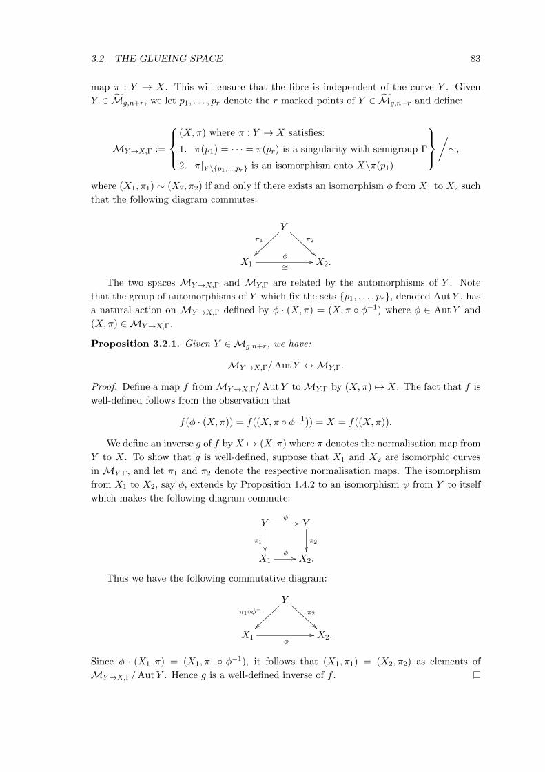
3.2. THE GLUEING SPACE 83

map π : Y → X. This will ensure that the fibre is independent of the curve Y . Given

Y ∈ Mg,n+r, we let p1, . . . , pr denote the r marked points of Y ∈ Mg,n+r and define:

MY→X,Γ :=

(X,π) where π : Y → X satisfies:

1. π(p1) = · · · = π(pr) is a singularity with semigroup Γ

2. π|Y \p1,...,pr is an isomorphism onto X\π(p1)

/∼,

where (X1, π1) ∼ (X2, π2) if and only if there exists an isomorphism φ from X1 to X2 such

that the following diagram commutes:

Yπ1

~~

π2

!!X1

φ

∼=// X2.

The two spaces MY→X,Γ and MY,Γ are related by the automorphisms of Y . Note

that the group of automorphisms of Y which fix the sets p1, . . . , pr, denoted AutY , has

a natural action on MY→X,Γ defined by φ · (X,π) = (X,π φ−1) where φ ∈ AutY and

(X,π) ∈MY→X,Γ.

Proposition 3.2.1. Given Y ∈Mg,n+r, we have:

MY→X,Γ/AutY ↔MY,Γ.

Proof. Define a map f fromMY→X,Γ/AutY toMY,Γ by (X,π) 7→ X. The fact that f is

well-defined follows from the observation that

f(φ · (X,π)) = f((X,π φ−1)) = X = f((X,π)).

We define an inverse g of f by X 7→ (X,π) where π denotes the normalisation map from

Y to X. To show that g is well-defined, suppose that X1 and X2 are isomorphic curves

in MY,Γ, and let π1 and π2 denote the respective normalisation maps. The isomorphism

from X1 to X2, say φ, extends by Proposition 1.4.2 to an isomorphism ψ from Y to itself

which makes the following diagram commute:

Y

π1

ψ // Y

π2

X1φ // X2.

Thus we have the following commutative diagram:

Yπ1φ−1

~~

π2

!!X1

φ// X2.

Since φ · (X1, π) = (X1, π1 φ−1), it follows that (X1, π1) = (X2, π2) as elements of

MY→X,Γ/AutY . Hence g is a well-defined inverse of f .


We now describe the space MY→X,Γ algebraically.

Definition 3.2.2. Let Γ be the semigroup of an r-branched curve singularity with con-

ductor (c1, . . . , cr). The semigroup of a C-subalgebra of⊕r

i=1 C[[ti]]/(tcii ) is the set

v(R) ∪ (n1, . . . , nr) ∈ Nr | ni ≥ ci, where v is the map defined in Section 2.2.1 sending

an r-tuple of power series to the r-tuple of their orders.

We define:

RΓ :=

C-subalgebras of

r⊕i=1

C[[ti]]/(tcii )

with semigroup Γ

.

Remark 3.2.3. Since a C-subalgebra in RΓ contains the ideal (tc11 , . . . , tcrr ), there is a

one-to-one correspondence between elements of RΓ and C-subalgebras of⊕r

i=1 C[[ti]]/(tcii )

with semigroup Γ. We will use both descriptions interchangeably.

Proposition 3.2.4. Let Y ∈ Mg,n+r and let Γ be the semigroup of an r-branched curve

singularity. Then there is a natural bijection:

MY→X,Γ ↔ RΓ.

Remark 3.2.5. This proposition implies that the space MY→X,Γ is independent of the

normalisation Y .

We will prove this proposition in the case r = 1 for ease of notation, but the proof also

holds in the case when r > 1. We let p ∈ Y denote the corresponding marked point, i.e.

the preimage of the singularity of X under the normalisation map π.

Proof of Proposition 3.2.4. Since Y is smooth at p, we have that OY,p ∼= C[[t]]. We fix this

isomorphism and identify the two rings throughout the proof. Given (X,π) ∈ MY→X,Γ,

we can therefore identify OX,π(p) as a subring of C[[t]] via the induced inclusion

π∗ : OX,π(p) → OY,p.

(→) Consider the following map:

F :MY→X,Γ → RΓ

(X,π) 7→ π∗(OX,π(p)/(t

c))⊆ C[t]/(tc).

To show that this map is well-defined, suppose that (X1, π1) = (X2, π2) in MY→X,Γ.

Then there exists an isomorphism φ from X1 to X2 such that the following diagram

commutes:

Yπ1

~~

π2

!!X1

φ

∼=// X2.

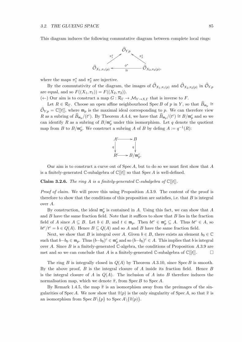
3.2. THE GLUEING SPACE 85

This diagram induces the following commutative diagram between complete local rings:

OY,p

OX1,π1(p)

π∗1::

OX2,π2(p),φ∗

∼=oo

π∗2dd

where the maps π∗1 and π∗2 are injective.

By the commutativity of the diagram, the images of OX1,π1(p) and OX2,π2(p) in OY,pare equal, and so F ((X1, π1)) = F ((X2, π2)).

(←) Our aim is to construct a map G : RΓ →MY→X,Γ that is inverse to F .

Let R ∈ RΓ. Choose an open affine neighbourhood SpecB of p in Y , so that Bmp∼=

OY,p = C[[t]], where mp is the maximal ideal corresponding to p. We can therefore view

R as a subring of Bmp/(tc). By Theorem A.4.4, we have that Bmp/(t

c) ∼= B/mcp and so we

can identify R as a subring of B/mcp under this isomorphism. Let q denote the quotient

map from B to B/mcp. We construct a subring A of B by defing A := q−1(R):

A

q

// B

q

R // B/mc

p.

Our aim is to construct a curve out of SpecA, but to do so we must first show that A

is a finitely-generated C-subalgebra of C[[t]] so that SpecA is well-defined.

Claim 3.2.6. The ring A is a finitely-generated C-subalgebra of C[[t]].

Proof of claim. We will prove this using Proposition A.3.9. The content of the proof is

therefore to show that the conditions of this proposition are satisfies, i.e. that B is integral

over A.

By construction, the ideal mcp is contained in A. Using this fact, we can show that A

and B have the same fraction field. Note that it suffices to show that B lies in the fraction

field of A since A ⊆ B. Let b ∈ B, and t ∈ mp. Then btc ∈ mcp ⊆ A. Thus btc ∈ A, so

btc/tc = b ∈ Q(A). Hence B ⊆ Q(A) and so A and B have the same fraction field.

Next, we show that B is integral over A. Given b ∈ B, there exists an element b0 ∈ Csuch that b−b0 ∈ mp. Thus (b−b0)c ∈ mc

p and so (b−b0)c ∈ A. This implies that b is integral

over A. Since B is a finitely-generated C-algebra, the conditions of Proposition A.3.9 are

met and so we can conclude that A is a finitely-generated C-subalgebra of C[[t]].

The ring B is integrally closed in Q(A) by Theorem A.3.10, since SpecB is smooth.

By the above proof, B is the integral closure of A inside its fraction field. Hence B

is the integral closure of A in Q(A). The inclusion of A into B therefore induces the

normalisation map, which we denote π, from SpecB to SpecA.

By Remark 1.4.5, the map π is an isomorphism away from the preimages of the sin-

gularities of SpecA. We now show that π(p) is the only singularity of SpecA, so that π is

an isomorphism from SpecB\p to SpecA\π(p).


Let q 6= p be a point of SpecB and let f ∈ mcp\mq. Note that since f ∈ mc

p, f ∈ A.

By choice of f , the set SpecBf is an open neighbourhood of the point q. It is clear that

Af ⊆ Bf by the remarks following Proposition A.2.6, since A ⊆ B. Moreover, given

b ∈ B, we have that fb ∈ A since f ∈ mcp. Hence b = fb/f ∈ Af . It follows that

B ⊆ Af , and so Bf ⊆ Af . Thus we have that Af = Bf , from which we can conclude that

SpecAf ∼= SpecBf . Hence π(q) must be a smooth point of SpecA, since q is a smooth

point of SpecB. It follows that SpecA has only one singular point, at π(p), and so

SpecB\p ∼= SpecA\π(p).

We now define:

X := (Y \p t SpecA)/x ∼ π(x)

for all x ∈ SpecB\p. We also define a map π : Y → X by letting π|Y \p be the natural

inclusion of Y \p into X, and by setting π(p) = π(p).

Since the map π|Y \p is an isomorphism onto X\π(p), we have that π is an isomor-

phism away from p.

We can now define G(R) as the pair (X,π). It remains to show that (X,π) ∈MY→X,Γ.

To do so, it suffices to show that π(p) is a singularity with semigroup Γ.

By construction, OX,π(p)∼= OSpecA,π(p), which we denote by A. By Theorem A.4.4, we

have that A/mcp∼= A/mc

p, which by construction is isomorphic to R. Thus OSpecA,π(p)/mcp

has semigroup Γ, and so by definition OSpecA,π(p) itself has semigroup Γ.

Hence (X,π) ∈MY,Γ.

The fact that the maps F and G are inverse to each other follows from their construc-

tion.

The study of MY→X,Γ can, as a result of Proposition 3.2.4, be carried out purely

algebraically via the study of RΓ. We will use this set-theoretic bijection to identify

MY→X,Γ as a topological space in Remark 3.3.24.

3.3 Describing RΓ

In this section we explicitly describe RΓ in a number of cases: for plane branch semigroups

with two (Proposition 3.3.8) and three generators (Proposition 3.3.12), and in the multi-

branched case for the semigroups of the nodal singularity and of the singularity of V (y(y−xk)) where k ≥ 1 (Examples 3.3.21 and 3.3.23). Our approach is to determine so-called

normal forms of generators for any given semigroup Γ. These normal forms must satisfy

the property that any ring in RΓ has generators of this form, and two rings in RΓ are

equal if and only if the normal forms of their generators are equal. Finally, we show that

there is a natural map from RΓ to MΓ given by identifying isomorphic rings in RΓ. We

explicitly compute this map in the case of the semigroup Γ = 〈3, 7〉 (Example 3.3.25).

We will study RΓ in the case of plane curve singularities, as we did in the case of the

Zariski moduli space in Chapter 2. We let Γ denote the semigroup of an r-branched plane

curve singularity, with conductor (c1, . . . , cr).

3.3. DESCRIBING RΓ 87

Complete local rings of plane curve singularities are characterised by the property that

they have only two generators when identified as C-subalgebras of⊕r

i=1 C[[ti]], where r

denotes their number of branches. From here on, we consider only the subset of RΓ

consisting of C-subalgebras with two generators. For ease of reference, we relabel this

subset of RΓ, and so we assume that all rings R ∈ RΓ are generated by two elements.

Notation 3.3.1. A ring R ∈ RΓ consists of a C-subalgebra of⊕r

i=1 C[[ti]]/(tcii ) with semi-

group Γ. Given R ∈ RΓ, we let x(t) := (x1(t1), . . . , xr(tr)) and y(t) := (y1(t1), . . . , yr(tr))

denote the generators of R, where xi(ti), yi(ti) ∈ C[[ti]]/(tcii ).

The generators x(t) and y(t) of a ring R ∈ RΓ can be viewed as a parametrisation by

considering the map:

ϕ : C[[x, y]]→r⊕i=1

C[[ti]]

x 7→ x(t)

y 7→ y(t).

A parametrisation of the singularity is then given by ϕ = (xi(ti), yi(ti))ri=1, using the

notation from Notation 2.3.2.

Conversely, any parametrisation ϕ = (xi(ti), yi(ti))ri=1 of a plane curve singularity

with semigroup Γ induces a ring R ∈ RΓ obtained by taking the C-subalgebra generated

by x(t) := (x1(t1), . . . , xr(tr)) and y(t) := (y1(t1), . . . , yr(tr)).

Two such parametrisations ϕ and ϕ′ determine the same ring in RΓ if there exists an

automorphism σ ∈ AutC[[x, y]] such that the following diagram commutes:

C[[x, y]]ϕ // Or

C[[x, y]].

σ

OO

ϕ′

;;

With this perspective, the problem of describing RΓ can be reformulated in the fol-

lowing way.

Problem 3.3.2. For any given plane curve semigroup Γ, identify the simplest possible

form of generators x(t) and y(t), called “normal forms”, such that:

(i) any ring in RΓ admits generators of this form,

(ii) any ring with generators of this form has semigroup Γ, and

(iii) two rings in RΓ are equal if and only the normal forms of their generators are equal.

We will solve this problem in the case of irreducible plane curve singularities in Section

3.3.1. For multi-branched singularities, we will solve the problem in two particular cases

in Section 3.3.2.


3.3.1 Irreducible plane curve singularities

We start by solving Problem 3.3.2 in the case of plane branch singularities. Let Γ =

〈v0, . . . vg〉 denote a plane branch semigroup with conductor c.

For plane branch semigroups, the solution consists of two parts. In Proposition 3.3.4,

we identify so-called reduced forms of generators with respect to Γ, so that any ring in

RΓ admits generators in reduced forms, and two rings in RΓ are equal if and only if the

reduced forms of their generators are equal.

We then identify conditions on the reduced form of these generators which ensure

that they generate a ring with semigroup Γ. Generators in reduced form satisfying these

conditions are the normal forms of generators with respect to Γ that are referred to in

Problem 3.3.2. In Proposition 3.3.8 we will explicitly give the normal forms of generators

in the case where Γ is generated by two elements.

In the case where Γ is generated by three or more elements, Proposition 3.3.12 will

give the conditions on the reduced forms of generators with respect to Γ which ensure

that they generate a ring with semigroup Γ. We will then be able to illustrate with some

examples how these conditions allow us to explicitly obtain normal forms of generators for

a given semigroup with three generators.

Before identifying the reduced forms of generators for plane branch semigroups, we

give a characterisation of plane branch semigroups which we will need in the proofs of

Proposition 3.3.8 and Proposition 3.3.12. Recall from Proposition 2.2.17 that any numer-

ical semigroup with a conductor is the semigroup of a curve singularity. Nevertheless, not

every numerical semigroup arises as the semigroup of a plane curve singularity. The fol-

lowing proposition gives the necessary and sufficient conditions for a numerical semigroup

to be the semigroup of a plane branch singularity.

Proposition 3.3.3 (Characterisation of plane branch semigroups [BDF03, Proposition

4.8]). Let Γ = 〈v0, . . . , vg〉 be a numerical semigroup, so that gcd(v0, . . . , vg) = 1. Let

e0 = v0 and let ei = gcd(v0, . . . , vi) for all i = 1, . . . , g. Then Γ is a plane branch

semigroup if and only if the following two conditions hold:

(i) e0 > e1 > . . . > ek = 1,

(ii) vi > lcm(ei−2, vi−1) for i = 2, ..., k.

The proof of the necessity of these conditions relies on a formula proved by Zariski in

[Zar06, Theorem 3.9]. It relates the characteristic exponents of a singularity, introduced

in Remark 2.3.9, to its semigroup. The proof of their sufficiency is obtained by showing

that the complete local ring:

C[[tv0 , tv1 + tv1+v2−lcm(e0,v1) + · · ·+ tv1+···+vg−(lcm(e0,v1)+···+lcm(eg−2,vg−1)]]

has semigroup Γ [BDF03].

We can now describe the reduced forms of generators for any given plane branch

semigroup Γ.


Proposition 3.3.4. Let q1, . . . , qr denote the elements of N\Γ that are larger than v0. If

there is an element qi larger than v1, then let j be the smallest integer such that qj > v1.

Suppose that R ∈ RΓ. Then R admits generators of the form:

x(t) = tv0 + a1tq1 + · · ·+ art

qr , and

y(t) =

tv1 + bjt

qj + · · ·+ brtqr if j exists

tv1 otherwise,

where ai, bi ∈ C. Moreover, these generators are unique.

Definition 3.3.5. We call these generators the reduced forms of generators with respect

to the semigroup Γ.

Proof of Proposition 3.3.4. Let R = C[[x(t), y(t)]] ∈ RΓ. Since R ⊆ C[[t]]/(tc), the degrees

of the polynomials x(t) and y(t) must be less than c. The ring R has semigroup Γ, so it

must contain elements of orders v0 and v1. These are the smallest elements of Γ, so the

generators x(t) and y(t) must have these orders. Without loss of generality, we assume

that x(t) has order v0 and that y(t) has order v0. Thus:

x(t) = d0tv0 + · · ·+ dc−1t

c−1 and

y(t) = e0tv0 + · · ·+ ec−1t

c−1

for some di, ei ∈ C. By scaling x(t) and y(t), which preserves the ring, we can assume that

d0 = e0 = 1.

Let p1, . . . , ps = a ∈ Γ | v0 < a < c for all i, where pi < pi+1 for all i = 1, . . . , g−1.

For each pi, there exists a monic polynomial fi(t) ∈ R such that ord fi(t) = pi. We can

remove the term dpstps appearing in x(t) by subtracting from it dpsfps(t). Then, we can

remove the term dps−1tps−1 from x(t) by subtracting dps−1fps−1(t). Proceeding in this way,

we can eliminate every power pi appearing in x(t) to obtain a polynomial in R of the form:

tv0 + a1tq1 + · · ·+ art

qr

for some ai ∈ C.

The same process can be applied to the generator y(t). In this case, we let p1, . . . , psdenote the elements of Γ lying strictly between v1 and c. We eventually obtain a polynomial

in R of the form:

tv1 + bjtqj + · · ·+ brt

qr

for some bi ∈ C.

By construction, both these polynomials generate R. We relabel these generators as

x(t) and y(t) for ease of notation.

It remains to be shown that these are the unique generators of this form. Suppose

that R contains another element x′(t) 6= x(t) of the form tv0 + a1tq1 + · · · + art

qr . Then

the order of x′(t) − x(t) is strictly greater than v0, and must therefore be an element of

q1, . . . , qr since x′(t) 6= x(t). This contradicts the assumption that R has semigroup Γ,

since qi 6= Γ for all i. For the same reason, R cannot contain another element y′(t) of the

form tv1 + bjtqj + · · · bjtqj . Thus the generators x(t) and y(t) of R constructed above are

unique.


Notation 3.3.6. From here on, when we write R = C[[x(t), y(t)]] ∈ RΓ, we will always

assume that x(t) and y(t) are in reduced form with respect to Γ.

In order to solve Problem 3.3.2, given x(t) and y(t) in reduced form with respect to Γ,

we must determine sufficient and necessary conditions on their coefficients which ensure

that they generate a ring with semigroup Γ.

The following example shows why this is in general a non-trivial problem.

Example 3.3.7. Let Γ = 〈4, 6, 13〉. The gaps of Γ that are larger than 4 consists of the

set 5, 7, 9, 11, 14. Hence by Proposition 3.3.4, any ring in RΓ admits a unique set of

generators of the form:

x(t) = t4 + a5t5 + a9t

9 + a11t11 + a14t

14 and

y(t) = t6 + b7t7 + b9t

9 + b11t11 + b14t

14

for some ai, bi ∈ C. Consider the generators x(t) = t4 and y(t) = t6 + t9, which are of the

above form. We have:

y(t)2 − x(t)3 = (t6 + t9)2 − (t4)3 = 2t15.

Hence 15 ∈ Γ, and so R = C[[x(t), y(t)]] /∈ Γ.

As this example shows, the reduced forms of generators with respect to a semigroup

Γ may not generate a ring with semigroup Γ. Thus we must determine sufficient and

necessary conditions on the coefficients of the reduced forms of the generators which will

ensure that they generate a ring with semigroup Γ.

In the case of semigroups Γ with two generators, the conditions are trivial: any pair

of generators in reduced form with respect to Γ generate a ring with semigroup Γ.

3.3.1.1 Semigroups with two generators

Proposition 3.3.8. Let Γ = 〈v0, v1〉 be the semigroup of a plane branch singularity.

Then any generators x(t) and y(t) in reduced form with respect to Γ generate a ring with

semigroup Γ.

Proof. Since Γ has a conductor, v0 and v1 must be relatively prime by Proposition 3.3.3.

Let R = C[[x(t), y(t)]], and let ΓR denote the semigroup of R. Then 〈v0, v1〉 ⊂ ΓR, since

x(t) and y(t) have orders v0 and v1 respectively.

Given that ΓR is also a plane branch semigroup, then by Proposition 3.3.3 it cannot

contain any integer n /∈ 〈v0, v1〉 less than c. Indeed, if it did contain such an element,

then we would have gcd(v0, v1, v2) = gcd(v0, v1, v2, n) = 1, contradicting condition (i) of

Proposition 3.3.3.

The above proposition allows us to explicitly describe the space RΓ for plane branch

semigroups with two generators.


Corollary 3.3.9. Let Γ = 〈v0, v1〉 be a plane branch semigroup. Suppose that q1, . . . , qrare the gaps of Γ that are greater than v1. Let j be the smallest index such that qj > β.

Then:

RΓ ↔

A2r−j+1 if j exists,

Ar otherwise.

Proof. By Proposition 3.3.4 we know that any ring in RΓ can be written in a unique way

in the form R = C[[tv0 + a1tq1 + · · · + art

qr , tv1 + bjtqj + · · · + brt

qr ]] for some ai, bi ∈ C.

Note that if no such j exists, then we assume that all of the coefficients bi are zero.

Let Φ : RΓ → A2r−j+1 be defined by:

C[[tv0 + a1tq1 + · · ·+ art

qr , tv1 + bjtqj + · · ·+ brt

qr ]] 7→

(a1, . . . , ar, bj , . . . , br) if j exists,

(a1, . . . , ar) otherwise.

This map is injective by Proposition 3.3.4. It is surjective by Proposition 3.3.8, since

C[[tv0 + a1tq1 + · · · + art

qr , tv1 + bjtqj + · · · + tqr ]] has semigroup equal to Γ for any

(a1, . . . , ar, bj , . . . , br) ∈ A2r−j+1, or any (a1, . . . , ar) ∈ Ar if j doesn’t exist. Thus:

RΓ ↔

A2r−j+1 if j exists

Ar otherwise.

3.3.1.2 Semigroups with three generators

We now address Problem 3.3.2 in the case where Γ is a plane branch semigroup generated

by three elements. We let Γ = 〈v0, v1, v2〉 denote such a semigroup.

As seen in Example 3.3.7, in this case we must identify conditions on the coefficients

of the reduced forms of generators with respect to Γ which ensure that they generate a

ring with semigroup Γ. We do so in Proposition 3.3.12, which states that generators x(t)

and y(t) in reduced form with respect to Γ generate a ring of semigroup Γ if and only if

an appropriately defined “reduced form” of y(t)k1 − x(t)k0 has order v2, where k0 and k1

are integers satisfying k0v0 = k1v1 = lcm(v0, v1).

We start by defining this reduced form, which should not be mistaken for the reduced

forms of generators with respect to Γ from Definition 3.3.5.

Note that the algorithm which we describe below holds for any plane branch semigroup,

not just those with three generators, and so we describe it for an arbitrary plane branch

semigroup.

Algorithm 3.3.10 (Reduction algorithm). Let Γ = 〈v0, v1, . . . , vg〉 and suppose that

R = C[[x(t), y(t)]] ∈ RΓ. Moreover, let f(t) ∈ R be a monic polynomial of order n. Note

that n < c since R ⊆ C[[t]]/(tc).

Let p1, . . . , pr denote the elements of N\〈v0, v1〉 such that v0 < pi < c for all i. Let

s1, . . . , st denote the elements of 〈v0, v1〉 such that n < si < c for all i. For each i, there

exists some k and l such that x(t)ky(t)l ∈ R has order si. We choose k and l such that

l is minimal. Note that l is always strictly less than k1, since k1v1 = k0v0. Indeed, if


v0k + v1l = si and l > k1, then we also have 2v0k0 + (l − k1)v1 = si. We can continue

subtracting k0v0 until the coefficient in front of v1 is less than k1.

Choosing l to be minimal ensures that the choice of fi(t) is unique. Take i = 1, and

let a1 be the coefficient in front of ts1 in f(t). We can eliminate this power from f by

subtracting a1f1(t).

Let a2 be the coefficient in front of ts2 in f(t) − a1f1(t). This power can be removed

by subtracting a2f2(t) from f(t)−a1f1(t). Proceeding in this way, we obtain a unique set

of elements a1, . . . , ar such that f(t)− (∑s

i=1 aifi(t)) is of the form tn + a1tp1 + · · ·+ art

pr

for some ai ∈ C.

Definition 3.3.11. Given an element f(t) ∈ R with ord f(t) < c, the polynomial obtained

from the above algorithm is called the reduced form of f with respect to 〈v0, v1〉, and we

denote it red〈v0,v1〉 f(t).

In Example 3.3.17, we take Γ = 〈4, 6, 15〉 and compute the reduced form of y(t)2−x(t)3

with respect to 〈4, 6〉, where x(t) = t4 and y(t) = t6 + t9.

The following proposition will provide us with necessary and sufficient conditions for

the reduced form of generators with respect to Γ to generate a ring with semigroup Γ.

Proposition 3.3.12. Let Γ = 〈v0, v1, v2〉 be a plane branch semigroup and let k0 and k1

be natural numbers satisfying k0v0 = k1v1 = lcm(v0, v1). Then R = C[[x(t), y(t)]] has

semigroup Γ if and only if:

red〈v0,v1〉

(y(t)k1 − x(t)k0

)= v2.

Before proving this result, we give the following definitions which will be needed for

the proof.

Definition 3.3.13. Let R = C[[x(t), y(t)]] ∈ RΓ, where Γ = 〈v0, . . . , vg〉. Given a mono-

mial axiyj ∈ C[[x, y]] where a ∈ C∗, we define its weighted degree d to be the integer

d := v0i+ v1j. The weighted degree d of a power series g(x, y) ∈ C[[x, y]] is the minimum

weighted degree d of the monomials appearing in g(x, y). We write d := deg g(x, y).

The order of g(x, y) with respect to R, denoted ord g(x, y), is the order of g(x(t), y(t)) ∈C[[t]].

A polynomial g ∈ C[[x, y]] is deceptive in R if ordt g(x, y) 6= deg g(x, y).

Remark 3.3.14. Any monomial xiyj ∈ C[[x, y]] is not deceptive in R, since the absence

of any addition or subtraction prevents the cancellation of the lowest order power of xiyj .

Example 3.3.15. Consider the ring R = C[[t2+t3, t5]] ∈ R〈2,5〉, and let x = t2 and y = t3.

We have that deg(y2 − x5) = 10, while ordt(y2 − x5) = ordt(t

10 − t10 − 5t11 − · · · ) = 11.

Thus the element y2 − x5 ∈ C[[x, y]] is deceptive in R.


Proof. We start by showing that ifR = C[[x(t), y(t)]] ∈ RΓ, then red〈v0,v1〉(y(t)k1 − x(t)k0

)=

v2.


Note that ord red〈v0,v1〉(yk1 − xk0

)/∈ 〈v0, v1〉, by definition of red〈v0,v1〉(y

k1−xk0). Thus

we cannot have that ord red〈v0,v1〉(yk1 − xk0

)< v2, since v2 is the smallest element of Γ

that does not lie in 〈v0, v1〉 by virtue of the set v0, v1, v2 being a set of minimal generators

for Γ.

We therefore suppose, in order to reach a contradiction, that:

ord red〈v0,v1〉

(γk11 − γ

k00

)> v2.

Since v2 ∈ Γ, there exists a power series q(x, y) ∈ C[[x, y]] such that ord q(x, y) = v2. We

can without loss of generality assume that q(x, y) is a polynomial, since q(x, y) can have

only a finite number of monomials of order less than v2. Thus we can write:

q(x, y) = q0(x) + q1(x)y + · · ·+ qk(x)yk

for some k ∈ N, where qi(x) ∈ C[x] for all i.

We now show that we can assume without loss of generality that k < k1. Indeed,

suppose that k ≥ k1. By Algorithm 3.3.10,

red〈v0,v1〉

(yk1 − xk0

)= y(t)k1 − x(t)k0 − F (x, y)

for some polynomial F (x, y) with y degree strictly less than k1. Thus we can remove from

q(x, y) the term qk(x)yk by subtracting qk(x)yk−k1(red〈v0,v1〉

(yk1 − xk0

))from it. This

subtraction does not change the order of the polynomial since by assumption:

ord red〈v0,v1〉

(yk1 − xk0

)> v2.

Thus, we may assume without loss of generality that:

q(x, y) = q0(x) + · · ·+ qk1−1(x)yk1−1

where qi ∈ C[[x]] for all i.

Since the order of any xiyj in q(x, y) is an integer in 〈v0, v1〉, q(x, y) must be deceptive

for it to have order v2 /∈ 〈v0, v1〉. In particular, there must be at least two monomials,

which we denote aijxiyj and ai′j′x

i′yj′, in q(x, y) with equal order. Thus we have:

v0i+ v1j = v0i′ + v1j

′. (3.1)

For this equation to hold, we must either have i < i′ and j > j′, or i > i′ and j < j′.

Since the argument is the same in both cases, we assume without loss of generality that

i < i′ and that j > j′. Hence we must have:

v1(j − j′) = v0(i− i′).

The smallest value of n such that nv1 = mv0 for some m ∈ N is k1. Nevertheless, since

by assumption j < k1, we also have j − j′ < k1. Thus (3.1) cannot hold and so we cannot

have that ord(red〈v0,v1〉(yk1 − xk0)) > v2. It follows that ord(red〈v0,v1〉(γ

k11 − γ

k00 )) = v2.

It remains for us to show that if ord(red〈v0,v1〉(γk11 −γ

k00 )) = v2, then R = C[[x(t), y(t)]]

has semigroup Γ. Let ΓR denote the semigroup of R. By assumption, 〈v0, v1, v2〉 ⊆ ΓR.

Since gcd(v0, v1, v2) = 1, then by Proposition 3.3.3 we must have that ΓR = 〈v0, v1, v2〉 =

Γ.


The following examples illustrate how the above proposition allows us to explicitly

describe RΓ for any plane branch semigroup Γ with three generators.

Example 3.3.16. Let Γ = 〈4, 6, 13〉. The conductor of Γ is 16 and the gaps of Γ greater

than 4 are: 5, 7, 9, 11, 15. The reduced forms of generators x(t) and y(t) with respect to

Γ are:

x(t) = t4 + a5t5 + a7t

7 + a9t9 + a11t

11 + a15t15 and

y(t) = t6 + b7t7 + b9t

9 + b11t11 + b15t

15.

In this case the integers k0 and k1 from Proposition 3.3.12 are equal to 3 and 2 respectively,

since lcm(4, 6) = 12. To apply Proposition 3.3.12, we must compute red〈4,6〉(y(t)2−x(t)3).

We have:

y(t)2 − x(t)3 = (t6 + b7t7 + · · · )2 − (t4 + a5t

5 + · · · )3

= t12 + 2b7t13 − t12 − 3a5t

13 + higher order terms (h.o.t.)

= (2b7 − 3a5)t13 + h.o.t..

Since 13 /∈ 〈4, 6〉, the corresponding power is not removed from red〈4,6〉(y(t)2 − x(t)3)

and so we have:

red〈4,6〉(y(t)2 − x(t)3) = (2b7 − 3a5)t13 + h.o.t..

Let R = C[[x(t), y(t)]]. By Proposition 3.3.12, R has semigroup Γ if and only if:

ord(red〈4,6〉(y(t)2 − x(t)3)

)= 13,

that is if and only if b7 6= (3/2)a5.

Hence we can conclude that:

RΓ ↔ C[[x(t), y(t)]] | b7 6= (3/2)a5↔ A1\0 × A8.

Example 3.3.17. Let Γ = 〈4, 6, 15〉. The conductor of Γ is 18 and the gaps of Γ greater

than 4 are: 5, 7, 9, 11, 13, 17. The reduced forms of generators x(t) and y(t) with respect

to Γ are:

x(t) = t4 + a5t5 + a7t

7 + a9t9 + a11t

11 + a13t13 + a17t

17 and

y(t) = t6 + b7t7 + b9t

9 + b11t11 + b13t

13 + b17t17.

Again, k0 = 3 and k1 = 2, and we have:

y(t)2 − x(t)3 = (t6 + b7t7 + b9t

9 + · · · )2 − (t4 + a5t5 + a7t

7 · · · )3

= t12 + 2b7t13 + b27t

14 + 2b9t15 − t12 − 3a5t

13 − 3a25t

14 − 3a7t15 + h.o.t.

= (2b7 − 3a5)t13 + (b27 − 3a25)t14 + (2b9 − 3a7)t15 + h.o.t..

The first few terms of red〈4,6,〉(y(t)2 − x(t)3) can now be computed. Since 13 /∈ 〈4, 6〉,this power is not removed when passing to the reduced form of y(t)2 − x(t)3, by applying


Algorithm 3.3.10. The power 14 however does lie in 〈4, 6, 〉, and hence must be removed

by subtracting from y(t)2 − x(t)3 the expression (b27 − 3a25)x(t)2y(t). We have:

x(t)2y(t) = (t4 + a5t5 + a6t

6 + · · · )2(t6 + b7t7 + · · · )

= (t8 + 2a5t9 + (a2

5 + 2a6)t10 + · · · )(t6 + b7t7 + · · · )

= t14 + (2a5 + b7)t15 + · · · .

Thus we have:

y(t)2 − x(t)3 − (b27 − 3a25)x(t)2y(t) = (2b7 − 3a5)t13 + (2b9 − 3a7 − (b27 − 3a2

5)(2a5 + b7))t15

+ h.o.t.

= (2b7 − 3a5)t13 + (2b9 − 3a7 − 2b27a5 − b37 + 6a35 + 3a2

5b7)t15

+ h.o.t..

Hence:

red〈4,6,〉(y(t)2−x(t)3) = (2b7− 3a5)t13 + (2b9− 3a7− 2b27a5− b37 + 6a35 + 3a2

5b7)t15 + h.o.t..

By Proposition 3.3.12, R = C[[x(t), y(t)]] has semigroup Γ if and only if:

ord(red〈4,6,〉(y(t)2 − x(t)3)

)= 15,

that is if and only if:

b9 6= (1/2)(−3a7 − 2b27a5 − b37 + 6a35 + 3a2

5b7).

Hence we can conclude that:

RΓ ↔C[[x(t), y(t)]] | b9 6= (1/2)(−3a7 − 2b27a5 − b37 + 6a3

5 + 3a25b7).

↔ A1\0 × A10.

In light of the above two examples, a logical question to ask is whether the moduli

space RΓ is always of the form A1\0 × AN for some N ∈ N, when Γ is generated by

three elements. Extensive computation suggests that this may indeed be the case. I have

attempted to prove this in general but the reasoning is lengthy and convoluted. For this

reason it has not been included.

3.3.1.3 Towards a general solution

In the case where Γ = 〈v0, . . . , vg〉 is an arbitrary plane branch semigroup, we can gen-

eralise the proof of Proposition 3.3.12 to obtain a solution to Problem 3.3.2, given in

Proposition 3.3.19. Its statement relies on a generalisation of Algorithm 3.3.10.

Algorithm 3.3.18 (Generalisation of Algorithm 3.3.10). Let Γ = 〈v0, v1, . . . , vg〉 with

conductor c and let R = C[[x(t), y(t)]] ∈ RΓ. Let f(t) ∈ R be a monic polynomial of order

n < c. We can apply the same procedure to f(t) as described in Algorithm 3.3.10, except

instead of removing from f(t) only the powers of t that lie in 〈v0, v1〉, we can remove, for

a fixed j ≤ g, all powers of t that lie in 〈v0, . . . , vj〉. We call the resulting polynomial the

reduced form of f with respect to 〈v0, . . . , vj〉, and denote it red〈v0,...,vj〉 f(t).


Proposition 3.3.19. Let ei = gcd(v0, . . . , vi). Furthermore, let (m0,m1, . . . ,mi−1) be

a solution in the positive integers to the diophantine equation m0v0 + · · · + mi−1vi−1 =

lcm(ei−2, vi), where the integers mi are minimised, starting from i− 1.

Suppose that R = C[[x(t), y(t)]] ∈ RΓ, where x(t) and y(t) are in reduced form, and

let:

γ2(t) = red〈v0,v1〉

(y(t)k1 − x(t)k0

)where k1v1 = k0v0 = lcm(v0, v1),

γ3(t) = red〈v0,v1,v2〉

(γ2(t)k2 − γ0(t)m0γ1(t)m1

)where k2v2 = lcm(gcd(v0, v1), v2),

...

γg(t) = red〈v0,...,vg−1〉

(γg−1(t)kg−1 − γm0

0 (t) · · · γg−2(t)mg−2

)where kg−1vg−1 = lcm(eg−2, vg−1).

Then R ∈ RΓ if and only if ord γi(t) = vi for all i = 2, . . . , g.

3.3.2 Multi-branched singularities

We now address Problem 3.3.2 in the context of semigroups of multi-branched plane curve

singularities. More precisely, we describe RΓ in the following two cases:

1) The semigroup Γ of the nodal singularity C[[x, y]]/(y(y − x)).

2) The semigroup Γ of the singularity C[[x, y]]/(y(y − xk)) for k ≥ 1.

Remark 3.3.20. Suppose that Γ is the semigroup of an r-branched curve singularity with

conductor (c1, . . . , cr) and let R ∈ RΓ, where we view R as a C-subalgebra of⊕r

i=1 C[[ti]]

by applying Remark 3.2.3. Then since R has semigroup Γ, for any element (n1, . . . , nr) ∈ Γ

there exists an element of R with this order.

In the case where Γ is a unibranch semigroup with conductor c, it follows that (tc) ⊆ R,

as seen in Remark 3.3.20. The same holds true for multi-branched singularities: if R ∈ RΓ,

then (tc1)⊕ · · · ⊕ (tcr) ⊆ R.

In other words, if R ∈ RΓ then given (n1, . . . , nr) ∈ Nr with ni ≥ ci for all i, R contains

any element (f1(t1), . . . , fr(tr)) ∈⊕r

i=1 C[[ti]] of order (n1, . . . , nr) with ni ≥ ci for all i,

not just one element of order (n1, . . . , nr).

The proof of this is straightforward but somewhat lengthy. The main idea can be

illustrated using two-branched semigroups.

Given a semigroup Γ ⊆ N2 with conductor (c1, c2) and R ∈ RΓ, to show that (tc1) ⊕(tc2) ⊆ R it suffices to show that for any (n1, n2) ∈ N2 with n1 ≥ c1 and n2 ≥ c2, the

elements (tn11 , 0) and (0, tn−2

2 ) both lie in R.

Since (n1, n2) ∈ Γ, there exists an element in R of this order, which we can assume is of

the form f(t) = (tn11 +an1+1t

n1+11 + · · · , bn2t

n22 + · · · ), where bn2 6= 0. Since (n1 + 1, bn2) is

also in Γ, there exists an element in R of this order. Subtracting an appropriate multiple of

it from f(t) yields (tn11 + · · · , bn2+1t

n2+12 + · · · ). Proceeding in this way, we can iteratively

remove all powers appearing in the second power series of f(t) since we can use infinite

power series and obtain an element (tn11 , 0) ∈ R. By symmetry, we can also obtain (0, tn2

2 ) ∈R.


1 2 3 4 5 6

0

1

2

3

4

5

6

7

(a) The semigroup of the nodal singu-

larity V (y(y − x)).

1 2 3 4 5 6

0

1

2

3

4

5

6

7

(b) The semigroup of the tacnode sin-

gularity V (y(y − x2)).

1 2 3 4 5 6

0

1

2

3

4

5

6

7

(c) The semigroup of the oscnode sin-

gularity V (y(y − x3)).

Figure 3.1: Semigroups of double-branched plane curve singularities.

Example 3.3.21. Let O = C[[x, y]]/(y(y − x)). We start by determining the semigroup

Γ ⊆ N2 of the nodal singularity O. An inclusion ϕ : C[[x, y]]/(y(y − x)) → C[[t]] ⊕ C[[t]]

is given by:

x 7→ (t, 0), and

y 7→ (t, t).

The semigroup Γ of O contains all pairs (n,m) for n,m ≥ 1. Thus the conductor of Γ is

the element (1, 1) ∈ N2. The semigroup Γ is depicted in Figure 3.1a.

Our aim is to describe the set

RΓ =

C[[x(t), y(t)]] ⊆ C[[t]]⊕ C[[t]]

with semigroup Γ

,

where x(t) = (x1(t), x2(t)) and y(t) = (y1(t), y2(t)).

By Remark 3.3.20, a ring R = C[[x(t), y(t)]] ∈ RΓ must contain the ideal (t) ⊕ (t).

Thus R must contain both the elements (t, 0) and (0, t). Without loss of generality we can


assume that these are the generators of R, since the generators of R must correspond to

two linearly independent pairs (x1(t), x2(t)) and (y1(t), y2(t)) of order (1, 1).

Thus any ring R ∈ RΓ is equal to a ring with generators (t, 0) and (0, t) and so in this

case the set RΓ is trivial:

RΓ = C[[(t, 0), (0, t)]] = ∗.

This solves Problem 3.3.2: there is a unique normal of generators with respect to Γ,

given by x(t) = (t, 0) and y(t) = (0, t).

Example 3.3.22. Let O = C[[x, y]]/(y(y − x2)). An inclusion ϕ of O into C[[t]] ⊕ C[[t]]

is given by:

x 7→ (t, t), and

y 7→ (t2, 0).

The semigroup Γ of this singularity is depicted in Figure 3.1b. It has conductor (2, 2),

and also contains the point (1, 1).

Suppose that R = C[[x(t), y(t)]] ∈ RΓ, where we let x(t) = (x1(t), x2(t)) and y(t) =

(y1(t), y2(t)). The ring R must contain an element of order (1, 1), which is the smallest

element of Γ. Thus we can assume that x(t) has this order.

Since (2, 2) is the conductor of Γ, we can remove all powers of the two power series

defining x(t) that are larger than 2. In this way, we have that x(t) = (at, bt) for some

a, b ∈ C∗. By scaling x(t), we can assume that x(t) = (t, ct) for some c ∈ C∗. We then

have that x(t)2 = (t2, c2t2). Since (2, 2) is the conductor of Γ, the pair (t2, 0) must lie in

R. However, the pair (t2, 0) is not a multiple of x(t)2 and hence we can assume without

loss of generality that y(t) = (t2, 0).

In this way, any ring R ∈ RΓ is equal to a ring with semigroup Γ generated by (t, ct)

and (t2, 0) for some c ∈ C∗. Note that two such rings with different values of c are

necessarily distinct, since (t, dt) /∈ C[[(t, ct), (t2, 0)]] for d 6= c. Thus we have shown that:

RΓ =C[[(t, ct), (t2, 0)]] | c ∈ C∗

↔ C∗.

Hence the normal forms of generators with respect to Γ are: x(t) = (t, ct) for some

c ∈ C∗ and y(t) = (t2, 0). This solves Problem 3.3.2 for this particular semigroup Γ.

We can now generalise the above example to the case where O = C[[x, y]]/(y(y−xk)).

Example 3.3.23. Let O = C[[x, y]]/(y(y − xk)). An inclusion ϕ of O into C[[t]] ⊕ C[[t]]

is given by:

x 7→ (t, t), and

y 7→ (0, tk).

The semigroup Γ of O has conductor (k, k) and also contains (n, n) for any 1 ≤ n ≤ k.

The semigroup Γ is depicted in Figure 3.1c, in the case where k = 3.

Let R = C[[x(t), y(t)]] ∈ RΓ, where x(t) = (x1(t), x2(t)) and y(t) = (y1(t), y2(t)).

The ring R must contain an element of order (1, 1), which we can assume is of the form


(t + a2t2 + · · · + ak−1t

k−1, b1t + b2t2 + · · · + bk−1t

k−1) for some ai, bi ∈ C with b1 6= 0.

Note that we need only consider polynomials of degree less than k, since Γ has conductor

(k, k) and hence all higher powers of t can be removed. Without loss of generality, we can

assume that x(t) is of the above form.

By subtracting from x(t) powers of itself, we can remove every power greater than 1

appearing in x1(t). Thus we may further assume that x(t) is of the form:

x(t) = (t, b1t+ b2t2 + · · ·+ bk−1t

k−1)

for some bi ∈ C with b1 6= 0. Taking powers of x(t) yields an element in R of order (n, n)

for any n ≥ 1.

Since (k, k) is the conductor of Γ, R must contain any pair (f1(t), f2(t)) of order (k, k).

In particular, it must contain (tk, 0), which cannot be obtained from x(t)k. Thus we can

assume without loss of generality that y(t) = (tk, 0).

By construction, any ring R = C[[(t1, b1t2+b2t22+· · ·+bk−1t

k−12 ), (tk1, 0)]] has semigroup

equal to Γ. Moreover, two such rings with distinct generators of this form are necessarily

distinct. Thus:

RΓ =C[[(t, b1t+ b2t

2 + · · ·+ bk−1tk−1), (tk, 0)]] | b1 6= 0

↔ C∗ × Ck−2.

Hence the normal forms of generators with respect to Γ are: x(t) = (t, b1t + b2t2 +

· · ·+ bk−1tk−1) where bi ∈ C and b1 6= 0, and y(t) = (tk, 0).

3.3.3 Link to the Zariski moduli space

We conclude this section by describing the link between the Zariski moduli spaceMΓ and

the space RΓ.

Let Γ be the semigroup of an r-branched plane curve singularity with conductor

(c1, . . . , cr). Recall that MΓ is the set of all C-subalgebras of⊕r

i=1 C[[ti]] with semi-

group Γ, up to isomorphism. By Remark 3.2.3, RΓ is the set of all C-subalgebras of⊕ri=1 C[[ti]] with semigroup Γ. Thus by definition, MΓ is the quotient of RΓ under the

equivalence relation given by ring isomorphism.

In Section 2.3.1, we identified elements of MΓ with parametrisations in ΣΓ. We then

showed that MΓ could be identified with the quotient of the space ΣΓ under the action

of the product group AutC[[t]] × AutC[[x, y]]. The problem of describing MΓ was ap-

proached by considering first the action of AutC[[t]], which led to the space ΣpΓ of Puiseaux

parametrisations, and then the action of AutC[[x, y]].

Elements of RΓ can similarly be identified with parametrisations in ΣΓ. In this case

however, by definition of RΓ, two parametrisations ϕ and ϕ′ are considered equal if they

are related by an automorphism of C[[x, y]], rather than by a pair of automorphisms of

C[[t]] and C[[x, y]] as in the case of the Zariski moduli space.

Thus we have the following identifications:

ΣΓ is isomorphic to:

modulo AutC[[t]] ΣpΓ

modulo AutC[[x, y]] RΓ

modulo AutC[[t]]×AutC[[x, y]] MΓ


Remark 3.3.24. This perspective allows us to view RΓ as a topological space. Indeed,

using the notation introduced in Remark 2.3.9, we can identify RΓ with the topological

space corresponding to the quotient of the open set U of C2r−j+1, or Cr if no such j exists,

under the action of AutC[[x, y]].

In the following example, we explicitly describe the map from RΓ to MΓ given by

sending a subring in RΓ to its isomorphism class in MΓ.

Example 3.3.25 (Γ = 〈3, 7〉). By Corollary 3.3.9, RΓ can be identified with A6, where

an element (a4, a5, a8, a11, b8, b11) ∈ A6 corresponds to the subalgebra:

R = C[[t3 + a4t4 + a5t

5 + a8t8 + a11t

11, t7 + b8t8 + b11t

11]].

As computed in Example 2.3.14, we know thatMΓ consists of two points, represented

by the rings C[[t3, t7]] and C[[t3, t7 + t8]] respectively.

Explicitly applying Zariski’s elimination criteria, it can be shown that the map p :

RΓ →MΓ is given by:

p((a4, a5, a8, a11, b8, b11)) =

C[[t3, t7]] if b8 = (3/7)a4

C[[t3, t7 + t8]] if b8 6= (3/7)a4.

3.4 Examples

As we have seen, the classification of singular curves with a given topological type is

encapsulated in three moduli spaces: the space Mg,n, the Zariski moduli space MΓ and

the space RΓ. In this section we combine the results proven in this chapter concerning the

space RΓ, the results proven in Chapter 2 about the space MΓ, as well as known results

about the spaceMg,n which we briefly described in the introduction to this thesis, to show

how these spaces can in practice provide a classification of curves of a given topological

type.

More precisely, we explicitly describe Mg,n,Γ for the topological types (0, 1, 〈2, 5〉)and (0, 2, 〈2, 5〉). Intuitively, this corresponds to describing up to isomorphism the set

of all curves with normalisation A1 and A1\1 respectively, and with a singularity of

analytic type V (y2 − x5) at the origin. We will see that M0,1,〈2,5〉 consists of just two

points SpecC[t2, t4, t5] and SpecC[t2 + t3, t4, t5], with the former lying in the closure of

the other (Example 3.4.1), while M0,2,〈2,5〉 consists of a one-dimensional family of points

SpecC[t2 + ct3, t4, t5] where c ∈ C (Example 3.4.2).

Example 3.4.1 (Topological type (0, 1, 〈2, 5〉)). As seen in Section 3.2, we have a map

Ψ :M0,1,〈2,5〉 → M0,1+1

X 7→ X.

To describe M0,1,〈2,5〉, we must first individually describe the spaces M0,1+1 and

MY,〈2,5〉 for any Y ∈M0,1+1.

Note that automorphisms of P1, with complex coordinate z, are given by maps of the

form z 7→ az+bcz+d where a, b, c, d ∈ C and ad− bc 6= 0. We can map any two points of P1 to

3.4. EXAMPLES 101

any other two points of P1 under an automorphism of this form. Thus the space M0,1+1

consists of just one point, which we can identify as the curve P1 with a puncture at∞ and

a marked point at the origin. Equivalently, we can view this curve as A1 with a marked

point at the origin, which we denote A10.

Since M0,1+1 consists of a single point, it follows that M0,1,〈2,5〉 =MA10,〈2,5〉.

To describe MA10,〈2,5〉, we use Proposition 3.2.1 which states in this case that:

MA10,〈2,5〉 ↔MA1

0→X,〈2,5〉 / automorphisms of P1 fixing 0 and ∞. (3.2)

We start therefore by studyingMA10→X,〈2,5〉. By Proposition 3.2.4, there is a bijection

between curves in MA10→X,〈2,5〉 and rings in R〈2,5〉. From Corollary 3.3.9, we have:

R〈2,5〉 = C[[t2 + ct3]] ⊆ C[[t]]/(t4) | c ∈ C.

We must now determine the corresponding curves in MA10,〈2,5〉, by using the bijection

from Proposition 3.2.4. To do so, we carry out the construction of the map G : R〈2,5〉 →MA1

0,〈2,5〉 described in the proof of Proposition 3.2.4. Using the notation from this proof,

given R = C[t2 + ct3] ⊆ C[[t]]/(t4), the construction of G(R) starts by choosing an affine

open neighbourhood SpecB of the point 0 ∈ A10. Since A1

0 = SpecC[t] is affine, we can

take B = C[t]. We then consider the ring A = q−1(R) ⊆ B, where q denotes the quotient

map from B to C[[t]]/(t4).

In this case, we have A = C[t2 + ct3, t4, t5, · · · ], so G(R) = SpecC[t2 + ct3, t4, t5, · · · ] ∈MA1

0,〈2,5〉.

Hence:

MA10→X,〈2,5〉 =

SpecC[t2 + ct3, t4, t5, . . .] | c ∈ C

.

We now consider the automorphisms of A10 ∈ M0,1+1, that is the automorphisms of

P1 which fix the points 0 and ∞, and examine how they act on SpecC[t2 + ct3, t4, t5, . . .].

This will allow us to explicitly describe MA10,〈2,5〉 using (3.2).

Automorphisms of P1 which fix the points 0 and ∞ are given by t 7→ at for some

a ∈ C∗. Given c 6= 0, the automorphism t 7→ (1/c)t maps the ring C[t2 + ct3, t4, t5, . . .] to

the ring:

C[(1/c2)t2 + (c/c3)t3, (1/c4)t4, (1/c5)t5, . . .] = C[t2 + t3, t4, t5, . . .].

Therefore SpecC[t2 +ct3, t4, t5, . . .] is isomorphic to SpecC[t2 +dt3, t4, t5, . . .] for any c, d 6=0 in MA1

0,〈2,5〉.

For the same reason as in Example 3.1.3, the curves SpecC[t2 + t3, t4, t5, . . .] and

SpecC[t2, t4, t5, . . .] are not isomorphic since their coordinate rings are not isomorphic by

any map of the form t 7→ at.

Thus we have that:

MA10,〈2,5〉 =

SpecC[t2 + t3, t4, t5, . . .],SpecC[t2, t4, t5, . . .]

=

SpecC[t2, t4, t5],SpecC[t2 + t3, t4, t5].

It follows that:

M0,1,〈2,5〉 =

SpecC[t2, t4, t5],SpecC[t2 + t3, t4, t5].


Hence the set of curves with topological type M0,1,〈2,5〉 consists of just two points:

SpecC[t2, t4, t5] and SpecC[t2 + t3, t4, t5].

The topology on these two points is not what we might expect, since the point

SpecC[t2, t4, t5] lies in the closure of SpecC[t2 + t3, t4, t5].

Example 3.4.2 (Topological type (0, 2, 〈2, 5〉)). In this case, we will see thatM0,2,〈2,5〉 =

C.

We follow the same method as used in the previous example. In this case, we must

study the following spaces: M0,2+1 and MY,〈2,5〉 for any Y ∈ M0,2+1.

Since we can send any three points of P1 to any other three points, the space M0,2+1

consists of just one curve, which we can consider as P1\1,∞ with a marked point at the

origin. Equivalently, we can identify this curve with A10\1.

We start by describing MA10\1→X,〈2,5〉. By Proposition 3.2.4, we have:

MA10→X\1,〈2,5〉 ↔ R〈2,5〉.

By Corollary 3.3.9, we have:

R〈2,5〉 =C[t2 + ct3] | c ∈ C

.

From the bijection of Proposition 3.2.4, we can construct the curve in MA10\1→X

corresponding to a given R = C[t2 +ct3] ∈ RΓ. Using the notation from Proposition 3.2.4,

we can take B = SpecC[t](1−t) as an open affine neighbourhood of the origin in A10 since

A10\1 is the affine variety SpecC[t](1−t).

We then obtain A by taking the preimage of C[t2 + ct3] under the quotient map q from

B to C[[t]]/(t4) :

A

q

// C[t](1−t)

q

C[t2 + ct3] // C[[t]]/(t4).

We relabel A as Ac, to indicate the dependence of A on the parameter c. By construc-

tion, we have :

G(R) = SpecAc.

It follows therefore that:

MA10\1→X,〈2,5〉 = SpecAc | c ∈ C .

It now remains to show how automorphisms of P1 which map the set 1,∞ to itself

and 0 to itself act on a given curve SpecAc.

There is only one such non-trivial automorphism, the automorphism given by t 7→ tt−1 .

The induced map on C[[t]] is given by

t 7→ t

t− 1= − t

1− t= −t(1 + t+ t2 + · · · ) = −t− t2 − · · · .

3.5. CONCLUDING REMARKS 103

This map sends t2 + ct3 to (−t− t2− · · · )2 + c(−t− t2− · · · )3 = t2 + (2− c)t3 + · · · . Thus

it sends the ring C[t2 + ct3] ⊆ C[[t]]/(t4) to the ring C[t2 + (2− c)t3].

Hence this automorphism sends SpecAc to SpecA2−c. It follows then thatM0,2,〈2,5〉 =

C/ ∼ where c ∼ 2− c. This quotient can itself be identified with C via the map sending c

to c(2− c).Thus:

M0,2,〈2,5〉 ↔ C,

and so we have a one-dimensional space of singular curves of topological type (0, 2, 〈2, 5〉).

3.5 Concluding remarks

Despite their abstract definition given in Chapter 1, it is apparent from Chapters 2 and

3 that curves can nevertheless still be apprehended in a very concrete way: an abstract

curve is a punctured compact Riemann surface, potentially with a finite number of singular

points glued on.

Seen this way, understanding singular curves can be reduced to the problem of under-

standing compact Riemann surfaces, curve singularities, and how curve singularities are

attached to smooth curves.

To expand our understanding of the latter, suggestions for further investigations might

include the following:

(i) As we have seen in the above examples, in cases where the Zariski moduli space and

the space Mg,n are trivial, the moduli spaceMg,n,Γ can be computed very explicitly.

Thus a natural extension would be to compute Mg,n,Γ in the case where Γ is the

semigroup of an ADE singularity [Arn74], and (g, n) is equal to (0, 0), (0, 1) or (0, 2).

(ii) In our computations from Section 3.3, we found thatRΓ was always of the form C∗N×CM , where N and M are integers determined by the generators of the semigroup Γ.

It is natural to ask whether this will always be the case.

Appendix A

Commutative algebra

Below is a list of the commutative algebra definitions and results that have been used

in the main body of this thesis. We have also added examples to illustrate the concepts

introduced. We prove those results that are central to the progression of the thesis;

references are provided for the others. For results that are referenced, preference has been

given to references in which the proof is self-contained and does not rely on previously

proven results.

A.1 Rings and ideals

The rings considered are all commutative rings with an identity denoted 1. Moreover, we

let k denote an algebraically closed field.

Definition A.1.1. An integral ring is noetherian if every ascending chain of ideals ter-

minates.

Theorem A.1.2 ([Muk03, Theorem 2.3]). The polynomial ring k[x] is noetherian.

Theorem A.1.3 (Hilbert’s Basis Theorem [Muk03, Theorem 2.7]). If R is a noetherian

ring then R[x] is noetherian.

By an induction argument, the above two theorems imply the following:

Corollary A.1.4. The polynomial ring k[x1, . . . , xn] is noetherian.

The Weak Nullstellensatz is an important result in algebraic geometry in that it links

algebra (via ideals) and geometry (via points).

Proposition A.1.5 (Weak Nullstellensatz [Muk03, Theorem 3.2]). The maximal ideals

in k[x1, . . . , xn] are those of the form (x− a1, . . . , x− an) for some (a1, . . . , an) ∈ An.

Its proof relies on the following result:

Proposition A.1.6 ([Muk03, Proposition 2.23]). Let K be a field which is finitely gener-

ated as a k-algebra. Then the degree of the extension K/k is finite.

105

106 APPENDIX A. COMMUTATIVE ALGEBRA

Proof of Proposition A.1.5. Since the ideal (x−a1, . . . , x−an) is the kernel of the map from

k[x1, . . . , xn] to k defined by f 7→ f(a1, . . . , an), any ideal of the form (x− a1, . . . , x− an)

is maximal.

Conversely, suppose that m ⊆ k[x1, . . . , xn] is a maximal ideal. The field F =

k[x1, . . . , xn]/m is a finitely-generated k-algebra and the composition of homomorphisms

k → k[x1, . . . , xn] → k[x1, . . . , xn]/m = F allows us to view F as a field extension of k.

Since F is a finitely generated k-algebra, F is a finite extension of k by Proposition A.1.6,

and hence it is an algebraic extension of k. But since k is algebraically closed, the field F

must be isomorphic to k. So we can find elements a1, . . . , an ∈ k such that:

xi ≡ ai mod m for i = 1, . . . , n.

These relations imply that xi − ai ∈ m, so that (x1 − a1, . . . , xn − an) ⊆ m. Since

(x1 − a1, . . . , xn − an) is maximal, we must have that m = (x1 − a1, . . . , xn − an).

The Weak Nullstellensatz allows us to prove the strong Nullstellensatz, called Hilbert’s

Nullstellensatz.

Definition A.1.7. Given a ring A and an ideal a ⊆ A, the radical of a is the ideal

√a = f ∈ A | fn ∈ a for some n ∈ N.

An ideal a is radical if√a = a.

Proposition A.1.8 (Hilbert’s Nullstellensatz [Muk03, Theorem 3.8]). Let a ⊆ k[x1, . . . , xn]

be an ideal. If a polynomial f ∈ k[x1, . . . , xn] vanishes on V (a), then f ∈√a.

Proof. By Remark 1.2.2, we can write a = (f1, . . . , fm) for some fi ∈ k[x1, . . . , xn]. Define

the ideal b ⊆ k[x1, . . . , xn, y] by b = (a, 1 − fy). Then either b = k[x1, . . . , xn, y], or b ⊂k[x1, . . . , xn, y]. If the latter is true, then we can find a maximal ideal m in k[x1, . . . , xn, y]

that contains b. By Proposition A.1.5, there exist elements a1, . . . , an+1 ∈ k such that

m = (x1 − a1, . . . , xn − an, y − an+1).

Now we can view m as the kernel of the homomorphism from k[x1, . . . , xn, y] to k given by

g 7→ g(a1, . . . , an+1). By assumption, b ⊆ m so g(a1, . . . , an+1) for all g ∈ b. This means

that fi(a1, . . . , an) = 0 for all i = 1, . . . , n, and that 1 = f(a1, . . . , an) · an+1. Since we

have assumed that f vanishes on V (a), it follows that f(a1, . . . , an) = 0 – a contradiction.

Thus b = k[x1, . . . , xn, y] and so 1 ∈ b. We can therefore find elements h1, . . . , hm+1 ∈k[x1, . . . , xn, y] so that:

1 =m∑i=1

hi(x1, . . . , xn, y)fi(x1, . . . , xn) + (1− f(x1, . . . , xn)y)hm+1(x1, . . . , xn, y).

If we let y = 1/g in the above identity, then we obtain:

1 =

m∑i=1

hi(x1, . . . , xn, 1/g)fi(x1, . . . , xn).

A.1. RINGS AND IDEALS 107

Suppose that k is the largest power of 1/g appearing in any of the polynomials hi.

Then we have:

gk(x1, . . . , xn) =m∑i=1

hi(x1, . . . , xn)fi(x1, . . . , xn)

where hi = gkhi is a polynomial in the variables x1, . . . , xn.

Thus we have that gk ∈ a, as desired.

Corollary A.1.9 ([Muk03, Corollary 3.9]). If a, b ⊆ k[x1, . . . , xn] are ideals, then:

V (a) ⊆ V (b)⇔√b ⊆√a.

A.1.1 Discrete valuation rings

Discrete valuation rings will be used when proving in that a morphism from a separated

curve C minus a point to a projective variety can be uniquely extended to a morphism on

all of C (Proposition 1.5.12).

Definition A.1.10. Let K be a field. A discrete valuation of K is a map v : K∗ → Zsuch that:

1) v(xy) = v(x) + v(y) for all x, y ∈ K∗;

2) v(x+ y) ≥ min(v(x), v(y)) for all x, y ∈ K∗.

The set consisting of 0 and all x ∈ K∗ satisfying v(x) ≥ 0 is a ring, called the valuation

ring of v. For convenience, we extend v to all of K by defining v(0) = +∞.

Definition A.1.11. An integral domain A is a discrete valuation ring if it is the valuation

ring of a discrete valuation v of the fraction field K of A.

Example A.1.12. The ring k[[x]] of formal power series in one variable is a discrete

valuation ring of the valuation v on the field k((x)) of formal Laurent series defined by

v(∑

i aixi) = minii | ai 6= 0.

A.1.2 Dimension

While the dimension of a variety can be defined purely algebraically, in terms of maximal

chains of closed subsets, in practice it is more convenient to define dimension algebraically

(see Definition 1.3.20).

Definition A.1.13. Let A be a ring. A chain of prime ideals of A is a finite strictly

increasing sequence p0 ⊂ p1 ⊂ · · · ⊂ pn. We call n the length of the chain. The dimension

of a ring A is the supremum of the lengths of all chains of prime ideals in A. Let p be a

prime ideal in a ring R. The height of p is the maximal length of a chain of distinct prime

ideals p0 ⊂ p1 ⊂ · · · ⊆ p.

Example A.1.14. A field has dimension 0, while the ring Z has dimension 1.

In the case of finitely-generated integral k-algebras, which are the main focus of Chap-

ter 1, there is an equivalent definition of dimension.


Theorem A.1.15 ([Eis95, Theorem A]). Let A be an integral domain which is a finitely-

generated k-algebra. Then the dimension of A is equal to the transcendence degree of the

fraction field of A over k.

Theorem A.1.16 ([Eis95, Corollary 10.6]). A noetherian integral domain A is a unique

factorisation domain if and only if every prime ideal of height 1 is principal.

The following proposition will be needed in the proof of Proposition 1.3.23, which

states that if Y is a proper closed subvariety of X, then dimY < dimX.

Proposition A.1.17 ([Mum74, Lemma p.40] ). Let R be an integral domain over k, and

let p ⊆ R be prime. Let dk(R) denote the transcendence degree of the fraction field of R,

and let dk(R/p) denote the transcendence degree of the fraction field of R/p. Then:

dk(R) > dk(R/p),

with equality if and only if p = 0 or both sides are ∞.

A.2 Local rings and localisation

Local rings are a key tool in the study of varieties, because they capture information about

a given point of a variety in any Zariski open neighbourhood of the point. The concepts

of smoothness and normality for example (see Definitions 1.3.30 and 1.3.33) are defined

in terms of the local rings of points on a variety.

Definition A.2.1. A ring A is local if it has a unique maximal ideal m ⊆ A. The field

A/m is called the residue field of A.

Proposition A.2.2 ([GP08, Lemma 1.4.3.]). If A has a maximal ideal m such that every

element in A\m is invertible, then A is a local ring.

Example A.2.3 ([GP08, Definition 1.4.1]). The ring C[x] is not local, since (x) and

(x + 1) are two distinct maximal ideals. All fields are local rings, since (0) is their only

maximal ideal. The ring k[[x1, . . . , xn]] of formal power series in n variables, which we will

study more closely in Section A.4, is a local ring. Its unique maximal ideal is (x1, . . . , xn).

This follows from the fact that if m is an ideal of a ring A such that 1 + a is a unit for

every a ∈ m, then A is a local ring. In the case of power series, 1 + a is a unit for every

a ∈ (x1, . . . , xm), by Proposition A.4.8 .

Proposition A.2.4 (Nakayama’s lemma [AM07, Proposition 2.6]). Suppose that M is an

A-module where A is a local ring with maximal ideal m. If M/mM is 0, then M itself

must be 0.

A.2.1 Localisation

The notion of localisation can be viewed as a generalisation of the construction of the

fraction field of an integral ring. We use it in Chapter 1 to define a sheaf on the base B of

SpecA, and to characterise the local ring of an affine variety.

A.2. LOCAL RINGS AND LOCALISATION 109

Definition A.2.5. Let A be a ring.

(a) A subset S of A is called multiplicative if 1 ∈ S and a, b ∈ S → ab ∈ S.

(b) Given a multiplicative subset S of A, the localisation S−1A of A with respect to S is

the set:

S−1A := as

∣∣∣ a ∈ A, b ∈ S/∼,where a

s ∼a′

s′ if and only if there exists an s ∈ S such that s(as′ − a′s) = 0. Addition

is defined bya

s+a′

s′=as′ + a′s

ss′

and multiplication is defined bya

s

a′

s′=aa′

ss′.

Under these operations, S−1A is a ring.

In Chapter 1 we use the following three important cases of localisation:

1) If p ⊆ A is a prime ideal, then A\p is multiplicatively closed. We denote the localisation

of A at A\p by Ap, which consists of elements of the form a/b where a ∈ A and b /∈ p.

Note that Ap is a local ring with maximal ideal equal to pAp.

2) Given f ∈ A, the set S = fn | n ≥ 0 is multiplicatively closed. We denote the

localisation of A at S by Af , which consists of elements of the form a/fn where a ∈ Aand n ∈ N.

3) The localisation of k[x1, . . . , xn] with respect to the maximal (and hence prime) ideal

(x1, . . . , xn) is equal to its fraction field k(x1, . . . , xn).

An important property of localisation is that it is an exact functor.

Proposition A.2.6 ([AM07, Proposition 3.3]). The operation S−1 is exact, i.e. if:

M ′f−→M

g−→M ′′

is exact at M , then:

S−1MS−1f−−−→ S−1M

S−1g−−−→ S−1M ′′

is exact at S−1M .

Two practical consequences of this result are the following:

1) Localisation commutes with taking quotients.

2) If φ : M → N is an injective A-module homomorphism then the map φp : Mp → Np

defined by φp(m/s) = φ(m)/s for all m ∈M and s ∈ A \ p is also injective.

Corollary A.2.7. Let A be a local ring with maximal ideal m. Then:

A/mi ∼= Am/miAm

for all i ≥ 1.


The above result will be used in the proof of Proposition 3.2.4.

Given the localisation S−1(A) of a ring A, there is a canonical homomorphism from

A to S−1A given by a 7→ a1 . It follows from the equivalence relation imposed on S−1(A)

that this map is injective if and only if A is an integral domain. In Chapter 1, the rings

that we consider are always integral so we can assume that the map from a ring to its

localisation at any given multiplicative subset is injective.

A.2.2 Regularity

An important property of local rings in the context of varieties is regularity, which is the

algebraic equivalent of smoothness.

Definition A.2.8. Let A be a local ring of dimension d with maximal ideal m and residue

field k. Then A is regular if dimk(m/m2) = d.

Proposition A.2.9 ([AM07, Proposition 2.8]). Let A be a local ring with maximal ideal

m, and let k = A/m be its residue field. If the images of y1, . . . , yd ∈ m in m/m2 form a

basis for this k-vector space, then the elements yi generate m.

A.3 Integral closure

Normality of a variety at a point is defined in terms of the algebraic concept of integral

closure.

A.3.1 Definition

Definition A.3.1. Let A ⊆ B be rings. An element b ∈ B is integral over A if there exists

a monic polynomial f ∈ A[x] such that f(b) = 0. The ring B is integral over A if every

b ∈ B is integral over A. The ring B is a finite extension of A if it is a finitely-generated

A-module.

Proposition A.3.2 ([AM07, Corollary 5.3]). Let A ⊆ B be rings. The set of elements of

B which are integral over A is a subring of B containing A.

Definition A.3.3. We call C the integral closure of A in B. If C = A, then A is said to

be integrally closed in B.

Proposition A.3.4 ([Eis95, Proposition 4.14]). Localisation commutes with taking the

integral closure.

Proposition A.3.5. Let A and B be integral rings, with fraction fields Q(A) and Q(B)

respectively. If φ is an isomorphism from A to B, then φ lifts to an isomorphism of their

integral closures in Q(A) and Q(B) respectively.

Proof. The map φ naturally extends to an isomorphism φ from Q(A) to Q(B). Since φ

must send elements of Q(A) that are integral over A to elements of Q(B) that are integral

over B, it follows that φ restricts to an isomorphism between the integral closures of A in

Q(A) and B in Q(B) respectively.

A.3. INTEGRAL CLOSURE 111

Definition A.3.6. An integral ring R is integrally closed if it is integrally closed in its

fraction field.

Example A.3.7. A unique factorisation domain is integrally closed. Let A be a unique

factorisation domain, and Q(A) its fraction field. Suppose that a/b ∈ Q(A) is integral over

A, where we assume that a and b have no non-unit common divisors. Then a/b satisfies

the equation of a monic polynomial f(x) = xn + cn−1xn−1 + · · ·+ c0 ∈ A[x]. Multiplying

f(a/b) by bn, we obtain that an is divisible by b. Thus any prime divisor d of b divides

an, and therefore a. This forces d to be a unit, and as this is true for any prime divisor d

of b, b itself is a unit. Hence a/b ∈ A.

It follows from this example that the polynomial ring k[x1, . . . , xn] is integrally closed.

The property of being integrally closed is a local property.

Proposition A.3.8 ([AM07, Proposition 5.13]). Let A be an integral domain. Then the

following are equivalent:

(i) A is integrally closed;

(ii) Ap is integrally closed for all prime ideals p of A;

(iii) Am is integrally closed for all maximal ideals m of A.

It follows from this property that to show that an affine variety SpecA is normal, it

suffices to show that A is normal.

When proving Proposition 3.2.4 in Chapter 3, we will require the following result:

Proposition A.3.9 ([AM07, Proposition 7.8]). Let C ⊆ A ⊆ B, where A and B are

rings and B is a finitely-generated C-algebra. If B is integral over A, then A is a finitely-

generated C-subalgebra.

A.3.2 Dimension one local rings

In the case of dimension one integral noetherian local rings, a ring is integrally closed if

and only if it is regular. This is the key to proving to proving the resolution of singularities

theorem for curves via normalisation.

Theorem A.3.10 ([AM07, Proposition 9.2]). If A is an integral noetherian local ring of

dimension one, then the following are equivalent:

(i) A is integrally closed;

(ii) A is regular;

(iii) A is a discrete valuation ring of its fraction field.

Proof. We will only show that (i) implies (ii), which is the statement needed to show that

the normalisation of a curve is its resolution of singularities. We follow the proof given in

[Kol07, Theorem3.10].


Since regularity is a local property, by localising we may assume that A is a local

ring, with maximal ideal m. To show that A is regular, it suffices to show that m/m2

is generated by a single element. Let x ∈ m/m2. If m/m2 = (x), then there is nothing

to show, so assume that m/(x) is non-zero. The ring A is one-dimensional, so R/(x) is

zero-dimensional, and hence m/(x) is killed by a power of m. Thus there exists an element

y ∈ m\(x) such that ym ∈ (x), that is, (y/x)m ⊆ A. If (y/x)m is all of A, then in

particular it must contain a unit, so there exists an element m ∈ m and a unit u ∈ A such

that (y/x)m = u. This implies that x = ymu−1, but since y ∈ m, it follow that x ∈ m2, a

contradiction.

Hence (y/x)m is a proper ideal of A, and so it is contained in m. The argument

which follows is a special case of Nakayama’s lemma ([AM07, Proposition 2.4]). If we let

m = (x1, . . . , xn), then we can find elements rij ∈ A such that

y

xxi =

∑j

rijxj .

It follows that the vector (x1, . . . , xn) is in the null space of the matrix (y/x)In − (rij)

where In is the n × n identity matrix and (rij) is the matrix with entries rij . Thus the

determinant of this matrix is zero, and since the determinant is a monic polynomial in

y/x with coefficients in A, we have that y/x is integral over A. But A is integrally closed

so y/x ∈ A. This implies that y ∈ (x), a contradiction.

Thus m/m2 is principal and so A is a regular local ring.

A.4 Completion and the power series ring

The local ring of a variety at a point contains information about arbitrarily small Zariski

open neighbourhoods of that point. Nevertheless, these open neighbourhoods are quite

large. For example, on a one-dimensional variety they consist of the complement of a finite

number of points. The notion of completion is important because it provides information

about arbitrarily small analytic neighbourhoods of a given point.

A.4.1 Completion

Let A denote a noetherian local ring with maximal ideal m.

Definition A.4.1. The completion of A with respect to m is the ring

A :=

(a1, a2, . . .) ∈

∞∏i=1

A/mi

∣∣∣∣∣ ai ≡ aj modmi if j > i

.

Equivalently, A := lim←−nA/mn.

Example A.4.2. The completion of k[x] with respect to the maximal ideal (x) is the ring

k[[x]] of formal power series in one variable.

Completion, like localisation, is an exact functor.

A.4. COMPLETION AND THE POWER SERIES RING 113

Proposition A.4.3 ([AM07, Proposition 10.2]). If 0 → An → Bn → Cn → 0 is

an exact sequence of inverse systems, then:

0→ lim←−n

An → lim←−n

Bn → lim←−n

Cn

is always exact. If, moreover, An is a surjective system then:

0→ lim←−n

An → lim←−n

Bn → lim←−n

Cn → 0.

Theorem A.4.4 ([GP08, Theorem 6.3.5]). The ring A is a local ring with maximal ideal:

m :=

(a1, a2, . . .) ∈ A | a1 = 0,

and A/mi ∼= A/mi. Moreover, the canonical map A→ A is an isomorphism if and only if

A is complete.

Proposition A.4.5 ([AM07, Proposition 11.24]). Let A be a noetherian local ring. Then

A is regular if and only if A is regular.

A.4.2 Power series

Power series will play an important role in our study of curve singularities in Chapter 2.

Indeed, as we will see in Remark 2.1.3, the complete local ring of a curve singularity is

always of the form C[[x1, . . . , xn]]/(g1, . . . , gm) for some gi ∈ C[[x1, . . . , xn]], where gi ∈C[[x1, . . . , xn]] and C[[x1, . . . , xn]] denotes the ring of formal power series in n variables.

We collect here basic facts about power series which we will use repeatedly in Chapter

2.

We let k denote a field.

Definition A.4.6. The ring of formal power series in n variables, denoted k[[x1, . . . , xn]]

consists of the ring of all elements of the form:∑(i1,...,in)∈N

a(i1,...,in)xi11 · · ·x

inn ,

where a(i1,...,in) ∈ k for all n-tuples (i1, . . . , in). Given f =∑

i aixi ∈ k[[x]], the order of f

is defined by:

ord f := mini | ai 6= 0.

Proposition A.4.7. The completion of the polynomial ring k[x1, . . . , xn] with respect to

its maximal ideal (x1, . . . , xn) is the power series ring k[[x1, . . . , xn]].

Proposition A.4.8 ([Hef03, Proposition 1.1]). A power series

f =∑

(i1,...,in)∈N

a(i1,...,in)xi11 · · ·x

inn ∈ k[[x1, . . . , xn]]

is invertible if and only if a(0,...,0) 6= 0, that is if and only if the constant term of f is

non-zero.


It follows that k[[x1, . . . , xn]] is a local ring with maximal ideal m = (x1, . . . , xn) by

Proposition A.2.2, since every element which is not in m has a non-zero constant term and

hence is invertible.

Proposition A.4.9 ([Eis95, Exercise 7.5]). Automorphisms of C[[t]] are given by power

series of the form t 7→ a1t+ a2t2 + · · · where a1 6= 0.

Proposition A.4.10 ([Mat80, Theorem 3.3.]). The power series ring k[[x1, . . . , xn]] is

noetherian.

The proof of the above result is analogous to the proof of Hilbert’s basis theorem, with

the highest degree replaced by the lowest degree.

Proposition A.4.11 ([Kun05, Theorem K.22]). The power series ring k[[x1, . . . , xn]] is

a unique factorisation domain.

Proposition A.4.12 (Cohen’s Structure theorem [GP08, Theorem 6.3.10]). Let A be a

noetherian complete local ring with maximal ideal m. Suppose that A contains a field and

let K := A/m. Then:

A ∼= K[[x1, . . . , xn]]/a

for some ideal a ⊆ A.

By Proposition A.4.5, it follows that the complete local ring of a smooth point on a

variety is always isomorphic to a formal power series ring.

Appendix B

Zariski’s elimination criteria

In this appendix, we prove Zariski’s second elimination criterion.


ϕ = (x(t), y(t)) =

(tv0 , tv1 +

∑i>v1

aiti

)∈ ΣΓ.

Suppose that j+ v0− v1 ∈ Γ. Then ϕ is A-equivalent to a parametrisation ϕ′ of the form:

ϕ′ =

(tv0 , tv1 +

r∑i=1

a′iti

)


Proof. Since j + v0 − v1 ∈ Γ, there exist constants c0, . . . , cg such that:

j + v0 − v1 = c0v0 + · · · cgvg.

Let f2(x, y), . . . fg(x, y) be elements of C[[x(t), y(t)]] such that ord fi(x, y) = vi. We can

without loss of generality assume that they are monic.

We will show that we can obtain the desired form by acting on ϕ with an element

(ρ, σ) ∈ G such that

σ(x) = x+ cxc0yc1f2(x, y)c2 · · · fg(x, y)cg and

σ(y) = y,

where c ∈ C is a constant to be determined.

Since (ρ, σ) · ϕ must be a Puiseaux parametrisation, we know that:

σ(x(ρ(s))) = sv0 .

Using the expression for σ(x), we have:

sv0 = ρ(s)v0 + cρ(s)c0v0 (ρ(s)v1 + · · · )c1 (ρ(s)v2 + · · · )c2 · · · (ρ(s)vg + · · · )vg

= ρ(s)v0 + cρ(s)j+v0−v1 + · · ·= ρ(s)v0(1 + cρ(s)j−v1 + · · · ). (B.1)

115

116 APPENDIX B. ZARISKI’S ELIMINATION CRITERIA

Taking the vth0 root of the above equation yields:

s = ρ(s)

(1 +

c

v0ρ(s)j−v1 + · · ·

). (B.2)

We now want to express ρ(s) in terms of s. From (B.2), we can write:

ρ(s) = s

(1− c

v0sj−v1 + · · ·

).

Using this expression for ρ(s), we can expand y′(s) = σ(y(ρ(s))) as a power series in s:

y′(s) = σ(y(ρ(s)))

= y(ρ(s)) = sv1(

1− c

v0sj−v1

)v1+∑i>v1

aisi

(1− c

v0sj−v1

)i= sv1 − v1

v0sj +

∑i>v1

aisi + terms of order > j

= sv1 +∑

v1<i<j

aisi +

(aj −

v1

v0

)sj + · · · .

Hence by setting c =ajv0v1

, we can write y′(s) in the form:

y′(s) = sv1 +∑i>v1

a′isi


Therefore ϕ is A-equivalent to a parametrisation in the required form.

Bibliography

[Abe39] Niels Henrik Abel. Oeuvres Completes d’Abel, Mathematicien, volume 1.

Grondahl, Imprimeur-Libraire, 1839.

[AM07] M. F. Atiyah and I. G. Macdonald. Introduction to Commutative Algebra.

Levant Books, 2007.

[Arn74] Vladimir Arnold. Critical Points of Smooth Functions. Proceedings of the

International Congress of Mathematics, 1974.

[BDF03] Valentina Barucci, Marco D’Anna, and Ralf Froberg. On Algebroid Plane

Curves. Lecture Notes in Pure and Applied Mathematics, 231:37–50, 2003.

arXiv:math/0302224 [math.AC].

[BK86] Egbert Brieskorn and Horst Knorrer. Plane Algebraic Curves. Birkhauser

Verlag Basel, 1986.

[BZ08] David Ben-Zvi. Moduli Spaces, pages 408–419. 2008.

[Die85] Jean Dieudonne. History of Algebraic Geometry. 1985.

[dlM87] Felix Delgado de la Mata. The Semigroup of Values of a Curve Singularity

with Several Branches. Manuscripta Mathematica, 59:347–374, 1987.

[Ebe65] Sherwood Ebey. The Classification of Singular Points of Algebraic Curves.

American Mathematical Society, 118:454–474, 1965.

[Eis95] David Eisenbud. Commutative Algebra with a View Toward Algebraic Geom-

etry. Springer, 1995.

[Gar82] Arnaldo Garcia. Semigroups associated to singular points of plane curves.

Journal fur die reine und angewandte Mathematik, 336:165–184, Jan 1982.

[Gat14] Andreas Gathmann. Algebraic Geometry. 2014.

[GP08] Gert-Martin Greuel and Gerhard Pfister. A Singular Introduction to Commu-

tative Algebra. Springer, 2008.

[GW10] Ulrich Gortz and Torsten Wedhorn. Algebraic Geometry I. Vieweg+Teubner

Verlage, 2010.

117

118 BIBLIOGRAPHY

[Har77] Robin Hartshorne. Algebraic Geometry. Springer-Verlag, 1977.

[Hau03] Herwig Hauser. The Hironaka Theorem on Resolution of Singularities. Bulletin

of the American Mathematical Society, 40(3):323–403, 2003.

[Hef03] Abramo Hefez. Irreducible Plane Curve Singularities. In D. Mond & M. J.

Saia, editor, Real and Complex Singularities, volume 232, pages 1–120. Lecture

Notes in Pure and Applied Mathematics, 2003.

[HH07] Abramo Hefez and Marcelo E. Hernandes. The Analytic Classification of Plane

Branches. arXiv:0707.4502v1 [math.AG], Jul 2007.

[HHRH12] A Hefez, M.E. Hernandes, and M.E. Rodrigues Hernandes. The Analytic Clas-

sification of Plane Curves with Two Branches. arXiv:1208.3284v1 [math.AG],

August 2012.

[Kem93] George Kempf. Algebraic Varieties. Cambridge University Press, 1993.

[Kol07] Janos Kollar. Lectures on Resolution of Singularities. Princeton University

Press, 2007.

[Kun05] Ernst Kunz. Introduction to Plane Algebraic Curves. Birkhauser, 2005.

[Mat80] Hideyuki Matsumura. Commutative Ring Theory. Cambridge University Press,

1980.

[MFK02] David Mumford, John Fogarty, and Frances Kirwan. Geometric Invariant

Theory. Springer-Verlag, 2002.

[Mir95] Rick Miranda. Algebraic Curves and Riemann Surfaces. American Mathemat-

ical Society, 1995.

[Muk03] Shigeru Mukai. An Introduction to Invariant and Moduli. Cambridge Univer-

sity Press, 2003.

[Mum74] David Mumford. The Red Book of Varieties and Schemes. Springer, 1974.

[Oss] Brian Osserman. Nonsingular Curves. https://www.math.ucdavis.edu/

~osserman/classes/248A-F09/curves.pdf. Algebraic Geometry Notes.

[RS09] J.C. Rosales and P.A. Garcıa Sanchez. Numerical Semigroups. Springer, 2009.

[Sch64] John Michael Schlessinger. Infinitesimal Deformation of Singularities. Harvard

University Press, 1964.

[Vak00] Ravi Vakil. introduction to Algebraic Geometry. http://math.stanford.

edu/~vakil/725/class19.pdf, May 2000.

[Zar32] Oscar Zariski. On the Topology of Algebroid Singularities. American Journal

of Mathematics, 54(3):453–465, July 1932.

BIBLIOGRAPHY 119

[Zar66] Oscar Zariski. Characterization of Plane Algebroid Curves whose Module of

Differentials has Maximum Torsion. Proceedings of the National Academy of

Sciences of the United States of America, 56(3):781–786, 1966.

[Zar06] Oscar Zariski. The Moduli Problem for Plane Branches. University Lecture

Series. American Mathematical Society, 2006.

eloise hamilton supervisor: dr david smyth october 2015smythd/papers/eloise's thesis.pdf ·...

Documents