Elite Competition and State Capacity Development:

Theory and Evidence from Post-Revolutionary Mexico∗

Francisco Garfias†

October 8, 2015

The most recent version of this paper is available here.

Abstract

International wars and inter-state rivalry have been at the center of our understandingof the origin and expansion of state capacity. In this paper, I describe an alternativepath to the development of state capacity rooted in domestic political conflict. I positthat, under conditions of intra-elite conflict, political rulers seize upon the temporaryweakness of their rivals, expropriate their assets, and consolidate authority. Becausethis political consolidation increases rulers’ chances of surviving an economic elite’schallenge, it enhances their incentives to develop state capacity. These ideas are for-malized and tested using the case of post-revolutionary Mexico, where commodity priceshocks induced by the Great Depression affected regions differentially, depending ontheir agricultural suitability. Using this exogenous source of variation in the local eco-nomic elite’s power, I find that negative shocks lead to increased asset expropriationand substantially higher investments in state capacity. I also show that this variationin the initial development of state capacity has persisted until the present. Regionshit hardest by the Great Depression have a larger present-day state presence and cancollect more revenue locally.

∗Fieldwork for this project was supported by the Stanford Graduate Fellowship. I thank Ran Abramitzky,Avi Acharya, Lisa Blaydes, Darin Christensen, Alberto Dıaz-Cayeros, Simon Ejdemyr, Nick Eubank, AdrianeFresh, Nikhar Gaikwad, Steve Haber, Jens Hainmueller, Saumitra Jha, Dorothy Kronick, David Laitin,Beatriz Magaloni, Agustina Paglayan, Ramya Parthasarathy, Zaira Razu, Ken Scheve, Jeffrey Timmons,and seminar participants at MPSA 2015, Berkeley, CIDE, APSA 2015, and Stanford for comments andsuggestions.†Ph.D. Candidate, Department of Political Science, Stanford University; fgarfias@stanford.edu.

1

I. Introduction

Weak states have been linked to pervasive violence and poor development outcomes, while

capable ones—those with the ability to implement basic policies, such as taxation—can spur

economic development (e.g., Migdal 1988; Evans 1995; Fearon and Laitin 2003; Dincecco

and Katz 2012; Acemoglu, Garcia-Jimeno and Robinson 2014). High capacity states have,

nonetheless, been historically rare, and ineffective administrations are still prevalent in much

of the world. Existing scholarship on the development of state capacity focuses on the role

of international conflict; however, such theories cannot fully account for the development

of state capacity in the absence of intense international conflict (as has historically been

true in Africa and Latin America), nor can they explain the differences in state capacity

at the subnational level. This paper offers an alternative explantation for state capacity

development grounded in domestic conflict, and provides supportive evidence from Mexico.

Building on recent theoretical work on social conflict (e.g., Besley and Persson 2009, 2011),

I focus on two factions, an elite that owns the productive assets in the economy, and the

political ruler of a low-capacity state. When in conflict, the economic elite can use their

resources to deter the ruler from expropriating their assets. Moreover, the economic elite

can deter the ruler from investing in future state capacity, which eventually could be used

against the elite. I argue that temporary shocks that weaken the economic elite have two

simultaneous effects. First, shocks may enable rulers to expropriate the elite’s assets and

consolidate their political authority. Second, by increasing the expected benefits of future

state capacity, shocks also make rulers more likely to invest in expanding capacity. I formalize

this argument in a simple two-period model of investment, conflict, and redistribution.

The comparative statics of the model—in particular the introduction of a price shock that

temporarily weakens the economic elite—guide the empirical analysis. I study post-revolutio-

nary Mexico, where regional warlords and revolutionary caciques (local political bosses) had

recently risen to political power at the local level, but sill faced a powerful economic (landed)

elite. I use a research design that exploits the differential impact of the Great Depression

across municipios to identify the effect of temporary landowner weakness on expropriation

and subsequent investment in state capacity. The identification strategy exploits the exoge-

nous changes to agricultural commodity prices brought about by the Great Depression and

uses differential crop suitability as a measure of exposure to the shock. The effects of these

shocks are also assessed over the long term.

2

To operationalize state capacity, I adopt the notion of infrastructural power: the ability of

states to penetrate their territories and logistically implement decisions (Mann 1986). While

the applications of this concept have been diverse, I concentrate on the resources available

to the local state to implement policy: in particular, I use the presence of government

officials in the regions as a measure of capacity. This allows me to examine local variation

in state capacity over time using disaggregated historical census data. When assessing the

persistent effects of the commodity price shock, I also use present-day local tax revenue as

a complementary outcome.

The results provide support for the theory. Places where Great Depression commodity price

shocks led to larger declines in the production potential of the landed elite (i.e., exposed or

treated places), experienced more intense expropriation and redistribution of land. Moreover,

a stronger negative shock also induced a substantially larger increase in the number of

bureaucrats. The interpretation of these findings as supportive of the theory is further

bolstered by the absence of a relationship between shocks and the number of bureaucrats in

places without a landed elite. Falsification tests that use future price changes also reveal no

effect on either land redistribution or bureaucratic expansion.

These early effects on local capacity are long lasting. Negative shocks following the Great

Depression lead to higher long-term state capacity outcomes: present-day number of bu-

reaucrats and local tax revenue. One way to understand these findings is to consider the

role that local political leaders played in the consolidation of the hegemonic party regime

in Mexico. Stronger political bosses, with no landed elite to challenge their local authority,

would have been in a better position to negotiate with the national regime, securing the

benefits of increased local capacity and enhancing their access to higher office. Suggestive

evidence on the geographical origins of national-level politicians in the intervening decades

supports this interpretation.

This paper contributes to our understanding of state capacity by, first, identifying one set

of conditions that enable its development and, second, by presenting supportive empirical

evidence. Past scholarship has proposed explanations of the development of state capacity

that emphasize the role of external war (e.g., Tilly 1992; Dincecco 2011; Scheve and Stasavage

2012). In Charles Tilly’s formulation of the bellicitst theory of the state, for instance,

the constant threat or occurrence of interstate war in early modern Europe provided the

incentives to develop state institutions capable of extracting resources from their societies,

3

at the same time as social constraints on rulers were loosened by the imminent threat of

foreign invasion. The European trajectory, however, has not been observed in other regions,

including Africa and Latin America, where total inter-state wars have been rare (e.g., Herbst

2000; Centeno 2003).1

In contrast to these accounts, which rely on the looming threat of international war as the

main driving force behind the development of capacity, the theory I propose in this paper is

driven by domestic conflict.2 It builds on the idea put forward by Besley and Persson (2009,

2011) and North, Wallis and Weingast (2009) that underinvestments in capacity are the

result of intra-elite conflict. For North, Wallis and Weingast, ineffective administrations are

a characteristic of “natural states”: poltical equilibria in which elites restrain from violence

as long as expected rents in the current political arrangement are greater than the expected

value of fighting. These peaceful arrangements, however, are volatile, and small exogenous

changes can lead to the outbreak of violence. States remain weak even when stability is

temporarily attained, because building state capacity risks the breakdown of the political

equilibrium by shifting the expected balance of power in favor of the incumbent.

While this framework is useful for understanding the underlying logic of low-capacity states,

it does not provide a satisfactory account of how change comes about. This paper attempts

to fill that gap by examining how states can escape low-capacity traps even in the ab-

sence of inter-state war. I argue that, under the right conditions, a large economic shock

that empowers one elite faction at the expense of another can generate the incentives for

capacity-enhancing investments. Furthermore, by employing a quasi-experimental design, I

can improve upon past evidence of state capacity development, which relies on detailed case

studies or cross-national correlations.

1The absense of total war in these regions, however, does not negate the role of external conflict as arelevant determinant of state capacity. Thies (2004, 2005), for example, finds cross-national correlations inLatin America, Africa, and the Middle East that link not war, but rivalry—long term antagonisms betweencountries—with higher levels of tax revenue.

2Mares and Queralt (2015) also focus on domestic factors, and explore the role of sectoral elites and earlydemocratic institutions in the introduction of income taxation in nineteenth-century Europe. Arias (2013)similarly highlights the role of domestic elites, but focuses on the conditions that enable their cooperationin the face of external threats. Fergusson, Larreguy and Riano (2015) focus on the role of political compe-tition between clientelist and programmatic parties. Other theories emphasize endowments and geography(Mayshar, Moav and Neeman 2013; Sanchez de la Sierra 2015), critical junctures (Kurtz 2013), and historicallegacies, such as colonial centralization (Migdal 1988), or the existence of strong pre-colonial indigenous elites(Slater and Soifer 2010). In contrast to this paper’s focus on coercive capacity, fiscal contract theories of thestate highlight the role of compliance, an important dimension of capacity when purely coercive extractionis unfeasible or comes at a very high cost (e.g., Bates and Lien 1985; Levi 1988).

4

The findings presented here also inform existing theories of redistribution; specifically those

that seek to explain the determinants of land reform. Past work has attributed instances

of land reform to ongoing processes of democratization, with newly empowered masses de-

manding redistribution (e.g., Lapp 2004).3 Explanations centered on Mexico—an autocracy

throughout the period of land redistribution—have highlighted the effects of post civil-war

pacification (e.g., Sanderson 1984; Dell 2012), historic grievances (e.g., Saffon 2014) and

changing opportunities for emigration (e.g., Sellars 2014). I complement these accounts’ fo-

cus on the interaction between peasants and elites by highlighting the role of conflicts among

the elite in explaining land redistribution.4

The plan for the rest of this paper is as follows. In the next section I lay out a simple model of

the interaction between a ruler and an economic elite in conflict and characterize the resulting

investment in capacity. I describe the comparative statics when an exogenous economic shock

temporarily weakens the economic elite. To evaluate these results empirically, I propose a

research strategy in post-revolutionary Mexico using the differential effects of the Great

Depression on crop prices, and discuss the available data sources and measurements. I then

present the results, where I find support for two main predictions from the model. After

discussing alternative interpretations of the results, I present evidence of the persistence of

early investments in capacity, provide one possible channel of persistence, and conclude.

II. A model of elite conflict and state capacity

In this section, I characterize a conflictive relationship between a local ruler and a non-

ruling economic elite that draws upon the formalization in Besley and Persson (2011). First,

I argue that the ruler of a state with a limited ability to tax will not undertake the necessary

investments to increase its capacity when facing a powerful economic elite that is likely to

seize power in the future (and use the enhanced capacity to their advantage). This happens

because, fearing a future strong state, the economic elite reacts to investments in capacity

by increasing their resistance, which in turn reduces the likelihood that the ruler survives to

reap the benefits of higher capacity. The ruler could attempt to deplete the economic elite’s

source of power by expropriating its assets, but a strong elite can successfully fight back,

wrestle power away from the ruler, and reverse the expropriation.

3Contrary to this explanation, however, cross-national evidence in Latin America suggests that democ-racies have been outpaced by autocratic regimes in the redistribution of land (Albertus 2011).

4Closer to this paper’s emphasis on intra-elite conflict, Albertus and Menaldo (2012) argue that landreform under autocracies can be implemented by new autocrats as a sign of loyalty to their own coalition(or launching organization) by expropriating the old elite.

5

An escape from this low-capacity trap can be attained by a large negative price shock that

temporarily weakens the economic elite relative to the ruler and clears the way for invest-

ments in state capacity. This negative price shock asymmetrically favors the ruler, who can

then mobilize supporters that benefit from the redistribution of assets expropriated from

the elite, such as landless peasants. Though redistribution may otherwise lead to costly

resistance by the elite, low enough prices render them unable to deter the ruler’s predation.

By facilitating the political consolidation of the ruler and lengthening his time horizon, this

negative shock enables investments in the expansion of capacity that, absence the shock,

were prohibitively costly. I formalize these ideas next in a two-period model of investment,

conflict, and redistribution.

Actors and timing of the game. Consider two agents interacting for two periods s = 1, 2,

a ruler, R1, and a non-ruling economic elite, E. In each period, the ruler and the economic

elite generate income as a function of exogenous prices, ps. The ruler gets ω(ps) = ωs, and

the economic elite psL, where L is a fixed asset (e.g., land). The ruler can tax a fraction

t of the income generated in the economy, up to the maximum fiscal capacity of the state,

τ ∈ [0, 1] (such that t ∈ [0, τ ]), and either appropriate everything for himself or transfer part

ot it to the elite. This constrain on taxation captures the limited capacity of a government

to perform one of its most essential tasks: raising resources. It can reflect, for instance, the

absence of information about taxpayers, or of the necessary officials to collect taxes.

For simplicity, in the first period this maximum capacity, τ , is set to zero, but can be

increased for the second period through a costly investment k > 0.5 The ruler’s decision to

invest in capacity, denoted by i ∈ {0, 1}, determines whether the ability to tax in the second

period is high (τ i=1 = τH), or low (τ i=0 = τL). Starting from a very low capacity, these

investments could take the form of basic staffing of a bureaucracy that gathers information

and enforces policy (here, tax collection).

In addition to investing in capacity, the ruler can also decide whether to expropriate part

of the economic elite’s asset, L, and redistribute it in exchange for political support (e.g.,

expropriated land redistributed to peasants). The ruler’s expropriation decision is denoted

by j ∈ {0, 1}. Expropriation reduces the economic elite’s asset to L−Lj in the second period,

and, with the support of beneficiaries of redistribution (e.g., landless peasants), increases the

ruler’s political power, q, from a baseline qj=0 = qL to qj=1 = qH , with qH > qL > 0. For

5Allowing for a positive τ in the first period, or a common time discount factor does not modify theresults of the model.

6

simplicity, the level of expropriation is assumed to be exogenous and fixed up to the total

amount of the original asset, Lj=1 ∈ (0, L) (so that with no expropriation Lj=0 = 0). It is

also assumed that expropriation can be attempted even with low capacity and at no direct

cost to the ruler.6 The economic elite, subject to the taxation and expropriation decisions

of the ruler in the first period, can choose to invest a fraction r ∈ [0, 1] of their exogenous

income to increase their resistance (for example, by hiring private gunmen), and enhance

their ability to seize power from the ruler.

The probability that the ruler in period 1 is deposed and replaced by the economic elite in

period 2 depends on the political power that both agents are able and willing to marshal.

Specifically, the probability that the ruler is toppled is given by a standard ratio contest

function of the form γ = rp1Lrp1L+qj

(Skaperdas 1996). The ruler can decrease the probability of

losing power by mobilizing support through expropriation (increasing qj), while the economic

elite can increase their own chances by spending part of their first period income in resisting

the ruler (by increasing r). If successful in overthrowing the ruler, the economic elite can roll

back any intended asset expropriation, as well as take control of the state’s taxing capacity

and redistributive ability.

Both agents, ruler and economic elite, have linear utilities in consumption. For the ruler,

the period 1 payoff is u1 = c1 = ω1 − 1(i = 1)k, where k is the exogenous cost of investing

in capacity. In period 2, his payoff is u2 = (1− t2)ω2 + TR12 , where t2 is the level of taxation

and TR12 is a transfer to the first-period ruler from the collected revenue. For the economic

elite, the period 1 payoff is u1 = c1 = (1− r)p1L, where r is the fraction of period 1 income

that the elite invest in resisting. In period 2, u2 = (1 − t2)p2(L − Lj) + TE2 , where Lj is

the expropriated land, if any, and TE2 is a transfer to the economic elite from the collected

revenue.

To sum up, in period 1, the ruler makes two simultaneous choices: whether to expropriate

a portion Lj of the economic elite’s asset, L (decision j), and whether to pay the cost k of

the investment in future fiscal capacity (decision i). Upon observing this, the economic elite

chooses, in period 1, the level of investment in political power, r. In period 2, whoever takes

over political power sets the level of taxation, t2, and chooses transfers TR12 and TE

2 .

The timing of the game is:

6The main results of the model hold for reasonable parameter values when there is a fixed cost toexpropriation, or when the expropriated assets cannot be taxed in the second period.

7

1. The parameters k, qj, L, Lj, p1, and p2 are given; period 1 incomes p1L and ω1 are

realized.

2. Period 1 ruler, R1, chooses whether to expropriate (j), and whether to invest in period

2 capacity (i).

3. The economic elite, E, chooses the proportion of first-period income used to topple the

ruler, r.

4. With probability γ(·), the ruler in period 1 is replaced in power by the economic elite,

and with(1− γ(·)

)he remains in power; a successful replacement allows the economic

elite to roll back expropriation.

5. The second-period incomes p2(L − Lj), and ω2 are realized, and the second-period

ruler, R2 ∈ {R1, E}, chooses policies {t2, TR22 , TE

2 }. Payoffs are realized.

Solution. I use subgame perfection as a solution concept. Given period 1 decisions of the

ruler and the economic elite, whoever retains power in period 2 (R2 ∈ {R1, E}) will tax to

maximum capacity (i.e., t2 = τ i2), and redistribute all revenues to itself (τ i2(p2L+ω2) = TR22 ).

Additionally, if the economic elite successfully seizes power, any expropriation chosen by the

ruler in period 1 will be rolled back.

Given these second-period outcomes, what is the choice of resistance, r, that the economic

elite selects? The problem for the elite in the first period is

max{r}uE = uE1 + E(uE2 )

= (1− r)p1L︸ ︷︷ ︸uE1

+ γ(·)(p2L+ ω2τ2

)+ [1− γ(·)]p2(L− Lj)(1− τ2)︸ ︷︷ ︸

E(uE2 )

.

The problem faced by the economic elite is how much consumption to forego during the first

period in exchange for an increased probability of seizing power in period 2. That is, taking

a larger slice of their income—which they could otherwise consume—to raise their chances of

capturing the state in the future (recall that the elite’s probability of seizing power increases

with their resistance: γ(·) = rp1Lrp1L+qj

.)

For notational convenience, define M ≡ 1p1L

[√qj(ω2 + p2L)τ i2 + p2Lj(1− τ i2) − qj

]as the

first order condition of the elite’s utility with respect to their resistance, r. This expression

emerges from the functional form of the contest function, γ(·), and summarizes the elite’s

8

gain of increasing their resistance relative to the strength of the ruler. Since r ∈ [0, 1], the

level of political resistance, r, that maximizes the elite’s expected payoff in period 1 is:

r∗ =

0 if M≤ 0

1p1L

[√qj(ω2 + p2L)τ i2 + p2Lj(1− τ i2)− qj

]if 0 <M < 1

1 if M≥ 1

(a)

To characterize the equilibrium outcomes of interest, I assume two things. First, that the

ruler is not extremely strong (such that M > 0). This condition holds when his political

power, qj, is not too big relative to future total after-tax income. Second, the technical

assumption qj ≥ p2Lj

p2+ω2.

The low-capacity trap. To describe the equilibrium outcomes in the absence of an eco-

nomic shock, I further assume that the elite’s first period income is large enough (such that

M < 1). This happens for large enough first period prices, p1.

Under these assumptions, the economic elite’s best response—as captured in (a)—is to in-

crease its resistance in order to offset changes in the balance of power induced by the ruler.

These come about when the ruler decides to expropriate, and thus increase his own politi-

cal resources through peasant support. Similarly, the elite resists more intensely when the

expected future extractive capacity is higher—that is, when the ruler decides to invest in

capacity.

Given the economic elite’s best response, as well as the anticipated period 2 redistributive

decisions of whoever takes power (R2 ∈ {R1, E}), the ruler decides how to act. The ruler’s

problem is:

max{j∈{0,1},i∈{0,1}} ω1 − 1(i = 1)k︸ ︷︷ ︸uR11

+ γ(·)ω2(1− τ i2) + [1− γ(·)][p2Lτi2 + ω2]︸ ︷︷ ︸

E(uR12 )

.

The ruler has two decisions to make: whether to expropriate, and whether to invest in future

capacity. Consider the expropriation choice first (j ∈ {0, 1}). For notational ease, denote

γj=1(·) ≡ r∗j=1p1L

r∗j=1p1L+qjas the probability that the ruler is toppled given that he decides to

expropriate (i.e., j = 1), and given the economic elite’s best response to expropriation (i.e.,

r∗j=1, evaluated in equation (a)). The ruler will decide to expropriate Lj from the economic

elite if doing so increases his expected payoff. Define the difference in the ruler’s payoff

9

between expropriating and not expropriating as

Γ(j) ≡ γj=1(·)ω2(1− τ i2) + [1− γj=1(·)][p2Lτi2 + ω2]−

γj=0(·)ω2(1− τ i2) + [1− γj=0(·)][p2Lτi2 + ω2].

When the expropriation condition Γ(j) ≥ 0 holds, the ruler will expropriate. For this

condition to be met, it is sufficient that γj=1(·) ≤ γj=0(·); that is, that expropriation enhances

the ruler’s chances of survival. Note, however, that this is not always the case. On the one

hand, expropriation increases the rulers chance of survival by increasing his political power;

on the other hand, the economic elite will strategically respond to the threat of expropriation

by increasing their own political power, r, potentially offsetting any advantage for the ruler.

What about the decision to invest in future state capacity (i ∈ {0, 1})? The ruler will choose

to forego present consumption and pay the cost of the capacity investment, k, in exchange

for a higher future capacity if it improves his expected payoff. This comparison is again

easier to see by defining γi=1(·) ≡ r∗i=1p1L

r∗i=1p1L+qjas the probability that the ruler is toppled given

that he decides to invest in future capacity (i.e., i = 1), and given the economic elite’s best

response to that choice (r∗i=1, evaluated in equation (a)). Now define the difference between

the local ruler’s payoff from investing in capacity and his payoff without investing as

∆(i) ≡{γi=1(·)ω2(1− τH2 )+[1− γi=1(·)][p2Lτ

H2 + ω2]−[

γi=0(·)ω2(1− τL2 ) + [1− γi=0(·)][p2LτL2 + ω2]

]}.

The ruler will invest in future state capacity if ∆(i) ≥ k. This is the capacity building condi-

tion. It simply states that when the expected benefit of investing outweighs the investment

cost, capacity will be increased. The condition again depends on the economic elite’s reac-

tion to a capacity investment decision, through its effect on the probability of survival of the

ruler. That is, when the ruler decides to invest in capacity, the economic elite will respond

by increasing their resistance, which in turn reduces the likelihood that the ruler survives to

reap the benefits of future capacity (i.e., γi=1(·) > γi=0(·)). Hence, the ruler needs to weigh

the increased risk of being deposed against the potential benefits of higher future taxation

capacity.

What happens to the likelihood that the ruler expropriates and invests in capacity when

period 1 prices, p1, decrease? Under the assumptions above, marginal changes in p1 do not

have any effect on either decision. This is the case because the economic elite’s best response

10

resistance, r∗, adjusts with period 1 prices to offset any changes in the balance of political

power that determines the probability of the ruler’s survival. For notational convenience,

define k ≡ ∆(i) as the threshold investment cost that leaves the ruler indifferent about

whether to invest, such that for costs higher than k, no investment occurs. Then:

Proposition 1. When the ruler is not overpowering and the elite has enough resources

(0 <M < 1):

1. The ruler’s decision to expropriate Lj from the economic elite’s asset, L, is unaffected by

marginal changes in first-period prices, p1.

2. The ruler’s threshold investment cost, k, is unaffected by marginal changes in first-period

prices, p1.

(Proof in appendix)

Together, these results characterize a low-capacity trap. A sufficiently strong economic elite,

through their efforts to seize political power, can deter both expropriation attempts and

investments in capacity by the ruler. Furthermore, marginal changes in the elite’s resources

are not enough to escape a low-capacity trap. Using this basic model, I will now show

that only a sufficiently large negative shock to period 1 prices, p1, can provide a way out of

this trap. The ruler, facing a weakened economic elite, can enhance his chances of survival

by expropriating, and can invest in capacity in the absence of effective deterrence by the

economic elite.

Negative price shock. In a low-capacity trap, marginal changes in period 1 prices, p1, do

not affect the equilibrium outcomes. However, for a large enough drop in period 1 prices, the

best the economic elite can do is to set r∗ = 1; that is, to use all of their available resources to

increase their resistance. This happens because, from the perspective of the economic elite,

the value of period 1 consumption decreases (since the prices that determine their income are

lower) with respect to future potential payoffs, at the same time as the balance of political

power tips in favor of the ruler. They consequently pull all their first-period resources into

capturing the state, which in the future would allow them to both enjoy the entirety of

their production (by rolling back any expropriation decision), and to tax the resources of the

ousted leader for themselves.

To explore the ruler’s behavior in the presence of very low prices, define p1 as the highest

11

period 1 price such that r∗ = 1. A “low enough price,” then, is one in which p1 ≤ p1.7 In

this case, the probability that the ruler is replaced in the second period remains unchanged,

regardless of the economic elite’s reaction(

it becomes γr∗=1(·) = p1Lp1L+qj

.)

The ruler knows

that by expropriating, his power increases (because qH ≥ qL), along with his chances of

survival. Hence, expropriation becomes unambiguously preferable.

The same occurs with the elite’s reaction to investments in future state capacity. Since the

elite are already making their best effort to capture power (r∗ = 1), the ruler’s survival proba-

bility is the same regardless of his decision to invest in capacity (i.e., γi=1(·) = γi=0(·) = γr∗=1(·)).Given the elite’s inability to further react against the ruler, the capacity building condition

(k ≤ ∆(i, p1 ≤ p1)) that drives the decision to invest reduces to:

k ≤{

(τH2 − τL2 )[p2L− γr∗=1(·)[p2L+ ω2)]

]}.

For a given threshold cost of investing in capacity k, the capacity building condition is more

likely to be satisfied with low enough prices. This is the case because the elite—as attractive

as capturing a more capable state in the future might be—are not capable of reacting by

increasing their political power r, since they are already doing as much as possible. Thus:

Proposition 2. When p1 ≤ p1, the economic elite invests as much as possible to replace

the ruler (r∗ = 1). The ruler, in turn, always chooses to expropriate (j = 1), and will

decide to invest in state capacity for comparatively higher investment costs, k. Furthermore,

a marginal decline in first-period prices increase the investment cost threshold, k, at which

investment in capacity is chosen by the ruler.

(Proof in appendix)

This final result summarizes the effects of a sufficiently large negative price shock. The ruler’s

decisions are intuitive. With the ability of the economic elite to challenge him temporarily

diminished, calling on the external support of the beneficiaries of redistribution is now unam-

biguously preferable, and thus expropriation is always chosen. Furthermore, the reaction of

the economic elite to any investment in future capacity by the ruler is now neutralized. This

makes investments in capacity preferable, when previously they were prohibitively costly

because of the elite’s reaction they triggered.

To illustrate the different possible outcomes in the characterized equilibrium, let kp1≤p1 be

7This is equivalent to dropping the third assumption, and considering the case in which M≥ 1.

12

the maximum cost of investing in future state capacity that satisfies the capacity building

condition when prices are low enough (p1 ≤ p1); and kp1>p1 when they are at normal levels

(p1 > p1). Figure 1 maps the possible expropriation (j ∈ {0, 1}) and capacity investment

(i ∈ {0, 1}) decisions predicted by the model, for different values of investment cost, k, and

period 1 prices, p1, while fixing the value of the rest of the parameters.

Figure 1: Equilibria of Expropriation and Capacity Investment Decisions

k

p1p1

kp1≤p1

kp1>p1

Weak Predatory(j = 1; i = 0)

Redistributive(j = 1; i = 1)

Weak Non-Predatory(j = 0; i = 0)

Weak Predatory(j = 1; i = 0)

Redistributive(j ∈ {0, 1}; i = 1)

Three types of states emerge from figure 1, depending on the expropriation and capacity

investment outcomes. To the right of p1, the ruler will choose whether to expropriate based

on the political support he can get through redistribution (see appendix). The decision to

invest in state capacity, on the other hand, will change at some threshold investment cost

kp1>p1 , creating two regions. For costs lower than kp1>p1 , the ruler chooses to invest, whereas

for those above that threshold he does not. I call weak non-predatory states the set of

equilibrium outcomes where neither expropriation nor investments in capacity are selected

by the ruler, because of effective deterrence by the elite. In these cases the strategic cost

of investing in capacity is high, and redistribution does not provide the ruler with effective

political support. When, on the other hand, redistribution of the elite’s assets can generate

considerable support for the ruler, while the investment cost is still prohibitive, a weak

predatory state that expropriates but does not develop capacity emerges.

The region left of p1 only becomes possible with a price shock that generates low enough

prices. Here, expropriation always happens (as characterized in Proposition 2), ruling out

a weak non-predatory state outcome. A threshold investment cost kp1≤p1 that cuts through

the ruler’s decision to invest in future state capacity also separates two types of states.

Investment costs above this threshold result in a weak predatory state, while costs below

13

it lead to a redistributive one. As illustrated in the figure, however, the threshold cost is

larger in this region, so that investments in capacity occur even at higher costs, as compared

to cases where the period 1 price is at a normal level (i.e., p1 > p1). With low enough

prices, redistributive states are more likely to emerge than weak states for a given cost of

capacity-enhancing investments.

Summing up, when facing low enough prices that temporarily weaken a non-ruling economic

elite, a ruler will have an incentive to expropriate and consolidate his power. Furthermore,

investments in future capacity and, with them, the foundations of a capable state, can take

place at higher investment costs. Thus, under the scope conditions of the model (elite factions

in conflict, and asset redistribution as a way rulers have to rally potential supporters), two

key hypotheses that emerge from this simple formalization are:

1. When the non-ruling economic elite faces low enough prices, rulers will expropriate.

2. Rulers are also more likely to invest in expanding state capacity.

III. Background

Ideally, these hypotheses could be evaluated by randomly assigning prices to a sample of

ruler–elite pairs in conflict. As an approximation to this ideal design, I use a large economic

shock—the Great Depression—as an exogenous change in agricultural commodity prices in

Mexico, and take local political rulers and the local economic (landed) elite as the relevant

actors. Mexico in the aftermath of the revolution—which lasted from 1910 to roughly 1919—

is an attractive case study; it satisfies the scope conditions of the theory and, because of the

political situation, offers a sizeable number of subnational units, which allows for meaningful

quantitative analysis.

Local hacendados—the owners of large estates—had developed credible rent-sharing arrange-

ments with the political elite during the pre-revolutionary period (e.g., Haber, Maurer and

Razo 2003). However, after the revolution, the Mexican state collapsed. The incipient na-

tional institutions of the old regime disappeared during the turmoil of the civil war, and the

power vacuum was filled at the local level by a confederation of regional warlords, as well as

other caciques (political bosses), with local power bases (e.g., Brading 1980; Knight 2005).

The old pre-revolutionary bosses, members of large landowning families, were completely

discredited politically after the revolution and stopped holding public office. They nonethe-

less “wielded unseen but surely felt power, [and] had the means of coercion or could easily

14

purchase them” (Wasserman 1993, p. 128).8 In some places, the old landed elite staged a

comeback after several years of political retreat, while in others they lost influence defini-

tively.

Local politics during the period proceeded largely independent of national politics, as mu-

nicipal factions wrestled control of the available economic resources: land and taxes. During

the period, municipios relied on their own resources to run the local government, with lit-

tle support from state and federal resources. They retained the prerogative of taxing land,

services, and the production and sale of some commodities. The local bureaucracy staffed

tax collection offices, public safety forces (e.g., municipal guards), and sometimes provided

basic public services, such as water provision, public sanitation, and the administration of

local public markets, slaughterhouses and burial grounds.

The conflict over local power—and its associated rents—often turned violent, as the pre-

revolutionary elites struggled to preserve their position, and the new bosses sought to estab-

lish themselves locally. The outcome of these conflicts hinged on the resources that these

groups were able to mobilize in their favor; while the old elite could turn to their estates to

support their bid for power, the rising notables could rally land-hungry peasants.9

Despite their retreat from local political life after the outbreak of the revolution, hacendados

were largely able to secure their properties during the years of civil war (1910-19), even in

the face of limited land redistribution implemented by the various armed factions as part

of their recruiting strategies. In the 1920s, with agrarian legislation already in place, land

reform was used as a political instrument to demobilize peasants in conflictive regions, but

it was largely limited to claims of past dispossession and by villages outside haciendas (e.g.,

Sanderson 1984; Gaona 1991; Dell 2012; Saffon 2014).

8Centralization only resumed once the national-level power struggles settled with the establishment ofa national party in 1929. However, it was no until after World War II, when an economic boom enhancedfederal financial resources, that the central state would claim authority in most municipalities. While thefederal government often intervened in regional disputes, these were calculated affairs, with the objective ofpreempting open conflict that could escalate to national proportions and threaten the regime (Wasserman1993).

9The potential commitment problem between agrarian bosses and peasants was addressed through aninstitutional innovation specific to the Mexican land reform. To keep peasants from withdrawing theirsupport from the new bosses after receiving land, they were granted were limited usufruct rights, and facedthe threat of compensation payments well into the 1950s (Garcıa-Trevino 1953; Magaloni, Weingast andDıaz-Cayeros 2008). Peasants, now organized in agrarian communities (which were formed as a condition forreceiving land), could credibly threaten to mobilize against a local ruler who backed down from redistribution.

15

Figure 2: Land Redistribution in Mexico (1916-1960)0

200

400

600

800

1000

1915 1920 1925 1930 1935 1940 1945 1950 1955 1960Year

Land Redistribution Events (some irrigated land)Surface Area Redistributed (some irrigated land, Sq. Km)

Source: Sanderson (1984). Irrigated land. Dates correspond to the official date of redistribution; usually lag actual redistribution date by a couple of years.

Thus, by the 1930s, local landowners still retained the main source of wealth in rural munici-

pios. The period of mass land redistribution only came, as figure 2 shows, after the Great

Depression, and particularly after 1934. While the revival of the land reform program was

supported at the national level by president Lazaro Cardenas (1936-1940), its implementa-

tion had a very local dynamic, and could only happen with support from local authorities.10

Local political leaders could (and did) encourage land petitions and streamline their ap-

proval. At the same time, they were also able also stop the process at various stages, if it

was in their interest. Whether the struggle between hacendados and the new local political

leaders determined the expansion of local state capacity, perhaps mediated by land reform,

remains an open question in the literature.

In the Mexican post-revolutionary context, the formal model developed above suggests that,

in the areas that were badly hit by a negative price shock and landowners’ resources were

diminished, the new political bosses should have been more likely to expropriate land (Hy-

pothesis 1), and to invest to increase state capacity (Hypothesis 2). Furthermore, these

effects should arise specifically where competing elites—the landowners—were present.

10The process started with a group of peasants requesting land to a local agrarian commission, whosemembership was determined by local political appointment. This was followed by a recommendation ofthe commission to the state governor based on technical and political criteria. Governors had the abilityto formally veto the petition. If approved, it was sent to the national agrarian commission, which couldapprove and send it to the president to sign (Craig 1983).

16

Illustrative cases. A number of case studies exemplify this pattern of landlord domina-

tion that persisted through the revolution, followed by agrarian unrest that culminated in

land reform, and the final consolidation of the new local political leadership—often mili-

tary caudillos or local caciques—that instigated expropriation (e.g., Singer 1988; Harper

2009). The available data also suggests that, in these cases, political consolidation was also

accompanied by an expansion in local state capacity.

The local cacique Ernesto Prado, from Michoacan’s Canada de los Once Pueblos, badly hit

by the Great Depression, provides a good example:

[T]he second half of the nineteenth century saw an intense process of privatization

of communal lands in the Canada. During the Porfiriato [the pre-revolutionary

period], the municipality’s political oligarchy was made up of just three families.

Later, during the Mexican Revolution, many inhabitants began to demand land.

During Francisco Mugica’s term as governor (1920-22), Prado began a formidable

agrarian campaign in which he visited several towns, [...] while at the same time

winning control of the municipal presidency of Chilchota by means of his relatives

and friends. During Cardenas’ presidency [in the late 1930s], Prado succeeded

in redistributing land in Tanaquillo, his hometown: ‘the rural defence [forces]

were led by him, as were the communal authorities and those in charge of the

municipal administration, [all of whom] were installed and unseated at Prados’

whim’. Later governors [...] tried to remove Prado, but despite their best efforts,

his influence lasted for several more years (Calderon 2005, p. 134).

San Felipe del Progreso, in the state of Mexico, also suffered a negative price shock in the

aftermath of the Great Depression. In her ethnographic study of the municipio, Margolies

(1975) describes a similar process to the one in the Canada. A handful of hacienda owners

prospered in the late nineteenth century by expanding both their export-oriented production

and, given the proximity to mines, domestic-oriented grain production. They dominated

local political life—at least one of them directly served as municipal president during the

pre-revolutionary period—and had a considerable degree of authority not only within their

estates but in the surrounding towns. “In short, [the hacendado] sought a comfortably

mutualistic relationship with townsfolk and a toadyish receptivity which permitted him to

do whatever he wanted in any contingency. [He could] satisfy both insignificant whims [...]

and regulatory demands” (Margolies 1975, p. 32).

17

Hacendados were able to successfully resist the revolutionary turmoil (1910-19) through

self-financed armed defense groups, and the newer local revolutionary political leadership

saw them as a threat. By the 1930s these local authorities reacted with a “deliberately

calculated” indifference to illegal land invasions on the haciendas, and “repeatedly denounced

the landlords as ‘provocators’ and ‘subverters’ whose only aim was to create problems for

the government” (p. 43). Macario Duran, a local agrarian leader from the 1930s that rose

to the municipal presidency in the early 1940s, “exercised absolute power from 1940 to

1957” (Torres-Mazuera 2012, p. 51), which allowed him to profit from lands formally held in

common property and monopolize local trade.

Consistent with these accounts, in both cases the available data suggests that price shocks

hit the regions negatively, and that both expropriation of assets from the landed elite and

one measure of local state capacity, the number of bureaucrats, increased substantially.

The Canada roughly corresponds to the municipio of Chilchota, which saw its commodity

potential—the gross income that could be potentially generated given the local agro-climatic

conditions and commodity prices—fall by 30% from 1930 to 1940. Over the same period,

land was redistributed for the first time, and the number of bureaucrats rose from 4 to 35. In

San Felipe, commodity potential fell by 20%. Land redistribution, though already underway

by 1930, increased by a factor of 8 in the next decade, while the number of bureacrats

tripled from 15 to 45. Relative to the national trends in the number of bureaucrats, which

on average increased by a factor of 1.5 during the period (or 10 bureaucrats per municipio,

in absolute terms), these were large increases.

Naolinco, in the central region of the state of Veracruz, provides an example of failed ex-

propriation and continued conflict. In the aftermath of the revolution, a radical agrarista

movement, led by governor Adalberto Tejada, took momentum regionally. Armed peasants

organized into rural defense forces and successfully took over local governments across the

state (Fowler-Salamini 1978). While a sizeable number of provisional land redistributive

grants were approved, in places like Naolinco hacendados were able to continuously avoid

their implementation through violence, by employing (costly) hired guns to intimidate peas-

ants and their leadership. The most prominent armed group that sold protection was the

Mano Negra, led by the hacendado Manuel Parra, which took over local administrations

in the region and reportedly killed thousands of peasants in the region during the period

(Santoyo 1995). After Parra’s death in 1943 agrarian unrest continued. His hacienda was

eventually expropriated and redistributed in the 1950s under the leadership of Guillermo

18

Cedeno, who nonetheless had to flee the municipio himself after several attempts on his life.

Contrary to the previous cases, in Naolinco commodity potential only fell by 10% (close to

the mildest possible decline across the country), which could partly explain the landowners’

ability to resist far reaching land reform and challenge the agrarian leadership. In the 1930s,

there was only one definitive redistributive grant with expropriated quality land, which

amounted to less than 1% of the municipio’s surface area. While the number of bureaucrats

increased—following a nation-wide upward trend—it did so at a slower rate than the other

cases, from 23 to 30 public officials (a 30% increase).

IV. Research design

These cases highlight a consistent pattern, but opportunities for a definitive consolidation of

the local political leaders that emerged from the revolution and, the hypothesized expansion

of state capacity, likely varied from region to region in unobserved ways, making a systematic

evaluation of the proposed theory challenging. To overcome these difficulties I rely on one

source of exogenous variation to the landed elite’s available resources, and thus to their ability

to resist and challenge the rising local political leaders. Price shocks induced by the Great

Depression affected crop values differentially and were largely unexpected (e.g., Hamilton

1992). Thus, they can provide credibly exogenous variation in the economic resources of the

landed elite between regions suitable to produce different crops.

As the model suggests, a large negative shock to the economic power of elites can increase

investments in state capacity—potentially with long-term consequences. In Mexico, these

price shocks came during a period of political reorganization following the turmoil of the

Revolution. If local leaders successfully consolidated power after a large shock that depleted

the landed elite’s resources, and their political machines were in turn integrated into the

national political system under the PRI regime, these initial increases in local capacity could

have persisted.

Figure 3 illustrates this component of the identification strategy. After 1929, some inter-

nationally traded agricultural commodities, such as coffee, display a sharp decline in their

prices, while others remain relatively stable (rice) or even slightly increase (bananas).11

11Table 6 in the appendix presents the average prices before and after the Great Depression, by commodity.FIgure 5, also in the appendix, plots the yearly trend in commodity potential before and after the GreatDepression, for the most and least affected municipios.

19

Figure 3: Price Differential Before and After the Great Depression

50

100

150

200

Year

ly a

vera

ge s

pot p

rices

(192

0-19

28 A

vg.=

100

)

1920 1925 1930 1935 1940

Year

CoffeeBanana

Source: Global Financial Data, from various primary sources.

Given the availability of historical data, two estimation strategies are implemented: a

difference-in-differences approach that analyzes outcomes in two periods (1930 and 1940)

and compares differential changes in state capacity and land redistribution, and a cross-

sectional estimation that compares its levels after the shock was realized.

Difference-in-differences design. The main results are obtained through a difference-in-

differences approach (similar to Topalova 2010), that compares changes in outcome yit in

differentially shocked places:

lnyit = α + β1lnVit + λt ×Xi,1930 + λt + γi + εit (1)

where Vit is a measure of commodity potential in time t for municipio i; Xi,1930 is a vector

of time invariant pre-shock controls that are interacted with the time fixed effect λt; γi are

municipio fixed effects; and εit is an error term. The outcome yit is a municipal-level measure

of local state capacity or land reform. Commodity potential, the main variable of interest,

is defined as:

Vit =G∑

g=1

Pgt × SuitabilityigAvg. Suitabilityg

20

where Pgt is the average price of crop g in time t ∈ {1920s, 1930s}; Suitabilityig is a munici-

pio-specific crop suitability measure (in metric tonnes) determined by agro-climatic condi-

tions; and Avg. Suitabilityg = 1N

∑Ni=1 Suitabilityig is a national average. Thus, Vit aggre-

gates the value of the potential production of a municipio at a given point in time relative to

the rest of the country.12 Parameter β1 in the equation can capture the price shocks’ effect

through the channel that the model suggests: the temporary weakening of the landed elite

leads to the expropriation of land, along with an increase in the incentives to invest in local

capacity.

With exogenous controls, the key identification assumption is E(εit|λt, γi, lnVit) = 0. That is,

a municipio should have to maintain the same difference to an unexposed control municipio

had it not been shocked by the Great Depression.

Cross-sectional design. For a cross-section one decade after the shock, the following

equation is estimated:13

yi,1940 = α + β0lnV1920si + β1S

1920s−30si + δXi + εi (2)

where yi,1940 is a municipio-level outcome of local state capacity or land redistribution for

1940. V 1920si is the initial commodity potential (using the 1920-1929 price average), prior to

the price shocks; S1920s−30si is the percentage shock to the commodity potential attributable

to the Great Depression; Xi is a vector of covariates; and εi is an error term.

The percentage shock to commodity potential is given by:

S1920s−30si =

V 1930si − V 1920s

i

V 1920si

× 100

Here, the identification assumption is E(εi|V 1920si , S1920s−30s

i ) = 0, which is a relatively strin-

gent condition. It requires, for instance, that unobservables related to state capacity/land

reform are not correlated with the initial crop suitability in each municipio, nor with its

12An alternative empirical strategy in which the production mix is used to determine the extent to whichmunicipio is hit by the price shocks requires information about the actual crops grown, along with the areaused for their production. This approach was not pursued for two reasons. First, municipio-level data isonly available for a handful of states (from the 1930 agricultural census); second, and more importantly,directly using the production mix could induce endogeneity in equation (1) to the extent that it is related tounobserved characteristics in the municipio that potentially affect the trajectory of state capacity and landreform, such as local labor repressive institutions.

13The estimation strategy is similar to Bhavnani and Jha (2013).

21

change induced by international price fluctuations. However, to the extent that one can re-

gard these variables as exogenous—they are constructed from geographic features, along with

internationally determined prices—the estimate for β1 should be similar to the difference-in-

differences approach.

For long-term outcomes, a similar version to equation (2) is estimated:

yi,2000 = α + β1lnV1920si + β2S

1920s−30si + δXi + εi (3)

where yi,2000 is a present-day outcome.

V. Measures and data

To characterize capacity, I draw from the notion of infrastructural power—“the capacity

to actually penetrate society and to implement logistically political decisions” (Mann 1986,

170). I operationalize this concept by assessing the available resources of the state to imple-

ment policy, focusing on a key component: the presence of government officials in municipios

(Soifer 2008). Almost any governmental action requires implementing agents. Bureaucrats

gather information and enforce decisions, and keeping them on the payroll requires resources.

For this reason, the realized number of bureaucrats at any given time (absent outside funds)

reflects the realization of costly investments in expanding the capacity of the local govern-

ment.

Adopting this resource-based approach to capacity, however, requires distinguishing between

the ability of state actors to implement political decisions—such as extracting information

and resources or maintaining order—and their incentives to do so. In the context of post-

revolutionary Mexico, where constant government presence was concentrated in a few places

and non-existent in most of the territory, this challenge can be partially addressed. The

decision to set up a minimum number of bureaucrats is a precondition to implementing

subsequent policies; it is necessary for the operation of local government.

Archival research suggests that bureaucrats during the period indeed filled essential roles

in local governments, and were unlikely appointed solely for patronage purposes.14 Local

expenditure budgets from the period indicate that policing and tax collecting positions were,

14Conducted in the Archivo General de la Nacion throughout December, 2014. The information comesfrom expenditure budgets in 72 municipios in Baja California, Campeche, Chihuahua, Puebla, Queretaro,and Zacatecas. This non-random sample was selected based on availability, but nonetheless spans throughthe period of study (1925-38), and across various regions of the country.

22

respectively, the most common functions; together they account for almost half of all bu-

reaucrats in the inspected municipios. The positions that follow are basic administration

(mostly city hall members), the local judiciary, and municipio representatives in smaller

towns. Other functions, incuding local prison keeping, sanitation, market and cemetery ad-

ministration, employ a negligible number of people. Together, these secondary functions

account on average for less than 10% of public employees.15

The total number of bureaucrats is available by municipio from the 1930 and 1940 population

censuses, as reported by the respondent’s main occupation, and was entered from historical

census reports for this project.16 For 1940, but not 1930, these data are disaggregated in a

way that allows to distinguish between federal, state and municipal bureaucrats.

As a measure of the second main dependent variable, asset expropriation, I rely on land

redistribution microdata at the agricultural unit (ejido) level from Sanderson (1984), which

includes the outcome of petitions at the national level (including denied grants), date of

redistribution and basic characteristics of the landholding. I focus on redistributions that

include at least some land with access to water, the most valuable landholding type, and

the productive core of large agricultural estates. Expropriation of marginal land would not

have substantially affected hacendados ’ resources, and with them their ability to resist local

political leaders.17

For long-term outcomes, a similar measure of capacity—number of bureaucrats—is available

from the 2000 population census. A second measure, local taxes as a proportion of local

GDP, is also used.18 This measure partially reflects the realized extractive capacity of local

governments, given past investments in capacity.

Crop suitability is available as total production capacity (ton/ha) for low input level rain-

15Education was not provided by municipios during the period, which is reflected in the inspected budgets:only four municipalities planned on hiring people for these purposes (two of them were cities).

16The self-reported measure from the population census in 1930 yields a similar number of bureaucrats(147,301) to the reported number in an independent source, the Censo de funcionarios y empleados publicos,generated within the government (159,253). The differences might be partially attributable to the timing ofeach measurement—May and November, respectively. Unfortunately, the data in this alternative source isnot disaggregated enough for the type of analysis conducted here.

17Irrigated land is present in 45% of all redistributive actions over the period of study. Other types oflandholding are rainfed land, pastures, desert and mountainous. Aggregating all type of redistributed landyields similar, albeit weaker, results.

18Local taxes include local impuestos, derechos, productos, aprovechamientos, and contribuciones de mejo-ras. They are averaged over the 1989-2013 period, and normalized by municipio GDP estimates from 2005,generated by the UNDP.

23

fed crops (1960-1990), from FAO’s Global Agro-Ecological Zones. These data are spatially

merged with municipios to obtain a local-level suitability measure.19 Present-day municipio

maps were individually modified for this project to follow 1940 borders when possible, using

georeferenced period maps from the 1940 population census. Price data for a number of

internationally traded crops come from the Global Financial Data repository.20

The theory presented above suggests that negative economic shocks affect state capacity

through the weakening of a non-ruling economic elite. As a measure of the presence of this

non-ruling economic elite—in this case, the older landowning elite—I use the existence of

large estates in a municipio. I identify the municipios with a landed elite by using the classi-

fication of settlements in the 1930 population census and restrict the analysis to places with

at least one ranch, hacienda, or finca (estate).21 Unsurprisingly, large estates are present

in the large majority of the municipios in 1930. Of course, powerful landowners in post-

revolutionary Mexico were not restricted to traditional hacendados, and during the revolu-

tionary period some post-revolutionary local leaders became hacienda owners themselves;22

however, given available sources, hacienda presence meaningfully captures the presence of a

traditional elite whose wealth was based primarily on the exploitation of agricultural com-

modities.

Additional covariates used in the analysis include total population, the proportion of people

working in agriculture, the proportion of people living in cities, and dispersion of settlements

(number of localities per hectare), from the 1930 and 1940 population censuses.

19The spatial merge results in the average suitability within each municipio’s polygon weighted by the areaof overlap with each of the suitability grid-cells. These are available at a 5 arc-minute grid-cell resolution.

20Data is available for bananas, barley, cacao, coffee, cotton, maize, rice, sugar, and wheat. Prices areyearly average spot prices from a variety of primary sources, compiled by the Global Financial Data.

21The classification is based on the “political category” of the settlement, and thus changes dependingon the region; the same type of agricultural unit could be referred to as rancho or hacienda (or fincain southern states). Comparing Southworth’s 1910 Official Directory of Estates with that year’s censusclassification confirms this observation; for a given municipio, the number of estates roughly correspond tothe sum of ranches and haciendas reported in the census, while the haciendas alone fall short.

22While these actors would also be affected by negative economic shocks, the argument only requires anasymmetry of resources. In cases where the new local political leadership acquired land and competed withthe older landed elite, a negative shock would have generated an asymmetry in resource availability as longas the new elite’s military and organizational structure—originated during the revolutionary years—was notaffected by the economic shock.

24

VI. Results

What was the effect of the large negative economic shock brought about by the Great

Depression on local state capacity in Mexico? The argument developed in this paper suggests

that places experiencing a large negative shock should have undergone a greater increase in

land reform and state capacity on average than places with a milder one.

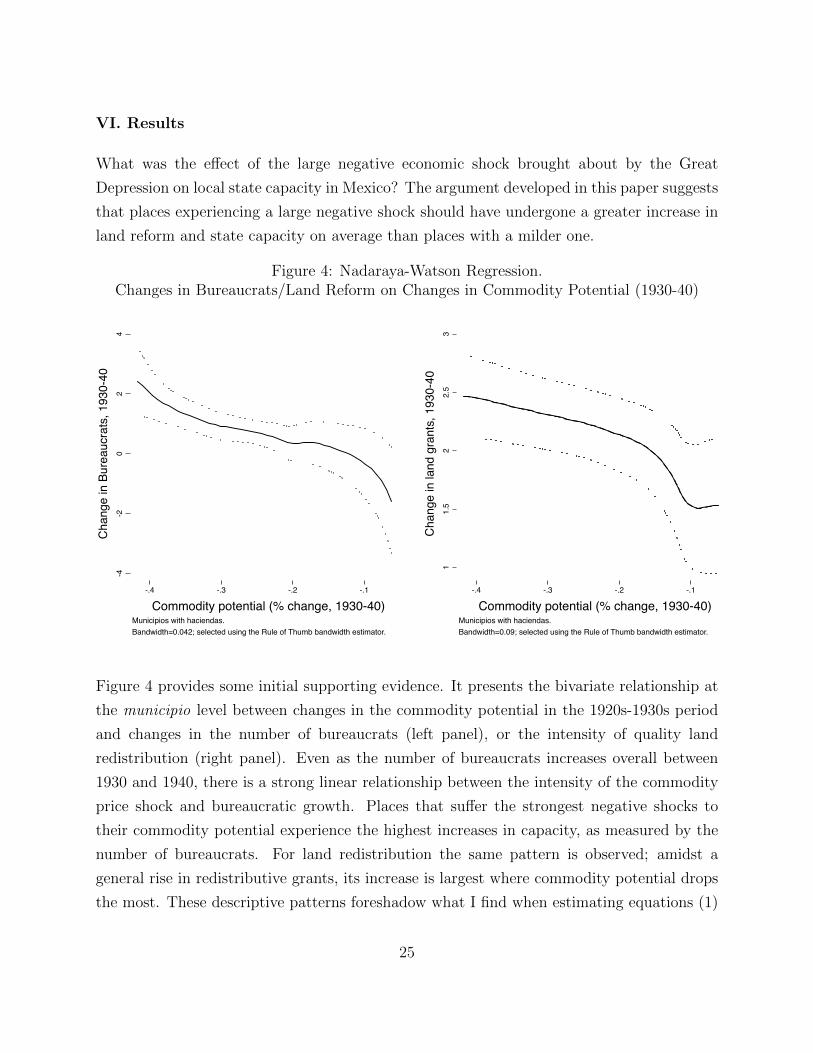
Figure 4: Nadaraya-Watson Regression.Changes in Bureaucrats/Land Reform on Changes in Commodity Potential (1930-40)

-4-2

02

4

Cha

nge

in B

urea

ucra

ts, 1

930-

40

-.4 -.3 -.2 -.1

Commodity potential (% change, 1930-40)Municipios with haciendas. Bandwidth=0.042; selected using the Rule of Thumb bandwidth estimator.

11.

52

2.5

3

Cha

nge

in la

nd g

rant

s, 1

930-

40

-.4 -.3 -.2 -.1

Commodity potential (% change, 1930-40)Municipios with haciendas. Bandwidth=0.09; selected using the Rule of Thumb bandwidth estimator.

Figure 4 provides some initial supporting evidence. It presents the bivariate relationship at

the municipio level between changes in the commodity potential in the 1920s-1930s period

and changes in the number of bureaucrats (left panel), or the intensity of quality land

redistribution (right panel). Even as the number of bureaucrats increases overall between

1930 and 1940, there is a strong linear relationship between the intensity of the commodity

price shock and bureaucratic growth. Places that suffer the strongest negative shocks to

their commodity potential experience the highest increases in capacity, as measured by the

number of bureaucrats. For land redistribution the same pattern is observed; amidst a

general rise in redistributive grants, its increase is largest where commodity potential drops

the most. These descriptive patterns foreshadow what I find when estimating equations (1)

25

and (2).

Table 1: Commodity Shocks and Bureaucrats

(1) (2) (3) (4)Bureaucrats

per 1000 people(Haciendas)

Bureaucratsper 1000 people

(Haciendas)

Bureaucratsper 1000 people(No haciendas)

Bureaucratsper 1000 people

(Haciendas)

Commodity potential (log) -8.10∗ -9.60∗∗ 2.04(4.31) (4.09) (3.19)

Placebocommodity potential (log) -0.36

(0.54)

Population in 1930 (log)× 1940

0.14 1.00∗∗ -0.28

(0.44) (0.45) (0.51)

Municipal surfacearea, Ha. (log) × 1940

0.095 0.14 0.51

(0.29) (0.42) (0.37)

Localities per Ha.in 1930 × 1940

486.2 441.9 428.1

(350.3) (459.0) (347.0)

Population in agriculturein 1930 (%) × 1940

-0.017 -0.012 -0.027

(0.027) (0.022) (0.026)

Population in citiesin 1930 (%) × 1940

-4.26 3.65 -3.47

(3.42) (2.90) (3.37)

Commodity potential (log)in 1930 × 1940 0.0089 0.0046 0.049

(0.17) (0.21) (0.17)

Year FE Yes Yes Yes YesMunicipality FE Yes Yes Yes YesWithin-Municipio Mean of DV 4.28 4.28 2.55 4.28Within-Municipio SD of DV 2.33 2.33 1.77 2.33R sq. 0.73 0.74 0.75 0.73Observations 2904 2904 1434 2904Number of municipios 1506 1506 734 1506

OLS estimations. See equation (1) for the econometric specification. The unit-of-analysis is themunicipio-year. Standard errors (clustered at the municipio level) in parentheses.

Difference-in-differences design. Table 1 shows the difference-in-differences estimates,

equation (1), for the number of bureaucrats per 1000 people.23 The estimated effect of

the commodity potential on state capacity is, as expected, negative, large, and precisely

estimated. Interpreted causally, it suggests a substantial effect: a one standard deviation

decrease in the within-municipio potential induces almost one within-municipio standard

23Alternative measures to those analyzed in tables 1 and 2, the logged number of bureaucrats, andproportion of municipio land redistributed, are presented in table 8 in the appendix, and yield similarresults.

26

deviation increase in the number of bureaucrats per 1000 people. For a municipio at the 25th

percentile of population and state capacity in 1930 (roughly 2,500 people and 2 bureaucrats),

the suggested effect of a negative shock of one within-municipio standard deviation is more

than a two-fold increase in the number of public officials, to 6. In a larger municipio with

average population and state capacity in 1930 (7,700 people with 29 bureaucrats) the effect

of a similarly large shock is an increase of 18 agents of the local government.

These estimated magnitudes are large but plausible, and comparable to the observed changes

in the cases presented above, Chilchota and San Felipe del Progreso. Furthermore, local

expenditure budgets from the state of Chihuahua (available for at least two points in time

for a handful of municipios), support the interpretation that changes in the number of

bureaucrats prioritize order-keeping or extractive activities. For instance, in Balleza, where

the number of local bureaucrats more than doubled from 5 in 1925 to 11 in 1935-38, personnel

in the local treasury increased from one to three tax collectors, in policing from one to two

policemen, and the geographical range of local government was expanded from having no

municipality representative in smaller towns to having three. In Ascencion, where the number

of bureaucrats actually declined from 8 to 7 from 1925 to 1937, a city hall administration

post was re-purposed into a policing position.

Also consistent with the argument, the effect of negative shocks on commodity potential is

only found in places with a landed elite in 1930; places without it have a coefficient that

is orders of magnitude smaller and is not statistically significant (column 3). A placebo

test, reported in column 4, replaces commodity potential with its value one decade into the

future. Any strong association between this placebo and state capacity could indicate the

presence of an underlying differential trend driving the main results. It is reassuring to find

that this is not the case; the coefficient on the placebo commodity potential is small and not

statistically significant.

The mechanism that connects price shocks to investments in state capacity according to

the model is the permanent elimination of the threat posed by the non-ruling economic

elite through the expropriation of their productive asset. In the Mexican context, however,

this did not primarily entail a simple transfer of the asset—here, land—to the new ruling

elite (although this often happened).24 Expropriating land and redistributing it with limited

property rights to peasants allowed incumbent leaders to rely on a non-economic source of

24On occasion, revolutionary generals simply took possession of haciendas for their own profit (e.g.,Wasserman 1993).

27

power in their struggle with the landed elite, and to build a network of political clients with

an entrenched interest in the survival of their patron (Garcıa-Trevino 1953).

Table 2: Commodity Shocks and Land Redistribution

(1) (2) (3) (4)Land reform,

grants(Haciendas)

Land reform,grants

(Haciendas)

Land reform,grants

(No haciendas)

Land reform,grants

(Haciendas)

Commodity potential (log) -3.44∗∗ -5.27∗∗∗ 3.93∗∗∗

(1.69) (1.82) (1.30)

Placebocommodity potential (log) 0.13

(0.33)

Population in 1930 (log)× 1940

2.21∗∗∗ 0.43∗∗ 2.03∗∗∗

(0.38) (0.21) (0.36)

Municipal surfacearea, Ha. (log) × 1940

-0.0090 0.43∗∗∗ 0.14

(0.15) (0.14) (0.16)

Localities per Ha.in 1930 × 1940

45.8 22.3 -0.15

(200.1) (122.8) (186.7)

Population in agriculturein 1930 (%) × 1940

0.021 0.0018 0.017

(0.014) (0.0046) (0.013)

Population in citiesin 1930 (%) × 1940

1.41 0.29 1.79

(1.42) (1.17) (1.43)

Commodity potential (log)in 1930 × 1940 -0.039 0.18∗∗ -0.018

(0.12) (0.083) (0.12)

Land reform by 1930(grants) × 1940 0.25 -0.80∗∗ 0.28

(0.38) (0.33) (0.38)

Year FE Yes Yes Yes YesMunicipality FE Yes Yes Yes YesWithin-Municipio Mean of DV 1.37 1.37 0.35 1.37Within-Municipio SD of DV 1.64 1.64 0.44 1.64R sq. 0.58 0.65 0.61 0.65Observations 3012 3012 1468 3012Number of municipios 1506 1506 734 1506

OLS estimations. See equation (1) for the econometric specification. The unit-of-analysis is themunicipio-year. Standard errors (clustered at the municipio level) in parentheses.

Changes in the municipio-specific commodity potential have the predicted effect on the tra-

jectory of redistributive land grants, as table 2 indicates. The effect is also large, negative,

and statistically significant. A causal interpretation of the coefficient indicates that a one

standard deviation decrease in within-municipio commodity potential leads to one additional

28

land redistribution grant—an increase of almost 80% of a within-municipio standard devia-

tion in the number of redistribution land grants. Again, the effect of shocks is not found in

the placebo specification (when replacing commodity potential with its value ten years into

the future, in column 4).

In places without estates, shocks do have an effect, but in the opposite direction: badly hit

places redistribute less land. The theory presented here cannot account for this finding—it

applies only to cases with a landed elite—but the absence of a similar effect to that estimated

in places with estates helps increase the confidence in the interpretation of the results as

supportive of the theory. In any case, the positive effect of shocks on land redistribution in

the absence of a landed elite is not entirely surprising. A decline in the value of production

would make the petitioning process, a costly affair for landless peasants without a powerful

local sponsor, less attractive. This would lead to a lower likelihood of land redistribution in

places without a landed elite, as the estimates in fact indicate. This finding, then, highlights

the complementarity between the elite-driven account of land reform in Mexico presented

in this paper and demand-driven explanations, in which the dissatisfied and dispossessed

peasants are at the center of land redistributive outcomes (e.g., Saffon 2014; Sellars 2014).

For the case of land grants, I can further assess the main identifying assumption of the

difference-in-differences design—that exposed municipios would maintain the same difference

to unexposed municipios had they not been shocked by the Great Depression. This is

because, unlike data on public officials, redistributive land grants are available for prior

years.25 I find no evidence that prior changes in land grants (between 1920 and 1930) predict

changes in commodity potential, suggesting the plausibility of the identifying assumption

(table 10 in the appendix). Furthermore, when dividing municipios between those most and

least negatively shocked (figure 6 in the appendix), land grants prior to the Great Depression

follow a visibly parallel trend.

Cross-sectional design. So far, the analysis has focused on all types of bureaucrats.26 Does

this pattern also hold when focusing only on local bureaucracy? Estimating the difference-

25Aggregate data on public officials is also available from prior population censuses, but not at themunicipio level.

26During this period, local bureaucrats—state and municipal—were less numerous than federal employees,but concentrated in the least populated areas. This leads to higher levels of local bureaucrats per capitaacross municipios. Furthermore, the federal bureaucracy nominally includes members of the armed forces,which were often controlled by local strongmen, rather than by the central line of command in Mexico City.Taken together, this suggests that the patterns of the bureaucracy can be informative about local statecapacity specifically.

29

in-differences equation (1) for local bureaucrats requires disaggregated data for 1930, which

is not available. For this reason, the cross-sectional empirical approach described in section

IV is implemented using only 1940 data. Table 3 presents the results; they suggest that the

same pattern holds for local bureaucrats.

Table 3: Commodity Shocks and Local Bureaucrats (1940)

(1) (2) (3) (4) (5) (6)Local

bureaucratsper 1000people

Localbureaucrats

per 1000people

Bureaucratsper 1000people

Bureaucratsper 1000people

Landredistribution

(grants)

Landredistribution

(grants)

Commodity potential1920s (log) -0.013 -0.013 0.049 -0.016 0.12 -0.043

(0.016) (0.015) (0.12) (0.093) (0.084) (0.083)

% shock to commoditypotential

-2.08∗∗∗ -1.03∗∗∗ -14.0∗∗∗ -9.77∗∗∗ -4.76∗∗∗ -7.17∗∗∗

(0.35) (0.30) (3.61) (2.78) (1.53) (1.73)

Population, 1930 (log) -0.045 -0.29 2.20∗∗∗

(0.036) (0.28) (0.27)

Bureaucratsper 1000 people,1930

0.017∗∗∗ 0.36∗∗∗

(0.0049) (0.044)

Municipal surfacearea, Ha. (log) 0.13∗∗∗ 0.65∗∗∗ 0.0033

(0.025) (0.20) (0.11)

Localities per Ha., 1930 86.9∗∗ 973.2∗∗ 51.4(37.2) (402.0) (141.9)

Pop. in agriculture1930 (%)

-0.0065∗∗∗ -0.039∗∗∗ 0.021∗∗

(0.0019) (0.014) (0.0098)

Pop. in cities1930 (%)

1.36∗∗∗ 7.72∗∗∗ 1.44

(0.18) (1.49) (1.00)

Land reform by 1930(grants) 2.86∗∗∗ 2.25∗∗∗

(0.31) (0.27)

Mean of DV 0.68 0.69 4.76 4.78 2.63 2.73SD of DV 0.86 0.85 8.02 8.04 6.00 6.13R sq. 0.031 0.24 0.016 0.26 0.18 0.31Number of municipios 1514 1452 1514 1452 1596 1506

OLS estimations. See equation (2) for the econometric specification. The unit-of-analysis is the municipio. Munici-pios with haciendas. Robust standard errors in parentheses.

The first two columns present the estimation of the cross-sectional specification—equation

(2)—using local (municipal) bureaucrats. Using the model with controls, the magnitude

is similar to using all bureaucrats (columns 4 and 5), but smaller than when using the

30

difference-in-differences approach. The mean percentage shock to the commodity potential

from the 1920s to the 1930s is associated with an increase of 13% of the cross-sectional

standard deviation in the number of local bureaucrats per 1000 people. The models for

land reform (models 5 and 6) display the same pattern, with a negative and statistically

significant effect of smaller magnitude than with the difference-in-differences estimation.

Summing up, both empirical strategies—a difference-in-differences approach that compares

places differentially affected by the Great Depression price shocks and a cross-sectional design

in 1940—suggest that negative price shocks generate substantial increases in the expropri-

ation of the productive assets of a non-ruling economic elite (through land reform), and in

state capacity investments (through the number of bureaucrats).

VII. Discussion

The last section presented supportive evidence of the theory’s predictions, and provided

two ways of increasing confidence in the interpretation of the results. First, by assessing

the relationship between commodity shocks and state capacity/land redistribution in the

absence of a landed elite; and second, through a falsification test, using future commodity

shocks. Both strategies provide results supportive of my interpretation. The placebo tests

are estimated to be close to zero and insignificant in all cases, as is the effect of commodity

shocks on state capacity in places without a landed elite.

Yet, a competing interpretation that could be compatible with the results presented thus

far is one in which the federal government directly attempted to create a broader political

coalition that included the peasantry (e.g., Knight 1992). According to this narrative, the

coalition-building promoted by the federal government was underway during this period and

was successful enough to provide stability to the national PRI regime for decades to come.

One implication stemming from this top-down account is that federal land redistribution

efforts should have been focused in places with the highest likelihood of success: those where

landowners were most weakened and thus least able to resist the reform.

When petitioning for land had reached its final stage, at the national level, the president had

the ability to definitively reject petitions. If the president strategically exploited weakened

landed elite to bring peasants into his coalition without incurring high political costs, the

land grant presidential approval rates—conditional on arriving petitions—should have been

higher in the worst-hit regions. Using the difference-in-differences design from equation

(1), however, I find no relationship between shocks and presidential petition approvals; a

31

land petition was as likely to be approved by the president in badly hit regions as it was

in unaffected ones (table 11 in the appendix). That is, I find no evidence linking federal

government actions to the differential commodity shocks after the Great Depression, as

this top-down alternative explanation would have it. These results also rule out a second

alternative interpretation, in which the federal government reacted to the Great Depression

by redistributing land to prevent peasant rebellion (since the worst-hit areas would have

arguably been particularly prone to peasant unrest.)

Given these results, then, what is the long-run significance of this early increase in local state

capacity for the Mexican case? The evidence suggests that the patterns described above—

higher state increases in capacity in places negatively hit by the commodity shock—endure

over the long term.

Table 4 provides suggestive evidence of this persistence. Using the cross-sectional empirical

strategy by estimating equation (2), I find that both available present-day outcomes—the

number of bureaucrats per 1000 people and local tax collection as a proportion of local

GDP—are correlated with the Great Depression price shocks in the expected way. In addition

to estimating models similar to those used for the shorter-term effects, columns 2 and 4

include, for reference, present-day controls (if the estimation were to be interpreted causally,

however, their inclusion could induce post-treatment bias). The magnitude of the effects

relative to variation in state capacity outcomes is comparable to the shorter term effects

presented in the last section (in tables 1 and 3), suggesting that the induced differences

might have set differentially shocked regions on distinct trajectories. Early investments in

capacity were important enough to differentiate the affected from the unaffected municipios

for decades, amidst a process of national convergence in local state capacity.27

One explanation for the observed persistence in capacity can be traced to the process of

political development of the PRI regime. In places where the path to political consolidation

was cleared by the large negative shock brought about by the Great Depression, local political

leaders would have been better able to bargain with the emerging national regime to their

advantage. These local bosses were attractive to the regime because of the control they

exerted in their regions. In exchange for their support to the national ruling coalition,

27Convergence is evidenced by the dispersion in bureaucratic presence, the comparable measure of statecapacity over time. The coefficient of variation for the number of bureaucrats per 1000 people (i.e., standarddeviation divided by the mean) goes from 2.41 in 1930 to 1.8 in 1940 and 0.76 in 2000. The same trend isobserved with the total number of bureaucrats.

32

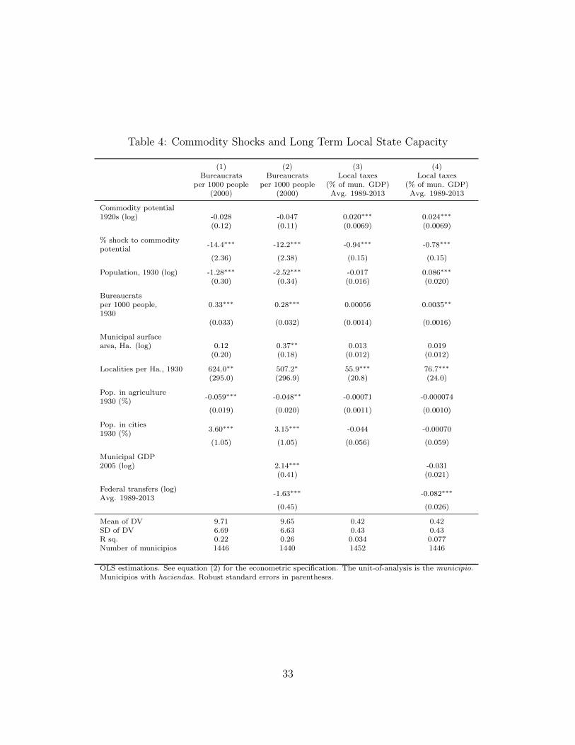
Table 4: Commodity Shocks and Long Term Local State Capacity

(1) (2) (3) (4)Bureaucrats

per 1000 people(2000)

Bureaucratsper 1000 people

(2000)

Local taxes(% of mun. GDP)

Avg. 1989-2013

Local taxes(% of mun. GDP)

Avg. 1989-2013

Commodity potential1920s (log) -0.028 -0.047 0.020∗∗∗ 0.024∗∗∗

(0.12) (0.11) (0.0069) (0.0069)

% shock to commoditypotential

-14.4∗∗∗ -12.2∗∗∗ -0.94∗∗∗ -0.78∗∗∗

(2.36) (2.38) (0.15) (0.15)

Population, 1930 (log) -1.28∗∗∗ -2.52∗∗∗ -0.017 0.086∗∗∗

(0.30) (0.34) (0.016) (0.020)

Bureaucratsper 1000 people,1930

0.33∗∗∗ 0.28∗∗∗ 0.00056 0.0035∗∗

(0.033) (0.032) (0.0014) (0.0016)

Municipal surfacearea, Ha. (log) 0.12 0.37∗∗ 0.013 0.019

(0.20) (0.18) (0.012) (0.012)

Localities per Ha., 1930 624.0∗∗ 507.2∗ 55.9∗∗∗ 76.7∗∗∗

(295.0) (296.9) (20.8) (24.0)

Pop. in agriculture1930 (%)

-0.059∗∗∗ -0.048∗∗ -0.00071 -0.000074

(0.019) (0.020) (0.0011) (0.0010)

Pop. in cities1930 (%)

3.60∗∗∗ 3.15∗∗∗ -0.044 -0.00070

(1.05) (1.05) (0.056) (0.059)

Municipal GDP2005 (log) 2.14∗∗∗ -0.031

(0.41) (0.021)

Federal transfers (log)Avg. 1989-2013

-1.63∗∗∗ -0.082∗∗∗

(0.45) (0.026)

Mean of DV 9.71 9.65 0.42 0.42SD of DV 6.69 6.63 0.43 0.43R sq. 0.22 0.26 0.034 0.077Number of municipios 1446 1440 1452 1446

OLS estimations. See equation (2) for the econometric specification. The unit-of-analysis is the municipio.Municipios with haciendas. Robust standard errors in parentheses.

33

consolidated bosses could have secured local extraction over the long term—using locally

developed capacity—but also increased their ability to place themselves (or their allies) in

high profile national positions.

Table 5: Commodity Shocks and Future National-Level Politicians

(1) (2) (3) (4)Federal government

cabinet members(1940-1970)

Federal governmentcabinet members

(1940-1970)

National-levellegislators

(1940-1970)

National-levellegislators

(1940-1970)

Commodity potential1920s (log) -0.033 -0.041 -0.073 -0.068

(0.038) (0.038) (0.17) (0.16)

% shock to commoditypotential

-2.17∗∗∗ -2.34∗∗ -6.43∗∗ -4.20

(0.82) (1.13) (2.71) (3.46)

Population, 1930 (log) 1.08∗∗∗ 0.77∗∗∗ 4.26∗∗∗ 2.94∗∗∗

(0.19) (0.15) (0.65) (0.58)

Bureaucratsper 1000 people,1930

0.13∗∗∗ 0.31∗∗∗

(0.044) (0.065)

Municipal surfacearea, Ha. (log) -0.32∗∗∗ -0.85∗

(0.11) (0.44)

Localities per Ha., 1930 -142.9 -646.8∗

(95.5) (387.5)

Pop. in agriculture1930 (%)

-0.0072 -0.025∗

(0.0050) (0.014)

Pop. in cities1930 (%)

3.42∗∗∗ 16.0∗∗∗

(0.99) (3.21)

Mean of DV 0.57 0.60 2.52 2.68SD of DV 3.35 3.46 9.85 10.2R sq. 0.099 0.26 0.18 0.36Number of municipios 1557 1452 1557 1452

OLS estimations. See equation (2) for the econometric specification. The unit-of-analysis is the municipio,and the dependent variable measures the total years served by politicians born in each municipio. Municipioswith haciendas. Robust standard errors in parentheses.

To assess the conjecture of consolidation and increased access to national political influence,

I analyze the access to national-level political office associated with each municipio for the

period 1940-1976.28 I construct a geographic political access measure using Roderic Camp’s

28This period spans from immediately after I measure state capacity outcomes following the commodityshocks to the end of president Luis Echeverrıa’s term in 1976. Past analyses of the Mexican nationalpolitical network suggest that a military-based sub-network ruled from the Revolution until Echeverrıa’sterm, replaced later by a finance-based sub-network (Gil-Mendieta and Schmidt 1996). While the miltary-

34

political biographies, and focus on members of Congress and appointed high-ranking officials

(members of the national cabinet, the attorney general, and Justices of the Supreme Court).

After assigning each politician to their place of birth, I add the number of years served in

the Chamber of Deputies and the Senate (or in high-ranking appointments), aggregating to

the municipio level.

Table 5 presents the estimates of the cross-sectional model, equation (2), using the munici-

pio aggregate number of years in national-level political offices as the dependent variable.

Negative shocks following the Great Depression are associated with higher representation

of a municipio in both appointed and elective high-ranking positions (albeit the latter is

less precisely estimated). The results provide evidence for one channel of persistence of the

documented shorter-term effects of temporary landed elite weakness on state capacity. They

also suggest the relevance of political geography as a determinant of the patterns of political

recruitment during the PRI regime, beyond the social characteristics of individual politicians

(e.g., Smith 1979; Camp 1995).

VIII. Conclusion

Large economic shocks that affect elites differentially can disrupt pre-existing political equi-

libria in ways that may be conducive to the development of state capacity. Specifically,

in contexts of intra-elite conflict, shocks may bring about political stability by dispropor-

tionately favoring the incumbent ruler, and opening a window of opportunity during which

this short-lived strength can be consolidated. One such way is the expropriation of assets,

like land, from the temporarily weak elite. By making it advantageous to expropriate a

non-ruling economic elite and extending the time horizon of rulers, these shocks can simul-

taneously induce higher investments in capacity, such as staffing bureaucracies and deploying

public employees, or introducing costly local tax systems.

In this paper, I a presented a simple formalization of these ideas in a two-period, two-agent

model. The key comparative statics that emerge from this model were empirically evalu-

ated with a research design that uses the Great Depression as a shock to post-revolutionary

Mexico. By focusing on local political bosses that emerged from the revolution across the

country, and by using region-specific agro-climatic commodity potential in combination with

based ruling coalition was not characterized by direct intervention of the military in national politics, itscivilian leadership did rely on the support of the military for presidential bids. Furthermore, the military-based sub-network had a regional approach in bringing the country’s economic regions under the regime’scontrol.

35

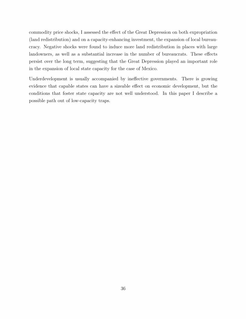
commodity price shocks, I assessed the effect of the Great Depression on both expropriation

(land redistribution) and on a capacity-enhancing investment, the expansion of local bureau-

cracy. Negative shocks were found to induce more land redistribution in places with large

landowners, as well as a substantial increase in the number of bureaucrats. These effects

persist over the long term, suggesting that the Great Depression played an important role

in the expansion of local state capacity for the case of Mexico.

Underdevelopment is usually accompanied by ineffective governments. There is growing

evidence that capable states can have a sizeable effect on economic development, but the

conditions that foster state capacity are not well understood. In this paper I describe a

possible path out of low-capacity traps.

36

References

Acemoglu, Daron, Camilo Garcia-Jimeno and James A. Robinson. 2014. “State Capacity and EconomicDevelopment: A Network Approach.”.

Albertus, Michael. 2011. Political Regimes and Redistribution PhD thesis Stanford University.

Albertus, Michael and Victor Menaldo. 2012. “If You’re Against Them You’re With Us The Effect ofExpropriation on Autocratic Survival.” Comparative Political Studies 45(8):973–1003.

Arias, Luz Marina. 2013. “Building Fiscal Capacity in Colonial Mexico: From Fragmentation to Centraliza-tion.” The Journal of Economic History 73(3).

Bates, Robert and Da-Hsiang Lien. 1985. “A Note on Taxation, Development, and Representative Govern-ment.” Politics & Society 14(1):53–70.

Besley, Timothy and Torsten Persson. 2009. “The Origins of State Capacity: Property Rights, Taxation andPolitics.” The American Economic Review 99(4):1218–1244.

Besley, Timothy and Torsten Persson. 2011. Pillars of Prosperity: Pillars of Prosperity: The PoliticalEconomics of Development Clusters. Princeton University Press.

Bhavnani, Rikhil and Saumitra Jha. 2013. “Forging a Non-Violent Mass Movement: Economic Shocks andOrganizational Innovations in India’s Struggle for Democracy.”.

Brading, David A., ed. 1980. Caudillo and Peasant in the Mexican Revolution. Cambridge University Press.

Calderon, Marco Antonio. 2005. Caciquismo in twen[t]ieth-century Mexico. Institute for the Study of theAmericas chapter Caciquismo and Cardenismo in the Sierra P’urhepecha, Michoacan.

Camp, Roderic Ai. 1995. Political Recruitment across Two Centuries. University of Texas Press.

Camp, Roderic Ai. 2011. Mexican Political Biographies, 1935-2009. University of Texas Press.

Censo de funcionarios y empleados publicos, 1930. 1934. Secretarıa de la Economıa Nacional, Direccion deEstadıstica.

Centeno, Miguel Angel. 2003. Blood and debt: War and the nation-state in Latin America. Penn State Press.

Craig, Ann. 1983. The First Agraristas. University of California Press.

Dell, Melissa. 2012. “Insurgency and Long-Run Development: Lessons from the Mexican Revolution.”.

Dincecco, Mark. 2011. Political Transformations and Public Finances: Europe, 1650–1913. CambridgeUniversity Press.

Dincecco, Mark and Gabriel Katz. 2012. “State Capacity and Long-Run Economic Performance.”.

Evans, Peter. 1995. Embedded autonomy: states and industrial transformation. Princeton University Press.

Fearon, James and David Laitin. 2003. “Ethnicity, insurgency, and civil war.” American Political ScienceReview 97(1):75–90.

Fergusson, Leopoldo, Horacio Larreguy and Juan Felipe Riano. 2015. “Political Competition and StateCapacity: Evidence from a Land Allocation Program in Mexico.” Working Paper .

Fowler-Salamini, Heather. 1978. Agrarian Radicalism in Veracruz, I920-1938. Lincoln.

Gaona, Pedro Hernandez. 1991. “Evolucion y proyeccion de la legislacion agraria mexicana.” Anuario Mex-icano de Historia del Derecho (3):82–94.

37

Garcıa-Trevino, Rodrigo. 1953. “Agrarismo Revolucionario y Ejidalismo Burocratico.” Problemas agrıcolase industriales de Mexico V(4):29–66.

Gil-Mendieta, Jorge and Samuel Schmidt. 1996. “The Political Network in Mexico.” Social Networks18(4):355–381.

Global financial data. 2014.URL: https://www.globalfinancialdata.com/Databases/GFDatabase.html

Haber, Stephen, Noel Maurer and Armando Razo. 2003. The politics of property rights: political instability,credible commitments, and economic growth in Mexico, 1876-1929. Cambridge University Press.

Hamilton, James D. 1992. “Was the Deflation during the Great Depression Anticipated? Evidence from theCommodity Futures Market.” The American Economic Review 82(1):157–178.

Harper, Kristin. 2009. State Governors in the Mexican Revolution, 1910-1952: Portraits in Conflict,Courage, and Corruption. UK: Rowman & Littlefield chapter Tomas Garrido Canabal of Tabasco: RoadBuilding and Revolutionary Reform.

Herbst, Jeffrey. 2000. States and power in Africa: comparative lessons in authority and control. PrincetonUniversity Press.

Knight, Alan. 1992. “Cardenismo: Juggernaut or Jalopy.” Journal of Latin American Studies 26(1):73–107.

Knight, Alan, ed. 2005. Caciquismo in twen[t]ieth-century Mexico. London : Institute for the Study of theAmericas.

Kurtz, Marcus. 2013. Latin American State Building Comparative Perspective. Cambridge University Press.

Lapp, Nancy D. 2004. Landing votes: representation and land reform in Latin America. Palgrave Macmillan.

Levi, Margaret. 1988. Of Rule and Revenue. University of California Press.

Magaloni, Beatriz, Barry Weingast and Alberto Dıaz-Cayeros. 2008. “Why developing countries sabotageeconomic growth: Land reform in Mexico.” Mimeo.

Mann, Michael. 1986. The Sources of Social Power, Volume I. New York: Cambridge University Press.

Mares, Isabela and Didac Queralt. 2015. “The Non-Democratic Origins of Income Taxation.” ComparativePolitical Studies .

Margolies, Barbara. 1975. The Princes of the Earth. Subcutural Diversity in a Mexican Municipality. Amer-ican Anthropoligical Association.

Mayshar, Joram, Omer Moav and Zvika Neeman. 2013. “Geography, Transparency and Institutions.” Work-ing Paper .

Migdal, Joel. 1988. Strong societies and weak states: state-society relations and state capabilities in the ThirdWorld. Princeton University Press.

North, Douglass, John Joseph Wallis and Barry R. Weingast. 2009. Violence and social orders: a conceptualframework for interpreting recorded human history. Cambridge University Press.

Saffon, Maria Paula. 2014. “When Theft becomes Grievance. Dispossessions as a Cause of RedistributiveClaims.” Chapter 2: The Mexican Path.

Sanchez de la Sierra, Raul. 2015. “On the Origin of States: Stationary Bandits and Taxation in EasternCongo.” Working Paper .

Sanderson, Susan Walsh. 1984. Land reform in Mexico, 1910-1980. Florida: Academic Press.

Santoyo, Antonio. 1995. Poder regional y estado en Mexico: Veracruz, 1928-1943. Consejo Nacional para laCultura y las Artes.

38

Scheve, Kenneth and David Stasavage. 2012. “Democracy, war, and wealth: lessons from two centuries ofinheritance taxation.” American Political Science Review 106(1):81–102.

Sellars, Emily. 2014. “Does Emigration Inhibit Political Reform? Evidence from the Mexican AgrarianMovement, 1916-1945.” Working Paper .

Singer, Marion. 1988. El agrarismo en Chiapas (1524-1940). Mexico: INAH.

Skaperdas, Stergios. 1996. “Contest Success Functions.” Economic Theory 7(2):283–290.

Slater, Dan and Hillel Soifer. 2010. “The Indigenous Inheritance: Critical Antecedents and State-Buildingin Latin America and Southeast Asia.”.

Smith, Peter H. 1979. Labyrinths of power: political recruitment in twentieth-century Mexico. PrincetonUniversity Press.

Soifer, Hillel. 2008. “State infrastructural power: Approaches to conceptualization and measurement.”Studies in Comparative International Development 43(3-4):231–251.

Southworth, John R. 1910. The Official Directory of Mines & Estates of Mexico. Mexico, DF: John R.Southworth F.R.G.S.

Thies, Cameron. 2004. “State Building, Interstate and Intrastate Rivalry: A Study of PostColonial Devel-oping Country Extractive Efforts, 1975–2000.” International Studies Quarterly 48(1):53–72.

Thies, Cameron. 2005. “War, rivalry, and state building in Latin America.” American Journal of PoliticalScience 49(3):451–465.

Tilly, Charles. 1992. Coercion, capital, and European states, AD 990-1992. Oxford: Blackwell.

Topalova, Petia. 2010. “Factor Immobility and Regional Impacts of Trade Liberalization: Evidence onPoverty from India.” American Economic Journal: Applied Economics pp. 1–41.

Torres-Mazuera, Gabriela. 2012. La ruralidad urbanizada en el centro de Mexico. UNAM.

Wasserman, Mark. 1993. Persistent Oligarchs. Elites and Politics in Chihuahua, Mexico, 1910-1940. DukeUniversity Press.

39

Appendix

Proof of Proposition 1.

Proof. E’s optimization problem is

max{r}(1− r)p1L+[γ(·)

(p2L+ ω2τ

i2

)+ [1− γ(·)]p2(L− Lj)(1− τ i2)

]).

This payoff is continuous and strictly concave in r ∈ (0, 1), since the contest function γ(·) is strictly

concave in r: ∂∂rγ(·) = Lp1qj

(Lp1r+qj)2> 0, and ∂2

∂r2γ(·) = − 2L2p21q

j

(Lp1r+qj)3< 0. Hence the solution of the

optimization problem will yield a unique interior solution that corresponds to the maximum. Thisis given by the first order condition:

∂

∂ruE(r) = 0,

with uE(r) = (1−r)p1L+[γ(·)

(p2L+ω2τ

i2

)+[1−γ(·)]p2(L−Lj)(1−τ i2)

]. The first order condition

can be written as

p1L =

(Lp1q

j

(Lp1r + qj)2 (p2L+ ω2τi2)− Lp1q

j

(Lp1r + qj)2 [p2(L− Lj)(1− τ i2)]

),

which, after some algebra simplifies to:

r∗ =1

p1L

[√qj(ω2 + p2L)τ i2 + p2Lj(1− τ i2)− qj

].

Note that r is bounded by assumption between [0, 1]. Hence, it takes a value of 0 when√qj(ω2 + p2L)τ i2 + p2Lj(1− τ i2) ≤ qj . I ignore the set of equilibria that arise from this set of

parameter values.

The ruler takes the elites’s best response as given. Recall that, after trivially choosing the maximumlevel of taxation possible and transferring all to himself, R1’s problem becomes

max{j∈{0,1},i∈{0,1}}ω1 + p1Lτ1 − ki +[γ(·)ω2(1− τ i2) + [1− γ(·)][p2Lτ

i2 + ω2]

].

The expropriation condition Γ(j) ≥ 0 guarantees that the decision to expropriate will yield a higherexpected payoff for the local ruler. This follows from the fact that expropriation only affects theprobability of ruler replacement, and period 2 payoffs. It can be written as:

0 ≤ γj=1(·)ω2(1− τ i2) + [1− γj=1(·)][p2Lτi2 + ω2]−

γj=0(·)ω2(1− τ i2) + [1− γj=0(·)][p2Lτi2 + ω2],

which, after some algebra, becomes:

0 ≤ (γj=0(·)− γj=1(·)) (p2L+ ω2).

40

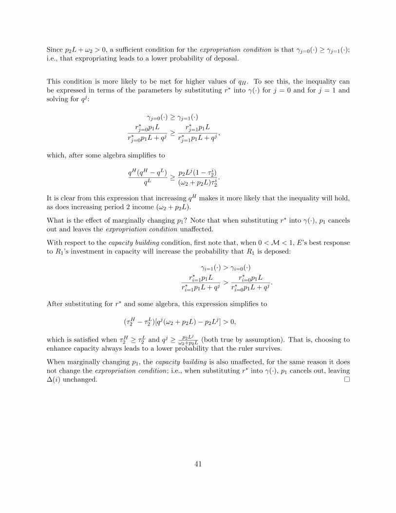
Since p2L+ ω2 > 0, a sufficient condition for the expropriation condition is that γj=0(·) ≥ γj=1(·);i.e., that expropriating leads to a lower probability of deposal.

This condition is more likely to be met for higher values of qH . To see this, the inequality canbe expressed in terms of the parameters by substituting r∗ into γ(·) for j = 0 and for j = 1 andsolving for qj :

γj=0(·) ≥ γj=1(·)r∗j=0p1L

r∗j=0p1L+ qj≥

r∗j=1p1L

r∗j=1p1L+ qj,

which, after some algebra simplifies to

qH(qH − qL)

qL≥ p2L

j(1− τ i2)

(ω2 + p2L)τ i2.

It is clear from this expression that increasing qH makes it more likely that the inequality will hold,as does increasing period 2 income (ω2 + p2L).

What is the effect of marginally changing p1? Note that when substituting r∗ into γ(·), p1 cancelsout and leaves the expropriation condition unaffected.

With respect to the capacity building condition, first note that, when 0 <M < 1, E’s best responseto R1’s investment in capacity will increase the probability that R1 is deposed:

γi=1(·) > γi=0(·)r∗i=1p1L

r∗i=1p1L+ qj>

r∗i=0p1L

r∗i=0p1L+ qj.

After substituting for r∗ and some algebra, this expression simplifies to

(τH2 − τL2 )[qj(ω2 + p2L)− p2Lj ] > 0,

which is satisfied when τH2 ≥ τL2 and qj ≥ p2Lj

ω2+p2L(both true by assumption). That is, choosing to

enhance capacity always leads to a lower probability that the ruler survives.

When marginally changing p1, the capacity building is also unaffected, for the same reason it doesnot change the expropriation condition; i.e., when substituting r∗ into γ(·), p1 cancels out, leaving∆(i) unchanged.

41

Proof of Proposition 2.

Proof. Define p1 ∈ R+ as the value of p1 that solves r∗ when r∗ = 1:

p1 =1

L

[√qj(ω2 + p2L)τ i2 + p2Lj(1− τ i2)− qj

].

For any value of p1 such that p1 ≤ p1, the best E can do is to use all of their available resources toresist R1, by setting r∗ = 1.

As a consequence of this, γj=0(·) = Lp1Lp1r+qL

, and γj=1(·) = Lp1Lp1r+qH

. Since, by assumption qH > qL,

it follows that γj=0(·) > γj=1(·). This leaves the local ruler better off expropriating (j = 1) wheneverp1 ≤ p1.

The investment in capacity decision depends on satifying the capacity building condition (k ≤ ∆(i)):

k ≤{γi=1(·)ω2(1− τH2 )+[1− γi=1(·)][p2Lτ

H2 + ω2]−[

γi=0(·)ω2(1− τL2 ) + [1− γi=0(·)][p2LτL2 + ω2]

]},

which can be simplified to

k ≤{

(τH2 − τL2 )p2L−[p2L+ ω2][γi=1(·)τH2 − γi=0(·)τL2 ]}. (A1)

When p1 ≤ p1, it has been shown that r∗ = 1. E cannot further increase resistance, and thus

γi=0(r∗ = 1) = γi=1(r∗ = 1) = p1Lp1L+qH

. Hence, when p1 ≤ p1, the right hand side of the capacity

building condition reduces to ∆(i, r∗ = 1):

k ≤{

(τH2 − τL2 )[p2L− γ(r∗ = 1)(p2L+ ω2)]}. (A2)

How does equation (A2) compare to (A1)? In other words, when will investments in capacity willhappen for larger values of k? They are larger when p1 ≤ p1 if:{

(τH2 − τL2 )p2L−[p2L+ ω2][γi=1(·)τH2 − γi=0(·)τL2 ]}<{

(τH2 − τL2 )[p2L− γ(r∗ = 1)(p2L+ ω2)]},

which, after some algebra reduces to

τH2 [γi=1(·)− γ(r∗ = 1)] > τL2 [γi=0(·)− γ(r∗ = 1)].

This condition is always true, because τH2 > τL2 and γi=1(·) > γi=0(·).

Given p1 ≤ p1, how does the threshold investment cost, k ≡ ∆(i, r∗ = 1), change with first-periodprices, p1? The partial derivative of k with respect to p1 leads to

−[ LqH

(p1L+ qH)2

](τH2 − τL2 )(p2L+ ω2) < 0.

42

Table 6: Average Spot Prices (USD per metric tonne),Before and After the Great Depression

Commodity 1920-29 1930-39 % ChangeBanana $472.66 $593.60 +25.6%Barley $91.11 $110.00 +20.7%Cacao $1,220.89 $853.86 -30.1%Coffee $1,708.03 $1,135.70 -33.5%Cotton $2,647.34 $1,541.33 -41.8%Maize $35.2 $25.3 -28.2%Rice $591.97 $537.43 -9.2%Sugar $613.42 $489.22 -20.3%Wheat $302.88 $231.50 -23.6%Source: Global Financial Data, from various primary sources.

Table 7: Descriptive Statistics

count mean sd min p25 p50 p75 max

Bureaucratsper 1000 people

4417 3.71 7.21 0 0.81 1.95 3.90 190.1

Number ofbureaucrats (log)

4417 2.21 1.55 0 1.10 2.08 3.14 8.59

Local bureaucratsper 1000 people

2248 0.55 0.82 0 0 0.26 0.82 8.11

Number oflocal bureaucrats, 1940 (log)

2248 1.05 1.16 0 0 0.69 1.79 6.28

Irrigated Land Redistribution(grants)

4417 1.05 3.74 0 0 0 0 93

Irrigated Land Redistribution(% of municipio)

4417 0.0060 0.026 0 0 0 0 0.41

Hacienda in 1930 2169 0.67 0.47 0 0 1 1 1Commodity potential (log) 4417 8.17 1.34 0.48 7.36 8.39 9.08 11.2Placebocommodity potential (log) 4417 8.03 1.43 0.48 7.14 8.21 9.06 11.3Population, 1930 (log) 2169 8.18 1.05 5.21 7.40 8.21 8.91 12.1Pop. in agriculture1930 (%)

2169 30.3 11.8 1.63 25.6 29.0 32.8 204.0

Localities per Ha., 1930 2169 0.00073 0.00083 0.0000044 0.00023 0.00049 0.00096 0.016Municipal surfacearea, Ha. (log) 2169 10.1 1.51 5.46 9.07 10.0 11.1 14.8Pop. in cities1930 (%)

2169 0.057 0.17 0 0 0 0 1

Local taxes (% of mun. GDP)Avg. 1989-2013

2169 0.42 0.48 0 0.16 0.28 0.50 7.55

Bureaucratsper 1000 people(2000)

2140 9.21 7.03 0.22 4.98 7.63 11.2 82.4

Municipal GDP2005 (log) 2169 19.8 1.77 14.9 18.6 19.8 20.9 25.8Federal transfers (log)Avg. 1989-2013

2158 16.6 1.27 13.4 15.8 16.6 17.4 21.3

Federal government cabinetmember-years (1940-1970)

4417 0.25 2.15 0 0 0 0 58

National-levellegislator-years (1940-1970)

4417 1.15 6.24 0 0 0 0 190

43

Table 8: Commodity Shocks, Bureaucrats, and Land RedistributionAlternative Measures

(1) (2) (3) (4) (5) (6)

Bureaucrats(log)

(Haciendas)

Bureaucrats(log)

(Haciendas)

Bureaucrats(log)

(No haciendas)

Landreform

(% of mun.)(Haciendas)

Landreform

(% of mun.)(Haciendas)

Landreform

(% of mun.)(No haciendas)

Commodity potential (log) -0.79∗∗ -1.03∗∗∗ -0.30 0.0082 -0.034∗∗∗ 0.039∗∗

(0.32) (0.36) (0.61) (0.013) (0.010) (0.018)

Population in 1930 (log)× 1940

0.10∗∗ 0.16∗∗ 0.0085∗∗∗ 0.0036

(0.047) (0.076) (0.0021) (0.0023)

Municipal surfacearea, Ha. (log) × 1940

0.0041 -0.031 -0.0047∗∗∗ 0.00021

(0.033) (0.058) (0.0017) (0.0018)

Localities per Ha.in 1930 × 1940

54.6 2.44 6.77 -1.61

(38.4) (86.4) (4.79) (2.26)

Population in agriculturein 1930 (%) × 1940

-0.0028 -0.0013 0.000072 0.000011

(0.0031) (0.0041) (0.00010) (0.000051)

Population in citiesin 1930 (%) × 1940

-0.34∗ 0.41 -0.0044 0.0028

(0.20) (0.33) (0.0075) (0.013)

Commodity potential (log)in 1930 × 1940 -0.0027 -0.044 0.00013 0.0029∗∗∗

(0.024) (0.041) (0.00074) (0.0011)

Land reform by 1930(% of municipio) × 1940 -0.82∗∗∗ -1.01∗∗∗

(0.18) (0.022)

Year FE Yes Yes Yes Yes Yes YesMunicipality FE Yes Yes Yes Yes Yes YesWithin-Municipio Mean of DV 2.61 2.61 1.41 0.0066 0.0066 0.0047Within-Municipio SD of DV 0.57 0.57 0.53 0.0081 0.0081 0.0064R sq. 0.91 0.91 0.88 0.56 0.63 0.71Observations 2904 2904 1434 3012 3012 1468Number of municipios 1506 1506 734 1506 1506 734

OLS estimations. See equation (1) for the econometric specification. The unit-of-analysis is the municipio-year. Standarderrors (clustered at the municipio level) in parentheses.

44

Table 9: Commodity Shocks and Local Bureaucrats (1940)Alternative Measures

(1) (2) (3) (4) (5) (6)Number of

local bureaucrats(log)

Number oflocal bureaucrats

(log)

Number ofbureaucrats

(log)

Number ofbureaucrats

(log)

Landreform

(% of mun.)

Landreform

(% of mun.)

Commodity potential1920s (log) 0.032 -0.022 0.068∗∗ -0.015 0.0014∗∗∗ 0.00011

(0.022) (0.014) (0.028) (0.015) (0.00046) (0.00052)

% shock to commoditypotential

-1.39∗∗∗ -1.06∗∗∗ -1.98∗∗∗ -1.83∗∗∗ 0.015 -0.047∗∗∗

(0.41) (0.30) (0.51) (0.32) (0.010) (0.0099)

Population, 1930 (log) 0.61∗∗∗ 0.87∗∗∗ 0.0084∗∗∗

(0.030) (0.033) (0.0015)

Bureaucratsper 1000 people,1930

0.016∗∗∗ 0.036∗∗∗

(0.0027) (0.0047)

Municipal surfacearea, Ha. (log) 0.12∗∗∗ 0.18∗∗∗ -0.0047∗∗∗

(0.021) (0.025) (0.0012)

Localities per Ha., 1930 88.2∗∗ 172.2∗∗∗ 6.80∗∗

(36.3) (51.1) (3.38)

Pop. in agriculture1930 (%)

-0.0033∗ -0.0020 0.000070

(0.0017) (0.0018) (0.000071)

Pop. in cities1930 (%)

1.57∗∗∗ 1.41∗∗∗ -0.0042

(0.14) (0.14) (0.0053)

Land reform by 1930(% of municipio) 0.28∗ 0.18

(0.15) (0.13)

Mean of DV 1.34 1.36 2.83 2.86 0.011 0.011SD of DV 1.18 1.18 1.48 1.48 0.034 0.033R sq. 0.0085 0.61 0.013 0.72 0.018 0.12Number of municipios 1514 1452 1514 1452 1596 1506

OLS estimations. See equation (2) for the econometric specification. The unit-of-analysis is the municipio. Municipioswith haciendas. Robust standard errors in parentheses.

45

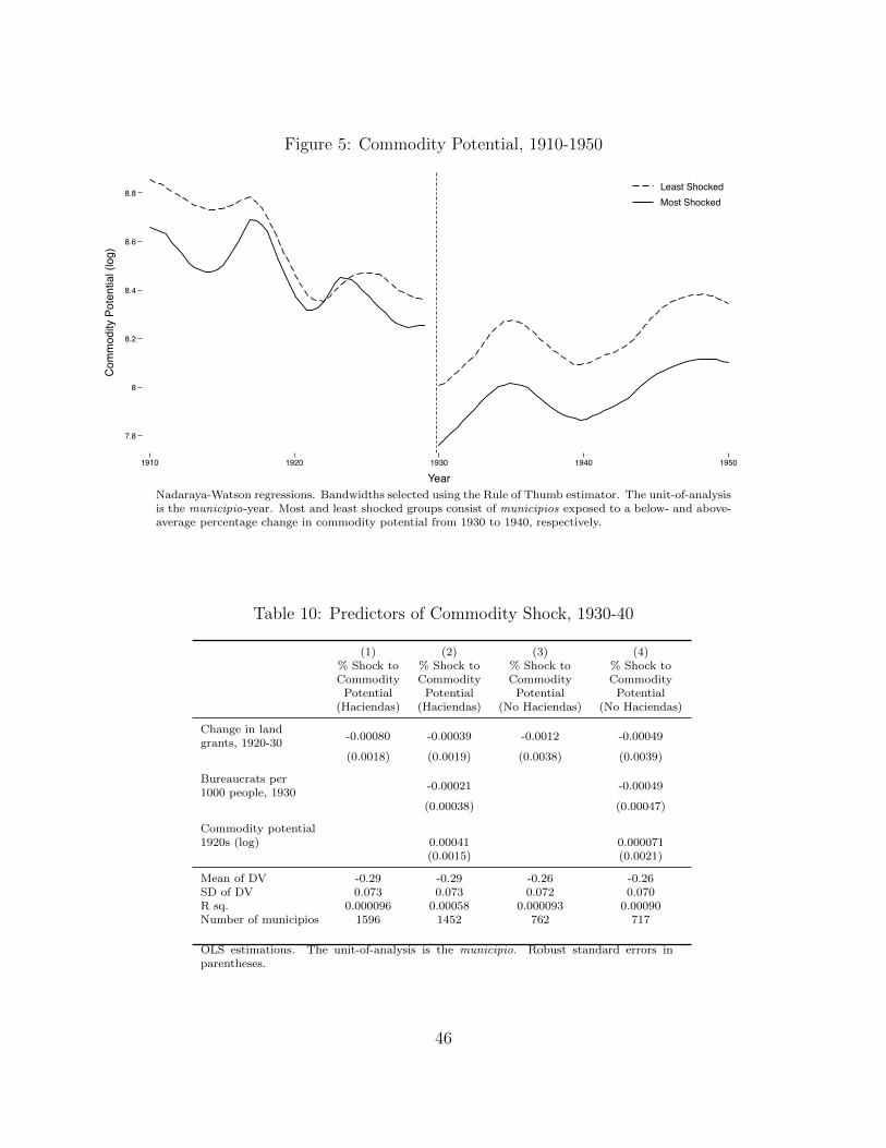
Figure 5: Commodity Potential, 1910-1950

7.8

8

8.2

8.4

8.6

8.8

Com

mod

ity P

oten

tial (

log)

1910 1920 1930 1940 1950

Year

Least ShockedMost Shocked

Nadaraya-Watson regressions. Bandwidths selected using the Rule of Thumb estimator. The unit-of-analysisis the municipio-year. Most and least shocked groups consist of municipios exposed to a below- and above-average percentage change in commodity potential from 1930 to 1940, respectively.

Table 10: Predictors of Commodity Shock, 1930-40

(1) (2) (3) (4)% Shock toCommodity

Potential(Haciendas)

% Shock toCommodity

Potential(Haciendas)

% Shock toCommodity

Potential(No Haciendas)

% Shock toCommodity

Potential(No Haciendas)

Change in landgrants, 1920-30

-0.00080 -0.00039 -0.0012 -0.00049

(0.0018) (0.0019) (0.0038) (0.0039)

Bureaucrats per1000 people, 1930

-0.00021 -0.00049

(0.00038) (0.00047)

Commodity potential1920s (log) 0.00041 0.000071

(0.0015) (0.0021)

Mean of DV -0.29 -0.29 -0.26 -0.26SD of DV 0.073 0.073 0.072 0.070R sq. 0.000096 0.00058 0.000093 0.00090Number of municipios 1596 1452 762 717

OLS estimations. The unit-of-analysis is the municipio. Robust standard errors inparentheses.

46

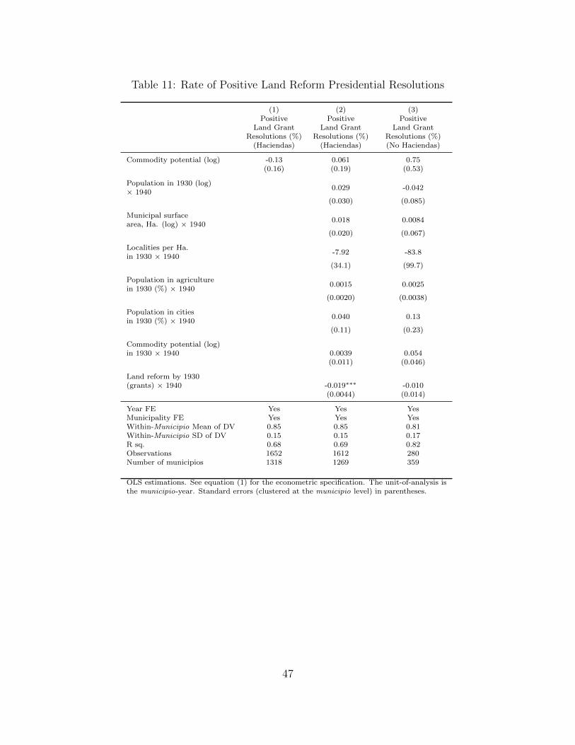
Table 11: Rate of Positive Land Reform Presidential Resolutions

(1) (2) (3)Positive

Land GrantResolutions (%)

(Haciendas)

PositiveLand Grant

Resolutions (%)(Haciendas)

PositiveLand Grant

Resolutions (%)(No Haciendas)

Commodity potential (log) -0.13 0.061 0.75(0.16) (0.19) (0.53)

Population in 1930 (log)× 1940

0.029 -0.042

(0.030) (0.085)

Municipal surfacearea, Ha. (log) × 1940

0.018 0.0084

(0.020) (0.067)

Localities per Ha.in 1930 × 1940

-7.92 -83.8

(34.1) (99.7)

Population in agriculturein 1930 (%) × 1940

0.0015 0.0025

(0.0020) (0.0038)

Population in citiesin 1930 (%) × 1940

0.040 0.13

(0.11) (0.23)

Commodity potential (log)in 1930 × 1940 0.0039 0.054

(0.011) (0.046)

Land reform by 1930(grants) × 1940 -0.019∗∗∗ -0.010

(0.0044) (0.014)

Year FE Yes Yes YesMunicipality FE Yes Yes YesWithin-Municipio Mean of DV 0.85 0.85 0.81Within-Municipio SD of DV 0.15 0.15 0.17R sq. 0.68 0.69 0.82Observations 1652 1612 280Number of municipios 1318 1269 359

OLS estimations. See equation (1) for the econometric specification. The unit-of-analysis isthe municipio-year. Standard errors (clustered at the municipio level) in parentheses.

47

Figure 6: Parallel Trends in Redistributive Land Grants

0

.1

.2

.3

.4

Land

Gra

nts

1920 1925 1930 1935 1940

Year

Most ShockedLeast Shocked

Nadaraya-Watson regressions with 95% confidence intervals. Bandwidths selected using the Rule of Thumbestimator. The unit-of-analysis is the municipio-year. Municipios with haciendas. Most and least shockedgroups consist of municipios exposed to a below- and above-average percentage change in commodity po-tential from 1930 to 1940, respectively.

48