Dr. Y. Aparna, Associate Prof., Dept. of Physics, JNTU College of Engineering, JNTU - H,

Elements of Statistical Mechanics

Question: Discuss about principles of Maxwell-Boltzmann Statistics?

Answer: Maxwell – Boltzmann Statistics

In classical mechanics all the particles (fundamental and composite particles,

atoms, molecules, electrons, etc.). In the system are considered distinguishable. This

means that one can label and track each individual particle in a system. As a consequence

changing the position of any two particles in the system leads to a completely different

configuration of the entire system. Further more there is no restriction on placing more

than one particle in any given state accessible to the system. Classical statistics is called

Maxwell – Boltzmenn Statistics (or M – B Statistics ).

The fundamental future of quantum mechanics that distinguishes it from classical

mechanics is that particles of a particular type or indistinguishable from one another. This

means that in an assemble consisting of similar particles , inter changing any two

particles does not need to a new configuration of the system (in the language of quantum

mechanics; the wave function of the system is invariant with respect to the interchange of

the constituent particles. ). In case of a system consisting of particles belonging to

different nature (for example electrons and protons ), the wave function of the system is

invariant separately for the assembly of the two particles.

While this difference between classical and quantum description of systems is

fundamental to all of quantum statistics, it is further divided in to the following two

classes on the basis of symmetry of the system.

Maxwell – Boltzmann Statistics expression:

Maxwell – Boltzmann statistics describes the statistical distribution of material particles

over various energy states in thermal equilibrium, when the temperature is high enough

and density is low enough to render quantum effects negligible.

The expected number of particles with energy εi for Maxwell – Boltzmann statistics is Ni

Where

Z

kT

Eg

kT

EE

g

N

Ni

i

Fi

ii

−

=

−=

exp

exp

Where: Ni is the number of particles in state i

Ei is the energy of the i-th state

gi is the degeneracy of energy level i, the number of particle’s states

(excluding the free particle state) with energy εi

EF is the chemical potential

K is the Boltzmann’s constant

T is absolute temperature

N is the total number of particles, ∑=i

iNN

Z is the partition function, Z = ∑

−=

i

ii kT

EgZ exp

Equivalently, the distribution is sometimes expressed as

Z

kT

Eg

kT

EEN

Ni

i

Fi

i

−

=

−=

exp

exp

1

Where the index I now specifies a particular state than the set of all states with energy εi.

Question: Explain the principle of Bose-Einstein Statistics?

Answer: Bose – Einstein Statistics

In Bose –Einstein statistics (B- E Statistics ) interchanging any two particles of

the system leaves the resultant system in a symmetric state. That is, the wave function of

the system before interchanging equals the wave function of the system after

interchanging.

It is important to emphasize that the wave function of the system has not changed

itself. This has very important consequences on the state of the system: There is no

restriction to the number of particles that can be placed in a single state (accessible to the

system). It is found that the particles that obey Bose – Einstein statistics are the ones

which have integer spins, which are therefore called bosons (named for Bose). Example

of the bosons include photons and helium – 4 atoms. One type of system obeying B-E

statistics in the Bose – Einstein condensate where all particles of the assembly exist in the

same state.

Question: Discuss about Fermi-Dirac statistics and Fermi-Dirac distribution ?

Answer: Fermi – Dirac statistics

In Fermi – Dirac statistics (F- D statistics) interchanging any two particles of the

system leaves the resultant system in an antisymmetric state. That is, the wavefunction of

the system before interchanging is the wavefunction of the system after interchanging,

with an overall minus sign

Again it should be noted that the wavefunction of the system itself does not

change. The consequence of the negative sign on the Fermi – Dirac statistics can be

understood in the following way:

Suppose that the particles that are interchanged belong to the same state. Since the

particles are considered indistinguishable from one another then changing the coordinates

of the particles should not have any change on the system’s wavefunction (because by

our assumption the particles are in the same state). Therefore, the wavefunction before

interchanging similar states equals the wavefunction after interchanging similar states.

Combining (or adding, literally speaking) the above statement with the

fundamental symmetry of the Fermi –Dirac system leads us to conclude that the

wavefunction of the system before interchanging equals zero.

This shows that in Fermi –Dirac statistics, more than one particle cannot occupy a

single state accessible to the system. This is called pauli’s exclusion principle.

It is found that particles with half – integral spin (or fermions) obey the Fermi –

Dirac statistics. This includes, electrons, protons, Helium – 3 etc.

Fermi – Dirac and Bose – Einstein statistics apply when quantum effects are

important and the particles are indistinguishable. Quantum effects appear if the

concentration of particles (N/V) ≥ nq. here nq is the quantum concentration, for which

the interparticle distance is equal to the thermal de Broglie wavelength, so that the

wavefunctions of the particles are touching but not overlapping. Fermi- Dirac statistics

apply to fermions (particles that obey the pauli exclusion principle), and Bose – Einstein

statistics apply to bosons. As the quantum concentration depends on temperature; most

systems at high temperatures obey the classical (Maxwell – Boltzmann ) limit unless they

have a very high density, as for a white dwarf. Both Fermi – Dirac and Bose- Einstein

become Maxwell – Boltzmann statistics at high temperature or at low concentration.

Maxwell – Boltzmann statistics are often described as the statistics of

distinguishable classical particles. In other words the configuration of particle A in state

1 and particle B in state 2 is different from the case where particle B is in state 1 and

particle A is in state 2. This assumption leads to the proper (Boltzmann) distribution of

particles in the energy states, but yields non – physical results for the entropy, as

embodied in the Gibbs paradox. This problem disappears when it is realized that all

particles are in fact indistinguishable. Both of these distributions approach the Maxwell –

Boltzmann distribution in the limit of high temperature and low density, with out the

need for any ad hoc assumptions. Maxwell – Boltzmann statistics are particularly useful

for studying gases. Fermi – Dirac statistics are most often used for the study of electrons

in solids. As such, they form the basic of semiconductor device theory and electrons.

Fermi – Dirac distribution:

For a system of identical fermions, the average number of fermions in a single – particle

state i, is given by the Fermi –Dirac (F-D) distribution.

1exp

1

+

−=

kT

EEn

Fii

Where K is Boltzmann’s constant, T is the absolute temperature, Ei is the energy of

the single – particle state I, and EF is the chemical potential. For the case of electrons

in a semiconductor, EF is also called the Fermi level.

The F-D distribution is valid only if the number of fermions in the system is large

enough so that adding ine more fermion to the system has negligible effect on EF.

since the F-D distribution was delivered using the Pauli exclusion principle, a result

is that 0<ni<1.

Question: Discuss about the properties of Fermi-Dirac Statistics ?

Answer: Properties of the Fermi – Dirac statistics

In a semiconductor, the probability of occupancy of states by electrons is given by

the Fermi – Dirac distribution function.

=== FDe PFPEF )()(

−+

kT

EE Fexp1

1

(8.1)

i. The distribution function Pe (E) is valid only in equilibrium.

ii. EF is denotes an energy level and is called fermi energy level. It is strictly

valid in equilibrium.

iii. It is applicable for all insulators, semiconductors and metals.

iv. It considers all electrons in semiconductors and not merely electrons in a

band.

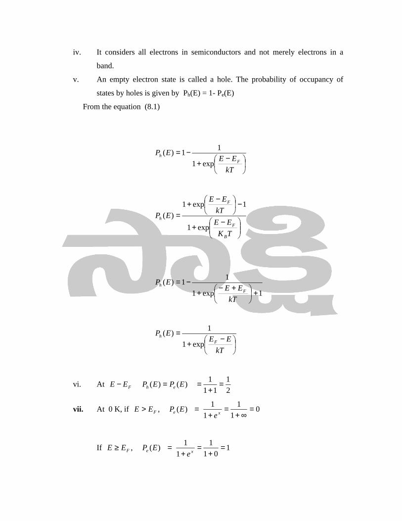
v. An empty electron state is called a hole. The probability of occupancy of

states by holes is given by Ph(E) = 1- Pe(E)

From the equation (8.1)

−+

−=

kT

EEEP

Fh

exp1

11)(

−+

−

−+

=

TK

EE

kT

EE

EP

B

F

F

h

exp1

1exp1

)(

1exp1

11)(

+

+−+

−=

kT

EEEP

Fh

−+

=

kT

EEEP

Fh

exp1

1)(

vi. At 2

1

11

1)()( =

+==− EPEPEE ehF

vii. At 0 K, if 01

1

1

1)(, =

∞+=

+=>

xeFe

EPEE

If 101

1

1

1)(, =

+=

+=≥

xeF eEPEE

This means that at absolute zero temperature, energy states up to the Fermi level

are completely occupied by electrons, and the levels above EF are empty i.e.

For all,

==

<<

−>>−

1)(

0)(,1exp,

EP

EPhence

kT

EEkTEE

h

eTF

For all,

==

<<

−>>−

0)(

1)(,1exp,

EP

EPhence

kT

EEkTEE

h

eTF

viii. the functions Pe(E) and Ph(E) possess a certain symmetry about the Fermi

level as shown in Fig. 8.1. consider a level (Ep +δ E) just above the Fermi

level. The electron occupancy at this level is

fig 1: Fermi –Dirac distribution of electrons

+−+=+

kT

EEEEEP

FFFe δ

δexp1

1)(

+=+

kT

EEEP Fe δ

δexp1

1)(

Similarly the hole occupancy at a level EF - δ E just below the Fermi level is

+−+=−

kT

EEEEEP

FFFh δ

δexp1

1)(

+=−

kT

EEEP Fh δ

δexp1

1)(

Hence,

=+ )( EEP Fe δ )( EEP Fh δ−

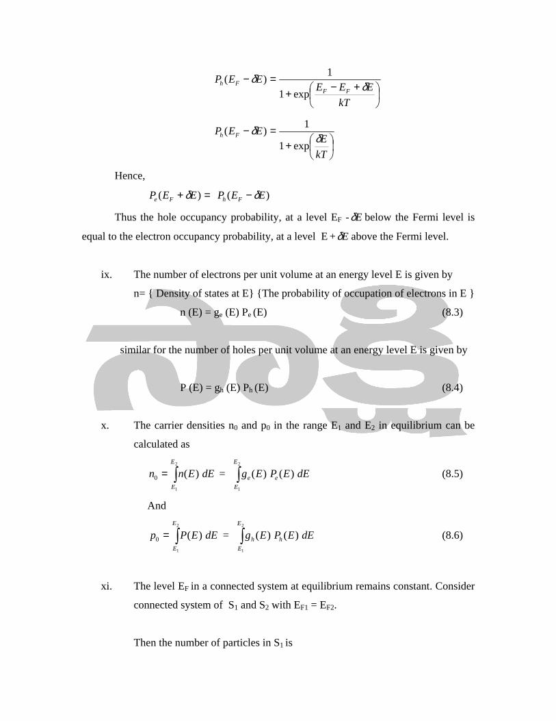
Thus the hole occupancy probability, at a level EF - Eδ below the Fermi level is

equal to the electron occupancy probability, at a level E + Eδ above the Fermi level.

ix. The number of electrons per unit volume at an energy level E is given by

n= { Density of states at E} {The probability of occupation of electrons in E }

n (E) = ge (E) Pe (E) (8.3)

similar for the number of holes per unit volume at an energy level E is given by

P (E) = gh (E) Ph (E) (8.4)

x. The carrier densities n0 and p0 in the range E1 and E2 in equilibrium can be

calculated as

∫=2

1

)(0

E

E

dEEnn = ∫2

1

)()(E

E

ee dEEPEg (8.5)

And

∫=2

1

)(0

E

E

dEEPp = ∫2

1

)()(E

E

hh dEEPEg (8.6)

xi. The level EF in a connected system at equilibrium remains constant. Consider

connected system of S1 and S2 with EF1 = EF2.

Then the number of particles in S1 is

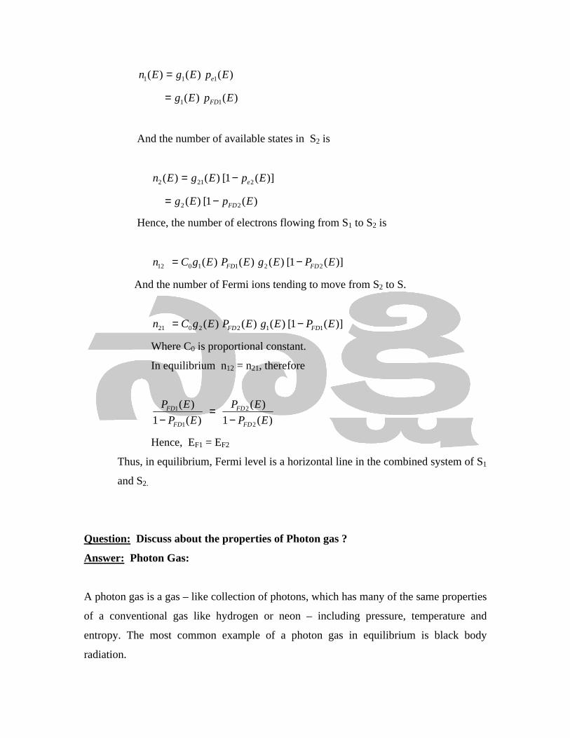
)()()( 111 EpEgEn e=

)()( 11 EpEg FD=

And the number of available states in S2 is

)](1[)()( 2212 EpEgEn e−=

)(1[)( 22 EpEg FD−=

Hence, the number of electrons flowing from S1 to S2 is

)](1[)()()( 2211012 EPEgEPEgCn FDFD −=

And the number of Fermi ions tending to move from S2 to S.

)](1[)()()( 1122021 EPEgEPEgCn FDFD −=

Where C0 is proportional constant.

In equilibrium n12 = n21, therefore

=− )(1

)(

1

1

EP

EP

FD

FD

)(1

)(

2

2

EP

EP

FD

FD

−

Hence, EF1 = EF2

Thus, in equilibrium, Fermi level is a horizontal line in the combined system of S1

and S2.

Question: Discuss about the properties of Photon gas ?

Answer: Photon Gas:

A photon gas is a gas – like collection of photons, which has many of the same properties

of a conventional gas like hydrogen or neon – including pressure, temperature and

entropy. The most common example of a photon gas in equilibrium is black body

radiation.

A massive ideal gas with only one type of particle is uniquely described by three state

functions such as the temperature, volume and the number of particles. However for a

black body, the energy distribution is established by the interaction of the photons with

matter, usually the walls of the container. In this interaction the number of photons is not

conserved. As a result the chemical potential of the black body photon gas is zero. The

number of state functions needed to describe a black body state thus reduced from three

to two (e.g. temperature and volume).

In a gas with massive particles, the energy of the particles is distributed according

to a Maxwell – Boltzmann distribution. This distribution is established as the particles

collide with each other, enhancing energy (and momentum) in the process. In a photon

gas, there will also be an equilibrium distribution, but photons do not collide with each

other (except under very extreme conditions) so that the equilibrium distribution must be

established by her means. The most common way than an equilibrium distribution is

established is by the interaction of the photons with matter. If the photons are absorbed

and emitted by the walls of the system containing the photon gas, and the walls are at a

particular temperature, when the equilibrium distribution for the photons will be back

body distribution at that temperature.

A very important difference between a gas of massive particles and a photon gas

with black body distribution is that the number of photons in the system is not conserved.

A photon may collide with an electron in the wall, exciting it to a higher energy state,

removing a photon from the photon gas. The electron may drop back to its lower level

a serious of steps, each one of which releases an individual photon back into the photon

gas. Although the sum of the energies of the emitted photons are the same as the

absorbed photon, the number of emitted photons will vary. It can be shown that, as a

result of this back of constraint on the number of photons in the system, the chemical

potential of the photons must be zero for blackbody radiation.

The thermodynamics of a black body photon gas may be derived using quantum technical

arguments. The derivation yields the spectral energy distribution u which is the energy

per unit volume per unit frequency interval:

1exp

18),(

3

3

−

=

kT

hvc

hvTvu

π

Where h is Planck’s constant, c is the speed of light, ν is the frequency, k is the

Boltzmann’s constant, and T is temperature.

Question: What is Wein’s displacement law?

Answer: Wien’s Displacement Law:

Wien’s displacement law states that the black body curve at any temperature is

uniquely determined from the block body curve at any temperature is uniquely

determined from the black body curve at any other temperature by displacing, or

shifting, the wavelength. The average thermal energy/ frequency in each mode with

frequency v is only a function of v/T. Restarted in terms of the wavelength vc=λ ,

the distribution at corresponding wavelengths are related, where corresponding

wavelengths are at locations proportional to 1/T.

From this law, it follows that there is an inverse relationship between the

wavelength of the peak of the emission of a black body and its temperature, and this

less powerful consequence is often also called Wien’s displacement law is

T

b=maxλ

Where

maxλ is the peak wavelength in meters

T is the temperature of the black body in kelvins (K), and

b is a constant of proportionality, called Wien’s displacement constant.

Question: What is Rayliegh – Jeans law?

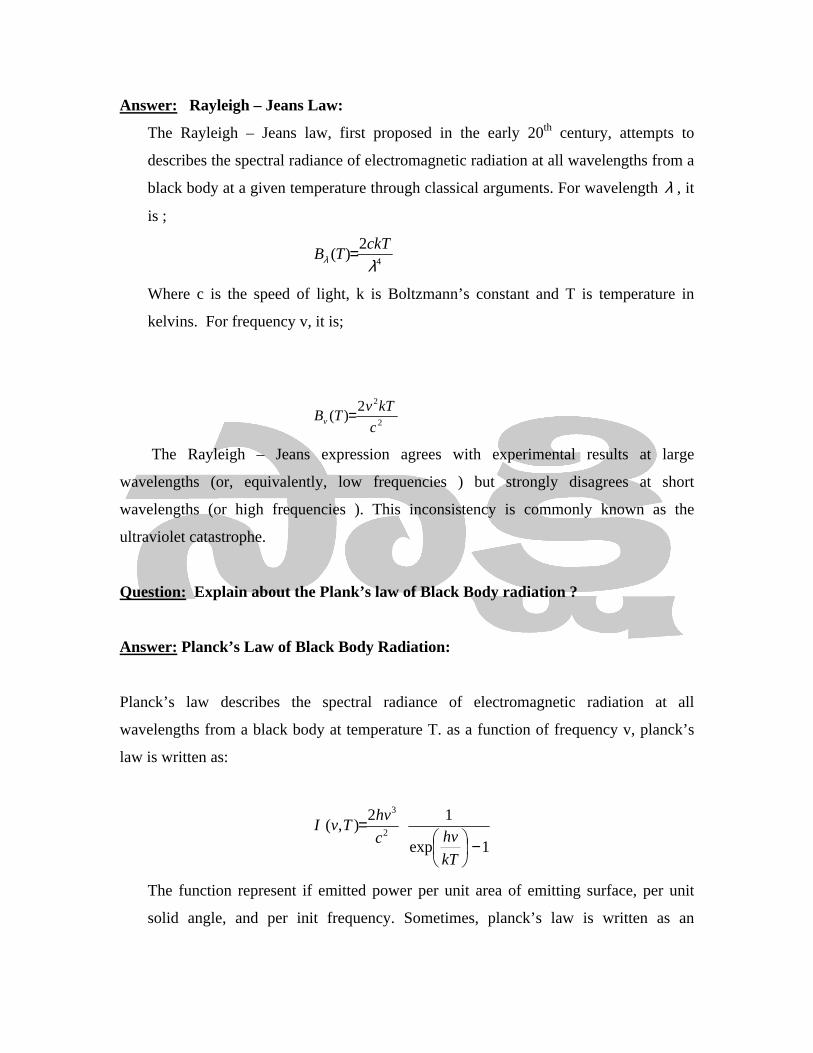
Answer: Rayleigh – Jeans Law:

The Rayleigh – Jeans law, first proposed in the early 20th century, attempts to

describes the spectral radiance of electromagnetic radiation at all wavelengths from a

black body at a given temperature through classical arguments. For wavelength λ , it

is ;

4

2)(

λλckT

TB =

Where c is the speed of light, k is Boltzmann’s constant and T is temperature in

kelvins. For frequency v, it is;

2

22)(

c

kTvTBv =

The Rayleigh – Jeans expression agrees with experimental results at large

wavelengths (or, equivalently, low frequencies ) but strongly disagrees at short

wavelengths (or high frequencies ). This inconsistency is commonly known as the

ultraviolet catastrophe.

Question: Explain about the Plank’s law of Black Body radiation ?

Answer: Planck’s Law of Black Body Radiation:

Planck’s law describes the spectral radiance of electromagnetic radiation at all

wavelengths from a black body at temperature T. as a function of frequency v, planck’s

law is written as:

1exp

12),(

2

3

−

=

kT

hvc

hvTvI

The function represent if emitted power per unit area of emitting surface, per unit

solid angle, and per init frequency. Sometimes, planck’s law is written as an

expression ),(),( TvITvu π= for emitted power integrated over all solid angles. In

other cases, it is written as cTvITvu /),(4),( π= for energy per unit volume.

The function I(v, T) peaks for hv= 2.82 kT. It falls off exponentially at higher

frequencies and polynomially at lower. As a function of wavelength λ , plank’s law

written (for unit solid angle ) as:

1exp

12),('

5

2

−

=

kT

hchc

TI

λλ

λ

This function peaks for hc = 4.97 kTλ , a factor of 1.76 shorter in wavelength

(higher in frequency ) then the frequency peak. It is the more commonly used peak in

Wien’s displacement law.

The radiance emitted over a frequency range [v1, v2] or a wavelength range

[ ] [ ]1212 /,/, vcvc=λλ can be obtained by integrating the representing the respective

functions.

∫ ∫=2

1

1

2

),('),(v

v

dTIdvTvIπ

λ

λλ

The order of the integration limits is reversed because increasing frequencies

correspond to decreasing wavelengths.

The wavelength is related to the frequency by:

v

c=λ

The is some times written in terms of spectral energy density.

1exp

18),(

4),(

3

3

−

==

kT

hvc

hvTvI

cTvu

ππ

Which has units of energy per unit volume per unit frequency (joule per cubic meter

per hertz). Integrated over frequency, this expression yields the total energy density,

the radiation field of a black body may be thought of as a photon gas, in which case

this energy density would be one of the thermodynamic parameters of that gas.

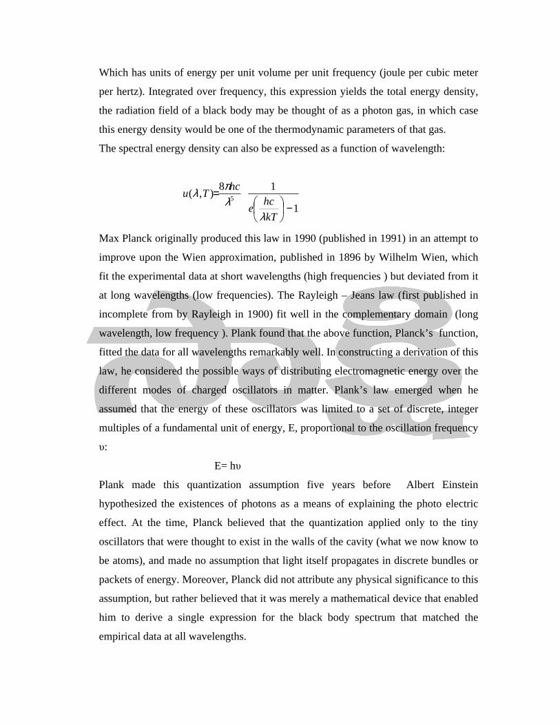
The spectral energy density can also be expressed as a function of wavelength:

1

18),(

5

−

=

kT

hce

hcTu

λλπλ

Max Planck originally produced this law in 1990 (published in 1991) in an attempt to

improve upon the Wien approximation, published in 1896 by Wilhelm Wien, which

fit the experimental data at short wavelengths (high frequencies ) but deviated from it

at long wavelengths (low frequencies). The Rayleigh – Jeans law (first published in

incomplete from by Rayleigh in 1900) fit well in the complementary domain (long

wavelength, low frequency ). Plank found that the above function, Planck’s function,

fitted the data for all wavelengths remarkably well. In constructing a derivation of this

law, he considered the possible ways of distributing electromagnetic energy over the

different modes of charged oscillators in matter. Plank’s law emerged when he

assumed that the energy of these oscillators was limited to a set of discrete, integer

multiples of a fundamental unit of energy, E, proportional to the oscillation frequency

υ:

E= hυ

Plank made this quantization assumption five years before Albert Einstein

hypothesized the existences of photons as a means of explaining the photo electric

effect. At the time, Planck believed that the quantization applied only to the tiny

oscillators that were thought to exist in the walls of the cavity (what we now know to

be atoms), and made no assumption that light itself propagates in discrete bundles or

packets of energy. Moreover, Planck did not attribute any physical significance to this

assumption, but rather believed that it was merely a mathematical device that enabled

him to derive a single expression for the black body spectrum that matched the

empirical data at all wavelengths.

Although Planck’s formula predicts that a black body will radiate energy at all

frequencies, the formula is only practically applicable when many photons are being

measured. For example, a black body at room temperature (300 kelvin ) with one

square meter or surface area will emit a photon in the visible range once about every

thousand years or so, meaning that for most practical purpose, a black body at room

temperature does not emit in the visible range. Significance of this fact for the

derivation of Planck’s law from experiment data, and for the substantiation of the law

by the data is discussed.

Ultimately, Planck’s assumption of energy quantization and Einstein’s photon

hypothesis became the fundamental basis for the development of quantum mechanics.

Question: What is concept of free electron gas?

Answer: Concept of Electron Gas and exaplain about root mean square (rms)

velocity:

In 1990, Drude and Lorentz proposed the classical free electron theory. According to

this theory, metal is an aggregate of fixed positive charges and negative free electron

gas and the free electron gas is obeying the laws of Kinetic theory of gases. This

means electrons can be assigned a mean free path, a mean collision time and average

speed. The silent features of classical free electron theory are given below.

i. The free electrons, in all metals behave as the molecules of a gas in a

container.

ii. The mutual repulsion among the electrons is ignored, so that they move in all

the directions with all the possible velocities.

iii. As the electrons move randomly with rms velocity, the resultant velocity of

them in a particular direction will be zero.

iv. If the potential difference is created across the metal then free electrons

slowly drift towards the positive potential or in the opposite direction to the

applied electric field even though they collide continually with one another

and fixed positive metal ions in the lattice. The acquired velocity by the

electrons is called drift velocity and is represented by vd.

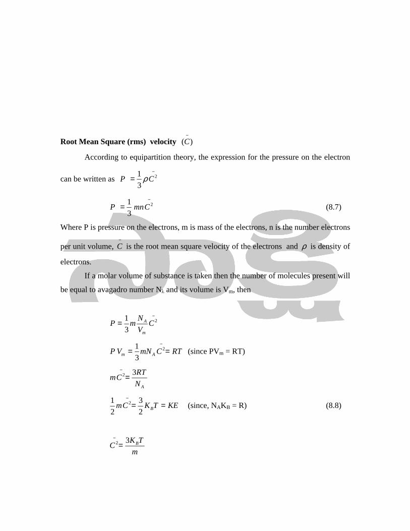
Root Mean Square (rms) velocity )(−C

According to equipartition theory, the expression for the pressure on the electron

can be written as −

= 2

3

1CP ρ

−

= 2

3

1CmnP (8.7)

Where P is pressure on the electrons, m is mass of the electrons, n is the number electrons

per unit volume, −C is the root mean square velocity of the electrons and ρ is density of

electrons.

If a molar volume of substance is taken then the number of molecules present will

be equal to avagadro number Nλ and its volume is Vm, then

−

= 2

3

1C

V

NmP

m

A

RTCmNVP Am ==−

2

3

1 (since PVm = RT)

AN

RTCm

32=−

KETKCm B ==−

2

3

2

1 2 (since, NAKB = R) (8.8)

m

TKC B32=

−

m

TKC B3=−

(8.9)

31

23

101.9

3001038.13−

−−

××××=C

smC /1016.1 5×=−

Hence, the free electron gas is moving with smC /1016.1 5×=−

velocity. Thus it is in

motion, the resultant displacement will be zero as it is in random motion and no currents

are present in the metal when there are no external forces.

Question: Explain Fermi level and Fermi energy with the help of suitable

diagram?

Answer: Fermi Energy:

The Fermi energy is a concept in quantum mechanics usually referring to the energy of

the highest occupied quantum state in a system of fermions at absolute zero temperature.

This article requires a basic knowledge of quantum mechanics.

Note that the term Fermi energy is often, confusingly, used to describe a different but

closely related concept, the Fermi level (also called chemical potential ). The Fermi

energy and chemical potential are the same at absolute zero, but differ at other

temperatures, as described below.

In quantum mechanics, a group of particles known as fermions (for example, electrons,

photons and neutrons are fermions ) obey the Pauli exclusion principle, which states that

no two fermions can occupy the same quantum state. The states are lebeled by a set of

quantum numbers. In a system containing many fermions (like electrons in a metal) each

fermion will have a different set of quantum numbers. To determine the lowest energy

system of fermions can have, we first group the states into sets with equal energy, and

order these sets by increasing energy. Starting with an empty system, we then add

particles one at a time, consecutively filling up the unoccupied quantum states with the

lowest energy. When all the particles have been put in, the Fermi energy is the energy is

the energy of the highest occupied state. What this means is that even if we have

extracted all possible energy from a metal by cooling it down to near absolute zero

temperature (0 kelvins), the electrons in the metal are still moving around; the fastest

ones would be moving at a velocity that corresponds to a kinetic energy equal to the

Fermi energy. This is the Fermi velocity. The Fermi energy is one of the important

concepts of condensed matter physics. It is used, for example, to describe metals,

insulators and semiconductors. It is a very important quantity in the physics of

superconductors, in the physics of quantum liquids like low temperature helium (both

normal and superfluid 3He), and it is quite important to nuclear physics and to

understand the stability of white dwarf starts against gravitational collapse.

The Fermi energy (EF) of a system of non – interacting fermions is the increase in the

ground state energy when exactly one particle is added to the system. It can also be

interpreted as the maximum energy of an individual fermion in this ground state. The

chemical potential at zero temperature is equal to the Fermi energy.

The probability to find an electron in an energy state of energy E can be expressed as

−+=

kT

EEEF

Fexp1

1)( (8.10)

Where F(E) is called the Fermi Dirac distribution function. E is the energy level

occupied by the electron and EF is the Fermi level and is constant for a particular

system.

The Fermi level is a boundary energy level which separates the filled energy

states and empty energy states at 0 K. The energy of the highest filled state at 0 K is

called the Fermi energy level is known as Fermi level. It is shown in Fig. 8.2.

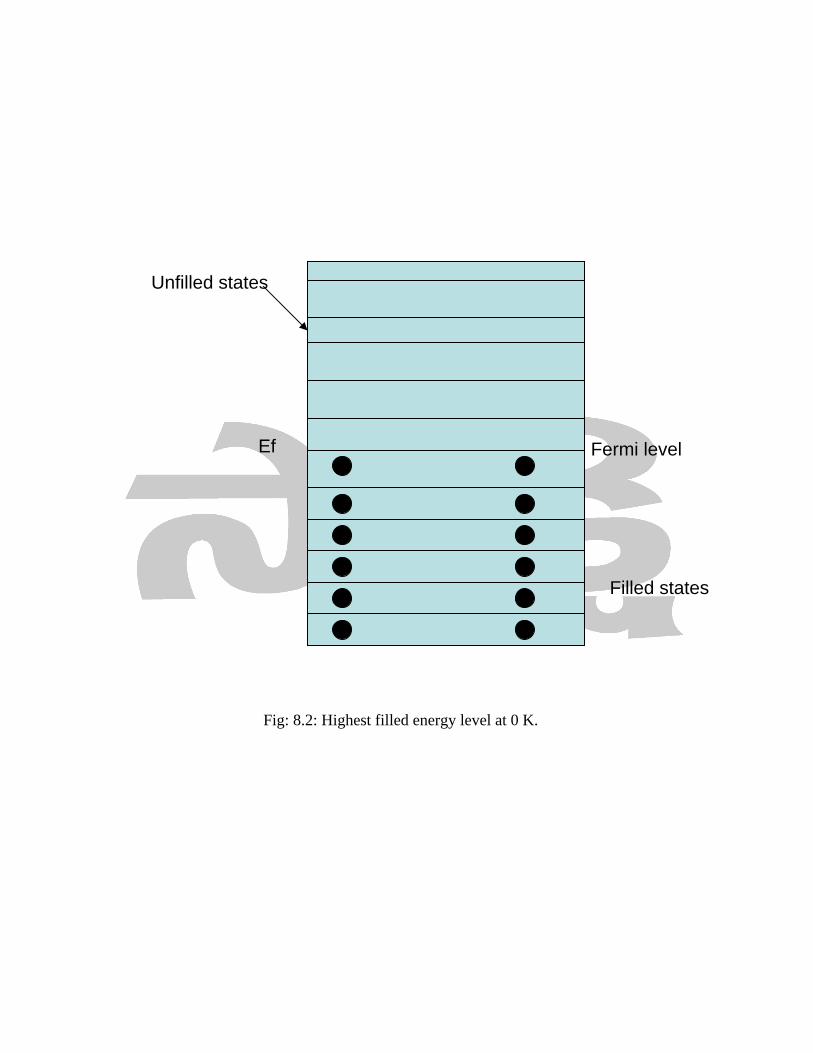
Fig: 8.2: Highest filled energy level at 0 K.

Fermi level Ef

Unfilled states

Filled states

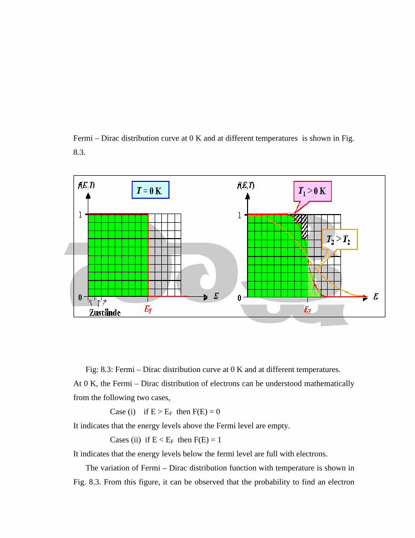
Fermi – Dirac distribution curve at 0 K and at different temperatures is shown in Fig.

8.3.

Fig: 8.3: Fermi – Dirac distribution curve at 0 K and at different temperatures.

At 0 K, the Fermi – Dirac distribution of electrons can be understood mathematically

from the following two cases,

Case (i) if E > EF then F(E) = 0

It indicates that the energy levels above the Fermi level are empty.

Cases (ii) if E < EF then F(E) = 1

It indicates that the energy levels below the fermi level are full with electrons.

The variation of Fermi – Dirac distribution function with temperature is shown in

Fig. 8.3. From this figure, it can be observed that the probability to find an electron

decreases below the Fermi level and increases above the Fermi level as temperature

increase. And there exists a two – fold symmetry un the probability curves about the

Fermi level.

The product of Fermi – Dirac distribution function and density of states gives the

number of electrons per unit volume

i.e., ∫=FE

dEEgEFn0

)()( (8.11)

substituting F(E) and G(E) values in equation 8.11

∫

−+=

FE

F

dEEh

m

kT

EEn

0

2

12

3

2

8

2exp1

1 π

If a metal is taken at 0 K then energy levels below Fermi level are filled by electrons

and above Fermi level are empty. If T = 0 K and E<EF , then

∫

=FE

dEEh

mn

0

2

12

3

2

8

2

π

∫

=FE

dEEh

mn

0

2

12

3

2

8

2

π

FE

E

h

mn

0

2

3

2

3

2

2

38

2

= π

3

223

2

8

3n

m

hEF

=π

3

2

2

23

2

8

3n

m

hEF

=π

Substituting the values of h, n, m and π , the Fermi energy,

EF = 3.62 x 10 19 n 23 eV

Question: Give a short notes on Density of states in an atom?

Answer: Density of States:

The number of electrons present per unit volume in an energy level at a given

temperature is equal to the product of density of states (number of energy levels per unit

volume) and Fermi – Dirac distribution function (the probability to find an electron).

Therefore, to calculate the number of electrons in an energy level at a given temperature,

it is must to know the number of energy states per unit volume.

The number of energy states with a particular energy value E is depending on how many

combinations of the quantum numbers resulting in the same value n. the energy levels

appear continuum inside the space of an atom, therefore, let nx, ny, and nz (n2 = nx

2 + ny2 +

nz2) in the three dimensional space. In this space every integer specifies an energy level

i.e., each unit cube contains exactly one state. Hence the number of energy states in any

volume in units of cubes of lattice parameters.

Consider a space of radius n and another sphere of radius (n + dn) in which energy values

are E and E + dE respectively as shown in Fig. 8.4. hence, the number of energy states

available in the sphere of radius n is

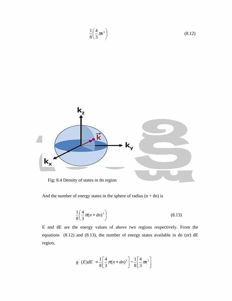
3

3

4

8

1nπ (8.12)

Fig: 8.4 Density of states in dn region

And the number of energy states in the sphere of radius (n + dn) is

+ 3)(3

4

8

1dnnπ (8.13)

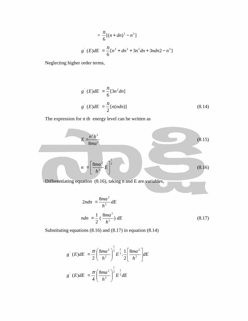
E and dE are the energy values of above two regions respectively. From the

equations (8.12) and (8.13), the number of energy states available in dn (or) dE

region,

−

+= 33'

3

4

8

1)(

3

4

8

1)( ndnndEEg ππ

= ])[(6

33 ndnn −+π

]233[6

)( 3233' nndndnndnndEEg −+++= π

Neglecting higher order terms,

]3[6

)( 2' dnndEEgπ=

)]([2

)(' ndnndEEgπ= (8.14)

The expression for n th energy level can be written as

2

22

8ma

hnE = (8.15)

2

1

2

28

= E

h

man (8.16)

Differentiating equation (8.16), taking n and E are variables,

dEh

mandn

2

282 =

dEh

mandn )

8(

2

12

2

= (8.17)

Substituting equations (8.16) and (8.17) in equation (8.14)

dEh

maE

h

madEEg

=

2

22

12

1

2

2' 8

2

1.

8

2)(

π

dEEh

madEEg 2

12

1

2

2' 8

4)(

= π

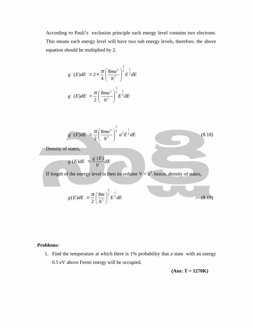
According ro Pauli’s exclusion principle each energy level contains two electrons.

This means each energy level will have two sub energy levels, therefore, the above

equation should be multiplied by 2.

dEEh

madEEg 2

12

3

2

2' 8

42)(

×= π

dEEh

madEEg 2

12

3

2

2' 8

2)(

= π

dEEah

madEEg 2

13

2

3

2

2' 8

2)(

= π

(8.18)

Density of states,

dEV

EgdEEg

)()(

'

=

If length of the energy level is then its volume V = a3. hence, density of states,

dEEh

mdEEg 2

12

3

2

8

2)(

= π (8.19)

Problems:

1. Find the temperature at which there is 1% probability that a state with an energy

0.5 eV above Fermi energy will be occupied.

(Ans: T = 1270K)

2. At what temperature we can except a 10% probability that electron in silver have

an energy which is 1% above the Fermi energy? The Fermi energy of silver is 5.5

eV. (Ans: T = 290.2K)

3. compute the average kinetic energy of a gas molecule at 300 C. Express the result

in election volts. If the gas is hydrogen. What is the order of magnitude of the

velocity of molecules at 300C?

(Ans: _

c = 6104.69 m/s)

4. calculate the velocity of an electron with kinetic energy of 10 electron volt; what

is the velocity of a proton with kinetic energy of 10 electron volt?

( Ans: −

−

−×=

××××= smc

kg

Jc pp /101616.19;

101.9

106.1102 1233

19

)

5. Find the drift velocity of free electron in a copper wire of cross sectional area 10

mm2 when the wire carries a current of 100A. assume that each copper atom

contributes one electron to the electron gas.

(Ans: ud =7.35294 x 104 m/s)

6. Calculate the energy of a of sodium light of wavelength 5893 x 10-10m in (a)

joules and (b) electron – volts (eV). Take h = 6.62 x 10-34 J-s and c = 3 x 108 m/s.

(Ans: 2.11eV)

7. A radio transmitter operates at a frequency of 880 kHz and a power of 10kW.

How many photons per seconds does it emit.

(Ans: 17.15 x 1030)

8. A mercury arc is rated at 200 W. How many light quanta are emitted per second

in radiation having wavelength of 6123A0 if the intensity of this line is 2% only.

Assume that 50% of power is spent for radiation.

(Ans: 6.16 x 1018)

9. A pulse of radiation consisting of 5 x 104 photons of 0

3000 A=λ falls on a

photosensitive surface whose sensitivity for this wavelength region is J = 5

mA/W. Find the number of photoelectrons liberated by the pulse.

(Ans: 1034)

10. a) How many photons of a radiation of wavelength =λ 5 x 10-7 m must fall per

second on a blackened metallic plate in order to produce a force of 10-5 newton?

b) At what rate will be the temperature of the plate rise if its mass is 1.5 gram and

specific heat 0.1? take h = 6062 x 10-34 J-s.?

(Ans: (a) 7.54 x 1021 b) 4.8 x 103 0C/s)

11. A blue lamp emits light of mean wavelength of 4500A0. The lamp is rated a

150W and 8% of the energy appears as emitted light. How many photons are

emitted by the lamp per second?

(Ans: 27.15x1018)

12. With what velocity mist an electron travel so that its momentum is equal to that of

a photon with a wavelength of 0

5200 A=λ ?

(Ans: p = 1400 m/s)