elements of high-performance reconfigurable · pdf fileelements of high-performance...
TRANSCRIPT

Elements of High-PerformanceReconfigurable Computing*
TOM VANCOURT†
Department of Electrical and Computer Engineering,
Boston University, Boston, Massachusetts 02215
MARTIN C. HERBORDT
Department of Electrical and Computer Engineering,
Boston University, Boston, Massachusetts 02215
Abstract
Numerous application areas, including bioinformatics and computational
biology (BCB), demand increasing amounts of processing capability. In many
cases, the computation cores and data types are suited to field-programmable
gate arrays (FPGAs). The challenge is identifying those design techniques that
can extract high performance from the FPGA fabric while allowing efficient
development of production-worthy program codes. After brief introductions to
high-performance reconfigurable computing (HPRC) systems and some appli-
cations for which they are well suited, we present a dozen such techniques
together with examples of their use in our own research in BCB. Each technique,
if ignored in a naive implementation, would have cost at least a factor 2 in
performance, with most saving a factor of 10 or more. We follow this by
comparing HPRC with an alternative accelerator technology, the use of graphics
processors for general-purpose computing (GPGPU). We conclude with a
discussion of some implications for future HPRC development tools.
* This chapter is based on two articles previously published by the IEEE: ‘‘Achieving High
Performance with FPGA-Based Computing’’ which appeared in IEEE Computer in March 2007, and
‘‘Computing Models for FPGA-Based Accelerators’’ which appeared in IEEE Computing in Science
and Engineering in November/December 2008.{ Currently with Altera, Inc.
ADVANCES IN COMPUTERS, VOL. 75 113 Copyright © 2009 Elsevier Inc.
ISSN: 0065-2458/DOI: 10.1016/S0065-2458(08)00802-4 All rights reserved.
Author's personalpersonal copycopy
1. Introduction . . . . . . . . . . . . . . . . . . . . . . . . . . . . . . . . . 115
2. FPGA Accelerator Architecture and Computing Models . . . . . . . . . . 117
2.1. Low-Level FPGA Models . . . . . . . . . . . . . . . . . . . . . . . . . . 117
2.2. FPGA Computation Basics . . . . . . . . . . . . . . . . . . . . . . . . . 119
3. Sample Applications . . . . . . . . . . . . . . . . . . . . . . . . . . . . . 120
3.1. Molecular Dynamics . . . . . . . . . . . . . . . . . . . . . . . . . . . . . 121
3.2. Multigrid for Electrostatic Computation . . . . . . . . . . . . . . . . . . . 121
3.3. Discrete Molecular Dynamics . . . . . . . . . . . . . . . . . . . . . . . . 123
3.4. Modeling Molecular Interactions (Docking) . . . . . . . . . . . . . . . . . 123
3.5. Sequence Alignment: Dynamic Programming-Based Methods . . . . . . . 124
3.6. Sequence Alignment: BLAST . . . . . . . . . . . . . . . . . . . . . . . . 124
3.7. Sequence Analysis Case Study: Finding Repetitive Structures . . . . . . . 125
3.8. Microarray Data Analysis Case Study: Finding Best Combinations . . . . . 125
3.9. Characteristics of Computations Amenable to FPGA Acceleration . . . . . 126
4. Methods for Avoiding
Implementational Heat . . . . . . . . . . . . . . . . . . . . . . . . . . . 127
4.1. Use an Appropriate FPGA Computing Model . . . . . . . . . . . . . . . . 128
4.2. Use an Appropriate FPGA Algorithm . . . . . . . . . . . . . . . . . . . . 132
4.3. Use Appropriate FPGA Structures . . . . . . . . . . . . . . . . . . . . . . 133
4.4. Mitigate Amdahl’s Law . . . . . . . . . . . . . . . . . . . . . . . . . . . 136
4.5. Hide Latency of Independent Functions . . . . . . . . . . . . . . . . . . . 136
4.6. Speed-Match Sequential Computations . . . . . . . . . . . . . . . . . . . 138
4.7. High Performance = High-Performance Data Access . . . . . . . . . . . . 139
4.8. Use Appropriate Arithmetic Precision . . . . . . . . . . . . . . . . . . . . 141
4.9. Use Appropriate Arithmetic Mode . . . . . . . . . . . . . . . . . . . . . . 142
4.10. Minimize Use of High-Cost Arithmetic . . . . . . . . . . . . . . . . . . . 143
4.11. Support Families of Applications Rather Than Point Solutions . . . . . . . 144
4.12. Scale Application for Maximal Use of Target Hardware . . . . . . . . . . 146
5. GPGPU An Alternative Approach to Acceleration . . . . . . . . . . . . . 148
5.1. Overview . . . . . . . . . . . . . . . . . . . . . . . . . . . . . . . . . . 148
5.2. Data Path Structure . . . . . . . . . . . . . . . . . . . . . . . . . . . . . 149
5.3. Memory Access . . . . . . . . . . . . . . . . . . . . . . . . . . . . . . . 150
5.4. Task Scheduling . . . . . . . . . . . . . . . . . . . . . . . . . . . . . . . 150
5.5. Comparison with HPRC . . . . . . . . . . . . . . . . . . . . . . . . . . . 151
6. Conclusion . . . . . . . . . . . . . . . . . . . . . . . . . . . . . . . . . . 152
114 T. VANCOURT AND M. C. HERBORDT
personal copy

1. Introduction
For many years computational scientists could depend on continual access to ever
faster computers. In the last few years, however, power concerns have caused
microprocessor operating frequencies to stagnate. Moreover, while advances in
process technology continue to provide ever more features per chip, these are no
longer used primarily to augment individual microprocessors; rather they are com-
monly used to replicate the CPUs. Production chips with hundreds of CPU cores are
projected to be delivered in the next several years. At the same time, however, it has
become clear that replicating cores is only one of several viable strategies for
developing next-generation high-performance computing (HPC) architectures.
Some promising alternatives are based on field-programmable gate arrays
(FPGAs) [25]. FPGAs are commodity integrated circuits (ICs) whose logic can be
determined, or programmed, in the field. This is in contrast to other classes of ICs
(e.g., application-specific integrated circuits—ASICs) whose logic is fixed at fabri-
cation time. The tradeoff is that FPGAs are less dense and fast than ASICs; often,
however, the flexibility more than makes up for these drawbacks. Applications
accelerated with FPGAs have often delivered 100-fold speedups per node
over microprocessor-based systems. This, combined with the current ferment in
computer architecture activity, has resulted in such systems moving toward the
mainstream, with integration support being provided by the largest vendors [6, 52].
The enormous potential performance derived from accelerating HPC applications
with FPGAs (high-performance reconfigurable computing—HPRC) comes from
two sources (1) parallelism—1000� is possible, especially for low-precision com-
putations and (2) payload per computation—since most control is configured into
the logic itself, overhead instructions (such as array indexing and loop computa-
tions) need not be emulated. On the other hand, there are significant, inherent,
challenges. One is the low operating frequency: an FPGA clocks at one tenth the
speed of a high-end microprocessor. Another is simply Amdahl’s law: to achieve the
speedup factors required for user acceptance of a new technology (preferably 50�[11]) close to 99% of the target application must lend itself to substantial accelera-
tion. As a result, performance of HPC applications accelerated with FPGA copro-
cessors is unusually sensitive to the quality of the implementation. Put another way,
the potential performance of HPRC is tremendous, but what users often find is that it
is much easier to get no speedup at all.
The problem described here is a classic one: how to achieve significant speedups
on a new architecture without expending exorbitant development effort, and while
retaining flexibility, portability, and maintainability. This problem is familiar
in porting uniprocessor applications to massively parallel processors (MPPs).
ELEMENTS OF HPRC 115
Author's personal copy
Two differences are as follows (1) FPGAs are far more different from uniprocessors
than MPPs are from uniprocessors and (2) the process of parallelizing code for
MPPs, while challenging, is still better understood and supported than porting codes
to FPGAs. The basic parameters for the ‘‘portability problem’’ (whether among
MPPs or other non-PC architectures) were stated by Snyder [64]. First, that a parallel
solution utilizing P processors can improve the best sequential solution by at most a
factor of P. Second, that HPC problems tend to have third- to fourth-order complex-
ity and so parallel computation, while essential, offers only modest benefit. And
finally, that therefore ‘‘the whole force of parallelism must be transferred to the
problem, not converted to ‘heat’ of implementational overhead.’’
The portability problem has been addressed variously over the last 40 years, with
well-known approaches involving language design, optimizing compilers, other
software engineering tools and methods, and function and application libraries
(see, e.g., last year’s Advances in Computers for some approaches used in DARPA’s
HPCS program [21, 24]). It is generally agreed that compromises are required: one
can restrict the variety of architectures, or the scope of application; or one can bound
expectations in performance, or in ease of implementation. The point in the spec-
trum we have chosen is as follows. For architecture, we assume a standard PC with
FPGA coprocessor on a high-speed bus. For performance, we aim to achieve at least
10� (with 50� the target) to motivate using a nonstandard architecture. For appli-
cations, we concentrate on those that are widely used, have high potential parallel-
ism, and, preferably, low precision. And finally, for effort, we consider from a few
programmer/designer months to 1 year or 2 (depending on application complexity
and potential impact) as being realistic. Our methods follow standard FPGA design
procedures, based primarily on the VHDL hardware description language (HDL)
augmented with our own LAMP tool suite [68, 69].
We continue this chapter with brief introductions to HPRC systems and some
applications for which they are well suited. The central part of this chapter
describes 12 methods we have used to avoid ‘‘generating implementational
heat’’ in our acceleration of several HPRC applications. Each, if ignored, would
have cost at least a factor of 2 in performance, with most saving a factor of 10 or
more. As many of these methods are well known to those experienced in the
HPRC, this survey is particularly targeted to the many newcomers to the field
who may wish to augment performance obtained through direct C-to-gates imple-
mentations. We follow this by comparing HPRC with an alternative accelerator
technology, the use of graphics processors (GPUs) for general-purpose computing
(GPGPU). We conclude with a discussion of the implications of these methods
to the design of the next generation of design tools. Integration into future HPRC
design processes appears to be readily achievable, and will not require HPRC
designers to become proficient in an HDL.
116 T. VANCOURT AND M. C. HERBORDT
Author's personal copy
2. FPGA Accelerator Architecture andComputing Models
FPGAs have been available since the 1980s, but have only recently started to
become popular as computation accelerators. To understand why, it is necessary to
understand something about their basic technology. That technology explains the
FPGAs’ strengths and limitations as application accelerators, shows why FPGA
programming is so different from traditional kinds of application programming, and
determines the applications likely to benefit from FPGA acceleration.
2.1 Low-Level FPGA Models
FPGAs are reprogrammable chips containing large numbers of configurable logic
gates, registers, and interconnections. FPGA programming means defining the bit-
level configuration of these resources to create a circuit that implements a desired
function. The FPGAs of interest store their configuration data in static RAM cells
distributed across the chip, so they can be reused indefinitely for different computa-
tions defined by different logic configurations.
While it is possible to program an FPGA by specifying settings of individual
components, this is rarely done for HPRC applications; if anything, HPRC devel-
opers are more willing to trade off performance for programmability by using the
highest possible level of abstraction. Still, the historic computing model is useful:
FPGAs are a ‘‘bag of gates’’ that can be configured into logic designs using HDLs
such as Verilog and VHDL.
In the last few years, high-end FPGAs have come to be dominated by embedded
components such as multipliers, independently addressable memories (block
RAMs—BRAMs), and high-speed I/O links. Aligned with these changes, a new
low-level computing model has emerged: FPGAs as a ‘‘bag of computer parts.’’
A designer using this model would likely consider the following FPGA features
when designing an application:
l Reconfigurable in milliseconds
l Hundreds of hardwired memories and arithmetic units
l Millions of gate-equivalents
l Millions of communication paths, both local and global
l Hundreds of gigabit I/O ports and tens of multigigabit I/O ports
l Libraries of existing designs analogous to the various system and application
libraries commonly used by programmers
ELEMENTS OF HPRC 117
Author's personal copy
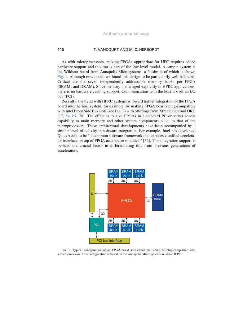
As with microprocessors, making FPGAs appropriate for HPC requires added
hardware support and this too is part of the low-level model. A sample system is
the Wildstar board from Annapolis Microsystems, a facsimile of which is shown
Fig. 1. Although now dated, we found this design to be particularly well balanced.
Critical are the seven independently addressable memory banks per FPGA
(SRAMs and DRAM). Since memory is managed explicitly in HPRC applications,
there is no hardware caching support. Communication with the host is over an I/O
bus (PCI).
Recently, the trend with HPRC systems is toward tighter integration of the FPGA
board into the host system, for example, by making FPGA boards plug-compatible
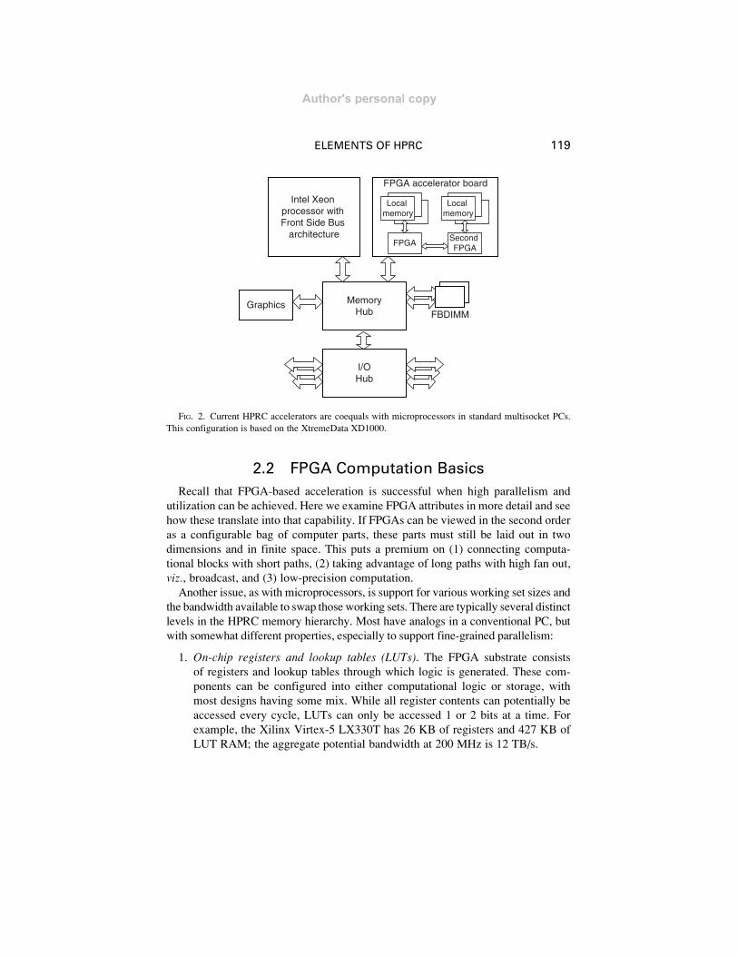
with Intel Front Side Bus slots (see Fig. 2) with offerings from XtremeData and DRC
[17, 54, 67, 78]. The effect is to give FPGAs in a standard PC or server access
capability to main memory and other system components equal to that of the
microprocessors. These architectural developments have been accompanied by a
similar level of activity in software integration. For example, Intel has developed
QuickAssist to be ‘‘a common software framework that exposes a unified accelera-
tor interface on top of FPGA accelerator modules’’ [52]. This integration support is
perhaps the crucial factor in differentiating this from previous generations of
accelerators.
32FPGA
SRAMbank
36 36 36
36 36 36
DRAMbank
PCI
32
PCI bus interface
I/O
SRAMbank
SRAMbank
SRAMbank
SRAMbank
SRAMbank
FIG. 1. Typical configuration of an FPGA-based accelerator that could be plug-compatible with
a microprocessor. This configuration is based on the Annapolis Microsystems Wildstar II Pro.
118 T. VANCOURT AND M. C. HERBORDT
Author's personal copy
2.2 FPGA Computation Basics
Recall that FPGA-based acceleration is successful when high parallelism and
utilization can be achieved. Here we examine FPGA attributes in more detail and see
how these translate into that capability. If FPGAs can be viewed in the second order
as a configurable bag of computer parts, these parts must still be laid out in two
dimensions and in finite space. This puts a premium on (1) connecting computa-
tional blocks with short paths, (2) taking advantage of long paths with high fan out,
viz., broadcast, and (3) low-precision computation.
Another issue, as with microprocessors, is support for various working set sizes and
the bandwidth available to swap those working sets. There are typically several distinct
levels in the HPRC memory hierarchy. Most have analogs in a conventional PC, but
with somewhat different properties, especially to support fine-grained parallelism:
1. On-chip registers and lookup tables (LUTs). The FPGA substrate consists
of registers and lookup tables through which logic is generated. These com-
ponents can be configured into either computational logic or storage, with
most designs having some mix. While all register contents can potentially be
accessed every cycle, LUTs can only be accessed 1 or 2 bits at a time. For
example, the Xilinx Virtex-5 LX330T has 26 KB of registers and 427 KB of
LUT RAM; the aggregate potential bandwidth at 200 MHz is 12 TB/s.
MemoryHub
FPGA accelerator board
FPGA
Local memory
Second FPGA
Local memory
Intel Xeon processor with Front Side Bus
architecture
FBDIMM
I/OHub
Graphics
FIG. 2. Current HPRC accelerators are coequals with microprocessors in standard multisocket PCs.
This configuration is based on the XtremeData XD1000.
ELEMENTS OF HPRC 119
Author's personal copy

2. On-chip BRAMs. High-end FPGAs have several hundred independently
addressable multiported BRAMs. For example, the Xilinx Virtex-5 LX330T
has 324 BRAMs with 1.5 MB total storage and each accessible with a word
size of up to 72 bits; the aggregate potential bandwidth at 200 MHz is 1.2 TB/s.
3. On-board SRAM. High-end FPGAs have hundreds of signal pins that can be
used for off-chip memory. Typical boards, however, have between two and six
32-bit independent SRAM banks, with recent boards, such as the SGI RASC
having close to 100 MB. As with the on-chip BRAMs, off-chip access is
completely random and per cycle. The maximum possible such bandwidth
for the Xilinx Virtex-5 LX330T is 49 GB/s, but a figure between 1.6 and 5 GB/s
is more common.
4. On-board DRAM. Many boards either also have DRAM or replace SRAM
completely with DRAM. Recent boards support multiple GB of DRAM. The
bandwidth numbers are similar to those with SRAM, but with higher access
latency.
5. Host memory. Several recent boards support high-speed access to host memory
through, for example, SGI’s NumaLink, Intel’s Front Side Bus, and Hypertran-
sport used by AMD systems. Bandwidth of these links ranges from 5 to 20 GB/s
or more.
6. High-speed I/O links. FPGA applications commonly involve high-speed
communication. High-end Xilinx FPGAs have up to 24 3 GB/s ports.
The actual performance naturally depends on the existence of configurations that
can use this bandwidth. In our own work, we frequently use the entire available
BRAM bandwidth, and almost as often use most of the available off-chip bandwidth
as well. In fact, we interpret this achievement for any particular application as an
indication that we are on target with our mapping of application to hardware.
3. Sample Applications
Any computing platform works better for some applications than for others, partly
because of the physical structure of the computing hardware and partly due to the
computational characteristics of the application. This section serves two purposes.
The first is to put in a single place outlines of the applications used as case studies
in our description of implementation methods. The second is to show the character-
istics of applications that are good candidates for FPGA acceleration. We first
describe a number of applications we have accelerated, and then summarize their
applicable characteristics.
120 T. VANCOURT AND M. C. HERBORDT
Author's personal copy

3.1 Molecular Dynamics
Molecular dynamics (MD) is an iterative application of Newtonian mechanics to
ensembles of atoms and molecules (for more detail, see, e.g., Rapaport [58] or Haile
[31]). Time steps alternate between force computation and motion integration.
The short- and long-range components of the nonbonded force computation domi-
nate execution. As they have very different character, especially when mapped to
FPGAs, we consider them separately. The short-range force part, especially, has
been well studied for FPGA-based systems (see, e.g., [1, 3, 28, 41, 61, 76]).
MD forces may include van der Waals attraction and Pauli repulsion (approxi-
mated together as the Lennard–Jones, or LJ, force), Coulomb, hydrogen bond, and
various covalent bond terms:
Ftotal ¼ Fbond þ Fangle þ Ftorsion þ FH�bond þ Fnonbonded: ð1ÞBecause the hydrogen bond and covalent terms (bond, angle, and torsion) affect
only neighboring atoms, computing their effect is O(N) in the number of particles
N being simulated. The motion integration computation is alsoO(N). Although some
of these O(N) terms are easily computed on an FPGA, their low complexity makes
them likely candidates for host processing, which is what we assume here. The LJ
force for particle i can be expressed as:
FLJi ¼
Xj 6¼i
eabs2ab
12sabjrjij� �14
� 6sabjrjij� �8( )
rji; ð2Þ
where eab and sab are parameters related to the types of particles, that is, particle i istype a and particle j is type b. The Coulombic force can be expressed as:
FCi ¼ qi
Xj6¼i
qj
jrjij3 !
rji: ð3Þ
In general, the forces between all particle pairs must be computed leading to an
undesirable O(N2) complexity. The common solution is to split the nonbonded forces
into two parts: a fast converging short-range part, which consists of the LJ force and the
nearby component of the Coulombic, and the remaining long-range part of the
Coulombic (which is described in Section 3.2). The complexity of the short-range force
computation is then reduced toO(N) by only processing forces among nearby particles.
3.2 Multigrid for Electrostatic Computation
Numerous methods reduce the complexity of the long-range force computation
from O(N2) to O(N log N), often by using the fast Fourier transform (FFT). As these
have so far proven difficult to map efficiently to FPGAs, however, the multigrid
ELEMENTS OF HPRC 121
Author's personal copy
method may be preferable [26] (see, e.g., [9, 37, 60, 62] for its application to
electrostatics).
The difficulty with the Coulombic force is that it converges too slowly to restrict
computation solely to proximate particle pairs. The solution begins by splitting the
force into two components, a fast converging part that can be solved locally without
loss of accuracy, and the remainder. This splitting appears to create an even more
difficult problem: the remainder converges more slowly than the original. The key
idea is to continue this process of splitting, each time passing the remainder on to the
next coarser level, where it is again split. This continues until a level is reached
where the problem size (i.e., N) is small enough for the direct all-to-all solution to
be efficient.
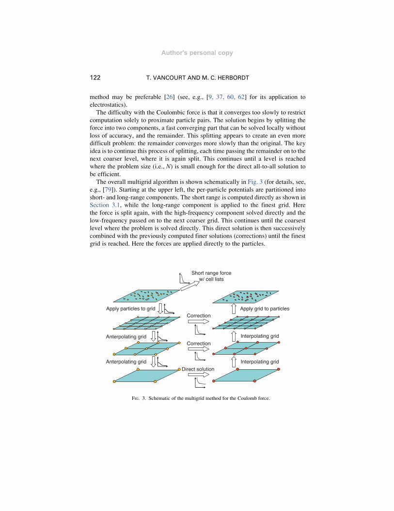
The overall multigrid algorithm is shown schematically in Fig. 3 (for details, see,
e.g., [79]). Starting at the upper left, the per-particle potentials are partitioned into
short- and long-range components. The short range is computed directly as shown in
Section 3.1, while the long-range component is applied to the finest grid. Here
the force is split again, with the high-frequency component solved directly and the
low-frequency passed on to the next coarser grid. This continues until the coarsest
level where the problem is solved directly. This direct solution is then successively
combined with the previously computed finer solutions (corrections) until the finest
grid is reached. Here the forces are applied directly to the particles.
Apply particles to grid
Anterpolating grid
Anterpolating grid
Direct solution
Correction
Correction
Interpolating grid
Interpolating grid
Apply grid to particles
Short range forcew/ cell lists
FIG. 3. Schematic of the multigrid method for the Coulomb force.
122 T. VANCOURT AND M. C. HERBORDT
Author's personal copy

3.3 Discrete Molecular Dynamics
Increasingly popular is MD with simplified models, such as the approximation of
forces with stepwise potentials (see, e.g., [58]). This approximation results in
simulations that advance by discrete event rather than time step. The foundation
of discrete molecular dynamics (DMD) is intuitive, hypothesis-driven, modeling
based on tailoring simplified models to the physical systems of interest [19]. Using
intuitive models, simulation length and time scales can exceed those of time step-
driven MD by eight or more orders of magnitude [20]. Even so, not only is DMD still
compute bound, causality concerns make it difficult to scale to a significant number
of processors. An efficient mapping to FPGAs is described in [34, 53].
Discrete event simulation (DES) is sketched in Fig. 4: the primary components are
the event queue, event processor, event predictor (which can also cancel previously
predicted events), and system state. Parallelization of DES has generally taken one
of two approaches (1) conservative, which guarantees causal order, or (2) optimistic,
which allows some speculative violation of causality and corrects violations with
rollback. Neither approach has worked well for DMD. The conservative approach,
which relies on there being a ‘‘safe’’ window, falters because in DMD there is none.
Processed events invalidate predicted events anywhere in the event queue with equal
probability, and potentially anywhere in the simulated space. For similar reasons,
the optimistic approach has frequent rollbacks, resulting in poor scaling.
3.4 Modeling Molecular Interactions (Docking)
Noncovalent bonding between molecules, or molecular docking, is basic to the
processes of life and to the effectiveness of pharmaceuticals (see, e.g., [42] for a
survey and [65, 71, 74] for FPGA implementations). While detailed chemical
Time-orderedevent queue
arbitrary insertionsand deletions
Eventprocessor
Eventpredictor
(and remover)
Systemstate
Events
New stateinfo
Stateinfo Events and
invalidations
FIG. 4. Block diagram of a typical discrete event simulation.
ELEMENTS OF HPRC 123
Author's personal copy
models are sometimes used, such techniques are computationally exorbitant and
infeasible for answering the fundamental question: at what approximate offsets and
orientations could the molecules possibly interact at all? Less costly techniques are
used for initial estimates of the docked pose, the relative offset and rotation that give
the strongest interaction. Many applications assume rigid structure as a simplifying
approximation: 3D voxel grids represent the interacting molecules and 3D correla-
tion is used for determining the best fit [39]. This is the specific application we
address here.
3.5 Sequence Alignment: Dynamic
Programming-Based Methods
A fundamental abstraction in bioinformatics represents macromolecules such as
proteins and DNA with sequences of characters. Bioinformatics applications use
sequence alignment (approximate string matching) to find similarities among mole-
cules that have diverged through mutation and evolution (for more detail, see, e.g.,
Durbin et al. [22] or Gusfield [30]). For two sequences of length m and n, dynamic
programming (DP)-based methods (such as Needleman–Wunsch and Smith–Water-
man) build an m � n-table of character–character match scores. The table is then
traversed using a recurrence relation where the score of each cell Si, j depends onlyon the scores of cells Si; j�1, Si�1; j, and Si�1; j�1. The serial complexity is O(mn).
DP-based can be implemented in hardware with a one-dimensional systolic array
of processing elements (PEs). In a simple case, the length m-sequence is held in
the array, one character per PE, while the length n-sequence streams through.
The hardware complexity is O(n); there have been many such implementations
[7, 8, 14, 23, 29, 35, 49, 50, 59, 73, 80].
3.6 Sequence Alignment: BLAST
Although O(mn) for sequence alignment is a remarkable improvement over the
naive algorithms, which have unbounded complexity, it is still far too great for large
databases. A heuristic algorithm, BLAST, generally runs in O(n) time, and is often
sufficiently sensitive (see, e.g., [2, 44] for details). BLAST is based on an observa-
tion about the typical distribution of high-scoring character matches in the DP
alignment table: There are relatively few overall, and only a small fraction are
promising. This promising fraction is often recognizable as proximate line segments
parallel to the main diagonal.
We now sketch the classic BLAST algorithm [2]. There are three phases: identi-
fying contiguous high scores (parallel to the main diagonal), extending them along
124 T. VANCOURT AND M. C. HERBORDT
Author's personal copy
the diagonal, and attempting to merge nearby extensions, which may or may not be
on the same diagonal. The third phase, which accounts for gaps, is nowadays often
replaced by a pass of Smith–Waterman on the regions of the database identified as of
possible interest. The O(mn) complexity of Smith–Waterman is not as significant
when only run on small parts of the database; for example, Krishnamurthy et al. [45]find that, for a set of BLASTn experiments, the final pass accounts for well under 1%
of the run time. This (effectively) makes the final pass O(m2), where m� n. Therehave been several FPGA implementations of BLAST (see, e.g., [13, 32, 38, 55]).
3.7 Sequence Analysis Case Study: Finding
Repetitive Structures
Another important bioinformatics task is analyzing DNA or protein sequences for
patterns that might be indicative of disease or be otherwise fundamental to cell
processes. These patterns are typically repetitive structures, such as tandem arrays
and palindromes, under various mismatch models [5, 30, 46]. The asymptotically
optimal algorithms are often based on suffix trees; practical algorithms often include
heuristics. Some of the hardware structures useful for HPRC in finding repetitive
structures are either obvious or go back decades; Conti et al. [15] describe some of
these and several extensions.
3.8 Microarray Data Analysis Case Study:
Finding Best Combinations
Microarrays, sometimes called ‘‘gene chips,’’ measure the expression products of
thousands of genes in a tissue sample and so are being used to investigate a number of
critical biological questions (see, e.g., [4, 43, 77]). Typical questions microarrays are
used to answer involve finding relationships among gene expressions, therapeutic
agents, and patient outcomes. Although a remarkably powerful tool, the analysis of the
resulting data is extremely challenging. Data are low precision ( just a few bits), noisy,
and sometimes missing altogether. The number of microarrays is invariably much
smaller than the data per microarray leading to underconstrained systems not amena-
ble to traditional statistical analysis such as finding correlations. More common are
various forms of clustering, inference nets, and decision trees.
In one study, Kim et al. [40] would like to find a set of genes whose expression
could be used to determine whether liver samples are metastatic on not. For
biological reasons, it is likely that three genes is an appropriate number to make
this determination. Kim et al. further propose that use of linear regression would
be appropriate to evaluate the gene subsets over the available samples. Since there
ELEMENTS OF HPRC 125
Author's personal copy

are tens of thousands of potential genes, 1011–1012 data subsets need to be pro-
cessed. Although simple to implement, he reported that this computation was
intractable even on his small cluster of PCs. We found that this algorithm could
be implemented extremely efficiently on an FPGA [75] (see also [57] for the
application of FPGAs in using microarray data for learning gene regulatory net-
works). While this combinatoric algorithm has not found widespread use, the FPGA
case study illustrates the methods central to microarray computation, including
handling noisy low-precision data, reducing large vector spaces, and applying
basic operators in linear algebra.
3.9 Characteristics of Computations Amenable
to FPGA Acceleration
We now summarize the characteristics of computations amenable to FPGA
acceleration:
l Massive, open-ended parallelism. HPRC applications are highly parallel, with
the possibility of thousands of operations being executed concurrently. Many
HPRC applications also feature open-ended parallelism, in the sense that there
is effectively no upper bound on the number of PEs that can be applied to the
calculation. These applications map well onto devices with thousands of con-
current PEs. For example, processing of long strings parallelizes at the charac-
ter level, and grid-based molecule interactions parallelize at the level of grid
cells. Many HPRC applications share this level of parallelism, despite their
different basic units of computation.
l Dense, regular communication patterns. Communication is generally regular
and local: on any iteration, data only need to be passed to adjacent PEs.
The FPGA’s large number of communication paths ensures that all PEs can
send and receive data every cycle, while the local communication ensures low
latency. For example, string processing, alignment by dynamic programming,
3D correlation, and other applications all meet this description. This allows
well-understood hardware techniques to be employed, including systolic arrays
and pipelines with hundreds or thousands of steps.
l Modest working sets and deterministic data access. Although HPRC data sets
can be large, they are often amenable to partitioning and to heavy reuse of data
within partitions. When the working sets are too large to fit on-chip, they
usually have predictable reference patterns. This allows the relatively high
latency of off-chip transfers to be hidden by the high off-chip bandwidth
(500 signal pins). In extreme cases, such as when processing large databases,
126 T. VANCOURT AND M. C. HERBORDT
Author's personal copy
data can be streamed through the FPGA at multi-Gb rates by using the dedi-
cated I/O transceivers.
l Data elements with small numbers of bits. Reducing the precision of the
function units to that required by the computation allows the FPGA to be
configured into a larger number of function units. Many HPRC applications
naturally use small data values, such as characters in the four-letter nucleotide
alphabet, or bits and fixed-point values for grid models of molecules. Although
standard implementations generally use floating point, analysis often shows
that simpler values work equally well.
l Simple processing kernels. Many HPRC computations are repetitive with
relatively simple processing kernels being repeated large numbers of times.
The fine-grained resource allocation within an FPGA allocates only as many
logic resources as needed to each PE. Simpler kernels, requiring less logic each,
allow more PEs to be built in a given FPGA. This tradeoff of computation
complexity versus processor parallelism is not available on fixed processors.
As already stated, HPRC calculations often benefit from large computing
arrays, and PEs within the arrays are typically simple.
l Associative computation. FPGA hardware works well with common associative
operators: broadcast, match, reduction, and leader election. In all of these cases,
FPGAs can be configured to execute the associative operator using the long
communication pathways on the chip. The result is that, rather than being a
bottleneck, these associative operators afford perhaps the greatest speedup of
all: processing at the speed of electrical transmissions.
Not all problems work well in FPGAs. Those requiring high-precision floating-
point calculations often consume so many logic resources that there is little oppor-
tunity for on-chip parallelism. In many cases, however, applications implemented in
double-precision floating point on standard processor can be reimplemented in
reduced precision, fixed point, or other arithmetic, with little or no cost in accuracy.
4. Methods for AvoidingImplementational Heat
These 12 methods were selected for easy visualization; they are neither exhaus-
tive nor disjoint. Also, we have avoided low-level issues related to logic design and
synthesis that are well known in electronic design automation, and high-level issues
such as partitioning that are well known in parallel processing. The focus is on our
ELEMENTS OF HPRC 127
Author's personal copy

own work in bioinformatics and computational biology (BCB), but applies also
to other standard FPGA domains such as signal and image processing.
4.1 Use an Appropriate FPGA Computing Model
4.1.1 Overview
In recent work [33], we have addressed the fact that while HPRC has tremendous
potential performance, few developers of HPC applications have thus far developed
FPGA-based systems. One reason, besides the newness of their viability, is that
FPGAs are commonly viewed as hardware devices and thus require use of alien
development tools. Another is that new users may disregard the hardware altogether
by translating serial codes directly into FPGA configurations (using one of many
available tools; see, e.g., [36] for a survey). While this results in rapid development,
it may also result in unacceptable loss of performance when key features are not
used to their capability.
We have found that successful development of HPRC applications requires a
middle path: that the developer must avoid getting caught up in logic details, but at
the same time should keep in mind an appropriate FPGA-oriented computing model.
There are several such models for HPRC; moreover, they differ significantly from
models generally used in HPC programming (see, e.g., [16, 64]). For example,
whereas parallel computing models are often based on thread execution and inter-
action, FPGA computing can take advantage of additional degrees of freedom than
available in software. This enables models based on the fundamental characteristics
from which FPGAs get their capability, including highly flexible fine-grained
parallelism and associative operations such as broadcast and collective response
(see DeHon et al. [18] for a perspective of these issues from the point of view of
design patterns).
Putting this idea together with FPGA characteristics described earlier: A good
FPGA computing model is one that lets us create mappings that make maximal use
of available hardware. This often includes one or more levels of the FPGA memory
hierarchy. These mappings commonly contain large amounts of fine-grained paral-
lelism. PEs are often connected as either a few long pipelines (sometimes with 50
stages or more), or broadside with up to a few hundred very short pipelines.
Another critical factor in finding a good FPGA model is that code size translates
into FPGA area. The best performance is, of course, achieved if the entire FPGA
is used continuously, usually through fine-grained parallelism as just described.
Conversely, if a single pipeline does not fit on the chip, performance may be poor.
Poor performance can also occur with applications that have many conditional
computations. For example, consider a molecular simulation where determining
128 T. VANCOURT AND M. C. HERBORDT
Author's personal copy

the potential between pairs of particles is the main computation. Moreover, let the
choice of function to compute the potential depend on the particles’ separation. For a
microprocessor, invoking each different function probably involves little overhead.
For an FPGA, however, this can be problematic: each function takes up part of the
chip, whether it is being used or not. In the worst case, only a fraction of the FPGA is
ever in use. Note that all may not be lost: it may still be possible to maintain high
utilization by scheduling tasks among the functions and reconfiguring the FPGA
as needed.
Finally, while FPGA configurations resemble high-level language programs, they
specify hardware, not software. Since good computing models for software are not
necessarily good computing models for hardware, it follows that restructuring an
application can often substantially improve its performance. For example, while
random access and pointer-based data structures are staples of serial computing,
they may yield poor performance on FPGAs. Much preferred are streaming, systolic
and associative computing, and arrays of fine-grained automata.
4.1.2 Examples
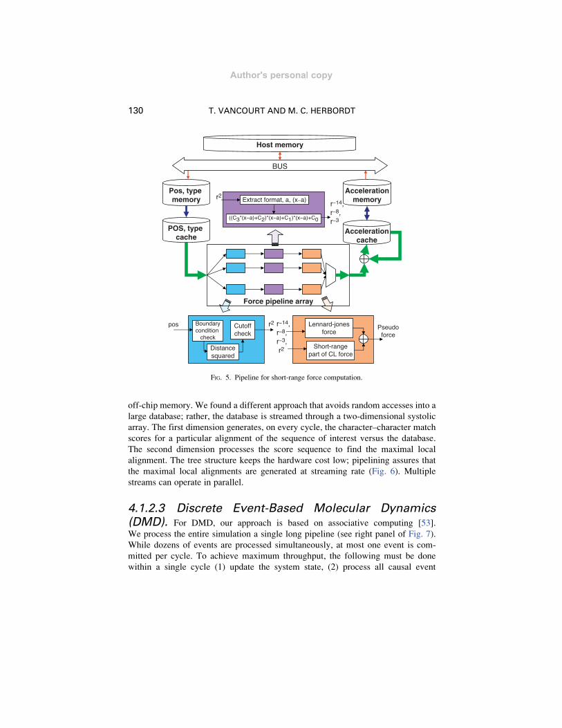
4.1.2.1 Molecular Dynamics: Short-Range Forces. The
short-range force kernel can be mapped into a streaming model [28]; this is illu-
strated in Fig. 5. Particle positions and types are the input, the accelerations the
output. Streams source and sink in the BRAMs. The number of streams is a function
of FPGA hardware resources and the computation parameters, with the usual range
being from 2 to 8.
The wrapper around this kernel is also implemented in the FPGA: it ensures that
particles in neighborhoods are available together in the BRAMs; these are swapped
in the background as the computation progresses. The force computation has three
parts, as shown in blue, purple, and orange, respectively. The first part checks for
validity, adjusts for boundary conditions, and computes r2. The second part com-
putes the exponentials in r. As is often done even in serial MD codes, these terms are
not computed directly, but rather with table lookup followed by interpolation. Third
order is shown in Fig. 5. The final part combines the r�n terms with the particle type
coefficients to generate the force.
4.1.2.2 Sequence Alignment Using BLAST. Recall that theBLAST algorithm, which operates in multiple phases. First seeds, or good matches
of short subsequences, are determined. Second, these seeds are extended to find
promising candidates. The direct mapping of this algorithm onto the FPGA
is dominated by the extension phase, which requires many random accesses into
ELEMENTS OF HPRC 129
personal copy
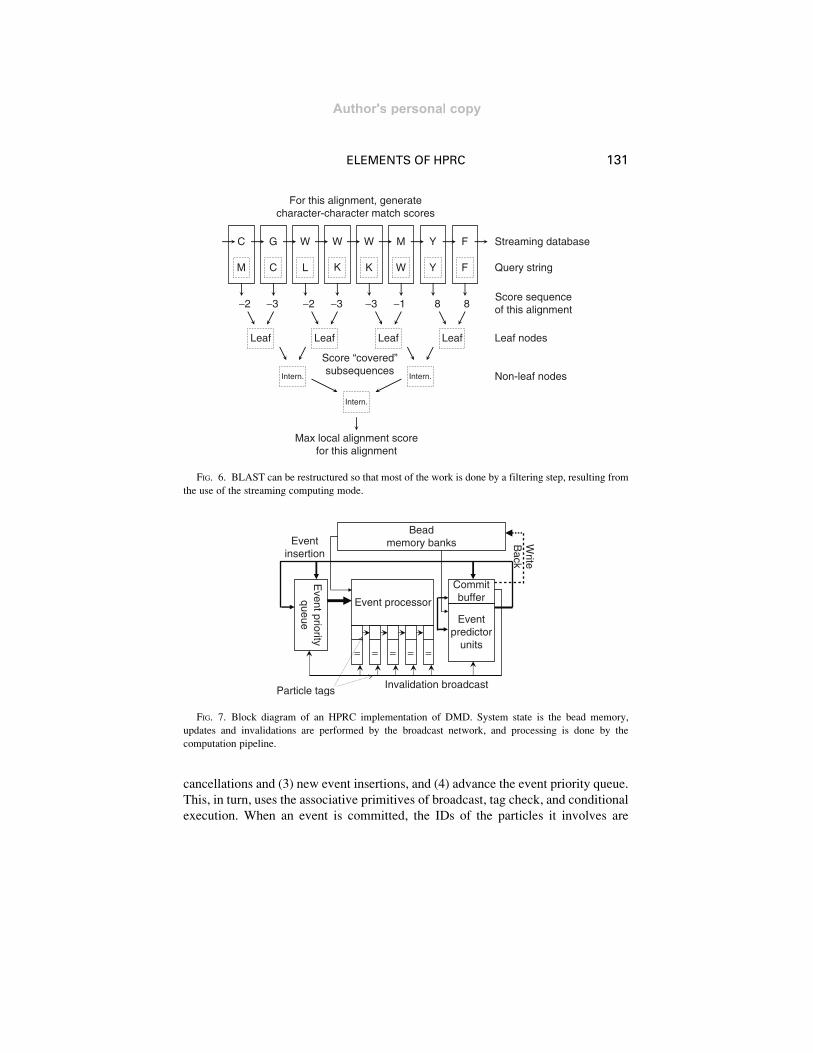
off-chip memory. We found a different approach that avoids random accesses into a
large database; rather, the database is streamed through a two-dimensional systolic
array. The first dimension generates, on every cycle, the character–character match
scores for a particular alignment of the sequence of interest versus the database.
The second dimension processes the score sequence to find the maximal local
alignment. The tree structure keeps the hardware cost low; pipelining assures that
the maximal local alignments are generated at streaming rate (Fig. 6). Multiple
streams can operate in parallel.
4.1.2.3 Discrete Event-Based Molecular Dynamics
(DMD). For DMD, our approach is based on associative computing [53].
We process the entire simulation a single long pipeline (see right panel of Fig. 7).
While dozens of events are processed simultaneously, at most one event is com-
mitted per cycle. To achieve maximum throughput, the following must be done
within a single cycle (1) update the system state, (2) process all causal event
pos
r2
r2 r−14,r−8,r−3, r2
r−14,r−8,r−3
Force pipeline array
Pos, type memory
Accelerationmemory
POS, type cache
Accelerationcache
BUS
Host memory
Boundarycondition
check
Cutoffcheck
Distancesquared
Extract format, a, (x−a)
((C3*(x−a)+C2)*(x−a)+C1)*(x−a)+C0
Lennard-jonesforce
Short-rangepart of CL force
Pseudoforce
FIG. 5. Pipeline for short-range force computation.
130 T. VANCOURT AND M. C. HERBORDT
Author's personal copy
cancellations and (3) new event insertions, and (4) advance the event priority queue.
This, in turn, uses the associative primitives of broadcast, tag check, and conditional
execution. When an event is committed, the IDs of the particles it involves are
M C
G
L
W
K
W
K
W
W
M
Y
Y
F
FC
Leaf Leaf Leaf Leaf
Intern. Intern.
Intern.
Max local alignment scorefor this alignment
Streaming database
Query string
Score sequenceof this alignment
Leaf nodes
Non-leaf nodes
Score “covered”subsequences
For this alignment, generatecharacter-character match scores
−2 −3 −2 −3 −3 −1 8 8
FIG. 6. BLAST can be restructured so that most of the work is done by a filtering step, resulting from
the use of the streaming computing mode.
CommitbufferEvent processor
Eventpredictor
units
Particle tags
= = = =
Invalidation broadcast
Beadmemory banks
Event priority
queue
Write
Back
Eventinsertion
=
FIG. 7. Block diagram of an HPRC implementation of DMD. System state is the bead memory,
updates and invalidations are performed by the broadcast network, and processing is done by the
computation pipeline.
ELEMENTS OF HPRC 131
Author's personal copy
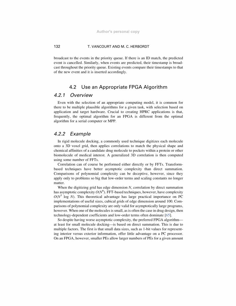
broadcast to the events in the priority queue. If there is an ID match, the predicted
event is cancelled. Similarly, when events are predicted, their timestamp is broad-
cast throughout the priority queue. Existing events compare their timestamps to that
of the new event and it is inserted accordingly.
4.2 Use an Appropriate FPGA Algorithm
4.2.1 Overview
Even with the selection of an appropriate computing model, it is common for
there to be multiple plausible algorithms for a given task, with selection based on
application and target hardware. Crucial to creating HPRC applications is that,
frequently, the optimal algorithm for an FPGA is different from the optimal
algorithm for a serial computer or MPP.
4.2.2 Example
In rigid molecule docking, a commonly used technique digitizes each molecule
onto a 3D voxel grid, then applies correlations to match the physical shape and
chemical affinities of a candidate drug molecule to pockets within a protein or other
biomolecule of medical interest. A generalized 3D correlation is then computed
using some number of FFTs.
Correlation can of course be performed either directly or by FFTs. Transform-
based techniques have better asymptotic complexity than direct summation.
Comparisons of polynomial complexity can be deceptive, however, since they
apply only to problems so big that low-order terms and scaling constants no longer
matter.
When the digitizing grid has edge dimension N, correlation by direct summation
has asymptotic complexityO(N6). FFT-based techniques, however, have complexity
O(N3 log N). This theoretical advantage has large practical importance on PC
implementations of useful sizes, cubical grids of edge dimension around 100. Com-
parisons of polynomial complexity are only valid for asymptotically large programs,
however. When one of the molecules is small, as is often the case in drug design, then
technology-dependent coefficients and low-order terms often dominate [65].
So despite having worse asymptotic complexity, the preferred FPGA algorithm—
at least for small molecule docking—is based on direct summation. This is due to
multiple factors. The first is that small data sizes, such as 1-bit values for represent-
ing interior versus exterior information, offer little advantage on a PC processor.
On an FPGA, however, smaller PEs allow larger numbers of PEs for a given amount
132 T. VANCOURT AND M. C. HERBORDT
Author's personal copy
of computing fabric, and products of 1-bit values are trivial to implement. Second,
efficient systolic arrays for correlation are well known. The form we chose requires
one input value and generates one output value per cycle, while holding partial sums
in on-chip registers and RAM-based FIFOs. Hundreds of dual-ported, on-chip
RAMs hold intermediate results, eliminating that as a potential bottleneck. Third,
our implementation (after a brief setup phase) delivers one multiply-accumulate
(MAC) operation per clock cycle per PE, with hundreds to thousands of PEs in the
computing array. No additional cycles are required for indexing, loop control, load/
store operations, or memory stalls. Despite clock rates at least 10� lower than a
PC’s, the FPGA executes thousands of times more payload computations per cycle.
As an aside, we observe that direct summation creates research opportunities that
were considered infeasible using transform-based techniques. FFTs handle only stan-
dard correlation, involving sums of products. Although complex chemical effects are
modeled by summing multiple correlations of different molecular features, FFTs
require every model to be phrased somehow as sums of a � b. Direct summation
makes it easy to perform a generalized sum-of-F(a, b) operation, where F computes an
arbitrary and possibly nonlinear score for the interaction of the two voxels from the two
molecules. It also allows arbitrary (and possibly different) data types for representing
voxels from the twomolecules.We commonly represent voxels as tupleswith fields for
steric effects, short-range forces, Coulombic interaction, or other phenomena.
4.3 Use Appropriate FPGA Structures
4.3.1 Overview
Certain data structures such as stacks, trees, and priority queues are ubiquitous in
application programs, as are basic operations such as search, reduction, parallel
prefix, and suffix trees. Digital logic often has analogs to these structures and
operations that are equally well known to logic designers. They are also completely
different from what is obtained by translating the software structures to hardware
using an HDL. The power of this method is twofold: to use such structures when
called for, and to steer the mapping toward those structures with the highest relative
efficiency. One particular hardware structure is perhaps the most commonly used in
all HPRC: the systolic array used for convolutions and correlations (see, e.g., [66]).
4.3.2 Examples
4.3.2.1 Multigrid for Electrostatic Computation. When
mapping multigrid to an FPGA, we partition the computation into three functions
(1) applying the charges to a 3D grid, (2) performing multigrid to convert the 3D
ELEMENTS OF HPRC 133
Author's personal copy

charge density grid to a 3D potential energy grid, and (3) applying the 3D potential to
the particles to compute the forces. The two particle–grid functions are similar enough
to be considered together, as are the various phases of the grid–grid computations. For
the 3D grid–grid convolutions we use the well-known systolic array. Its iterative
application to build up two- and three-dimensional convolvers is shown in Fig. 8.
In the basic 1D systolic array, shown in Fig. 8A, the kernel A[0. . .L] is held in thePEs and the new elements of the ‘‘signal’’ B[i] are broadcast to the array, one per
iteration. At each PE, the B[i] are combined with the A[k]; the result is added to the
running sum. The running sums are then shifted, completing the iteration. One result
is generated per iteration. The same basic procedure is used for the 2D and 3D cases
(shown in Fig. 8B and C), but with delay FIFOs added to account for difference in
sizes of A and B.
S
FIFO
FIFO
FIFO
bij
bijkaij3
aij2
aij1
aij0
FIFO
FIFO
FIFO
S
a32a33
... …
... … C[k]
A[L]
B[i]
0
A[L-1] A[0]A[L-2]
PE
A[k]
Init_A
a31 a30
a22a23 a21 a20
a12a13 a11 a10
a02a03 a01 a00
B
A
C
FIG. 8. Shown are (A) a one-dimensional systolic convolver array, and its extension to (B) two, and to
(C) three dimensions.
134 T. VANCOURT AND M. C. HERBORDT
Author's personal copy
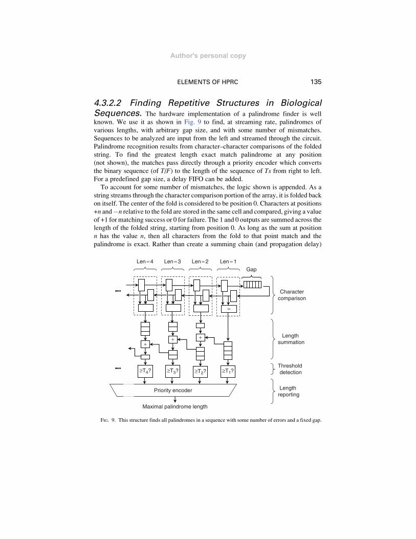
4.3.2.2 Finding Repetitive Structures in Biological
Sequences. The hardware implementation of a palindrome finder is well
known. We use it as shown in Fig. 9 to find, at streaming rate, palindromes of
various lengths, with arbitrary gap size, and with some number of mismatches.
Sequences to be analyzed are input from the left and streamed through the circuit.
Palindrome recognition results from character–character comparisons of the folded
string. To find the greatest length exact match palindrome at any position
(not shown), the matches pass directly through a priority encoder which converts
the binary sequence (of T/F) to the length of the sequence of Ts from right to left.
For a predefined gap size, a delay FIFO can be added.
To account for some number of mismatches, the logic shown is appended. As a
string streams through the character comparison portion of the array, it is folded back
on itself. The center of the fold is considered to be position 0. Characters at positions
+n and�n relative to the fold are stored in the same cell and compared, giving a value
of +1 for matching success or 0 for failure. The 1 and 0 outputs are summed across the
length of the folded string, starting from position 0. As long as the sum at position
n has the value n, then all characters from the fold to that point match and the
palindrome is exact. Rather than create a summing chain (and propagation delay)
Gap
+++
≥T4? ≥T3?
Priority encoder
Maximal palindrome length
= = ==
Len=1Len=2Len=3Len=4
Charactercomparison
Length summation
Threshold detection
Length reporting
≥T2? ≥T1?
FIG. 9. This structure finds all palindromes in a sequence with some number of errors and a fixed gap.
ELEMENTS OF HPRC 135
Author's personal copy
the full length of the character comparison array, this implementation pipelines
summation so that only one addition is performed per clock cycle. Summation results
are lagged so that all of the length totals for a single time step exit the length
summation section together.
4.4 Mitigate Amdahl’s Law
4.4.1 Overview
Amdahl’s law states that speeding up an application significantly through an
enhancement requires most of the application to be enhanced. This is sometimes
difficult to achieve with existing HPC code; for example, profiling has pointed to
kernels comprises just 60–80% of execution time when much more could have been
expected (as was found, e.g., by Alam et al. [1] in their MD application). The
problem is especially severe with legacy codes and may require a substantial rewrite.
Not all is lost, however. The nonkernel code may lend itself to substantial improve-
ment; as its relative execution time decreases, expending effort on its optimization
may become worthwhile. Also, combining computations not equally amenable to
FPGA acceleration may have optimized the original code; separating them can
increase the acceleratable kernel.
4.4.2 Example
Molecular dynamics codes are often highly complex and often have legacies
extending over decades (see, e.g., [10, 12]). While these codes sometimes extend to
millions of lines, the acceleratable kernels are much smaller. Various approaches have
been used. These include writing the MD code from scratch [61]; using a simplified
version of an existing standard, in this case NAMD [41]; accelerating what is possible
in an existing standard, in this case AMBER [63]; and using a code already designed
for acceleration, for example, ProtoMol [28]. In the last case the ProtoMol framework
was designed especially for computational experimentation and so has well-defined
partitions among computations [51]. We have found that the acceleratable kernel not
only comprises more than 90% of execution time with ProtoMol, but the modularity
enables straightforward integration of an FPGA accelerator [28].
4.5 Hide Latency of Independent Functions
4.5.1 Overview
Latency hiding is a basic technique for obtaining high performance in parallel
applications. Overlap between computation and communication is especially desir-
able. In FPGA implementations, further opportunities arise: rather than allocating
136 T. VANCOURT AND M. C. HERBORDT
Author's personal copy
tasks to processors among which communication is then necessary, functions are
simply laid out on the same chip and operate in parallel.
Looking at this in a little more detail, while having function units lying idle is
the bane of HPRC, functional parallelism can also be one its strengths. Again, the
opportunity has to do with FPGA chip area versus compute time: functions that take
a long time in software, but relatively little space in hardware are the best.
For example, a simulator may require frequent generation of high-quality random
numbers. Such a function takes relatively little space on an FPGA, can be fully
pipelined, and can thus provide random numbers with latency completely hidden.
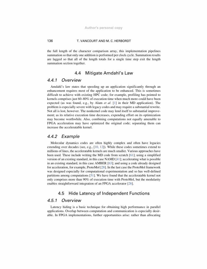
4.5.2 Example
We return to the docking example. There are three independent functions, shown
in Fig. 10: rotation, correlation, and filtering. The correlations must be repeated
at many three-axis rotations: over 104 for typical 10-degree sampling intervals.
Implementations on sequential processors typically rotate the molecule in a step
separate from the correlation.
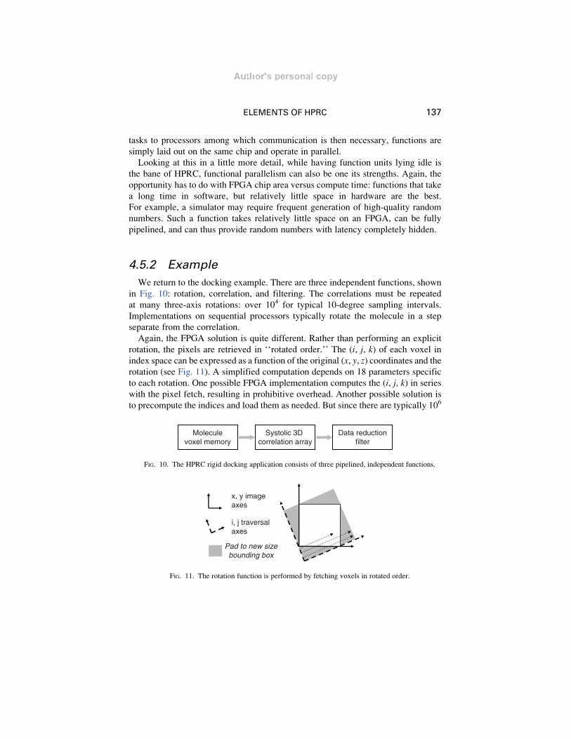
Again, the FPGA solution is quite different. Rather than performing an explicit
rotation, the pixels are retrieved in ‘‘rotated order.’’ The (i, j, k) of each voxel in
index space can be expressed as a function of the original (x, y, z) coordinates and therotation (see Fig. 11). A simplified computation depends on 18 parameters specific
to each rotation. One possible FPGA implementation computes the (i, j, k) in series
with the pixel fetch, resulting in prohibitive overhead. Another possible solution is
to precompute the indices and load them as needed. But since there are typically 106
Data reductionfilter
Moleculevoxel memory
Systolic 3D correlation array
FIG. 10. The HPRC rigid docking application consists of three pipelined, independent functions.
x, y image axes
i, j traversal axes
Pad to new sizebounding box
FIG. 11. The rotation function is performed by fetching voxels in rotated order.
ELEMENTS OF HPRC 137
personal copy
voxels and 104 rotations, this would require gigabytes of storage, and so not lend
itself to rapid retrieval.
The preferred FPGA solution is based on the run-time index calculation, but with
two modifications. The first is that the index calculator be a separate hardware
module; this only requires a few percent area of a contemporary high-end FPGA.
The second is that the calculator be fully pipelined so that the rotation-space
coordinates are generated at operating frequency.
4.6 Speed-Match Sequential Computations
4.6.1 Overview
If a computation pipeline has strictly linear structure, it can run only at the speed
of the slowest element in the pipeline. It is not always convenient or even possible to
insert pipelining registers into a time-consuming operation to increase its clock rate.
Instead, the pipeline element can be replicated to operate in parallel and used in
rotation to get the desired throughput.
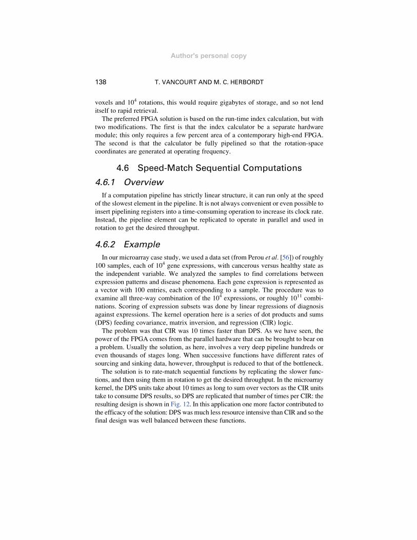
4.6.2 Example
In our microarray case study, we used a data set (from Perou et al. [56]) of roughly100 samples, each of 104 gene expressions, with cancerous versus healthy state as
the independent variable. We analyzed the samples to find correlations between
expression patterns and disease phenomena. Each gene expression is represented as
a vector with 100 entries, each corresponding to a sample. The procedure was to
examine all three-way combination of the 104 expressions, or roughly 1011 combi-
nations. Scoring of expression subsets was done by linear regressions of diagnosis
against expressions. The kernel operation here is a series of dot products and sums
(DPS) feeding covariance, matrix inversion, and regression (CIR) logic.
The problem was that CIR was 10 times faster than DPS. As we have seen, the
power of the FPGA comes from the parallel hardware that can be brought to bear on
a problem. Usually the solution, as here, involves a very deep pipeline hundreds or
even thousands of stages long. When successive functions have different rates of
sourcing and sinking data, however, throughput is reduced to that of the bottleneck.
The solution is to rate-match sequential functions by replicating the slower func-
tions, and then using them in rotation to get the desired throughput. In the microarray
kernel, the DPS units take about 10 times as long to sum over vectors as the CIR units
take to consume DPS results, so DPS are replicated that number of times per CIR: the
resulting design is shown in Fig. 12. In this application one more factor contributed to
the efficacy of the solution: DPS was much less resource intensive than CIR and so the
final design was well balanced between these functions.
138 T. VANCOURT AND M. C. HERBORDT
Author's personal copy
4.7 High Performance = High-Performance
Data Access
4.7.1 Overview
The ‘‘memory wall’’ is often said to limit HPC performance. In tuning applications,
therefore, a great deal of effort goes into maximizing locality through careful place-
ment of data and ordering of data accesses. With FPGAs, our experience is that there
is no one wall; instead, there are many different ones, each characterized by a different
pattern of memory access. Data placement and access orchestration are still critical,
although with a different memory model. An additional opportunity for optimization
results from configuring the multiple internal memory buses to optimize data access
for a particular application.
Already mentioned is that if you can use the full bandwidth at any level of the
memory hierarchy, the application is likely to be highly efficient. Added here is that
on an FPGA, complex parallel memory access patterns can be configured. This
problem was the object of much study in the early days of array processors (see,
e.g., [48]): the objective was to enable parallel conflict-free access to slices of data,
such as array rows or columns, followed by alignment of that data with the correct
processing elements. With the FPGA, the programmable connections allow this
capability to be tailored to the application-specific reference patterns (see, e.g., [70]).
4.7.2 Examples
For our first application, we continue with the microarray analysis case study.
The kernel computation is as before; here we add a communication network to route
triplets of input vectors to the DPS units. The FPGA used has enough computing
Covariance,inverse, andregression
D
D
DD
Dot products and sums
Dot products & sums
Dot products and sums
Result registers
FIG. 12. In the microarray case study, the dot-product bottleneck can be removed by replicating the
slow elements.
ELEMENTS OF HPRC 139
Author's personal copy
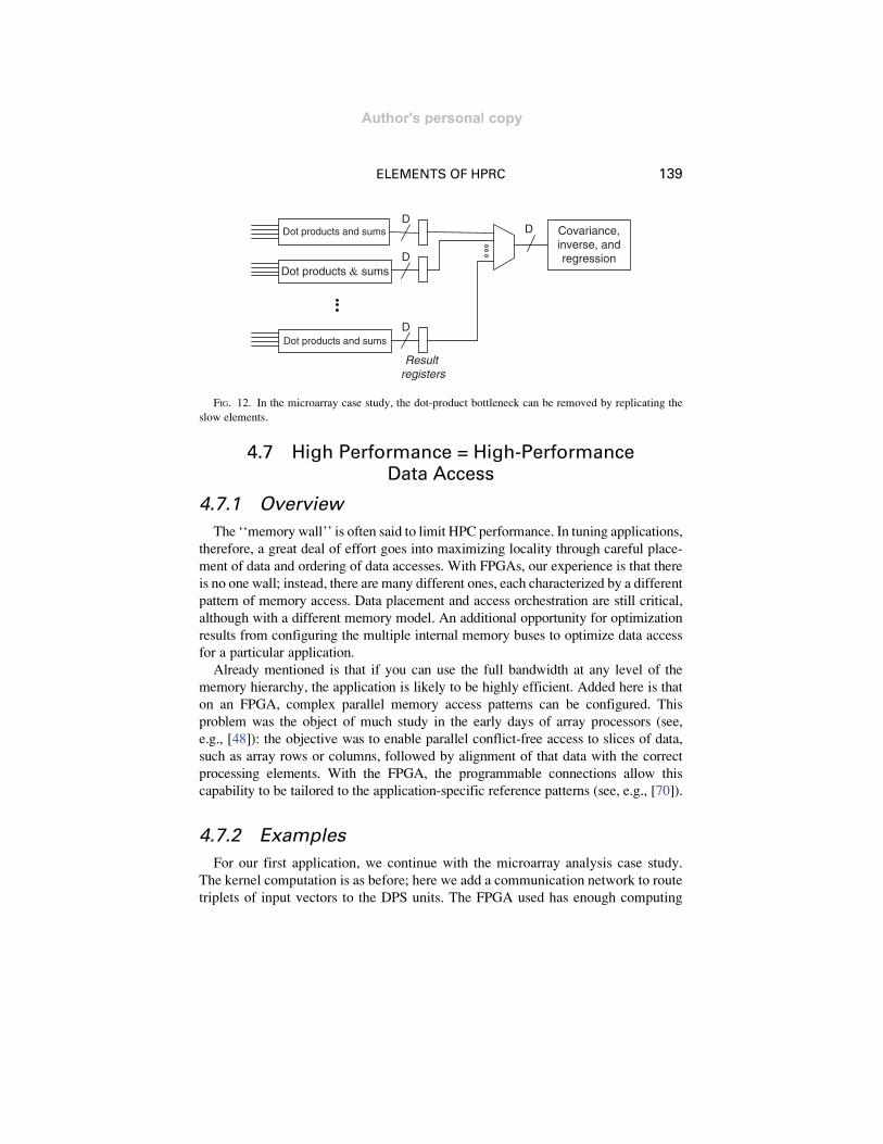
fabric to instantiate 90 DPS pipelines. Each DPS processes three vectors of mea-
surement data (X-vectors) plus one vector of diagnosis values (the Y-vector).Diagnoses are the same in all cases, but each DPS must process a different set of
three X values, or 270 in all. At 4 bits per X value, that would have required over
1000 bits of memory data per cycle.
Although feasible within chip resources, system considerations showed that our
host and backplane would not be able to supply data fast enough to keep the
computation units busy. Instead of accessing 270 values from memory, our imple-
mentation accesses only nine, as shown in Fig. 13. This bus subsets the nine X values
into all possible subsets of size three—84 subsets in all. Although the data bus reads
only nine X values from RAM, the FPGA’s high capacity for fan out turns that into
252 values supplied to computation units, a 28� boost at essentially no hardware cost.
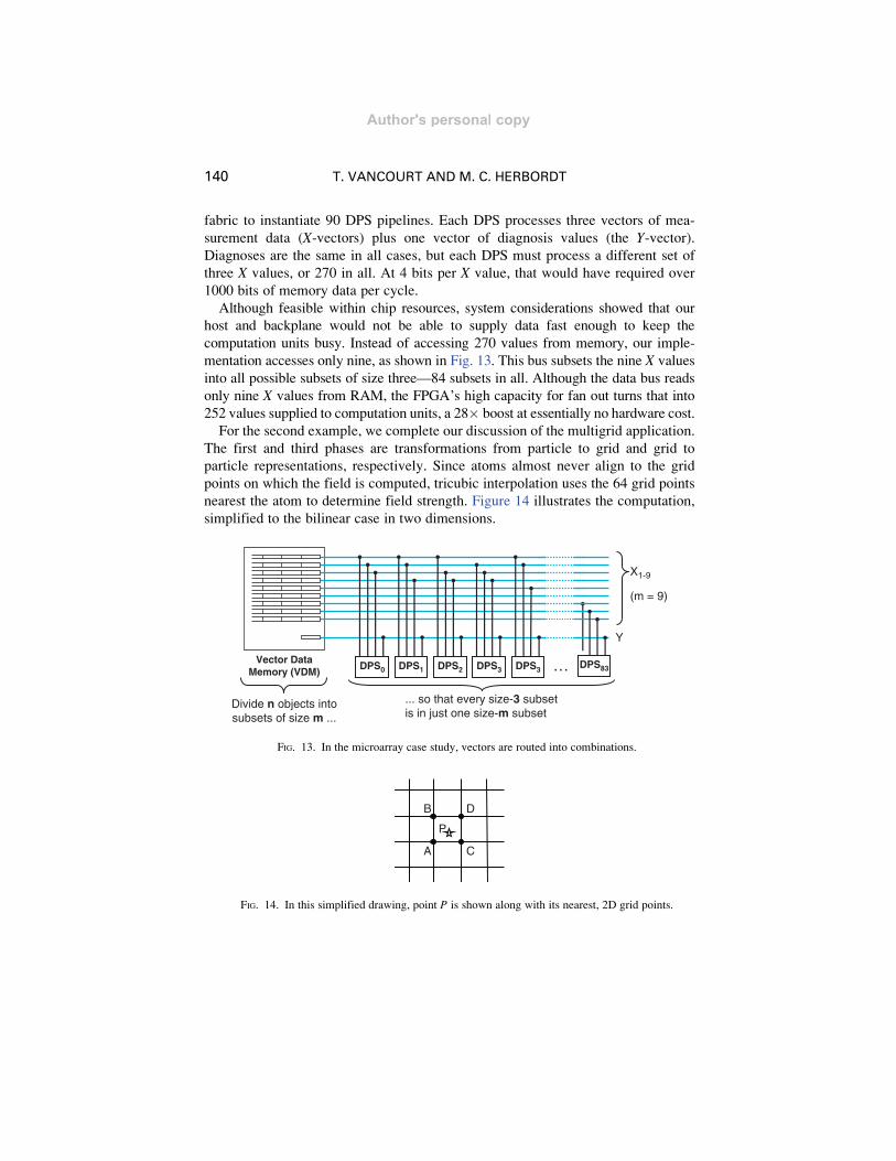
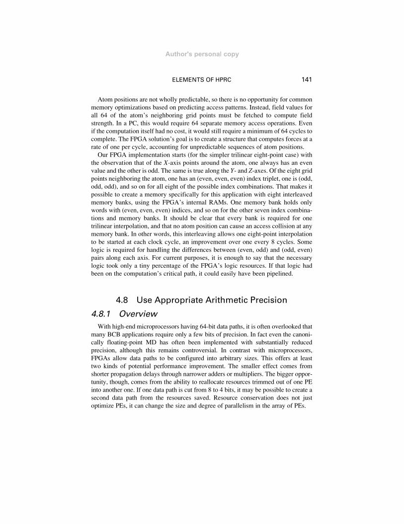
For the second example, we complete our discussion of the multigrid application.
The first and third phases are transformations from particle to grid and grid to
particle representations, respectively. Since atoms almost never align to the grid
points on which the field is computed, tricubic interpolation uses the 64 grid points
nearest the atom to determine field strength. Figure 14 illustrates the computation,
simplified to the bilinear case in two dimensions.
DPS0 DPS1 DPS2 DPS3 DPS3 DPS83…
Y
X1-9
(m = 9)
Vector DataMemory (VDM)
Divide n objects intosubsets of size m ...
... so that every size-3 subsetis in just one size-m subset
FIG. 13. In the microarray case study, vectors are routed into combinations.
A C
P
B D
FIG. 14. In this simplified drawing, point P is shown along with its nearest, 2D grid points.
140 T. VANCOURT AND M. C. HERBORDT
Author's personal copy
Atom positions are not wholly predictable, so there is no opportunity for common
memory optimizations based on predicting access patterns. Instead, field values for
all 64 of the atom’s neighboring grid points must be fetched to compute field
strength. In a PC, this would require 64 separate memory access operations. Even
if the computation itself had no cost, it would still require a minimum of 64 cycles to
complete. The FPGA solution’s goal is to create a structure that computes forces at a
rate of one per cycle, accounting for unpredictable sequences of atom positions.
Our FPGA implementation starts (for the simpler trilinear eight-point case) with
the observation that of the X-axis points around the atom, one always has an even
value and the other is odd. The same is true along the Y- and Z-axes. Of the eight gridpoints neighboring the atom, one has an (even, even, even) index triplet, one is (odd,
odd, odd), and so on for all eight of the possible index combinations. That makes it
possible to create a memory specifically for this application with eight interleaved
memory banks, using the FPGA’s internal RAMs. One memory bank holds only
words with (even, even, even) indices, and so on for the other seven index combina-
tions and memory banks. It should be clear that every bank is required for one
trilinear interpolation, and that no atom position can cause an access collision at any
memory bank. In other words, this interleaving allows one eight-point interpolation
to be started at each clock cycle, an improvement over one every 8 cycles. Some
logic is required for handling the differences between (even, odd) and (odd, even)
pairs along each axis. For current purposes, it is enough to say that the necessary
logic took only a tiny percentage of the FPGA’s logic resources. If that logic had
been on the computation’s critical path, it could easily have been pipelined.
4.8 Use Appropriate Arithmetic Precision
4.8.1 Overview
With high-end microprocessors having 64-bit data paths, it is often overlooked that
many BCB applications require only a few bits of precision. In fact even the canoni-
cally floating-point MD has often been implemented with substantially reduced
precision, although this remains controversial. In contrast with microprocessors,
FPGAs allow data paths to be configured into arbitrary sizes. This offers at least
two kinds of potential performance improvement. The smaller effect comes from
shorter propagation delays through narrower adders or multipliers. The bigger oppor-
tunity, though, comes from the ability to reallocate resources trimmed out of one PE
into another one. If one data path is cut from 8 to 4 bits, it may be possible to create a
second data path from the resources saved. Resource conservation does not just
optimize PEs, it can change the size and degree of parallelism in the array of PEs.
ELEMENTS OF HPRC 141
Author's personal copy

4.8.2 Examples
All applications described here benefit substantially from the selection of non-
standard data type sizes. Microarray values and biological sequences require only
4–5 bits, shape characterization of a rigid molecule only 2–7. While MD probably
requires more than the 24 bits provided by single-precision floating point, double
precision (53 bits) may not be required [27].
The tradeoff between PE complexity and degree of parallelism was made clear in
the docking case study [71]. There we examined six different models describing
intermolecular forces. Molecule descriptions range from 2 to 7 bits per voxel, and
scoring functions varied with the application. Fitting the various maximum-sized
cubical computing arrays into a Xilinx XC2VP70, the number of PEs ranged from
512 to 2744. Since clock speeds also differed for each application-specific accelera-
tor, they covered a 7:1 performance range. If we had been restricted to, say, 8-bit
arithmetic, the performance differential would have been even greater.
Similar, though less dramatic, results appeared in a case study that accelerated the
computation core of the ProtoMol molecular dynamics code [27]. There we pre-
sented a careful examination of computation quality, measured as numerical stabil-
ity, as a function of the number of bits used for computation. We observed that, after
about 35 bits of precision in the accumulators, there was little additional gain in the
quality measure. That allowed eight force pipelines to be instantiated rather than
four. Because of the difficulty in routing the larger design, only a small performance
gain was observed, however.
4.9 Use Appropriate Arithmetic Mode
4.9.1 Overview
Microprocessors provide support for integer and floating point data types, and,
depending on multimedia features, 8-bit saturated values. In digital signal processing
systems, however, cost concerns often requireDSPs to have only integers. Software can
emulate floating point, when required; also common is block floating point. FPGA’s
analogous situation is that, although plausible, single-precision floating point remains
costly and should be avoided if possible, with well-tuned libraries available. Alterna-
tives include the block floating point, log representations, and the semifloating point.
4.9.2 Example
The MD computation’s inner kernel operation requires computing r�14 and r�8
for the radius r between atoms, over a wide range, usually with a table lookup.
We would generally use double-precision floating point for further computations.
142 T. VANCOURT AND M. C. HERBORDT
Author's personal copy
Careful analysis shows that the number of computed distinct alignments is quite
small even though the range of exponents is large. This enables the use of a stripped-
down floating-point mode, particularly one that does not require a variable shift.
The resulting force pipelines (with 35-bit precision) are 25% smaller than ones built
with a commercial single-precision (24-bit) floating-point library.
4.10 Minimize Use of High-Cost Arithmetic
4.10.1 Overview
The relative costs of arithmetic functions are very different on FPGAs than they
are on microprocessors. For example, FPGA integer multiplication is efficient in
comparison with addition, while division is orders of magnitude slower. Even if the
division logic is fully pipelined to hide its latency, the cost is still high in chip area,
especially if the logic must be replicated. On an FPGA, unused functions need not be
implemented; recovered area can then be used to increase parallelism. Thus restruc-
turing arithmetic with respect to an FPGA cost function can result in substantial
performance gain.
A related tradeoff involves the general observation that these differences encour-
age careful attention to the way in which numbers are represented and the ways in
which arithmetic operations are implemented, decisions that often go together.
4.10.2 Example
The microarray data analysis kernel as originally formulated requires division.
Our solution is to represent some numbers as rationals, maintaining separate numer-
ator and denominator, replacing division operations with multiplication. This dou-
bles the number of bits required, but rational values are needed only in a short, late
occurring segment of the data path. As a result, the additional logic needed for the
wider data path is far lower than logic for division would have been.
We also turn to the microarray application for an example of where rewriting
expressions can be helpful. This application originally involved a matrix inversion
for each evaluation.
We initially expressed the problem as a 4 � 4-matrix, which would then need to
be inverted to find the final result. This, however, led to an unacceptable complexity
in the hardware computation. After additional research, we found an equivalent way
to phrase the problem. It required more computation in setting up the problem, and
more bits of precision in the intermediate expressions, but allowed us to reduce the
system to a 3� 3-matrix. The net effect was to reduce overall computing complexity
at the cost of some increase in the number of bits needed in the intermediate results.
ELEMENTS OF HPRC 143
Author's personal copy
At this point, Cramer’s rule became an attractive solution technique. The algorithm
is notoriously unstable, and has polynomial complexity of N! in the size of the matrix.
At this small array size, however, N! is still small enough for the algorithm to be
feasible and it does not have enough terms for the instabilities to accumulate. We also
knew that the matrix (and therefore its inverse) was symmetric, so some result terms
could be copied rather than recomputed. As a result, the inverse could be expressed in
closed form using a manageable number of terms. Since we knew that the input values
had only 4-bit precision, we were able to reduce the precision of some intermediate
expressions—4-bit input precision hardly justifies 64-bit output precision.
4.11 Support Families of Applications Rather
Than Point Solutions
4.11.1 Overview
HPC applications are often complex and highly parameterized: this results in the
software having variations not only in data format, but also in algorithm to be
applied. These variations, including parameterization of functions, are easily sup-
ported with contemporary object-oriented technology. This level of parameteriza-
tion is far more difficult to use in current HDLs, but enables higher reuse of the
design. Amortization of development cost is over a larger number of uses, and there
is less reliance on skilled hardware developers for each variation on the application.
4.11.2 Example
Essential methods for searching biological databases are based on dynamic
programming (DP). Although generally referred to by the name of one variation,
Smith–Waterman, DP-based approximate string matching is a large number of related
algorithms, which vary significantly in purpose and complexity. Achieving high
performance in HPRC requires careful tuning to the specifics of the application,
which limits a component’s reusability. General, programmable PEs rarely approach
the speed or resource efficiency of tuned applications. Reusable HPC/FPGA applica-
tions must resolve the conflicting requirements of generality and customization.
We start with two observations on component reuse in FPGA systems. The first is
that, in traditional hardware design systems, components are black boxes with
limited parameterization of their internals. Reuse consists largely of creating com-
munication and synchronization structures between them, and connecting them to
the memory subsystems. The second observation is that, in HPRC, it is often the
leaf data types and arithmetic expressions that change between applications, that is,
the innermost components. The FPGA system’s performance depends on its
144 T. VANCOURT AND M. C. HERBORDT
Author's personal copy
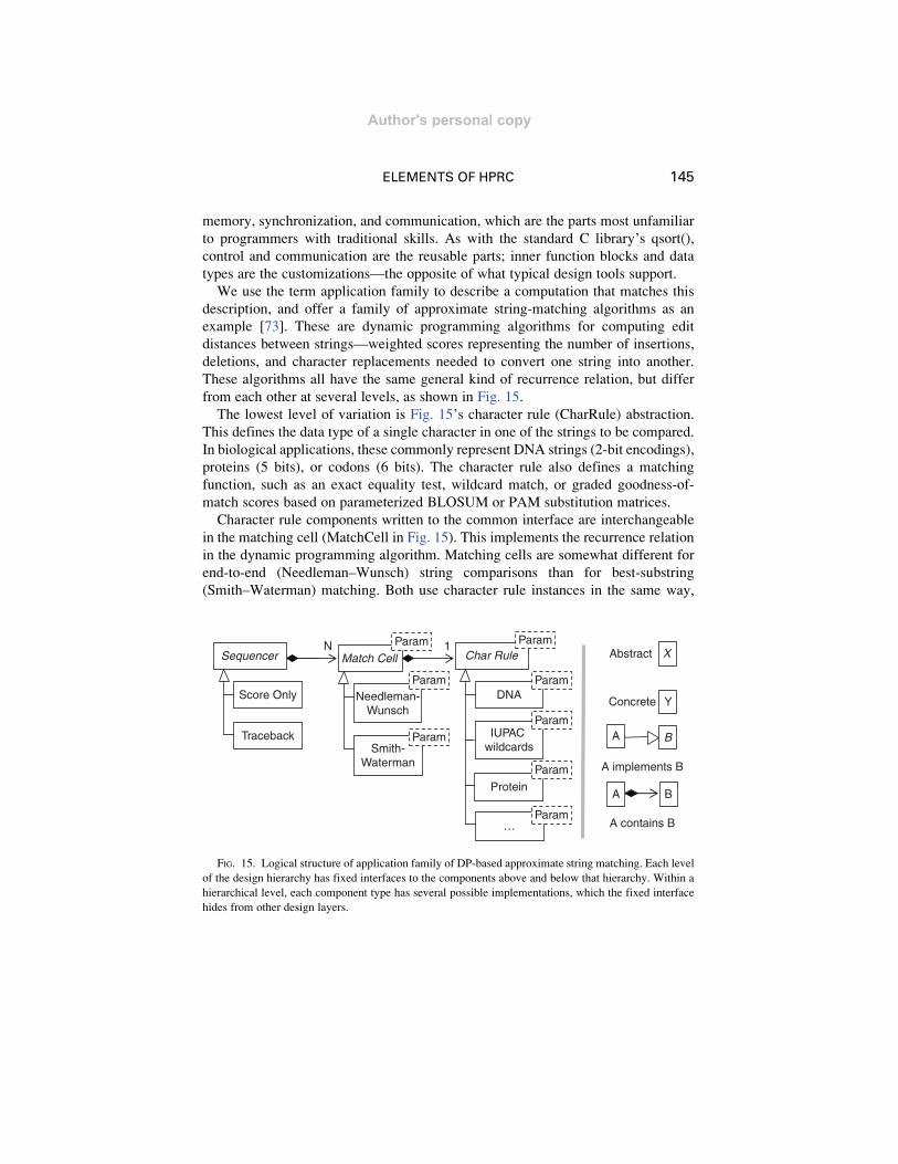
memory, synchronization, and communication, which are the parts most unfamiliar
to programmers with traditional skills. As with the standard C library’s qsort(),
control and communication are the reusable parts; inner function blocks and data
types are the customizations—the opposite of what typical design tools support.
We use the term application family to describe a computation that matches this
description, and offer a family of approximate string-matching algorithms as an
example [73]. These are dynamic programming algorithms for computing edit
distances between strings—weighted scores representing the number of insertions,
deletions, and character replacements needed to convert one string into another.
These algorithms all have the same general kind of recurrence relation, but differ
from each other at several levels, as shown in Fig. 15.
The lowest level of variation is Fig. 15’s character rule (CharRule) abstraction.
This defines the data type of a single character in one of the strings to be compared.
In biological applications, these commonly represent DNA strings (2-bit encodings),
proteins (5 bits), or codons (6 bits). The character rule also defines a matching
function, such as an exact equality test, wildcard match, or graded goodness-of-
match scores based on parameterized BLOSUM or PAM substitution matrices.
Character rule components written to the common interface are interchangeable
in the matching cell (MatchCell in Fig. 15). This implements the recurrence relation
in the dynamic programming algorithm. Matching cells are somewhat different for
end-to-end (Needleman–Wunsch) string comparisons than for best-substring
(Smith–Waterman) matching. Both use character rule instances in the same way,
Abstract
Concrete
A implements B
A contains B
Y
B
A
Score Only
Traceback
Needleman-Wunsch
Smith-Waterman
DNA
IUPAC wildcards
Protein
…
N Param Param
Param
Param
Param
Param
Param
Param
A
1Sequencer Match Cell Char Rule X
B
FIG. 15. Logical structure of application family of DP-based approximate string matching. Each level
of the design hierarchy has fixed interfaces to the components above and below that hierarchy. Within a
hierarchical level, each component type has several possible implementations, which the fixed interface
hides from other design layers.
ELEMENTS OF HPRC 145
Author's personal copy

and assume the same communication paths between matching cells. The similarities
are captured in their shared abstraction; their differences in algorithm and in
bookkeeping data are hidden in their private implementation details.
At the third level, data are sequenced through the matching cells in one of two
ways: in a single matching pass, producing only an integer similarity score, or with a
second traceback pass that records the character by character relationships that yield
the highest score.
Our initial implementation using the LAMP tool suite [68, 69] allowed over 200
combinations of the three component types, with many more variations possible
through parameter settings. This structure was quite natural in the object-oriented
algorithms we used but required more configurability than VHDL features provide.
4.12 Scale Application for Maximal Use of
Target Hardware
FPGA-based computations very often differ from standard logic applications in one
critical feature. Logic designs typically have specific performance goals. Success is
binary: a design does or does not meet its timing requirements. There is little or no
benefit in exceeding requirements by a larger margin. In computing applications,
however, faster is better. Since computation accelerators are very often arrays of PEs,
and since performance is typically dominated by the degree of parallelism, part of
accelerator design consists of instantiating as many PEs as the FPGA’s computing
fabric will support. The number of PEs depends on three sources of information: the
FPGA’s capacity, the geometry of the array defined by the application family, and
the sizes of PEs defined by a specific member of the application family [72].
FPGA capacity has several terms, according to the hardware resources available:
hard multipliers and block RAMs as well as general-purpose logic elements. Even at
that, capacity is hard to abstract across different families of FPGAs. For example,
block RAMs in Xilinx Virtex-II FPGAs are 18 Kbit units, but Altera’s Stratix family
offers a combination of 512-bit, 4 Kbit, and 512 Kbit units. The Altera FPGA family
that corresponds most closely to V5 is Stratix IV. In that family, the Ram sizes are
640 b, 9k b, 144k b. Multiple units can be combined, in both systems, to create a
wide variety of logical memory structures, but the Virtex and Stratix resources are
not interchangeable in all cases.
The application family defines the geometry of the computation array. As shown
in Fig. 16A, arrays can be simple linear structures. Other geometries are possible,
however, and present different problems for designers optimizing the performance
of computing arrays. Figure 16B illustrates a rectangular array. It is characterized by
two different architectural parameters (N1 for height and N2 for width) rather than
just one. Architectural parameters need not be numbers of PEs; they can abstract
146 T. VANCOURT AND M. C. HERBORDT
Author's personal copy

aspects of the design in arbitrary ways. They can also introduce new kinds of
constraints, for example, when a rectangular array requires width greater than or
equal to its height.
Figure 16D illustrates a tree-structured computing array, showing just one of the
ways that arrays can grow according to exponential or other nonlinear law. We have
also observed computing arrays like, that in Fig. 16C, composed of multiple coupled
subsystems. In many cases, the different subsystems grow according to different
algebraic growth laws, at the same time that they remain coupled to each other.
Because different subsystems often use different FPGA resources (as in Fig. 16E),
either resource can be the one that limits eventual growth of the computing array.
Of course, computing arrays can combine these features. The growth law can include
multiple architectural parameters, nonlinear growth patterns, coupled subsystems that
grow according to different algebraic laws, and use of multiple resource types.
The form of the computing array is defined by the application family, but the size
of each PE in the array depends on the specific member of the application family.
In string applications, PE size depends on the number of bits in the string element
(e.g., 2 bits for DNA or 5 bits for proteins) and on the kinds of comparison being
performed. In the drug-docking application, PE size depends on the number of bits per
voxel and on the function used to score juxtaposition of the two voxel values.
In this view, the size of an FPGA-based computing array is not a design parameter
but a natural result of other design features. The array’s architectural parameters are
N
Linear array.one structural
parameter N2B: Rectangular array.
N1 � N2 PEs
N1
N
Tree of depth N.2N−1 PEs
N
C: Coupled structures.related sizes N, N2, N3
Logic
E: Multiple FPGA resources,with dependencies between
allocation amounts
RAM
A
D
B C
FIG. 16. Growth force laws for computing arrays specified in terms of architectural parameters.
(A) Linear array—one structural parameter. (B) Rectangular array—N1 � N2 PEs. (C) Coupled
structures—related sizes N, N2, N3. (D) Tree of depth N � 2N � 1 PEs. (E) Multiple FPGA resources,
with dependencies between allocation amounts.
ELEMENTS OF HPRC 147
Author's personal copy
chosen to maximize some application-specific function that represents the value of
different configurations. The ‘‘best’’ architectural parameter values are the ones that
define the array of highest value, as long as the array’s structure is valid for that
application family, and as along as the family member’s PEs live within the FPGA’s
resource budget. Automating this kind of optimization is possible within the experi-
mental LAMP design system [68, 69, 72]; it cannot be expressed in mainstream
design automation tools or methodologies.
5. GPGPU An Alternative Approach toAcceleration
5.1 Overview
Graphics processing units (GPUs), such as those from Nvidia and ATI/AMD,
present another emerging technology in HPC. By intent, GPUs address the seem-
ingly insatiable need for graphics performance in gaming—a market of millions of
units annually. Because their architecture optimizes a few basic features of real-time
graphics computing, they offer a huge performance boost over standard processors
for typical graphics applications. First, the rendering pipeline has a fixed, widely
accepted structure, so the processing pipeline can be tuned to that sequence of
operations. Second, pixels in different parts of a scene tend to have few dependen-
cies between them, allowing them to be computed independently of pixels elsewhere
in the image. Third, pixels close to each other, for example, on the same side of some
geometric figure, can often be processed using the same set of operations on slightly
different pixel values, allowing a high degree of SIMD parallelism.
Despite the relatively specialized goals of GPUs, their programming model has
been adapted for a wide range of applications. As with HPRC, successful accelera-
tion depends on aligning the implementation to the assumptions built into the
underlying hardware. Although recent generations of GPUs have additional features
that support general programming with GPUs (GPGPU), the features that both
enable and limit performance have remained constant. These fall into several
major categories, including:
l Data path structure
l Memory access
l Scheduling of processing tasks
Although somewhat intertwined, these need to be considered individually, and in
contrast to FPGA programming.
148 T. VANCOURT AND M. C. HERBORDT
Author's personal copy

5.2 Data Path Structure
Figure 17 illustrates the logical structure of GPU acceleration hardware. There
has been rapid advancement in years. The biggest changes, however, have been in
capacity, rather than in drastic architectural updates.
Pixel processing operations have traditionally been characterized by arithmetic
intensity (including floating point, 2D interpolations, exponents, and trigonometry
operations), but simple control structures and short code fragments. Although
capacities keep improving, the code fragments (sometimes called ‘‘shaders’’
because of their graphics heritage) have been strictly limited in length. Early
GPUs allowed only as few as 64 assembly-level operations. Sizes of code buffers
have increased, however, and virtualization allows effectively unlimited numbers of
instructions—but with a high penalty when the hardware’s code buffer size is
exceeded.
Early GPUs used a strict SIMDmodel, performing the same calculation on a large
set of pixels. This made conditional logic difficult, when possible at all, because all
of the SIMD PEs would have to execute both the ‘‘then’’ and ‘‘else’’ branches of a
conditional, selectively quashing results from one branch or the other according to
each PE’s condition settings. More recent GPUs allow greater flexibility in condi-
tional execution, including looping constructs, but good GPU performance often
argues against using these features.
Tasks awaiting inputand task scheduler
SIMDArithmetic
units
Output waiting to be writtenand output scheduler
Maingraphicsmemory(off chip)
FIG. 17. Logical structure of a GPU.
ELEMENTS OF HPRC 149
Author's personal copy

Although the arithmetic units in a GPU have fixed structure, there is some
flexibility in scratch storage. A fixed amount of space for holding the PEs’ operands
exists, but it can be partitioned differently across the whole ensemble of PEs. Of
course, larger allocations to some PEs mean smaller allocations to others, possibly
preventing those other PEs from being used at all.
Also, the GPU supports little to no communication between PEs. Recent genera-
tions allow some sharing of data between PEs via on-chip buffers, but the main
memory remains the only way to exchange large amounts of data between peer PEs
or between successive stages of a processing pipeline. As we describe in the next
sections, this represents a challenge in exploiting the GPU’s processing power.
5.3 Memory Access
The GPU has some amount of on-chip scratch memory that can be accessed by
many PEs concurrently, and often has modest memory resources of other kinds. Bulk
data storage, however, relies entirely on the GPU’s on-board memory. GPUs typically
cannot access host memory on their own; the CPU must initiate all data transfers. As a
result, even on-board memories of 1 GB or more can become a limiting resource when
shared among input data, output data, and intermediate results.
GPU memory is famous for raw bandwidth. Some current models transfer 320 or
more bits per clock cycle at rates over 1.5 GHz. Used properly, a GPU can sustain
impressive data transfer bandwidth to and from the on-board RAM. This model
presents two obvious constraints, however. First, the pipelining in the memory itself,
plus additional delays into and out of the GPU, can result in latencies of tens of
memory cycles. To sustain throughput, the GPU must have enough tasks available
so that many of them can wait for input or output while others occupy the SIMD
processors. Second, wide transfers necessarily carry many data words at each
memory cycle. Bandwidth is wasted if some of those words are not used.
These features of the GPU memory hierarchy have potentially substantial impli-
cations for the application programmer: poor use results in order-of-magnitude
performance loss. Wide accesses mean that sparse data structures (like C structs in
which not all elements are used) waste bandwidth. Long latency combined with
limited communication paths between PEs penalize data dependencies, beyond
those within a single code fragment. Also, subtle effects arise, for example, when
computing a vector sum ‘‘x ¼ a + b’’ on operands aligned differently.
5.4 Task Scheduling
At first glance, the programming model might seem daunting. It requires
hundreds to thousands of concurrent tasks to use the hardware effectively, since
large numbers of tasks must wait for operands to load from memory or results to
150 T. VANCOURT AND M. C. HERBORDT
Author's personal copy

store into memory at any given time. Then, memory reads and writes must be
scheduled to maximize the utilization of different operands or result slots within
each memory transfer. If scheduling needed to be done by the application program-
mer, for example, by using common system primitives, then this task would be
infeasible for all but a very few skilled programmers.
Instead, GPUs move scheduling responsibilities into hardware. In some ways, this
resembles data flow computing. As a task (or SIMD task group) has all its depen-
dencies met, it moves to the arithmetic units. On the other side, and somewhat
symmetric to the input operations, some number of completed tasks awaits retire-
ment of results into main memory. Here, the scheduler’s job is to bundle results from
different tasks into a single memory transfer, so that the largest possible number of
16- or 32-bit words in a transfer carry payload data.
An application developer must understand at least this much about the GPU’s task
scheduler to use the GPU’s parallelism effectively. It is not enough to keep all of the
PEs busy. The programmer must create a large factor more threads than PEs so that
not only are those used, but so that tasks waiting to load operands or store results can
use the whole width of each memory transfer effectively. A GPU’s potential
performance is rarely realized until the application makes hundreds or thousands
of tasks available to the scheduler.
Since GPU computations work best as sequences of relatively small computa-
tions, a second level of scheduling also becomes important. The host CPU must
synchronize and schedule macroevents, such as major phases of execution, while the
GPU itself schedules microevents, such as fetching of operands or selection
of individual tasks to run. Starting and flushing the GPU’s execution pipeline
represents more potential loss of efficiency.
5.5 Comparison with HPRC
Although broad generalizations always have exception, a few basic factors tend to
distinguish FPGA-based from GPU-based computing. These include:
l Fixed versus configurable data path. GPUs use ASIC optimizations to tune
performance for data types and operations supported. While FPGAs also have
ASIC optimizations, these are at a lower level. FPGAs thus allow arbitrary data
types and operations, enabling detailed tradeoffs between numbers of bits per
operation and numbers of hardware operators instantiated.
l Fixed versus configurable memory structure. GPUs achieve high potential
bandwidth using memory and cache structures optimized for rendering opera-
tions. FPGAs offer flexibility in the number and width of off-chip memories,
ELEMENTS OF HPRC 151
Author's personal copy
and in arrangement of their hundreds to thousands of independently addressable
on-chip RAM blocks.
l Organization of parallelism. GPUs offer a fixed parallelism model built around
SIMD processing and limited dependencies among data elements. FPGAs
allow arbitrary combinations of pipelined and broadside parallelism, and can
handle complex communication among processing elements.
l Familiarity of programming model. In GPUs, operations on individual data
elements can be programmed in languages close to familiar C or assembler.
Efficient use of FPGAs usually requires unfamiliar languages, like Verilog or
VHDL.
l Host communication. GPUs have limited kinds of interactions with host mem-
ory. Different FPGA accelerators have different host interaction capabilities.
For example, direct Hypertransport connection offers the possibility of access
to all of host memory under FPGA control.
l Floating-point support. GPUs have traditionally had better floating-point sup-
port, up to the set of hardware primitives supported. Larger FPGAs and recent
tool innovations [47] have reduced their performance differences.
Each does well at a specific class of operations. If you can cast your application
into the GPU’s computing model and create enough parallelism (hundreds- to
thousands-way), GPUs can do very well, and with widely accessible programming
skills. FPGAs do better with idiosyncratic control, data types, concurrency models,
and degrees of parallelism. Even with the complexities of GPU memory optimiza-
tion, FPGAs often require unfamiliar programming skills to reach their performance
potential.
6. Conclusion
FPGA-based computation is just now emerging into the main stream of comput-
ing practice. Practitioners do not yet have the experience, programming idioms, and
tool support needed for pushing FPGAs to their performance potential, and experi-
ence from the logic design community has limited value for HPC application. Good
tool support will come from a good understanding of the general principles and
techniques of FPGA-based computation. General principles can only come from
experience with real applications.
We present our case studies, with the lessons learned from them, as a step toward
wider use of FPGAs in HPC. Those lessons include intangible advice to application
designers. Other lessons have enabled construction of specific design tools,
152 T. VANCOURT AND M. C. HERBORDT
Author's personal copy
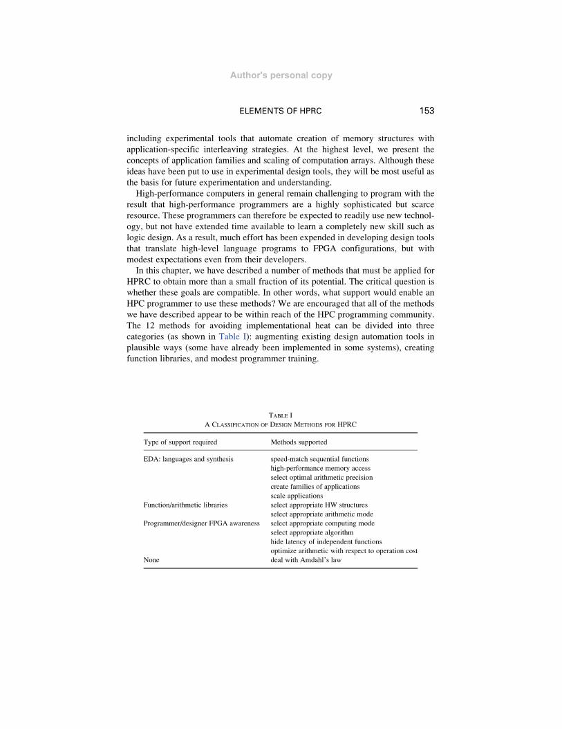
including experimental tools that automate creation of memory structures with
application-specific interleaving strategies. At the highest level, we present the
concepts of application families and scaling of computation arrays. Although these
ideas have been put to use in experimental design tools, they will be most useful as
the basis for future experimentation and understanding.
High-performance computers in general remain challenging to program with the
result that high-performance programmers are a highly sophisticated but scarce
resource. These programmers can therefore be expected to readily use new technol-
ogy, but not have extended time available to learn a completely new skill such as
logic design. As a result, much effort has been expended in developing design tools
that translate high-level language programs to FPGA configurations, but with
modest expectations even from their developers.
In this chapter, we have described a number of methods that must be applied for
HPRC to obtain more than a small fraction of its potential. The critical question is
whether these goals are compatible. In other words, what support would enable an
HPC programmer to use these methods? We are encouraged that all of the methods
we have described appear to be within reach of the HPC programming community.
The 12 methods for avoiding implementational heat can be divided into three
categories (as shown in Table I): augmenting existing design automation tools in
plausible ways (some have already been implemented in some systems), creating
function libraries, and modest programmer training.
Table I
A CLASSIFICATION OF DESIGN METHODS FOR HPRC
Type of support required Methods supported
EDA: languages and synthesis speed-match sequential functions
high-performance memory access
select optimal arithmetic precision
create families of applications
scale applications
Function/arithmetic libraries select appropriate HW structures
select appropriate arithmetic mode
Programmer/designer FPGA awareness select appropriate computing mode
select appropriate algorithm
hide latency of independent functions
optimize arithmetic with respect to operation cost
None deal with Amdahl’s law
ELEMENTS OF HPRC 153
Author's personal copy
Acknowledgments
This work was supported in part by the NIH through awards #R01 RR023168-01 and #R21 RR020209-01
by an IBM Faculty Award, and facilitated by donations fromAltera Corporation, Xilinx Corporation, SGI,
and XtremeData, Inc.
References
[1] Alam S., Agarwal P., Smith M., Vetter J., and Caliga D., 2007. Using FPGA devices to accelerate
biomolecular simulations. Computer, 40(3): 66–73.[2] Altschul S., Gish W., Miller W., Myers E., and Lipman D., 1990. Basic local alignment search tool.
Journal of Molecular Biology, 215, 403–410.
[3] Azizi N., Kuon I., Egier A., Darabiha A., and Chow P., 2004. Reconfigurable molecular dynamics
simulator. In Proceedings of the IEEE Symposium on Field Programmable Custom ComputingMachines, pp. 197–206.
[4] Baldi P., and Hatfield G., 2002. DNA Microarrays and Gene Expression. Cambridge University
Press, Cambridge, UK.
[5] Benson G., 1999. Tandem repeats finder: A program to analyze DNA sequences. Nucleic AcidsResearch, 27(2): 573–580.
[6] Bhatt A., 2007. Accelerating with many-cores and special purpose hardware. Keynote Talk, Field
Programmable Logic and Applications.
[7] Bluethgen H.-M., and Noll T., 2000. A programmable processor for approximate string matching
with high throughput rate. In Proceedings of ASAP, pp. 309–316.
[8] Borah M., Bajwa R., Hannenhalli S., and Irwin M., 1994. A SIMD solution to the sequence
comparison problem on the MGAP. In Proceedings of ASAP, pp. 336–345.[9] Briggs E., Sullivan D., and Bernholc J., 1996. Real-space multigrid-based approach to large-scale
electronic structure calculations. Physical Review B, 54, 14362–14375.
[10] Brooks B., Bruccoleri R., Olafson B., States D., Swaminathan S., and Karplus M., 1983. Charmm:
Program for macromolecular energy, minimization, and dynamics calculations. Journal ofComputational Chemistry, 4, 187–217.
[11] Buell D., July 2006. Reconfigurable systems. Keynote Talk, Reconfigurable Systems Summer
Institute.
[12] Case D., Cheatham T., III, Darden T., Gohlke H., Luo R., Merz K., Jr., Onufriev A., Simmerling C.,
Wang B., and Woods R., 2005. The Amber biomolecular simulation programs. Journal of Compu-
tational Chemistry, 26, 1668–1688.
[13] Chang C., 2004. BLAST Implementation on BEE2. Electrical Engineering and Computer Science.
University of California, Berkeley.
[14] Chow E., Hunkapiller T., and Peterson J., 1991. Biological information signal processor.
In Proceedings of the International Conference on Application Specific Systems, Architectures,
and Processors, pp. 144–160.[15] Conti A., VanCourt T., and Herbordt M., 2004. Flexible FPGA acceleration of dynamic program-
ming string processing. In Proceedings of the IEEE Conference on Field Programmable Logic and
Applications.[16] Culler D., Singh J., and Gupta A., 1999. Parallel Computer Architecture: A Hardware/Software
Approach. Morgan-Kaufmann, San Francisco, CA.
154 T. VANCOURT AND M. C. HERBORDT
Author's personal copy

[17] D’Amour M., 2008. Reconfigurable computing for acceleration in HPC. FPGA and Structured ASICJournal. http://www.fpgajournal.com/articles_2008/20080226_drc.htm.
[18] DeHon A., Adams J., DeLorimier M., Kapre N., Matsuda Y., Naeimi H., Vanier M., and
Wrighton M., 2004. Design patterns for reconfigurable computing. In Proceedings of the IEEE
Symposium on Field Programmable Custom Computing Machines, pp. 13–23.[19] Ding F., and Dokholyan N., 2005. Simple but predictive protein models. Trends in Biotechnology,
3(9): 450–455.
[20] Dokholyan N., 2006. Studies of folding and misfolding using simplified models. Current Opinion in
Structural Biology, 16, 79–85.[21] Dongarra J., et al., 2008. DARPA’s HPCS program: History, models, tools, languages. In Advances
in Computers, v72: High Performance Computing, M. Zelkowitz, ed. pp. 3–102. Academic Press,
London.
[22] Durbin R., Eddy S., Krogh A., and Mitchison G., 1998. Biological Sequence Analysis. Cambridge
University Press, Cambridge, UK.
[23] Dydel S., andBala P., 2004. Large scale protein sequence alignment using FPGA reprogrammable logic
devices. In Proceedings of the IEEE Conference on Field Programmable Logic and Applications.[24] Ginsberg M., 2008. Bibliographic snapshots of high performance/high productivity computing.
In Advances in Computers, v72: High Performance Computing, M. Zelkowitz, ed. Academic
Press, London.
[25] Gokhale M., Rickett C., Tripp J., Hsu C., and Scrofano R., 2006. Promises and pitfalls of reconfigur-
able supercomputing. In Proceedings of the 2006 Conference on the Engineering of Reconfigurable
Systems and Algorithms, pp. 11–20.
[26] Gu Y., and Herbordt M., 2007. FPGA-based multigrid computations for molecular dynamics
simulations. In Proceedings of the IEEE Symposium on Field Programmable Custom ComputingMachines, pp. 117–126.
[27] Gu Y., VanCourt T., and Herbordt M., 2006. Improved interpolation and system integration for
FPGA-based molecular dynamics simulations. In Proceedings of the IEEE Conference on FieldProgrammable Logic and Applications, pp. 21–28.
[28] Gu Y., VanCourt T., and Herbordt M., 2008. Explicit design of FPGA-based coprocessors for short-
range force computation in molecular dynamics simulations. Parallel Computing, 34(4–5): 261–271.
[29] Guccione S., and Keller E., 2002. Gene matching using JBits. In Proceedings of the IEEEConference on Field Programmable Logic and Applications, pp. 1168–1171.
[30] Gusfield D., 1997. Algorithms on Strings, Trees, and Sequences: Computer Science and
Computational Biology. Cambridge University Press, Cambridge, UK.
[31] Haile J., 1997. Molecular Dynamics Simulation. Wiley, New York, NY.
[32] Herbordt M., Model J., Sukhwani B., Gu Y., and VanCourt T., 2007. Single pass streaming BLAST
on FPGAs. Parallel Computing, 33(10–11): 741–756.
[33] Herbordt M., Gu Y., VanCourt T., Model J., Sukhwani B., and Chiu M., 2008. Computing models
for FPGA-based accelerators with case studies in molecular modeling. Computing in Science &Engineering, 10(6): 35–45.
[34] Herbordt M., Kosie F., and Model J., 2008. An efficient O(1) priority queue for large FPGA-based
discrete event simulations of molecular dynamics. In Proceedings of the IEEE Symposium on FieldProgrammable Custom Computing Machines.
[35] Hoang D., 1993. Searching genetic databases on SPLASH 2. In Proceedings of FCCM, pp. 185–191.
[36] Holland B., Vacas M., Aggarwal V., DeVille R., Troxel I., and George A., 2005. Survey of C-based
application mapping tools for reconfigurable computing. In Proceedings of the 8th InternationalConference on Military and Aerospace Programmable Logic Devices.
ELEMENTS OF HPRC 155
Author's personal copy

[37] Izaguirre J., Hampton S., and Matthey T., 2005. Parallel multigrid summation for the n-bodyproblem. Journal of Parallel and Distributed Computing, 65, 949–962.
[38] Jacob A., Lancaster J., Buhler J., and Chamberlain R., 2007. FPGA-accelerated seed generation in
mercury BLASTP. In Proceedings of the IEEE Symposium on Field Programmable Custom
Computing Machines.[39] Katchalski-Katzir E., Shariv I., Eisenstein M., Friesem A., Aflalo C., and Vakser I., 1992. Molecular
surface recognition: Determination of geometric fit between proteins and their ligands by correlation
techniques. Proceedings of the National Academy of Sciences of the United States of America, 89,
2195–2199.
[40] Kim Y., Noh M.-J., Han T.-D., Kim S.-D., and Yang S.-B., 2001. Finding genes for cancer
classification: Many genes and small number of samples. 2nd. In Annual Houston Forum on Cancer
Genomics and Informatics.
[41] Kindratenko V., and Pointer D., 2006. A case study in porting a production scientific supercomput-
ing application to a reconfigurable computer. In Proceedings of the IEEE Symposium on Field
Programmable Custom Computing Machines, pp. 13–22.
[42] Kitchen D., Decornez H., Furr J., and Bajorath J., 2004. Docking and scoring in virtual screening for
drug discovery: Methods and applications. Nature Reviews. Drug Discovery, 3, 935–949.
[43] Kohane I., Kho A., and Butte A., 2003. Microarrays for an Integrative Genomics. MIT Press,
Cambridge, MA.
[44] Korf I., Yandell M., and Bedell J., 2003. BLAST: An Essential Guide to the Basic Local Alignment
Search Tool. O’Reilly & Associates, Sebastopol, CA.
[45] Krishnamurthy P., Buhler J., Chamberlain R., Franklin M., Gyang K., and Lancaster J., 2004.
Biosequence similarity search on the Mercury system. In Proceedings of the International Confer-
ence on Application Specific Systems, Architectures, and Processors, pp. 365–375.[46] Landau G., Schmidt J., and Sokol D., 2001. An algorithm for approximate tandem repeats. Journal
of Computational Biology, 8(1): 1–18.
[47] Langhammer M., 2008. Floating point data path synthesis for FPGAs. In Proceedings of the IEEEConference on Field Programmable Logic and Applications, pp. 355–360.
[48] Lawrie D., 1975. Access and alignment of data in an array processor. IEEE Transactions on
Computers, C-24(12): 1145–1155.
[49] Liptov R., and Lopresti D., 1986. Comparing long strings on a short systolic array. In SystolicArrays, W. Moore, A. McCabe, and R. Uquhart, Eds. Adam Hilger, Boston, MA.
[50] Lopresti D., 1987. P-NAC: A systolic array for comparing nucleic acid sequences. IEEE Computer,
20(7): 98–99.
[51] Matthey T., 2004. ProtoMol, an object-oriented framework for prototyping novel algorithms for
molecular dynamics. ACM Transactions on Mathematical Software, 30(3): 237–265.
[52] McCallum I., 2007. Platform-Level Services for Accelerators: Intel QuickAssist Technology Accel-
erator Abstraction Layer (AAL). Intel Corporation, Santa Clara, CA.
[53] Model J., and Herbordt M., 2007. Discrete event simulation of molecular dynamics with configur-
able logic. In Proceedings of the IEEE Conference on Field Programmable Logic and Applications,
pp. 151–158. http://www.fpgajournal.com/articles_2007/20070710_cots.htm.
[54] Morris K., 2007. COTS supercomputing. FPGA and Structured ASIC Journal. http://www.
fpgajournal.com/articles_2007/20070710_cots.htm.
[55] Muriki K., Underwood K., and Sass R., 2005. RC-BLAST: Towards an open source hardware
implementation. In Proceedings of the International Workshop on High Performance Computa-
tional Biology.[56] Perou C., et al., 2003. Prediction of clinical outcome with microarray data: A partial least squares
discriminant analysis (PLS-DA) approach. Human Genetics, 112, 581–592.
156 T. VANCOURT AND M. C. HERBORDT
Author's personal copy

[57] Pournara I., Bouganis S.-S., and Constantinides G., 2005. FPGA-accelerated Bayesian learning for
reconstruction of gene regulatory networks. In Proceedings of the IEEE Conference on Field
Programmable Logic and Applications.
[58] Rapaport D., 2004. The Art of Molecular Dynamics Simulation. Cambridge University Press,
Cambridge, UK.
[59] Roberts L., 1989. New chip may speed genome analysis. Science, 244(4905): 655–656.
[60] Sagui C., and Darden T., 2001. Multigrid methods for classical molecular dynamics simulations of
biomolecules. Journal of Chemical Physics, 114, 6578–6591.
[61] Scrofano R., Gokhale M., Trouw F., and Prasanna V., 2006. A hardware/software approach to
molecular dynamics on reconfigurable computers. In Proceedings of the IEEE Symposium on Field
Programmable Custom Computing Machines, pp. 23–32.
[62] Skeel R., Tezcan I., and Hardy D., 2002. Multiple grid methods for classical molecular dynamics.
Journal of Computational Chemistry, 23, 673–684.[63] Smith M., Alam S., Agarwal P., Vetter J., and Caliga D., 2006. A task-based development model for
accelerating large-scale scientific applications on FPGA-based reconfigurable computing platforms.
In Proceedings of the Reconfigurable Systems Summer Institute.[64] Snyder L., 1986. Type architectures, shared memory, and the corollary of modest potential. Annual
Review of Computer Science, 1, 289–317.
[65] Sukhwani B., and Herbordt M., 2008. Acceleration of a production rigid molecule docking code. In
Proceedings of the IEEE Conference on Field Programmable Logic and Applications, pp. 341–346.[66] Swartzlander E., 1987. Systolic Signal Processing Systems. Marcel Dekker, Inc.New York, NY.
[67] Urban K., June 2008. In-socket accelerators: When to use them. HPC Wire, http://www.hpcwire.com.
[68] VanCourt T., 2006. LAMP: Tools for Creating Application-Specific FPGA Coprocessors. Ph.D.
Thesis, Department of Electrical and Computer Engineering, Boston University.
[69] VanCourt T., and Herbordt M., 2005. LAMP: A tool suite for families of FPGA-based application
accelerators. In Proceedings of the IEEE Conference on Field Programmable Logic and Applications.
[70] VanCourt T., and Herbordt M., 2006. Application-dependent memory interleaving enables high
performance in FPGA-based grid computations. In Proceedings of the IEEE Conference on Field
Programmable Logic and Applications, pp. 395–401.
[71] VanCourt T., and Herbordt M., 2006. Rigid molecule docking: FPGA reconfiguration for alternative
force laws. Journal on Applied Signal Processing, v2006, 1–10.[72] VanCourt T., and Herbordt M., 2006. Sizing of processing arrays for FPGA-based computation.
In Proceedings of the IEEE Conference on Field Programmable Logic and Applications, pp. 755–760.
[73] VanCourt T., and Herbordt M., 2007. Families of FPGA-based accelerators for approximate string
matching. Microprocessors and Microsystems, 31(2): 135–145.[74] VanCourt T., Gu Y., and Herbordt M., 2004. FPGA acceleration of rigid molecule interactions.
In Proceedings of the IEEE Conference on Field Programmable Logic and Applications.
[75] VanCourt T., Herbordt M., and Barton R., 2004. Microarray data analysis using an FPGA-based
coprocessor. Microprocessors and Microsystems, 28(4): 213–222.[76] Villareal J., Cortes J., and Najjar W., 2007. Compiled code acceleration of NAMD on FPGAs.
In Proceedings of the Reconfigurable Systems Summer Institute.
[77] Wit E., and McClure J., 2004. Statistics for Microarrays. Wiley, New York.
[78] XtremeData, Inc., 2007. XD1000 Development System. http://www.xtremedata.com.
[79] Yavneh I., 2006. Why multigrid methods are so efficient. Computing in Science & Engineering, 8,
12–22.
[80] Yu C., Kwong K., Lee K., and Leong P., 2003. A Smith–Waterman systolic cell. In Proceedings ofthe IEEE Conference on Field Programmable Logic and Applications, pp. 375–384.
ELEMENTS OF HPRC 157
Author's personal copy