electrostatic free energy and its variations in implicit ...bli/publications/cdlm-jpc07.pdf ·...
TRANSCRIPT
Electrostatic Free Energy and its Variations in
Implicit Solvent Models
Jianwei Che∗, Joachim Dzubiella†, Bo Li‡, and J. Andrew McCammon§
December 12, 2007
Abstract
A mean-field approach to the electrostatics for solutes in electrolyte solutionis revisited and rigorously justified. In this approach, an electrostatic free en-ergy functional is constructed that depends solely on the local ionic concentrations.The unique set of such concentrations that minimize this free energy are given bythe usual Boltzmann distributions through the electrostatic potential which is de-termined by the Poisson-Boltzmann equation. This approach is then applied tothe variational implicit solvent description of the solvation of molecules [Dzubiella,Swanson, and McCammon, Phys. Rev. Lett., 96, 087802, 2006, and J. Chem. Phys.,124, 084905, 2006]. Care is taken for the singularities of the potential generated bythe solute point charges. The variation of the electrostatic free energy with respectto the location change of solute-solvent interfaces, i.e., dielectric boundaries, is de-rived. Such a variation gives rise to the normal component of the effective surfaceforce per unit surface area that is shown to be attractive to the fixed point chargesin the solutes. Two examples of applications are given to validate the analyticalresults. The first one is a one-dimensional model system resembling, e.g., a chargedsolute or cavity in a one-dimensional channel. The second one, which is of its owninterest, is the electrostatic free energy of a charged sphercal solute immersed in anionic solution. An analytical formula is derived for the Debye-Huckel approximationof the free energy, extending the classical Born’s formula to one that includes ionic
∗The Genomics Institute of the Novartis Research Foundation, 10675 John Jay Hopkins Drive, SanDiego, CA 92121, USA. Email: [email protected].
†Physik Department (T37), Technische Universitat Munchen (TUM), James-Franck-Str., 85748 Garch-ing, Germany. Email: [email protected].
‡Department of Mathematics and NSF Center for Theoretical Biological Physics (CTBP), Universityof California, San Diego, 9500 Gilman Drive, Mail code: 0112, La Jolla, California 92093-0112, USA.Email: [email protected].
§Department of Chemistry and Biochemistry, Department of Pharmacology, and NSF Center forTheoretical Biological Physics (CTBP), University of California, San Diego, La Jolla, California 92093-0365, USA. Email: [email protected].
1
concentrations. Variations of the nonlinear Poisson-Boltzmann free energy are alsoobtained.
PACS: 82.45.Tv, 82.60.Lf, 87.10.Ed, 87.15.ad, 87.15.B-.
Key words and phrases: ionic solutions, electrostatic free energy, the Poisson-Boltzmann equation, implicit solvent, solute-solvent interface, dielectric boundary,free energy variations, the Born-Debye-Huckel formula.
1 Introduction
The electrostatic interaction between charged particles gives rise to one of the strongestintermolecular forces that determine the structure and dynamics of an underlying molec-ular system [1,2]. In a mean-field approximation with linear response of the medium, theeffective electrostatic free energy of such a system that occupies a region Ω in R
3 can beexpressed as a functional of the electrostatic potential ψ, charge density ρ, and local ionicconcentrations c1, . . . , cM . This functional is often given by
G[c1, . . . , cM ; ψ]
=
∫
Ω
−ε(x)
8π|∇ψ|2 + ρψ + β−1
M∑
j=1
c∞j + β−1
M∑
j=1
cj
[
ln(Λ3cj) − 1]
−
M∑
j=1
µjcj
dx,
(1.1)
where ε(x) is a position-dependent dielectric coefficient, β the inverse thermal energy, c∞jthe constant bulk concentration of the jth ionic species that corresponds to the vanishingelectrostatic potential, Λ the thermal de Broglie wavelength, and µj the chemical poten-tial of the jth ionic species. Electrostatics CGS units are used throughout. Extremizingthis functional with respect to the concentrations leads to the Boltzmann distributionof concentrations through the potential. Extremizing the functional with respect to thepotential leads to the Poisson (PB) equation for the potential; see [3–9]. It has been no-ticed, however, that this free energy functional is concave with respect to the electrostaticpotential. Therefore, the equilibrium concentrations and potential do not minimize thisfree energy functional; rather they form a saddle point [3, 6,7, 9, 10].
Kralj-Iglic and A. Iglic [11] and Fogolari and Briggs [6] reformulated the electrostaticfree energy as a functional depending solely on the local ionic concentrations. In thismodified formulation, the non fixed part of the charge density is a linear combination oflocal ionic concentrations, and the electrostatic potential is uniquely determined by thetotal charge density through the Poisson equation and related boundary conditions. Min-imizing this free energy functional leads to the Boltzmann distributions, which togetherwith the Poisson equation lead to the PB equation for the equilibrium potential.
2
Consider now the solvation of molecules. In an implicit or continuum solvent modelof such a system, the solvent (such as salted water) molecules are coarse-grained, whilethe molecule (or solute) atoms are still treated individually. When a sharp solute-solventinterface is assumed, a mean-field approximation of the total free energy of the solvationsystem is often given by the sum of the nonpolar solute-solvent interaction energy andthe polar (electrostatic) interaction energy [12, 13]. Both of these parts are determinedby the location of the solute-solvent interface which is usually taken to be the dielectricboundary.
In most of the current implicit solvent models, the solute-solvent interface is identifiedas a solvent accessible surface obtained from rolling a probing solvent molecular sphereover the van der Waals surface of solute atoms [14]. The surface energy is typically takento be proportional to the solvent accessible surface area [12,13]. The electrostatic part ofthe free energy is determined by the PB equation [4,15,16] or the generalized Born (GB)method [17,18] with the dielectric coefficient changing across the dielectric boundary.
In order to couple the polar and non-polar parts of the free energy and to include thecurvature effect in a unified treatment, Dzubiella, Swanson, and McCammon [19,20] haverecently developed a class of variational implicit solvent models. The basic idea of thisapproach is to introduce a free energy functional that depends solely on a possible solute-solvent interface. This free energy couples both the non-polar and polar contributions ofthe system. Minimizing the functional determines the equilibrium solute-solvent interfaceand the minimum free energy of the solvation system. This interface is an output ofthe theory. It results automatically from balancing the different contributions of the freeenergy.
In this work, we first revisit the approach of Kralj-Iglic and Iglic [11] and Fogolari andBriggs [6] to the description of electrostatic free energy for multiple ionic species, and givea rigorous justification of such an approach.
We then apply this approach to the variational implicit solvent modeling of the solva-tion of molecules, and formulate the corresponding electrostatic free energy that dependsonly on the solute-solvent interfaces which are taken to be the dielectric boundaries. Wedemonstrate that this free energy functional is minimized at a unique set of concentrationsgiven by the Boltzmann distributions through the equilibrium electrostatic potential andthat this potential satisfies the PB equation.
We further calculate the variation of such free energy with respect to the locationchange of the dielectric boundary Γ locally at a given point x ∈ Γ. Our main result isthat such variation is given by
δΓG[Γ](x) =1
8π
(
1
εm
−1
εs
)
|εΓ(x)∇ψΓ(x)|2 +M
∑
j=1
β−1c∞j[
e−βqjψΓ(x) − 1]
∀x ∈ Γ,
(1.2)where Γ is the dielectric boundary, G[Γ] is the corresponding minimum electrostatic freeenergy, and δΓ denotes the variation with respect to the local change of Γ near a given
3
point x on Γ. The parameters in (1.2) are the dielectric coefficient εΓ which takes onevalue εm in solutes and another εs in the solvent, the charge qj = ezj with e the elementarycharge and zj the valence of jth ionic species, and the electrostatic potential ψΓ that solvesthe PB equation; see Section 3 for more details.
The free energy variation (1.2) is calculated with respect to the perturbation along theunit normal to the solute-solvent interface Γ, pointing from the solute region Ωm to thesolvent region Ωs. Such a variation is a distribution on the dielectric boundary, and canbe regarded as the normal component of an effective surface force per unit surface area.We show rigorously that this force is attractive to the fixed solute charges, cf. (3.15).
We finally provide two examples to validate our calculations. The first example isa one-dimensional model problem for which explicit calculations can be carried out toobtain the variation of free energy. This example might have some relevance for themodeling of solutes or cavities (e.g. nanobubbles) confined to one-dimensional channelsor nanotubes in electrolyte solutions [21,22]. The calculations for this model system showthat our main results are correct in form and do not depend on dimensionality. The secondexample is of its own interest: it is the electrostatic free energy of a spherical solute, witha point charge at its center, immersed in an ionic solution. We derive an explicit formulaof the Debye-Huckel (DH) approximation of the potential, which is the solution to thelinearized PB equation, and the related approximation of the free energy, cf. (4.6) and(4.8). In general, there is no explicit formula for the potential that is determined by thenonlinear PB equation. We can, however, still obtain the variation of the free energy withrespect to the change of the spherical boundary, cf. (4.11).
The rest of this paper is organized as follows: In Section 2, we recall a commonly useddescription of the electrostatic free energy and point out the fact that the equilibriumconcentrations and potential do not minimize such a free energy. We also review themodified approach of Kralj-Iglic and Iglic [11] and Fogolari-Briggs [6] to constructinga free energy that is minimized at equilibrium concentrations which in turn define theequilibrium potential. In Section 3, we apply the modified approach to the implicitsolvent modeling of the solvation of molecules, calculate the variation of electrostatic freeenergy with respect to the location change of the solute-solvent interface, and show thatthe resulting effective surface force is always attractive to the solutes. The two examplesare given in Section 4 to validate our calculations, with some of the tedious calculationsgiven in Appendixes A–C. Finally, in Section 5, we draw conclusions.
2 Electrostatic free energy of ionic solutions
2.1 A commonly used approach
Consider an ionic solution with M ionic species occupying a region Ω in R3. One commonly
used formulation of the Gibbs electrostatic free energy of the system is given by (1.1) in
4
which the charge density is defined by
ρ(x) = ρf (x) +M
∑
j=1
qjcj(x), (2.1)
where ρf = ρf (x) represents a known and fixed part of the charge density such as that ofpoint charges in a solute. In Eq. (1.1), the first two terms are the internal electrostaticenergy and the third term is the osmotic pressure from the mobile ions. The sum of thesethree terms constitutes the system enthalpy. The fourth term represents the ideal gasentropy of the free energy. The last term accounts for a constant chemical potential inthe system which is treated in the grand canonical ensemble.
Fix j with 1 ≤ j ≤ M . Setting the first variation of the free energy G with respectto the concentration cj to zero leads to the Boltzmann distribution for the equilibriumconcentrations
cj(x) = c∞j e−βqjψ, (2.2)
wherec∞j = Λ−3eβµj (2.3)
is the constant bulk concentration of the jth ionic species. Setting the first variation ofthe free energy G with respect to the potential ψ to zero leads to the Poisson equationfor the equilibrium potential ψ
∇ · ε(x)∇ψ = −4πρ(x). (2.4)
The combination of (2.4), (2.2), and (2.1) leads to the PB equation:
∇ · ε(x)∇ψ + 4πM
∑
j=1
qjc∞
j e−βqjψ = −4πρf (x). (2.5)
From (1.1) and (2.1)–(2.3), we obtain the following free energy at the equilibriumpotential ψ and equilibrium concentrations c1, . . . , cM :
G[ψ] =
∫
Ω
[
−ε(x)
8π|∇ψ|2 + ρf (x)ψ − β−1
M∑
j=1
c∞j(
e−βqjψ − 1)
]
dx. (2.6)
Notice that this expression defines a concave functional for all possible potentials ψ.It is unbounded below, and does not have a minimum value. Rather, It has a uniqueequilibrium at which the functional is maximized.
We can look more carefully into this issue of energy maximization instead of mini-mization. For simplicity, let us neglect the concentrations for a moment. The classicalelectrostatic energy is then the integral of ρfψ/2, where ρf is a fixed charge density andψ is the potential determined by the Poisson equation (2.4) with ρ replaced by ρf . Here,
5
the Poisson equation is not a result of minimizing the electrostatic energy with respect toall possible potentials. In fact, the integral of ρψ/2 can be any value in (−∞,∞) whenψ is allowed to be any possible function. This means the classical electrostatic energy isneither minimized nor maximized with respect to all possible potentials.
Is there a new form of the electrostatic energy functional whose minimizers satisfy thePoisson equation? We do not know the answer in general. But we can show that such afunctional, if exists, can not be of the form
Ea,b[ψ] =
∫
Ω
[
aε(x)|∇ψ|2 + bρfψ]
dx
for any constants a and b with a 6= 0. In fact, a > 0 for otherwise Ea,b is not minimized.If a > 0, then Ea,b is convex and it has a unique minimizer ψ that satisfies
−2a∇ · ε(x)∇ψ + bρf = 0.
Comparing with the Poisson equation, we obtain b < 0. The minimum energy is Ea,b[ψ]at this minimizer ψ. Thus,
∫
Ω
1
2ρfψdx =
∫
Ω
[
aε(x)|∇ψ|2 + bρfψ]
dx =
∫
Ω
[−a∇ · ε(x)∇ψ + bρf ] ψdx =b
2
∫
Ω
ρfψdx.
Since b < 0, this implies that the energy is 0, which is in general not true.
2.2 A modified formulation
Following Kralj-Iglic and Iglic [11] and Fogolari and Briggs [6], and using all the previousnotations, we define the electrostatic free energy to be a functional only of the local ionicconcentrations c1, . . . , cM :
G = G[c1, . . . , cM ]
=
∫
Ω
1
2ρψ + β−1
M∑
j=1
c∞j + β−1
M∑
j=1
cj
[
ln(Λ3cj) − 1]
−
M∑
j=1
∫
Ω
µjcj
dx, (2.7)
where the local charge density ρ = ρ(x) is defined by (2.1) and the local potential ψ = ψ(x)is determined by the Poisson equation (2.4) with certain boundary conditions. Notice thatthe first part of the integral is the classical representation of the internal electrostaticenergy.
We define the partial differential operator
L = −1
4π∇ · ε(x)∇, (2.8)
6

and consider, for simplicity of exposition, the homogeneous Dirichlet boundary conditionfor the electrostatic potential ψ
ψ(x) = 0 if x ∈ ∂Ω, (2.9)
where ∂Ω denotes the boundary of Ω. Since ε(x) is bounded below by some positiveconstant, the operator L is linear, self-adjoint, and positive. Therefore, its inverse L−1
exists, and is also linear, self-adjoint, and positive. The positivity of L−1 means that
∫
Ω
ρ(L−1ρ)dx > 0 for any nonzero ρ. (2.10)
The local charge density ρ = ρ(x) and the local electrostatic potential ψ = ψ(x) thatsatisfies the boundary condition (2.9) therefore determine each other uniquely by ψ =L−1ρ and ρ = Lψ.
With all these notations and properties of L−1, we can rewrite the free energy G as
G =
∫
Ω
1
2
[(
M∑
j=1
qjcj
)
L−1
(
M∑
j=1
qjcj
)
+ 2ρfL−1
(
M∑
j=1
qjcj
)
+ ρfL−1ρf
]
dx
+M
∑
j=1
∫
Ω
β−1c∞j + β−1cj
[
ln(Λ3cj) − 1]
− µjcj
dx. (2.11)
Since all ε, ρf , β, Λ, qj, c∞j , and µj (1 ≤ j ≤ M) are known and fixed, this free energyfunctional depends only on the local ionic concentrations c1, . . . , cM .
Fix a set of concentrations c = (c1, . . . , cM), the first variation of the free energy G atc can be identified with a vector-valued distribution whose jth component is
(δG[c])j = qjψ + β−1 ln(Λ3cj) − µj, j = 1, . . . ,M,
where ψ = L−1ρ is the local electrostatic potential generated by the local charge densityρ = ρ(x) given by (2.1) for the concentrations c1, . . . , cM . The equilibrium concentrations,determined by δG[c] = 0, are thus given by the Boltzmann distributions (2.2).
The second variation of G at c is a bilinear form:
δ2G[c](c, d) =
∫
Ω
(
M∑
j,k=1
qjqkcjL−1dk +
M∑
j=1
cj dj
βcj
)
dx
In particular, for a nonzero perturbation c, we have by (2.10) that
δ2G[c](c, c) =
∫
Ω
[(
M∑
j=1
qj cj
)
L−1
(
M∑
j=1
qj cj
)
+M
∑
j=1
c2j
βcj
]
dx > 0,
7
where we used the fact that each cj(x) > 0 for any j and any x ∈ Ω, which follows fromthe Boltzmann distribution (2.2) and (2.3). Therefore, the free energy G is convex, andthe set of equilibrium concentrations c1, . . . , cM is the unique minimizer of the free energyG.
Finally, by (2.7), (2.11), and (2.1)–(2.4), the minimum free energy which is the freeenergy of the unique equilibrium concentrations c1, . . . , cM , is given by
Gmin =
∫
Ω
−1
2ρψdx +
∫
Ω
ρψdx +M
∑
j=1
∫
Ω
β−1c∞j + β−1cj
[
ln(Λ3cj) − 1]
− µjcj
dx
=
∫
Ω
1
8π[∇ · ε(x)∇ψ] ψdx +
∫
Ω
[
ρfψ +
(
M∑
j=1
qjc∞
j e−βqjψ
)
ψ
]
dx
+M
∑
j=1
∫
Ω
β−1c∞j + β−1c∞j e−βqjψ[
ln(Λ3c∞j ) − βqjψ − 1]
− µjc∞
j e−βqjψ
dx
=
∫
Ω
[
−ε(x)
8π|∇ψ|2 + ρf (x)ψ − β−1
M∑
j=1
c∞j(
e−βqjψ − 1)
]
dx. (2.12)
where ψ is the electrostatic potential corresponding to the free energy minimizing con-centrations c1, . . . , cM . Notice that (2.12) is the same as (2.6). But (2.12) is the minimumvalue of the free energy functional (2.7) of all concentrations, while (2.6) is the value ofthe free energy functional (1.1) at its extreme (c1, . . . , cM ; ψ) which does not minimize(1.1).
3 Variations of electrostatic free energy in implicit
solvent models
3.1 Electrostatic free energy in implicit solvent model
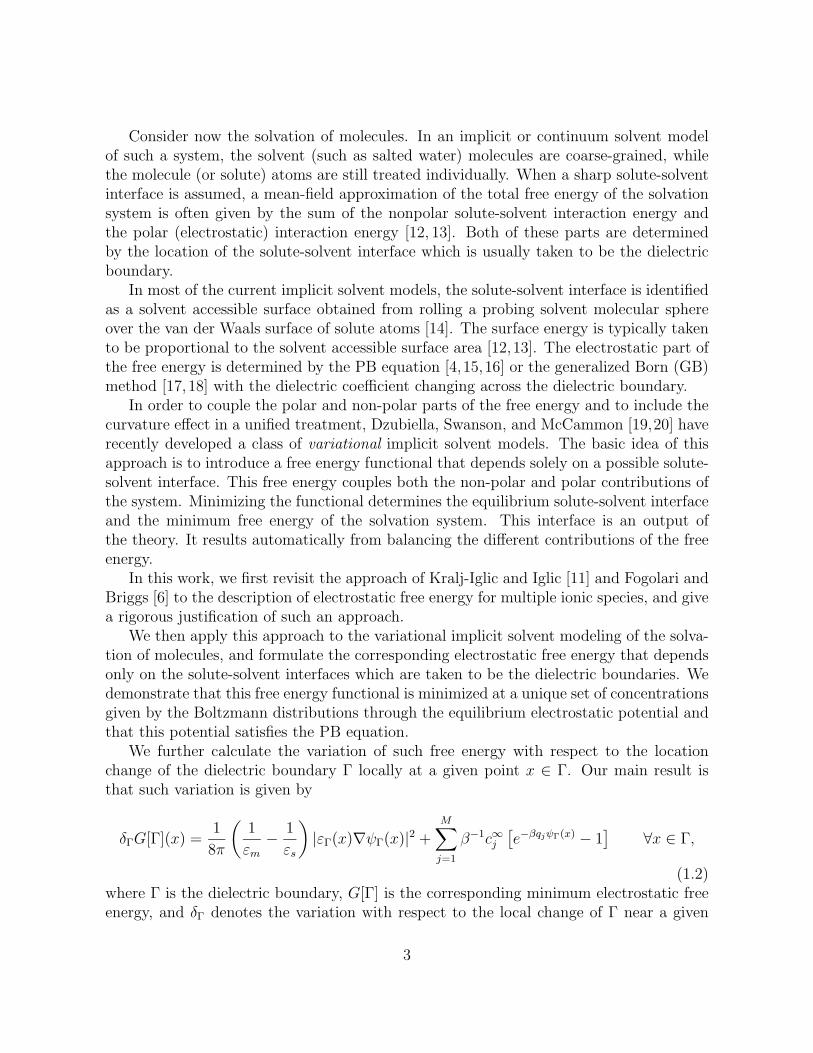
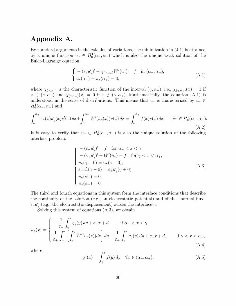
We now consider the solvation of molecules in the framework of variational implicit solventapproach [19,20]. We denote by Ω the entire region of an underlying solvation system. Itnow consists of the region of biomolecules (or solutes) Ωm, the region of solvent Ωs, andthe solute-solvent interface (or molecular surface) Γ that separates the solute and solventregions, cf. Figure 1. As usual, we assume that the interface Γ is also the dielectricboundary. This means that the dielectric coefficient in the system is a piecewise constantfunction:
εΓ(x) =
εm if x ∈ Ωm,
εs if x ∈ Ωs,
where εm and εs are the dielectric constants of the solutes (usually taken as that in thevacuum) and the solvent, respectively. We assume there are N atoms in the solute and
8
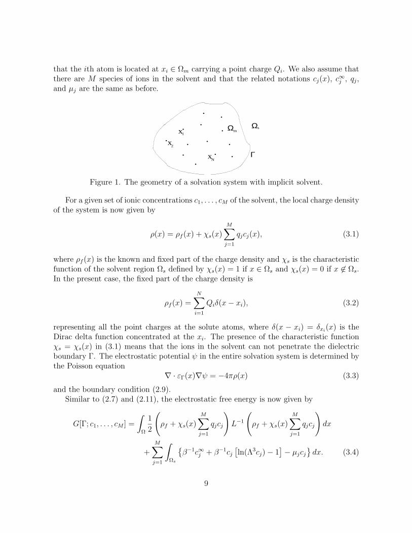
that the ith atom is located at xi ∈ Ωm carrying a point charge Qi. We also assume thatthere are M species of ions in the solvent and that the related notations cj(x), c∞j , qj,and µj are the same as before.
Γ
ΩΩx1
2
Nx
x
ms.
.
... .
.. .
.
..
.
Figure 1. The geometry of a solvation system with implicit solvent.
For a given set of ionic concentrations c1, . . . , cM of the solvent, the local charge densityof the system is now given by
ρ(x) = ρf (x) + χs(x)M
∑
j=1
qjcj(x), (3.1)
where ρf (x) is the known and fixed part of the charge density and χs is the characteristicfunction of the solvent region Ωs defined by χs(x) = 1 if x ∈ Ωs and χs(x) = 0 if x 6∈ Ωs.In the present case, the fixed part of the charge density is
ρf (x) =N
∑
i=1
Qiδ(x − xi), (3.2)
representing all the point charges at the solute atoms, where δ(x − xi) = δxi(x) is the
Dirac delta function concentrated at the xi. The presence of the characteristic functionχs = χs(x) in (3.1) means that the ions in the solvent can not penetrate the dielectricboundary Γ. The electrostatic potential ψ in the entire solvation system is determined bythe Poisson equation
∇ · εΓ(x)∇ψ = −4πρ(x) (3.3)
and the boundary condition (2.9).Similar to (2.7) and (2.11), the electrostatic free energy is now given by
G[Γ; c1, . . . , cM ] =
∫
Ω
1
2
(
ρf + χs(x)M
∑
j=1
qjcj
)
L−1
(
ρf + χs(x)M
∑
j=1
qjcj
)
dx
+M
∑
j=1
∫
Ωs
β−1c∞j + β−1cj
[
ln(Λ3cj) − 1]
− µjcj
dx. (3.4)
9
Notice that some of the integrals are taken over the solvent region Ωs, since the ionicconcentrations are zero in the solute region Ωm. Also, the osmotic pressure term isrelated to the volume of solvent region Ωs not the entire system region. Notice also thatthe free energy depends on Γ through the characteristic function χs(x) and the dielectriccoefficient εΓ(x) in the Poisson equation (3.3).
Repeating the calculations in the previous section and keeping in mind that all theconcentrations vanish in the solute region Ωm, we find that the free energy functional isminimized by a unique set of local ionic concentrations c1, . . . , cM in the solvent regionΩs. They are given by the Boltzmann distributions (cf. (2.2))
cj(x) = χs(x)c∞j e−βqjψ(x), (3.5)
where c∞j (1 ≤ j ≤ M) are given by (2.3). By (3.1)–(3.3) and (3.5), the equilibriumpotential ψ is the unique solution of the PB equation
∇ · εΓ(x)∇ψ + 4πχs(x)M
∑
j=1
qjc∞
j e−βqjψ = −4πρf (x) in Ω, (3.6)
together with the boundary condition (2.9). Similar to (2.12), the minimum free en-ergy, which is the free energy of the equilibrium system with equilibrium potential andconcentrations, is given by
G[Γ] = minc1,...,cM
G[Γ; c1, . . . , cM ]
=
∫
Ω
[
−εΓ(x)
8π|∇ψΓ|
2 + ρf (x)ψΓ − β−1χs(x)M
∑
j=1
c∞j(
e−βqjψΓ − 1)
]
dx, (3.7)
where ψΓ is the same as ψ that is the solution of the PB equation (3.6). We write ψΓ toemphasize its dependence on Γ.
Since the fixed charge density ρf consists of point charges centered at the soluteparticles xi (1 ≤ i ≤ N), the potential ψΓ determined by the PB equation (3.6) hassingularities at these points xi. Thus, the integral of |∇ψΓ|
2 is taken over the regionΩ minus a ball centered at xi with an infinitesimally small cut-off radii. We can alsoapproximate the delta functions in the fixed charge density by smooth functions of theGaussian distribution type so that the related integrals are regular. We will take thisview in some of our calculations below.
The issue of potential singularities can in fact be resolved rigorously. According toBorn’s definition [23], the electrostatic free energy is the reversible work needed to chargethe system. For a given set of local ionic concentrations c1, . . . , cM , the charge density isgiven by (3.1) and (3.2), and the corresponding potential is given by ψ = L−1ρ, where Lis defined by (2.8) (with ε(x) replaced by εΓ(x)) and the boundary condition (2.9). Thus,
10
the energy due to the point charges at solute atoms is
1
2
M∑
i=1
Qi (ψ − ψvac) (xi) =1
2
M∑
i=1
Qi
[
L−1
(
N∑
k=1
Qkδxk
)
− ψvac + L−1
(
χs
M∑
j=1
qjcj
)]
(xi),
where
ψvac(x) =N
∑
i=1
Qi
εm|x − xi|
is the reference potential generated by the point charges Qi at xi for all i = 1, . . . , N withthe dielectric constant εm. The energy due to the charge density
∑Mj=1 qjcj(x) is
1
2
M∑
j=1
∫
Ωs
qjcj(x)ψ(x)dx,
where the integral is over Ωs, since we assume the mobile ions can not penetrate the dielec-tric boundary. The other part of the free energy is contributed by the ionic concentrationsin the solvent that do not exist in the reference state. Thus, the total electrostatic freeenergy is
G[Γ; c1, . . . , cM ] =1
2
M∑
i=1
Qi
[
L−1
(
N∑
k=1
Qkδxk
)
− ψvac + L−1
(
χs
M∑
j=1
qjcj
)]
(xi)
+M
∑
j=1
∫
Ωs
1
2qjcjψ + β−1c∞j + β−1cj
[
ln(Λ3cj) − 1]
− µjcj
dx.
Notice that by Green’s formula
L−1(χscj)(xk) =
∫
Ωs
cj
(
L−1δxk
)
dx.
Thus, the variation of L−1(χscj)(xk) with respect to cj is L−1δxk. Repeating previous
calculations, we can thus obtain the Boltzmann distributions (3.5) for the equilibriumconcentrations and the PB equation (3.6) for the equilibrium potential now denoted byψΓ. These, together with the previous two equations for the free energy, lead to thecorresponding minimum electrostatic free energy that depends only on the solute-solventinterface Γ
G[Γ] =1
2
N∑
i=1
Qi (ψΓ − ψvac) (xi) −M
∑
j=1
∫
Ωs
[
1
2qjc
∞
j ψΓe−βqjψΓ + β−1c∞j(
e−βqjψΓ − 1)
]
dx.
(3.8)
11
Multiplying both sides of Eq. (3.6) by χsψ = χsψΓ, applying integration by parts, andusing the continuity of both ψΓ and εΓ∇ψΓ across Γ, we have
M∑
j=1
∫
Ωs
qjc∞
j ψΓe−βqjψΓdx = −
∫
Ωs
εs
4πψΓ∇
2ψΓdx
=
∫
Ωs
εs
4π|∇ψΓ|
2dx +
∫
Γ
1
4πψΓ
(
εΓ∂ψΓ
∂n
)
dS, (3.9)
where n denotes the unit normal at Γ pointing from Ωm to Ωs. This and (3.8) lead toanother form of the minimum free energy
G[Γ] =1
2
N∑
i=1
Qi (ψΓ − ψvac) (xi) −
∫
Ωs
εs
8π|∇ψΓ|
2dx −
∫
Γ
1
8πψΓ
(
εΓ∂ψΓ
∂n
)
dS
−M
∑
j=1
∫
Ωs
β−1c∞j(
e−βqjψΓ − 1)
dx. (3.10)
If we approximate the fixed point charges in (3.2) by a Gaussian type smooth functionthat vanishes on Ωs, still denoted by ρf , then the two formulas (3.7) and (3.10) only differby the ψvac part which is a constant with respect to the interface Γ. This follows fromthat the point charge part in (3.10) is just (1/2)
∫
ΩρfψΓdx minus the ψvac part and that
∫
Γ
1
4πψΓ
(
εΓ∂ψΓ
∂n
)
dS =
∫
Ωm
εm
4π|∇ψΓ|
2dx +
∫
Ωm
εm
4π
(
∇2ψΓ
)
ψΓdx
=
∫
Ωm
εm
4π|∇ψΓ|
2dx −
∫
Ω
ρfψΓdx.
3.2 Free energy variations with respect to the location change
of dielectric boundary
Fix an arbitrary point z ∈ Γ. We define the unit normal to Γ at z to be the one pointingfrom Ωm to Ωs. Consider a perturbation of the boundary near z. Let ∆V be the volumeof the difference between the perturbed and unperturbed boundaries. We assign such avolume a positive sign, if the perturbed boundary near z is on the positive side of thenormal direction of z with respect to the unperturbed boundary, and a negative signotherwise. Let ∆G[Γ, z] be the free energy of the perturbed boundary minus that of theunperturbed one. We define the variation of the free energy G[Γ] at z ∈ Γ with respectto the location change of Γ near z ∈ Γ in the normal direction to Γ to be the limitlim∆V →0 ∆G[Γ, z]/∆V , and denote it by δΓG[Γ](z) = δΓ,zG[Γ].
Given a function uΓ = uΓ(x) on Ω that depends on Γ. We define the variation of uΓ
with respect to the local change of boundary Γ near a point z ∈ Γ in the normal direction
12
at z to be a distribution and denote it by δΓ,zuΓ. For a perturbation of Γ locally near z,we denote by ∆uΓ,z the difference of uΓ and its perturbed one. Then, the variation δΓ,zuΓ
is defined by∫
Ω
δΓ,zuΓ(x)v(x)dx = lim∆V →0
1
∆V
∫
Ω
∆uΓ,z(x)v(x)dx
for any continuous function v on Ω.Fix z ∈ Γ. For convenience, we shall denote by δΓ the variation with respect to the
local change of Γ near z. Let ψΓ = ψ be the solution of the PB equation (3.6). By (3.7),we have
δΓG[Γ] =
∫
Ω
[
1
8πδΓ
(
1
εΓ(x)
)
|εΓ(x)∇ψ|2 −εΓ(x)
4π∇ψ · ∇δΓψ + ρf (x)δΓψ
]
dx
−
∫
Ω
(δΓχs(x))M
∑
j=1
β−1c∞j(
e−βqjψ − 1)
dx +
∫
Ω
χs(x)M
∑
j=1
qjc∞
j e−βqjψδΓψdx
=
∫
Ω
1
8πδΓ
(
1
εΓ(x)
)
|εΓ(x)∇ψ|2dx −
∫
Ω
(δΓχs(x))M
∑
j=1
β−1c∞j(
e−βq∞j ψ − 1)
dx,
(3.11)
where we used∫
Ω
[
−εΓ(x)
4π∇ψ · ∇δΓψ + χs(x)
M∑
j=1
qjc∞
j e−βqjψδΓψ
]
dx = −
∫
Ω
ρf (x)δΓψdx, (3.12)
which is obtained by multiplying both sides of the PB equation (3.6) by (1/4π)δΓψ andintegrating the resulting terms over Ω with the use of integration by parts.
Since ψ and εΓ∇ψ are continuous across the boundary Γ, we have by (3.11) andLemma 3.1 below that
δΓG[Γ](z) =1
8π
(
1
εm
−1
εs
)
|εΓ(z)∇ψ(z)|2 +M
∑
j=1
β−1c∞j(
e−βqjψ(z) − 1)
. (3.13)
A different argument is as follows. First, the given boundary Γ determines the potentialψ that is the solution of the PB equation (3.6). Now perturb Γ locally at a point z ∈ Γwith the perturbation of order τ . This leads to the variation of the dielectric coefficientεΓ + τδΓεΓ, up to the leading orders. This variation leads to the potential variationψ + τδΓψ, up to the leading orders. The corresponding free energy is then given by
G[ψ + τδΓψ] = G[ψ] + τδΓG + O(τ 2) as τ → 0.
On the other hand, it follows from (3.7) that
G[ψ + τδΓψ] =
∫
Ω
[
−1
8π(εΓ + τδΓεΓ)|∇(ψ + τδΓψ)|2 + ρf (ψ + δΓψ)
13
− (χs + δΓχs)M
∑
j=1
β−1c∞j(
e−βqj(ψ+τδΓψ) − 1)
]
dx + O(τ 2)
= G[ψ] + τ
∫
Ω
[
−1
4π∇ψ · δΓψ −
1
8πδΓεΓ|∇ψ|2 + ρfδΓψ
+ χs
M∑
j=1
qjc∞
j e−βqjψδΓψ + δΓχs
M∑
j=1
β−1c∞j(
e−βqjψ − 1)
]
dx + O(τ 2)
= G[ψ] + τ
∫
Ω
[
−1
8πδΓεΓ|∇ψ|2 + δΓχs
M∑
j=1
β−1c∞j(
e−βqjψ − 1)
]
dx + O(τ 2),
where we used (3.12). From the above two equations and Lemma 3.1 below, we obtainthe same result
δΓG[Γ](z) =
∫
Ω
[
−1
8πδΓεΓ|∇ψ|2 + δΓχs
M∑
j=1
β−1c∞j(
e−βqjψ − 1)
]
dx
=
∫
Ω
1
8πδΓ
(
1
εΓ
)
|εΓ∇ψ|2dx +
∫
Ω
δΓχs
M∑
j=1
β−1c∞j(
e−βqjψ − 1)
dx
=1
8π
(
1
εm
−1
εs
)
|εΓ(z)∇ψ(z)|2 +M
∑
j=1
β−1c∞j[
e−βqjψ(z) − 1]
. (3.14)
Let c∞ =∑M
j=1 c∞j > 0. Since the function f(t) = e−βψt − 1 for each ψ = ψ(z) isconvex, i.e., f ′′(t) > 0, we have by Jensen’s inequality that
M∑
j=1
c∞j[
e−βqjψ(z) − 1]
= c∞M
∑
j=1
c∞jc∞
[
e−βqjψ(z) − 1]
≥ c∞[
e−(βψ(z)/c∞)∑M
j=1 c∞j qj − 1]
= 0,
(3.15)where we used the electrostatic neutrality
∑Mj=1 qjc
∞j = 0. Therefore, since 0 < εm < εs,
the variation δΓG[Γ] of the electrostatic free energy with respect to the local locationchange of the dielectric boundary Γ, along the normal direction from Ωs to Ωs, is alwayspositive. Notice that −δΓG[Γ] is the normal component of surface force per unit surfacearea. Therefore, the resulting force is attractive to the solutes.
We end this section with the lemma used above.
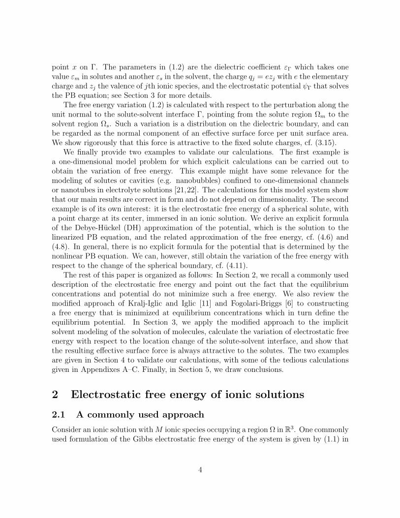
Lemma 3.1 Let uΓ = uΓ(x) be a piecewise constant function on Ω with
u(x) =
um if x ∈ Ωm,
us if x ∈ Ωs,
14
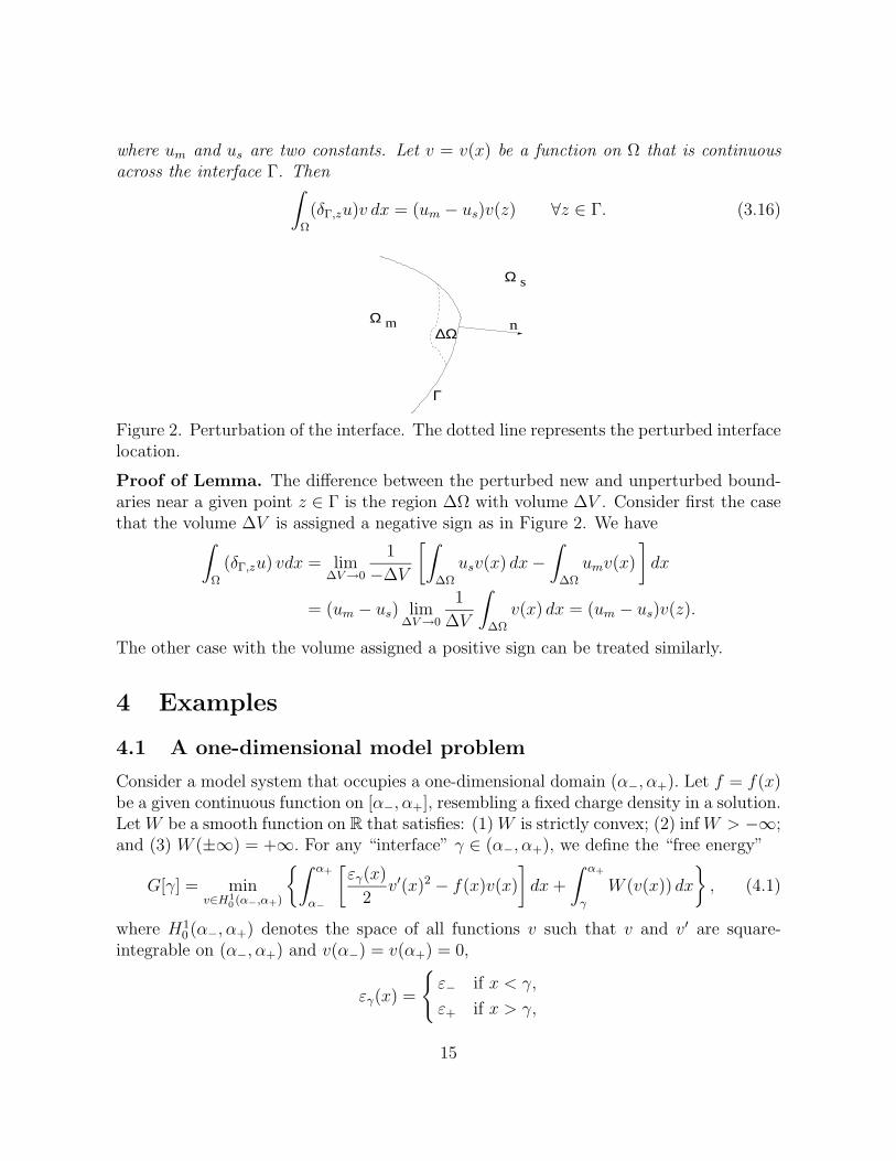
where um and us are two constants. Let v = v(x) be a function on Ω that is continuousacross the interface Γ. Then
∫
Ω
(δΓ,zu)v dx = (um − us)v(z) ∀z ∈ Γ. (3.16)
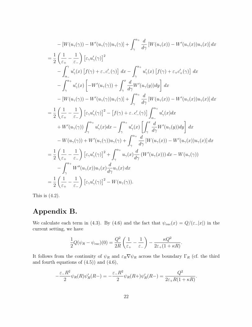
Γ
Ω
Ω
n∆Ω
m
s
Figure 2. Perturbation of the interface. The dotted line represents the perturbed interfacelocation.
Proof of Lemma. The difference between the perturbed new and unperturbed bound-aries near a given point z ∈ Γ is the region ∆Ω with volume ∆V . Consider first the casethat the volume ∆V is assigned a negative sign as in Figure 2. We have
∫
Ω
(δΓ,zu) vdx = lim∆V →0
1
−∆V
[∫
∆Ω
usv(x) dx −
∫
∆Ω
umv(x)
]
dx
= (um − us) lim∆V →0
1
∆V
∫
∆Ω
v(x) dx = (um − us)v(z).
The other case with the volume assigned a positive sign can be treated similarly.
4 Examples
4.1 A one-dimensional model problem
Consider a model system that occupies a one-dimensional domain (α−, α+). Let f = f(x)be a given continuous function on [α−, α+], resembling a fixed charge density in a solution.Let W be a smooth function on R that satisfies: (1) W is strictly convex; (2) inf W > −∞;and (3) W (±∞) = +∞. For any “interface” γ ∈ (α−, α+), we define the “free energy”
G[γ] = minv∈H1
0 (α−,α+)
∫ α+
α−
[
εγ(x)
2v′(x)2 − f(x)v(x)
]
dx +
∫ α+
γ
W (v(x)) dx
, (4.1)
where H10 (α−, α+) denotes the space of all functions v such that v and v′ are square-
integrable on (α−, α+) and v(α−) = v(α+) = 0,
εγ(x) =
ε− if x < γ,
ε+ if x > γ,
15

and ε− and ε+ are two positive constants, like the dielectric constants in the previoussections. Notice that the second integral in (4.1) is taken over (γ, α+). Up to a sign, thisterm resembles the Boltzmann distribution term in the PB free energy, cf. (3.7).
By a series of calculations that are summarized in Appendix A, we obtain the variationof the energy
G′[γ] =1
2
(
1
ε+
−1
ε−
)
[
εγu′
γ(γ)]2
− W (uγ(γ)) ∀γ ∈ (α−, α+). (4.2)
Notice that the functional G[γ] defined in (4.1) differs from G[Γ] in (3.7), among manyothers, by a sign. Thus, the result (4.2) agrees with our general formula (1.2) in the form.
4.2 A charged spherical solute in an ionic solution
Consider a spherical solute (colloid, macroion, protein, etc.) centered at the origin withradius R in an electrolyte solution. Assume the solute carries a single point charge Qat its center. Assume also there are M ionic species in the solvent with all the relatednotations cj(x), c∞j , ψ, qj, and µj same as before. The solute and solvent regions are
Ω−(R) = x ∈ R3 : |x| < R and Ω+(R) = x ∈ R
3 : |x| > R,
respectively, and the solute-solvent interface is
Γ = ΓR = x ∈ R3 : |x| = R.
We write εR = εΓ, ε− = εm, and ε+ = εs. Hence,
εR(x) =
ε− if |x| < R,
ε+ if |x| > R.
We also denote by χR the characteristic function of the solvent region Ω+(R). To indicatethe dependence on R, we denote the spherically symmetrical, equilibrium electrostaticpotential by ψR and write ψR(x) = ψR(r) for any x with |x| = r.
By (3.10), the free energy as a function of the radius R is given by
G[R] =1
2Q(ψR − ψvac)(0) −
ε+
2
∫
∞
R
|ψ′
R(r)|2r2dr −ε−R2
2ψR(R)ψ′
R(R−)
− 4πβ−1
M∑
j=1
c∞j
∫
∞
R
[
e−βqjψR(r) − 1]
r2dr. (4.3)
The derivative G′[R] will be derived below for the potential ψR determined by either thelinearized or the fully nonlinear PB equation.
16
If we perturb the spherical boundary of the solute by changing R to R + ∆R, thenthe volume change is
∆V =4π
3(R + ∆R)3 −
4π
3R3 = 4πR2∆R + O
(
(∆R)2)
.
Consequently, the variation of the free energy with respect to the location change of theboundary ΓR is
δRG[R] = lim∆V →0
G[R + ∆R] − G[R]
∆V=
G′[R]
4πR2. (4.4)
4.2.1 The Debye-Huckel approximation
The Debye-Huckel (DH) approximation of the electrostatic potential, still denoted by ψR,is the solution to the linearized PB equation
∇ · εR(x)∇ψR − ε+κ2χR(x)ψR = −4πQδ(x) in R3, (4.5)
together with some boundary condition which we assume to be ψR(∞) = 0. Here,
κ =
√
4πβ∑M
j=1 q2j c
∞j
ε+
defines the inverse electrostatic decay length (or ionic strength) of the solution. TheDB approximation is valid for weak electrostatic potentials and/or moderate to high saltconcentrations with high electrostatic screening.
The linearized PB equation (4.5) with our boundary conditions can be equivalentlywritten as
ε−∇2ψR = −4πQδ(x) for |x| < R,
∇2ψR − κ2ψ = 0 for |x| > R,
ψR(R − 0) = ψR(R + 0),
ε−ψ′
R(R − 0) = ε+ψ′
R(R + 0),
ψR(∞) = 0.
Solving this system of equations using the spherical symmetry, we get the DH potential
ψR(r) =
Q
R
(
1
ε+
−1
ε−
)
−κQ
ε+(1 + κR)+
Q
ε−rif r < R,
Q
ε+(1 + κR)re−κ(r−R) if r > R.
(4.6)
By (4.3) and a series of calculations that are presented in Appendix B, we obtain anapproximation of the free energy
G[R] =Q2
2R
(
1
ε+
−1
ε−
)
−κQ2(1 + 2κR)
4ε+(1 + κR)2
17
− 4πβ−1
M∑
j=1
c∞j
∫
∞
R
[
e−(pj/r)e−κ(r−R)
− 1]
r2dr, (4.7)
where pj = βqjQ/[ε+(1 + κR)]. If we further replace the exponential term by its linear
approximation and use the electrostatic neutrality∑M
j=1 qjc∞j = 0, we obtain
G[R] =Q2
2R
(
1
ε+
−1
ε−
)
−κQ2
2ε+(1 + κR). (4.8)
It then follows from (4.4) and (4.8) that the variation of the free energy G[R] with respectto the local change of the spherical boundary is
δRG[R] =Q2
8πR4
(
1
ε−−
1
ε+
)
+κ2Q2
2ε+(1 + κR)2,
which is always positive, since in general 0 < ε− < ε+.Notice that if there are no ions, then κ = 0 and thus the second term in G[R] in
(4.8) vanishes. The resulting formula is the classical Born’s formula. Notice also that anapproximation different from (4.8) will be obtained if we use the formula (3.8) insteadof (3.10), since the equivalence of these two formulas (3.8) and (3.10) follows from thenonlinear PB equation for the potential. However, different DH approximations onlydiffer by terms linear in the ionic strength κ. We shall pick up (4.8) and call it theBorn-Debye-Huckel (BDH) formula.
4.2.2 The fully nonlinear Poisson-Boltzmann description
Consider now the general case that the potential ψR is the solution to the fully nonlinearPB equation (cf. (3.6))
∇ · εΓ(x)∇ψR + 4πχR(x)M
∑
j=1
qjc∞
j e−βqjψR = −4πQδ(x) in R3, (4.9)
together with the boundary condition ψR(∞) = 0. In this case, we do not have anexplicit formula of the equilibrium potential ψR. But such potential exists and is unique.Moreover, the free energy is given by (4.3).
By a series of calculations presented in Appendix C, we obtain the derivative
G′[R] =Q2
2R2
(
1
ε−−
1
ε+
)
+ 4πR2β−1
M∑
j=1
c∞j[
e−βqjψR(R) − 1]
. (4.10)
It then follows from (4.4) that the variation of the free energy with respect to the locationchange of the boundary ΓR is
δRG[R] =Q2
8πR4
(
1
ε−−
1
ε+
)
+ β−1
M∑
j=1
c∞j[
e−βqjψR(R) − 1]
. (4.11)
18
Notice that G′[R] is the directional derivative along the direction of increasing the Rvalue, i.e., in the normal direction pointing from Ω− to Ω+. Notice also that by (C.3)|ε+ψ′
R(R+)| = |ε−ψ′R(R−)| = Q/R2. Therefore, if we apply our formula (1.2) (cf. also
(3.13)) with εm = ε−, εs = ε+, we get the same result.
5 Conclusions
In this work, we revisited the approach of Kralj-Iglic and Iglic [11] and Fogolari andBriggs [6] to the construction of electrostatic free energy of an ionic solution that dependsonly on the local ionic concentrations. We applied this approach to the variational implicitsolvent description of the solvation of molecules. The electrostatic free energy is nowdefined to be a functional of all possible solute-solvent interfaces that we take as dielectricboundaries.
Our key result is the formula (1.2) of the variation of such free energy with respectto the location change of the dielectric boundary. Such a variation defines the normalcomponent, along the normal pointing from the solute to solvent regions, of an effectivesurface force per unit surface area. Our analysis shows that this force is attractive tothe solute charges. This gives a quantitative interpretation in the frame work of implicitsolvent the following well known result: under the combined influence of electric fieldgenerated by solute charges and their polarization in the surrounding medium which iselectrostatic neutral, an additional potential energy emerges and drives the surroundingmolecules to the solutes; see [1].
The validation of our calculations is given through two examples. The first exampleis a one-dimensional model system which might have some relevance for the solvationin highly confined systems. In the second example which is of particular interest, weextended Born’s calculation of the free energy of a spherical solute with a point charge atits center to that for such a charged solute in an ionic solution. Within the DH (linearizedPB) approximation, the free energy and its variation are given by the classical Born’s freeenergy and its corresponding variation with corrections that are linear and quadratic,respectively, in the ionic strength in the limit of dilute ionic solution.
In our calculations, we used the zero Dirichlet boundary condition for the electrostaticpotential. The general case of non-zero Dirichlet boundary condition is of interest, sincethe resulting Boltzmann distribution can be different. This is worth of further study.
It is well-known that the approach based on the PB equation neglects steric effectsand correlation caused by the coarse structure of the solvent and the short-range repulsionbetween the ions. Some mean field models have been proposed to include the ionic stericeffects [5, 11]. One of our current studies is to apply our method of analysis to thesemodels.
19
Appendix A.
By standard arguments in the calculus of variations, the minimization in (4.1) is attainedby a unique function uγ ∈ H1
0 (α−, α+) which is also the unique weak solution of theEuler-Lagrange equation
− (εγu′
γ)′ + χ(γ,α+)W
′(uγ) = f in (α−, α+),
uγ(α−) = uγ(α+) = 0,(A.1)
where χ(γ,α+) is the characteristic function of the interval (γ, α+), i.e., χ(γ,α+)(x) = 1 ifx ∈ (γ, α+) and χ(γ,α+)(x) = 0 if x 6∈ (γ, α+). Mathematically, the equation (A.1) isunderstood in the sense of distributions. This means that uγ is characterized by uγ ∈H1
0 (α−, α+) and
∫ α+
α−
εγ(x)u′
γ(x)v′(x) dx+
∫ α+
γ
W ′(uγ(x))v(x) dx =
∫ α+
α−
f(x)v(x) dx ∀v ∈ H10 (α−, α+).
(A.2)It is easy to verify that uγ ∈ H1
0 (α−, α+) is also the unique solution of the followinginterface problem:
− (ε−u′
γ)′ = f for α− < x < γ,
− (ε+u′
γ)′ + W ′(uγ) = f for γ < x < α+,
uγ(γ − 0) = uγ(γ + 0),
ε−u′
γ(γ − 0) = ε+u′
γ(γ + 0),
uγ(α−) = 0,
uγ(α+) = 0.
(A.3)
The third and fourth equations in this system form the interface conditions that describethe continuity of the solution (e.g., an electrostatic potential) and of the “normal flux”εγu
′γ (e.g., the electrostatic displacement) across the interface γ.Solving this system of equations (A.3), we obtain
uγ(x) =
−1
ε−
∫ x
γ
gγ(y) dy + c−x + d− if α− < x < γ,
1
ε+
∫ x
γ
[∫ y
γ
W ′(uγ(z))dz
]
dy −1
ε+
∫ x
γ
gγ(y) dy + c+x + d+ if γ < x < α+,
(A.4)where
gγ(x) =
∫ x
γ
f(y) dy ∀x ∈ (α−, α+), (A.5)
20

and all c± = c±(γ) and d± = d±(γ) are constants that depend on γ. By the interfaceconditions (the third and forth equations in (A.3)) and the boundary conditions (the fifthand sixth equations in (A.3)), we obtain through a series of calculations
c− = c−(γ) =ε+
∆
[
1
ε+
∫ α+
γ
[∫ y
γ
W ′(uγ(z))dz
]
dy −1
ε+
∫ α+
γ
gγ(x) dx +1
ε−
∫ α−
γ
gγ(x) dx
]
,
c+ = c+(γ) =ε−∆
[
1
ε+
∫ α+
γ
[∫ y
γ
W ′(uγ(z))dz
]
dy −1
ε+
∫ α+
γ
gγ(x) dx +1
ε−
∫ α−
γ
gγ(x) dx
]
,
d− = d−(γ) =1
ε−
∫ α−
γ
gγ(x) dx − α−c−(γ),
d+ = d+(γ) = −1
ε+
∫ α+
γ
[∫ y
γ
W ′(uγ(z))dz
]
dy +1
ε+
∫ α+
γ
gγ(x) dx − α+c+(γ),
where
∆ = ∆(γ) = det
γ −γ 1 −1ε− −ε+ 0 0α− 0 1 00 α+ 0 1
= ε−(γ − α+) + ε+(α− − γ) < 0.
Setting v = uγ in (A.2), we get∫ α+
α−
f(x)uγ(x) dx =
∫ α+
α−
εγ(x)u′
γ(x)2dx +
∫ α+
γ
W ′(uγ(x))uγ(x)dx.
Thus, the free energy is given by (cf. (4.1))
G[γ] =
∫ α+
α−
[
εγ(x)
2u′
γ(x)2 − f(x)uγ(x)
]
dx +
∫ α+
γ
W (uγ(x))dx
= −1
2
∫ α+
α−
εγ(x)u′
γ(x)2dx +
∫ α+
γ
[W (uγ(x)) − W ′(uγ(x))uγ(x)] dx
= −ε−2
∫ γ
α−
u′
γ(x)2dx −ε+
2
∫ α+
γ
u′
γ(x)2dx +
∫ α+
γ
[W (uγ(x)) − W ′(uγ(x))uγ(x)] dx.
From (A.4) and (A.5), we can calculate u′γ(x) and (d/dγ)u′
γ(x). By (A.4) and thecontinuity of εγu
′γ at γ (cf. the fourth equation of (A.3)), we have ε−c−(γ) = ε+c+(γ),
and hence ε−c′−(γ) = ε+c′+(γ). Combining all these and the boundary conditions (cf. thelast two equations in (A.3)), we obtain the variation of the free energy at γ
G′[γ] = −1
2ε−
[
ε−u′
γ(γ − 0)]2
− ε−
∫ γ
α−
u′
γ(x)d
dγu′
γ(x) dx
+1
2ε+
[
ε+u′
γ(γ + 0)]2
− ε+
∫ α+
γ
u′
γ(x)d
dγu′
γ(x) dx
21
− [W (uγ(γ)) − W ′(uγ(γ))uγ(γ)] +
∫ α+
γ
d
dγ[W (uγ(x)) − W ′(uγ(x))uγ(x)] dx
=1
2
(
1
ε+
−1
ε−
)
[
εγu′
γ(γ)]2
−
∫ γ
α−
u′
γ(x)[
f(γ) + ε−c′−(γ)]
dx −
∫ α+
γ
u′
γ(x)[
f(γ) + ε+c′+(γ)]
dx
−
∫ α+
γ
u′
γ(x)
[
−W ′(uγ(γ)) +
∫ x
γ
d
dγW ′(uγ(y))dy
]
dx
− [W (uγ(γ)) − W ′(uγ(γ))uγ(γ)] +
∫ α+
γ
d
dγ[W (uγ(x)) − W ′(uγ(x))uγ(x)] dx
=1
2
(
1
ε+
−1
ε−
)
[
εγu′
γ(γ)]2
−[
f(γ) + ε−c′−(γ)]
∫ α+
α−
u′
γ(x)dx
+ W ′(uγ(γ))
∫ α+
γ
u′
γ(x)dx −
∫ α+
γ
u′
γ(x)
[∫ x
γ
d
dγW ′(uγ(y))dy
]
dx
− W (uγ(γ)) + W ′(uγ(γ))uγ(γ) +
∫ α+
γ
d
dγ[W (uγ(x)) − W ′(uγ(x))uγ(x)] dx
=1
2
(
1
ε+
−1
ε−
)
[
εγu′
γ(γ)]2
+
∫ α+
γ
uγ(x)d
dγ(W ′(uγ(x))) dx − W (uγ(γ))
−
∫ α+
γ
W ′′(uγ(x))uγ(x)d
dγuγ(x) dx
=1
2
(
1
ε+
−1
ε−
)
[
εγu′
γ(γ)]2
− W (uγ(γ)).
This is (4.2).
Appendix B.
We calculate each term in (4.3). By (4.6) and the fact that ψvac(x) = Q/(ε−|x|) in thecurrent setting, we have
1
2Q(ψR − ψvac)(0) =
Q2
2R
(
1
ε+
−1
ε−
)
−κQ2
2ε+(1 + κR).
It follows from the continuity of ψR and εR∇ψR across the boundary ΓR (cf. the thirdand fourth equations of (4.5)) and (4.6),
−ε−R2
2ψR(R)ψ′
R(R−) = −ε−R2
2ψR(R+)ψ′
R(R−) =Q2
2ε+R(1 + κR).
22
By (4.6) and integration by parts, we have
−ε+
2
∫
∞
R
|ψ′
R(r)|2r2dr = −Q2
2ε+(1 + κR)2
∫
∞
R
[
d
dr
(
e−κ(r−R)
r
)]2
r2dr
= −Q2
2ε+(1 + κR)2
∫
∞
R
(1 + κr)2
r2e−2κ(r−R)dr
= −Q2
2ε+(1 + κR)2
κ2
∫
∞
R
e−2κ(r−R)dr −
∫
∞
R
d
dr
[
e−2κ(r−R)
r
]
dr
= −κQ2
4ε+(1 + κR)2−
Q2
2ε+R(1 + κR)2.
The combination of these three equations, (4.3), and (4.6) leads to (4.7).Taylor expanding the exponential term in the last integral of (4.7) up to ψ2
R and usingthe electrostatic neutrality
∑Mj=1 qjc
∞j = 0, we obtain by (4.6) and a simple calculation
the approximation
−2πβ
∞∑
j=1
q2j c
∞
j
∫
∞
R
[ψR(r)]2r2dr = −κQ2
4ε+(1 + κR)2.
Replacing the last integral in (4.7) by this term, we obtain the BDH formula (4.8).
Appendix C.
The PB equation (4.9) and the boundary condition ψR(∞) = 0 are equivalent to
ε−∇2ψR = −4πQδ(x) for |x| < R,
ε+∇2ψR − 4π
M∑
j=1
qjc∞
j e−βqjψR = 0 for |x| > R,
ψR(R − 0) = ψR(R + 0),
ε−ψ′
R(R − 0) = ε+ψ′
R(R + 0),
ψR(∞) = 0.
(C.1)
Since ψR is spherically symmetric, the second equation in (C.1) becomes
d
dr
(
r2dψR
dr
)
= −4π
ε+
r2
M∑
j=1
qjc∞
j e−βqjψR(r) =: WR(r). (C.2)
Solving (C.1), we obtain
ψR(r) =
Q
ε−r+ d−(R) for |x| < R,
−
∫
∞
r
VR(s)ds −c+(R)
rfor |x| > R,
(C.3)
23
where
c+(R) = −Q
ε+
+
∫
∞
R
WR(r)dr,
d−(R) =Q
R
(
1
ε+
−1
ε−
)
−
∫
∞
R
VR(r)dr −1
R
∫
∞
R
WR(r)dr
are two constants with respect to x ∈ R3 but are dependent on R, and
VR(r) = −1
r2
∫
∞
r
WR(s)ds, (C.4)
WR(r) = −4π
ε+
r2
M∑
j=1
qjc∞
j e−βqjψR(r). (C.5)
By (4.3), the continuity of ψR and εR∇ψR across the boundary ΓR (cf. the third andfourth equations of (C.1)), and (C.3), we obtain
G[R] = Qd−(R) +Q2
2ε−R−
ε+
2
∫
∞
R
|ψ′
R(r)|2r2dr − 4πβ−1
M∑
j=1
c∞j
∫
∞
R
[
e−βqjψR(r) − 1]
r2dr.
Consequently,
G′[R] = Qd′
−(R) −Q2
2ε−R2+
ε+
2|ψ′
R(R + 0)|2R2 −
∫
∞
R
ε+
2r2 d
dR
(
|ψ′
R(r)|2)
dr
+ 4πβ−1
M∑
j=1
c∞j[
e−βqjψR(R) − 1]
R2 + 4πM
∑
j=1
qjc∞
j
∫
∞
R
e−βqjψR(r)
(
d
dRψR(r)
)
r2dr.
It follows from (C.1) and (C.3) that
ε+
2|ψ′
R(R + 0)|2R2 =R2
2ε+
|ε+ψ′
R(R + 0)|2 =R2
2ε+
|ε−ψ′
R(R − 0)|2 =Q2
2ε+R2.
By integration by parts, (C.2), (C.5), (C.1), and (C.3),
−
∫
∞
R
ε+
2r2 d
dR
(
|ψ′
R(r)|2)
dr
= −
∫
∞
R
ε+r2ψ′
R(r)
(
d
dRψ′
R(r)
)
dr
= −
∫
∞
R
ε+r2ψ′
R(r)d
dr
(
d
dRψR(r)
)
dr
=
[
−ε+r2ψ′
R(r)
(
d
dRψR(r)
)]∣
∣
∣
∣
r=∞
r=R+
+
∫
∞
R
ε+d
dr
(
r2ψ′
R(r))
(
d
dRψR(r)
)
dr
24
= ε+R2ψ′
R(R+)
(
d
dRψR(r)
)∣
∣
∣
∣
r=R+
+
∫
∞
R
ε+WR(r)
(
d
dRψR(r)
)
dr
= −Q
(
d
dRψR(r)
)∣
∣
∣
∣
r=R+
− 4πM
∑
j=1
qjc∞
j
∫
∞
R
r2e−βqjψR(r)
(
d
dRψR(r)
)
dr.
Combining the above three equations, we have
G′[R] =Q2
2R2
(
1
ε+
−1
ε−
)
+ 4πR2β−1
M∑
j=1
c∞j[
e−βqjψR(R) − 1]
+ Qd′
−(R) − Q
(
d
dRψR(r)
)∣
∣
∣
∣
r=R+
. (C.6)
Notice thatd
dR(ψR(R+)) =
(
d
dRψR
)
(r)
∣
∣
∣
∣
r=R+
+ ψ′
R(R+).
This, together with the continuity of ψR and εRψ′R at r = R and (C.3), implies that
−Q
(
d
dRψR(r)
)∣
∣
∣
∣
r=R+
= −Q
[
d
dR(ψR(R+)) − ψ′
R(R+)
]
= −Qd
dR(ψR(R−)) +
Qε+ψ′R(R+)
ε+
= −Qd
dR
[
Q
ε−R+ d−(R)
]
+Qε−ψ′
R(R−)
ε+
=Q2
ε−R2− Qd′
−(R) −Q2
ε+R2.
The insertion of this into (C.6) leads to (4.10).
Acknowledgments. This work is partially supported by the Deutsche Forschungsge-meinschaft (DFG) within the Emmy-Noether Programme (J. D.), by the US NationalScience Foundation (NSF) through grant DMS-0451466 (B. L.), and by the US Depart-ment of Energy through grant DE-FG02-05ER25707 (B. L.). Work in the McCammongroup is supported in part by NSF, NIH, HHMI, CTBP, NBCR, and Accelrys.
References
[1] Chu, B. Molecular Forces, Based on the Lecture of Peter J. W. Debye; Interscience,John Wiley & Sons, 1967.
25
[2] Israelachvili, J. Intermolecular and Surface Forces; Acdemic Press, 2nd ed., 1991.
[3] Reiner, E. S.; Radke, C. J. J. Chem. Soc. Faraday Trans. 1990, 86, 3901–3912.
[4] Sharp, K. A.; Honig, B. J. Phys. Chem. 1990, 94, 7684–7692.
[5] Borukhov, I.; Andelman, D.; Orland, H. Phys. Rev. Lett. 1997, 79, 435–438.
[6] Fogolari, F.; Briggs, J. M. Chem. Phys. Lett. 1997, 281, 135–139.
[7] Fogolari, F.; Zuccato, P.; Esposito, G.; Viglino, P. Biophys. Journal 1999, 76, 1–16.
[8] Gilson, M. K.; Davis, M. E.; Luty, B. A.; McCammon, J. A. J. Phys. Chem 1993,97, 3591–3600.
[9] Chou, T. IPAM Lecture Notes 2002.
[10] Allen, R.; Hansen, J.-P.; Melchionna, S. Phys. Chem. Chem. Phys. 2001, 3, 4177–4186.
[11] Kralj-Iglic, V.; Iglic, A. J. Phys. II (France) 1996, 6, 477–491.
[12] Roux, B.; Simonson, T. Biophys. Chem. 1999, 78, 1–20.
[13] Feig, M.; III, C. L. B. Current Opinion in Structure Biology 2004, 14, 217–224.
[14] Richards, F. M. Annu. Rev. Biophys. Bioeng. 1977, 6, 151–176.
[15] Davis, M. E.; McCammon, J. A. Chem. Rev. 1990, 90, 509–521.
[16] Fixman, M. J. Chem. Phys. 1979, 70, 4995–5005.
[17] Still, W. C.; Tempczyk, A.; Hawley, R. C.; Hendrickson, T. J. Amer. Chem. Soc.1990, 112, 6127–6129.
[18] Bashford, D.; Case, D. A. Ann. Rev. Phys. Chem 2000, 51, 129–152.
[19] Dzubiella, J.; Swanson, J. M. J.; McCammon, J. A. Phys. Rev. Lett. 2006, 96,087802.
[20] Dzubiella, J.; Swanson, J. M. J.; McCammon, J. A. J. Chem. Phys. 2006, 124,084905.
[21] Dzubiella, J.; Allen, R. J.; Hansen, J. P. J. Chem. Phys. 2004, 120, 5001–5004.
[22] Smeets, R. M. M.; Keyser, U. F.; Wu, M. Y.; Dekker, N. H.; Dekker, C. Phys. Rev.Lett. 2006, 97, 088101.
[23] Born, M. Z. Phys. 1920, 1, 45–48.
26