Electronic Thermal Conductance ofGraphene via Electrical Noise

a dissertation presentedby

Jesse Dylan Crossnoto

The School of Engineering and Applied Sciences

in partial fulfillment of the requirementsfor the degree of

Doctor of Philosophyin the subject ofApplied Physics

Harvard UniversityCambridge, Massachusetts

May 2017

©2017 – Jesse Dylan Crossnoall rights reserved.

Dissertation Advisor: Professor Philip Kim Jesse Dylan Crossno

Electronic Thermal Conductance of Graphene via ElectricalNoise

Abstract

This dissertation presents the methods and experimental results of studies on electronic thermal

transport in mesoscopic conductors by means of radio frequency Johnson noise thermometry. In

particular, we present the application of these methods to study the electronic thermal conductivity

of monolayer graphene over a wide range of temperatures, charge densities, and magnetic fields.

A comprehensive theory of thermal noise in conductors is formulated in a language convenient

for high frequency measurements of mesoscopic samples. Auto- and cross-correlated Johnson noise

thermometry is demonstrated over the temperature range of 3 − 300K and in magnetic fields up

to 13 T , achieving a sensitivity of 5.5mK (110 ppm) in 1 s of integration time. Techniques for

overcoming the challenges of measuring devices with resistances that dynamically vary over multi-

ple orders of magnitude are presented. Impedance matching circuits, capable of withstanding the

harsh measurement environments of condensed matter experiments while remaining stable across

the extreme changes in temperature and magnetic field, are described. A systematic and robust cali-

bration procedure for converting noise power to electronic temperature is outlined which allows for

the inevitable drift of device resistance that often plagues mesoscopic experiments. With the ability

to measure electronic temperature, the thermal conductance between the electronic system and a

iii

Dissertation Advisor: Professor Philip Kim Jesse Dylan Crossno

thermal bath can be measured.

We quantitatively discuss the various cooling mechanisms of the quasi-relativistic electrons in

graphene and how they combine to create a complicated thermal network. Moreover, we present ex-

perimental techniques to disentangle these mechanisms allowing the study of each cooling pathway

independently. Using these methods, the electron-phonon coupling of clean graphene is quanti-

tatively compared to theoretical estimates and found to be an order of magnitude larger than that

predicted for graphene intrinsic acoustic-phonons and the disorder-assisted supercollision mecha-

nism. We find that at low temperature and high carrier density, the thermal conductivity of diffusive

monolayer graphene closely obeys the Wiedemann-Franz law.

Near the charge neutrality point, we present evidence that the electronic system in monolayer

graphene forms an electron-hole plasma with collective behavior described by hydrodynamics. This

charge-neutral plasma of quasi-relativistic fermions, known as a Dirac fluid, exhibits a substantial

enhancement of the thermal conductivity, due to decoupling of charge and heat currents. We report

an order of magnitude increase in the thermal conductivity and the breakdown of the Wiedemann-

Franz law in the thermally populated charge-neutral plasma in graphene. A novel hydrodynamic

framework in the presence of charge disorder — in the form of a spatially varying chemical potential

— is presented and compared quantitatively to our experimental results.

Lastly, measurements for the low temperature thermal conduction of graphene under a mag-

netic field are presented. We report data spanning from zero field, through the quantum oscillation

regime, and into the quantum Hall regime.

iv

Contents

PageAbstract . . . . . . . . . . . . . . . . . . . . . . . . . . . . . . . . . . . . . . . . . . iiiAcknowledgments . . . . . . . . . . . . . . . . . . . . . . . . . . . . . . . . . . . . . ixCitations to previous publications . . . . . . . . . . . . . . . . . . . . . . . . . . . . . xii

1 Overview 1

2 Johnson noise thermometry 52.1 Thermal noise in resistors . . . . . . . . . . . . . . . . . . . . . . . . . . . . . . . 62.2 Resistor networks: The Johnson noise temperature . . . . . . . . . . . . . . . . . . 82.3 Johnson noise in RF circuits . . . . . . . . . . . . . . . . . . . . . . . . . . . . . . 112.4 An autocorrelation RF noise thermometer . . . . . . . . . . . . . . . . . . . . . . 122.5 Uncertainty in noise measurements . . . . . . . . . . . . . . . . . . . . . . . . . . 172.6 Impedance matching . . . . . . . . . . . . . . . . . . . . . . . . . . . . . . . . . 19

2.6.1 LC tank circuits . . . . . . . . . . . . . . . . . . . . . . . . . . . . . . . . . 202.6.2 Multi-stage matching . . . . . . . . . . . . . . . . . . . . . . . . . . . . . . 25

2.7 System noise temperature . . . . . . . . . . . . . . . . . . . . . . . . . . . . . . . 292.8 Calibration . . . . . . . . . . . . . . . . . . . . . . . . . . . . . . . . . . . . . . 332.9 Cross-correlated noise thermometry . . . . . . . . . . . . . . . . . . . . . . . . . . 37

2.9.1 multi-terminal cross-correlation . . . . . . . . . . . . . . . . . . . . . . . . . 40

3 Electronic cooling mechanisms in graphene 413.1 Wiedemann-Franz . . . . . . . . . . . . . . . . . . . . . . . . . . . . . . . . . . . 42

3.1.1 Linearization . . . . . . . . . . . . . . . . . . . . . . . . . . . . . . . . . . 443.1.2 Hot-electron shot noise . . . . . . . . . . . . . . . . . . . . . . . . . . . . . 44

3.2 Electron-Phonon coupling . . . . . . . . . . . . . . . . . . . . . . . . . . . . . . 453.2.1 Linearization . . . . . . . . . . . . . . . . . . . . . . . . . . . . . . . . . . 463.2.2 Bloch-Grüneisen temperature . . . . . . . . . . . . . . . . . . . . . . . . . . 473.2.3 Acoustic phonons . . . . . . . . . . . . . . . . . . . . . . . . . . . . . . . . 483.2.4 Optical phonons . . . . . . . . . . . . . . . . . . . . . . . . . . . . . . . . 49

3.3 Photon cooling . . . . . . . . . . . . . . . . . . . . . . . . . . . . . . . . . . . . 503.4 Thermal Network . . . . . . . . . . . . . . . . . . . . . . . . . . . . . . . . . . . 50

4 Thermal conductance via electrical noise 534.1 Rectangular devices . . . . . . . . . . . . . . . . . . . . . . . . . . . . . . . . . . 55

4.1.1 Electronic conduction only . . . . . . . . . . . . . . . . . . . . . . . . . . . 56

v

4.1.2 Phonon cooling only . . . . . . . . . . . . . . . . . . . . . . . . . . . . . . 594.2 Wedge devices . . . . . . . . . . . . . . . . . . . . . . . . . . . . . . . . . . . . . 604.3 Universality of β . . . . . . . . . . . . . . . . . . . . . . . . . . . . . . . . . . . . 634.4 Experimental setup . . . . . . . . . . . . . . . . . . . . . . . . . . . . . . . . . . 67

5 Thermal conductance in high density graphene 705.1 Device characteristics . . . . . . . . . . . . . . . . . . . . . . . . . . . . . . . . . 725.2 Thermal conductance . . . . . . . . . . . . . . . . . . . . . . . . . . . . . . . . . 74

6 The Dirac fluid 776.1 Temperature regimes . . . . . . . . . . . . . . . . . . . . . . . . . . . . . . . . . 786.2 Observation of the Dirac fluid and the breakdown of the Wiedemann-Franz law in

graphene . . . . . . . . . . . . . . . . . . . . . . . . . . . . . . . . . . . . . . . . 816.3 Sample Fabrication . . . . . . . . . . . . . . . . . . . . . . . . . . . . . . . . . . 926.4 Optimizing samples for high frequency thermal conductivity measurements . . . . . 926.5 Device Characterization . . . . . . . . . . . . . . . . . . . . . . . . . . . . . . . . 946.6 Bipolar Diffusion . . . . . . . . . . . . . . . . . . . . . . . . . . . . . . . . . . . 95

7 Hydrodynamic framework 987.1 Transport in inhomogeneous quantum critical fluids and in the Dirac fluid in graphene 100

7.1.1 Summary of Results . . . . . . . . . . . . . . . . . . . . . . . . . . . . . . . 1037.1.2 Outline . . . . . . . . . . . . . . . . . . . . . . . . . . . . . . . . . . . . . 108

7.2 Transport Coefficients . . . . . . . . . . . . . . . . . . . . . . . . . . . . . . . . . 1097.3 Relativistic Hydrodynamics . . . . . . . . . . . . . . . . . . . . . . . . . . . . . . 110

7.3.1 Hydrodynamic Equations . . . . . . . . . . . . . . . . . . . . . . . . . . . . 1117.3.2 Hydrodynamic Theory of Transport . . . . . . . . . . . . . . . . . . . . . . 115

7.4 The Dirac Fluid in Graphene . . . . . . . . . . . . . . . . . . . . . . . . . . . . . 1197.5 Numerical Results . . . . . . . . . . . . . . . . . . . . . . . . . . . . . . . . . . . 124

7.5.1 Comparison to Experiment . . . . . . . . . . . . . . . . . . . . . . . . . . . 1277.6 Phonons in Graphene . . . . . . . . . . . . . . . . . . . . . . . . . . . . . . . . . 1317.7 Conclusions . . . . . . . . . . . . . . . . . . . . . . . . . . . . . . . . . . . . . . 135

8 Magneto-thermal transport 1378.1 Generalized transport coefficients . . . . . . . . . . . . . . . . . . . . . . . . . . . 1388.2 Classical Hall Effect . . . . . . . . . . . . . . . . . . . . . . . . . . . . . . . . . . 1408.3 Graphene characteristics . . . . . . . . . . . . . . . . . . . . . . . . . . . . . . . . 1438.4 Electrical noise in high fields . . . . . . . . . . . . . . . . . . . . . . . . . . . . . . 1458.5 Magneto-thermal conductance . . . . . . . . . . . . . . . . . . . . . . . . . . . . 1498.6 Cyclotron radius . . . . . . . . . . . . . . . . . . . . . . . . . . . . . . . . . . . . 154

Appendix A RF cryostats 158A.1 Janis . . . . . . . . . . . . . . . . . . . . . . . . . . . . . . . . . . . . . . . . . . 160

vi

A.2 Oxford . . . . . . . . . . . . . . . . . . . . . . . . . . . . . . . . . . . . . . . . 162A.3 Leiden . . . . . . . . . . . . . . . . . . . . . . . . . . . . . . . . . . . . . . . . . 165

Appendix B Hydrodynamic framework 176B.1 Thermodynamics . . . . . . . . . . . . . . . . . . . . . . . . . . . . . . . . . . . 176

B.1.1 Thermodynamics of Disordered Fluids . . . . . . . . . . . . . . . . . . . . . 178B.2 Rescaling Symmetries of dc Transport . . . . . . . . . . . . . . . . . . . . . . . . . 181B.3 Weak Disorder . . . . . . . . . . . . . . . . . . . . . . . . . . . . . . . . . . . . . 182B.4 Equations of State of the Dirac Fluid . . . . . . . . . . . . . . . . . . . . . . . . . 185B.5 Numerical Methods . . . . . . . . . . . . . . . . . . . . . . . . . . . . . . . . . . 186

B.5.1 Finite Size Effects . . . . . . . . . . . . . . . . . . . . . . . . . . . . . . . . 188B.5.2 Dimensional Analysis . . . . . . . . . . . . . . . . . . . . . . . . . . . . . . 190

References 210

vii

Dedicated to Samantha Lucia Cardillo

viii

Acknowledgments

The past six years at Harvard have been some of the best in my life. The people I’ve met have

become some of my best friends. The colleagues I’ve worked with, both inside and outside of the

lab, have pushed me to grow and continue to inspire me to think bigger than I do. This dissertation

has been influenced by so many people that sitting down to write this acknowledgement seems more

overwhelming than the dissertation itself. Perhaps I should start with the single most influential

person in my life, the person to whom this text is dedicated. Samantha Cardillo has both supported

and encouraged me throughout my time at Harvard and before. We were traveling together when

we first found out that I was accepted to grad school and she celebrated, even knowing it meant

6+ years of stress, long hours, and late nights apart. We moved from sunny California to Boston

together where she helped me through the hardest times. Above all others, this thesis would not

have been possible without her.

While my path to graduation was certainly a windy one, I could not have asked for a better ad-

visor and mentor than Philip Kim. Philip has an unbelievable ability to provide support and un-

derstanding while still applying enough guidance and direction to keep me moving. I don’t think

I’ve ever met someone who cared more deeply for the well-being of their students than Philip. Plus,

probably the best meal I’ve had in years was at one of his now famous BBQs and how many other

ix

people get to say they beat their advisor at candle pin bowling.

It would be an understatement to say that this dissertation would not have happened without

the help of KC Fong. KC has affected, in some way, nearly every experiment in this thesis. He

helped design, guide, and interpret the Johnson noise thermometry experiments which realized

the observation of the Dirac fluid and it is safe to say he has taught me everything I know about mi-

crowave experiments. More than this though, I consider KC to be one of my closest friends.

I want to thank all the members of the Kim lab for helping me along the way. Jonah, Ke, Gil-

Ho, Xiaomeng, Jing, and Frank, these experiments only worked thanks to you sacrificing your time

scratching, transferring, fabricating, and brainstorming. Artem, Kemen and Hugo, the effort you

guys spent on building and optimizing the RF circuits and cyrostats was invaluable. Austin and

Andy, I likely would have gone crazy over the years without you guys there to distract me. I hope

you all take it as a compliment that one major reason I had to write this thesis from home was be-

cause, “I have WAY too many friends in lab to write productively”

Over the years, I was lucky enough to collaborate with some amazing people. In particular, I’d

like to thank Andy Lucas and Subir Sachdev for taking the time to really explain hydrodynamics in

terms that an experimentalist could understand. Thank you to all the folks at the Raytheon BBN,

especially Tom, Blake, Colm, and Graham, for going out of their way to patiently teach me how an

experiment should be run and Marcus, Mohammed, and Zach for all the great discussions over the

years. Thank you to the Yacoby and Capasso labs who were always there to lend tools, cryogenics,

and, most importantly, their expertise. And of course, Hannah Belcher, Carolyn Moore, and Bill

Walker for doing more than any person should to help me navigate the Harvard bureaucracy.

x

I can not overstate the great undergraduate education I received from the University of California

at Santa Barbara and the Santa Barbara City College. In particular, I owe my deepest gratitude to

Mike Young and Jim Allen for showing me what physics was and convincing me to give my educa-

tion a second chance and to Deborah Fygenson all her guidance over the years. Everyone knows an

undergraduate researcher is only as good as their graduate mentor and I was lucky enough to have

two great ones. Greg Dyer and Kim Weirich are two of the most patient and helpful people I’ve

known and I’m happy to now call them both friends. As any physics student who has gone through

Santa Barbara City College can tell you, at the heart of that program is Don Ion who seemed to

teach more with a question than any book could with a paragraph.

I want to thank the amazing friends I’ve made over the past years who have made my time in

Boston great. Bryan Kaye and Daniel Wintz have become two of my best friends and there isn’t a

doubt in my mind I would not have made it through without them. It’s hard to imagine a better

group of people than Zach Gault, Will Fitzhugh, Bryan Hassell, Pete Greskoff, and Michael Brady.

Evan Walsh, Tony Zhou, Danny Kim, Tommi Hakala, Rui Zhang, and Xi Wang were always there

for me. And even though they were mostly on the other side of the country, I want to thank Steve

Crawford, Brian Hoffman, Lucy Rangel, Will Snyders, Tommy Foley, Amber Mccreary, Kyle Lutz,

Norah Olley, Kevin Dober, Stephanie Hall, Greg Tavangar, Daniel Murawka, and Alex Woolf for

reminding me to keep my eye on graduation.

Finally, I cannot say enough about the love and support of family. Without the continual efforts

of my parents, Mark and Sally Crossno, and brother, Jordan Crossno, none of this would have been

possible.

xi

Previous publications

The experiments on thermal conduction in high density graphene and some of the experimental

details for measuring Johnson noise presented in Chapters 2–5 were published in

“Development of high frequency and wide bandwidth Johnson noise thermometry”

J. Crossno, X.Liu, T. Ohki, P. Kim, and K.C. Fong. Applied Physics Letters, 106(2),

p.023121 (2015).

The Dirac fluid experimental results shown in chapter 6 were published in

“Observation of the Dirac fluid and the breakdown of the Wiedemann-Franz law in

graphene”. J. Crossno, J.K. Shi, K. Wang, X. Liu, A. Harzheim, A. Lucas, S. Sachdev,

P. Kim, T. Taniguchi, K. Watanabe, T.A. Ohki, and K.C. Fong. Science, 351(6277),

pp.1058-1061 (2016).

The hydrodynamic theory of the Dirac fluid discussed in chapter 7 was published in

“Transport in inhomogeneous quantum critical fluids and in the Dirac fluid in graphene”.

A. Lucas, J. Crossno, K.C. Fong, P. Kim, and S. Sachdev. Physical Review B, 93(7),

p.075426 (2016).

xii

Sometimes science is a lot more art than science. A lot of

people don’t get that.

1Overview

This dissertation describes measurements of thermal transport in two-dimensional

systems. While it focuses primarily on extracting the electronic thermal conductivity of graphene,

the techniques described here are quite general. Probing the thermal characteristics in these ma-

terials requires a new thermometry technique capable of dealing with the challenges unique to

1

low-dimensional systems. Van der Waals heterostructures, for example, often contain several thin

electrical layers separated by atomic distances; precise knowledge of their individual temperatures is

critical in characterizing these structures. A good thermometer should have fast measurement times,

high accuracy, no magnetic field dependence, and a wide operating temperature range. Nanoscale

thermometry imposes additional challenges: the measurement process should be non-perturbative

to avoid thermal agitation of minute heat capacities, it should measure electron temperature directly

as weak electron-phonon coupling can result in different steady state electronic and lattice temper-

atures, it should be local and selective to distinguish temperatures of densely packed elements or

layers, and it should not require additional complicated processing of the device.

While the above requirements rule out many commonly used thermometry techniques, John-

son noise thermometry (JNT) stands out as a natural solution. Fundamentally based upon the

Fluctuation-Dissipation theorem, JNT is a primary thermometry having a straight forward inter-

pretation, independent of the material details. Analogous to radiation thermometry, JNT measures

temperature by passively monitoring fluctuations of the conducting components within the device

without the need for current excitations.

Chapter 2 outlines the fundamentals of Johnson noise thermometry and with a focus on measure-

ments of noise in mesoscopic systems at high frequency. A general framework for quantifying the

noise emitted by a device with a nonuniform spatial temperature profile is developed. We demon-

strate techniques for impedance matching devices with resistances which vary dynamically over mul-

tiple orders of magnitude. Experiments quantifying the performance of auto- and cross- correlated

JNT of a macroscopic resistor are presented.

2

Chapter 3 describes the various cooling mechanisms of hot electrons in low-dimensional systems.

The theoretical treatment of diffusive cooling of electrons in metals, known as the Wiedemann-

Franz Law, is presented as well as its limits in the high and low heating regimes. We then quanti-

tatively discuss the coupling of hot electrons to phonons with an emphasis on graphene electron-

phonon coupling.

Chapter 4 uses the foundations developed in the previous chapter to outline a technique to ex-

tract the electronic thermal conductivity using JNT paired with Joule heating. The intimate connec-

tion between dissipation (Joule heating) and fluctuations (Johnson noise) results in a measurement

which is insensitive to the device geometry or the form of the conductivity tensor.

Chapter 5 presents data on the thermal conductivity of monolayer graphene doped away from

the charge neutrality point. As expected for a degenerate Fermi liquid with a well defined Fermi

surface, we find good agreement to the Wiedemann-Franz law at low temperature. At high tem-

peratures we find electronic cooling to be dominated by coupling to phonons and we extract the

amplitude and thermal exponent characterizing the power transfer.

Chapter 6 details our experimental findings for graphene in the non-degenerate regime. Similar

to the data in chapter 5, at low temperatures we find that graphene obeys the Wiedemann-Franz

law while at sufficiently high temperatures electron-phonon coupling dominates. However at in-

termediate temperatures, we find that inter-particle scattering results in a decoupling of charge and

heat currents at the neutrality point and the Wiedemann-Franz law is violated. We compare this

strongly-interacting electron-hole plasma of quasi-relativistic fermions (known as a Dirac fluid) to

hydrodynamic theories with weak disorder.

3

Chapter 7 presents a hydrodynamic description of the Dirac fluid with disorder treated as a spa-

tially varying chemical potential. Based on relativistic conservation laws, the hydrodynamic equa-

tions are presented for two-dimensional systems to first order. The Dirac fluid in graphene is briefly

reviewed and placed in the context of these equations. The experimental data of chapter 6 is then

compared to numerical results of this hydrodynamic model.

Chapter 8 contains our most recent results on extending our thermal conduction measurements

of graphene into high magnetic fields. The generalized transport coefficients in two-dimensions

are defined in tensorial form and a description is given for their classical behavior in the presence

of a magnetic field. Thermal conductance of low temperature graphene is measured via Joule heat-

ing and Johnson noise from zero field to 13 T . We find quantum oscillations in the thermal signal

which diverge as the system enters quantum Hall.

Appendix A contains technical information about the measurement apparatus and Appendix B

contains details of the hydrodynamic calculations from chapter 7

4

In theory, theory and practice are the same thing, but in

practice...

Adam Savage

2Johnson noise thermometry

Given any process in which an applied force generates heat, the reverse process must

also exist and, therefore, thermal fluctuations must cause fluctuations in that force. The idea that

the same physics governing the dissipation of an object moving through some environment is re-

sponsible for the apparent random motion of that object was originally described by Einstein in

5

the context of pollen grains [1]. The generalized fluctuation-dissipation theorem [2] quantifies this

statement for linear systems† by relating the power spectral density SP (ω) to the real part of the

generalized impedanceZ(ω) [3].

SP (ω) ∝ kBT ℜ[Z(ω)] (2.1)

Nearly a quarter of a century later, Nyquist [4] related Einstein’s description of Brownian motion

to the electrical noise measured by Johnson [5, 6]. Although all the key components were in place, it

would take until 1946 for the first noise thermometer to be built [7]. The general idea is to measure

the noise spectrum emitted by a device and thus determine its electronic temperature. Johnson noise

thermometry (JNT) is analogous to radiation thermometry where the blackbody spectrum of an

object is used to determine its temperature — in fact, both rely upon modified versions of eq 2.1

2.1 Thermal noise in resistors

Johnson noise, often referred to as Johnson-Nyquist noise, was first measured in

1927 [5]. Johnson found the fluctuations in the squared voltage across a resistor were linearly pro-

portional to both the resistance and the temperature and independent of the conductor being mea-

sured. The following year, Nyquist derived the form of the noise spectral density through a simple

†Here a linear system is one where the force acting on a particle is proportional to its velocity — i.e. F/v isconstant

6

Figure 2.1: Schematic of Nyquist’s famous thought experiment. Two resistors in thermal equilibrium are connected

end to end and allowed to transfer energy between them via thermal current fluctuations.

thermodynamic argument. Consider two identical resistors in thermal equilibrium at a temperature

T connected such that any noise emitted by one is absorbed by the other, as shown in Fig. 2.1. As the

resistors are in thermal equilibrium, we know the power being absorbed by a given resistor per unit

frequency must be equal to the thermal energy being emitted, kBT . If we represent the Johnson

noise of the first resistor as a series voltage source with squared fluctuations, V 2JN , the power dissi-

pated in the second resistor per unit frequency is given by I2R =(VJN2R

)2R as the total resistance

of the circuit is 2R. Setting this equal to kBT/∆f leads us to Nyquist’s famous result.

SV (ω) = 4RkBT (2.2)

This derivation holds regardless of the conductor, be it an electrolytic solution or graphene in a

quantum Hall state. However, there is a glaring problem with extending this formula to high fre-

quency; similar to the UV-catastrophe in black-body radiation, Nyquist’s formula extends to infinite

energies as it lacks a high frequency cutoff. This is fixed by quantum mechanics resulting in a rolloff

7

of the noise spectrum centered at ℏω = kBT .

SV (ω) = 4ℏω ℜ(Z)

[1

2+

1

exp(ℏω/kBT )− 1

](2.3)

This high frequency cutoff was seen experimentally by Schoelkopf, et al. [8] and is only of practical

import at high frequencies (> 1GHz) and low temperatures (< 1K).

2.2 Resistor networks: The Johnson noise temperature

As noise is a random process, finding the spectral density of multiple resistors connected to-

gether into a network is not a simple matter of adding the voltages and/or currents via Kirchoff’s

laws, but instead the mean squared voltages ⟨V 2⟩ and/or mean squared current ⟨I2⟩must be com-

bined. This is a property of Gaussian distributed noise: adding together two Gaussian distributions,

each with mean 0 and variance σ, with result in another Gaussian distribution with mean 0 and

variance 2σ†.

To find the noise emitted by two resistors in series with resistanceR1 andR2 and temperature T1

and T2, we add their mean squared voltages.

⟨V 2⟩ = 4kB(R1T1 +R2T2)∆f (2.4)

†This is why mean squared error is often a useful metric. If errors are unbiased and Gaussian distributedthen summing their variance is appropriate.

8

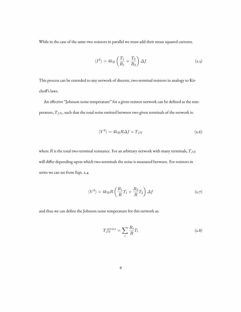
While in the case of the same two resistors in parallel we must add their mean squared currents.

⟨I2⟩ = 4kB

(T1

R1+

T2

R2

)∆f (2.5)

This process can be extended to any network of discrete, two-terminal resistors in analogy to Kir-

choff’s laws.

An effective “Johnson noise temperature” for a given resistor network can be defined as the tem-

perature, TJN , such that the total noise emitted between two given terminals of the network is:

⟨V 2⟩ = 4kBR∆f × TJN (2.6)

whereR is the total two-terminal resistance. For an arbitrary network with many terminals, TJN

will differ depending upon which two-terminals the noise is measured between. For resistors in

series we can see from Eqn. 2.4

⟨V 2⟩ = 4kBR

(R1

RT1 +

R2

RT2

)∆f (2.7)

and thus we can define the Johnson noise temperature for this network as:

T seriesJN =

∑i

Ri

RTi (2.8)

9

Similarly from Eqn.2.5 we see that for resistors in parallel

⟨V 2⟩ = ⟨I2⟩ ×R2 = 4kBR∆f(R

R1T1 +

R

R2T2) (2.9)

T parallelJN =

∑i

R

RiTi (2.10)

These equations are unified by considering the relationship between the power dissipated in a par-

ticular resistor Pi from a voltage across the two terminals of the network (or equally a current across

the network) compared to the total power dissipated over the entire network P0. For the resistors in

series Pi/P0 = Ri/R and for resistors in parallel Pi/P0 = R/Ri. Thus in both cases:

TJN =∑i

Pi

P0Ti (2.11)

In fact, this is quite general and holds for any combination of resistive elements. It stems from the

fluctuation dissipation theorem and can be summarized by the statement: The voltage fluctuations

created between two terminals of a resistor network due to the thermal fluctuations of a given ele-

ment in that network are exactly given by the normalized power dissipated in that element due to an

external voltage placed on those terminals.

In the continuous limit, Eqn. 2.11 can be used to find the noise emitted by a device with a spatially

non-uniform temperature profile T (r) by solving for the spatial power dissipation profileP(r).

TJN =

∫P(r) ∗ T (r)dr∫

P(r)dr(2.12)

10

where r is over the spatial dimensions of the device. Eqn. 2.12 is the main result of this section.

2.3 Johnson noise in RF circuits

When measuring Johnson noise at high frequency, it can be useful to reformulate the

problem into the language of microwave circuits. The Nyquist theorem, Eqn. 2.2, can be rewritten

to describe the average power, ⟨P⟩, absorbed by an amplifier coupled to a device with reflection

coefficient Γ 2:

⟨P⟩ = kBT∆f (1− Γ 2) (2.13)

and

Γ =Z − Z0

Z + Z0(2.14)

whereZ is the complex impedance of the device andZ0 is the characteristic impedance of the mea-

surement circuit — typically 50Ω. In this form is it quite easy to see the thermodynamic origins of

the Nyquist equation. A device at temperature T radiates a power of kBT per unit frequency; some

of that power is absorbed by the measurement circuit, and some is reflected back to the sample. All

the resistance dependence of the noise power is captured by Γ †. With this new formulation, the im-

portance of minimizing Γ becomes apparent. For high frequency Johnson noise thermometry to be

†this is also a nice proof for why Γ in any non absorptive 2 port device must be symmetric, Γ12 = Γ21. Ifthis was not true, we could place the device between two resistors in thermal equilibrium and one would heatthe other. Two-port devices which report asymmetric coefficients often include internally terminated thirdports.

11

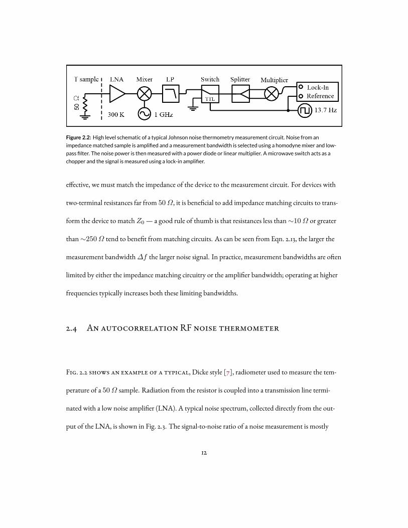
Figure 2.2: High level schematic of a typical Johnson noise thermometrymeasurement circuit. Noise from an

impedancematched sample is amplified and ameasurement bandwidth is selected using a homodynemixer and low-

pass filter. The noise power is thenmeasuredwith a power diode or linear multiplier. Amicrowave switch acts as a

chopper and the signal is measured using a lock-in amplifier.

effective, we must match the impedance of the device to the measurement circuit. For devices with

two-terminal resistances far from 50Ω, it is beneficial to add impedance matching circuits to trans-

form the device to matchZ0 — a good rule of thumb is that resistances less than∼10Ω or greater

than∼250Ω tend to benefit from matching circuits. As can be seen from Eqn. 2.13, the larger the

measurement bandwidth∆f the larger noise signal. In practice, measurement bandwidths are often

limited by either the impedance matching circuitry or the amplifier bandwidth; operating at higher

frequencies typically increases both these limiting bandwidths.

2.4 An autocorrelation RF noise thermometer

Fig. 2.2 shows an example of a typical, Dicke style [7], radiometer used to measure the tem-

perature of a 50Ω sample. Radiation from the resistor is coupled into a transmission line termi-

nated with a low noise amplifier (LNA). A typical noise spectrum, collected directly from the out-

put of the LNA, is shown in Fig. 2.3. The signal-to-noise ratio of a noise measurement is mostly

12

Figure 2.3: A typical spectrum collected directly from the output of a low noise amplifier (Miteq AU-1291,∼65 dBgain,∼100K noise temperature) with the input terminated with a 50Ω resistor. The spectrum is flat until the am-

plifier gain begins to roll off above 500MHz. The amplitude of the “white” spectrum is proportional to the resistor

temperature added to the amplifier noise temperature.

determined by the front-end LNA [9] so care should be taken in selecting the right amplifier. The

SiGe LNA (Caltech CITLF3) used throughout the majority of this thesis has a room temperature

noise figure, in the frequency range of 0.01 to 2GHz, of about 0.64 dB, corresponding to an in-

trinsic noise temperature of 46K .

Even though Johnson noise has a flat “white” spectrum, it is important to filter out unwanted

1/f low frequency fluctuations (≲ 100 kHz) as well as high frequency noise produced where

the amplifier gain begins to roll off. This can be done using high- and low- pass filters (producing a

spectrum similar to that shown in Fig. 2.4, or with a homodyne mixer and low-pass filter combo, as

shown in Fig. 2.2.

Once amplified and cleaned, the total noise power can be measured in a few ways: a spectrum

13

Figure 2.4: A typical Johnson noise spectrum after amplification and filtering using SMA high- and low-pass filters

(mini-circuits SLP and SHP series). This square band can then be integrated to find the total noise power and thus the

temperature of the resistor.

analyzer or digital Fourier transform can read the spectrum directly, a linear multiplier can square

the signal and the mean voltage can be measured, or a high frequency power diode and low pass

filter combo can convert the power to a proportional DC voltage. Each technique has its own advan-

tages/disadvantages and in a typical experiment multiple techniques are used.

When presented with a new device or noise setup, a spectrum analyzer is often the first measure-

ment to be done; it provides the most in-depth look into the noise of the system and readily shows

problem areas such as narrowband noise, parasitic resonances, and/or amplifier performance. Af-

ter initial setup, however, spectral detail becomes less important and measurements speeds can be

significantly enhanced by moving to an all analog setup.

A linear multiplier (as shown in the schematic Fig. 2.2) can be combined with an RF power split-

14

ter and a DC voltmeter to directly measure ⟨V 2⟩. Operating from DC to 2GHz, the multiplier†

serves as a square law detector with 30 dB dynamic range. A JNT using a multiplier is fast and has

the added capability of measuring the autocorrelation function, ⟨V (t)V (t − τ)⟩, by simply adding

a delay, τ , to one arm of the splitter. While more complicated to set up, once operational a multi-

plier is a good combination of speed and versatility.

The simplest of the three power detectors discussed here is an RF power diode/low-pass filter

combo (e.g. Pasternach PE8000-50). These detectors input an RF signal and output a DC voltage as

shown in Fig. 2.5. The output capacitance of these detectors can be quite large so, if a thermal mod-

ulation faster than a few 100Hz is required, care must be taken in choosing an appropriate model.

Nevertheless, this is the detector used most commonly in the experiments detailed in chapters 6 and

8 due to its wide dynamic range (30 dB), small sample package, and ease of use.

Once the noise power is converted to a DC voltage it can be read by a common voltmeter. To in-

crease the sensitivity it is useful to modulate the noise power. When measuring mesoscopic samples

this can be done by modulating the electron temperature via Joule heating. However, in the case of

a macroscopic resistor, a microwave switch can be placed after amplification to act as a chopper. The

resulting signal can then be integrated using a lock-in amplifier.

We can test the noise circuit shown in Fig. 2.2 by attaching a resistor to a coldfinger and varying

the temperature from 3K to 300K . The results are shown in Fig. 2.6. As the sample temperature

is lowered, the noise reduces linearly as expected from Eqn. 2.13. However, if we extrapolate the data

to zero temperature, we see residual noise; this offset is due to all the other (temperature indepen-

†Analog DevicesADL5931

15

Figure 2.5: Calibration curves for the Pasternach PE8000-50 power detector. Amonochromatic signal of known

power is supplied using amicrowave source (Stanford Research Systems) and the output is measured using a voltmeter

(Keithley 2400). The detector has a flat frequency response up to 1 GHz and shows linear behavior from -45 dBm to

-15 dBm (30 dB dynamic range)

16

Figure 2.6: Johnson noise of a 50Ω resistor measured by the circuit shown in Fig. 2.2. Inset show the lock-in amplifier

output. The signal is converted to noise power by the Nyquist equation. The solid line is a linear fit with an offset of

68 K due to amplifier noise

dent) noise sources in the system — primarily the front-end amplifier. It is useful to quantify this

offset in units of Kelvin and is often called the “system noise temperature”. Here we find a system

noise temperature of 68K using a room temperature amplifier. More details on this circuit can be

found in Ref. [10]

2.5 Uncertainty in noise measurements

Even noise has noise. There are 2main areas of uncertainty in a noise measurement. The first

comes from the fact that noise is stochastic and deals with how well you know the variance of a

Gaussian after measuring some amount of time. If the measurements you take are discrete and

17

Figure 2.7: 500 repeated Johnson noisemeasurements of a 50Ω resistor at 50K using two different measurement

bandwidths. The high bandwidth data has smaller statistical fluctuations than the low bandwidth data.

uncorrelated then we get the usual 1/√n dependence, but what do we do if we are measuring a

continuous signal? It turns out that this is an old problem which stems back to the 1940’s and mea-

surements of noise on telephone lines [11]. In 1944 Rice showed the effective number of uncorre-

lated measurements is related to the number of unique zero crossings of the signal and is given by

the product of the measurement time τ and the effective noise bandwidth† ∆f . The surprising fact

that the wider the measurement bandwidth the lower the uncertainty, is counter to many experi-

ments where high Q filters are desired to lower the background noise; nevertheless, it can be seen

experimentally, as shown in Fig. 2.7

The second source of uncertainty comes from external noise sources, such as amplifiers, and boils

down to the question: of the noise you measure, what amount comes from the sample? Quantita-

tively, this can be thought of as a constant offset to the sample temperature and is called the system

noise temperature Tn‡. In an autocorrelated noise measurement, Tn can be estimated as the offset of

†The effective noise bandwidth is defined as the width of a perfect square band that passes the same noisepower as the true filter function.

‡It should be noted that the system noise temperature can be quite different from an amplifiers intrinsic

18

a linear fit to the noise power vs sample temperature, as shown in Fig. 2.6. This offset is highly sen-

sitive to the noise in the front-end amplifier, the sample impedance matching, and the bandwidth

being measured, as discussed in section 2.7.

Combining these two sources of error we arrive at the famous Dicke radiometer formula [7]:

δT =T + Tn√τ ∆f

(2.15)

where δT is the uncertainty in the measured temperature.

We can directly compare Eqn. 2.15 to experiments by repeating a measurement many times and

studying how it fluctuates about the mean. Fig. 2.8 compares two histograms, both containing

20, 000 autocorrelation measurements at 50K with 50ms integration time but using two differ-

ent bandwidths: 28 and 328MHz. A sensitivity of 5.5mK (110ppm) in 1 second of integration

time was achieved using 328MHz bandwidth on a 50K signal.

2.6 Impedance matching

Life does not always give you 50Ω samples. Eqn. 2.13 illustrates the importance of min-

imizing the impedance mismatch between the sample and the measurement circuitry – typically

50Ω. The central principle is to use non-dissipative components to transform the total impedance

noise temperature which often assumes a perfectly matched input impedance. See the section 2.7 for moredetails

19

Figure 2.8: Histograms of 20,000 auto-correlation temperaturemeasurements for 28 and 328MHz bandwidth

using 50ms integration time. Histogram peaks are normalized to 1 for clarity. All data is taken on a 50K resistive

load.

Figure 2.9: Schematic of an LC tank circuit setup in a low-pass configuration used to transform a sample resistanceR0

to match the characteristic impedance of ameasurement circuitZ0.

toZ(ω0) = 50+0i Ω at some frequency ω0. Impedance matching mesoscopic devices has a unique

set of challenges: electrostatic gates and high magnetic fields can cause device impedances to change

by multiple orders of magnitude, cryogenic temperatures require the use of only thermally stable

components, and large magnetic fields restrict the use of ferrite inductors.

2.6.1 LC tank circuits

A common way to achieve matching is to use an LC circuit. These transformation circuits,

known as a tank circuits, can be arranged in several ways but the configuration most useful to these

20

experiments is that of a low-pass filter — i.e a shunt capacitor followed by a series inductor as shown

in Fig. 2.9. The impedance of such a circuit is given by:

Z(ω) =(R −1

0 + iωC)−1

+ iωL (2.16)

whereL andC are the series inductance and shunt capacitance values, respectively. Proper matching

requires solving Eqn. 2.16 under the condition:

Z(ω0) = 50 + 0i Ω (2.17)

where ω0 is the center of the measurement band. Fig. 2.10 shows a plot of the real and imaginary

components of Eqn. 2.16 withR0 = 1 kΩ. For the right choice ofC andL, the imaginary part of

the complex impedance crosses zero when the real part is 50Ω. Combining Eqn. 2.16 and Eqn. 2.17

for a givenR0, ω0 andZ0 gives us the needed inductance and capacitance values.

L =

√R0Z0

ω 20

C =1√

R0Z0ω 20

(2.18)

While in theory adding a precise inductance and capacitance to a device is straight forward, in

practice real devices can have a not insignificant amount of stray capacitance†. To account for this we

can use a variable capacitor and tune the matching circuit to each device. One simple, temperature

†stray inductance is also possible (particularly if long wire bonds are necessary) but is usually negligible forthe resistance and frequency ranges in this thesis

21

Figure 2.10: The real and imaginary impedance of an LC tank circuit (Eqn. 2.16) withR0 = 1 kΩ,C = 4.5 pF , and

L = 220nH . The imaginary component cross zero as the real component is 50Ω.

independent, magnetic field compatible capacitor that can be easily tuned is a set of twisted pair

wires. Fig. 2.11 shows an example of a matching circuit using a twisted pair capacitor before and after

tuning.

A vector network analyzer (VNA) is used to measure the sample reflectance Γ 2 = S211 to ensure

the sample is properly matched. Fig. 2.12 shows how the reflectance changes for a 1 kΩ sample resis-

tance and 220 nH series inductance as the capacitance is tuned. When properly tuned we measure a

large dip in S211 signifying the sample is well coupled to the 50Ω transmission line.

After matching, the noise spectral density emitted into the measurement circuitry is no longer

flat but instead shaped by Γ in accordance to Eqn. 2.13. This point becomes clear when looking at

the noise spectra emitted by an impedance matched sample at various temperatures — as shown

in Fig. 2.13. Two features of these spectra stand out prominently: first, the background noise is no

longer flat but has structure and, second, the increase in noise as the sample temperature is raised

22

Figure 2.11: Images of an impedancematching circuit before (le ) and after (right) capacitance tuning. A long piece of

twisted pair wire shunts the sample and an inductor (Coilcraft RF Air Core) is placed in series. To tune the capacitance,

the twisted pair wire is cut shorter and shorter while the reflectance is monitored.

Figure 2.12: Reflectance curves while tuning amatching circuit forR0 = 1 kΩ andL = 200nH . The rightmost

curve (green) corresponds to the lowest capacitance and the leftmost curve (blue) corresponds to the highest. Each

curve is the result of cutting off a section of twisted pair wire as shown in Fig. 2.11.

23

Figure 2.13: Amplified noise spectrum from a device, impedancematched using an LC tank circuit, at various temper-

atures. The background noise is no longer flat as the amplifier is not properly terminated at all frequencies. As the

device temperature is raised, the spectral density increases non-uniformly as different frequencies couple differently

to the circuitry as determined by Eqn. 2.13

is not the same at all frequencies. The result is that we are no longer free to select just any measure-

ment bandwidth but must carefully choose filters suited to the reflection profile.

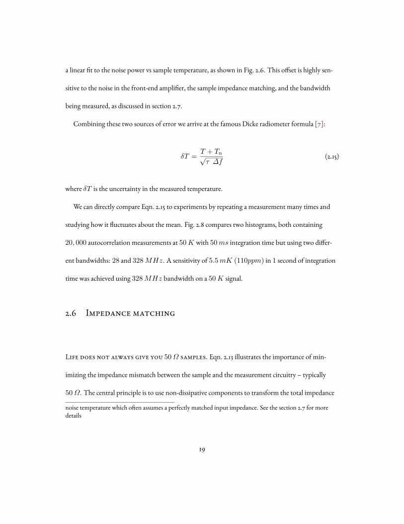
In most mesoscopic measurements, the resistance of the device under test varies throughout the

experiment; whether electrostatic gates modulate the carrier density, strong magnetic fields drive the

system into quantum hall, or cryogenic temperatures modify the conductivity, matching networks

should operate over a wide dynamic range of input impedances. The response of a single stage LC

matching network coupled to a variable resistance device† is shown in Fig. 2.14. The device is opti-

mally matched around 450Ω but maintains more than 10 dB coupling between 200Ω and 1 kΩ.

As the resistance drops, we see the appearance of the trivial solution to Eqn. 2.16 ofR0 = 50Ω and

†in this case a graphene device modulated via an electrostatic gate

24

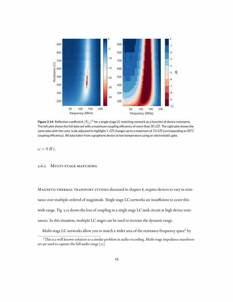
Figure 2.14: Reflection coefficient |S11|2 for a single stage LCmatching network as a function of device resistance.

The left plot shows the full data set with amaximum coupling efficiency of more than 30 dB. The right plot shows the

same data with the color scale adjusted to highlight 1 dB changes up to amaximum of 10 dB (corresponding to 90%coupling efficiency). All data taken from a graphene device at low temperature using an electrostatic gate.

ω = 0Hz.

2.6.2 Multi-stage matching

Magneto-thermal transport studies discussed in chapter 8, require devices to vary in resis-

tance over multiple ordered of magnitude. Single stage LC networks are insufficient to cover this

wide range. Fig. 2.15 shows the loss of coupling in a single stage LC tank circuit at high device resis-

tances. In this situation, multiple LC stages can be used to increase the dynamic range.

Multi-stage LC networks allow you to match a wider area of the resistance-frequency space† by

†This is a well known solution to a similar problem in audio recording. Multi-stage impedance transform-ers are used to capture the full audio range [12].

25

Figure 2.15: Reflectionmeasurements of a single stage LC tank circuit coupled to a graphene device at different resis-

tances. At high resistance the coupling drops off and reflection is high.

Figure 2.16: Schematic of a double-stage LCmatching network. The device resistanceR0 is transformed tomatch the

characteristic impedance of themeasurement circuitZ0 using two LC tank circuits. This results in a wider matching

bandwidth and/or larger dynamic range depending on the values of the reactive elements.

giving you multiple solutions to the equationZ(ω) = Z0. An example schematic of a two-stage LC

tank circuit is shown in Fig. 2.16. The resulting impedance takes the form:

Z(ω) =

[(R −1

0 + iωC1

)−1+ iωL1

] −1+ iωC2

−1

+ iωL2 (2.19)

Eqn. 2.19, under the constraint defined by Eqn. 2.17, can have multiple solutions for the same set

26

Figure 2.17: Real and imaginary components of Eqn. 2.19 forR = 1 kΩ,C1 = 1.9 pF ,L1 = 430nH ,C2 =8.6 pF , andL2 = 96nH . The impedance goes to 50 + 0iΩ at two nearby frequencies.

of inputs. This makes it possible to increase the matching bandwidth for the same dynamic range.

Fig. 2.17 plots the real and imaginary components of Eqn. 2.19 for a specific choice of inductances

and capacitances designed to cross 50+0i Ω at two nearby frequencies for the same device resistance.

It can be shown for a fixed resistance that the maximum bandwidth occurs when the impedance is

dropped by geometric factor [9] — i.e each stage transforms the impedance by the same multiplica-

tive factor. For anN stage network of the form shown in Fig. 2.16, the ith inductance and capaci-

tance are given by a generalized form of Eqn. 2.18.

Li =

(R 2N−2i+1

0 Z 2i−10

)1/2N

ω0Ci =

(R 2N−2i+1

0 Z 2i−10

)−1/2N

ω0(2.20)

Applying Eqn. 2.20 to a two-stage LC network with a graphene device we can increase the matched

bandwidth to∼150MHz, as shown in Fig. 2.18.

However, if instead we want to match to larger range of resistances, we can move one of the so-

27

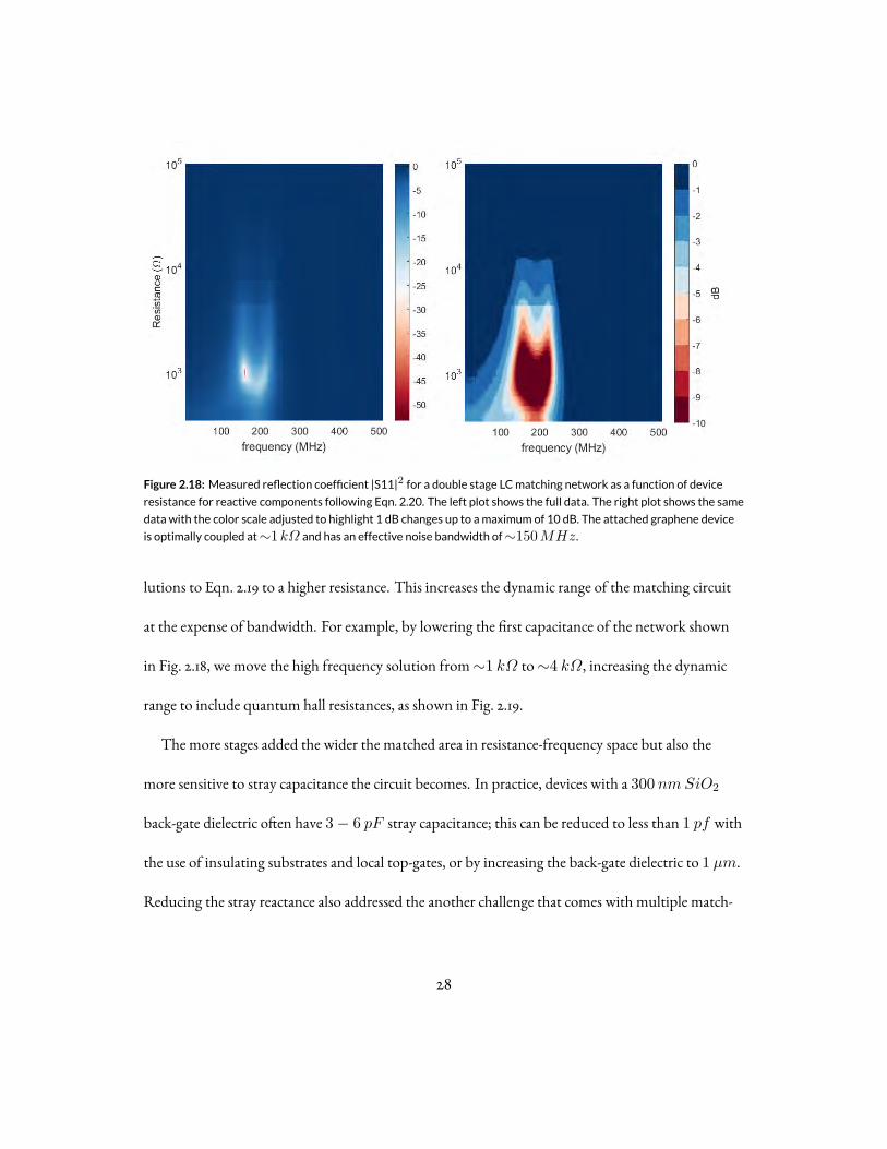
Figure 2.18: Measured reflection coefficient |S11|2 for a double stage LCmatching network as a function of device

resistance for reactive components following Eqn. 2.20. The left plot shows the full data. The right plot shows the same

data with the color scale adjusted to highlight 1 dB changes up to amaximum of 10 dB. The attached graphene device

is optimally coupled at∼1 kΩ and has an effective noise bandwidth of∼150MHz.

lutions to Eqn. 2.19 to a higher resistance. This increases the dynamic range of the matching circuit

at the expense of bandwidth. For example, by lowering the first capacitance of the network shown

in Fig. 2.18, we move the high frequency solution from∼1 kΩ to∼4 kΩ, increasing the dynamic

range to include quantum hall resistances, as shown in Fig. 2.19.

The more stages added the wider the matched area in resistance-frequency space but also the

more sensitive to stray capacitance the circuit becomes. In practice, devices with a 300 nmSiO2

back-gate dielectric often have 3− 6 pF stray capacitance; this can be reduced to less than 1 pf with

the use of insulating substrates and local top-gates, or by increasing the back-gate dielectric to 1 µm.

Reducing the stray reactance also addressed the another challenge that comes with multiple match-

28

Figure 2.19: Measured reflection coefficient |S11|2 for the same double stage LCmatching network shown in Fig. 2.18

as a function of device resistance with the first stage capacitance lowered. This moves the high frequency solution

to a higher resistance; effectively increasing the dynamic range at the cost of bandwidth. This technique enables the

continuousmeasurement of graphene devices from zero field into the quantumHall regime

ing stages — it is no longer trivial to tune the circuit using a gimmick†. For these more complicated

networks, surface mount ceramic capacitors can be soldered directly to the sample package, as shown

in Fig. 2.20, and adjustments can be made by careful removal and replacement‡.

2.7 System noise temperature

A factor of two in signal to noise can be the difference between graduating in two years

and eight. From the Dicke radiometer formula, Eqn. 2.15, the measurement time scales as the system

noise temperature squared. Each component of the measurement circuit should be chosen with this

†twisted pair wire is one form of a gimmick used to fine tune the circuit capacitance‡making sure to only apply heat the capacitor locally to avoid damaging the sample.

29

Figure 2.20: Image of a two-stage LCmatching network soldered directly to a custom cryogenic sample package and

wire-bonded to a graphene device. Inductive elements have gold leads allowing direct wire-bonding. The sample is

placed on an insulating sapphire substrate with a local top-gate to reduce the stray capacitance.

in mind and, as such, it is important to understand how each element affects the system as a whole.

The system noise temperature, Tn, is the temperature at which your sample emits the same noise

power as the sum of all the “unwanted” noise in your system — i.e. your signal to noise ratio is given

by T/Tn, where T is the sample temperature. Quantifying noise in this way lets us write the output

voltage of our circuit, Vout, (which is proportional to the integrated noise power) as:

Vout = G(Γ )(T + Tn(Γ )) (2.21)

where Γ 2 is reflection coefficient between the sample and the amplifier and G is a generalized gain

factor set by the LNA amplification together with the insertion loss of the microwave components

integrated over the bandwidth defined by the external filters. In general, both G and Tn are func-

tions of Γ . All defining characteristics of a given measurement circuit can be swept into Tn and G.

In principle these factors must be measured but reasonable estimates can aid in the circuit design.

30

It is useful to distinguish the difference between the intrinsic noise temperature Tn0 and the sys-

tem noise temperature Tn. Tn0 corresponds to the noise emitted by the circuit relative to the John-

son noise of a perfectly matched resistor, while Tn is relative to the sample being measured — i.e. Tn0

can be reported on a device’s specification sheet while Tn is a function of the sample under test and

can therefore change with experimental parameters such as electrostatic gate voltage and external

magnetic field. In general Tn is always equal to or greater than Tn0 .

While Tn0 is primary determined by the front-end amplifier, every component, i, with a finite

intrinsic noise Tni contributes an amount inversely proportional to the gain before that component,

Gi. For example, if a circuit has three amplification stages with gainsG1,G2, andG3 with intrinsic

noise temperatures Tn1 , Tn

2 , and Tn3 , respectively, the total system intrinsic noise value is given by:

Tn0 = Tn

1 +Tn2

G1+

Tn3

G1G2(2.22)

or in general

Tn0 =

∑i

Tni∏

j<iGj(2.23)

Hence, if the front-end amplifier has a gain or 30 dB, the noise from second amplifier is effectively

reduced by a factor of 1, 000.

Estimating Tn from Tn0 requires knowing the matching function characterized by Γ . If Γ is

frequency independent then Tn ≈ Tn0 /(1 − Γ 2). For arbitrary Γ (ω) you can integrate over the

31

Figure 2.21: Schematic of a common noisemodel for active elements. A random voltage source is added in series with

the signal and a random current source is added in parallel.

bandwidth defined by external filters∆f †.

Tn ≈ 1

∆f

∫∆f

T 0n

1− Γ 2(ω)dω (2.24)

The above formulation is approximate as it assumes the system’s intrinsic noise can be described

entirely by a single parameter Tn0 — a good assumption if the sample is properly matched. However,

in general active components require two parameters to fully capture the noise behavior. A com-

mon technique is to model the circuit with an effective series voltage noise and parallel current noise,

as shown in Fig. 2.21. However, an equivalent description, which is often more useful in microwave

experiments, is that of a forward traveling noise power, Tnfor, a reverse traveling noise power Tn

rev ,

and some correlation between them. In the case of perfect matching, Γ → 0, Tnrev is completely

absorbed. However for finite Γ we can write the amplified noise as:

⟨P ⟩ = G[T (1− Γ 2) + Tn

revΓ2 + Tn

for

](2.25)

†Eqn. 2.24 approximates the external filter function as a perfect square filter of bandwidth∆f . For thefull calculation you must include the full filter function.

32

Rewriting this in the form of Eqn. 2.21 and solving for Tn and G yields.

Tn(Γ ) =Γ 2

1− Γ 2Tnrev +

1

1− Γ 2Tnfor (2.26)

and

G(Γ ) = G(1− Γ 2) (2.27)

Eqn. 2.26 is what determines the measurement uncertainty and therefore the speed of the mea-

surement. An interesting consequence of Eqn. 2.25 is that when the sample temperature is equal to

Tnrev , the total output noise has no dependence on Γ ; no matter what resistance is being measured,

the output noise power is the same! Fig. 2.22 shows the total noise power, Eqn. 2.25, as a function of

sample resistance at several temperatures. The sample is optimally matche at∼103 Ω. In accordance

with Eqn. 2.25, at low sample temperature the noise decreases as Γ decreases while at high tempera-

ture the noise increases as the sample approaches optimal matching. The spacing between curves is

proportional to the generalized gain, G(Γ ), which is maximized when Γ is minimized.

2.8 Calibration

Circuit losses and couplings are difficult to calculate a priori, and while Tn can be

modulated away in a differential measurement, the generalize gain G(Γ )must be calibrated. If the

33

Figure 2.22: Voltage proportional to the total integrated noise power as a function of input sample resistance for

different sample temperatures. Thematching circuit is optimally matched (Γ is minimized) at∼103Ω. At low tem-

perature, the total noise decreases asΓ decreases, while at high temperature, the opposite is true. AtT ≈ 50K the

noise power is constant regardless of the input impedance in accordance with Eqn. 2.25 andTnrev ≈ 50K .

output voltage is written in the form of Eqn. 2.21 then G is given by:

G(Γ ) =dVout

dT

∣∣∣∣Γ

(2.28)

The challenge here is fixing Γ . If the device under test has a fixed resistance then calibration can be

done by recording Vout for a few select bath temperatures. G is then given by the slope of a linear

fit to Vout(T ). The inset of Fig. 2.6 shows Vout(T )which was used to calibrate G yielding the main

panel. However, most mesoscopic devices do not have a temperature independent resistance and

thus more care must be taken in calibrating G(Γ ).

The exact method of calibration will depend on the device characteristics and the size of the pa-

rameter space being measured. If the impedance of the device is sensitive to external parameters but

34

Figure 2.23: Output voltage proportional to the integrated noise given by Eqn. 2.21 as a function of device temper-

ature with fixed resistance. The slope of each line gives the generalized gainG(R)while the extrapolated offset (di-vided byG) isTn(R). The external parameters (e.g. gate voltage, magnetic field, etc.) that result in a given resistance

are generally different for different bath temperatures.

only has a weak dependence on temperature — i.e. |dΓ/dT | is small and Vout(T ) is locally linear

on a reasonable experimental scale — then calibration can be done by taking local derivatives of

Vout(T ) everywhere in the parameter space. While this method is straight forward to implement, it

has several glaring drawbacks. Firstly, the time required to find local derivatives for the entire param-

eter space scales exponentially in the number of parameters. Secondly, it requires knowing the exact

parameters that will be measured ahead of time; if during the course of an experiment the parameter

space must be expanded or higher resolution is required, calibration must be done again.

A more robust method is to simultaneously measure both Vout and Γ and then numerically

solve for dVout/dT for fixed Γ . Whats more, if the right reactive elements are used for impedance

matching, Γ becomes a function of only the sample resistance and fixing Γ is equivalent to fixing

35

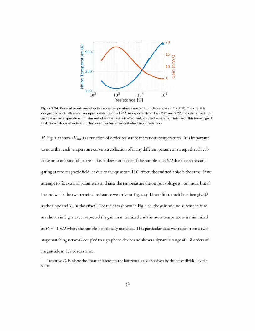
Figure 2.24: Generalize gain and effective noise temperature exracted from data shown in Fig. 2.23. The circuit is

designed to optimally match an input resistance of∼1kΩ. As expected from Eqn. 2.26 and 2.27, the gain is maximized

and the noise temperature is minimizedwhen the device is effectively coupled— i.e. Γ is minimized. This two-stage LC

tank circuit shows effective coupling over 3 orders of magnitude of input resistance.

R. Fig. 2.22 shows Vout as a function of device resistance for various temperatures. It is important

to note that each temperature curve is a collection of many different parameter sweeps that all col-

lapse onto one smooth curve — i.e. it does not matter if the sample is 13 kΩ due to electrostatic

gating at zero magnetic field, or due to the quantum Hall effect, the emitted noise is the same. If we

attempt to fix external parameters and raise the temperature the output voltage is nonlinear, but if

instead we fix the two-terminal resistance we arrive at Fig. 2.23. Linear fits to each line then give G

as the slope and Tn as the offset†. For the data shown in Fig. 2.23, the gain and noise temperature

are shown in Fig. 2.24; as expected the gain in maximized and the noise temperature is minimized

atR ∼ 1 kΩ where the sample is optimally matched. This particular data was taken from a two-

stage matching network coupled to a graphene device and shows a dynamic range of∼3 orders of

magnitude in device resistance.

†negative Tn is where the linear fit intercepts the horizontal axis; also given by the offset divided by theslope

36

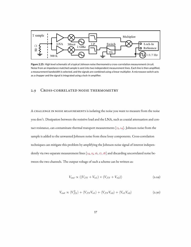
Figure 2.25: High level schematic of a typical Johnson noise thermometry cross-correlationmeasurement circuit.

Noise from an impedancematched sample is sent into two independent measurement lines. Each line is then amplified,

a measurement bandwidth is selected, and the signals are combined using a linear multiplier. Amicrowave switch acts

as a chopper and the signal is integrated using a lock-in amplifier.

2.9 Cross-correlated noise thermometry

A challenge in noise measurements is isolating the noise you want to measure from the noise

you don’t. Dissipation between the resistive load and the LNA, such as coaxial attenuation and con-

tact resistance, can contaminate thermal transport measurements [13, 14]. Johnson noise from the

sample is added to the unwanted Johnson noise from these lossy components. Cross-correlation

techniques can mitigate this problem by amplifying the Johnson noise signal of interest indepen-

dently via two separate measurement lines [14, 15, 16, 17, 18] and discarding uncorrelated noise be-

tween the two channels. The output voltage of such a scheme can be written as:

Vout ∝ ⟨(VJN + Vn1)× (VJN + Vn2)⟩ (2.29)

Vout ∝ ⟨V 2JN ⟩+ ⟨VJNVn1⟩+ ⟨VJNVn2⟩+ ⟨Vn1Vn2⟩ (2.30)

37

Figure 2.26: Auto- and cross-correlation Johnson noisemeasurements of a 50Ω resistor measured by the circuit

shown in Figs. 2.2 and 2.25, respectively. Inset shows the raw output voltage. The signal is converted to noise power

by the Nyquist equation. The solid lines are linear fits, where the auto- and cross-correlation data exhibit an offset of

68K and 2.6K , respectively, due to amplifier noise

where VJN is the instantaneous Johnson noise voltage and Vn1 and Vn2 are the instantaneous

voltage noise on the two channels. If all noise sources are uncorrelated then only the first term in

Eqn. 2.30 is non zero and Vout ∝ ⟨V 2JN ⟩.

Previously, cross-correlation measurements were limited to frequencies below a few MHz due to

the practical implementation of multipliers and digital processing speeds [17, 18, 19, 15]. However,

the 2GHz analog multiplier (Analog Devices ADL5931) and LNA, combined with the lock-in am-

plifier modulation scheme described in Fig. 2.25, measure the correlated noise between the two chan-

nels, rejecting a large portion of the uncorrelated amplifier noise. The results are shown alongside an

autocorrelation measurement (Fig. 2.2) for comparison in Fig. 2.26; the offset due to amplifier noise

was reduced from 68K to 2.6K .

38

Figure 2.27: Standard deviation of 1000 auto- and cross-correlation temperaturemeasurements as a function of inte-

gration time for 328MHz (left) and 28MHz (right). In all cases, uncertainty follows the Dicke relation, Eqn. 2.15,

scaling as√τ and

√∆f . Data is taken from a 50Ω resistor

Although the offset in the data is reduced by cross-correlation, the measurement time required to

achieve a given precision is not reduced†. The time required to effectively average out the uncorre-

lated noise is still proportional to the amplifiers noise temperature. To be precise, Tn is given by the

geometric mean of individual amplifiers noise temperatures.

Tn =√Tn1Tn2 (2.31)

where Tn1 and Tn2 are the system noise temperatures of the two measurement lines. Using two

LNAs with similar specifications Eqn. 2.31 reduces to the Dicke formula, Eqn. 2.15. Fig. 2.27 illus-

trates this point by showing the standard deviation of 1000 temperature measurements as a func-

†Cross-correlation can improve the accuracy of an experiment but not the precision

39

Figure 2.28: Cartoon of a four-terminal device. If the voltage between terminals A and C is cross-correlated to the

voltage between terminals B andD, the result will bemore sensitive to the temperature of the device than pairing A-B

and C-D

tion of integration time. Both auto- and cross-correlation measurements follow the Dicke formula

with similar magnitude and uncertainty scaling as√τ and

√∆f .

2.9.1 multi-terminal cross-correlation

Cross-correlation can be used to reduce the effects of contact and lead resistance with the

use of multi-terminal devices. However, as discussed in section 2.2, the voltage fluctuations on dif-

ferent pairs of terminals generally measure different areas of a device. For example, the four-terminal

device drawn in Fig. 2.28 will give very different results depending on which terminal are paired

— cross-correlation between VAC and VBD will by more sensitive to the device temperature than

cross-correlation of VAB and VCD. The exact amount of overlap between the noise on any pair of

terminals can be found via the method described in section 2.2.

40

3Electronic cooling mechanisms in graphene

Charge carriers in conductors exchange energy with the environment in many ways. If an

electronic system is directly heated — whether it be by Joule heating, optical pumping, or any other

direct energy transfer — the mechanisms with which the system cools can be quite diverse. In meso-

scopic samples there are typically three cooling mechanisms one has to consider. Firstly, if the ma-

41

terial is electrically connected to a thermal bath, such as macroscopic electrodes, then hot electrons

can diffuse out and cold electrons can diffuse in; this diffusion is often referred to as Wiedemann-

Franz cooling and is the dominate thermal transport mechanism in metals at low temperatures [20].

Secondly, hot electrons can transfer energy directly to the lattice by coupling to acoustic and optical

phonon modes in the graphene itself or the nearby substrate (section: 3.2). Thirdly, electrons are

charged and can therefore radiatively cool; this radiation is primarily in the form of Johnson noise

and, although often negligible, can be the dominate cooling mechanism in ultralow temperature

systems coupled to superconducting leads [21, 22].

3.1 Wiedemann-Franz

If a material hosts mobile charge carriers at a fixed temperature, each quasiparticle can

transport a quantized amount of thermal energy and a quantized charge through the system; it then

stands to reason that the electronic thermal conductivity must be related to the electrical conduc-

tivity. First observed at room temperature in 1853 by Wiedemann and Franz [23], the electronic

thermal conductivity (κ) of metals is directly proportional to the electrical conductivity (σ) at room

temperature. Twenty years later, Lorenz expanded upon the idea [24] and showed the ratio of the

thermal conductivity to the product of the electrical conductivity and temperature (T ) was a con-

stant,L.

κ

σT= L (3.1)

42

Figure 3.1: Experimental Lorenz number of elemental metals and degenerate semiconductors at low temperatures.

Taken from ref [25], reprinted with permission from Springer, license number 4067330556225

Eqn. 3.1 is now known as the Wiedemann-Franz law (WFL) whereL is the Lorenz ratio (also known

as the Lorenz number). Fig. 3.1 shows experimentally measured Lorenz numbers for various metals

and semiconductors as a function of conductivity and carrier concentration. The quantitative value

forL can be approximated under the Drude model [20] but it was not until Sommerfeld in 1927

that a full derivation using Fermi-Dirac statistics was presented [26]. Under the assumptions of

a degenerate Fermi gas and only elastic collisions, the theoretical value of the Lorenz number was

shown to be:

L0 ≡π2

3

k2Be2

≈ 2.44× 10−8 WΩ/K2 (3.2)

The requirement that quasiparticles only scatter elastically leads the value ofL to deviate fromL0 in

the presence of strong electron-electron scattering and inelastic electron-phonon scattering.

43

3.1.1 Linearization

To understand the behavior of devices under low energy excitations, it is useful to linearize

the WFL. In the linear response regime the temperature variations across a device are small com-

pared to the absolute temperature scale of the problem, Tb. For a uniform two-dimensional device

connecting two thermal baths with temperatures Tb ±∆T/2, the steady state thermal power trans-

ported via the WFL is given by:

QWF =

(Wσ

L

)LTb ∆T =

LTb

R∆T (3.3)

where W and L are the sample width and length, respectively, and R is the two-terminal electrical

resistance

3.1.2 Hot-electron shot noise

A common way to develop a temperature gradient is via Joule heating, where the electron

temperature is raised with reference to the cold electrodes held at Tb. In the case of only WF conduc-

tion — i.e. no alternative cooling pathways such as phonons — the temperature rise in the high bias

regime scales linear with the applied current, producing noise very similar to the shot noise seen in

vacuum tubes. This well known effect is termed “hot-electron shot noise” [27, 28, 29] and can be

44

seen as the limit of the WFL with Te >> Tb.

Q ≈ βLR

T 2e (3.4)

where β is a constant related to the temperature profile in the device. If we set the power dissipated

to be proportional to the current squared, such that Q = I2R, we find:

⟨Te⟩ ≈R√βL

I (3.5)

Solving for the temperature profile and the noise produced, eqn. 3.5 reduces to [27]:

SI =

√3

42e I (3.6)

Eqn.3.6 has the same form as shot noise with Fano factor of√3/4.

3.2 Electron-Phonon coupling

At higher temperatures, the cooling of hot electrons is dominated by coupling to acoustic

and optical phonons in the hexagonal lattice as well as the nearby substrate [30, 31]. In many experi-

ments involving optical heating or Joule heating, a quasi-equilibrium can be formed where the elec-

tron temperature and the lattice temperature can be different. In the particular case of monolayer

45

graphene this is especially true as the high phonon conductivity and relatively weak electron-phonon

coupling can result in a lattice temperature that is well thermalized to the thermal bath (Tb), but

an electron temperature (Te) which is not. The interaction between these fermionic and bosonic

systems in graphene is quite rich with even the power law for the temperature dependence varying

depending on the Fermi level, device disorder, and bias voltage. A general form for the heat transfer

between the two systems can written as:

Qe−ph = AΣe−ph

(T δe − T δ

b

)(3.7)

where A is the area of the device,Σe−ph is a coupling constant, and δ is the is the power law expo-

nent. Depending on the mechanism δ can vary between 3 [32, 33] in disordered samples, or 4− 5 in

clean devices [30, 31]. These relatively high power laws result in phonons dominating at high temper-

ature but becoming negligible when cold.

3.2.1 Linearization

To find the linear response behavior (∆T ≪ Tb) we can Taylor expand to first order for

Te ≈ Tb to find:

Qe−ph ≈ A δ Σe−phTδ−1

b ∆T (3.8)

Eqn. 3.8 can be compared directly to eqn. 3.3. First we see that while both cooling mechanisms scale

as the device width, they have inverse dependences on the device length and, therefore, the bath

46

temperature at which one mechanism will dominate over the other is geometry dependent.

The literature on electron-phonon coupling in graphene is vast [34, 35, 30, 31, 36]. Here I present

a condensed review of the main mechanisms relevant to the experiments presented in this disserta-

tion.

3.2.2 Bloch-Gruneisen temperature

In most three-dimensional metals, where the Fermi surface is large, the characteristic tem-

perature scale for phonon dynamics is given by the Debye temperature. However, in semiconduc-

tors and semimetals the Fermi surface can be substantially smaller than the Brillouin zone leading

to a second temperature scale which governs the scattering of electrons and phonons. The Bloch-

Grüneisen temperature, TBG, is the temperature at which the most energetic phonons have a typical

momentum equal to the Fermi momentum[37, 38].

TBG =2ℏvskFkB

(3.9)

Above this temperature, momentum conservation dictates that only a fraction of the available

phonon modes can scatter electrons. This is because the largest momentum change an electron can

experience is 2kF — a complete backscatter — and, as such, only phonons with momentum equal

to or less than 2kF can participate in scattering processes. This has been shown in GaAs based 2D

electron systems [39] and in graphene [40] where TBG can be controlled by tuning the Fermi level

47

using an electrostatic gate.

3.2.3 Acoustic phonons

In typical metals at low temperature, the dominate phonon modes in the system are acous-

tic [20]†. In graphene, however, energy transfer between electrons and these acoustic phonons (AP)

is limited by the mismatch between the Fermi velocity (vF ) and the sound speed in the material (vs).

Energy and momentum conservation limit the energy that each phonon collision can remove from

the electronic system, resulting a maximal energy transfer of 2ℏvskF per collision. Nevertheless, ex-

periments have shown that the electronic cooling in many graphene devices at low temperatures is

dominated by AP scattering [41, 42, 43] .

Theoretical predictions for the the power law δ and the coupling constantΣe−ph have been

shown to depend upon the device temperature and the amount of disorder. In the dirty limit, the

energy and momentum conservation discussed above can be circumvented by disorder-assisted colli-

sions called “supercollisions” resulting in a power law δ = 3 [32]. In the clean limit at low tempera-

ture, Kubakaddi [44] showed δ = 4with a coupling constant:

Σe−ap =π2D2|µ|k4B15ρℏ5v3F v3s

(3.10)

whereD is the deformation potential, µ is the chemical potential, and ρ is the mass density of the

†The optical phonon branch has finite energy at k = 0 and thus at low enough temperatures these modesare frozen out

48

Figure 3.2: Numerical calculations of the thermal conductance between graphene electrons and acoustic phonons

as a function of temperature normalized to the chemical potential (µ). the thermal conductanceG scales asT δ−1.

G0 ∝ µ4 is a temperature independent normalization constant. For temperatures belowTBG the electron-phonon

power law δ scale asT 4 while at high temperature Viljas et al. find δ ∼ T 5. Reprinted with permission fromRef. [30]

by the American Physical Society license number: 4077361227141.

lattice. Eqn. 3.10 was reproduced by Viljas et al. [30] and extended to high temperature where it was

found that δ approaches 5. The transition from these two regimes is shown in fig. 3.2.

3.2.4 Optical phonons

Although the energies associated with optical phonons in graphene are quite large

compared to the thermal energies in typical low temperature experiments, each collision can re-

move a significant amount of energy from the electronic system. Bistritzer et al. [31] showed that,

at sufficiently high temperatures, even the∼200meV graphene intrinsic optical phonons can dom-

inate the electronic cooling in suspended samples. For encapsulated devices, remote phonons in the

49

boron-nitride have been shown to have a surprisingly significant effect both theoretically [30, 31, 45]

and experimentally [35]. At higher temperature (≳ 270K), Sohier et al. [34] showed that despite

the relatively low occupancy, graphene intrinsic optical phonons can have a more pronounced effect

on the electrical resistance than acoustic phonons.

3.3 Photon cooling

For a device coupled to a microwave circuit, energy is radiated via photons over the mea-

surement bandwidth [46, 47]. This is equivalent to 1D blackbody radiation and is the noise which

is measured in Johnson noise thermometry. The power transferred is given by eqn. 2.13 and is con-

sidered to be negligible compared with the Wiedemann-Franz and phonon cooling powers for the

temperatures and bandwidths covered in this dissertation. However, for devices at low temperature

with superconducting leads this can become a significant source of cooling [47].

3.4 Thermal Network

When heat is injected into the electronic system of graphene, each of the mecha-

nisms described above plays a role in thermalizing the system to an external bath. For the devices

and experimental parameters used in this dissertation, a simplified thermal model can be used (il-

lustrated in fig. 3.3). The electronic system is connected to the bath by two parallel cooling paths: a

50

Figure 3.3: A thermal model of the electronic cooling pathways in graphene. Heat injected into the electronic system

can flow directly to the bath viaWiedemann-Franz conduction, or to the lattice via electron-phonon coupling. The

lattice and the bath are connected via the lattice conductivity which is large in graphene.

51

diffusion channel and a lattice channel. The diffusion channel is governed by the electronic ther-

mal conductivity, while the lattice channel contains both an electron-phonon coupling term and

the lattice conductivity of graphene. In practice the lattice conductance is typically many orders of

magnitude larger than the electron-phonon conductance† resulting in the lattice being well sunk to

the bath [10, 41, 48]. The temperature dependence of the two channels follow different power laws

resulting in the low temperature behavior being governed by diffusive conduction while cooling at

high temperatures is dominated by the lattice channel.

†The ratio of the lattice conductance to the electron-phonon conductance is geometry dependent. In longsamples the phonon conductance may bottleneck the lattice cooling channel.

52

Since the dawn of time, man hath sought to make things

smaller.

4Thermal conductance via electrical noise

A common technique in studying the various cooling pathways in a mesoscopic sample is to in-

ject a pulse of energy into the system and monitor the time dependent electron temperature as the

system returns to equilibrium. However, these “pump-probe” experiments suffer from a few diffi-

culties: Firstly, they yield a thermal time constant which is a convolution of the various heat capaci-

53

ties and thermal conductances in the problem. Secondly, the large temperature rise needed to resolve

the thermal decay makes it difficult to study the linear response of low energy excitations. A steady

state experiment avoids these difficulties and enables the measurement of thermal conductance in

linear response at the expense of time-resolution.

In a steady state thermal experiment, a constant heating power, P0, is injected into the electronic

system and the electron temperature rise,∆T , is measured. For the experiments in this dissertation,

this is accomplished via Joule heating in a two terminal geometry while monitoring the change in

Johnson noise temperature, TJN — as discussed in chapter 2.2. We can define the ratio of the ap-

plied power to the change in the Johnson noise temperature as a thermal conductance:

Gth =P0

∆TJN(4.1)

It is important to note thatGth is not the traditional thermal conductance which describes the total

heat power flowing through a material in response to a spatial temperature gradient; it is instead a

generalized thermal conductance describing the heat power transferred between the electronic sys-

tem and the bath under Joule heating. To extract meaningful microscopic parameters fromGth it is

necessary to model how the heat is entering and leaving the system as a function of these parameters.

For the devices and experimental parameters presented here, the simplified thermal model shown in

fig. 4.1 can be used to extract information about the electronic thermal conductivity and the electron-

phonon coupling.

54

Figure 4.1: Simplified thermal diagram of the electronic cooling pathways in graphene relevant for the experimental

conditions presented here. A current induces a heating power into the electronic systemwhich conducts to the bath

via two parallel pathways: diffusion and coupling to phonons.

4.1 Rectangular devices

For a two-terminal rectangular device, the temperature measured by Johnson noise —

as given by Eqn. 2.12 with spatially uniformP(r)— is simply the spatially averaged temperature.

Therefore, the total thermal power dissipated in linear response is then given by:

I2R = P0 = Q =

(W

Lβκ+WLΣe−phδT

δ−1b

)∆TJN (4.2)

whereW andL are the sample width and length, respectively, Tb is the bath temperature, κ is the

electronic thermal conductivity,Σe−ph and δ are the electron-phonon parameters described in

Ch. 3.2, and∆TJN is the Johnson noise temperature minus the bath temperature. In Eqn. 4.2 we

have used the steady-state requirement that the total heating power entering the system equal the

55

total power transferred to the bath (P0 = Q). The geometric factor β depends on the shape of the

electronic temperature profile which is affected by the relative strength of the two cooling terms in

Eqn. 4.2 and must be calculated.

4.1.1 Electronic conduction only

In the absence of phonons, the temperature profile, and therefore β, can be solved analyti-

cally. In a rectangular geometry, symmetry reduces the problem to one dimension (x) along the

source-drain direction. For simplicity we assume that the graphene sample is homogeneous, that the

approximately uniform electrical current is given by

J = −σdVdx

− αdTdx

(4.3)

and that the heat current is given by

q = −αTdVdx

− κdTdx

(4.4)

where dT/dx is the temperature gradient in the sample,−dV/dx is the electric field in the sample,

and α/σ is the Seebeck coefficient. From Eqn. 4.3 we see that the electrical conductivity, which is de-

fined as the relation between the electric current and a potential gradient in the absence of a thermal

gradient, is simply given by σ. Unfortunately, the thermal conductivity (κ) is not symmetrically de-

56

fined as the relation between the heat current and the thermal gradient in the absence of a potential

gradient, but instead as the relation between q and dT/dx in the absence of a charge current J . We

therefore find:

κ ≡ κ+Tα2

σ= κ (1 + ZT ). (4.5)

In the latter equation,ZT is the thermoelectric coefficient of merit. In the limit of negligible thermo

electric effects κ ≈ κ.

The continuity equation for the electric current yields:

0 =dJdx

(4.6)

In the linear response regime, the Joule power per unit length,P , is given by J · E and thus the

continuity equation for the heat current with a source term becomes:

P =J2

σ=

dqdx

(4.7)

combining the above equations we obtain

P = −κd2Tdx2

(4.8)

assuming that κ is approximately homogeneous throughout the sample.

57

The contacts serve as thermal baths and thus are held at the same temperature Tb. Writing

T (x) = Tb +∆T (x) (4.9)

and solving Eqn. 4.8 using this form for the solution with the boundary conditions∆T (0) =

∆T (L) = 0we find a parabolic temperature profile:

∆T (x) =P2κ

x(L− x) (4.10)

The average temperature change in the sample, which is directly measured through Johnson noise

thermometry, is

∆TJN = ⟨∆T ⟩ =L∫

0

dxL

∆T (x) =PL2

12κ(4.11)

Plugging in the power per unit lengthP in terms of σ and the external voltage V0 yields:

∆TJN =V 20 σ

12 κ(4.12)

We find∆TJN to be independent of the sample dimensions. This non-uniform temperature profile

is illustrated in Fig. 4.2.

Combining Eqs. 4.2 and 4.11, we obtain the relation between the experimentally measuredGth

58

Figure 4.2: Cartoon illustrating the non-uniform temperature profile within the graphene-hBN stack during Joule

heating in the diffusion-limited regime.

and the microscopic quantity of interest κ as:

Gth ≡ P0

∆TJN=

12W

Lκ (4.13)

All the information about the heating profile is contained in the constant factor of 12. — i.e for

a two-terminal rectangular geometry under Joule heating β = 12. If the electronic conductance

follows the Wiedemann-Franz law, such that κ = LσT , then Eqn. 4.13 becomes

Gth =12WLσTb

L=

12LTb

R(4.14)

where R is the directly measurable, two-terminal electrical resistance.

4.1.2 Phonon cooling only

The limit of electron-phonon dominated cooling can be modeled by phonons effectively

removing an isotropic amount of heat per unit area; the balance between this and Joule heating leads

59

to a uniform temperature profile,

∆T (x) = T0 = ∆TJN (4.15)

The heat balance equation (Eqn. 4.2) then becomes

I2R = WLΣe−phδTδ−1b ∆TJN (4.16)

and thus the microscopic parameters governing electron-phonon coupling are related to the experi-

mentally measured thermal conductance in the linear response regime by

Gth = WLΣe−phδTδ−1b (4.17)

4.2 Wedge devices

Unlike in rectangular devices, where the Johnson noise temperature is simply the mean

temperature, in more complicated geometries the effective temperature measured in a noise exper-

iment must be calculated from the Joule heating temperature profile. An instructive example of a

more complicated geometry which can also be solved analytically is a semicircular wedge as shown in

fig. 4.3. The continuity equations for charge current in cylindrical coordinates yield

60

Figure 4.3: Sketch of a wedge shaped device and boundary conditions for Joule heating. Red boundaries representcontacts where temperature is fixed atTb. A voltageV0 is placed on the contact at r = r1 while the second contact atr = r2 is held at ground. Cylindrical symmetry leaves heat and charge currents independent of angle.

J(r) = − V0 σ

ln(r1/r2)1

rr (4.18)

and for heat current with a Joule heating source term

J2

σ= ∇ · q = κ

d2Tdr2

+κ

r

dTdr

(4.19)

Combining Eqns. 4.18 and 4.19 and solving using the thermal boundary conditions of fixed tempera-

ture at the contacts, the temperature profile is given by:

∆T (r) =V 20 σ

2κ ln (r1/r2)2ln(

r

r1

)ln(

r

r2

)(4.20)

61

The mean temperature and the Johnson noise temperature can be calculated by integrating Eqn.

4.20 yielding,

⟨∆T ⟩ =r2∫

r1

T (r) r dr/ r2∫

r1

r dr

=V 20 σ

4 κ ln(r2/r1)

[r11 + r22r11 + r22

− ln(r2/r1)]

(4.21)

∆TJN =

r2∫r1

q(r)T (r) r dr/ r2∫

r1

q(r) r dr

=V 20 σ

12 κ(4.22)

The difference between the spatially averaged temperature and∆TJN illustrates the power of com-

bining Joule heating with Johnson noise thermometry — the spatial distribution with which heat

is injected into the system is the same as the spatial weighting function for Johnson noise measure-

ments. Rewriting Eqn. 4.22 in terms ofGth assuming the Wiedemann-Franz law we arrive at the

same form as Eqn. 4.14,

Gth =12LTb

R(4.23)

All geometric dependence is contained in the experimentally measurable two-terminal resistanceR

and we find, similar to the rectangular geometry, β = 12.

62

4.3 Universality of β

Above we have derived two analytic examples where β was shown to be 12. In fact, it can

be shown that β = 12 is universally true in the linear response regime regardless of the geometry of

the device or the form of the conductivity tensors, σ and κ, provided the following conditions are

met:

1. The device has only two electrical terminals which serve as thermal heat sinks and sources ofJoule heating current

2. Electron cool is provided only by Wiedemann-Franz diffusion

3. σ and κ are spatially uniform

4. The elastic mean free path of the charge carriers is shorter than all other relevant length scalesin the system

The following derivation is adapted from a work done by Dr. Brian Skinner, MIT, altered for

clarity and brevity:

Without loss of generality, we can imagine a unit voltage applied across an arbitrary two terminal

device, so that the electric potential ϕ(r) has ϕ = 1 at the source electrode and ϕ = 0 at the drain.

For a generic conductivity tensor σ (which may be affected by magnetic field) the electric current

J(r) is

J(r) = −σ∇ϕ. (4.24)

63

Thus, the continuity equation ∇ · J = 0 becomes

∇ · σ∇ϕ = 0 (4.25)

This equation, together with the boundary conditions, defines the electric potential. The bound-

aries at non-contact edges are assumed to be reflecting, so that (∇ϕ) · n = 0, where n is a unit

normal vector to the boundary.

The electron temperature T (r), defined relative to the bath temperature Tb, obeys the heat diffu-

sion equation

P(r) = −∇ · (κ∇T ), (4.26)

if there are no extraneous sources of heat dissipation, such as electron-phonon coupling, then the

steady state condition will setP equal to the dissipated Joule heating power per unit area. The Joule

power is given by J · E, or

P(r) = (σ∇ϕ) · (∇ϕ) (4.27)

If we assume the generalized Wiedemann-Franz relation in the linear response regime, κ = σLTb,

we arrive at the following relation governing the temperature:

(σ∇ϕ) · (∇ϕ) = −LTb∇ · (σ∇T ). (4.28)

Together with the boundary conditions, this equation defines the temperature profile T (r). We

64

assume that the contacts are good heat sinks, so that T = 0 at both contacts, and that no heat is lost

at the boundary of the sample: (∇T ) · n = 0.

Eqn. 4.28 makes clear that there is a close relation between the temperature profile and the electric

potential. It can be shown that Eqn. 4.28 and the boundary condictions are satisfied by the ansatz,

T (r) =1

2L Tbϕ(r)(1− ϕ(r)). (4.29)

From Eqn. 4.29 we can calculate the Johnson noise temperature via Eqn. 2.12:

∆TJN =

∫d2rP(r) T (r)

P0

=R

2LTb

∫d2rϕ(r) [1− ϕ(r)]

[σ∇ϕ(r)

]·[∇ϕ(r)

](4.30)

Here we have used P0 = V 2/R = 1/R (assuming our voltage units). Combining Eqn. 4.29 and

4.30 we can write∆TJN is terms of only the temperature profile:

∆TJN = LTbR

∫d2rT (r)∇ · (σ∇T )

= LTbR

∫d2r(∇T (r)) · (σ∇T (r)). (4.31)

Eqn. 4.31 was found using integration by parts, and noting that either T or ∇T vanishes at the

boundaries of the sample.

65

The geometric factor β is defined by

1

β≡ ∆TJN L Tb

QR. (4.32)

Plugging in Eqn. 4.30

1

β=

1

2 P0

∫d2rϕ(1− ϕ)(σ∇ϕ) · (∇ϕ). (4.33)

On the other hand, inserting Eqn. 4.29 into eqn. 4.31 and rearranging gives

1

β=

1

4 P0

∫d2r

[∇(ϕ(1− ϕ))

]·[σ∇(ϕ(1− ϕ))

]=

1

4 P0

∫d2r(1− 2ϕ)2(∇ϕ) · (σ∇ϕ)

=1

4 P0

[∫d2r(∇ϕ) · (σ∇ϕ)−

∫d2r 4ϕ(1− ϕ)(∇ϕ) · (σ∇ϕ)

]. (4.34)

The second term in Eqn. 4.34 is identical to the right hand side of Eqn. 4.33 multiplied by 2, and it is

therefore equal to 2/β. Thus:

1

β=

1

4 P0

∫d2r(∇ϕ) · (σ∇ϕ)

=1

12 P0

∫d2r(∇ϕ) · (σ∇ϕ)

=1

12 P0

∫d2r P(r) (4.35)

The final step in Eqn. 4.35 comes from realizing the integrand is simply the Joule heating power

66

Figure 4.4: Simplified schematic of thermal conductancemeasurement setup. A low frequency Joule heating current

is pass through the sample using a lock-in amplifier and the corresponding temperature is measured using Johnson

noise thermometry. A bias tee is used to combine the DC and RF signals. The noise signal is measured as the second

harmonic of the heating current as∆T ∼ I2

given in eqn. 4.27, and thus

β = 12 (4.36)

4.4 Experimental setup

To sensitively measure∆TJN , the autocorrelation Johnson noise thermometry circuit de-

scribed in chapter 2 can be modified to allow a DC current to Joule heat the sample. Fig. 4.4 shows

a simplified schematic of a thermal conductance measurement setup. A low frequency (f∼ 13Hz)

current is generated by a lock-in amplifier† at frequency ω = 2π×f and passed through the sample‡

using a bias tee. If the current is given by:

I(t) = I0 sin(ωt) (4.37)

†This lock-in is also used to measure the two-terminal resistanceR‡It is because of this need to pass a DC current through the matching network and into the sample that

the LC tanks used are setup in a low-pass configuration

67

Figure 4.5: Electron temperature of a two-terminal graphene device (inset) as a function of a Joule heating currentfor three different bath temperatures. The temperatures follow an I2 heating lawwith the curvature determined by

the generalized thermal conductanceGth which increases with the bath temperature. Here electron temperature is

defined as the Johnson noise temperature as discussed in section 4.1

the total heating power dissipated in the device is

P0(t) = I20R sin2(ωt) (4.38)

and the corresponding temperature rise in Johnson noise temperature is

∆TJN (t) =I20R

Gthsin2(ω t)

=I20R

2Gth(1− cos(2 ω t)) (4.39)

The 2ω component of the corresponding noise signal is then measured by a second lock-in ampli-

fier detecting the second harmonic of the Joule heating current (phase shifted by π/2) as shown in

Fig. 4.4.

68

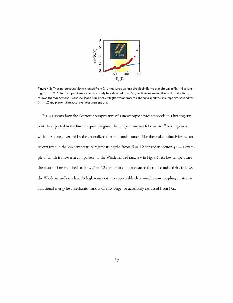
Figure 4.6: Thermal conductivity extracted fromGth measured using a circuit similar to that shown in Fig. 4.4 assum-

ingβ = 12. At low temperatureκ can accurately be extracted fromGth and themeasured thermal conductivity

follows theWiedemann-Franz law (solid blue line). At higher temperatures phonons spoil the assumptions needed for

β = 12 and prevent the accuratemeasurement ofκ

Fig. 4.5 shows how the electronic temperature of a mesoscopic device responds to a heating cur-

rent. As expected in the linear response regime, the temperature rise follows an I2 heating curve

with curvature governed by the generalized thermal conductance. The thermal conductivity, κ, can

be extracted in the low temperature regime using the factor β = 12 derived in section 4.1 — a exam-

ple of which is shown in comparison to the Wiedemann-Franz law in Fig. 4.6. At low temperature

the assumptions required to show β = 12 are met and the measured thermal conductivity follows

the Wiedemann-Franz law. At high temperatures appreciable electron-phonon coupling creates an

additional energy loss mechanism and κ can no longer be accurately extracted fromGth.

69

5Thermal conductance in high density

graphene

When the Fermi level of graphene is doped far from the Dirac point (µ ≫ kBT ), graphene

has a well defined Fermi surface and the assumptions in Sommerfeld’s derivation of the Lorenz ra-

70

Figure 5.1: (le ) Device image and (center) electronic thermal conductivity of graphene on SiO2 measured by Fong

et al. [41] using Johnson noise thermometry. Dashed line is a fit to theWiedemann-Franz law. Below 1K the device

showsWF behavior while at higher temperature themeasured conduction is higher due to phonons coupling. The

longer device used in this study resulted in phonons dominating conductance at a lower temperature. (right) Thecorrespondingmeasured Lorenz ratio vs carrier density. Reprinted under the Creative Commons Attribution 3.0

License fromRef. [41].

tio hold. In 2013, Fong et al. [41] verified the Wiedemann-Franz for graphene on SiO2 (Fig. 5.1) us-

ing Joule heating and Johnson noise thermometry. The device measured had a mobility of µ ≳

5, 000 cm2/V s and a length which emphasized phonon scattering, resulting in the Wiedemann-

Franz law (WFL) only being verifiable until 1K . Nevertheless, a Lorenz ratio varying between

1 − 2L0 was measured for various charge densities (Fig. 5.1) at low temperature. Above 1K the

thermal conductance increased above the WFL due to electron-phonon scattering as described in

section 3.2. A few months later, Yigen et al. [49] performed similar Joule heating experiments us-

ing resistive thermometry with higher quality suspended graphene (µ ≳ 35, 000 cm2/V s). As

shown in Fig.5.2, the shorter device geometry allowed them to measure the WFL to a much higher

temperature of∼150K finding experimental Lorenz ratios of about 0.5L0.

In this chapter we present similar data on higher mobility samples encapsulated with hexagonal

71

Figure 5.2: Electronic thermal conductivity of suspended graphenemeasured by Yigen et al. [49] using resistive ther-

mometry. Two curves correspond to different carrier densities. Solid lines are fits to theWiedemann-Franz law. Below

∼ 150K the device shownWF behavior while at higher temperature themeasured conduction is higher due to

phonons coupling. Device is 650nm long. Reprinted with permission from [49]. Copyright (2014) American Chemical

Society.

boron nitride (hBN).

5.1 Device characteristics

Monolayer graphene is mechanically exfoliated, encapsulated in hexagonal boron ni-

tride, and contacted along its 1-dimensional edge [50] to form a (2 µm × 6 µm) channel (Fig. 5.3).

A typical two-terminal channel resistanceR of this device varies between 150 and 800Ω depending

on the back gate voltage. The mobility, µ, of the device can be estimated by fitting the two-terminal

resistance as a function of charge density n, as shown in Fig. 5.3, to find µ ≈ 330, 000 cm2/V s at

3K and µ ≈ 60, 000 cm2/V s at 300K .

As maximal noise power is collected when the device is impedance matched to the measurement

chain, an LC tank circuit is placed on chip to transform the graphene to 50Ω (as disscussed in sec-

72

Figure 5.3: (le ) Microscope image of the two-terminal graphene device (2µm× 6µm) used in thermal conduction

studies presented in this chapter. (right) Estimated resistivity vs carrier density from two-terminal resistance. Solid red

line is a fit used to estimate a carrier mobility ofµ ≈ 330, 000 cm2/V s.

50 75 100 125 150 175 200−90

−80

−70

−60

−50

−40

−30−20

Frequency (MHz)

R = |S11|2 (dB)

LC

matching

network

5 mm

Figure 5.4: RF reflectance off the two-terminal graphene device presented in this chapter. The sample impedance is

transformed using a single stage LC network (inset) resulting in ameasurement bandwidth of 25MHz centered at

133MHz. See section 2.6 for details on impedancematching.

tion 2.6 and Refs. [51] and [52]) within the measurement bandwidth. The matching network de-

fines a bandwidth of 25MHz centered at 133MHz, as shown in Fig. 5.4. The total noise power

emitted into this bandwidth is amplified and measured via the circuit and procedure outlined in

chapter 4 resulting in a measured output voltage (proportional to the total noise power) similar to

that shown in Fig. 5.5

73

−10 −5 0 50

50

100

150

200

250

300

Gate Voltage [V]

Ba

th T

em

pe

ratu

re [

K]

100

140

180

220

260

µV

Figure 5.5: MeasuredDC voltage proportional to the total noise emitted from a graphene device as a function of bath

temperature and back gate voltage using the circuit outline in chapter 2.

5.2 Thermal conductance

For the results shown here, the graphene device is measured away from the charge neutrality

point with hole density n ≈ 5.7 × 1010cm−2, whereR varies between 280 and 480Ω from 3

to 300K . The Johnson noise thermometer is calibrated to a given sample following the procedure

outlined in chapter 2 and the thermal conductance,Gth, is extracted as discussed in chapter 4.

The thermal conductance of our device falls into two temperature regimes as shown in Fig. 5.6.

For T < 100K ,Gth linearly depends on temperature and is well described by the Wiedemann-

Franz law. The dashed line in the left panel of Fig. 5.6 shows the theoretical Wiedemann-Franz con-

ductance (GWF ) with an offset of 0.015 µW/K . The fitted [41, 49] Lorenz number is 2.38 ×

10−8WΩK−2, 3% below the theoretical value. As the charge density is swept, the Lorenz ratio

74

Figure 5.6: (le ) Graphene thermal conductance from 3K to 300K . Blue dashed line shows the theoretical

Wiedemann-Franz conductance for our device geometry offset by a fitted constant. (Inset) shows the total conduc-tance withGWF subtracted. AboveT ∼ 80K , the conductance departs with a power law of 3.88 ± 0.02. (right)Same data with the fitted offset removed, shown on a log-log scale.

varies similar to that seen in ref [41], always remaining close toL0.

At higher temperature, the measuredGth is larger than Wiedemann-Franz conductance indi-

cating a different energy transfer mechanism dominates above 100K . Fig. 5.6(right) shows the

same data on a log-log plot making clear the two different power laws in the different regimes.

To extract the electron-phonon coupling constants, as outlined in section 3.2, the thermal con-

ductance from electron diffusion must be accounted for. Fig. 5.6 inset plotsGth withGWF sub-

tracted. Gth departs fromGWF with a fitted power law of 3.88 ± 0.02 and an amplitude of

0.23 ± 0.03 fW/K4.88. We note that the high power law δ ≈ 4 in our measured data is in

sharp contrast to the sublinear temperature dependence of graphene’s lattice conductivity for T >

150K [48], suggesting that it is unlikely the energy transfer bottleneck and hence the lattice is well

thermalized to the bath.

We compare the high temperature thermal conductance of our sample with the expected contri-

75

1 10 10010-10

10-9

10-8

10-7

10-6

Temperature (K)

Ther

mal

Con

duct

ance

(W/K

)

Wiedemann-Franzmeasured phonon coupling

supercollisionacoustic phonons

our data

Figure 5.7: Thermal conductance of a graphene device compared to estimated contributions from acoustic

phonons [31, 30] and the supercollision coolingmechanism [32, 33, 42, 43].

butions from acoustic phonons [31, 30] and the supercollision cooling mechanism [32, 33, 42, 43]

given the measured mobility in Fig. 5.7; We estimate these contributions to be an order of magni-

tude too small to explain the observedGth. From our experiment, we estimate that the thermal

conductance per unit area at 300K to be 9.5 × 104 W/Km2. We find this to be comparable to

theoretical calculations which suggest that optical phonons, both in the graphene lattice and the

boron nitride substrate, may provide an energy relaxation channel substantially larger than acoustic

phonons in this high temperature limit [34, 35, 30, 31, 36].

76

6The Dirac fluid

While the term “Fermi liquid” is often used to describe the electron flow in a metal, the key

feature of Fermi liquid theory is that the electron-electron interactions are renormalized away leav-

ing something more analogous to a non-interacting gas than an ordinary fluid, like water. In strongly

correlated systems, however, these interactions can dominate causing behavior ranging from Mott

77

insulators to high temperature superconductivity. In graphene near the charge neutrality point, a

unique situation occurs where quasi-relativistic electrons are holes coexist and interact. In the limit

of perfectly clean samples (and in the absence of phonon coupling), inter-particle scattering causes

dissipation to electrical currents as electron and holes are driven in opposite directions by an elec-

tric field. This effect has been notoriously difficult to observe as scattering off of impurities and

phonons can easily dominate inter-particle scattering in traditional graphene samples on SiO2. Even

in the case of clean samples, demonstrating that electron-electron scattering is dominate requires

a measurement that can distinguish between the momentum conserving inter-particle collisions

and the more traditional elastic scatting off impurities. One such measurement is to compare the

response of a device under an electric field to its response under a thermal gradient; while an electric

field drives electrons and holes in opposite directions, a thermal gradient drives them in the same

direction, therefore inter-particle scattering causes dissipation to electric current but not to heat

current (inset of Fig. 6.5c).

6.1 Temperature regimes

In general there are three primary scattering mechanism in graphene that can dom-

inate transport: impurities, inter-particle, and phonon. At low temperature, charge impurities in

graphene cause significant spatial variations in the local chemical potential resulting in what are

known as electron-hole puddles. Shown in Fig. 6.1 are scanning tunneling microscope images of

78

Figure 6.1: Spatial maps of the density of states of graphene on hBN and SiO2. a, Topography of graphene on hBN.b, Tip voltage at the Dirac point as a function of position for graphene on hBN. c, Tip voltage at the Dirac point as afunction of position for graphene on SiO2. The color scale is the same for b and c. The scale bar in all images is 10 nm.

dHistogram of the energies of the Dirac point from b as well as a Gaussian fit. The inset shows the same data but

also includes the histogram for SiO2 shown in red. Taken from ref [53], reprinted with permission from the Nature

Publishing Group license number 4082110543400

79

Figure 6.2: The interaction regime emerges in very clean samples. Taken fromD. Y. H. Ho et al. (in preparation, 2017)

with permission from S. Adam.

these puddles, taken for graphene on traditional SiO2 substrates and on hexagonal boron nitride

(hBN) [53]. On hBN these puddles can be of size> 100 nm— which is comparable to the electron-

electron scattering length at moderate temperatures — and have a potential variation with standard

deviation∼ 5meV . As temperature is increased, the effects of scattering off these charge impurities

lessens and, at high enough temperatures, phonon scattering becomes significant, as described in

section 3.2.

Whether there exists an intermediate temperature where inter-particle scattering becomes domi-

nate depends on the disorder level. D. Ho et al. [54] quantitatively compares the scattering rates in

graphene and finds that, for samples on hBN, a temperature window opens up where the electron-

electron scattering time becomes the fastest in the system, Fig. 6.2.

Using clean samples on hBN and the thermal techniques presented in the previous chapters, we

measured the electronic thermal conductivity of graphene at intermediate temperatures demonstrat-

80

ing that conduction is dominated by inter-particle scattering.

Below we present the original text of Ref. [55]. Reprinted with permission from J. Crossno, J.K.

Shi, K. Wang, X. Liu, A. Harzheim, A. Lucas, S. Sachdev, P. Kim, T. Taniguchi, K. Watanabe, T.A.

Ohki, and K.C. Fong. Science, 351(6277), pp.1058-1061 (2016). Copyright (2016) by AAAS.

6.2 Observation of the Dirac fluid and the breakdown of the

Wiedemann-Franz law in graphene

Understanding the dynamics of many interacting particles is a formidable task in

physics, complicated by many coupled degrees of freedom. For electronic transport in matter, strong

interactions can lead to a breakdown of the Fermi liquid (FL) paradigm of coherent quasiparticles

scattering off of impurities. In such situations, the complex microscopic dynamics can be coarse-

grained to a hydrodynamic description of momentum, energy, and charge transport on long length

and time scales [56]. Hydrodynamics has been successfully applied to a diverse array of interacting

quantum systems, from high mobility electrons in conductors [57], to cold atoms [58] and quark-

gluon plasmas [59]. As has been argued for strongly interacting massless Dirac fermions in graphene

at the charge-neutrality point (CNP) [60, 61, 62, 63], hydrodynamic effects are expected to greatly

modify transport coefficients as compared to their FL counterparts.

Many-body physics in graphene is interesting due to electron-hole symmetry and a linear disper-

sion relation at the CNP [64, 65]. In particular, the Fermi surface vanishes, leading to ineffective

81

screening [66] and the formation of a strongly-interacting quasi-relativistic electron-hole plasma,

known as a Dirac fluid [67]. The Dirac fluid shares many features with quantum critical systems

[68]: most importantly, the electron-electron scattering time is fast [69, 70, 71, 72], and well suited

to a hydrodynamic description. A number of exotic properties have been predicted including nearly

perfect (inviscid) flow [73] and a diverging thermal conductivity resulting in the breakdown of the

Wiedemann-Franz law [74, 61].

Away from the CNP, graphene has a sharp Fermi surface and the standard Fermi liquid (FL) phe-

nomenology holds. By tuning the chemical potential, we may measure thermal and electrical con-

ductivity in both the Dirac fluid (DF) and the FL in the same sample. In a FL, the relaxation of heat

and charge currents is closely related as they are carried by the same quasiparticles. The Wiedemann-

Franz (WF) law [20] states that the electronic contribution to a metal’s thermal conductivity κe is

proportional to its electrical conductivity σ and temperature T , such that the Lorenz ratioL satisfies

L ≡ κe

σT=

π2

3

(kB

e

)2

≡ L0 (6.1)

where e is the electron charge, kB is the Boltzmann constant, andL0 is the Sommerfeld value de-

rived from FL theory. L0 depends only on fundamental constants, and not on specific details of

the system such as carrier density or effective mass. As a robust prediction of FL theory, the WF law

has been verified in numerous metals [20]. However, in recent years, an increasing number of non-

trivial violations of the WF law have been reported in strongly interacting systems such as Luttinger

liquids [75], metallic ferromagnets [76], heavy fermion metals [77], and underdoped cuprates [78],

82

−10 −5 0 5 10

0

0.6

1.2

Vg (V)

R (kΩ

)

250 K150 K

100 K

50 K4 K

A

10

-1012 -1011 -1010 1010 1011 1012

100

n (cm-2)

Elec

. Con

duct

ivity

(4 e

2 /h)

Tbath (K)

e-h+

B

∆Vg (V) Tbath (K)-0.5 0.50 0 50 100 150

Ther

mal

Con

duc

tivi

ty (n

W/K

)

0

2

4

6

8

0

2

4

6

0

2

4

6

8

0

01

1

10 mm

20 K-0.5 V

0 V

40 K

75 K

C D

E

κe

σTL0

Figure 6.3: Temperature and density dependent electrical and thermal conduc vity. (A)Resistance versus gate volt-age at various temperatures. (B) Electrical conductivity (blue) as a function of the charge density set by the back gatefor different bath temperatures. The residual carrier density at the neutrality point (green) is estimated by the inter-

section of theminimum conductivity with a linear fit to log(σ) away from neutrality (dashed grey lines). Curves have

been offset vertically such that theminimum density (green) aligns with the temperature axis to the right. Solid black

lines correspond to 4e2/h. At low temperature, theminimum density is limited by disorder (charge puddles). How-

ever, aboveTdis ∼ 40 K, a crossovermarked in the half-tone background, thermal excitations begin to dominate and

the sample enters the non-degenerate regime near the neutrality point. (C-D) Thermal conductivity (red points) as a

function of (C) gate voltage and (D) bath temperature compared to theWiedemann-Franz law,σTL0 (blue lines). At

low temperature and/or high doping (|µ| ≫ kBT ), we find theWF law to hold. This is a non-trivial check on the qual-

ity of our measurement. In the non-degenerate regime (|µ| < kBT ) the thermal conductivity is enhanced and theWF

law is violated. AboveTel−ph ∼ 80 K, electron-phonon coupling becomes appreciable and begins to dominate thermal

transport at all measured gate voltages. All data from this figure is taken from sample S2 (inset panel E).

83

all related to the emergence of non-Fermi liquid behavior.

The WF law is expected to be violated at the CNP in a DF due to the strong Coulomb interac-

tions between thermally excited charge carriers. An electric field drives electrons and holes in oppo-

site directions; collisions between them introduce a frictional dissipation, resulting in a finite con-

ductivity even in the absence of disorder [79]. In contrast, a temperature gradient causes electrons

and holes to move in the same direction inducing an energy current, which grows unimpeded by

inter-particle collisions (Fig. 6.5c inset). The thermal conductivity is therefore limited only by the

rate at which momentum is relaxed due to residual impurities.

Realization of the Dirac fluid in graphene requires that the thermal energy be larger than the local

chemical potential µ(r), defined at position r: kBT ≳ |µ(r)|. Impurities cause spatial variations

in the local chemical potential, and even when the sample is globally neutral, it is locally doped to

form electron-hole puddles with finite µ(r) [80, 81, 82, 53]. Formation of the DF is further compli-

cated by phonon scattering at high temperature which can relax momentum by creating additional

inelastic scattering channels. This high temperature limit occurs when the electron-phonon scatter-

ing rate becomes comparable to the electron-electron scattering rate. These two temperatures set the

experimental window in which the DF and the breakdown of the WF law can be observed.

To minimize disorder, the monolayer graphene samples used in this report are encapsulated in

hexagonal boron nitride (hBN) [83]. All devices used in this study are two-terminal to keep a well-

defined temperature profile [51] with contacts fabricated using the one-dimensional edge technique

[50] in order to minimize contact resistance. We employ a back gate voltage Vg applied to the silicon

substrate to tune the charge carrier density n = ne − nh, where ne and nh are the electron and

84

hole density, respectively (see section 6.5). All measurements are performed in a cryostat controlling

the temperature Tbath. Fig. 6.3a shows the resistanceR versus Vg measured at various fixed tempera-

tures for a representative device (see section 6.5). From this, we estimate the electrical conductivity σ

(Fig. 6.3b) using the known sample dimensions. At the CNP, the residual charge carrier density nmin

can be estimated by extrapolating a linear fit of log(σ) as a function of log(n) out to the minimum

conductivity [84]. At the lowest temperatures we find nmin saturates to∼ 8 × 109 cm−2. We note

that the extraction of nmin by this method overestimates the charge puddle energy, consistent with

previous reports [83]. Above the disorder energy scale Tdis ∼ 40K , nmin increases as Tbath is raised,

suggesting thermal excitations begin to dominate and the sample enters the non-degenerate regime

near the CNP.

The electronic thermal conductivity is measured using high sensitivity Johnson noise thermom-

etry (JNT) [51, 10]. We apply a small bias current through the sample that injects a joule heating

power P directly into the electronic system, inducing a small temperature difference∆T ≡ Te −

Tbath between the graphene electrons and the bath. The electron temperature Te is monitored in-

dependent of the lattice temperature through the Johnson noise power emitted at 100MHz with

a 20MHz bandwidth defined by an LC matching network. We designed our JNT to be operated

over a wide temperature range 3 − 300K [10]. With a precision of∼ 10mK , we measure small

deviations of Te from Tbath, i.e. ∆T ≪ Tbath. In this limit, the temperature of the graphene lattice

is well thermalized to the bath [51] and our JNT setup allows us to sensitively measure the electronic

cooling pathways in graphene. At low enough temperatures, electron and lattice interactions are

weak [10, 41], and most of the Joule heat generated in graphene escapes via direct diffusion to the

85

contacts (SM). As temperature increases, electron-phonon scattering becomes appreciable and ther-

mal transport becomes limited by the electron-phonon coupling strength [41, 85, 22]. The onset

temperature of appreciable electron-phonon scattering, Tel−ph, depends on the sample disorder and

device geometry: Tel−ph ∼ 80K [41, 10, 49, 86] for our samples. Below this temperature, the elec-

tronic contribution of the thermal conductivity can be obtained from P and∆T using the device

dimensions (SM).

Fig. 6.3c plots κe(Vg) alongside the simultaneously measured σ(Vg) at various fixed bath temper-

atures. Here, for a direct quantitative comparison based on the WF law, we plot the scaled electrical

conductivity as σTL0 in the same units as κe. At low temperatures, T < Tdis ∼ 40K , where

the puddle induced density fluctuations dominates, we find κe ≈ σTL0, monotonically increas-

ing as a function of carrier density with a minimum at the neutrality point, confirming the WF law

in the disordered regime. As T increases (T > Tdis), however, the measured κe begins to deviate

from the FL theory. We note that this violation of the WF law only appears close to the CNP, with

the measured thermal conductivity maximized at n = 0 (Fig. 6.3d). The deviation is the largest at

75K , where κe is over an order of magnitude larger than the value expected for a FL. This non-FL

behavior quickly disappears as |n| increases; κe returns to the FL value and restores the WF law. In

fact, away from the CNP, the WF law holds for a wide temperature range, consistent with previous

reports [10, 49, 41]. For this FL regime, we verify the WF law up to Tel−ph ∼ 80K. Finally, in the

high temperature regime T > Tel−ph, the additional electron-phonon cooling pathway causes the

measured thermal conductivity to be larger than κe. We find that near the CNP κe tends to decrease

just before Tel−ph, restricting the maximal observable violation of the WF law.

86

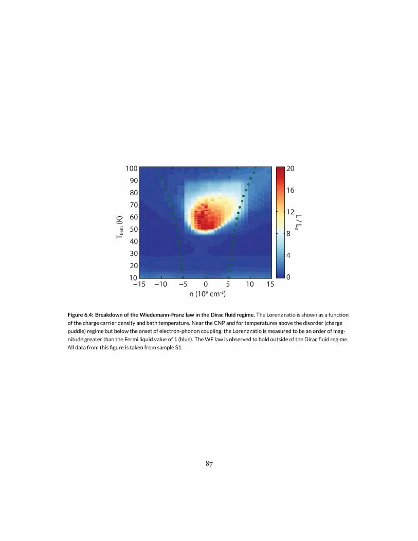
0

4

8

12

16

20

L / L

0

10

20

30

40

50

60

70

80

90

100

Tb

ath

(K

)

−10−15 15−5 0 5 10

n (109 cm-2)

Figure 6.4: Breakdown of the Wiedemann-Franz law in the Dirac fluid regime. The Lorenz ratio is shown as a functionof the charge carrier density and bath temperature. Near the CNP and for temperatures above the disorder (charge

puddle) regime but below the onset of electron-phonon coupling, the Lorenz ratio is measured to be an order of mag-

nitude greater than the Fermi liquid value of 1 (blue). TheWF law is observed to hold outside of the Dirac fluid regime.

All data from this figure is taken from sample S1.

87

Our observation of the breakdown of the WF law in graphene is consistent with the emergence

of the DF. Fig. 6.4 shows the full density and temperature dependence of the experimentally mea-

sured Lorenz ratio in order to highlight the presence of the DF. The blue colored region denotes

L ∼ L0, suggesting the carriers in graphene exhibit FL behavior. The WF law is violated in the DF

(yellow-red) with a peak Lorenz ratio 22 times larger thanL0. The green dotted line shows the cor-

responding nmin(T ) for this sample; the DF is found within this regime, indicating the coexistence

of thermally populated electrons and holes. We find that disorder and phonon scattering bound the

temperature range of the Dirac fluid, Tdis < T < Tel−ph.

We investigate the effect of impurities on hydrodynamic transport by comparing the results ob-

tained from samples with varying disorder. Fig. 6.5a shows nmin as a function of temperature for

three samples used in this study. nmin(T = 0) is estimated as 5, 8, and 10×109 cm−2 in samples S1,

S2, and S3, respectively. All devices show qualitatively similar Dirac fluid behavior; the largest value

ofL/L0 measured in the Dirac fluid regime is 22, 12 and 3 in samples S1, S2, and S3, respectively

(Fig. 6.5b). For a direct comparison, we showL(n) for all three samples at the same temperature

(60K) in Fig. 6.5c. We find that cleaner samples not only have a more pronounced peak but also a

narrower density dependence, as predicted [74, 61].

More quantitative analysis ofL(n) in our experiment can be done by employing a quasi-relativistic

hydrodynamic theory of the DF incorporating the effects of weak impurity scattering [87, 74, 61]

L =LDF

(1 + (n/n0)2)2 (6.2)

88

0 100 2000

5

10

15

20

25

Temperature (K)L

/ L

0

B

1 10 100 1000109

1010

1011

Temperature (K)

nm

in (

cm-2

)

DisorderLimited

ThermallyLimited

S3S2S1

A

−6 −4 −2 0 2 4 60

4

8

12

16

20

n (1010 cm−2)

L/L

0

C

40 60 80 1000

2

4

6

8

10

T (K)

H

(eV

/µm

2)

CHe

h

-V+Ve

h

∆Vg = 0

Figure 6.5: Disorder in the Dirac fluid. (A)Minimum carrier density as a function of temperature for all three samples.

At low temperature each sample is limited by disorder. At high temperature all samples become limited by thermal

excitations. Dashed lines are a guide to the eye. (B) The Lorenz ratio of all three samples as a function of bath temper-

ature. The largestWF violation is seen in the cleanest sample. (C) The gate dependence of the Lorenz ratio is well fitto hydrodynamic theory of Ref. [74, 61]. Fits of all three samples are shown at 60K . All samples return to the Fermi

liquid value (black dashed line) at high density. Inset shows the fitted enthalpy density as a function of temperature

and the theoretical value in clean graphene (black dashed line). Schematic inset illustrates the difference between heat

and charge current in the neutral Dirac plasma.

89

where

LDF =HvFlmT 2σmin

and n20 =

Hσmin

e2vFlm. (6.3)

Here vF is the Fermi velocity in graphene, σmin is the electrical conductivity at the CNP,H is the

fluid enthalpy density, and lm is the momentum relaxation length from impurities. Two parame-

ters in Eqn. 6.2 are undetermined for any given sample: lm andH. For simplicity, we assume we

are well within the DF limit where lm andH are approximately independent of n. We fit the exper-

imentally measuredL(n) to Eqn. 6.2 for all temperatures and densities in the Dirac fluid regime

to obtain lm andH for each sample. Fig. 6.5C shows three representative fits to Eqn. 6.2 taken at

60K . lm is estimated to be 1.5, 0.6, and 0.034 µm for samples S1, S2, and S3, respectively. For the

system to be well described by hydrodynamics, lm should be long compared to the electron-electron

scattering length of∼ 0.1 µm expected for the Dirac fluid at 60K [73]. This is consistent with

the pronounced signatures of hydrodynamics in S1 and S2, but not in S3, where only a glimpse of

the DF appears in this more disordered sample. Our analysis also allows us to estimate the ther-

modynamic quantityH(T ) for the DF. The Fig. 6.5c inset shows the fitted enthalpy density as a

function of temperature compared to that expected in clean graphene (dashed line) [73], excluding

renormalization of the Fermi velocity. In the cleanest sampleH varies from 1.1 − 2.3eV/µm2 for

Tdis < T < Tel−ph. This enthalpy density corresponds to∼ 20meV or∼ 4kBT per charge carrier

— about a factor of 2 larger than the model calculation without disorder [73].

To fully incorporate the effects of disorder, a hydrodynamic theory treating inhomogeneity non-

perturbatively is necessary [88, 89]. The enthalpy densities reported here are larger than the the-

90

oretical estimation obtained for disorder free graphene, consistent with the picture that chemical

potential fluctuations prevent the sample from reaching the Dirac point. While we find thermal

conductivity well described by Ref. [74, 61], electrical conductivity increases slower than expected

away from the CNP, a result consistent with hydrodynamic transport in a viscous fluid with charge

puddles [89].

In a hydrodynamic system, the ratio of shear viscosity η to entropy density s is an indicator of the

strength of the interactions between constituent particles. It is suggested that the DF can behave as a

nearly perfect fluid [73]: η/s approaches a conjecture by Kovtun-Son-Starinets: (η/s)/(ℏ/kB) ≳

1/4π for a strongly interacting system [90]. A non-perturbative hydrodynamic framework can be

employed to estimate η, as we discuss elsewhere [89]. A direct measurement of η is of great interest.

We have experimentally discovered the breakdown of the WF law and provided evidence for the

hydrodynamic behavior of the Dirac fermions in graphene. This provides an experimentally realiz-

able Dirac fluid and opens the way for future studies of strongly interacting relativistic many-body

systems. Beyond a diverging thermal conductivity and an ultra-low viscosity, other peculiar phe-

nomena are expected to arise in this plasma. The massless nature of the Dirac fermions is expected

to result in a large kinematic viscosity, despite a small shear viscosity η. Observable hydrodynamic

effects have also been predicted to extend into the FL regime [91]. The study of magnetotransport

in the DF will lead to further tests of hydrodynamics [74, 87].

91

6.3 Sample Fabrication

Single layer graphene is encapsulated in hexagonal boron nitride on an n-doped silicon

wafer with 285 nm SiO2 [50] and is subsequently annealed in vacuum for 15minutes at 350 C .

It is then etched using reactive-ion-etching (RIE) to define the width of the device. A second etch

mask is then lithographically defined to overlap with the sample edge, leaving the rest of the sample

rectangular shaped with the desired aspect ratio. After the RIE is performed, the same etch mask is

used as the metal deposition mask, upon which Cr/Pd/Au (1.5 nm / 5 nm / 200 nm) is deposited.

The resulting Ohmic contacts show low contact resistances and small PN junction effects due to

their minimum overlap with device edge.

6.4 Optimizing samples for high frequency thermal conductiv-

ity measurements

To measure the electronic thermal conductivity κe of graphene using high frequency

Johnson noise the sample design should be made with three additional considerations: stray chip

capacitance, resistance of the lead wires, and sample dimensions that enhance electron diffusion

cooling over phonon coupling.

Johnson noise thermometry (JNT) relies on measuring the total noise power emitted in a speci-

92

fied frequency band and relating that to the electronic temperature on the device; to maximize the

sensitivity, high frequency and wide bandwidth measurements should be made [10]. In the tem-

perature range discussed here, the upper frequency limit for JNT is typically set by the amount of

stray capacitance from the graphene, lead wires, and contact pads to the Si back gate. This is mini-

mized by using short, narrow lead wires and small (50 µm × 50 µm) bonding pads resulting in an

estimated 4 pF stray capacitance.

The amount of Johnson noise emitted between any two terminals is proportional to the mean

electronic temperature between them where each point in space is weighted by its local resistance.

Therefore, to maximize the signal coming from the graphene, contact resistance should be kept at

a minimum. To compensate for the narrow lead wires, we deposit a thicker layer (200 nm) of gold

resulting in an estimated total contact resistance of< 80Ω.

Lastly, to effectively extract κe from the total electronic thermal conductanceGth we want to en-

hance the electron diffusion cooling pathway with respect to the electron-phonon cooling pathway

(see section 4.1 for details). This can be accomplished by keeping the length of the sample short as

the total power coupled into the lattice scales as the area of the device while diffusion cooling scales

as 1/R. In addition, the device should be made wide to minimize the effects of disordered edges. We

find these high aspect ratio samples (∼ 3 : 1) are ideal for our measurements and serve the addi-

tional purpose of lowering the total sample resistance allowing us to impedance match over a wider

bandwidth.

93

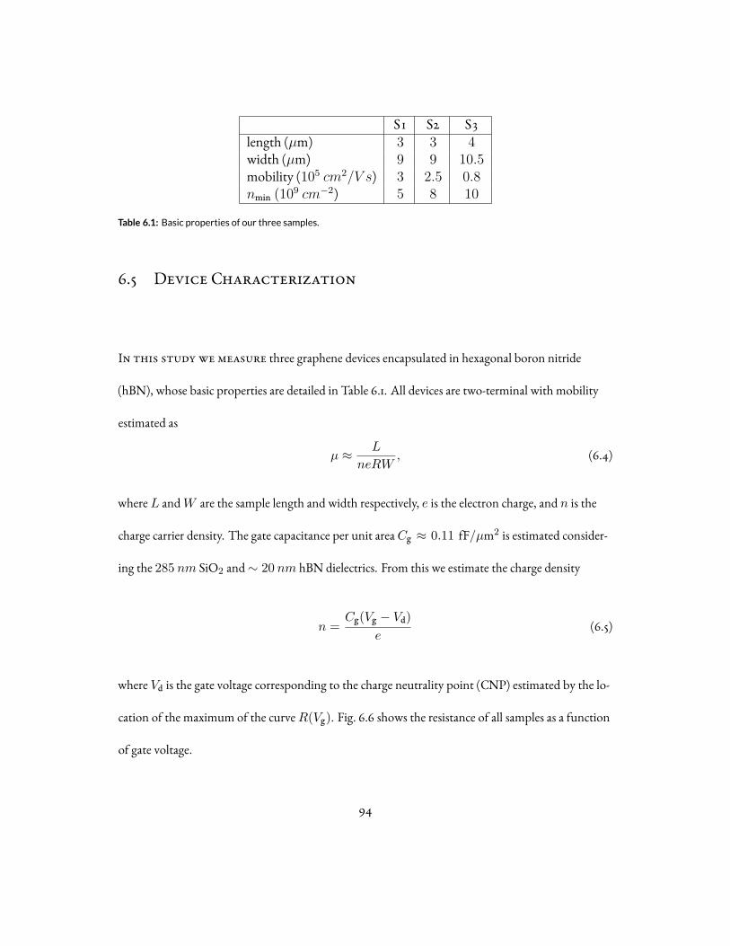
S1 S2 S3length (µm) 3 3 4width (µm) 9 9 10.5mobility (105 cm2/V s) 3 2.5 0.8nmin (10

9 cm−2) 5 8 10

Table 6.1: Basic properties of our three samples.

6.5 Device Characterization

In this study we measure three graphene devices encapsulated in hexagonal boron nitride

(hBN), whose basic properties are detailed in Table 6.1. All devices are two-terminal with mobility

estimated as

µ ≈ L

neRW, (6.4)

whereL andW are the sample length and width respectively, e is the electron charge, and n is the

charge carrier density. The gate capacitance per unit areaCg ≈ 0.11 fF/µm2 is estimated consider-

ing the 285 nm SiO2 and∼ 20 nm hBN dielectrics. From this we estimate the charge density

n =Cg(Vg − Vd)

e(6.5)

where Vd is the gate voltage corresponding to the charge neutrality point (CNP) estimated by the lo-

cation of the maximum of the curveR(Vg). Fig. 6.6 shows the resistance of all samples as a function

of gate voltage.

94

−5 −4 −3 −2 −1 0 1 2 3 4 50

1

2

3

Vg (V)

R (

KΩ

)

S1

S2

S3

Figure 6.6: 2-terminal resistanceR vs. back gate voltage for the 3 samples used in this report.

6.6 Bipolar Diffusion

The bipolar diffusion effect occurs when different charge carriers of opposite sign move in

the same direction under an applied temperature gradient. The thermal conductivity κ, in the ab-

sence of net electric current flow, is given in Ref. [92]:

κ ≡(κe −

Tα2e

σe

)+

(κh −

Tα2h

σh

)+

Tσeσh

σe + σh

(αe

σe− αh

σh

)2

(6.6)

The first two terms in the above equations are the thermal conductivity of electrons and holes re-

spectively. The third term is the bipolar diffusion term, and accounts for the possibility of electrons

and holes flowing in the same direction.

Bipolar diffusion has been used to explain the thermal conductivity of narrow gap semiconduc-

tors, such as bismuth telluride, when the chemical potential is close to the midgap. Estimates of the

95

Lorenz ratio in bismuth telluride have been reported as high as 7.2L0 in Ref. [93]. In graphene, the

two types of charge carriers correspond to above/below the Dirac point. To use the formula (6.6) re-

quires the assumption that interactions between electrons and holes are negligible. If this is the case,

it is reasonable to employ kinetic theory to estimate σe,h, αe,h and κe,h. This was shown in Ref. [94]

and we state the formalism here for completeness.

Employing the ultrarelativistic band structure of graphene near the CNP, the transport coeffi-

cients are given by:

σe =

∫d2k2π2

τe(k)v2FF(ℏvFk ± µ

kBT

), (6.7a)

αe = ±∫

d2k2π2

τe(k)(ℏvFk ± µ)v2FF(ℏvFk ± µ

kBT

), (6.7b)

κe =

∫d2k2π2

τe(k)(ℏvFk ± µ)2v2FF(ℏvFk ± µ

kBT

), (6.7c)

where τe,h are suitably defined energy relaxation times for electrons and holes, we use a± sign for

electrons/holes, and

F(x) ≡ 1

kBT

ex

(1 + ex)2. (6.8)

Given a choice of τ , it is straightforward to numerically integrate these equations. This was done

in Ref. [94] for some choices of τ ; we have checked additional choices. We compare the result of

this two-band formalism at the CNP, to the same data for S1 used in Fig. 6.5. We can rule out the

canonical bipolar diffusion (BD) explanation of our data for the following reasons:

1. The BD theory predicts thatL/LWF is independent of temperature at the CNP in a cleansample. Adding disorder only adds a very weak temperature dependence [94]. This is in

96

Temperature [K]0

5

10

15

20

25

1 100

S1Yoshino-Murata ∆ε = 0 meV

Yoshino-Murata ∆ε = 50 meV

L / L

0

clean graphene BD

disordered graphene BD

Figure 6.7: Comparison of the Lorenz ratio in graphene between bipolar diffusion theory [94] and our experimental

data. The sharp temperature dependence ofL is inconsistent with bipolar diffusion (see green dashed lines). This

sharp behavior is predicted in hydrodynamics [89].

stark contrast to our data – see Figure 6.7. Hydrodynamic models do predict a sharp temper-ature dependence inL [89].

2. Simple models of BD in the presence of charge puddles with local chemical potential fluc-tuations of 50 meV or higher predict factor of 2 violations of the WF law [94], and a weakdependence ofL on disorder, compared to hydrodynamics. In contrast we see a sharp de-pendence on disorder, comparing our three samples (Figure6.5). In samples where chemicalpotential fluctuations are comparable to 50meV , the WF law is obeyed to within 40% [51].

3. Working under the theory of [95], τ(k) ∼ |k|, and hence the maximal Lorenz ratioL/LWF ≈4 [94] – well below to our experimental observation ofL/LWF ≈ 22.

4. The BD theory of [94] predictsL/LWF ≳ 0.8 under all conditions. Hydrodynamics pre-dicts that this ratio can become arbitrarily small in a clean sample, and we have indeed ob-servedL/LWF ∼ 1/3 at finite density in the DF in sample S1, only consistent with hydrody-namics.

97

Turn a switch and the light goes on. The layman’s per-

ception is that this is like opening a tap so that the water

starts running. But this analogy is misleading.

Jan Zaanen

7Hydrodynamic framework

In exotic materials, as electron-electron interactions begin to dominate over electron-impurity

and electron-phonon scattering, new theoretical tools are needed to effectively model heat and

charge transport. One such method, described in detail below, is to abandon the idea of quasipar-

ticles altogether and instead rely on tracking macroscopically conserved quantities such as energy,

98

Figure 7.1: Dis nguishing different flow regimes. (Le ) In conventional metals, the flow of electrical current is due

to electrons (balls) moving independently as a consequence of quantum physics while scattering against crystal im-

perfections (bumpers). (Right) In normal fluids such as water, themolecules collide with each other, equilibrating in a

macroscopic fluid that is described by the theory of hydrodynamics. Electrons in particular solids that form strongly in-

teracting quantum systems are also found to exhibit hydrodynamic transport properties (ref. [55, 96, 97]). Taken from

ref. [98], reprinted with permission fromAAAS license number 4082140628269

momentum, and charge (hydrodynamics). The difficulty with this technique is the inclusion of mo-

mentum relaxing scattering events, such as those due to impurities. It is possible to include these

effects to first order by modeling the hydrodynamic equations in the presence of a non-uniform

(but slowly varying) potential similar that shown [53] to exist in graphene. While this method has

been applied with much success to describe the Dirac fluid, it is worth noting that, for the devices

described in chapter 6, the electron-electron scattering rate is of the same order as other relevant

scatting rates in the system; as such, a Boltzmann approach with the inclusion of an inter-particle

scattering time is feasible [54] (Fig. 7.2 illustrates the regimes applicable to the two frameworks).

Below we present the original text of [89]. Reprinted with permission from A. Lucas, J. Crossno,

K. C. Fong, P. Kim and S. Sachdev, “Hydrodynamic transport in quantum critical fluids and in the

Dirac fluid in graphene”, Physical Review B93 075426 (2016). Copyright (2016) by the American

Physical Society

99

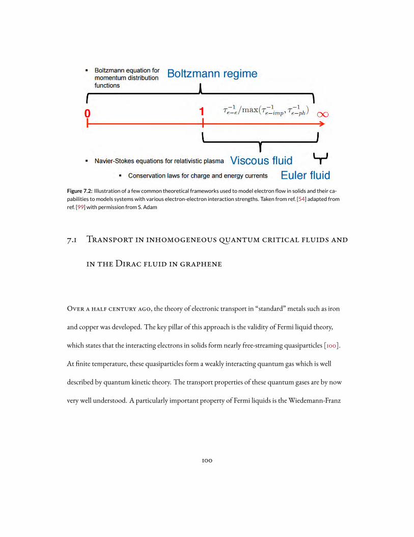
Figure 7.2: Illustration of a few common theoretical frameworks used tomodel electron flow in solids and their ca-

pabilities tomodels systemswith various electron-electron interaction strengths. Taken from ref. [54] adapted from

ref. [99] with permission from S. Adam

7.1 Transport in inhomogeneous quantum critical fluids and

in the Dirac fluid in graphene

Over a half century ago, the theory of electronic transport in “standard” metals such as iron

and copper was developed. The key pillar of this approach is the validity of Fermi liquid theory,

which states that the interacting electrons in solids form nearly free-streaming quasiparticles [100].

At finite temperature, these quasiparticles form a weakly interacting quantum gas which is well

described by quantum kinetic theory. The transport properties of these quantum gases are by now

very well understood. A particularly important property of Fermi liquids is the Wiedemann-Franz

100

law, which states that†

L ≡ κ

σT=

π2

3

k2Be2

≡ LWF. (7.1)

Here κ is the electronic contribution to thermal conductivity, σ is the electrical conductivity, T is

the temperature, andL is the Lorenz ratio. Implicit in the above equation is that the dominant

interactions are between impurities or phonons and quasiparticles, and in most metals this is true:

the interaction time between quasiparticles is typically 104 times longer than the interaction times

between quasiparticles and impurities or phonons [20].

Also over a half century ago, a study of the consequences of hydrodynamic behavior on correla-

tion functions and transport in interacting quantum systems was initiated [56]. Hydrodynamics

is a framework for understanding the collective motion of the quasiparticles in a solid, or any other

interacting quantum or classical system, so long as the microscopic degrees of freedom reach thermal

equilibrium locally. In a solid, this interaction time must be the fastest time scale in the problem to

see hydrodynamic behavior, but since quasiparticles in a Fermi liquid interact with each other only

very weakly, observing hydrodynamics in electron fluids is notoriously hard. Even in the purest met-

als where hydrodynamic behavior can be observed, such as in GaAs [57, 101, 102], the resulting fluid

is often a Fermi liquid. The resulting dynamics is the fluid dynamics of (quantum) gases. More re-

cent theoretical work on hydrodynamics in Fermi liquids includes [103, 104, 105, 106, 107, 108], and

recent experimental work includes [96, 97].

Fermi liquid theory is known to fail in a variety of experimentally realized metals in two or more

†Below we have assumed that the charge of the quasiparticles is±e, with e the charge of the electron –this is essentially always the case.

101

spatial dimensions – most famous among these is the strange metal phase of the cuprate supercon-

ductors [109, 110, 68] which does not have quasiparticle excitations. A slightly more theoretically

controlled and better understood example of a state of quantum matter without quasiparticles is the

quasi-relativistic Dirac fluid in the semimetal graphene. The Dirac fluid, which effectively lives in

two spatial dimensions, has also been argued to be strongly interacting at experimentally achievable

temperatures [67, 60, 79, 111] due to ineffective Coulomb screening [66]. Although it is separated

from the Fermi liquid by a crossover, and not a (thermal) phase transition, its proximity to a (sim-

ple) zero temperature quantum critical point at charge neutrality means that the phenomenology

of the Dirac fluid is expected to differ strongly from Fermi liquid theory. Due to the high spatial

dimensionality,† the development of a predictive quantitative theory of these systems is notori-

ously hard. A major theme in recent work has been quantum criticality [112, 113], which opens up

the possibility for borrowing powerful techniques from high energy physics, but even in this case

very little is known about experimentally relevant regime of finite temperature and density. One

of the only remaining techniques for understanding these systems is hydrodynamics, as many fea-

tures of hydrodynamics are universal and model independent, and the strongly interacting quantum

physics is captured entirely by the coefficients in otherwise classical differential equations. Such

fluids are quantum analogues of classical liquids such as water, which are strongly interacting (al-

beit with negligible quantum entanglement) insofar as they do not admit a controllable description

via kinetic theory. Furthermore, it has been shown [87] that strongly interacting quantum critical

†Quantum dynamics in one dimension, which is often integrable, is described using very different tech-niques and has qualitatively distinct features.

102

fluids have a somewhat different hydrodynamic description than the canonical Fermi liquids de-

scribed above, and this can lead to very different hydrodynamic properties, including in transport

[87, 60, 79, 74, 73, 61, 114], as we will review in this paper.

Using novel techniques to measure thermal transport [51, 41, 10], the Dirac fluid has finally been

observed in monolayer graphene, and evidence for its hydrodynamic behavior has emerged [55], as

we will detail. However, existing theories of hydrodynamic transport are not consistent with the

simultaneous density dependence in experimentally measured thermal and electrical conductivities.

In this paper, we improve upon the hydrodynamic theory of [87], describe carefully effects of finite

density, and develop a non-perturbative relativistic hydrodynamic theory of transport in electron

fluids near a quantum critical point. Under certain assumptions about the equations of state of the

Dirac fluid, our theory is quantitatively consistent with experimental observations. The techniques

we employ are included in the framework of [88], which developed a hydrodynamic description

of transport in relativistic fluids with long wavelength disorder in the chemical potential. [88] was

itself inspired by recent progress employing the AdS/CFT correspondence to understand quantum

critical transport in strange metals [115, 114, 116, 117, 118, 119, 120, 121, 122], but as we will discuss, this

theory is also well suited to describe the physics of graphene.

7.1.1 Summary of Results

The recent experiment [55] reported order-of-magnitude violations of the Wiedemann-Franz

law. The results were compared with the standard theory of hydrodynamic transport in quantum

103

critical systems [87], which predicts that

σ(n) = σq +e2v2Fn

2τ

H, (7.2a)

κ(n) =v2FHτ

T

σq

σ(n), (7.2b)

where e is the electron charge, s is the entropy density, n is the charge density (in units of length−2),

H is the enthalpy density, τ is a momentum relaxation time, and σq is a quantum critical effect,

whose existence is a new effect in the hydrodynamic gradient expansion of a relativistic fluid. Note

that up to σq, σ(n) is simply described by Drude physics. The Lorenz ratio then takes the general

form

L(n) = LDF

(1 + (n/n0)2)2, (7.3)

where

LDF =v2FHτ

T 2σq, (7.4a)

n20 =

Hσq

e2v2Fτ. (7.4b)

L(n) can be parametrically larger thanLWF (as τ → ∞ and n ≪ n0), and much smaller (n ≫

n0). Both of these predictions were observed in the recent experiment, and fits of the measured

L to (7.3) were quantitatively consistent, until large enough nwhere Fermi liquid behavior was

restored. However, the experiment also found that the conductivity did not grow rapidly away from

104

hole FL elec. FLDirac fluid

400 200 0 200 4000

0.5

1

1.5

2

n (µm2)

(k1

)hole FL elec. FLDirac fluid

400 200 0 200 4000

2

4

6

8

10

n (µm2)

(nW

/K)

Figure 1: testingFigure 7.3: A comparison of our hydrodynamic theory of transport with the experimental results of [55] in clean sam-

ples of graphene atT = 75K.We study the electrical and thermal conductances at various charge densitiesn near

the charge neutrality point. Experimental data is shown as circular red datamarkers, and numerical results of our the-

ory, averaged over 30 disorder realizations, are shown as the solid blue line. Our theory assumes the equations of state

described in (7.27) with the parametersC0 ≈ 11,C2 ≈ 9,C4 ≈ 200, η0 ≈ 110,σ0 ≈ 1.7, and (7.28) withu0 ≈ 0.13. The yellow shaded region showswhere Fermi liquid behavior is observed and theWiedemann-Franz law

is restored, and our hydrodynamic theory is not valid in or near this regime. We also show the predictions of (7.2) as

dashed purple lines, and have chosen the 3 parameter fit to be optimized forκ(n).

n = 0 as predicted in (7.2), despite a large peak in κ(n) near n = 0, as we show in Figure 7.3.

Furthermore, the theory of [87] does not make clear predictions for the temperature dependence of

τ , which determines κ(T ).

In this paper, we argue that there are two related reasons for the breakdown of (7.2). One is that

the dominant source of disorder in graphene – fluctuations in the local charge density, commonly

referred to as charge puddles [81, 123, 82, 53] – are not perturbatively weak, and therefore a non-

perturbative treatment of their effects is necessary.† The second is that the parameter τ , even when

it is sharply defined, is intimately related to both the viscosity and to n, and this n dependence is

neglected when performing the fit to (7.2) in Figure 7.3. We develop a non-perturbative hydrody-

namic theory of transport which relies on neither of the above assumptions, and gives us an explicit

†See [80, 124] for a theory of electrical conductivity in charge puddle dominated graphene at low tempera-tures.

105

puddle FLs phononsDirac fluid

40 50 60 70 80 900.2

0.3

0.4

0.5

T (K)

(k1

)puddle FLs phononsDirac fluid

40 50 60 70 80 900

2

4

6

8

10

T (K)

(nW

/K)

Figure 1: testingFigure 7.4: A comparison of our hydrodynamic theory of transport with the experimental results of [55] in clean sam-

ples of graphene at the charge neutrality point (n = 0). We use no new fit parameters compared to Figure 7.3. The

yellow shaded region denotes where Fermi liquid behavior is observed; the purple shaded region denotes the likely

onset of electron-phonon coupling.

formula for τ in the limit of weak disorder. The key assumption for the validity of our theory is

that the size of the charge puddles is comparable to or larger than the electron interaction length

scale, which is about 100 nm. Experimental evidence suggests this is marginally true in graphene

samples mounted on hexagonal boron nitride [53], as was done in [55]. Although we cannot ana-

lytically solve our theory non-perturbatively, we perform numerical computations of the transport

coefficients in disordered fluids, and compare the results to the experimental data in Figure 7.3. Our

simultaneous fit to κ(n) and σ(n) shows improved quantitative agreement with both sets of data

in the Dirac fluid regime. We further compare in Figure 7.4 the temperature dependence of κ and

σ between our numerics and the experiment, using no new fitting parameters, and find satisfactory

quantitative agreement in the Dirac fluid regime.

Figure 7.5 shows a cartoon of the regime of validity of our hydrodynamic theory. The fact that

the charge puddles may be substantial, while the entropy and energy densities are much more con-

stant, helps to explain why the perturbative description of transport is much better for κ than σ, as

106

x

nn(x) < 0

n(x) > 0

s(x) > 0lee

Figure 7.5: A cartoon of a nearly quantum critical fluid where our hydrodynamic description of transport is sensible.

The local chemical potentialµ(x) always obeys |µ| ≪ kBT , and so the entropy density s/kB is much larger than the

charge density |n|; both electrons and holes are everywhere excited, and the energy density ϵ does not fluctuate asmuch relative to themean. Near charge neutrality the local charge density flips sign repeatedly. The correlation length

of disorder ξ is much larger than lee, the electron-electron interaction length.

the perturbative approach works well in a nearly homogeneous fluid. In coming years the quality of

graphene samples will improve, and the charge puddle size may grow larger than 100 nm, allowing

us to observe the clean hydrodynamic limit described by (7.2). As present day samples are just clean

enough to observe hydrodynamics, our determination of the equations of state should be under-

stood as preliminary.

Although the focus of this paper is on the Dirac fluid in graphene, this is because of the experi-

mental motivation for this work. Our theory has broader validity, and we will introduce it in the

more general context of transport in a disordered electronic fluid near a quantum critical point with

manifest Lorentz invariance, with the microscopic Fermi velocity vF playing the role of the speed

of light. The Dirac fluid is not strictly Lorentz invariant, but we will justify the validity of our ap-

proach even in this system. While the Dirac fluid in graphene is currently the only experimentally

realized strongly interacting condensed matter system with evidence for electronic hydrodynam-

107

ics [55], in the future surface states in topological insulators in three spatial dimensions may host

strongly interacting electron fluids [125]. Strongly interacting three dimensional materials includ-

ing Weyl semimetals [126, 127, 128] may also give rise to novel phenomena relevant for transport

[129, 130].

7.1.2 Outline

The outline of this paper is as follows. We briefly review the definitions of transport coeffi-

cients in Section 7.2. In Section 7.3 we develop a theory of hydrodynamic transport in the elec-

tron fluid, assuming that it is Lorentz invariant. We discuss the peculiar case of the Dirac fluid in

graphene in Section 7.4, and argue that deviations from Lorentz invariance are small. We describe

the results of our numerical simulations of this theory in Section 7.5, and directly compare our sim-

ulations with recent experimental data from graphene [55]. The experimentally relevant effects of

phonons are qualitatively described in Section 7.6. We conclude the paper with a discussion of fu-

ture experimental directions. AppendixB contains technical details of our theory.

In this paper we use index notation for vectors and tensors. Latin indices ij · · · run over spa-

tial coordinates x and y; Greek indices µν · · · run over time t as well. We will denote the time-

like coordinate ofAµ asAt. Indices are raised and lowered with the Minkowski metric ηµν ≡

diag(−1, 1, 1). The Einstein summation convention is always employed.

108

7.2 Transport Coefficients

Let us begin by defining the thermoelectric response coefficients of interest in this paper. Sup-

pose that we drive our fluid by a spatially uniform, externally applied, electric fieldEi (formally, an

electrochemical potential gradient), and a temperature gradient−∂iT . We will refer to−∂jT as

Tζj , with ζj = −T−1∂jT , for technical reasons later. As is standard in linear response theory, we

decompose these perturbations into various frequencies, and focus on the response at a single fre-

quency ω. Time translation invariance implies that the (uniformly) spatially averaged charge current

⟨Ji⟩ and the spatially averaged heat current ⟨Qi⟩ are also periodic in time of frequency ω, and are

related toEi and ζi by the thermoelectric transport coefficients:

⟨Ji⟩

⟨Qi⟩

e−iωt =

σij(ω) Tαij(ω)

T αij(ω) T κij(ω)

Ej

ζj

e−iωt. (7.5)

In a typical disordered system, we expect that σij , αij , αij and κij are all proportional to δij . In

our numerics, finite size effects introduce some anisotropy; our theory is valid in this more general

scenario.

In fact, (7.5) is somewhat subtle. Implicit in the definitions of the transport coefficients are a set

of boundary conditions. In the definitions in (7.5), we have assumed that we tuneEi and ζi, and

then measure Ji andQi. However, usually in experiments one fixes Ji, as electronic measurements

are far easier to control. One then can fix eitherEi or ζi. So while it is straightforward to measure

109

σij by setting ζi = 0, one measures not κij but instead κij , defined as

⟨Qi⟩|⟨Ji⟩=0 = Tκijζj . (7.6)

Straightforward manipulations give that σijEj = −Tαijζj , and therefore that

κij = κij − T αikσ−1kl αlj . (7.7)

These definitions are general and independent of our hydrodynamic theory.

7.3 Relativistic Hydrodynamics

We now develop a theory of relativistic hydrodynamics of the electronic plasma in a disordered

metal, where the disorder is introduced by a spatially dependent chemical potential µ0(x). So long

as the length scale ξ ∼ |µ0|/|∂xµ0| over which this function varies is much larger than the electron-

electron scattering length lee ∼ ℏvF/kBT , it is sensible to treat the fluid as locally homogeneous,

with parameters such as energy density and viscosity locally being functions of µ0 alone. This exter-

nal chemical potential acts as an external source of energy and momentum for the electronic plasma,

and can be sourced by lattice defects or impurities, either in the (semi)metal itself, or in the substrate

it is placed on, for two-dimensional materials such as graphene [81, 53]. Our theory here is analo-

gous to [88], and similar to the earlier work [103] in non-relativistic fluids. However, [88] focused

110

mostly on the mathematical consequences of relativistic hydrodynamics, particularly in regards to

holographic models. Our focus here is on practical consequences in realistic quantum critical fluids

where µ ≪ kBT , and where the equations of state are tightly constrained by scale invariance (see

Appendix B.1).

Previous theories of hydrodynamic transport assumed that disorder was parametrically weak,

and so momentum is a nearly conserved quantity [87, 60]. Such theories can be shown to be a per-

turbative limit of the more general approach that we advocate below: see [88] and Appendix B.3.

However, near the charge-neutrality point, non-perturbative effects can become important [88].

Since this is the regime where [55] observed evidence for hydrodynamic behavior, it is necessary to

treat transport in the charge-neutral fluid carefully and to study non-perturbative physics. We be-

gin with a general discussion of the equations of state of a relativistic plasma, and then outline our

non-perturbative hydrodynamic description of transport.

Though our focus in this paper is on the case of two spatial dimensions, it is straightforward to

generalize our theory to higher dimensions.

7.3.1 Hydrodynamic Equations

Let us review the structure of relativistic hydrodynamics, which was derived carefully in

[87]. Hydrodynamics is a general framework which describes the relaxation of an ergodic and locally

thermalizing (classical or quantum) system to global thermal equilibrium, or as close to global equi-

librium as boundary conditions or external sourcing allow. The assumption of local thermalization

111

implies that the only quantities with dynamics on long time scales (compared to the local thermal-

ization time lee/vF) are quantities that are globally conserved, up to external sources. In a typical the-

ory, these will be charge, energy and momentum, and we will assume this to be the case for graphene

as well. Hydrodynamics is a systematic way to truncate equations of motion for the local charge

density n(x), energy density ϵ(x) and momentum densityΠi(x), by treating the perturbative pa-

rameter as lee∂µ. In fact, it is typical to instead study the dynamics of the thermodynamic conjugate

variables: chemical potential µ(x), temperature T (x) and relativistic velocity uµ(x), respectively.

uµ is subject to the usual constraint uµuµ = −v2F .

Note that throughout this paper, “charge density” n refers to the number density of electrons,

minus the number density of holes: n = nelec − nhole. Thus, there are no factors of e in the defini-

tion of n, or chemical potential µ.†

The equations of motion of hydrodynamics are the local conservation laws, up to external sources.

We apply an external chemical potential µ0 via an external electromagnetic fieldAtext = −µ0(x)/e,

Aiext = 0. We employ relativistic notation with vF = 1 temporarily. The equations of hydrodynam-

ics are

∂µTµν = eFµν

ext Jν , (7.8a)

∂µJµ = 0, (7.8b)

where F tiext = −F it

ext = ∂iµ0 are the only non-vanishing components, Tµν represents the expecta-

†Therefore [n] = [length]−d and [µ] = [energy].

112

tion value of the local stress-energy density, and Jµ the expectation value of the local charge density.

Tµν and Jµ must be expressed in terms of µ, T and uµ in order to obtain a closed set of equations.

One can show that there is a static solution to the hydrodynamic equations with uµ = (1, 0, 0),

T = T0 = constant, and µ(x) = µ0(x) [88]. Recall that µ0(x) is slowly varying on the length scale

ξ. We will take this solution as the background state of our fluid.

Hydrodynamics is a perturbative expansion of (7.8), where the perturbative expansion parameter

is the number of derivatives of space and time. At zeroth order, the equations of state are simply

that Tµν and Jµ are given by the thermodynamic relations we derived above:

Tµν = (ϵ+ P )uµuν + Pηµν , (7.9a)

Jµ = nuµ, (7.9b)

with ϵ the energy density and P the pressure. In the fluid’s rest frame, T tt = ϵ, T ij = Pδij , and

J t = n, with all other components vanishing. At first order, [87] showed that the most general

first derivative corrections to Tµν and Jµ consistent with symmetries and the local second law of

thermodynamics are

Tµν = (ϵ+ P )uµuν + Pηµν − 2PµρPνση∂(ρuσ) − Pµν (ζ − η) ∂ρuρ, (7.10a)

Jµ = nuµ −σq

e2(ηµν + uµuν)

(∂νµ− µ

T∂νT − eFνρ,extu

ρ), (7.10b)

with η, ζ, σq > 0, andPµν = ηµν + uµuν . Here η and ζ are the shear and bulk viscosity re-

113

spectively, and σq is a “quantum critical” conductivity [87]. Note that the external electromagnetic

fields show up in the hydrodynamic gradient expansion in the charge current; this happens because

the charged fluid is sensitive only to the gradient in the total electrochemical potential [100]. We

allow for P , n, η, ζ and σq to all be position-dependent, with their position dependence related to

µext, as we will describe shortly in more detail.

It has long been appreciated [87] that σq plays a fundamental role in hydrodynamic transport

near quantum critical points. More recently [114] argued that η could play a role in transport. We

will carefully detail how η affects transport in this paper, analytically and numerically.

In our extension of this theory to graphene, we will also allow for Coulomb interactions of the

fluid to be substantial enough to enter the hydrodynamic equations. However, this should only

alter the equations of state, as well as add a further contribution to Fµν,ext [60], and we will detail

this in the subsequent section. The constraints imposed on hydrodynamics from local positivity of

entropy production [87] are unchanged in the presence of Coulomb interactions, which are entirely

accounted for via a modified Fµνext .

It is sufficient in our calculation of σ, α and κ to simplify Tµν and Jµ and retain only the terms

linear in velocity. One finds, in d = 2:

T ti = (ϵ+ P )vi, (7.11a)

T ij = Pδij − η(∂ivj + ∂jvi

)− (ζ − η)δij∂kv

k, (7.11b)

J i = nvi −σq

e2

(∂i(µ− µ0)−

µ

T∂iT

). (7.11c)

114

We stress the novel role of σq, a new dissipative transport coefficient in a relativistic fluid, without

a direct analogue in the canonical non-relativistic fluid. This term is related to the underlying ther-

mally excited electron-hole plasma, and the fact that electrons and holes can move in opposite direc-

tions under an applied electric field, contributing a net electric current.† There is no microscopic

thermal conductivity – instead, all microscopic dissipation related to electric and thermal gradients is

controlled by σq.

7.3.2 Hydrodynamic Theory of Transport

We are now ready to detail our hydrodynamic calculation of the transport coefficients defined

in Section 7.2. We place our fluid in a box of lengthL in each direction, with periodic boundary

conditions on the fluid in every direction. We then apply a constant backgroundEi and ζi.‡ The

static solution above is no longer a solution to the hydrodynamic equations of motion, sourced by

these gradients. Now, we generically expect to excite both a spatial electric current J i, and a spatial

heat current

Qi ≡ T ti − µJ i. (7.12)

†It is qualitatively similar to the bipolar diffusion effect [92, 94] – however, in hydrodynamics the quasi-particle lifetimes are limited by ℏ/kBT , whereas in the bipolar diffusion effect these lifetimes are parametri-cally long, as in a Fermi liquid.

‡The application of a constant ζj on a periodic space is the reason why we cannot talk about driving thesystem with a constant temperature gradient, since the temperature is a periodic function in space. One canformally implement ζi through deformations of the spacetime metric and external gauge fields [131].

115

We can expand out J i andQi locally as a Taylor series inEi and ζi. The transport coefficients in

Section 7.2 are defined by retaining only the linear terms inEi and ζi, and spatially averaging over

the local charge and heat currents. It is sufficient to perform a linear response calculation about our

previously identified static solution:

µ ≈ µ0(x) + δµ(x)e−iωt, (7.13a)

T ≈ T0 + δT (x)e−iωt, (7.13b)

ut ≈ 1, (7.13c)

ui ≈ δvi(x)e−iωt, (7.13d)

and then solve the linearized hydrodynamic equations – this is equivalent to only keeping terms

linear inEi and ζi in the full solution. For ease of notation, we drop the “δ” in front of the linear

response perturbations in the remainder of the paper, but one should keep in mind that µ(x), T (x),

and vi are henceforth perturbatively small quantities.

Following [88], the linearized hydrodynamic equations (7.8) can be shown to take the following

116

form:†

−e−2∂iσq∂i e−2T−1

0 ∂iµ0σq∂i ∂jn

e−2∂iµ0σq∂i −e−2T−10 ∂iµ

20σq∂i T0∂js

n∂i s∂i −∂i(ζ − η)∂j − ∂iη∂j − ∂jη∂i

µ

T

vj

=

−e−1∂iσq(Ei − µ0ζi/e)

e−1∂iσqµ0(Ei − µ0ζi/e)

enEi + T0sζi

(7.14)

Here

s =ϵ+ P − µ0n

T0(7.15)

is the entropy density of the background fluid. s and n are not independent, and are related by ther-

modynamic Maxwell relations: see Appendix B.1. We have also employed

∂iP = n∂iµ+ s∂iT. (7.16)

In particular, s and n are position dependent functions whose position dependence is entirely de-

termined by the local chemical potential: s(x) = s(T0, µ0(x)), and similarly for n, η, and all other

coefficients in the hydrodynamic equations. The proper boundary conditions to impose on µ, T

and vj are periodicity. This forms a well-posed elliptic partial differential equation and can be nu-

merically solved: see Appendix B.5. Combining (7.11) and (7.12), along with µ, T and vi as found

†In this equation, derivatives act on all fields to the right, so ∂xη∂xvx should be read as ∂x(η∂xvx).

117

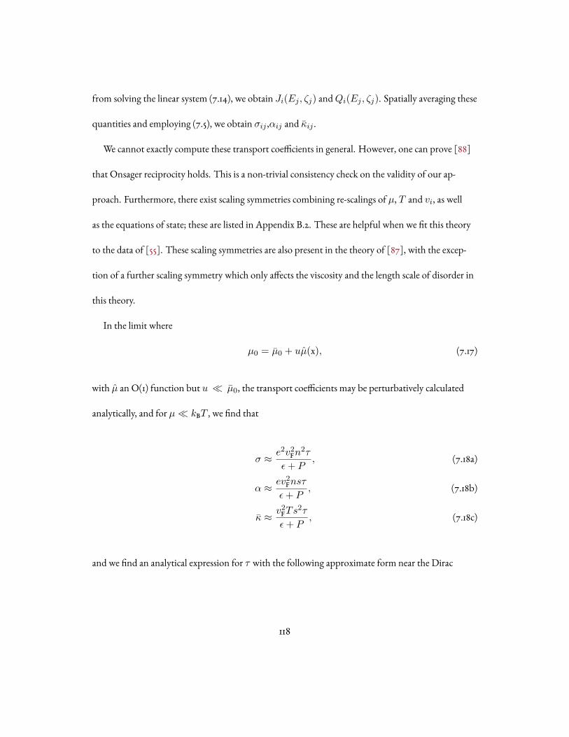
from solving the linear system (7.14), we obtain Ji(Ej , ζj) andQi(Ej , ζj). Spatially averaging these

quantities and employing (7.5), we obtain σij ,αij and κij .

We cannot exactly compute these transport coefficients in general. However, one can prove [88]

that Onsager reciprocity holds. This is a non-trivial consistency check on the validity of our ap-

proach. Furthermore, there exist scaling symmetries combining re-scalings of µ, T and vi, as well

as the equations of state; these are listed in Appendix B.2. These are helpful when we fit this theory

to the data of [55]. These scaling symmetries are also present in the theory of [87], with the excep-

tion of a further scaling symmetry which only affects the viscosity and the length scale of disorder in

this theory.

In the limit where

µ0 = µ0 + uµ(x), (7.17)

with µ an O(1) function but u ≪ µ0, the transport coefficients may be perturbatively calculated

analytically, and for µ ≪ kBT , we find that

σ ≈ e2v2Fn2τ

ϵ+ P, (7.18a)

α ≈ ev2Fnsτ

ϵ+ P, (7.18b)

κ ≈ v2FTs2τ

ϵ+ P, (7.18c)

and we find an analytical expression for τ with the following approximate form near the Dirac

118

point:

1

τ≈ v2Fu

2

2

(∂n

∂µ

)2 [ e2

σq(ϵ+ P )+

η + ζ

ξ24µ2

(ϵ+ P )3

]. (7.19)

Details of this calculation and a more precise (and complicated) formula are given in Appendix B.3.

The requirement that we are “far” from the Dirac point is that σq ≪ e2v2Fn2τ/(ϵ+P ). Everything

in (7.19) except for u is evaluated in the clean fluid with u → 0. (7.19) makes clear that if η/ξ2 is

large, the n and µ dependence of τ is not negligible even when µ ≪ kBT , and we will verify this

in numerical simulations in Section 7.5. The validity of (7.2) for κ is not guaranteed far from the

Dirac point in this perturbative limit, but can often be quite good in practice, when the density

dependence of all parameters is accounted for. Combining (7.18) and (7.19), we obtain the relativistic

analogue of the perturbative results of [103].

Noting that n ∼ µ as µ → 0, careful study of (7.2) shows that the Lorentzian form of κ(n) is

not altered by plugging in this hydrodynamic formula for τ , while the form of σ(n) can be quite

distinct, with σ(n) no longer growing quadratically at larger n. This helps explain why in Figure 7.3,

(7.2) gave a quantitatively good fit to κ(n), but not to σ(n).

7.4 The Dirac Fluid in Graphene

The previous section developed a general theory for relativistic fluids. It is often said that the

Dirac fluid in graphene is a “quantum critical” system in two spatial dimensions [132, 67, 73], and ex-

hibits behavior analogous to the quantum critical regime at finite temperatures above the superfluid-

119

insulator transition, although technical differences arise. Let us review elementary features of the

quantum critical behavior of graphene, and argue that our formalism remains appropriate for trans-

port computations.

Assuming that the electrons in graphene are non-interacting, standard band theory calculations

on a honeycomb lattice in two spatial dimensions with nearest-neighbor hopping give two species of

Dirac fermions with low-energy dispersion relation

ϵ(q) ≈ ℏvF|q|, (7.20)

Convincing experimental evidence for these massless Dirac fermions was given in [64, 65]. There is a

quantum critical point between electron and hole Fermi liquids at zero temperature in graphene, as

the chemical potential µ is tuned through the Dirac point, µ = 0. At (any experimentally accessible)

finite temperature T , and at µ ≪ T , an effectively relativistic plasma of electrons and holes forms,

interacting via a 1/r Coulomb potential. The strength of these Coulomb interactions is captured by

a dimensionless number α0 analogous to the fine structure constant:

α0 =e2

4πϵ0ϵrℏvF≈ 1

137

c

ϵrvF, (7.21)

where ϵr ∼ 4 is a dielectric constant, c ≈ 3×108 m/s is the speed of light, vF ≈ 1.1×106 m/s is the

Fermi velocity in graphene and e is the charge of the electron. In experiments, α0 ∼ O(1), and so

unlike quantum electrodynamics (αQED ≈ 1/137), interactions are strong. vF plays the role of the

120

speed of light in an effectively relativistic electron-hole plasma, and in an experimentally accessible

regime which we describe below, one can use relativistic hydrodynamics to model thermoelectric

transport in graphene.

The exception to the emergent Lorentz invariance is the photon-mediated Coulomb interactions,

which are the standard 1/r interaction of three spatial dimensions. Further, because vF ∼ c/300,

the Coulomb interaction is essentially non-local and instantaneous in time. Despite this, graphene

shares many features with a truly relativistic plasma with “speed of light” vF, including a “quantum

critical” diffusive conductivity σq [74].

Analogously to in quantum electrodynamics, α is a marginally irrelevant interaction, and so the

effective coupling constant runs. At temperature T → 0, we should replace α0 with [67]

αeff = α0

(1 +

α0

4log

Λ

T0

)−1

(7.22)

whereΛ ∼ 8.4× 104 K is a cutoff related to the graphene band structure (the energy scale at which

the dispersion is no longer linear). Note that although the running of αeff causes a logarithmically

increasing velocity vF in (7.20), when we write vF in this paper, we are always referring to the bare

velocity, 1.1× 106 m/s.

At the experimentally accessible temperatures (T0 ∼ 70K) where the plasma described above is

most likely not suppressed by local disorder in µ [55], (7.22) gives αeff ∼ 0.25. And so the experi-

ments likely probe the dynamics of a strongly interacting quasi-relativistic plasma. It is such a regime

where hydrodynamics is a good approximation. More carefully, the electron-electron scattering

121

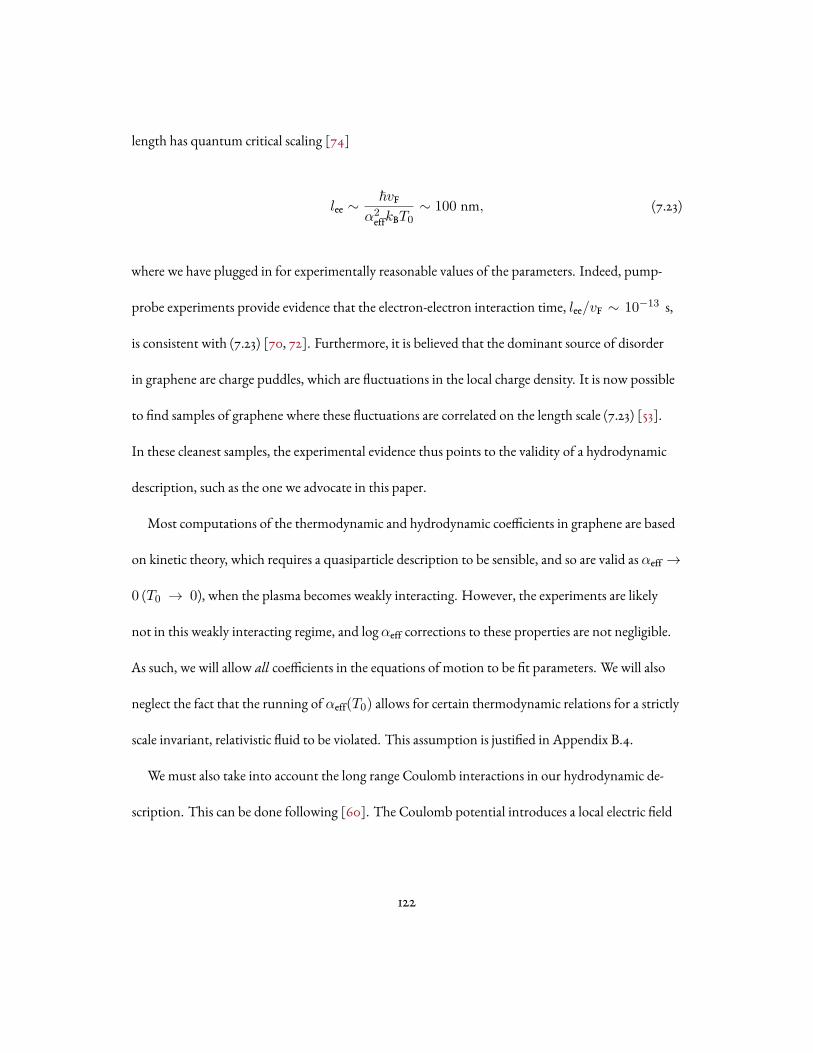
length has quantum critical scaling [74]

lee ∼ℏvF

α2effkBT0

∼ 100 nm, (7.23)

where we have plugged in for experimentally reasonable values of the parameters. Indeed, pump-

probe experiments provide evidence that the electron-electron interaction time, lee/vF ∼ 10−13 s,

is consistent with (7.23) [70, 72]. Furthermore, it is believed that the dominant source of disorder

in graphene are charge puddles, which are fluctuations in the local charge density. It is now possible

to find samples of graphene where these fluctuations are correlated on the length scale (7.23) [53].

In these cleanest samples, the experimental evidence thus points to the validity of a hydrodynamic

description, such as the one we advocate in this paper.

Most computations of the thermodynamic and hydrodynamic coefficients in graphene are based

on kinetic theory, which requires a quasiparticle description to be sensible, and so are valid as αeff →

0 (T0 → 0), when the plasma becomes weakly interacting. However, the experiments are likely

not in this weakly interacting regime, and logαeff corrections to these properties are not negligible.

As such, we will allow all coefficients in the equations of motion to be fit parameters. We will also

neglect the fact that the running of αeff(T0) allows for certain thermodynamic relations for a strictly

scale invariant, relativistic fluid to be violated. This assumption is justified in Appendix B.4.

We must also take into account the long range Coulomb interactions in our hydrodynamic de-

scription. This can be done following [60]. The Coulomb potential introduces a local electric field

122

and must be included in Fµνext :

Atext = µext − φ = µext − φext − δφ (7.24)

where

φ(x) =∫

d2y K(x − y) n(y), (7.25)

withK a Coulomb kernel whose specific form [95] is not necessary for our purposes, and the n the

charge density. At T0 = 0,K(r) = αeff/r; at finite T0, this is cut-off at long wavelengths due

to thermal screening [95]. In (7.24) we have separated the effects of Coulomb screening into two

contributions: φext, which alters the background disorder profile, so that µ0 = µext, and δφ, which

is the infinitesimal Coulomb potential created by the change in charge density δn, proportional to

Ei and ζi.

The time-independent equations of motion depend only on T , vi, the sourcesEi and ζi, and the

electrochemical potential

δΦ ≡ δµ+ δφ. (7.26)

This is a direct consequence of the tightly constrained way that Fext and µ enter the hydrodynamic

gradient expansion. If we solve for δΦ instead of δµ, we find that Coulomb screening does not affect

dc transport at all: more precisely, the equations of motion are identical to those in Section 7.3, but

with δΦ replacing δµ. That dc transport is insensitive to Coulomb screening of the hydrodynamic

degrees of freedom was also noted in [60] in a homogeneous fluid by appealing to the random phase

123

approximation.† It is therefore appropriate to directly apply the formalism of Section 7.3 to study dc

thermal and electric transport in the Dirac fluid in graphene. To maintain notation with Section 7.3,

we will continue to refer to Φ as µ in our linear response theory, with the understanding that this

includes corrections due to Coulomb screening.

7.5 Numerical Results

Having argued that the theory of Section 7.3 is an acceptable approximation for dc trans-

port in the Dirac fluid in graphene, we now present the results of numerical simulations of (7.14). In

our numerics, we assume that the equations of state of the graphene fluid are as follows:

n(µ0) =

(kBT0

ℏvF

)2[C2

µ0

kBT0+ C4

(µ0

kBT0

)3], (7.27a)

s(µ0) =k3BT

20

(ℏvF)2

[C0 +

C2

2

(µ0

kBT0

)2

− C4

4

(µ0

kBT0

)4], (7.27b)

η(µ0) =(kBT0)

2

ℏv2Fη0, (7.27c)

ζ(µ0) = 0, (7.27d)

σ(µ0) =e2

ℏσ0, (7.27e)

withC0,2,4, σ0 and η0 dimensionless constants. The form of n and s are consistent with thermody-

namic Maxwell relations – see Appendix B.1. We take the disorder profile to be random sums of sine

†See also the discussion in [100, 133].

124

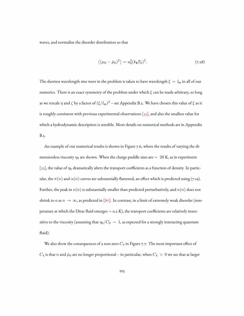
waves, and normalize the disorder distribution so that

⟨(µ0 − µ0)

2⟩= u20(kBT0)

2. (7.28)

The shortest wavelength sine wave in the problem is taken to have wavelength ξ = lee in all of our

numerics. There is an exact symmetry of the problem under which ξ can be made arbitrary, so long

as we rescale η and ζ by a factor of (ξ/lee)2 – see Appendix B.2. We have chosen this value of ξ as it

is roughly consistent with previous experimental observations [53], and also the smallest value for

which a hydrodynamic description is sensible. More details on numerical methods are in Appendix

B.5.

An example of our numerical results is shown in Figure 7.6, where the results of varying the di-

mensionless viscosity η0 are shown. When the charge puddle sizes are∼ 20K, as in experiment

[53], the value of η0 dramatically alters the transport coefficients as a function of density. In partic-

ular, the σ(n) and α(n) curves are substantially flattened, an effect which is predicted using (7.19).

Further, the peak in κ(n) is substantially smaller than predicted perturbatively, and κ(n) does not

shrink to 0 as n → ∞, as predicted in [87]. In contrast, in a limit of extremely weak disorder (tem-

perature at which the Dirac fluid emerges∼ 0.2 K), the transport coefficients are relatively insen-

sitive to the viscosity (assuming that η0/C0 ∼ 1, as expected for a strongly interacting quantum

fluid).

We also show the consequences of a non-zeroC4 in Figure 7.7. The most important effect of

C4 is that n and µ0 are no longer proportional – in particular, whenC4 > 0we see that at larger

125

6 4 2 0 2 4 60

1

2

3

4

u0 = 0.2

µ0 (meV)

(k1)

6 4 2 0 2 4 60

2

4

6

µ0 (meV)

(nW

/K)

6 4 2 0 2 4 6

500

0

500

µ0 (meV)

↵(nW

/V)

0 = 0.10 = 0.50 = 3

0.1 0.05 0 0.05 0.10

5

10

15

20

u0 = 0.002

µ0 (meV)

(k1)

0.1 0.05 0 0.05 0.10

20

40

60

µ0 (meV)

(µW

/K)

0.1 0.05 0 0.05 0.1

100

0

100

µ0 (meV)

↵(µW

/V)

0 = 10 = 50 = 30

Figure 1: testingFigure 7.6: Numerical computations of transport coefficients withC1 = C2 = σ0 = 1 andC4 = 0. The toprow hasu0 = 0.2, and the bottom row hasu0 = 0.002. Solid lines are our theoretical results (using the particulardisorder realizations studied) and the circular markers are numerical results. Averages are taken over 20 disorder

realizations. T0 = 75K andwe employ the value of vF in graphene.

n both σ and α decrease much more slowly with n. WheneverC4 = 0, the equations of state

become badly behaved at large µ, because s(µ) or n(µ) becomes a non-monotonically increasing

function. At lower temperatures (T ≲ 50K) in Figure 7.4, this begins to be an issue in the codes for

the equations of state we use to compare to experiment. This implies that higher order terms in the

equations of state (associated with more fit parameters) are necessary.

126

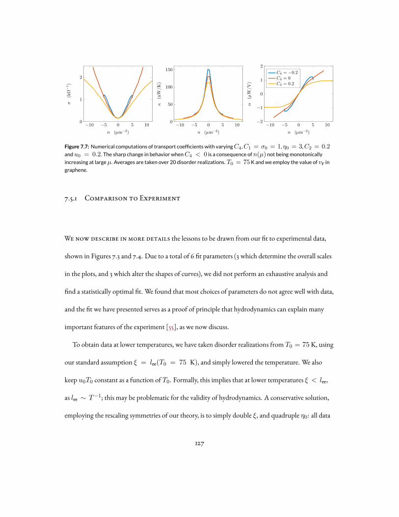
10 5 0 5 100

1

2

n (µm2)

(k1)

10 5 0 5 100

50

100

150

n (µm2)

(nW

/K)

10 5 0 5 102

1

0

1

2

n (µm2)

↵(µW

/V)

C4 = 0.2C4 = 0C4 = 0.2

Figure 1: testingFigure 7.7: Numerical computations of transport coefficients with varyingC4,C1 = σ0 = 1, η0 = 3,C2 = 0.2andu0 = 0.2. The sharp change in behavior whenC4 < 0 is a consequence ofn(µ) not beingmonotonically

increasing at largeµ. Averages are taken over 20 disorder realizations. T0 = 75K andwe employ the value of vF ingraphene.

7.5.1 Comparison to Experiment

We now describe in more details the lessons to be drawn from our fit to experimental data,

shown in Figures 7.3 and 7.4. Due to a total of 6 fit parameters (3 which determine the overall scales

in the plots, and 3 which alter the shapes of curves), we did not perform an exhaustive analysis and

find a statistically optimal fit. We found that most choices of parameters do not agree well with data,

and the fit we have presented serves as a proof of principle that hydrodynamics can explain many

important features of the experiment [55], as we now discuss.

To obtain data at lower temperatures, we have taken disorder realizations from T0 = 75K, using

our standard assumption ξ = lee(T0 = 75 K), and simply lowered the temperature. We also

keep u0T0 constant as a function of T0. Formally, this implies that at lower temperatures ξ < lee,

as lee ∼ T−1; this may be problematic for the validity of hydrodynamics. A conservative solution,

employing the rescaling symmetries of our theory, is to simply double ξ, and quadruple η0: all data

127

40 50 60 70 80 90

1

10

T (K)

(nW

/K)

Figure 1: testingFigure 7.8: A comparison of our numerical computation ofκ(T )with experimental results of [55] at the charge neu-

trality point (n = 0). The red data points are experimental data from [55], the blue curve is our disorder-averaged sim-

ulation (using identical parameters to Figure 7.4), and the green dashed curve is the perturbative predictionκ ∼ T 3

for comparison. Data is shown on a log-log scale. The yellow shaded region denotes where Fermi liquid behavior is

observed; the purple shaded region denotes the likely onset of electron-phonon coupling.

is exactly identical, except that for all data points taken in Figure 7.4, ξ > lee and η0 increases.

Figure 7.8 revisits the T -dependence in κ. Assuming that disorder is weak, we employ (7.18) and

(7.19) to determine the scaling of κ: since s ∼ T 2, ϵ + P ∼ T 3, ∂n/∂µ ∼ T , and the viscosity

dependence in τ is negligible, we obtain τ ∼ T and κ ∼ T 3. That numerics and experiment are

not consistent with this power law is a sign of the strong non-perturbative effects, and suggests that

observing power law signatures of hydrodynamics may only be possible in the cleanest samples: see

Figure 7.8. Figure 7.9 suggests that the sharp dependence in T observed in experiment is a conse-

quence ofC4 > 0 and is not a robust scaling regime.† As noted in [55], this dramatic T -dependence

of κ, in contrast with the very weak T -dependence of σ, at the Dirac point, is a tell-tale sign of hy-

drodynamics that is not captured by competing theories, such as the bipolar diffusion effect.

The fits to σ(n) and σ(T ) are not as good as the fits to κ. Nonetheless, our theory does help to

†For this particular simulation, the disorder becomes large enough at T ≲ 7.5K that disorder realizationswithC4 = 0.1 sometimes have unphysical thermodynamic behavior.

128

100 101 102

102

100

102

104

T (K)

(nW

/K)

C4 = 0C4 = 0.1

(T ) T 3

Figure 1: testingFigure 7.9: A comparison ofκ(T ) in simulations with varyingC4. We takeC0 = 1,C2 = η0 = 0.1,σ0 = 1,u0 = 0.1 (atT0 = 75K). At largeT both scenarios haveκ ∼ T 3; at lowerT the fluid withC4 > 0 undergoes a

dramatic drop inκ(T ), similar to that observed in experiment.

explain the slow growth in σ away from the Dirac point, as a consequence of a fluid with both non-

negligible viscosity and large disorder, as in Figure 7.6. Our simulations also correctly predict that

the conductivity is an increasing function of T , an entirely non-perturbative effect, in Figure 7.4.

This is at odds with predictions from kinetic theory in the Dirac fluid, which predict that σ(n =

0, T ) ∼ α−2eff should be decreasing with T due to the T -dependence in αeff [74]. Any residual

contact resistance [50] will also increase the growth rate of σ(n) away from the Dirac point, and as

such will be closer fit by our numerical results in Figure 7.3.

The most surprising thing about the fit is the large values of all coefficients, compared to previous

theories. For example, it is predicted [132, 67] thatC0 ≲ 3.4, and we findC0 ∼ 10. This is a direct

consequence of the large values of the density n over which the Dirac fluid is present (as measured

by where strong deviations from the Wiedemann-Franz law occur). The naive theoretical estimate is

that the Dirac fluid should not extend past about n ∼ 40 µm−2,† yet we see the Dirac fluid all the

†We have used theoretically predicted values ofC0 andC2 [67], and assumed that the Dirac fluid endswhen the µ-dependent contribution to s is comparable to the T -dependent contribution.

129

way to about n ∼ 200 µm−2; we will comment more on this issue shortly. As in non-relativistic

fluid dynamics, our hydrodynamic theory has a large number of rescaling symmetries (Appendix

B.2), and these rescaling symmetries turn out to lead to very large values for all hydrodynamic coeffi-

cients as a consequence of the large scale on the density axis in Figure 7.3.

Another consequence of this rescaling is a dramatically large shear viscosity: η0 ∼ 100. It is now

canonical to normalize this by the entropy density, and so the “proper units” to measure η in are

η0/C0 ≈ 10. This scaling is a consequence of a proposition [90] that strongly coupled theories

would have η/s ≈ ℏ/4πkB, or η0/C0 ≈ 1/4π. The viscosity is a helpful measure of the inter-

action strength in a theory; if the interactions are perturbatively controlled by a small parameter g,

then we expect η ∼ g−2; only when the interaction strength is large can η ∼ s, up to a prefac-

tor of order unity. Hence, coming close to saturating the bound of [90] is a signature that the fluid

is strongly interacting. Our estimate for η0/C0 is about 100 times larger than the bound of [90].

Smaller values of η/s ∼ 0.5ℏ/kB have been reported in other experiments in cold atomic gases [58]

and quark-gluon plasma [134]. The possibility of adding the Dirac fluid to a list of strongly interact-

ing quantum fluids is tantalizing, and a more direct measure of η in the Dirac fluid is of interest.

One possibility is that our bare coefficientsC0, η0 etc. are anomalously large because [55] has

measured the average charge density in the entire sample. However, some regions of the sample

(notably close to the contacts on the edges [135], or regions very close to impurities) may have such

large local values of µ0 that they are always in a Fermi liquid regime. So long as these Fermi liquid

regimes do not percolate across the entire sample, our hydrodynamic description of transport may

be quite reasonable in the bulk. However, these regions have a much smaller compressibility, and

130

so can absorb a lot of charge relative to a clean Dirac fluid. It may be that the total averaged charge

density is then not equal to the averaged hydrodynamic charge density, leading us to overestimate n.

Rescaling n → λnwould rescaleC0 → λC0 and η0 → λ2η0. Choosing λ = 0.2, in accordance

with our previous estimates on the regime of the Dirac fluid at T0 ∼ 75K, we obtainC0 ∼ 2 and

η0/C0 ∼ 2, which are both reasonable for a strongly interacting fluid.

As noted previously, we expect that future measurements in cleaner samples may give a wider

separation between lee and ξ. Together with a better understanding of edge effects and the charge

puddle profile, we expect this approach to lead to cleaner estimates ofC0,2,4, η0 and σ0.

7.6 Phonons in Graphene

Throughout this work we have neglected the effects of electron-phonon coupling in graphene

[51, 41]. In this section, we provide some brief qualitative comments on the role of electron-phonon

coupling in the experiment [55], and discuss signatures for future experiments.

Generically, phonons extract both energy and momentum from the electronic fluid, and in doing

so hamper a hydrodynamic description.† In graphene, the acoustic branch(es) of phonons have

dispersion relation [138]

ωac(q) ≈ ℏva|q| (7.29)

with va ≈ 2 × 104 m/s and so va ≪ vF. By considering conservation of energy and momentum†The hydrodynamic description of transport reduces to a diffusion equation for the conserved electrical

current. Historically, this was modeled via resistor networks [136, 137].

131

in electron-phonon scattering events, one finds that the phonon energies are negligible, and thus the

scattering event can be treated as elastic from the point of view of the electrons.

If only acoustic phonons couple to the electronic fluid, we may approximate that the momentum

conservation equation is modified, following the phenomenology of [87]:

∂µTµi ≈ F νi

extJν −T ti

τa. (7.30)

The latter term implies that the momentum of the electronic fluid degrades at a constant rate τ−1a ,

which we take to be

1

τa= BT a, (7.31)

where a > 0 and B > 0 are constants that are phenomenological. [138] computed their values

using kinetic theory and found a = 4 far from the Dirac point. This effect has been observed ex-

perimentally [40], but a is expected to change near the Dirac point. Following arguments similar

to [20, 138], we can estimate a by assuming a quasiparticle description of transport, and that the

dominant events are absorption or emission of a single phonon. Since acoustic phonons cannot ef-

fectively carry away energy, a Dirac quasiparticle of energy ϵ can scatter into∼ ϵ states. All phonons

with relevant momenta are thermally populated, and we estimate the scattering rate to be propor-

tional to the momentum of the phonon. Thus we estimate, using that the typical quasiparticle en-

ergy is ϵ ∼ T , a = 1 + 1 = 2.†

†As there is no large Fermi surface with µ ≫ kBT , no further corrections to a are necessary, as in usualmetals.

132

Assuming that the charge puddles are small and can be accounted for perturbatively, κ is approxi-

mately given by (7.2) at the Dirac point, with

1

τ≈ u2

2σq(ϵ+ P )

(∂n

∂µ

)2

+ BT a =Au2

T b+ BT a. (7.32)

Our analytic theory predicts b = 1. The contribution κ from electron-phonon coupling is negligi-

ble so long as

T ≪ T ∗ ≡(ABu2

) 1b+a

. (7.33)

Note that T ∗(u) is an increasing function – the weaker the disorder, the lower the temperature at

which electron-phonon coupling cannot be neglected in the Dirac fluid. The thermal conductivity

scales as

κ ∼

T 2+b T ≪ T ∗

T 2−a T ≫ T ∗(7.34)

If a > 2, we find phenomenology quite similar to that observed in [55], with κ(T ) growing non-

monotonically. We also find that

κ(T ∗) = C(T ∗)2−a, (7.35)

a result which can be tested in experiment by measuring T ∗ via the peak in κ for different samples.

The prefactor of this proportionality C may not be very sensitive to the particular sample, since it

is independent of u. Figure 7.10 shows a sketch of κ(T ), accounting for acoustic phonons, in three

samples with different disorder strengths u. This mechanism is also consistent with the fact that

133

T

Figure 1: testingFigure 7.10: A sketch ofκ(T ), accounting for coupling to acoustic phonons, for samples of graphenewith three differ-

ent amounts of disorder (measured byu). We takea = 3, b = 1 in this plot.

the cleaner samples in [55] had peaks in κ(T ) at lower temperatures, which suggests our proposed

mechanism for the non-monotonicity in κ(T ) is sensible. Although our perturbative quasiparticle-

based argument found a = 2 above, the presence of local charge puddles may increase the effective

value of a to somewhere between 2 and 4, and lead to κ(T ∗) be a decreasing function. A careful

analysis of electron-phonon coupling in disordered Dirac fluids is worth more study.

At higher temperatures, we expect optical phonons to couple non-negligibly to the electron fluid.

These phonons can exchange both energy and momentum effectively, and at this point we expect

the measured thermal conductivity to increase due to electron-phonon coupling. In [55], there is a

sharp upturn in κ(T ) at all densities at temperatures of 100 K, which is likely due to activation of

optical phonons in the boron nitride substrate [10].

134

7.7 Conclusions

We have developed a theory of transport in realistic hydrodynamic electron fluids near a

quantum critical point. This theory provides a substantially improved quantitative fit to κ(n) and

σ(n) simultaneously. We have further found reasonable quantitative fits to σ(T ) and κ(T ) at the

Dirac point, giving us valuable information about the mechanism of momentum relaxation beyond

the theory of [87].

Although we have managed to find fluids where the growth in σ(n) is quite slow, there are still

differences between the shape of σ(n) found numerically and in experiment. There are numerous

possibilities for residual discrepancies. One of the most important possibilities is that the disorder

is so strong that the full thermodynamic equation of state is necessary – in this paper, we have only

kept the three leading order terms. Alternatively, we may simply not have found the correct equa-

tion of state of graphene. A disorder profile more subtle than superimposed sines and cosines may

also be responsible for deviations with our theory, although our investigation into this possibility

suggests that other disorder profiles cause σ(n) to have more substantial density dependence. We

have assumed that the disorder profile is unaltered both by changes in T and in µ0. This is a very

strong assumption and need not be true. Finally, there may be other sources of momentum relax-

ation, such as out-of-plane distortions in the graphene lattice, or interactions with phonons. An

understanding of the aforementioned issues is an important future task, though may be quite chal-

lenging given the possibility that strong interactions in the Dirac fluid at T ∼ 70K may lead to the

135

failure of standard perturbative techniques. The most fruitful direction for resolving at least some of

these questions may be directly in experiments: for example, techniques to directly resolve the local

charge density on length scales≲ 10 nm are well known [53], and can shed light into the evolution of

µ0 as a function of T , as well as the spatial correlations in µ0.

Experimentally, it may be possible to generate samples of graphene with much weaker charge

puddles using suspended devices [139, 140]. Thermodynamic measurements can also be used to

determine the coefficientsC0,2,4, though these measurements are complicated by the presence of dis-

order, as we discuss in Appendix B.1. Nonetheless, measurements of the specific heat and compress-

ibility in the Dirac fluid will serve as valuable guideposts for future hydrodynamic models. Such

measurements have been made in the Fermi liquid [81], and their extension to the Dirac fluid form

the basis for worthwhile experiments.

Previous experiments which measured the ac conductivity [141] were not in the hydrodynamic

limit. Comparing the momentum relaxation time τ between measurements of κ, and a putative

Drude peak in ac transport, may provide a quantitative test of our theory. Studying magnetotrans-

port [87] may also be a fruitful direction in experiments. A theoretical discussion of transport at

finite frequency and magnetic field beyond the weak disorder limit will appear elsewhere. The ther-

mopower of graphene has recently been measured at T ∼ 200K [142], and it would be interesting

to measure σ, α and κ in the same sample in the Dirac fluid and compare with our hydrodynamic

formalism.

136

8Magneto-thermal transport

Extending thermal transport studies of two-dimensional systems into high magnetic fields

will facilitate a new wave of condensed matter experiments. Paired with electrical transport, thermal

techniques are sensitive to inter-particle scattering [60, 55, 89], quantum criticality [113, 74], charge-

less excitation channels [75, 143, 144, 145, 146, 147, 148], and can even be used to extract the entropy

137

of a system through the Gibbs relations [149]. Furthermore, Johnson noise and Joule heating are

particularly suited to magnetic experiments as, in the linear diffusive regime†, the ratio of the John-

son noise temperature (section 2.2) to the heating power P is insensitive to the current profile or

form of the conductivity tensor (section 4.3) while remaining quite sensitive to the ballistic, chiral

nature of quantum Hall states.

The techniques and methods applied in this chapter are described in detail in chapters 2 and 4.

8.1 Generalized transport coefficients

In the presence of a magnetic field, an electric field in a conductor can induce a current with

a component perpendicular to the applied fields. In general, the transport coefficients (σ, α, and κ)

take on a tensorial form (σ, α, and ˆκ) such that

J

q

=

σ α

T α ˆκ

E

−∇T

(8.1)

For systems with two spatial dimensions (x, y) and a perpendicular magnetic field, the transport

coefficient are 2 × 2matrices relating the local charge and heat current (J and q, respectively) to

the local electric field (E) and temperature gradient (∇T ). The electrical conductivity, defined as

the response of the charge current to an electric field with no thermal gradient, is simply given by†The linear diffusive regime assumes cooling is dominated by Wiedemann-Franz like diffusion, the elec-

trical conduction is sufficiently diffusive (not ballistic), and the temperature rise is small compared to theabsolute temperature scale.

138

σ. However, the thermal conductivity (κ) is not symmetrically defined as the response of heat cur-

rent to an applied temperature gradient in the absence of an electric field but instead defined in the

absence of a charge current. Thus,

κ ≡ ˆκ− T ασ−1α (8.2)

The form of the transport coefficients are constrained by a number of symmetries: The off diago-

nal elements of Eqn. 8.1 are related due to Onsager reciprocity† [150, 151] and rotational symmetry

requires all coefficients be antisymmetric — i.e all coefficients can be written in the form:

σ =

σxx σxy

−σxy σxx

(8.3)

For a degenerate Fermi liquid, it has been shown theoretically [151] and experimentally [152] that

the thermal-electric coefficient α is related to the electrical conductivity σ, component by compo-

nent, via the generalized Mott formula:

α = eL0Tdσdµ

(8.4)

where µ is the chemical potential andL0 = 13(πkB/e)

2 is the Sommerfeld value of the Lorenz

number [26]. However, in clean graphene samples inter-particle scattering breaks the assumptions

used to derive Eqn. 8.4 and violations of the Mott relation have been measured [142]. While a simi-

†Let α and ˆα be the two offdiagonal terms of eqn. 8.1. Time reversal symmetry and thus Onsager reci-procity demand αij(B) = αji(−B). But rotational symmetry forces α to be antisymmetric and thusαij(B) = −αij(−B) = αij(B). Where the last step was done by rotating π along an in plane axis.

139

lar theoretical treatment [151] has shown the validity of the generalized Wiedemann-Franz law

κ = L0T σ, (8.5)

several detailed calculations have predicted violations in graphene near landau quantization [153, 154,

155] and several more in the hydrodynamic regime [74, 60].

8.2 Classical Hall Effect

In low magnetic field or high carrier density, such that landau quantization does not signifi-

cantly modify the density of states, the tensorial form of σ can be calculated under the assumptions

of the classical Hall effect yielding:

σxx = σ01

1 + tan2(θH)

σxy = σ0tan(θH)

1 + tan2(θH)(8.6)

where

tan(θH) = −σ0e

B

n, (8.7)

σ0 is the zero field conductivity, n is the charge density, andB is the perpendicular magnetic field

strength.

140

Figure 8.1: Normalized voltage (upper) and temperature (lower) profiles resulting from Joule heating a uniform, square

conductor in the classical Hall regime for Hall angles 0 (le ), 45 (center), and 85 (right). The left and right sides ofeach profile correspond to electrical terminals with the the boundary conditions of constant voltage and temperature.

For θh = 0 current flows uniformily from left to right and the temperature profile is parabolic as discussed in

section 4.1. As the Hall angle is increased, the current bends and the location of the peak temperaturemoves closer to

the contacts. Near 90, all of the dissipation occurs at the contacts resulting in the formation of hot spots. All plots are

from finite element simulations [156]

141

As the field strength increases, the changing conductivity tensor results in a changing current dis-

tribution, which, in turn, results in a changing Joule heating profile and steady state temperature

distribution. Finite element simulations [156] illustrate how a magnetic field can affect the tempera-

ture and current profiles of a uniform, two-terminal conductor with the anisotropic σ and κ given

by Eqn. 8.6 and Eqn. 8.5, as shown in Fig. 8.1. Boundary conditions are chosen to match a typical

experiment where macroscopic electrical contacts serve as a thermal bath. In the absence of an ex-

ternal magnetic field, the current is uniform producing a parabolic temperature profile as discussed

in section 4.1. However, this simple calculation breaks down at finite field where current begins to

bend, resulting in an anisotropic temperature profile. At large magnetic fields, where the Hall an-

gle approaches 90, nearly all the dissipation occurs at two points near the contacts resulting in the

formation of hot spots. For a fixed Joule heating power, the spatial mean temperature of the sample

goes to zero as Hall angle is increased and the hot spot size approaches a singularity; the power of

Johnson noise measurements is that the measured Johnson noise temperature (section 2.2), TJN ,

naturally weights regions of higher local dissipation more such that as the dissipation approaches a

singularity, so too does the spatial weighting function for TJN — i.e. Johnson noise is sensitive to

the temperature of the hot spots.

142

Figure 8.2: Microscope image of the graphene device used in this chapter. Multiple devices of various geometries are

made from the same hBN-graphene-hBN stack on an insulating sapphire substrate. The two-terminal device used in

this chapter is the second from the left and has a dimension of 4µm× 4µm. A lithographically defined local top gate

is used to control carrier density.

8.3 Graphene characteristics

Monolayer graphene is mechanically exfoliated, encapsulted with hexagonal boron

nitride (hBN), and contacted along its one dimensional edge [50] to form a square, two-terminal

device (4 µm × 4 µm). These dimensions are chosen as a balance between the requirements that

the device be longer than the electronic mean free path yet short enough that Wiedemann-Franz

cooling dominates over electron-phonon cooling, as discussed in chapter 4. Samples are fabricated

on insulating sapphire substrates with a local top gate to electrostatically control carrier density as

shown in Fig. 8.2. The gate capacitance is measured using the integer quantum Hall effect. The low

temperature, two-terminal resistance varies between 0.2 and 4.3 kΩ by varying the top gate±5 V ,

143

Figure 8.3: DC resistance of the graphene device at zeromagnetic field as a function of carrier density controlled via

an electrostatic top gate. Gate capacitance is measured using the integer quantumHal effect.

corresponding to a carrier density of∼ ±1.6 × 1012cm−2, as shown in Fig. 8.3. The conductivity

minimum is attained for a top gate voltage Vg = −430mV corresponding to an intrinsic electron

doping of 1.4×1011cm−2. The FWHM of the resistance is 5×1010cm−2 with a minimum carrier

density of nmin ≈ 1.2× 1010cm−2, where nmin is defined in accordance with chapter 6.

The sample is cooled to 1.7K by a variable temperature, 4He vapor cryostat (Appendix A.2

equipped with a 14 T superconducting magnet. The DC two-terminal resistance is measured up

to 13 T and shown in Fig. 8.4. Integer quantum Hall states are present at fields as low as 0.5 T

and the ν = 1 symmetry broken state appears at high field. By analyzing the resistance values of

the quantum Hall plateaus, the contact resistance is estimated to vary between 50 and 170Ω as a

function of density at 1.7K . Low contact resistance is vital to Johnson noise thermometry as any

dissipation that occurs outside of the sample will lead to unwanted Johnson noise which can de-

144

Figure 8.4: Two-terminal DC resistance of amonolayer graphene device at 1.7K . (le ) Resistance is shown on a log

scale as a function of carrier density and perpendicular magnetic field strength. (top right) and (bo om right) showcuts at constant density and field, respectively.

grade the measurement. Using these estimates for the contact resistance, we can estimate the zero

field conductivity and thus the Drude mobility and elastic mean free path which vary between

0.2 − 2 × 105 cm2/V s and 200 − 650 nm, respectively, as a function of density, as shown in

Fig. 8.5.

8.4 Electrical noise in high fields

Varying by over two orders of magnitude, the DC resistance of the graphene device must

be impedance matched using a wide dynamic range matching network. As described in detail in sec-

tion 2.6, an on chip, two-stage LC tank circuit in a low-pass configuration is used to transform the

145

Figure 8.5: Estimated Drudemobility and elastic mean free path of the graphene device used in this chapter as a func-

tion of electron density at 1.7K . Estimates aremade from the two-terminal conductance at zeromagnetic field

assuming a contact resistance estimated from the resistance of the integer quantumHall plateaus. The Drude estima-

tion breaks down near the charge neutrality point where the carrier density is not simply given by the charge density

divided by the electron charge

sample impedance to near 50Ω. To meet the strict requirements of multi-stage matching, the device

was built on an insulating sapphire substrate and surface mount inductors and capacitors were di-

rectly soldered to a coplanar waveguide. All inductive elements were air-core as to be magnetic field

insensitive and used gold leads which facilitated the direct connection of the graphene sample via

wirebond, as shown in Fig. 8.6.

A vector network analyzer (VNA) can be used to test the high frequency coupling to the device.

As the sample resistance changes, different regions of the noise spectra are efficiently coupled into

the measurement circuit, as shown in Fig. 8.7. At a DC resistance of 1 kΩ the noise bandwidth of

the matching network is∼150MHz and>3 dB coupling continues for resistances above 100 kΩ.

Quantifying the coupling in terms of a noise measurement for a circuit as detailed in section 2.4, we

146

Figure 8.6: Custom sample package used tomeasure graphene thermal conductance in highmagnetic fields. The

graphene device is placed on an insulating sapphire substrate which is mounted to the sample package using double-

sided Kapton tape. The sample is thenwire bonded directly to an air-core surfacemount inductor which is part of a

two-stage LC tank circuit used to impedancematch the high resistance device. The output of the network is soldered

directly to a coplanar waveguide which terminates in a high frequency SMP connector. An RF shield then encloses the

the device which can be loaded into a cryostat.

Figure 8.7: Reflection coefficient as a function of frequency and grapheneDC resistance. The two-stage LCmatching

circuit is designed to couple a wide dynamic range of resistances allowing the continual measurement of graphene

from zeromagnetic field to quantumHall states. When optimally matched atR ≈ 1kΩ, the circuit has a noise band-

width of∼150MHz. As detailed in section 2.6, the high frequency solution of the two-stage network is intentionallymoved to a higher resistance creating a wider dynamic range.

147

Figure 8.8: Generalize gain and noise temperature, as defined in section 2.7 and Eqn. 8.8, for the graphene device and

matching network shown above. Gain is maximize, and noise temperature is minimizedwhen the device is optimally

matched at 1 kΩ. This data is collected by varying the carrier density of graphene at three different magnetic field

values, 0, 1, and 13T . All data collapses onto the same line indicating thematching circuit is field insensitive and

depends only upon the grapheneDC resistance.

can write the measured output voltage as

Vout = G(Γ )(T + Tn(Γ )). (8.8)

Calibration as outlined in section 2.8 yields G(Γ ) and Tn(Γ )which are plotted as a function of the

DC resistance in Fig. 8.8. We find the calibration parameters to depend only upon the graphene DC

resistance and not upon temperature or magnetic field, indicating the matching network is stable

over the parameter range of our measurement. With the device matched and the circuit calibrated,

we can measure the total output noise from the sample (Fig. 8.9). During the course of an experi-

ment it is common for the background noise Tn to fluctuate on a long time scale (e.g. hours); thus

to reach the desired sensitivity it is necessary to perform differential measurements, as described in

chapter 4, by sinusoidally varying the a Joule heating current and measuring the cosinusoidal elec-

148

Figure 8.9: DC voltage proportional to the total noise emitted into themeasurement bandwidth, as defined by Eqn. 8.8,

from a graphene device as a function of carrier density andmagnetic field at 1.7K . Horizontal streaks appear in

the data as the system noise temperature fluctuates over the course of the experiment illustrating the need for the

differential measurements performed in section 8.5.

tronic temperature rise with a lock-in amplifier.

8.5 Magneto-thermal conductance

While injecting heat into the electronic system, the steady state temperature rise pro-

vides information on how efficiently the system transports thermal energy to the bath. Applying the

methodology of chapter 4, a differential heating current applies a peak power of P0 to the graphene

device and the peak-to-peak differential Johnson noise temperature∆TJN is measured†. When

†Calibration of these differential measurements only requires the use of generalized gain, G. Any fluctua-tions in the background noise are averaged out and Tn is only important in that it determines how long youmust average to reach the desired precision.

149

Figure 8.10: Differential Johnson noise temperature rise of a graphene device in response to a differential heating

power of 0.4nW as a function of carrier density andmagnetic field atTb = 1.7K . At low field and high density, the

electronic thermal conductivity is high in accordance with theWiedemann-Franz law resulting in a small temperature

rise. As the field increases, so too does the electrical resistance and thus the thermal resistance and the steady state

temperature rise. However, the appearance of quantum effects results in a drastic reduction of∆TJN due to the

ballistic nature of the conduction channel.

the device’s thermal conductance is large,∆TJN is reduced, while an enhancement of∆TJN sig-

nifies a reduction of the thermal conductance. Fig. 8.10 shows the differential (quasi-steady state)

electronic temperature rise of a square, two-terminal graphene device (described in section 8.3) for

a heating power P0 = 0.4 nW. Much of the qualitative heating behavior can be understood via

the Wiedemann-Franz law; at low field and high density∆TJN is found to be small, as the electrical

conductivity (and therefore the thermal conductivity) is large, while at higher fields,∆TJN is larger

due to magnetoresistance affecting the thermal conductivity. At lower density, we find quantum

oscillation in the thermal signal and a drastic reduction of∆TJN in quantum Hall states.

To analyze this quantitatively, we can define a thermal resistance (Rth) as the inverse of the ther-

150

mal conductance defined in chapter 4,

Rth ≡ ∆TJN

P0(8.9)

Its important to note thatRth is not the traditional thermal resistance, which describes the total

heat current flowing through a material in response to a spatial temperature gradient; it is instead a

generalized thermal resistance describing the heat power transferred between the electronic system

and the bath under Joule heating. For a diffusive system† dominated by Wiedemann-Franz elec-

tronic cooling, the thermal resistance in the linear response regime is given by:

Rth =R

12L Tb(8.10)

whereL is the Lorenz ratio and Tb is the bath temperature. Eqn. 8.10 is derived in section 4.3 and

holds under the following assumptions:

1. Heat conduction is provided entirely by electron diffusion of the form κ ∝ σ, where theconstant of proportionality is defined asLTb by convention

2. The transport coefficients are spatially uniform

3. The device has only two electrical terminals which serve as thermal reservoirs and sources ofJoule heating current

4. The elastic mean free path of the charge carriers is shorter than all other relevant length scalesin the system

†Here a diffusive system is defined as one where the elastic mean free path of charge carriers is smaller thanall other relevant length scales in the problem

151

Figure 8.11: (upper) Comparison of the thermal resistanceRth ≡ ∆TJN/P0 (blue) and the electrical resistanceR(red) for monolayer graphene hole doped away from the charge neutrality point (n ≈ −1.6 × 1012cm−2). (Insets)show the expected classical Hall temperature profiles for select Hall angles from finite element simulation [156] under

the assumption of theWFL. (lower) Themeasured Lorenz ratioL ≡ (R/Rth)(1/12Tb) normalized to the Sommer-

feld value. For magnetic fields below a few Tesla,Rth tracksR, but at high field, the behavior ofRth deviates sharply

from that ofR.

152

Figure 8.12: (upper) Comparison of the thermal resistanceRth ≡ ∆TJN/P0 (blue) and the electrical resistance

R (red) for monolayer graphenewith a carrier (hole) density ofn ≈ −1.2 × 1011cm−2. At low field,R increases

whileRth decreases with quantum oscillations appearing in the thermal data around 0.3T . In the ν = 2 quantum

Hall state, the electrical data shown a plateau at the expected 12h/e

2 while the thermal resistance drops close to zero.

At themagnetic field strength corresponding to other filling fractions, ν = 10, 6, 1, and 2/3, the thermal signal shows

a similar drop toward zero even though the electrical plateaus are not present. (lower) Themeasured Lorenz ratio

L ≡ (R/Rth)(1/12Tb) normalized to the Sommerfeld value.

Fig. 8.11 comparesR andRth for graphene with a large carrier density (n ≈ −1.6 × 1012cm−2)

as a function of magnetic field strength at 10K . For fields up to a few Tesla, we find that, whileRth

qualitatively tracks the field dependence ofR, the measured Lorenz ratio,L ≡ 112 Tb

(R/Rth),

has a small field dependence, even in the so-called “classical” regime, in stark contrast to the pre-

dictions of Eqns. 8.10 and 8.5. In high field, where landau quantization becomes relevant, the be-

havior ofRth begins to significantly deviate from that ofR, eventually decreasing with field and

tending towards zero. At low density this behavior is even more pronounced as quantum effects

enter as low as 0.5 T . Fig. 8.12 shows similar measurements to Fig. 8.11 for a lower carrier density of

153

n ≈ −1.2 × 1011cm−2. Unlike the high density data shown in Fig. 8.11, at low density,Rth de-

creases with magnetic field for low fields even thoughR increases. For all densitiesLmonotonically

increases with field until quantum oscillations are seen. At fields and densities where the electrical

data shows well developed plateaus, the thermal signal drops to near zero and the measuredL di-

verges as a result of the ballistic nature of quantum Hall states. In fact, this combination of Johnson

noise thermometry and Joule heating is particularly suited to the detection of quantum modulations

of the density of states; this is readily seen in Fig.8.12 where, although not fully developed electrically,

the thermal signal shows several more integer states, including the symmetry broken state ν = 1,

and the fractional state ν = 2/3. The sensitivity of this technique to quantum effects results from

its intimate connection to changes in entropy and carrier thermalization length. Fig. 8.13 shows the

entire thermal fan diagram at Tb = 1.7K .

8.6 Cyclotron radius

Given the apparent violation of Eqn. 8.10 at finite magnetic field, it stands to reason that one

of the four assumptions listed above must be violated in graphene. The most obvious of which is

the assumption that the elastic mean free path is shorter than all other relevant length scales. In the

presence of a magnetic field, electrons in two-dimensional conductors travel along cyclotron orbits

of radius

rc =m∗vFe B

(8.11)

154

Figure 8.13: Themeasured Lorenz ratioL ≡ (R/Rth)(1/12Tb) of a square graphene device normalized to the

Sommerfeld value as a function of carrier density andmagnetic field atTb = 1.7K . Color axis shown on a log scale.

QuantumHall states appear as lines of large Lorenz number

where vF is the Fermi velocity andm∗ is dynamical mass of the charge carrier. Unlike traditional

conductors with parabolic dispersions, the dynamical mass graphene is a function of the Fermi en-

ergy (EF ) and given by the relativistic form

m∗ = EF /v2F (8.12)

= ℏ√πn/vF (8.13)

155

Figure 8.14: Characteristic cyclotron radius l∗(n) at whichL begins to deviate fromL0. Large cyclotron radius cor-

responds to small magnetic field. (insets) plot two representative examples of how l∗ is extracted; a linear fit to the logofL vs cyclotron radius (rc) is extrapolate to the constant, low field valueL(B ≈ 0). Red shaded region represents50% convince intervals of the fits. These values can be directly compared to the quasiparticle elastic mean free path

estimated by the zero field conductance in Fig. 8.5.

thus the cyclotron radius can be written as a function of carrier density and magnetic field, as:

rc =ℏ√πn

e B(8.14)

= l2B√πn (8.15)

where lB =√ℏ/eB is the magnetic length.

As we increase magnetic field for a fixed carrier density, we can quantitatively define a character-

istic cyclotron radius (l∗) at whichL begins to deviate from /sL0 by extrapolating a linear fit of the

log ofL(rc) to the constant low field valueL(B ≈ 0). The insets of Fig. 8.14 show two represen-

tative examples of this procedure. l∗(n) is the relevant magnetic length at which we see violations

156

of eqn. 8.10 for a given density. The main panel of Fig. 8.14 plots l∗ as a function of electron density.

The values found should be quantitatively compared to the elastic mean free path of the charge car-

riers which is estimated from the zero field conductance in Fig. 8.5. Essentially, the mean free path

imposes a length cutoff for variations of the local temperature — i.e the temperature cannot equili-

brate at scales shorter than the mean-free path, since over these length scales electrons move ballisti-

cally. The strong agreement between the data in Figs. 8.14 and 8.5 (rms normalized error of 23%) is

evidence that the deviations ofL fromL0 are due to relevant dynamics occurring on a length scale

where electrons are ballistic. This is taken to an extreme in the limit of quantum Hall where conduc-

tion occurs only on ballistic edge channels and hence the measured Lorenz ratio diverges.

157

ARF cryostats

All experiments reported in this thesis were performed in one of three cryostats, each wired

for high frequency measurements. A custom sample mounting board was machined from copper

laminated PTFE (Rogers Corp, RT/duroid®), as shown in Fig. A.1. Five coplanar waveguides, with

characteristic impedance 50Ω, are milled into the circuit board along with 14 DC lines and a DC

158

Figure A.1: Images of the circuit board used tomount samples. (Le ) sample is placed in the copper free area in the

center of the board. Five coplanar waveguides aremilled along the outer ring. 14 DC lines with bonding pads and a DC

ground aremachined on one end. (Right) the backside of the circuit board where each RFwaveguide is soldered to anSMP connector and all DC lines are soldered to the pins on a “NanoD” connector.

ground. Each RF waveguide ends in a through board SMP male connector while all DC lines and

the DC ground connect to a through board “NanoD” connector. The entire circular board mea-

sures 1 inch in diameter allowing it to lowered into the small bore of a superconducting magnet.

The sample and SMD inductors/capacitors are fixed to the board using double sided Kapton

tape and all componets are wired together using either solder or direct wirebonding. Fig. A.2 shows

an example of a double-stage match network connected using only wirebonds. In practice, alu-

minum wire bonds have difficulty bonding to the soft pads of the SMD capacitors and so often

solder is used for these parts. Once connected, the sample is sealed in an RF tight copper box which

can loading into any of the three cryostats described below.

159

Figure A.2: Example of components mounted on our circuit board. In this case, 2 inductors (blue elements with gold

leads), 2 capacitors (grey elements with silver leads), and one resistor (blue element with silver leads) forming a two-

stage LCmatching network. Components are secured using double-sided Kapton tape and connected using aluminum

wirebonds.

A.1 Janis

The experiments discussed in chapters 5 and 6 were performed in one of two 4He closed

cycle Janis SHI-4 cryocoolers located at Raytheon BBN Technologies and Harvard University. The

Harvard system is shown in Fig A.3 and operates with the sample in vacuum over a continuous tem-

perature range of 2.8 − 320K . Custom copper thermalization plates were machined to thermally

anchor SMA bulkheads at 50K and base temperature. Solid, semi-rigid coaxial cables with cop-

per inner and outer conductors are run through the system. Often low-pass filters are placed at the

50K stage to help reflect high frequency thermal noise from room temperature. A heater and ther-

mometer are mounted on the sample stage to control and measure the bath temperature using a

160

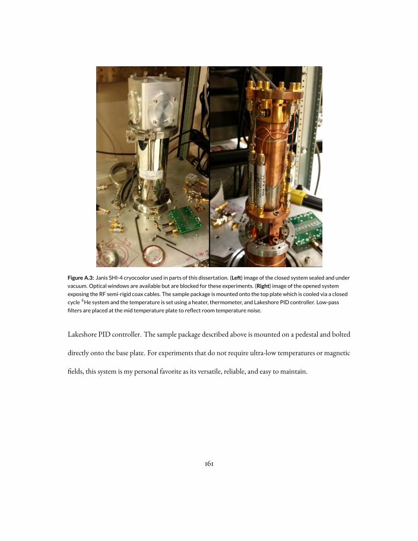
Figure A.3: Janis SHI-4 cryocoolor used in parts of this dissertation. (Le ) image of the closed system sealed and under

vacuum. Optical windows are available but are blocked for these experiments. (Right) image of the opened system

exposing the RF semi-rigid coax cables. The sample package is mounted onto the top plate which is cooled via a closed

cycle 4He system and the temperature is set using a heater, thermometer, and Lakeshore PID controller. Low-pass

filters are placed at themid temperature plate to reflect room temperature noise.

Lakeshore PID controller. The sample package described above is mounted on a pedestal and bolted

directly onto the base plate. For experiments that do not require ultra-low temperatures or magnetic

fields, this system is my personal favorite as its versatile, reliable, and easy to maintain.

161

Figure A.4: Sample packagemounted to the custom adapter made for theOxford cryostat. Adapter has twomachined

holes to house a heater and thermometer. Entire package is then affixed to the end of a long SS thin-walled tube and

lowed into theOxford VTI.

A.2 Oxford

The Oxford brand cryostat, used for the bulk of chapter 8, is a wet 4He system with a variable

temperature insert (VTI) capable of operating from 1.7−300K . It houses a 14 T superconducting

magnet with a relatively small∼1.1 inch bore. The sample is inserted into the VTI and cooled via

cold 4He vapor which is held at a fixed temperature by a heater and thermometer located at the

vapor inlet and controlled by a Lakeshore PID controller.

The sample package described above is attached via non-magnetic SS screws to a custom copper

adapter, as shown in Fig. A.4. This custom adapter was machined to house a Cernox® thermometer

(Lakeshore AA package) and resistive cartridge heater. The entire package can then be affixed onto

the end of a long SS thin-walled tube and held in place by a set screw, as shown in Fig. A.5. A cop-

162

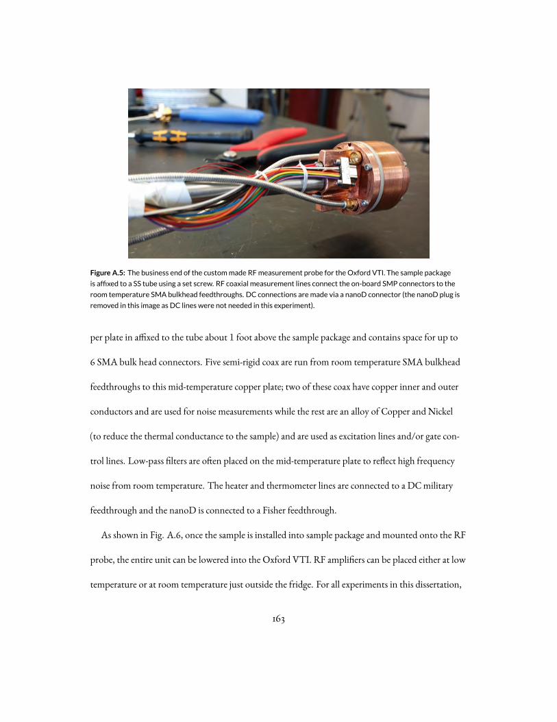
Figure A.5: The business end of the custommade RFmeasurement probe for theOxford VTI. The sample package

is affixed to a SS tube using a set screw. RF coaxial measurement lines connect the on-board SMP connectors to the

room temperature SMA bulkhead feedthroughs. DC connections aremade via a nanoD connector (the nanoD plug is

removed in this image as DC lines were not needed in this experiment).

per plate in affixed to the tube about 1 foot above the sample package and contains space for up to

6 SMA bulk head connectors. Five semi-rigid coax are run from room temperature SMA bulkhead

feedthroughs to this mid-temperature copper plate; two of these coax have copper inner and outer

conductors and are used for noise measurements while the rest are an alloy of Copper and Nickel

(to reduce the thermal conductance to the sample) and are used as excitation lines and/or gate con-

trol lines. Low-pass filters are often placed on the mid-temperature plate to reflect high frequency

noise from room temperature. The heater and thermometer lines are connected to a DC military

feedthrough and the nanoD is connected to a Fisher feedthrough.

As shown in Fig. A.6, once the sample is installed into sample package and mounted onto the RF

probe, the entire unit can be lowered into the Oxford VTI. RF amplifiers can be placed either at low

temperature or at room temperature just outside the fridge. For all experiments in this dissertation,

163

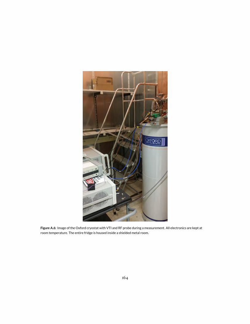
Figure A.6: Image of theOxford cryostat with VTI and RF probe during ameasurement. All electronics are kept at

room temperature. The entire fridge is housed inside a shieldedmetal room.

164

all electronics were kept outside the fridge at room temperature.

A.3 Leiden

For ultra-low temperature experiments, a dry dilution refrigerator from Leiden cryogenics

was used, as shown in Fig. A.7. This entirely closed cycle system has a base temperature of∼10mK

and a large bore (∼6 inches) magnet with a maximum field strength of 5 T . To facilitate fast experi-

ment turn around times, it is equipped with a top loading probe which can bring a sample down to

base temperature in a few hours. To access the cold plates for maintenance or install a longer term ex-

perimental setup, the fridge vacuum shields can be removed with the help of 4 electrically controlled,

mechanical legs, as shown in Fig. A.8.

Inside, the system consists of two independent vacuum chambers and five large gold plated cop-

per plates thermally isolated from each other. The first and second plates are cooled by an electrically

isolated pulse tube and, during operation, typically run at 50K and 4 − 5K , respectively. The

outer vacuum chamber (OVC) contains the entire 50K plate and the upper half of the 4K plate

along with two sorption pumps and two heaters. The bottom half of the 4K plate forms the top of

the inner vacuum chamber (IVC) which is sealed with a Kapton o-ring. Four large SS tubes connect

into the IVC to allow probes to enter; the central port is used for the main probe (described below),

one of the secondary ports is used to bring in 16 RF coaxial cables, and the other two are held in

reserve for future expansions. The bottom half of the 4K plate also contains 2 sorption pumps

165

Figure A.7: Image of the closed cycle dilution refrigerator made by Leiden cryogenics installed in the Kim lab. The

insertable, top-loading probe is seen in the upper half of the image enclosed in flexible bellows. The system sits on four

electrically controlled, mechanical legs to lift the system for easymaintenance.

166

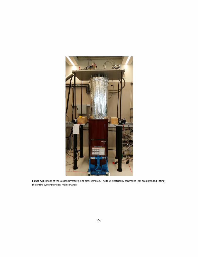
Figure A.8: Image of the Leiden cryostat being disassembled. The four electrically controlled legs are extended, lifting

the entire system for easymaintenance.

167

which pump out the IVC and can be heated (via internal heaters) to release exchange gas into the

IVC. The third plate contains the still/impedances and typically operates at a temperature of around

0.8K . The still has an on-board heater allowing the He mixture evaporation rate to be controlled†.

The 5 T magnet is bolted onto the still plate and thus operates at the still temperature, as shown in

Fig. A.9. While running the magnet it is therefore import to watch the still temperature. The fourth

plate has no direct cooling mechanism but serves as both a radiation shield and a location to mount

the heat exchangers for the dilution circuit; during operation is typically sits around 100mK . The

fifth and final plate contains the dilution mixing chamber and includes a long tail that dips into the

magnet bore. Fig A.10 shown a close up of the entire IVC (lower 4 plates).

To perform RF measurements, one of two options is available: firstly, if the number of cold mi-

crowave elements is small, all circuitry can be installed directly onto the insertable probe‡, secondly,

the microwave components can be installed into the main body of the fridge and connected to the

sample via internal lines and an RF “clicking mechanism” that couples to the probe. As shown in

Fig. A.11, internal microwaves lines connect each stage; 14 coaxial excitation lines with copper/nickel

alloy inner and outer conductors and 2 measurement lines with superconducting niobium-titanium

inner and outer conductors run between the stages. All excitation lines are attenuated at each stage

to thermalize the electronic temperature (reduce the Johnson noise to the appropriate level).

The insertable, top-loaded probe is shown in Fig. A.12 with the electronically controlled bellows

†In principle, raising the evaporation rate results in more cooling power and a high base temperature butin practice the rate must be adjusted to find the proper balance for a given setup.

‡The cooling power of the probe is limited by the thermal contact to the cold plates so caution must betaken if active elements such as amplifiers are required.

168

Figure A.9: Image of the 5T superconductingmagnet, made by AmericanMagnet Inc, installed in the Leiden system.

Themagnet is thermalized to the still plate and thus operates near 1K .

169

Figure A.10: Close up of the Leiden IVC plates. Starting from the top, the shown plates are the 4K , still, 100mK ,

andmixing chamber plates. The still is the silver piece seen on the left side of the imagemounted on the top side of the

still plate. Image taken in Leiden, Netherlands while constructing the fridge. At the bottom of the image, the “tail” that

extends down into themagnet bore can be seen

170

Figure A.11: Image of themicrowave lines inside in the body of the Leiden cryostat. Shown here are the 14 excitation

lines connecting the still plate to themixing chamber plate attenuated at every stage. Not shown are the 2 supercon-

ductingmeasurement lines installed alongside these without attenuators.

171

lowered. The probe holds up to 8 high frequency lines and over 24 DC lines if needed. For each of

the five temperature stages in the main fridge body, the probe has a corresponding set of pneumatic

expanding thermalization plates; once the probe is fully inserted, these plates expand to thermally

sink each stage of the insert to a stage in the main body†. A location to place 8 SMA bulkheads is

built into every temperature stage. Attached to the final (mixing chamber) stage in a long extension

arm which reaches into the magnet bore. The sample is placed at the end of this extender.

For the experiments in this dissertation, the number of cold microwave elements was small and

thus all components could be installed onto the probe itself. Fig. A.13 shows an example of one the

these circuits. A cold amplifier‡ is mounted to the 4K stage and a bias-tee along with two direc-

tional couples are attached to allow for DC transport and RF reflection/gain measurements.

At the bottom of the probe (where the sample sits) is a plate with 16 SMP (smooth barrel) con-

nectors pointing downward that fit into matching connectors installed in the main fridge body.

When the probe is fully inserted, these connectors make an RF connection between the probe and

the main body of the Leiden allowing experiments that require more complicated circuitry to use

the ample space and cooling power of the main fridge. Fig. A.14 shows an image of the underside of

this “clicking” mechanism where 16 SMA connectors can be used to probe the sample.

†While most stages sink well, the 50K stage is in the OVC and, therefore, has to thermalize through a SStube.

‡Cal-Tech CITLF3

172

Figure A.12: Image of the insertable, top-loading probe built for the Leiden dilution refrigerator with the retractable

bellows lowered. Each gold plated copper sectionmechanically expands once inserted to thermalize to a stage in the

main fridge body. Near the bottom of the probe, and extender is seenwhich, during operation, contains the sample and

is lowered into themagnet bore.

173

Figure A.13: An image of amicrowave noisemeasurement circuit installed on the Leiden probe. A low noise amplifier

is mounted to the 4K plate and a bias-tee along with two directional couples are attached. This setup allows RF

reflection and gainmeasurements of the sample and amplifier, respectively, as well as DC transport and RF noise

measurements.

174

Figure A.14: Image of the underside of the “clicking” mechanism in the Leiden located in themain body of the fridge

at the end of the tail that extends into themagnet bore. 16 SMA connectors are available and correspond to the 16

SMP connectors on the end of the probe. When the probe is fully inserted, these connectors form an RF connection

between the probe and themain fridge body.

175

BHydrodynamic framework

B.1 Thermodynamics

In this appendix and in every subsequent appendix, we will work in units where ℏ = kB =

vF = e = 1. It is straightforward using dimensional analysis to restore these units.

We consider the equations of state of the relativistic plasma in a relativistic strongly interacting

176

fluid in d = 2. Without specific microscopic details, these are very general facts about relativistic

plasmas without an intrinsic mass scale (or gap). The discussion generalizes straightforwardly to

other d. The only relevant energy scales are the temperature T and the chemical potential µ. We

have the general Gibbs-Duhem relation:

ϵ+ P = µn+ Ts, (B.1)

where ϵ is the energy density, P is the pressure, s is the entropy density and n is the charge density

(n = 0 at the particle-hole symmetric Dirac point). In a relativistic fluid,

P = T 3F(µ

T

)(B.2)

for some dimensionless functionF . Thermodynamic identities imply that

n =∂P

∂µ= T 2F ′

(µ

T

)(B.3a)

s =∂P

∂T= 3T 2F − µTF ′

(µ

T

)=

3P − µn

T. (B.3b)

Combining (B.1) and (B.3) we obtain

ϵ = 2P. (B.4)

The hydrodynamic description is only sensible for µ ≪ T – for µ ≫ T the standard Fermi liq-

uid description applies. Furthermore, the equations of state of the Dirac fluid are charge conjugation

177

symmetric, implying thatF is an even function of µ. So we Taylor expand:

F(µ

T

)≈ C0

3+

C2

2

(µ

T

)2+

C4

4

(µ

T

)4. (B.5)

Using (B.3):

n = C2µT + C4µ3

T, (B.6a)

s = C0T2 +

C2µ2

2− C4µ

4

4T 2. (B.6b)

We also require thatC0, C2 ≥ 0, so that s ≥ 0 and that n/µ is positive as µ → 0, as it should be.

B.1.1 Thermodynamics of Disordered Fluids

Already at this point we can make interesting predictions about the thermodynamics of the

strongly interacting hydrodynamic regime in graphene. For concreteness, let us suppose that the

background chemical potential is

µ0(x) = µ0 + µ(x), (B.7)

with µ0 a constant and µ a zero-mean random function; for simplicity, suppose that µ is evenly

distributed about zero, and has a disorder correlation length of ξ ≳ lee, so that the hydrodynamic

178

description applies. In this case, spatially averaging over µ0, we find

⟨ϵ⟩ = 2C0

3T 3 + C2T

(µ20 +

⟨µ2

⟩)+

C4

2

(µ40 + 6µ2

0

⟨µ2

⟩+

⟨µ4

⟩)+ · · · . (B.8)

The · · · denotes higher order terms in the equation of state that we have neglected. A similar expres-

sion can be found for the charge density:

⟨n⟩ = C2T µ0 +3C4

Tµ0

⟨µ2

⟩+ · · · . (B.9)

Let us focus on a clean limit where µ is very small relative to T . Let us also assume that we are

close to the Dirac point, so that onlyC0 andC2 terms need to be kept. Thermodynamics then gives

tight constraints on the behavior of measurable quantities: specific heat and compressibility, in an

experimentally testable regime, due to the ability to easily tune both T and µ0 (the average charge

density) experimentally. In the limit above, the (spatially averaged) compressibilityK is

1

K=

∂⟨n⟩∂µ

= C2T. (B.10)

where as before, we use ⟨· · · ⟩ to denote a uniform spatial average. Note that the independence ofK

to µ0 and µ is simply a consequence of the fact that we did not expand (B.5) to quartic order. The

spatially averaged specific heat

c =∂⟨ϵ⟩∂T

= 2C0T2 + C2

(µ20 +

⟨µ2

⟩). (B.11)

179

The experimental consequence of this result is as follows. Very close to the Dirac point, we expect

thatK is approximately constant. Restoring all dimensional prefactors, we can therefore set

C2 ≈(ℏvF)2

KkBT(B.12)

and re-write

c ≈ 2C0k3BT

2

(ℏvF)2+ 2

µ20 +

⟨µ2

⟩KT

≈ 2C0k3BT

2

(ℏvF)2+ 2

⟨µ2

⟩KT

+2Kn2

T. (B.13)

We thus see that the quadratic dependence in c(n) gives us an independent measurement ofK

through a measurement of the heat capacity. In principle, a quadratic polynomial fit to c(n) thus

determines bothK andC0, up to the residual effects of disorder, which will lead to an overestimate

ofC0. Repeating measurements ofK directly, as well as c(n) at different T , provide non-trivial

checks on the above theory. It is important to note that this argument does not rely on the validity

of hydrodynamics, only that graphene is gapless, µ0 ≪ T , and that µ is very small. Of these three

requirements, the last poses the biggest experimental hurdle.

In the above argument, there is no reason a priori why to truncate the Taylor expansion to neglect

C4 and higher order corrections, beyond appealing to the weak disorder limit. In particular, inclu-

sion ofC4 complicates our ability to obtain an accurate measure of µ0 from n. The argument above

is simply meant to give a flavor for the constraints on measurable quantities imposed by scale invari-

ant thermodynamics. A more systematic treatment is likely necessary to make quantitative contact

180

with future experiments.

B.2 Rescaling Symmetries of dc Transport

Solutions to (7.14) are invariant, up to global rescalings, under certain rescalings of the lin-

earized hydrodynamic equations of motion. These symmetries are, assuming λ > 0 is a constant

scaling parameter:

η → λ2η, x → λx; (B.14a)

η → λη, σ → λσ, α → λα, κ → λκ, P → λP ; (B.14b)

α → λα, κ → λ2κ, η → λ−2η, µ0 → λµ0, C2 → λ−2C2, C4 → λ−4C4, etc.;

(B.14c)

α → λα, κ → λκ, σ → λσ, η → λ−1η. (B.14d)

Everything not listed is invariant. ζ and η have the same scalings, as do σ and σq, and so we have

only listed some of these parameters.

These rescalings are useful to help us compare simulations to experimental data from graphene.

The latter three rescalings can be used to help fix the overall magnitude of κ and σ, as well as the

values of n, as measured in experiment. These are exactly analogous to the symmetries of the Navier-

Stokes equation, which allow us to reduce all such hydrodynamic problems to a universal equation,

181

up to a single dimensionless parameter. [55] neither measured the viscosity directly nor the charge

puddle size, and the first scaling above implies that we cannot determine viscosity alone. So, as men-

tioned in the main text, we assume that ξ = lee, the shortest possible value of ξ for which hydrody-

namics seems sensible.

B.3 Weak Disorder

Many analytic results can be obtained in the limit where the disorder strength is “small”.

We provide detailed derivations of all such results in this appendix. We introduce disorder as in

(7.17). Below we denote n0 = n(µ0), etc.

The perturbative solution is found exactly as was done in [88]: we split the velocity field into a

constant piece vi ∼ u−2, and a fluctuating zero-mean piece vi ∼ u−1; similarly, µ ∼ T ∼ u−1.

It proves convenient to work in Fourier space. At O(u−1), the momentum conservation equation

becomes

− iki (n0µ(k) + s0T (k)) = η0k2vi(k) + ζ0kikj vj(k), (B.15)

and the conservation laws become (at the same order)

0 = iki (n(k)vi + n0vi(k)) + σq0k2

(µ(k)− µ0

T0T (k)

), (B.16a)

0 = ikiT0 (s(k)vi + s0vi(k))− µ0σq0k2

(µ(k)− µ0

T0T (k)

). (B.16b)

182

Combining these equations we obtain expressions for T , µ and kivi:

kivi(k) = −µ0n(k) + T0s(k)µ0n0 + T0s0

kivi, (B.17a)

T (k) = − ikiviσq0k2(ϵ0 + P0)2

(σq0k

2(η0 + ζ0)(µ0n+ T0s)T0 − T0n0(T0s0n− T0n0s)),

(B.17b)

µ(k) = − ikiviσq0k2(ϵ0 + P0)2

(σq0k

2(η0 + ζ0)(µ0n+ T0s)µ0 + T0s0(T0s0n− T0n0s)).

(B.17c)

Spatially averaging over the momentum conservation equation at O(u0), and defining:

(ϵ+ P )τ−1ij vj ≡

∑k

iki [n(−k)µ(k) + s(−k)T (k)] , (B.18)

we find that

τ−1ij =

∑k

kikjk2

|T0s0n(k)− T0n0s(k)|2 + σq0k2(η0 + ζ0) |µ0n(k) + T0s(k)|2

σq0(ϵ0 + P0)3(B.19)

and that the spatially averaged momentum equation reduces to

0 = n0Ei + T0s0ζi − (ϵ0 + P0)τ−1ij vj . (B.20)

In this equation, we have used the fact that Ji ≈ nvi at leading order in perturbation theory. The

183

resulting transport coefficients are analogous to (7.18):

σij =n20

ϵ0 + P0τij , (B.21a)

αij = αij =n0s0

ϵ0 + P0τij , (B.21b)

κij =Ts20

ϵ0 + P0τij . (B.21c)

In the expression for σ, we have not included a σq0 contribution, as was done in [87], as this is a

subleading order in perturbation theory.

Using our Taylor expanded equations of state for the fluid and assumingC4 = 0, since

s(k) ≈ C2µ0µ(k) =µ0

T0n(k), (B.22)

we can simplify (B.19) to

τ−1ij =

∑k

kikjk2

(T0s0 − µ0n0)2 + 4σq0k

2(η0 + ζ0)µ20

σq0(ϵ0 + P0)3|n(k)|2 (B.23)

Similar results were presented (in a different format) in [114], though the practical consequences of

this formula, as discussed in the main text, have not previously been understood.

We cannot take the naive limit where σq0 ∼ u−2 in order to recover (7.2) in full generality. The

simplest way to see that something goes wrong is to study κ near µ0 = 0 (more precisely, µ0 ∼ u):

if σq ∼ u−2 we find that τ ∼ u−4, and this implies that the heat current (and thus κ) would be

184

parametrically larger than anticipated. Thus our perturbative scaling breaks down. The breakdown

of the perturbative theory for u ∼ µ0 was also advocated in [88].

Although we have argued there are problems in principle with (7.2) when µ0 ∼ u, even when

u is perturbatively small, in practice the mean-field model of [87] can be quite good in practice near

µ0 ∼ u, as shown in Figure 7.6. Note that it is also important thatC0T2 ≫ C2u

2 – when this

limit is violated, we see substantial deviations from (7.2) at all µ0, as shown in Figure 7.6. This may

be a consequence of our assumption that σq is independent of µ0.

B.4 Equations of State of the Dirac Fluid

The thermodynamics of graphene is similar to that presented in Appendix B.1, with some

minor differences. Perturbative computations and renormalization group arguments, valid as T →

0, give [132, 67]

C0 =9ζ(3)

π

(αeff

α0

)2

≈ 3.44

(α

α0

)2

, (B.24a)

C2 =4 log 2π

(αeff

α0

)2

≈ 0.88

(α

α0

)2

. (B.24b)

(B.24) can be derived by computing the thermodynamics of 2 species of non-interacting Dirac

fermions, with Coulomb interactions leading to a logarithmically increasing Fermi velocity [132, 67].

As αeff(T ) is not a constant, this implies that the entropy has an additional contribution related to

185

the logarithmic T dependence ofC0,2(αeff). AssumingC0 andC2 above, and assumingC4 = 0 for

simplicity as its value for free fermions is quite small [60], we find:

s = C0T2[1 +

αeff

6

]+

C2

2µ2

[1 +

αeff

2

](B.25)

This equation directly implies ϵ > 2P . Using the estimate αeff ∼ 0.25 from above, we see that the

corrections to s (and ϵ) are rather minor (< 10%); n is unchanged. In fact, (B.25) is not quite right:

the computation of (B.24) is only a leading order perturbative computation: there are corrections to

(B.24) at higher orders in logαeff. Nonetheless, our general conclusion that ϵ > 2P is possible in

graphene continues to hold, given any logarithmic running of the Fermi velocity.

As noted above, these theoretical computations of the thermodynamic coefficients in graphene

are all perturbative computations in αeff, yet we only expect αeff/α0 ∼ 0.5: there is no reason

to expect that higher order corrections, which can be as large as∼ logαeff, are negligible. More

sensitive experiments may find discrepancies with Lorentz invariant hydrodynamics, associated with

these peculiar properties of the Dirac fluid. Similar logarithms can appear in σq [74] and η [73], and

in both cases, for the reasons above, we neglect these logarithms and use the theory of Section 7.3.

B.5 Numerical Methods

We solved the hydrodynamic equations (7.14) on a periodic domain of sizeL × L, em-

ploying pseudospectral methods [157] using a basis ofN Fourier modes in each direction, with

186

25 ≲ N ≲ 43. For simplicity, we set T0 = 1, as this can be restored straightforwardly by di-

mensional analysis. Our numerical methods involves approximating continuous partial differential

equations in the form

Lu = s. (B.26)

u contains the linear response fields µ, T , vx and vy , evaluated on a uniformly distributed discrete

grid, and s contains the source terms, linear inEi and ζi, evaluated at the same points. L is a matrix

with two zero eigenvectors, which correspond to constant shifts in µ and T respectively. We thus

remove two rows of L and replace them with constraints that µ(0) = T (0) = 0. A simple matrix

inversion thus gives u = L−1s. Inverting this (4N2 − 2) × (4N2 − 2)matrix four times (once for

sourcesEx,y and ζx,y) limits the size of the domain we can analyze. More complicated algorithms

exist [158] to solve such problems but we did not find finite size effects to qualitatively alter our com-

parison to experimental data, as we discuss below.

As mentioned in the main text, our disorder realizations consisted of random sums of sine waves.

More precisely,

µ0(x) = µ0 +∑

|nx|,|ny |≤k

µ0(nx, ny) sin(ϕx +

2nxπx

kξ

)sin

(ϕy +

2nyπy

kξ

)(B.27)

with µ0 a constant, µ0(nx, ny) uniformly distributed on [−c, c]where c =√(2− δnx,0 − δny ,0)/2,

and ϕx,y uniformly distributed on [0, 2π). The lack of heavy tails in µ0(nx, ny), perhaps associated

with point-like impurities, is consistent with experiment [81]. The form of c is chosen so that we do

187

1 0.5 0 0.5 10

1

2

µ0

1 0.5 0 0.5 10

10

20

µ0

k = 2k = 3k = 4k = 5

Figure 1: testingFigure B.1: Finite size effects withu0 = 0.3,C0 = 3,C2 = 1,σ0 = 1, η0 = 20. Numerical averages are

performed over 100 disorder realizations.

not add random charge density bias to our disorder (as the zero mode has no amplitude), and so that

all Fourier modes included at finite wave number have the same average amplitude.

B.5.1 Finite Size Effects

The first source of finite size effects is simply related to the fact that we only have a finite

number of disorder modes. Averaging over a large number of ensemble samples allows us to approx-

imately, but not exactly, undo this effect: see Figures B.1 and B.2. In both cases, we used 8k + 3 grid

points in each direction for various k. To the best of our knowledge, in all numerical simulations we

have studied, it appears as though the result converges to a finite fixed answer as k → ∞. However,

residual error from finite size effects may lead to some error in our estimation of the thermodynamic

and hydrodynamic coefficients of the Dirac fluid in graphene.

The other source of finite size effects is related to the finite number of grid points in our pseu-

dospectral methods. However, we expect standard exponential accuracy [157] in the number of grid

188

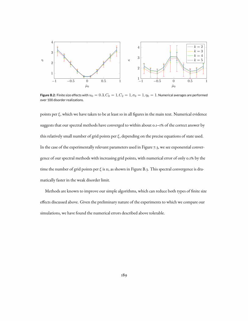
1 0.5 0 0.5 1

1

2

3

4

µ0

1 0.5 0 0.5 11

2

3

4

µ0

k = 2k = 3k = 4k = 5

Figure 1: testingFigure B.2: Finite size effects withu0 = 0.3,C0 = 1,C2 = 1,σ0 = 1, η0 = 1. Numerical averages are performed

over 100 disorder realizations.

points per ξ, which we have taken to be at least 10 in all figures in the main text. Numerical evidence

suggests that our spectral methods have converged to within about 0.1–1% of the correct answer by

this relatively small number of grid points per ξ, depending on the precise equations of state used.

In the case of the experimentally relevant parameters used in Figure 7.3, we see exponential conver-

gence of our spectral methods with increasing grid points, with numerical error of only 0.1% by the

time the number of grid points per ξ is 11, as shown in Figure B.3. This spectral convergence is dra-

matically faster in the weak disorder limit.

Methods are known to improve our simple algorithms, which can reduce both types of finite size

effects discussed above. Given the preliminary nature of the experiments to which we compare our

simulations, we have found the numerical errors described above tolerable.

189

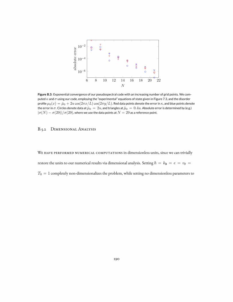
6 8 10 12 14 16 18 20 22

10

6

10

4

10

2

N

absoluteerror

Figure 1: testingFigure B.3: Exponential convergence of our pseudospectral codewith an increasing number of grid points. We com-

putedκ andσ using our code, employing the “experimental” equations of state given in Figure 7.3, and the disorder

profileµ0(x) = µ0 + 2u cos(2πx/L) cos(2πy/L). Red data points denote the error inκ, and blue points denotethe error inσ. Circles denote data at µ0 = 2u, and triangles at µ0 = 0.4u. Absolute error is determined by (e.g.)

|σ(N)− σ(29)|/σ(29), where we use the data points atN = 29 as a reference point.

B.5.2 Dimensional Analysis

We have performed numerical computations in dimensionless units, since we can trivially

restore the units to our numerical results via dimensional analysis. Setting ℏ = kB = e = vF =

T0 = 1 completely non-dimensionalizes the problem, while setting no dimensionless parameters to

190

unity. We can now trivially restore the units as follows:

L =ℏvFkBT0

× Lnumerics ∼ (100 nm)× Lnumerics (B.28a)

µ = kBT0 × µnumerics ∼ (5 meV)× µnumerics, (B.28b)

σ =e2

ℏ× σnumerics ∼ (0.25 k −1)× σnumerics, (B.28c)

α =kBe

ℏ× αnumerics ∼

(20

nWV

)× αnumerics, (B.28d)

κ =k2BT0

ℏ× κnumerics ∼

(0.1

nWK

)× κnumerics. (B.28e)

We have also noted the approximate scale of each important physical quantity in the problem for

convenience.

191

References

[1] Albert Einstein. Investigations on the Theory of the Brownian Movement. Courier Corpora-tion, 1956. ISBN 978-0-486-60304-9.

[2] R. Kubo. The fluctuation-dissipation theorem. Reports on Progress in Physics, 29(1):255, 1966.ISSN 0034-4885. doi: 10.1088/0034-4885/29/1/306. URL http://stacks.iop.org/0034-4885/29/i=1/a=306.

[3] Herbert B. Callen and Theodore A. Welton. Irreversibility and Generalized Noise. PhysicalReview, 83(1):34–40, July 1951. doi: 10.1103/PhysRev.83.34. URL http://link.aps.org/doi/10.1103/PhysRev.83.34.

[4] H. Nyquist. Thermal Agitation of Electric Charge in Conductors. Physical Review, 32(1):110–113, July 1928. doi: 10.1103/PhysRev.32.110. URL http://link.aps.org/doi/10.1103/PhysRev.32.110.

[5] John B Johnson. Thermal agitation of electricity in conductors. Nature, 119(2984):50–51,1927.

[6] J. B. Johnson. Thermal Agitation of Electricity in Conductors. Physical Review, 32(1):97–109,July 1928. doi: 10.1103/PhysRev.32.97. URL http://link.aps.org/doi/10.1103/PhysRev.32.97.

[7] R. H. Dicke. The Measurement of Thermal Radiation at Microwave Frequencies. Reviewof Scientific Instruments, 17(7):268–275, July 1946. ISSN 0034-6748. doi: 10.1063/1.1770483.URL http://aip.scitation.org/doi/abs/10.1063/1.1770483.

[8] R. J. Schoelkopf, P. J. Burke, A. A. Kozhevnikov, D. E. Prober, and M. J. Rooks. FrequencyDependence of Shot Noise in a Diffusive Mesoscopic Conductor. Physical Review Letters,78(17):3370–3373, April 1997. doi: 10.1103/PhysRevLett.78.3370. URL http://link.aps.org/doi/10.1103/PhysRevLett.78.3370.

[9] David M. Pozar. Microwave Engineering. Wiley, Hoboken, NJ, 4 edition edition, November2011. ISBN 978-0-470-63155-3.

192

[10] Jesse Crossno, Xiaomeng Liu, Thomas A. Ohki, Philip Kim, and Kin Chung Fong. Develop-ment of high frequency and wide bandwidth Johnson noise thermometry. Applied PhysicsLetters, 106(2):023121, January 2015. ISSN 0003-6951, 1077-3118. doi: 10.1063/1.4905926. URLhttp://arxiv.org/abs/1411.4596. arXiv: 1411.4596.

[11] S. O. Rice. Mathematical analysis of random noise. The Bell System Technical Journal, 23(3):282–332, July 1944. ISSN 0005-8580. doi: 10.1002/j.1538-7305.1944.tb00874.x.

[12] Paul Horowitz and Winfield Hill. The Art of Electronics. Cambridge University Press,Cambridge England ; New York, 2 edition edition, July 1989. ISBN 978-0-521-37095-0.

[13] D. R. White, R. Galleano, A. Actis, H. Brixy, M. De Groot, J. Dubbeldam, A. L. Reesink,F. Edler, H. Sakurai, R. L. Shepard, and J. C. Gallop. The status of Johnson noise thermom-etry. Metrologia, 33(4):325, 1996. ISSN 0026-1394. doi: 10.1088/0026-1394/33/4/6. URLhttp://stacks.iop.org/0026-1394/33/i=4/a=6.

[14] D. C. Glattli, P. Jacques, A. Kumar, P. Pari, and L. Saminadayar. A noise detection schemewith 10 mK noise temperature resolution for semiconductor single electron tunneling devices.Journal of Applied Physics, 81:7350–7356, June 1997. ISSN 0021-8979. doi: 10.1063/1.365332.URL http://adsabs.harvard.edu/abs/1997JAP....81.7350G.

[15] L. DiCarlo, Y. Zhang, D. T. McClure, C. M. Marcus, L. N. Pfeiffer, and K. W. West. Sys-tem for measuring auto-and cross correlation of current noise at low temperatures. Rev SciInstrum, 77(7):073906–073906–7, 2006.

[16] M. Henny, S. Oberholzer, C. Strunk, and C. Schönenberger. 1/3-shot-noise suppression indiffusive nanowires. Physical Review B, 59(4):2871, 1999.

[17] James J. Brophy, Max Epstein, and Samuel L. Webb. Correlator‐Amplifier for Very LowLevel Signals. Rev Sci Instrum, 36(12):1803–1806, 1965. doi: 10.1063/1.1719469.

[18] H.-H. Klein, G. Klempt, and L. Storm. Measurement of the Thermodynamic Temperatureof 4 He at Various Vapour Pressures by a Noise Thermometer. Metrologia, 15(3):143, 1979.ISSN 0026-1394. doi: 10.1088/0026-1394/15/3/005. URL http://stacks.iop.org/0026-1394/15/i=3/a=005.

[19] N. Sampietro, Gianfranco Accomando, Luca Fasoli, Giorgio Ferrari, and Emilio Gatti. Highsensitivity noise measurement with a correlation spectrum analyzer. Instrumentation andMeasurement, IEEE Transactions on, 49(4):820–822, 2000.

193

[20] Neil W. Ashcroft and N. David Mermin. Solid State Physics. Brooks Cole, New York, 1edition edition, January 1976. ISBN 978-0-03-083993-1.

[21] Christopher McKitterick, Daniel Prober, and Boris Karasik. Performance of graphene ther-mal photon detectors. J Appl Phys, 113(4):044512–044512–6, 2013.

[22] Christopher B. McKitterick, Daniel E. Prober, and Michael J. Rooks. Electron-phononcooling in large monolayer graphene devices. Physical Review B, 93(7):075410, February2016. doi: 10.1103/PhysRevB.93.075410. URL https://link.aps.org/doi/10.1103/PhysRevB.93.075410.

[23] R. Franz and G. Wiedemann. Ueber die Wärme-Leitungsfähigkeit der Metalle. Annalen derPhysik, 165(8):497–531, January 1853. ISSN 1521-3889. doi: 10.1002/andp.18531650802. URLhttp://onlinelibrary.wiley.com/doi/10.1002/andp.18531650802/abstract.

[24] L. Lorenz. Bestimmung der Wärmegrade in absolutem Maasse. Annalen der Physik, 223(11):429–452, January 1872. ISSN 1521-3889. doi: 10.1002/andp.18722231107. URL http://onlinelibrary.wiley.com/doi/10.1002/andp.18722231107/abstract.

[25] G. S. Kumar, G. Prasad, and R. O. Pohl. Experimental determinations of the Lorenz number.Journal of Materials Science, 28(16):4261–4272, August 1993. ISSN 0022-2461, 1573-4803.doi: 10.1007/BF01154931. URL https://link.springer.com/article/10.1007/BF01154931.

[26] A. Sommerfeld. Zur Elektronentheorie der Metalle. Naturwissenschaften, 15(41):825–832,October 1927. ISSN 0028-1042, 1432-1904. doi: 10.1007/BF01505083. URL https://link.springer.com/article/10.1007/BF01505083.

[27] Andrew H. Steinbach, John M. Martinis, and Michel H. Devoret. Observation of Hot-Electron Shot Noise in a Metallic Resistor. Physical Review Letters, 76(20):3806–3809, May1996. doi: 10.1103/PhysRevLett.76.3806. URL https://link.aps.org/doi/10.1103/PhysRevLett.76.3806.

[28] Ya M. Blanter and M. Buttiker. Shot Noise in Mesoscopic Conductors. Physics Reports, 336(1-2):1–166, September 2000. ISSN 03701573. doi: 10.1016/S0370-1573(99)00123-4. URLhttp://arxiv.org/abs/cond-mat/9910158. arXiv: cond-mat/9910158.

194

[29] M. J. M. de Jong and C. W. J. Beenakker. Semiclassical theory of shot noise in meso-scopic conductors. Physica A: Statistical Mechanics and its Applications, 230(1):219–248, August 1996. ISSN 0378-4371. doi: 10.1016/0378-4371(96)00068-4. URL http://www.sciencedirect.com/science/article/pii/0378437196000684.

[30] J. K. Viljas and T. T. Heikkilä. Electron-phonon heat transfer in monolayer and bilayergraphene. Physical Review B, 81(24):245404, June 2010. doi: 10.1103/PhysRevB.81.245404.URL http://link.aps.org/doi/10.1103/PhysRevB.81.245404.

[31] R. Bistritzer and A. H. MacDonald. Electronic Cooling in Graphene. Physical ReviewLetters, 102(20):206410, May 2009. doi: 10.1103/PhysRevLett.102.206410. URL http://link.aps.org/doi/10.1103/PhysRevLett.102.206410.

[32] Justin C. W. Song, Michael Y. Reizer, and Leonid S. Levitov. Disorder-Assisted Electron-Phonon Scattering and Cooling Pathways in Graphene. Physical Review Letters, 109(10):106602, September 2012. doi: 10.1103/PhysRevLett.109.106602. URL http://link.aps.org/doi/10.1103/PhysRevLett.109.106602.

[33] Wei Chen and Aashish A. Clerk. Electron-phonon mediated heat flow in disorderedgraphene. Physical Review B, 86(12):125443, September 2012. doi: 10.1103/PhysRevB.86.125443. URL http://link.aps.org/doi/10.1103/PhysRevB.86.125443.

[34] Thibault Sohier, Matteo Calandra, Cheol-Hwan Park, Nicola Bonini, Nicola Marzari, andFrancesco Mauri. Phonon-limited resistivity of graphene by first-principles calculations:Electron-phonon interactions, strain-induced gauge field, and Boltzmann equation. PhysicalReview B, 90(12):125414, September 2014. doi: 10.1103/PhysRevB.90.125414. URL https://link.aps.org/doi/10.1103/PhysRevB.90.125414.

[35] K. J. Tielrooij, N. C. H. Hesp, A. Principi, M. Lundeberg, E. A. A. Pogna, L. Banszerus,Z. Mics, M. Massicotte, P. Schmidt, D. Davydovskaya, K. Watanabe, T. Taniguchi, M. Bonn,D. Turchinovich, C. Stampfer, G. Cerullo, M. Polini, and F. H. L. Koppens. Out-of-planeheat transfer in van der Waals stacks: electron-hyperbolic phonon coupling. arXiv:1702.03766[cond-mat], February 2017. URL http://arxiv.org/abs/1702.03766. arXiv:1702.03766.

[36] Jürgen Schiefele, Fernando Sols, and Francisco Guinea. Temperature dependence of theconductivity of graphene on boron nitride. Physical Review B, 85(19):195420, May 2012. doi:

195

10.1103/PhysRevB.85.195420. URL https://link.aps.org/doi/10.1103/PhysRevB.85.195420.

[37] F. Bloch. Zum elektrischen Widerstandsgesetz bei tiefen Temperaturen. Zeitschrift fürPhysik, 59(3-4):208–214, March 1930. ISSN 0044-3328. doi: 10.1007/BF01341426. URLhttps://link.springer.com/article/10.1007/BF01341426.

[38] E. Grüneisen. Die Abhängigkeit des elektrischen Widerstandes reiner Metalle von derTemperatur. Annalen der Physik, 408(5):530–540, January 1933. ISSN 1521-3889. doi:10.1002/andp.19334080504. URL http://onlinelibrary.wiley.com/doi/10.1002/andp.19334080504/abstract.

[39] H. L. Stormer, L. N. Pfeiffer, K. W. Baldwin, and K. W. West. Observation of a Bloch-Gr\”uneisen regime in two-dimensional electron transport. Physical Review B, 41(2):1278–1281, January 1990. doi: 10.1103/PhysRevB.41.1278. URL https://link.aps.org/doi/10.1103/PhysRevB.41.1278.

[40] Dmitri K. Efetov and Philip Kim. Controlling Electron-Phonon Interactions in Grapheneat Ultrahigh Carrier Densities. Physical Review Letters, 105(25):256805, December 2010.doi: 10.1103/PhysRevLett.105.256805. URL https://link.aps.org/doi/10.1103/PhysRevLett.105.256805.

[41] Kin Chung Fong, Emma E. Wollman, Harish Ravi, Wei Chen, Aashish A. Clerk, M. D. Shaw,H. G. Leduc, and K. C. Schwab. Measurement of the Electronic Thermal ConductanceChannels and Heat Capacity of Graphene at Low Temperature. Physical Review X, 3(4):041008, October 2013. doi: 10.1103/PhysRevX.3.041008. URL http://link.aps.org/doi/10.1103/PhysRevX.3.041008.

[42] A. C. Betz, S. H. Jhang, E. Pallecchi, R. Ferreira, G. Fève, J.-M. Berroir, and B. Plaçais. Super-collision cooling in undoped graphene. Nature Physics, 9(2):109–112, February 2013. ISSN1745-2473. doi: 10.1038/nphys2494. URL http://www.nature.com/nphys/journal/v9/n2/abs/nphys2494.html.

[43] Matt W. Graham, Su-Fei Shi, Daniel C. Ralph, Jiwoong Park, and Paul L. McEuen. Pho-tocurrent measurements of supercollision cooling in graphene. Nature Physics, 9(2):103–108,February 2013. ISSN 1745-2473. doi: 10.1038/nphys2493. URL http://www.nature.com/nphys/journal/v9/n2/abs/nphys2493.html.

196

[44] S. S. Kubakaddi. Interaction of massless Dirac electrons with acoustic phonons in grapheneat low temperatures. Physical Review B, 79(7):075417, February 2009. doi: 10.1103/PhysRevB.79.075417. URL http://link.aps.org/doi/10.1103/PhysRevB.79.075417.

[45] Tony Low, Vasili Perebeinos, Raseong Kim, Marcus Freitag, and Phaedon Avouris. Coolingof photoexcited carriers in graphene by internal and substrate phonons. Physical Review B,86(4):045413, July 2012. doi: 10.1103/PhysRevB.86.045413. URL https://link.aps.org/doi/10.1103/PhysRevB.86.045413.

[46] D. R. Schmidt, R. J. Schoelkopf, and A. N. Cleland. Photon-Mediated Thermal Relax-ation of Electrons in Nanostructures. Physical Review Letters, 93(4):045901, July 2004.doi: 10.1103/PhysRevLett.93.045901. URL https://link.aps.org/doi/10.1103/PhysRevLett.93.045901.

[47] Christopher Burt McKitterick. Prospects for Ultra-sensitive Terahertz Photon Detectionwith Graphene. PhD thesis, Yale University, 2015. URL http://proberlab.yale.edu/sites/default/files/files/McKitterick_Thesis.pdf.

[48] Jae Hun Seol, Insun Jo, Arden L. Moore, Lucas Lindsay, Zachary H. Aitken, Michael T.Pettes, Xuesong Li, Zhen Yao, Rui Huang, David Broido, Natalio Mingo, Rodney S. Ruoff,and Li Shi. Two-Dimensional Phonon Transport in Supported Graphene. Science, 328(5975):213–216, April 2010. ISSN 0036-8075, 1095-9203. doi: 10.1126/science.1184014. URLhttp://science.sciencemag.org/content/328/5975/213.

[49] S. Yiğen and A. R. Champagne. Wiedemann–Franz Relation and Thermal-Transistor Effectin Suspended Graphene. Nano Letters, 14(1):289–293, January 2014. ISSN 1530-6984. doi:10.1021/nl403967z. URL http://dx.doi.org/10.1021/nl403967z.

[50] L. Wang, I. Meric, P. Y. Huang, Q. Gao, Y. Gao, H. Tran, T. Taniguchi, K. Watanabe, L. M.Campos, D. A. Muller, J. Guo, P. Kim, J. Hone, K. L. Shepard, and C. R. Dean. One-Dimensional Electrical Contact to a Two-Dimensional Material - Supplementary Materials.Science, 342(6158):614–617, November 2013. doi: 10.1126/science.1244358.

[51] Kin Chung Fong and K. C. Schwab. Ultrasensitive and Wide-Bandwidth Thermal Measure-ments of Graphene at Low Temperatures. Physical Review X, 2(3):031006, July 2012. doi:10.1103/PhysRevX.2.031006. URL http://link.aps.org/doi/10.1103/PhysRevX.2.031006.

197

[52] R. J. Schoelkopf, P. Wahlgren, A. A. Kozhevnikov, P. Delsing, and D. E. Prober. The radio-frequency single-electron transistor (RF-SET): A fast and ultrasensitive electrometer. Science,280(5367):1238–1242, January 1998.

[53] Jiamin Xue, Javier Sanchez-Yamagishi, Danny Bulmash, Philippe Jacquod, Aparna Desh-pande, K. Watanabe, T. Taniguchi, Pablo Jarillo-Herrero, and Brian J. LeRoy. Scanningtunnelling microscopy and spectroscopy of ultra-flat graphene on hexagonal boron nitride.Nature Materials, 10(4):282–285, April 2011. ISSN 1476-1122. doi: 10.1038/nmat2968. URLhttp://www.nature.com/nmat/journal/v10/n4/full/nmat2968.html.

[54] Shaffique Adam, Derek Ho, Indra Yudhistira, and Nilotpal Chakraborty. Theoretical studyof the criteria and consequences of hydrodynamic electron flow in graphene. In Bulletin ofthe American Physical Society, New Orleans, 2017. American Physical Society. URL http://meetings.aps.org/Meeting/MAR17/Session/X30.8.

[55] Jesse Crossno, Jing K. Shi, Ke Wang, Xiaomeng Liu, Achim Harzheim, Andrew Lucas, SubirSachdev, Philip Kim, Takashi Taniguchi, Kenji Watanabe, Thomas A. Ohki, and Kin ChungFong. Observation of the Dirac fluid and the breakdown of the Wiedemann-Franz law ingraphene. Science, 351(6277):1058–1061, March 2016. ISSN 0036-8075, 1095-9203. doi: 10.1126/science.aad0343. URL http://science.sciencemag.org/content/351/6277/1058.

[56] L. P. Kadanoff and P. C. Martin. Hydrodynamic equations and correlation functions. An-nals of Physics, 24:419–469, 1963.

[57] M. J. M. De Jong and L. W. Molenkamp. Hydrodynamic electron flow in high-mobilitywires. Physical Review B, 51(19):13389–13402, 1995.

[58] C. Cao, E. Elliott, J. Joseph, H. Wu, J. Petricka, T. Schäfer, and J. E. Thomas. UniversalQuantum Viscosity in a Unitary Fermi Gas. Science, 331(6013):58–61, January 2011. ISSN0036-8075, 1095-9203. doi: 10.1126/science.1195219. URL http://science.sciencemag.org/content/331/6013/58.

[59] E. Shuryak. Why does the quark-gluon plasma at RHIC behave as a nearly ideal fluid?Progress in Particle and Nuclear Physics, 53:273–303, 2004.

[60] Markus Müller and Subir Sachdev. Collective cyclotron motion of the relativistic plasma ingraphene. Physical Review B, 78(11), 2008.

198

[61] M. Foster and I. Aleiner. Slow imbalance relaxation and thermoelectric transport ingraphene. Physical Review B, 79(8):085415, 2009.

[62] S. S. Apostolov, A. Levchenko, and A. V. Andreev. Hydrodynamic Coulomb drag of stronglycorrelated electron liquids. Physical Review B, 89(12):121104, 2014.

[63] B. Narozhny, I. Gornyi, M. Titov, M. Schütt, and A. Mirlin. Hydrodynamics in graphene:Linear-response transport. Physical Review B, 91:035414, 2015.

[64] K. S. Novoselov, A. K. Geim, S. V. Morozov, D. Jiang, M. I. Katsnelson, I. V. Grigorieva, S. V.Dubonos, and A. A. Firsov. Two-dimensional gas of massless Dirac fermions in graphene.Nature, 438(7065):197–200, November 2005. ISSN 0028-0836. doi: 10.1038/nature04233.URL http://www.nature.com/nature/journal/v438/n7065/full/nature04233.html.

[65] Yuanbo Zhang, Yan-Wen Tan, Horst L. Stormer, and Philip Kim. Experimental obser-vation of the quantum Hall effect and Berry’s phase in graphene. Nature, 438(7065):201–204, November 2005. ISSN 0028-0836. doi: 10.1038/nature04235. URL http://www.nature.com/nature/journal/v438/n7065/full/nature04235.html.

[66] D. Siegel, W. Regan, A. Fedorov, A. Zettl, and A. Lanzara. Charge-Carrier Screening inSingle-Layer Graphene. Physical Review Letters, 110(14):146802, 2013.

[67] D. Sheehy and J. Schmalian. Quantum Critical Scaling in Graphene. Physical Review Letters,99(22):226803, 2007.

[68] B. Keimer and S. Sachdev. Quantum Criticality. Physics Today, 64:29, 2011.

[69] C. H. Lui, K. F. Mak, J. Shan, and T. F. Heinz. Ultrafast Photoluminescence from Graphene.Physical Review Letters, 105(12):127404, 2010.

[70] Markus Breusing, Claus Ropers, and Thomas Elsaesser. Ultrafast Carrier Dynamics inGraphite. Physical Review Letters, 102(8):086809, February 2009. doi: 10.1103/PhysRevLett.102.086809. URL https://link.aps.org/doi/10.1103/PhysRevLett.102.086809.

[71] K. J. Tielrooij, J. C. W. Song, S. A. Jensen, A. Centeno, A. Pesquera, A. Zurutuza Elorza,M. Bonn, L. S. Levitov, and F. H. L. Koppens. Photoexcitation cascade and multiple hot-carrier generation in graphene. Nature Physics, 9:248, 2013.

199

[72] Jens Christian Johannsen, Søren Ulstrup, Federico Cilento, Alberto Crepaldi, Michele Za-cchigna, Cephise Cacho, I. C. Edmond Turcu, Emma Springate, Felix Fromm, ChristianRaidel, Thomas Seyller, Fulvio Parmigiani, Marco Grioni, and Philip Hofmann. DirectView of Hot Carrier Dynamics in Graphene. Physical Review Letters, 111(2):027403, July 2013.doi: 10.1103/PhysRevLett.111.027403. URL https://link.aps.org/doi/10.1103/PhysRevLett.111.027403.

[73] M. Müller, J. Schmalian, and L. Fritz. Graphene: A Nearly Perfect Fluid. Physical ReviewLetters, 103(2):025301, July 2009.

[74] Markus Müller, Lars Fritz, and Subir Sachdev. Quantum-critical relativistic magnetotrans-port in graphene. Physical Review B, 78(11):115406, September 2008. doi: 10.1103/PhysRevB.78.115406. URL https://link.aps.org/doi/10.1103/PhysRevB.78.115406.

[75] Nicholas Wakeham, Alimamy F. Bangura, Xiaofeng Xu, Jean-Francois Mercure, MarthaGreenblatt, and Nigel E. Hussey. Gross violation of the Wiedemann–Franz law in a quasi-one-dimensional conductor. Nature Communications, 2:396, July 2011. ISSN 2041-1723.doi: 10.1038/ncomms1406. URL http://www.nature.com/ncomms/journal/v2/n7/full/ncomms1406.html.

[76] R. P. Smith, M. Sutherland, G. G. Lonzarich, S. S. Saxena, N. Kimura, S. Takashima, M. No-hara, and H. Takagi. Marginal breakdown of the Fermi-liquid state on the border of metallicferromagnetism. Nature, 455(7217):1220–1223, 2008.

[77] H. Pfau and et al. Thermal and electrical transport across a magnetic quantum critical point.Nature, 484(7395):493–497, 2012.

[78] R. W. Hill, C. Proust, L. Taillefer, P. Fournier, and R. L. Greene. Breakdown of Fermi-liquidtheory in a copper-oxide superconductor. Nature, 414(6865):711–715, 2001.

[79] Lars Fritz, Jörg Schmalian, Markus Müller, and Subir Sachdev. Quantum critical transport inclean graphene. Physical Review B, 78(8):085416, 2008.

[80] Shaffique Adam, E. H. Hwang, V. M. Galitski, and S. Das Sarma. A self-consistent theoryfor graphene transport. Proceedings of the National Academy of Sciences, 104(47):18392–18397, November 2007. ISSN 0027-8424, 1091-6490. doi: 10.1073/pnas.0704772104. URLhttp://www.pnas.org/content/104/47/18392.

200

[81] J. Martin, N. Akerman, G. Ulbricht, T. Lohmann, J. H. Smet, K. von Klitzing, and A. Yacoby.Observation of electron–hole puddles in graphene using a scanning single-electron transistor.Nature Physics, 4(2):144–148, February 2008. ISSN 1745-2473. doi: 10.1038/nphys781. URLhttp://www.nature.com/nphys/journal/v4/n2/abs/nphys781.html.

[82] Yuanbo Zhang, Victor W. Brar, Caglar Girit, Alex Zettl, and Michael F. Crommie. Ori-gin of spatial charge inhomogeneity in graphene. Nature Physics, 5(10):722–726, October2009. ISSN 1745-2473. doi: 10.1038/nphys1365. URL http://www.nature.com/nphys/journal/v5/n10/abs/nphys1365.html.

[83] C. R. Dean and et al. Boron nitride substrates for high-quality graphene electronics. NatureNanotechnology, 5(10):722–726, 2010.

[84] N. J. G. Couto, D. Costanzo, S. Engels, D.-K. Ki, K. Watanabe, T. Taniguchi, C. Stampfer,F. Guinea, and A. F. Morpurgo. Random Strain Fluctuations as Dominant Disorder Sourcefor High-Quality On-Substrate Graphene Devices. Physical Review X, 4(4):041019, 2014.

[85] AC Betz, F Vialla, D Brunel, C Voisin, M Picher, A Cavanna, A Madouri, G Fève, J-MBerroir, and B Plaçais. Hot electron cooling by acoustic phonons in graphene. PhysicalReview Letters, 109(5):56805, 2012.

[86] A. Laitinen, M. Oksanen, A. Fay, D. Cox, M. Tomi, P. Virtanen, and P. J. Hakonen.Electron-phonon coupling in suspended graphene: supercollisions by ripples. Nano Let-ters, 14:3009–3013, 2014.

[87] Sean A. Hartnoll, Pavel K. Kovtun, Markus Müller, and Subir Sachdev. Theory of theNernst effect near quantum phase transitions in condensed matter and in dyonic black holes.Physical Review B, 76(14):144502, October 2007. doi: 10.1103/PhysRevB.76.144502. URLhttps://link.aps.org/doi/10.1103/PhysRevB.76.144502.

[88] Andrew Lucas. Hydrodynamic transport in strongly coupled disordered quantum fieldtheories. New Journal of Physics, 17(11):113007, October 2015. ISSN 1367-2630. doi: 10.1088/1367-2630/17/11/113007. URL http://arxiv.org/abs/1506.02662. arXiv: 1506.02662.

[89] Andrew Lucas, Jesse Crossno, Kin Chung Fong, Philip Kim, and Subir Sachdev. Transport ininhomogeneous quantum critical fluids and in the Dirac fluid in graphene. Physical ReviewB, 93(7):075426, February 2016. doi: 10.1103/PhysRevB.93.075426. URL https://link.aps.org/doi/10.1103/PhysRevB.93.075426.

201

[90] P.  K. Kovtun, D. T. Son, and A. O. Starinets. Viscosity in Strongly Interacting QuantumField Theories from Black Hole Physics. Physical Review Letters, 94(11):111601, March 2005.doi: 10.1103/PhysRevLett.94.111601. URL https://link.aps.org/doi/10.1103/PhysRevLett.94.111601.

[91] Alessandro Principi, Giovanni Vignale, Matteo Carrega, and Marco Polini. Bulk and shearviscosities of the 2d electron liquid in a doped graphene sheet. arXiv.org, 2015. arXiv:1506.06030v1.

[92] G. S. Nolas and H. J. Goldsmid. Thermal Conductivity of Semiconductors. In Terry M.Tritt, editor, Thermal Conductivity, Physics of Solids and Liquids, pages 105–121. SpringerUS, 2004. ISBN 978-0-306-48327-1 978-0-387-26017-4. URL http://link.springer.com/chapter/10.1007/0-387-26017-X_4. DOI: 10.1007/0-387-26017-X_4.

[93] H. J. Goldsmid. The Thermal Conductivity of Bismuth Telluride. Proceedings of the PhysicalSociety. Section B, 69(2):203, 1956. ISSN 0370-1301. doi: 10.1088/0370-1301/69/2/310. URLhttp://stacks.iop.org/0370-1301/69/i=2/a=310.

[94] H. Yoshino and K. Murata. Significant enhancement of electronic thermal conductivity oftwo-dimensional zero-gap systems by bipolar-diffusion effect. Journal of the Physical Societyof Japan, 84(2):024601, January 2015. ISSN 0031-9015. doi: 10.7566/JPSJ.84.024601. URLhttp://journals.jps.jp/doi/abs/10.7566/JPSJ.84.024601.

[95] E. H. Hwang and S. Das Sarma. Screening-induced temperature-dependent transport in two-dimensional graphene. Physical Review B, 79(16):165404, April 2009. doi: 10.1103/PhysRevB.79.165404. URL https://link.aps.org/doi/10.1103/PhysRevB.79.165404.

[96] D. A. Bandurin, I. Torre, R. Krishna Kumar, M. Ben Shalom, A. Tomadin, A. Principi, G. H.Auton, E. Khestanova, K. S. Novoselov, I. V. Grigorieva, L. A. Ponomarenko, A. K. Geim,and M. Polini. Negative local resistance caused by viscous electron backflow in graphene.Science, 351(6277):1055–1058, March 2016. ISSN 0036-8075, 1095-9203. doi: 10.1126/science.aad0201. URL http://science.sciencemag.org/content/351/6277/1055.

[97] Philip J. W. Moll, Pallavi Kushwaha, Nabhanila Nandi, Burkhard Schmidt, and Andrew P.Mackenzie. Evidence for hydrodynamic electron flow in PdCoO2. Science, 351(6277):1061–1064, March 2016. ISSN 0036-8075, 1095-9203. doi: 10.1126/science.aac8385. URL http://science.sciencemag.org/content/351/6277/1061.

202

[98] Jan Zaanen. Electrons go with the flow in exotic material systems. Science, 351(6277):1026–1027, March 2016. ISSN 0036-8075, 1095-9203. doi: 10.1126/science.aaf2487. URL http://science.sciencemag.org/content/351/6277/1026.

[99] U. Briskot, M. Schütt, I. V. Gornyi, M. Titov, B. N. Narozhny, and A. D. Mirlin. Collision-dominated nonlinear hydrodynamics in graphene. Physical Review B, 92(11):115426, Septem-ber 2015. doi: 10.1103/PhysRevB.92.115426. URL https://link.aps.org/doi/10.1103/PhysRevB.92.115426.

[100] David Pines. Theory Of Quantum Liquids: Normal Fermi Liquids. Westview Press, Read-ing, Mass, March 1994. ISBN 978-0-201-40774-7.

[101] C. P. Weber, N. Gedik, J. E. Moore, J. Orenstein, J. Stephens, and D. D. Awschalom. Ob-servation of spin Coulomb drag in a two-dimensional electron gas. Nature, 437(7063):1330–1333, October 2005. ISSN 0028-0836. doi: 10.1038/nature04206. URL http://www.nature.com/nature/journal/v437/n7063/full/nature04206.html.

[102] Luyi Yang, J. D. Koralek, J. Orenstein, D. R. Tibbetts, J. L. Reno, and M. P. Lilly. Dopplervelocimetry of spin propagation in a two-dimensional electron gas. Nature Physics, 8(2):153–157, February 2012. ISSN 1745-2473. doi: 10.1038/nphys2157. URL http://www.nature.com/nphys/journal/v8/n2/abs/nphys2157.html.

[103] A. V. Andreev, Steven A. Kivelson, and B. Spivak. Hydrodynamic Description of Transportin Strongly Correlated Electron Systems. Physical Review Letters, 106(25):256804, June 2011.doi: 10.1103/PhysRevLett.106.256804. URL https://link.aps.org/doi/10.1103/PhysRevLett.106.256804.

[104] M. Mendoza, H. J. Herrmann, and S. Succi. Preturbulent Regimes in Graphene Flow. Phys-ical Review Letters, 106(15):156601, April 2011. doi: 10.1103/PhysRevLett.106.156601. URLhttps://link.aps.org/doi/10.1103/PhysRevLett.106.156601.

[105] Andrea Tomadin, Giovanni Vignale, and Marco Polini. Corbino Disk Viscometer for2d Quantum Electron Liquids. Physical Review Letters, 113(23):235901, December 2014.doi: 10.1103/PhysRevLett.113.235901. URL https://link.aps.org/doi/10.1103/PhysRevLett.113.235901.

[106] Alessandro Principi and Giovanni Vignale. Violation of the Wiedemann-Franz Law inHydrodynamic Electron Liquids. Physical Review Letters, 115(5):056603, July 2015. doi:

203

10.1103/PhysRevLett.115.056603. URL https://link.aps.org/doi/10.1103/PhysRevLett.115.056603.

[107] Iacopo Torre, Andrea Tomadin, Andre K. Geim, and Marco Polini. Nonlocal transport andthe hydrodynamic shear viscosity in graphene. Physical Review B, 92(16):165433, October2015. doi: 10.1103/PhysRevB.92.165433. URL https://link.aps.org/doi/10.1103/PhysRevB.92.165433.

[108] Leonid Levitov and Gregory Falkovich. Electron viscosity, current vortices and negativenonlocal resistance in graphene. Nature Physics, 12(7):672–676, July 2016. ISSN 1745-2473.doi: 10.1038/nphys3667. URL http://www.nature.com/nphys/journal/v12/n7/full/nphys3667.html.

[109] D. van der Marel, H. J. A. Molegraaf, J. Zaanen, Z. Nussinov, F. Carbone, A. Damascelli,H. Eisaki, M. Greven, P. H. Kes, and M. Li. Quantum critical behaviour in a high-Tcsuperconductor. Nature, 425(6955):271–274, September 2003. ISSN 0028-0836. doi:10.1038/nature01978. URL http://www.nature.com/nature/journal/v425/n6955/full/nature01978.html.

[110] R. A. Cooper, Y. Wang, B. Vignolle, O. J. Lipscombe, S. M. Hayden, Y. Tanabe, T. Adachi,Y. Koike, M. Nohara, H. Takagi, Cyril Proust, and N. E. Hussey. Anomalous Criticality inthe Electrical Resistivity of La2–xSrxCuO4. Science, 323(5914):603–607, January 2009. ISSN0036-8075, 1095-9203. doi: 10.1126/science.1165015. URL http://science.sciencemag.org/content/323/5914/603.

[111] Guohong Li, Adina Luican, and Eva Y. Andrei. Scanning Tunneling Spectroscopyof Graphene on Graphite. Physical Review Letters, 102(17):176804, April 2009. doi:10.1103/PhysRevLett.102.176804. URL https://link.aps.org/doi/10.1103/PhysRevLett.102.176804.

[112] Kedar Damle and Subir Sachdev. Nonzero-temperature transport near quantum criticalpoints. Physical Review B, 56(14):8714–8733, October 1997. doi: 10.1103/PhysRevB.56.8714.URL https://link.aps.org/doi/10.1103/PhysRevB.56.8714.

[113] Subir Sachdev. Quantum Phase Transitions. Cambridge University Press, Cambridge ; NewYork, 2 edition edition, May 2011. ISBN 978-0-521-51468-2.

204

[114] Richard A. Davison, Koenraad Schalm, and Jan Zaanen. Holographic duality and the resistiv-ity of strange metals. Physical Review B, 89(24):245116, June 2014. doi: 10.1103/PhysRevB.89.245116. URL https://link.aps.org/doi/10.1103/PhysRevB.89.245116.

[115] Mike Blake, David Tong, and David Vegh. Holographic Lattices Give the Graviton an Effec-tive Mass. Physical Review Letters, 112(7):071602, February 2014. doi: 10.1103/PhysRevLett.112.071602. URL https://link.aps.org/doi/10.1103/PhysRevLett.112.071602.

[116] Koushik Balasubramanian and Christopher P. Herzog. Losing forward momentum holo-graphically. Classical and Quantum Gravity, 31(12):125010, 2014. ISSN 0264-9381. doi:10.1088/0264-9381/31/12/125010. URL http://stacks.iop.org/0264-9381/31/i=12/a=125010.

[117] Andrew Lucas, Subir Sachdev, and Koenraad Schalm. Scale-invariant hyperscaling-violatingholographic theories and the resistivity of strange metals with random-field disorder. PhysicalReview D, 89(6):066018, March 2014. doi: 10.1103/PhysRevD.89.066018. URL https://link.aps.org/doi/10.1103/PhysRevD.89.066018.

[118] Andrew Lucas. Conductivity of a strange metal: from holography to memory func-tions. Journal of High Energy Physics, 2015(3):71, March 2015. ISSN 1029-8479. doi:10.1007/JHEP03(2015)071. URL https://link.springer.com/article/10.1007/JHEP03(2015)071.

[119] Richard A. Davison and Blaise Goutéraux. Dissecting holographic conductivities.Journal of High Energy Physics, 2015(9):90, September 2015. ISSN 1029-8479. doi:10.1007/JHEP09(2015)090. URL https://link.springer.com/article/10.1007/JHEP09(2015)090.

[120] Mike Blake. Momentum relaxation from the fluid/gravity correspondence. Journal of HighEnergy Physics, 2015(9):10, September 2015. ISSN 1029-8479. doi: 10.1007/JHEP09(2015)010.URL https://link.springer.com/article/10.1007/JHEP09(2015)010.

[121] Aristomenis Donos and Jerome P. Gauntlett. Navier-Stokes equations on black hole hori-zons and DC thermoelectric conductivity. Physical Review D, 92(12):121901, December2015. doi: 10.1103/PhysRevD.92.121901. URL https://link.aps.org/doi/10.1103/PhysRevD.92.121901.

205

[122] Sašo Grozdanov, Andrew Lucas, Subir Sachdev, and Koenraad Schalm. Absence of Disorder-Driven Metal-Insulator Transitions in Simple Holographic Models. Physical Review Letters,115(22):221601, November 2015. doi: 10.1103/PhysRevLett.115.221601. URL https://link.aps.org/doi/10.1103/PhysRevLett.115.221601.

[123] Enrico Rossi and S. Das Sarma. Ground State of Graphene in the Presence of RandomCharged Impurities. Physical Review Letters, 101(16):166803, October 2008. doi: 10.1103/PhysRevLett.101.166803. URL https://link.aps.org/doi/10.1103/PhysRevLett.101.166803.

[124] Enrico Rossi, S. Adam, and S. Das Sarma. Effective medium theory for disordered two-dimensional graphene. Physical Review B, 79(24):245423, June 2009. doi: 10.1103/PhysRevB.79.245423. URL https://link.aps.org/doi/10.1103/PhysRevB.79.245423.

[125] Dmitry K. Efimkin and Victor Galitski. Strongly interacting Dirac liquid on the surface ofa topological Kondo insulator. Physical Review B, 90(8):081113, August 2014. doi: 10.1103/PhysRevB.90.081113. URL https://link.aps.org/doi/10.1103/PhysRevB.90.081113.

[126] Ling Lu, Zhiyu Wang, Dexin Ye, Lixin Ran, Liang Fu, John D. Joannopoulos, and MarinSoljačić. Experimental observation of Weyl points. Science, 349(6248):622–624, August2015. ISSN 0036-8075, 1095-9203. doi: 10.1126/science.aaa9273. URL http://science.sciencemag.org/content/349/6248/622.

[127] Su-Yang Xu, Ilya Belopolski, Nasser Alidoust, Madhab Neupane, Guang Bian, ChenglongZhang, Raman Sankar, Guoqing Chang, Zhujun Yuan, Chi-Cheng Lee, Shin-Ming Huang,Hao Zheng, Jie Ma, Daniel S. Sanchez, BaoKai Wang, Arun Bansil, Fangcheng Chou, Pavel P.Shibayev, Hsin Lin, Shuang Jia, and M. Zahid Hasan. Discovery of a Weyl fermion semimetaland topological Fermi arcs. Science, 349(6248):613–617, August 2015. ISSN 0036-8075, 1095-9203. doi: 10.1126/science.aaa9297. URL http://science.sciencemag.org/content/349/6248/613.

[128] B. Q. Lv, H. M. Weng, B. B. Fu, X. P. Wang, H. Miao, J. Ma, P. Richard, X. C. Huang, L. X.Zhao, G. F. Chen, Z. Fang, X. Dai, T. Qian, and H. Ding. Experimental Discovery of WeylSemimetal TaAs. Physical Review X, 5(3):031013, July 2015. doi: 10.1103/PhysRevX.5.031013.URL https://link.aps.org/doi/10.1103/PhysRevX.5.031013.

206

[129] H. B. Nielsen and Masao Ninomiya. The Adler-Bell-Jackiw anomaly and Weyl fermions ina crystal. Physics Letters B, 130(6):389–396, November 1983. ISSN 0370-2693. doi: 10.1016/0370-2693(83)91529-0. URL http://www.sciencedirect.com/science/article/pii/0370269383915290.

[130] D. T. Son and B. Z. Spivak. Chiral anomaly and classical negative magnetoresistance of Weylmetals. Physical Review B, 88(10):104412, September 2013. doi: 10.1103/PhysRevB.88.104412.URL https://link.aps.org/doi/10.1103/PhysRevB.88.104412.

[131] Sean A. Hartnoll. Lectures on holographic methods for condensed matter physics. Classicaland Quantum Gravity, 26(22):224002, 2009. ISSN 0264-9381. doi: 10.1088/0264-9381/26/22/224002. URL http://stacks.iop.org/0264-9381/26/i=22/a=224002.

[132] Oskar Vafek. Anomalous Thermodynamics of Coulomb-Interacting Massless DiracFermions in Two Spatial Dimensions. Physical Review Letters, 98(21):216401, May 2007.doi: 10.1103/PhysRevLett.98.216401. URL https://link.aps.org/doi/10.1103/PhysRevLett.98.216401.

[133] Andrew Lucas and Subir Sachdev. Memory matrix theory of magnetotransport in strangemetals. Physical Review B, 91(19):195122, May 2015. doi: 10.1103/PhysRevB.91.195122. URLhttps://link.aps.org/doi/10.1103/PhysRevB.91.195122.

[134] Matthew Luzum and Paul Romatschke. Conformal relativistic viscous hydrodynamics:Applications to RHIC results at $\sqrts_\mathitnn=200$ GeV. Physical Review C,78(3):034915, September 2008. doi: 10.1103/PhysRevC.78.034915. URL https://link.aps.org/doi/10.1103/PhysRevC.78.034915.

[135] B. Huard, N. Stander, J. A. Sulpizio, and D. Goldhaber-Gordon. Evidence of the role ofcontacts on the observed electron-hole asymmetry in graphene. Physical Review B, 78(12):121402, September 2008. doi: 10.1103/PhysRevB.78.121402. URL https://link.aps.org/doi/10.1103/PhysRevB.78.121402.

[136] Scott Kirkpatrick. Classical Transport in Disordered Media: Scaling and Effective-MediumTheories. Physical Review Letters, 27(25):1722–1725, December 1971. doi: 10.1103/PhysRevLett.27.1722. URL https://link.aps.org/doi/10.1103/PhysRevLett.27.1722.

207

[137] B. Derrida and J. Vannimenus. A transfer-matrix approach to random resistor networks.Journal of Physics A: Mathematical and General, 15(10):L557, 1982. ISSN 0305-4470. doi:10.1088/0305-4470/15/10/007. URL http://stacks.iop.org/0305-4470/15/i=10/a=007.

[138] E. H. Hwang and S. Das Sarma. Acoustic phonon scattering limited carrier mobility intwo-dimensional extrinsic graphene. Physical Review B, 77(11):115449, March 2008. doi:10.1103/PhysRevB.77.115449. URL https://link.aps.org/doi/10.1103/PhysRevB.77.115449.

[139] K. I. Bolotin, K. J. Sikes, Z. Jiang, M. Klima, G. Fudenberg, J. Hone, P. Kim, and H. L.Stormer. Ultrahigh electron mobility in suspended graphene. Solid State Communica-tions, 146(9–10):351–355, June 2008. ISSN 0038-1098. doi: 10.1016/j.ssc.2008.02.024. URLhttp://www.sciencedirect.com/science/article/pii/S0038109808001178.

[140] Alexander S. Mayorov, Daniel C. Elias, Ivan S. Mukhin, Sergey V. Morozov, Leonid A.Ponomarenko, Kostya S. Novoselov, A. K. Geim, and Roman V. Gorbachev. HowClose Can One Approach the Dirac Point in Graphene Experimentally? Nano Letters,12(9):4629–4634, September 2012. ISSN 1530-6984. doi: 10.1021/nl301922d. URLhttp://dx.doi.org/10.1021/nl301922d.

[141] Jason Horng, Chi-Fan Chen, Baisong Geng, Caglar Girit, Yuanbo Zhang, Zhao Hao, Hans A.Bechtel, Michael Martin, Alex Zettl, Michael F. Crommie, Y. Ron Shen, and Feng Wang.Drude conductivity of Dirac fermions in graphene. Physical Review B, 83(16):165113, April2011. doi: 10.1103/PhysRevB.83.165113. URL https://link.aps.org/doi/10.1103/PhysRevB.83.165113.

[142] Fereshte Ghahari, Hong-Yi Xie, Takashi Taniguchi, Kenji Watanabe, Matthew S. Foster, andPhilip Kim. Enhanced Thermoelectric Power in Graphene: Violation of the Mott Relationby Inelastic Scattering. Physical Review Letters, 116(13):136802, March 2016. doi: 10.1103/PhysRevLett.116.136802. URL https://link.aps.org/doi/10.1103/PhysRevLett.116.136802.

[143] C. L. Kane and Matthew P. A. Fisher. Thermal Transport in a Luttinger Liquid. PhysicalReview Letters, 76(17):3192–3195, April 1996. doi: 10.1103/PhysRevLett.76.3192. URL https://link.aps.org/doi/10.1103/PhysRevLett.76.3192.

208

[144] S. Y. Li, Louis Taillefer, C. H. Wang, and X. H. Chen. Ballistic Magnon Transport andPhonon Scattering in the Antiferromagnet $\mathrmNd_2\mathrmCuO_4$.Physical Review Letters, 95(15):156603, October 2005. doi: 10.1103/PhysRevLett.95.156603.URL https://link.aps.org/doi/10.1103/PhysRevLett.95.156603.

[145] D. C. McCollum, R. L. Wild, and J. Callaway. Spin-Wave Thermal Conductivity of Ferro-magnetic EuS. Physical Review, 136(2A):A426–A428, October 1964. doi: 10.1103/PhysRev.136.A426. URL https://link.aps.org/doi/10.1103/PhysRev.136.A426.

[146] Aveek Bid, N. Ofek, H. Inoue, M. Heiblum, C. L. Kane, V. Umansky, and D. Mahalu.Observation of neutral modes in the fractional quantum Hall regime. Nature, 466(7306):585–590, July 2010. ISSN 0028-0836. doi: 10.1038/nature09277. URL http://www.nature.com/nature/journal/v466/n7306/full/nature09277.html.

[147] Hiroyuki Inoue, Anna Grivnin, Yuval Ronen, Moty Heiblum, Vladimir Umansky, and Di-ana Mahalu. Proliferation of neutral modes in fractional quantum Hall states. NatureCommunications, 5:4067, June 2014. ISSN 2041-1723. doi: 10.1038/ncomms5067. URL http://www.nature.com/ncomms/2014/140606/ncomms5067/full/ncomms5067.html.

[148] Vivek Venkatachalam, Sean Hart, Loren Pfeiffer, Ken West, and Amir Yacoby. Local ther-mometry of neutral modes on the quantum Hall edge. Nature Physics, 8(9):676–681,September 2012. ISSN 1745-2473. doi: 10.1038/nphys2384. URL http://www.nature.com/nphys/journal/v8/n9/full/nphys2384.html.

[149] A. Y. Kuntsevich, Y. V. Tupikov, V. M. Pudalov, and I. S. Burmistrov. Strongly correlatedtwo-dimensional plasma explored from entropy measurements. Nature Communications, 6:7298, June 2015. ISSN 2041-1723. doi: 10.1038/ncomms8298. URL http://www.nature.com/ncomms/2015/150623/ncomms8298/full/ncomms8298.html.

[150] P. Mazur and S. R. de Groot. On onsager’s relations in a magnetic field. Physica, 19(1):961–970, January 1953. ISSN 0031-8914. doi: 10.1016/S0031-8914(53)80108-4. URL http://www.sciencedirect.com/science/article/pii/S0031891453801084.

[151] L. Smrcka and P. Streda. Transport coefficients in strong magnetic fields. Journal of PhysicsC: Solid State Physics, 10(12):2153, 1977. ISSN 0022-3719. doi: 10.1088/0022-3719/10/12/021.URL http://stacks.iop.org/0022-3719/10/i=12/a=021.

209

[152] Yuri M. Zuev, Willy Chang, and Philip Kim. Thermoelectric and MagnetothermoelectricTransport Measurements of Graphene. Physical Review Letters, 102(9):096807, March 2009.doi: 10.1103/PhysRevLett.102.096807. URL https://link.aps.org/doi/10.1103/PhysRevLett.102.096807.

[153] Balázs Dóra and Peter Thalmeier. Magnetotransport and thermoelectricity in Landau-quantized disordered graphene. Physical Review B, 76(3):035402, July 2007. doi:10.1103/PhysRevB.76.035402. URL https://link.aps.org/doi/10.1103/PhysRevB.76.035402.

[154] Wen Long, Hui Zhang, and Qing-feng Sun. Quantum thermal Hall effect in graphene.Physical Review B, 84(7):075416, August 2011. doi: 10.1103/PhysRevB.84.075416. URLhttps://link.aps.org/doi/10.1103/PhysRevB.84.075416.

[155] V. P. Gusynin and S. G. Sharapov. Magnetic oscillations in planar systems with the Dirac-likespectrum of quasiparticle excitations. II. Transport properties. Physical Review B, 71(12):125124, March 2005. doi: 10.1103/PhysRevB.71.125124. URL https://link.aps.org/doi/10.1103/PhysRevB.71.125124.

[156] COMSOL Multiphysics®, 2017. URL www.comsol.com.

[157] Lloyd N. Trefethen. Spectral Methods in MATLAB. SIAM: Society for Industrial andApplied Mathematics, Philadelphia, PA, 62026th edition edition, February 2001. ISBN978-0-89871-465-4.

[158] Barry Smith, Petter Bjorstad, and William Gropp. Domain Decomposition: Parallel Mul-tilevel Methods for Elliptic Partial Differential Equations. Cambridge University Press,Cambridge, March 2004. ISBN 978-0-521-60286-0.

210

Kim group photo takenwhile hiking in theWhiteMountains (2015).

211