electronic theses and dissertations uc san diego
TRANSCRIPT

eScholarship provides open access, scholarly publishingservices to the University of California and delivers a dynamicresearch platform to scholars worldwide.
Electronic Theses and DissertationsUC San Diego
Peer Reviewed
Title:Data Reconstruction from a Hard Disk Drive using Magnetic Force Microscopy
Author:Kanekal, Vasu
Series:UC San Diego Electronic Theses and Dissertations
Degree:M.S.--University of California, San Diego--2013, UC San Diego
Permalink:https://escholarship.org/uc/item/26g4p84b
Local Identifier:b7825050
Abstract:The purpose of this study is to determine whether or not the data written on a modern high-densityhard disk drive can be recovered via magnetic force microscopy of the disks' surface. To this end,a variety of image processing techniques are utilized to process the raw images into a readilyusable form, and subsequently, a simulated read channel is designed to produce an estimate ofthe raw data corresponding to the magnetization pattern written on the disk. Using a speciallyprepared hard disk drive, the performance of this process is analyzed and techniques to improveit are investigated. Finally, some interesting results about maximal length shift register sequencesare presented
Copyright Information:All rights reserved unless otherwise indicated. Contact the author or original publisher for anynecessary permissions. eScholarship is not the copyright owner for deposited works. Learn moreat http://www.escholarship.org/help_copyright.html#reuse

UNIVERSITY OF CALIFORNIA, SAN DIEGO
Data Reconstruction from a Hard Disk Drive using Magnetic ForceMicroscopy
A Thesis submitted in partial satisfaction of the
requirements for the degree
Master of Science
in
Electrical Engineering (Signal and Image Processing)
by
Vasu Kanekal
Committee in charge:
Professor Paul H. Siegel, ChairProfessor Laurence B. MilsteinProfessor Truong Q. Nguyen
2013

Copyright
Vasu Kanekal, 2013
All rights reserved.

The Thesis of Vasu Kanekal is approved, and it is accept-
able in quality and form for publication on microfilm and
electronically:
Chair
University of California, San Diego
2013
iii

DEDICATION
To Mom, Dad, Lasya, and Vidya
iv

TABLE OF CONTENTS
Signature Page . . . . . . . . . . . . . . . . . . . . . . . . . . . . . . . . . . iii
Dedication . . . . . . . . . . . . . . . . . . . . . . . . . . . . . . . . . . . . . iv
Table of Contents . . . . . . . . . . . . . . . . . . . . . . . . . . . . . . . . . v
List of Figures . . . . . . . . . . . . . . . . . . . . . . . . . . . . . . . . . . vi
List of Tables . . . . . . . . . . . . . . . . . . . . . . . . . . . . . . . . . . . viii
Acknowledgements . . . . . . . . . . . . . . . . . . . . . . . . . . . . . . . . ix
Abstract of the Thesis . . . . . . . . . . . . . . . . . . . . . . . . . . . . . . x
Chapter 1 Introduction . . . . . . . . . . . . . . . . . . . . . . . . . . . . 1
Chapter 2 Literature Review and Research . . . . . . . . . . . . . . . . . 32.1 Data Recovery . . . . . . . . . . . . . . . . . . . . . . . . 32.2 Data Sanitization . . . . . . . . . . . . . . . . . . . . . . 8
Chapter 3 Background Information . . . . . . . . . . . . . . . . . . . . . 113.1 Digital Magnetic Recording Fundamentals . . . . . . . . 113.2 Magnetic Force Microscopy . . . . . . . . . . . . . . . . . 143.3 Hard Disk Drive Channels . . . . . . . . . . . . . . . . . 163.4 Digital Image Processing . . . . . . . . . . . . . . . . . . 243.5 Maximal Length Shift Register Sequences . . . . . . . . . 28
Chapter 4 MFM Based Data Reconstruction System . . . . . . . . . . . 314.1 System Overview and Experimental Setup . . . . . . . . 314.2 MFM Imaging and Image Processing . . . . . . . . . . . 334.3 PRML Channel . . . . . . . . . . . . . . . . . . . . . . . 404.4 Performance Analysis . . . . . . . . . . . . . . . . . . . . 46
Chapter 5 Extensions and Further Analysis . . . . . . . . . . . . . . . . . 515.1 Time-Frequency Analysis Methods . . . . . . . . . . . . . 515.2 Precoding of PN Sequences . . . . . . . . . . . . . . . . . 56
Chapter 6 Conclusion . . . . . . . . . . . . . . . . . . . . . . . . . . . . . 62
Bibliography . . . . . . . . . . . . . . . . . . . . . . . . . . . . . . . . . . . 63
v

LIST OF FIGURES
Figure 2.1: Guzik DTR 3000 Spin-stand . . . . . . . . . . . . . . . . . . . . 6Figure 2.2: Pits of a CD Imaged with a High-Power Microscope . . . . . . 8Figure 2.3: Garner TS1 Degausser . . . . . . . . . . . . . . . . . . . . . . . 10
Figure 3.1: A Modern Hard Disk Drive . . . . . . . . . . . . . . . . . . . . 12Figure 3.2: Longitudinal vs. Perpendicular Recording . . . . . . . . . . . . 13Figure 3.3: Block Diagram of Hard Disk Drive . . . . . . . . . . . . . . . . 14Figure 3.4: Dimension V SPM Head . . . . . . . . . . . . . . . . . . . . . . 15Figure 3.5: TappingMode Operation of SPM . . . . . . . . . . . . . . . . . 17Figure 3.6: Interleaved Scanning Method . . . . . . . . . . . . . . . . . . . 17Figure 3.7: Two-Pass LiftMode Scanning for MFM Imaging . . . . . . . . . 17Figure 3.8: Hard Disk Channel . . . . . . . . . . . . . . . . . . . . . . . . . 19Figure 3.9: Channel Impulse Response . . . . . . . . . . . . . . . . . . . . 20Figure 3.10: Receiver Block Diagram . . . . . . . . . . . . . . . . . . . . . . 20Figure 3.11: Partial Response Class I Target . . . . . . . . . . . . . . . . . . 21Figure 3.12: Trellis for PR1 Channel . . . . . . . . . . . . . . . . . . . . . . 23Figure 3.13: Digital Representation of Images . . . . . . . . . . . . . . . . . 25Figure 3.14: Pair of Images to be Stitched . . . . . . . . . . . . . . . . . . . 27Figure 3.15: Cross-Correlation Objective Function . . . . . . . . . . . . . . . 27Figure 3.16: Shift Register Implemented with D-Flip-Flops . . . . . . . . . . 30Figure 3.17: Linear Feedback Shift Register . . . . . . . . . . . . . . . . . . 30
Figure 4.1: System Block Diagram of MFM Based Data Recovery . . . . . 32Figure 4.2: Image Acquisition and Processing Stage . . . . . . . . . . . . . 34Figure 4.3: Raw MFM Images of Hard Disk Surface . . . . . . . . . . . . . 35Figure 4.4: Cross-Correlation Translational Motion Estimation . . . . . . . 36Figure 4.5: Heuristic Method to Segment Tracks . . . . . . . . . . . . . . . 38Figure 4.6: Statistical Texture Analysis Techniques . . . . . . . . . . . . . 39Figure 4.7: Procedure to Identify Guardbands using Texture Analysis and
Hough Transform . . . . . . . . . . . . . . . . . . . . . . . . . . 40Figure 4.8: PRML Channel to Detect Data from Processed MFM Images . 41Figure 4.9: Dipulse Response Estimated using Least-Squares Method . . . 43Figure 4.10: Comparison of Partial Response Targets to Dipulse Response . 44Figure 4.11: Required Partial Response Equalizer . . . . . . . . . . . . . . . 45Figure 4.12: Sampled and Equalized Readback Signal . . . . . . . . . . . . . 45Figure 4.13: Sixteen Stage Trellis for E2PR4 Channel . . . . . . . . . . . . . 46Figure 4.14: Comparison of Detected Sequence and Actual Sequence in One
Period . . . . . . . . . . . . . . . . . . . . . . . . . . . . . . . . 48Figure 4.15: Histogram of Observed Error Events in One Track . . . . . . . 49Figure 4.16: “Noise” Samples from Six Periods of One Track . . . . . . . . . 50
vi

Figure 5.1: Linear Chirp Signal and its Fourier Transform . . . . . . . . . . 53Figure 5.2: Linear Chirp Signal and its Spectrogram . . . . . . . . . . . . . 53Figure 5.3: Application of LEM Algorithm to Test Signal . . . . . . . . . . 55Figure 5.4: Chirping Degradation Model . . . . . . . . . . . . . . . . . . . 56Figure 5.5: Chirpiness Estimation using LEM on Synthetic Signal . . . . . 57Figure 5.6: Time-Frequency Distribution of Readback Signal . . . . . . . . 57
vii

LIST OF TABLES
Table 3.1: List of Common Partial Response Targets . . . . . . . . . . . . . 21
Table 4.1: 256-Bit Pattern Written onto Specially Formatted HDD . . . . . 33Table 4.2: Observed Symbol Error Rates from One Dataset . . . . . . . . . 48Table 4.3: Error Events for E2PR2 upto d2 = 280 . . . . . . . . . . . . . . 50
viii

ACKNOWLEDGEMENTS
First, I would like to acknowledge Prof. Paul H. Siegel, to whom I owe the
opportunity to perform this work, and without whose assistance would not have
been able to progress. Next, I would like to acknowledge Dr. Frederick E. Spada
who was responsible for acquiring all the magnetic force microscopy images used in
this work. Also, I would like to acknowledge Prof. Larry Milstein and Prof. Truong
Nguyen for agreeing to be on the committee. I have learned immensely through
the many courses I have taken with them. Finally, I would like to acknowledge the
United States Department of Defense, for funding these research efforts.
ix

ABSTRACT OF THE THESIS
Data Reconstruction from a Hard Disk Drive using Magnetic ForceMicroscopy
by
Vasu Kanekal
Master of Science in Electrical Engineering (Signal and Image Processing)
University of California, San Diego, 2013
Professor Paul H. Siegel, Chair
The purpose of this study is to determine whether or not the data writ-
ten on a modern high-density hard disk drive can be recovered via magnetic force
microscopy of the disks’ surface. To this end, a variety of image processing tech-
niques are utilized to process the raw images into a readily usable form, and sub-
sequently, a simulated read channel is designed to produce an estimate of the raw
data corresponding to the magnetization pattern written on the disk. Using a
specially prepared hard disk drive, the performance of this process is analyzed and
techniques to improve it are investigated. Finally, some interesting results about
maximal length shift register sequences are presented.
x
Chapter 1
Introduction
Hard disk drives are nowadays commonplace devices used to provide bulk
storage of the ever increasing amounts of data being produced every moment.
Magnetic force microscopy is one form of the class of modern microscopy called
scanning probe microscopy, which images the minute details of magnetic field in-
tensities on the surface of a sample. In this thesis, efforts to recover the data
written on a modern, high-density disk drive utilizing magnetic force microscopy
will be discussed.
The basic goal of this work is to answer the following questions. How could
one potentially recover the data written on a modern hard disk drive utilizing the
tool of magnetic force microscopy to image its surface and processing the result-
ing images? If there is a feasible method to do so, how accurately can this be
performed? If a disk containing confidential information is improperly sanitized
before disposal, could its contents be recovered through this procedure? To this
end, first the relationship between the images acquired through magnetic force mi-
croscopy and the signals involved in the read channel that is employed by the hard
disk drives themselves to read the data written on the disks must be determined.
Once this has been done, a system can be developed that takes advantage of this
relationship and uses the design principles involved in read channel engineering.
This was indeed the approach taken in this work, as will become clear through the
rest of the thesis.
The rest of this thesis is organized as follows. Chapter 2 reviews the prior
1

2
work done in the two main areas related to this project–data recovery and data
sanitization. Chapter 3 provides the necessary background in the subjects of mag-
netic recording, magnetic force microscopy, read channels, digital image processing,
and maximal length shift register sequences to explain the design and experimental
procedures performed in this work. Chapter 4 discusses the design, development,
and performance of a system that was used to experiment with recovering data
through magnetic force microscopy. Chapter 5 discusses some potential analy-
sis techniques to improve the performance of this system, and presents a result
regarding the invariance of maximal length sequences under precoding.

Chapter 2
Literature Review and Research
In looking at previous work of this nature, there are mainly two areas
that are of interest–data recovery and data sanitization. These have contradictory
goals, but progress in each is driven by progress in the other; effective sanitization
tries to eliminate the possibility of data recovery of sensitive information, while
effective recovery tries to get back data which might have been unintentionally or
intentionally lost (e.g. through improper sanitization). The rest of this chapter
will review the prior work that has been done in each of these areas.
2.1 Data Recovery
Providing the service of recovery of data from hard disk drives that are
unable to be read in a normal fashion composes a significant industry in which
many companies are involved. Generally, these services fall into two camps–those
for personal data recovery (like that which a graduate student might consult when
he finds his computer stops recognizing the hard drive on which resides the final
draft of his thesis), and those for forensic data recovery, where the goal is to recover
legal evidence which might have been intentionally deleted by the perpetrator.
Personal recovery services exist because hard drives, like any other complex system,
have some probability of failing due to one reason or another, and when there are
millions of drives being used in a variety of conditions, some inevitably fail. A
Bing search for “Data Recovery Services” in San Diego yields dozens of local
3

4
outfits willing to provide some sort of recovery service. The modes of failure
(or intentional destruction) are varied, and can allow recovery with as simple a
procedure as swapping its printed circuit board (PCB) with that of another drive
of a similar model, or render any form of recovery completely intractable. This
section will discuss some of the traditional hardware replacement based approaches
to data recovery as well as drive-independent methods. Furthermore, it will review
the work done on spin-stand based data recovery at the University of Maryland,
College Park and its relationship to the magnetic force microscopy (MFM) based
recovery in this work. Finally, it will discuss similar work done with optical media
using optical microscopy to reconstruct data via microscope imaging.
As discussed in [Sob04], the most common and successful methods of data
recovery from a failed drive are to replace selected hardware from the drive that
has failed with the same part from a drive of the same model. Note that all of
these methods assume that the data recorded on the magnetic surfaces of the
disks is completely intact. Examples include replacing the PCB, re-flashing the
firmware, replacing the headstack, and moving the disks to another drive. The
latter two need to be performed in a clean-room environment, since it is required
that the disks be free of even microscopic particles, since the flying heights of
the heads are usually on the order of nanometers! As the bit density of hard
disk drives is continually increasing, each drive is “hyper-tuned” at the factory,
where a myriad of parameters are optimized for the particular head and media
characteristics of each individual drive. This decreases the effectiveness of part
replacement techniques when a particular drive fails, as these optimized parameters
might vary significantly even among drives of the same model and batch. As a joint
effort between ActionFront Data Recovery Labs, Inc. and ChannelScience, a drive
independent method to allow recovery after replacing the headstack or transferring
disks to another drive was developed and presented at the 2004 IEEE NASA Mass
Storage Systems and Technologies Conference and published in [SOS06]. This
method developed custom hardware to replace the PCB of a drive, which then
performs the usual servo and channel functions that are controlled by custom
software. In order to allow the reconstruction of user data, the de-scrambling,

5
run-length limited (RLL) decoding, and error correction decoding (ECC) specifics
of a particular drive were reverse-engineered and implemented in software. Such a
method is an important contribution to the data recovery industry as it provides
a commercially viable technique to recover data from a drive when conventional
methods fail due to variations in the channel parameters of even drives of the same
model. This type of method can also cope with future density increases, provided
the newer channel codes and scrambling can be reverse-engineered as well. In sum,
the standard data recovery approaches assume that specific parts of a drive have
failed and that these can be replaced with those from a similar model. If these
still do not allow the drive to work normally, some custom hardware and software
can be developed to access the drive data in a lower level manner, providing some
drive-independence.
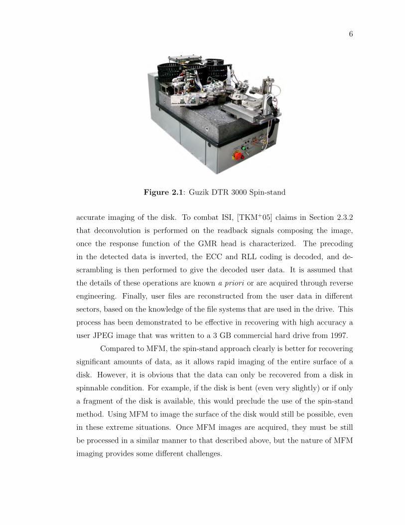
A more general approach to hard drive data recovery involves using a spin-
stand as pictured in Figure 2.1. On this device, the individual disks of the platter
are mounted, a giant magnetoresistive head (GMR) is flown above the surface,
and the response signal is captured. A series of papers from the lab of Prof.
Isaak Mayergoyz at the University of Maryland develop this technique, which is
based on utilizing the spin-stand as a type of magnetic force microscope, specific
to observing the magnetization patterns on a disk which can be spun. This allows
rapid imaging of large portions of the disk’s surface, and the resulting images have
to then be processed to recover the data written on the disk. One particular paper,
[TKM+05], describes the entire process. Specifically, the readback signal produced
by the GMR head as the disk is spun and the head is moved across the diameter
of the disk is composed into a contiguous rectangular image, covering the entire
drive. This is then processed to remove intersymbol interference (ISI), and from
this the data corresponding to the actual magnetization pattern is detected, and
further processed to ultimately yield user data. Some of the main challenges of
this approach are encountered first in the data acquisition stage, where the absence
of perfect centering of the disk on the spin-stand yields a sinusoidal distortion
of the tracks when imaged. This can be combated using proper centering, or
track following, where the head position is continuously adjusted to permit the
6
Figure 2.1: Guzik DTR 3000 Spin-stand
accurate imaging of the disk. To combat ISI, [TKM+05] claims in Section 2.3.2
that deconvolution is performed on the readback signals composing the image,
once the response function of the GMR head is characterized. The precoding
in the detected data is inverted, the ECC and RLL coding is decoded, and de-
scrambling is then performed to give the decoded user data. It is assumed that
the details of these operations are known a priori or are acquired through reverse
engineering. Finally, user files are reconstructed from the user data in different
sectors, based on the knowledge of the file systems that are used in the drive. This
process has been demonstrated to be effective in recovering with high accuracy a
user JPEG image that was written to a 3 GB commercial hard drive from 1997.
Compared to MFM, the spin-stand approach clearly is better for recovering
significant amounts of data, as it allows rapid imaging of the entire surface of a
disk. However, it is obvious that the data can only be recovered from a disk in
spinnable condition. For example, if the disk is bent (even very slightly) or if only
a fragment of the disk is available, this would preclude the use of the spin-stand
method. Using MFM to image the surface of the disk would still be possible, even
in these extreme situations. Once MFM images are acquired, they must be still
be processed in a similar manner to that described above, but the nature of MFM
imaging provides some different challenges.
7
Another set of work in Prof. Tom Milster’s group at the University of
Arizona has focused on data reconstruction from compact disks (CDs), based on
optical microscopy. In [KMFC04], a method is developed to utilize a high-power
optical microscope to acquire a set of images from the disk, perform image pro-
cessing to acquire a derived electronic signal, and from this the user data bytes are
retrieved using signal processing techniques. Specifically, an optical microscope is
focused onto a portion of the CD and the pattern of pits is digitally imaged. Each
image is subsequently preprocessed to correct for any rotation, and a threshold-
ing procedure employing Otsu’s method, a technique to automatically determine
the optimal threshold, is used to produce a binary image that distinguishes be-
tween the pits and lands. The tracks are separated by integrating the image in
the downtrack direction and finding the peaks, which correspond to the centers of
the tracks. From here, a signal similar to the electronic signal from a CD optical
reader system is derived. An automated system to capture images separated by
appropriate amounts is used to acquire several contiguous image frames and these
are stitched together based on the derived electronic signals from each. Once the
continuous electronic signals are derived from each track, they are then processed
to recover the user data. First, the RLL coding that is used in CDs (eight-to-
fourteen modulation) has to be decoded, and subsequently the cross-interleaved
Reed-Solomon coding has to be decoded to produce the user data. This method
has been shown to be effective in recovering small amounts of data in a reasonable
amount of time. One advantage in recovering data from CDs is that their coding
parameters are standardized in the rainbow books, which are a series of technical
specifications for various optical media maintained by independent organizations.
This is unlike the case for hard disk drives, where these coding parameters are
proprietary and would need to be reverse-engineered to successfully recover user
data. Another advantage is that ISI in the channel is not an issue, as can be seen
by the sharp images of the pits of a CD in Figure 2.2. Nonetheless, the overall
procedure developed in the present work using MFM imaging of hard disks is quite
similar to that described in [KMFC04].

8
Figure 2.2: Pits of a CD Imaged with a High-Power Microscope
2.2 Data Sanitization
At the other end of the spectrum is data sanitization, where the goal is
to prevent the recovery of confidential information stored on a hard drive by any
means. This is of primary importance to government agencies, but also to private
companies that are responsible for keeping their customers confidential information
secure. As discussed in [GS03], it should be of significant concern to personal users
as well, since when a user decides to replace a hard drive, not properly sanitizing it
could result in personal information, for example medical or financial records, being
stolen. Before a hard drive containing sensitive information is disposed of, it is
necessary to clear this information to prevent others from acquiring it. Performing
simple operating system level file deletion does not actually remove the data from
the drive, but instead merely deletes the pointers to the files from the file system.
This allows the retrieval of these “deleted” files with relative ease through the
operating system itself with a variety of available software. A more effective level
of cleansing is to actually overwrite the portions of the disk that contained the
user’s files, once or perhaps multiple times. Yet more effective is to use a degausser,
which employs strong magnetic fields to randomize the magnetization of the grains
on the magnetic medium of each disk. Most effective is physical destruction of the
hard drive, for example by disintegrating, pulverizing or melting. Generally, the
more effective the sanitization method, the more costly in both time and money

9
it is. Hence, in some situations, it is desired to utilize the least expensive method
that guarantees that recovery is infeasible. This section will discuss in a bit more
detail some of the sanitization methods and their effectiveness.
As mentioned, since operating system “delete” commands only remove file
header information from the file system as opposed to erasing the data from the
disk, manually overwriting is a more effective sanitization procedure. The details
of what pattern to overwrite with, and how many times, is somewhat a contentious
topic. Various procedures are (or were) described by various organizations and in-
dividuals, ranging from overwriting once with all zeros, to overwriting 35 times
with several rounds of random data followed by a slew of specific patterns. More
important is the fact that several blocks on the drive might not be logically acces-
sible through the operating system interface if they have been flagged as defective
after the drive has been in use for some time. In modern disk drives, this process
of removing tracks from the logical address space that have been deemed defective,
known as defect mapping, is continuously performed while tine drive is in operation.
To resolve this issue, an addition to the advanced technology attachment (ATA)
protocol called Secure Erase was developed by researchers at CMRR. This protocol
overwrites every possible user data record, including those that might have been
mapped out after the drive was used for some period [HCC09]. While overwriting
is significantly more secure than just deleting, it is still theoretically possible to
recover original data using microscopy or spin-stand techniques. One reason for
this is that when tracks are overwritten, it is unlikely that the head will traverse
the exact same path that it did the previous time the data was written, and hence
some of the original data could be left behind in the guardbands between tracks.
However, with modern high density drives, the guardbands are usually very small
compared to the tracks (or non-existent in the case of shingled magnetic recording)
making this ever more difficult. Finally, it should be noted that the drive is left in
usable condition with the overwriting method.
The next level of sanitization is degaussing, which utilizes an apparatus
known as a degausser, an example of which is pictured in Figure 2.3, to randomize
the polarity of magnetic grains on the magnetic media of the hard drive. There are

10
Figure 2.3: Garner TS1 Degausser
three main types of degaussers: coil, capacitive, and permanent magnet. The first
two utilize electromagnets to produce either a continuously strong, rapidly varying
magnetic field or an instantaneous but extremely strong magnetic field pulse to
randomly set the magnetization of individual domains in a hard drive’s media.
The last utilizes a permanent magnet that can produce a very strong magnetic
field, depending on the size of the magnet, but produces a constant field, that is
not time-varying. Depending on the coercivity of the magnetic medium used in
the drive, different levels of magnetic fields may be necessary to fully degauss a
drive. If an insufficient field strength is used, some remanant magnetic field may
be present on the disks, which can be observed using MFM for example. One of
the ultimate goals of this work is to determine whether the magnetization patterns
still visible via MFM after insufficient degaussing can be used to recover any data.
One important difference between degaussing and overwriting is that the drive
is rendered unusable after degaussing, since all servo regions are also erased. In
fact, if the fields used in degaussing are strong enough, the permanent magnets
in the drive’s motors might be demagnetized, clearly destroying the drive. The
most effective sanitization method is of course physical destruction, but degaussing
comes close, and often is performed before additional physical destruction for drives
containing highly confidential information.
Chapter 3
Background Information
3.1 Digital Magnetic Recording Fundamentals
Hard disk drives (HDDs) have had a remarkable history of growth and
development, starting with the IBM 350 disk storage unit in 1956, which had a
capacity of 3.75MB and weighed over a ton, to the latest 4TB 3.5 inch form factor
drive as of 2011. Clearly, the technology underlying hard drives has changed
dramatically in this time frame, and is expected to continue on this path. Despite
all the change, the basic concept of storing data as a magnetization pattern on
a physical medium which can be retrieved later by using a device that responds
as it flies over the pattern is still the principal idea used today. This section will
review the basic principles of operation of HDDs and furthermore the system level
abstraction.
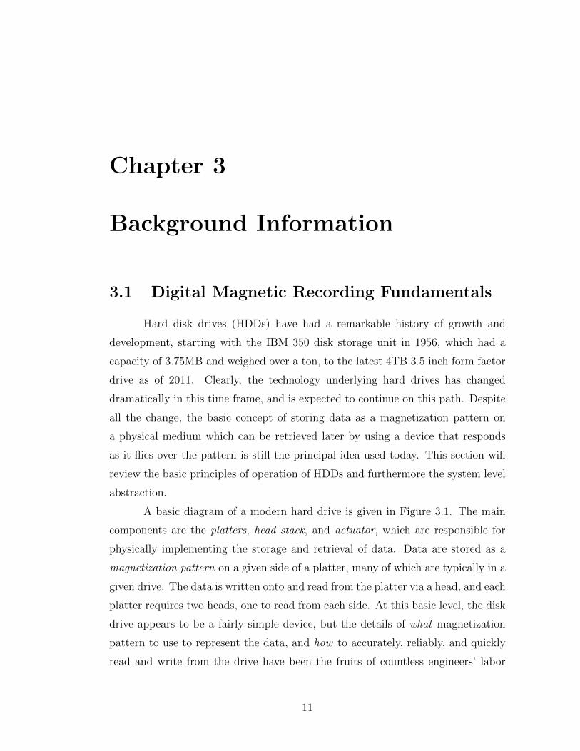
A basic diagram of a modern hard drive is given in Figure 3.1. The main
components are the platters, head stack, and actuator, which are responsible for
physically implementing the storage and retrieval of data. Data are stored as a
magnetization pattern on a given side of a platter, many of which are typically in a
given drive. The data is written onto and read from the platter via a head, and each
platter requires two heads, one to read from each side. At this basic level, the disk
drive appears to be a fairly simple device, but the details of what magnetization
pattern to use to represent the data, and how to accurately, reliably, and quickly
read and write from the drive have been the fruits of countless engineers’ labor
11

12
Figure 3.1: A Modern Hard Disk Drive
over the past couple of decades.
Early hard drives used a method called longitudinal recording, where a se-
quence of bits is represented by magnetizing a set of grains in one direction or
the other, parallel to the recording surface. By 2005, to allow the continuing push
for increasing recording density, a method called perpendicular recording began
to be used in commercially available drives. As the name suggests, the data is
represented by sets of grains magnetized perpendicular to the recording surface.
To allow this form of recording, the recording surface itself has to be designed
with a soft under layer that permits a monopole writing element to magnetize the
grains in the top layer in the desired manner. See Figure 3.2 for a comparison
between these two recording techniques. As the push for density is still increas-
ing, newer technologies are being considered, such as shingled magnetic recording
(SMR) and bit patterned recording (BPMR), which both take different approaches
to representing data using higher density magnetization patterns.
Once data are written to the drive, the retrieval of the data requires sensing
the magnetic pattern written on the drive, and the read head is responsible for the
preliminary task of transducing the magnetization pattern into an electrical signal
which can be further processed to recover the written data. Along with the changes
in recording methods, the read heads necessarily underwent technological changes
as well, from traditional ferrite wire-coil heads to the newer magneto-resistive
(MR), giant magneto-resistive (GMR), and tunneling magneto-resistive (TMR)

13
Figure 3.2: Longitudinal vs. Perpendicular Recording
heads. All of these, when paired with additional circuitry, produce a voltage signal
in response to flying over the magnetization pattern written on the disk, called
the readback or playback signal. It is this signal that contains the user data, but
in a highly encoded, distorted, and noisy form, and from which the rest of the
system must ultimately estimate the recorded data, hopefully with an extremely
low chance of making an error.
At the system level abstraction, the hard disk drive, or any storage de-
vice for that matter, can be interpreted as a digital communication system, and
in particular one that communicates messages from one point in time to another
(unfortunately, only forwards), rather than from one point in space to another.
Specifically, the preprocessor of user data which includes several layers of encoders
and the write head which transduces this encoded data into a magnetization pat-
tern on the platter compose the transmitter. The response of the read head to
the magnetization pattern and the thermal noise resulting from the electronics are
modeled as the channel. Finally, the receiver is composed of the blocks necessary
to first detect the encoded data, and then to decode this data to return the user
data. This level of abstraction makes readily available the theories of communica-
tion systems, information, and coding for the design of disk drive systems, and has
played a key role in allowing the ever increasing densities while still ensuring the
user data is preserved as accurately as possible. See Figure 3.3 for a block diagram
of HDD systems.

14
Figure 3.3: Block Diagram of Hard Disk Drive
3.2 Magnetic Force Microscopy
Modern microscopy has three main branches: optical or light, electron, and
scanning probe. Optical microscopes have the longest history and they operate by
passing visible light through or reflecting light from a sample, and passing this light
through a system of lenses which provide a magnified view due to the principles of
optics. Light microscopes allow direct visualization of the magnified specimen, but
ultimately have their resolution limited by the diffraction of light to the tenths of
microns. Electron microscopes, on the other hand, are one form of sub-diffraction
microscopy that utilize an electron beam with a much smaller wavelength than that
of visible light, thereby allowing even atomic level resolution. Yet another form
of sub-diffraction microscopy is scanning probe microscopy (SPM), which involves
scanning a physical probe across the surface of the specimen and measuring the
interactions between the probe and the sample. Magnetic force microscopy (MFM)
is one example of SPM, where a probe that is sensitive to magnetic fields is used.
This section will discuss some more details of SPM, and specifically the operation
of the Veeco Dimension V SPM in MFM mode as was used in this work.
Scanning probe microscopy utilizes a physical probe that interacts with
the surface of the sample as it is scanned, and it is this interaction which is in
turn measured while moving the probe in a raster scan. This results in a two-
dimensional grid of data, which can be visualized on a computer as a gray-scale
or false color image. The choice of the probe determines which features of the
15
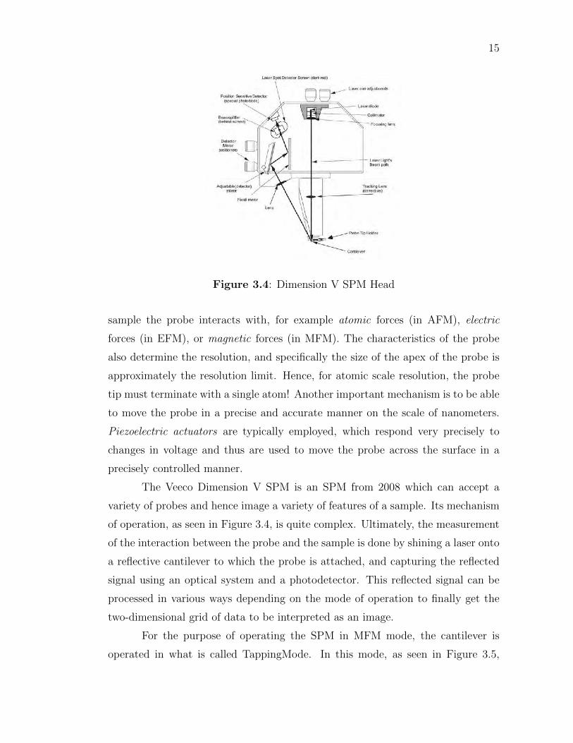
Figure 3.4: Dimension V SPM Head
sample the probe interacts with, for example atomic forces (in AFM), electric
forces (in EFM), or magnetic forces (in MFM). The characteristics of the probe
also determine the resolution, and specifically the size of the apex of the probe is
approximately the resolution limit. Hence, for atomic scale resolution, the probe
tip must terminate with a single atom! Another important mechanism is to be able
to move the probe in a precise and accurate manner on the scale of nanometers.
Piezoelectric actuators are typically employed, which respond very precisely to
changes in voltage and thus are used to move the probe across the surface in a
precisely controlled manner.
The Veeco Dimension V SPM is an SPM from 2008 which can accept a
variety of probes and hence image a variety of features of a sample. Its mechanism
of operation, as seen in Figure 3.4, is quite complex. Ultimately, the measurement
of the interaction between the probe and the sample is done by shining a laser onto
a reflective cantilever to which the probe is attached, and capturing the reflected
signal using an optical system and a photodetector. This reflected signal can be
processed in various ways depending on the mode of operation to finally get the
two-dimensional grid of data to be interpreted as an image.
For the purpose of operating the SPM in MFM mode, the cantilever is
operated in what is called TappingMode. In this mode, as seen in Figure 3.5,

16
the piezoelectric stack excites the cantilever with a vertical vibration, and the
cantilever responds in a manner depending on its resonant frequency, which is de-
tected by the reflected laser signal. For MFM imaging, scanning each line is a
two-step process, called an Interleave Scan, detailed in Figure 3.6. For each scan
line, the surface topography is first captured, which provides a profile of the sur-
face of the sample. Then, having learned this surface topography, the cantilever
ascends to a specific height, and follows the surface profile while rescanning the
line–it is during this scan that the MFM image is captured, as displayed in Figure
3.7. This allows the tip to respond to the stray magnetic field above the surface
of the sample while minimizing its response to other interactions that occur when
closer to the surface. Specifically, the magnetic force gradients from the surface of
the sample alter the resonant frequency of the cantilever, which can be detected
in one of three ways. This first is phase detection, where the phase shift between
the cantilever’s oscillation and the piezoelectric drive is measured. The second is
amplitude detection, which tracks changes in the amplitude of cantilever oscilla-
tion. The last is frequency modulation, where the drive frequency is modulated by
a feedback loop to maintain a 90 degree phase lag between the piezoelectric drive
and the cantilever oscillation, corresponding to resonance. In this work, all images
were acquired using phase detection.
3.3 Hard Disk Drive Channels
As mentioned in Section 3.1, the system level abstraction of a hard disk
drive as a digital communication system lends itself to useful analysis which al-
lows better designs. Along with the technology changes in the recording heads
and media, the channel designs necessarily had to improve to take advantage of
these. Specifically, early disk drives used peak detection read channels, which
were based on the fact that as a read head flies over a transition in magnetiza-
tion in longitudinal media, a current pulse is produced, and detecting the peaks
of these allows determining whether or not a transition was present. However,
as density continued to increase, the pulses would get closer and closer, causing

17
Figure 3.5: TappingMode Operation of SPM
Figure 3.6: Interleaved Scanning Method
Figure 3.7: Two-Pass LiftMode Scanning for MFM Imaging
18
pulse crowding (intersymbol interference (ISI) in the language of communication
systems), which rendered these channels unable to accurately read the magnetiza-
tion pattern. Thus was the introduction of partial response, maximum likelihood
(PRML) channels, which provided a sophisticated way to take advantage of the
ISI by controlling it to specific amounts in adjacent symbols. A maximum likeli-
hood receiver is in general very computationally complex, but the introduction of
the Viterbi algorithm provided an iterative approach that can be implemented in
real time. Of course, as the push of ever increasing density continues, the basic
PRML channel has been extended in several ways, e.g. using an adaptive target
and adaptive equalization. Furthermore, the coding schemes used in the channel
have also evolved over time, from early run-length limited or modulation codes, and
later Reed-Solomon codes, to the latest low density parity-check (LDPC) codes.
Also, with the research being done on newer heads and media, newer channels are
being investigated to take advantage of these, e.g. two dimensional channels for
two dimensional magnetic recording. The remainder of this section will discuss in
more detail the basic PRML channel.
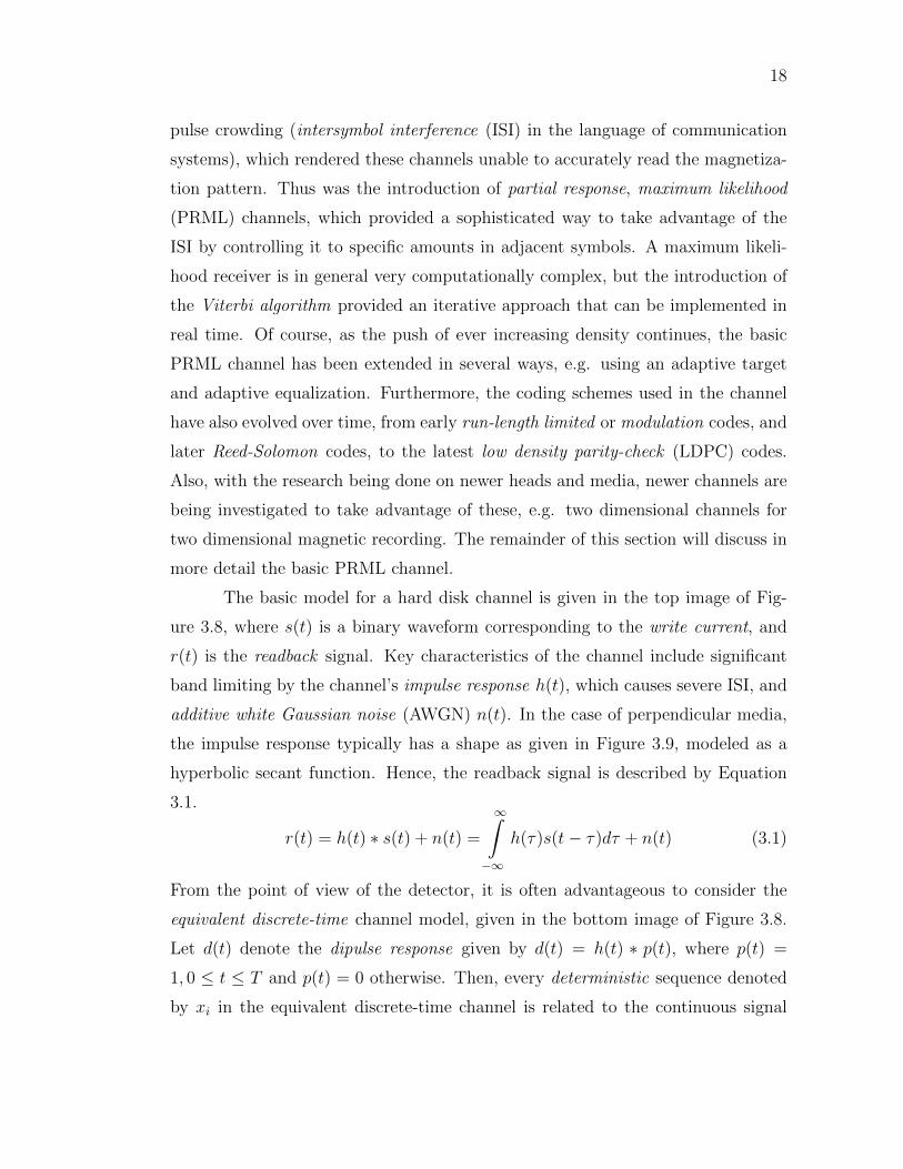
The basic model for a hard disk channel is given in the top image of Fig-
ure 3.8, where s(t) is a binary waveform corresponding to the write current, and
r(t) is the readback signal. Key characteristics of the channel include significant
band limiting by the channel’s impulse response h(t), which causes severe ISI, and
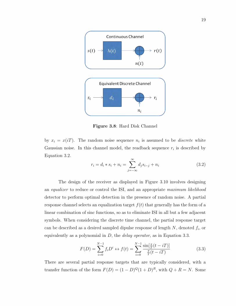
additive white Gaussian noise (AWGN) n(t). In the case of perpendicular media,
the impulse response typically has a shape as given in Figure 3.9, modeled as a
hyperbolic secant function. Hence, the readback signal is described by Equation
3.1.
r(t) = h(t) ∗ s(t) + n(t) =
∞∫−∞
h(τ)s(t− τ)dτ + n(t) (3.1)
From the point of view of the detector, it is often advantageous to consider the
equivalent discrete-time channel model, given in the bottom image of Figure 3.8.
Let d(t) denote the dipulse response given by d(t) = h(t) ∗ p(t), where p(t) =
1, 0 ≤ t ≤ T and p(t) = 0 otherwise. Then, every deterministic sequence denoted
by xi in the equivalent discrete-time channel is related to the continuous signal
19
Figure 3.8: Hard Disk Channel
by xi = x(iT ). The random noise sequence ni is assumed to be discrete white
Gaussian noise. In this channel model, the readback sequence ri is described by
Equation 3.2.
ri = di ∗ si + ni =∞∑
j=−∞
djsi−j + ni (3.2)
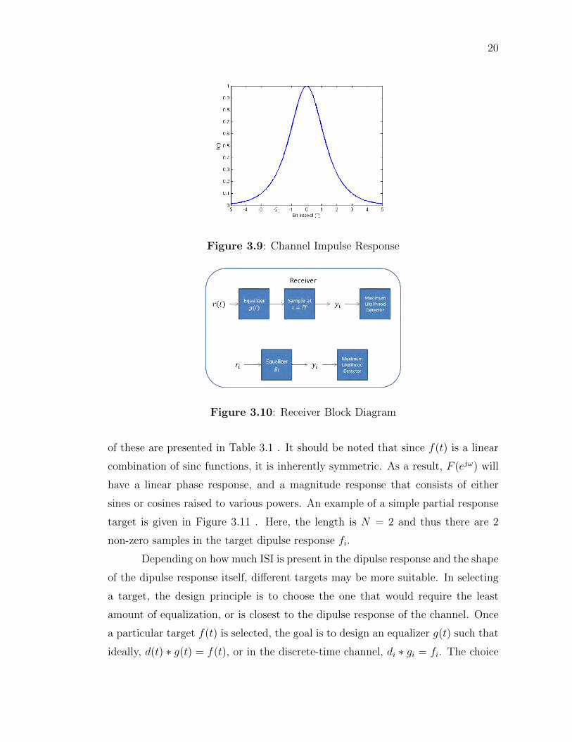
The design of the receiver as displayed in Figure 3.10 involves designing
an equalizer to reduce or control the ISI, and an appropriate maximum likelihood
detector to perform optimal detection in the presence of random noise. A partial
response channel selects an equalization target f(t) that generally has the form of a
linear combination of sinc functions, so as to eliminate ISI in all but a few adjacent
symbols. When considering the discrete time channel, the partial response target
can be described as a desired sampled dipulse response of length N , denoted fi, or
equivalently as a polynomial in D, the delay operator, as in Equation 3.3.
F (D) =N−1∑i=0
fiDi ↔ f(t) =
N−1∑i=0
sin[ πT
(t− iT )]πT
(t− iT )(3.3)
There are several partial response targets that are typically considered, with a
transfer function of the form F (D) = (1−D)Q(1 +D)R, with Q+ R = N . Some
20
Figure 3.9: Channel Impulse Response
Figure 3.10: Receiver Block Diagram
of these are presented in Table 3.1 . It should be noted that since f(t) is a linear
combination of sinc functions, it is inherently symmetric. As a result, F (ejω) will
have a linear phase response, and a magnitude response that consists of either
sines or cosines raised to various powers. An example of a simple partial response
target is given in Figure 3.11 . Here, the length is N = 2 and thus there are 2
non-zero samples in the target dipulse response fi.
Depending on how much ISI is present in the dipulse response and the shape
of the dipulse response itself, different targets may be more suitable. In selecting
a target, the design principle is to choose the one that would require the least
amount of equalization, or is closest to the dipulse response of the channel. Once
a particular target f(t) is selected, the goal is to design an equalizer g(t) such that
ideally, d(t) ∗ g(t) = f(t), or in the discrete-time channel, di ∗ gi = fi. The choice

21
Figure 3.11: Partial Response Class I Target
Table 3.1: List of Common Partial Response Targets
Name Transfer Function fiClass I (PR1) (1 +D) {1, 1}Class II (PR2) (1 +D)2 {1, 2, 1}
Extended Class II (EPR2) (1 +D)3 {1, 3, 3, 1}Twice Extended Class II (E2PR2) (1 +D)4 {1, 4, 6, 4, 1}
Class IV (PR4) (1−D)(1 +D) {1, 0,−1}Extended Class IV (EPR4) (1−D)(1 +D)2 {1, 1,−1,−1}
Twice Extended Class IV (E2PR4) (1−D)(1 +D)3 {1, 2, 0,−2,−1}
22
of using either a discrete-time or continuous-time equalizer (or both) determines
what method is used to design the filter, and if a discrete-time equalizer is chosen,
then the choice between an finite impulse response (FIR) and infinite impulse
response (IIR) equalizer also impacts the design procedure. Usually, a discrete-time
FIR filter is selected for ease of implementation and design; the latter is typically
accomplished using a minimum-mean squared error (MMSE) optimization on the
filter coefficients. Especially if this is made adaptive and the dipulse response is
close enough to the selected target, this can provide excellent results, without the
complication of having to design an optimal IIR filter.
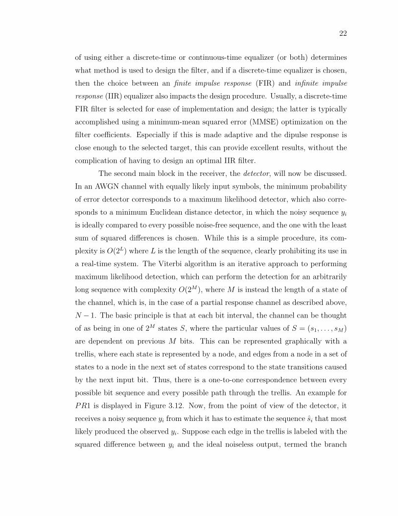
The second main block in the receiver, the detector, will now be discussed.
In an AWGN channel with equally likely input symbols, the minimum probability
of error detector corresponds to a maximum likelihood detector, which also corre-
sponds to a minimum Euclidean distance detector, in which the noisy sequence yi
is ideally compared to every possible noise-free sequence, and the one with the least
sum of squared differences is chosen. While this is a simple procedure, its com-
plexity is O(2L) where L is the length of the sequence, clearly prohibiting its use in
a real-time system. The Viterbi algorithm is an iterative approach to performing
maximum likelihood detection, which can perform the detection for an arbitrarily
long sequence with complexity O(2M), where M is instead the length of a state of
the channel, which is, in the case of a partial response channel as described above,
N − 1. The basic principle is that at each bit interval, the channel can be thought
of as being in one of 2M states S, where the particular values of S = (s1, . . . , sM)
are dependent on previous M bits. This can be represented graphically with a
trellis, where each state is represented by a node, and edges from a node in a set of
states to a node in the next set of states correspond to the state transitions caused
by the next input bit. Thus, there is a one-to-one correspondence between every
possible bit sequence and every possible path through the trellis. An example for
PR1 is displayed in Figure 3.12. Now, from the point of view of the detector, it
receives a noisy sequence yi from which it has to estimate the sequence si that most
likely produced the observed yi. Suppose each edge in the trellis is labeled with the
squared difference between yi and the ideal noiseless output, termed the branch

23
Figure 3.12: Trellis for PR1 Channel
metric. Then, the problem becomes one of finding the shortest path through the
trellis. The Viterbi algorithm comes from the basic observation that the shortest
path through the trellis to node S in stage i + 1 has to be an extension of one
of the shortest paths to each node at stage i. This naturally leads to an iterative
approach, such that for each node at each stage i+ 1, only the shorter of the two
paths (in the binary case) from nodes in stage i is kept, termed the survivor path.
Accounting for initialization and termination stages, this allows the shortest com-
plete path through the entire trellis to be found. During the initialization stages,
the number of nodes at each stage double, while during the termination stages, the
number of nodes halve at each stage. An initial state is assumed, and following
the possible state transitions based on next input bits leads to two possible nodes
in the next stage for every one in the current stage. Also, every path during the
initialization stages is a survivor, since there is only one edge entering each node
in the next stage. In the termination stages, on the other hand, the final state is
assumed, and at each stage the survivors to the remaining nodes are kept.
In summary, a PRML receiver allows accurate detection in severe ISI by
controlling the ISI to a finite number of adjacent symbols using partial response
equalization, and decoding the remaining ISI using an efficient iterative algorithm
to perform maximum likelihood detection in the presence of noise.

24
3.4 Digital Image Processing
Digital imaging is a ubiquitous technology these days and has achieved the
state of being both the cheapest form of capturing images as well as providing high
quality images that can be readily manipulated in software to accomplish a wide
array of tasks. In some cases, such as in electron and scanning probe microscopy,
the resulting images can only be represented digitally–there is no optical image to
begin which that can be captured on film. The key motivation of digital imaging
however, is digital image processing. Once an image is represented digitally, it
can be processed just like any other set of data on a computer. This permits
an endless number of ways to alter images for a variety of different purposes.
Some of the basic types of image processing tasks include enhancement, where
the image is made more visually appealing or usable for a particular purpose,
segmentation, where an image is separated into component parts, and stitching,
where a set of several images related to each other are combined into a composite.
At a higher level, these basic tasks can be used as preprocessing steps to perform
image classification, where the class of the object being imaged is determined, or
pattern recognition, whereby patterns in sets of images are sought that can be used
to group subsets together. Fundamental to all of these is first the representation
of some aspect of the world as a set of numbers–how these numbers are interpreted
determines what the image looks like, and also what meaning can be construed
from them. This section will review the basics of representing images digitally and
methods to perform the stitching of images.
A monotone image I can be described mathematically as a real-valued
function I = f(x, y) of two spatial variables x and y. In order to represent this
image digitally, it first needs to be sampled, and also in order to be stored in
a finite memory, needs to be truncated. This results in a real-valued discrete
function of two integer variables n and m which is non-zero in a finite domain
{n,m|0 ≤ n ≤ N, 0 ≤ m ≤ M}. Finally, it needs to be quantized, which results
in an integer-valued function f [n,m] with a codomain {z ∈ Z|0 ≤ z ≤ 2Q}, for
some integer Q, of the two integer variables n and m. This can be conveniently
represented as a matrix I = [Ii,j] where the ith row and jth column are given by

25
Figure 3.13: Digital Representation of Images
Ii,j = f [j, i], and an element of the matrix is called a pixel. Once the image is
stored on a computer, it can be displayed using a particular choice of colormap,
which is an assignment of a particular shade of gray (or any arbitrary color, for
that matter) to each integer in the codomain of I. An example of this is given in
Figure 3.13. Note that it is possible to remap the integers in the codomain of I
into real quantities, for example using an IEEE 754 Floating-Point representation.
In the MFM images acquired in this work, this is in fact the representation used.
Image stitching is the process of taking a set of images and aligning, trans-
forming, and concatenating them together to form a composite image which dis-
plays a wider view than each of the individual images. In dealing with digital
images, ideally the entire process can be done automatically, without any user
intervention. In practice, providing some information as to the ordering of the
images allows much more efficient stitching. The first step is to decide an appro-
priate motion model to be used as the relationship between the images. Examples
26
include translational, which assumes that each image is related to the others by
a translation, Euclidean, which accounts for rotation and translation, and projec-
tive, which is the most general transformation that preserves straight lines. The
more general the model, the more parameters need to be estimated in the aligning
step. The rest of this section will focus on finding the parameters of a translational
model, which requires that only two parameters, ∆i and ∆j be estimated.
When trying to estimate the parameters of a selected motion model between
a pair of images, a process also called aligning, there are two approaches. One is to
use the pixel values of the two images directly and perform an optimization with
respect to a selected objective function, known as the direct approach. Another
is to first extract features of each image, and perform matching based on these,
and finally estimate the motion parameters from the matched features, termed the
feature-based approach. The latter approach readily allows determining the cor-
respondence between images automatically, but for images where this information
is available, is not justifiable considering the more complex implementation. The
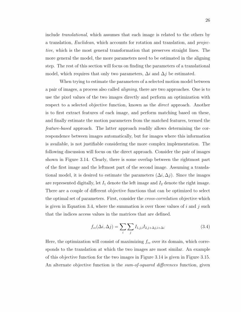
following discussion will focus on the direct approach. Consider the pair of images
shown in Figure 3.14. Clearly, there is some overlap between the rightmost part
of the first image and the leftmost part of the second image. Assuming a transla-
tional model, it is desired to estimate the parameters (∆i,∆j). Since the images
are represented digitally, let I1 denote the left image and I2 denote the right image.
There are a couple of different objective functions that can be optimized to select
the optimal set of parameters. First, consider the cross-correlation objective which
is given in Equation 3.4, where the summation is over those values of i and j such
that the indices access values in the matrices that are defined.
fcc(∆i,∆j) =∑i
∑j
I1,j,iI2,j+∆j,i+∆i (3.4)
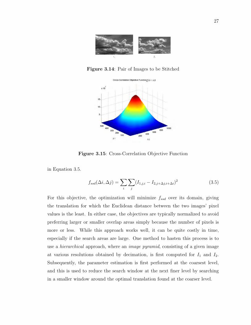
Here, the optimization will consist of maximizing fcc over its domain, which corre-
sponds to the translation at which the two images are most similar. An example
of this objective function for the two images in Figure 3.14 is given in Figure 3.15.
An alternate objective function is the sum-of-squared differences function, given
27
Figure 3.14: Pair of Images to be Stitched
Figure 3.15: Cross-Correlation Objective Function
in Equation 3.5.
fssd(∆i,∆j) =∑i
∑j
(I1,j,i − I2,j+∆j,i+∆i)2 (3.5)
For this objective, the optimization will minimize fssd over its domain, giving
the translation for which the Euclidean distance between the two images’ pixel
values is the least. In either case, the objectives are typically normalized to avoid
preferring larger or smaller overlap areas simply because the number of pixels is
more or less. While this approach works well, it can be quite costly in time,
especially if the search areas are large. One method to hasten this process is to
use a hierarchical approach, where an image pyramid, consisting of a given image
at various resolutions obtained by decimation, is first computed for I1 and I2.
Subsequently, the parameter estimation is first performed at the coarsest level,
and this is used to reduce the search window at the next finer level by searching
in a smaller window around the optimal translation found at the coarser level.

28
3.5 Maximal Length Shift Register Sequences
Pseudorandom sequences have a variety of applications and are useful for
many different purposes. Often, it is important to be able to generate a sequence
that appears random, but is actually computed using a deterministic algorithm
from a given initial state or seed. This might be useful for example to generate
the same sequence at the transmitter and receiver of a digital communication sys-
tem, which nevertheless appears random to all other receivers that do not know
the seed. A particular class of pseudorandom sequences can be efficiently gener-
ated by a shift register with linear feedback and can be shown to satisfy several
randomness properties. Sequences in this class are known as maximal length or
m-sequences, alternatively called pseudonoise or PN sequences. PN sequences are
widely used, for example, in encryption, spread spectrum communications, error
correction coding, global positioning systems, synchronization, impulse response
measurement, and more. They owe their vast utility to their extremely simple gen-
erator implementation, their excellent randomness properties, and their structured
algebraic development. This section will discuss in some more detail these three
aspects of m-sequences.
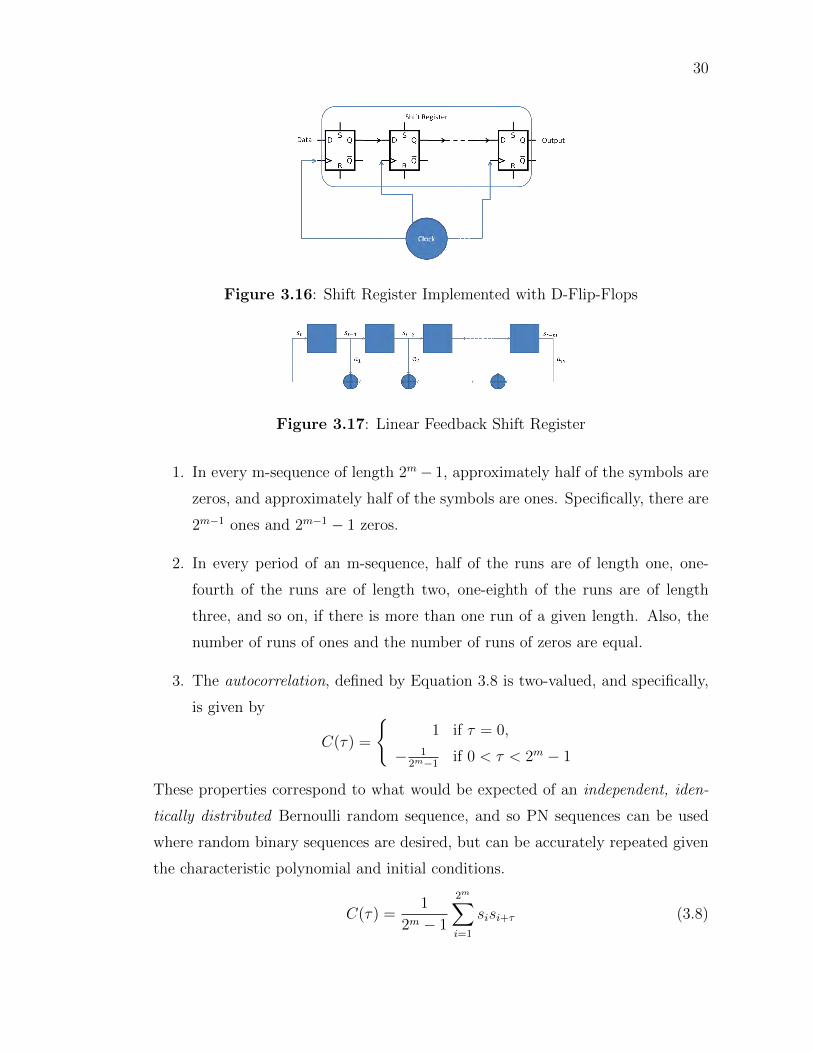
A shift register is a cascade of flip-flops, all driven by a common clock, as
seen in Figure 3.16. The data fed in on one end will thus shift right every clock
cycle, and if no new data is fed in, eventually, all flip-flops will be empty (have all
zeros). Applying feedback to a shift register will allow it to operate continuously,
provided it never reaches the all zeros state. If the feedback consists of taking
the exclusive-or (XOR) of two or more flip-flop outputs and feeding this back to
the input, then this is termed a linear feedback shift register, seen in Figure 3.17.
Finally, a binary sequence can be output from this structure by taking the output of
any of the flip-flops as time progresses, and observing the resulting sequence of bits.
The convention used here will be that the output st will be taken from the input
to the leftmost flip-flop, with the history in the m flip-flops {st−1, st−2, . . . , st−m}.The linear feedback corresponds to imposing a linear recurrence relation between

29
st and its history, i.e. Equation 3.6.
st =m∑i=1
aist−i (3.6)
Note that all the variables and operations here are taken to be in GF (2), that is
the field of integers modulo 2, Z/2Z. An important tool used to study the shift
register sequences with linear feedback is the characteristic polynomial f(x), which
is related to the recurrence relation as given in Equation 3.7.
f(x) = xm −m∑i=1
aixm−i (3.7)
This polynomial captures all the information provided by the recurrence relation
and thus characterizes a particular sequence st. In fact, the property of primitiv-
ity of the polynomial causes the resulting sequence to be a m-sequence. A few
definitions below explain what this means.
Definition 1. Consider the finite field F = GF (pm). A generator of the multi-
plicative group of F (of order pm − 1) is called a primitive root of the field F.
Definition 2. Consider the finite field F = GF (pm) and the prime subfeild Fp =
GF (p). For each α ∈ F , the unique monic polynomial p(x) ∈ Fp[x] which satisfies
p(α) = 0, deg(p(x)) ≤ m, and divides every other polynomial f(x) ∈ Fp[x] that
also has α as a root, is called the minimal polynomial of α with respect to Fp.
Definition 3. Consider the finite field F = GF (pm) and the prime subfeild Fp =
GF (p). If α is a primitive root of F , then the minimal polynomial of α with respect
to Fp is called a primitive polynomial.
Thus, given a primitive polynomial of order m with respect to GF (2), a
m-sequence of length 2m − 1 is uniquely characterized.
Coming to the randomness properties, it can be shown that PN sequences
generated in the above deterministic fashion nonetheless appear very much like
realizations of a true binary random sequence, at least over one period. Specifically,
the following three properties hold.
30
Figure 3.16: Shift Register Implemented with D-Flip-Flops
Figure 3.17: Linear Feedback Shift Register
1. In every m-sequence of length 2m− 1, approximately half of the symbols are
zeros, and approximately half of the symbols are ones. Specifically, there are
2m−1 ones and 2m−1 − 1 zeros.
2. In every period of an m-sequence, half of the runs are of length one, one-
fourth of the runs are of length two, one-eighth of the runs are of length
three, and so on, if there is more than one run of a given length. Also, the
number of runs of ones and the number of runs of zeros are equal.
3. The autocorrelation, defined by Equation 3.8 is two-valued, and specifically,
is given by
C(τ) =
{1 if τ = 0,
− 12m−1
if 0 < τ < 2m − 1
These properties correspond to what would be expected of an independent, iden-
tically distributed Bernoulli random sequence, and so PN sequences can be used
where random binary sequences are desired, but can be accurately repeated given
the characteristic polynomial and initial conditions.
C(τ) =1
2m − 1
2m∑i=1
sisi+τ (3.8)

Chapter 4
MFM Based Data Reconstruction
System
With the necessary background on some of the system design tools described
in Chapter 3, the development of the system to recover data from MFM images
of the surface of a HDD will now be described. Section 4.1 will describe at a
high level the design of the system and the experimental setup used in this work.
Section 4.2 will cover the details of the MFM imaging and various image processing
techniques that are utilized. The design of the PRML channel used to detect data
from the signals acquired from the processed images will be described in Section
4.3. Finally, the performance will be analyzed and methods to improve this will
be discussed in Section 4.4.
4.1 System Overview and Experimental Setup
The system to reconstruct data on a hard disk via MFM imaging is broadly
characterized by three steps. The first is to actually acquire the MFM images on a
portion of the disk of interest, and to collect them in a manner that readily admits
stitching and other future processing. Next is to perform the necessary image pro-
cessing steps (preprocessing, aligning, stitching, and segmenting) to compose all
the images acquired into a single image and separate the different tracks. Finally,
a readback signal is acquired from each track and this is then passed through a
31

32
Figure 4.1: System Block Diagram of MFM Based Data Recovery
PRML channel to give an estimate of the raw data corresponding to the magneti-
zation pattern written on the drive. If the user data is to be recovered, additional
decoding and de-scrambling is required, and the specific ECC, RLL, and scram-
bling parameters of the disk drive must be acquired to perform this. The overall
system is summarized in Figure 4.1.
For the experiments conducted in this work, a special HDD was prepared by
Seagate Technology LLC on which a particular sequence was written bypassing the
usual ECC, RLL coding, scrambling, etc. that is usually performed on user data
before writing it onto the disk. The only operation performed on special sequence
before writing was non-return to zero inverted (NRZI) line coding which was used
to generate the write waveform. The motivation for this is to readily allow com-
parison of any data recovered through this method with the sequence known to
be written to the drive, without needing to reverse engineer or otherwise acquire
the proprietary channel coding parameters. Specifically, the sequence written was
a periodic 256-bit pattern composed of a 255-bit m-sequence appended with one
additional bit. The selected m-sequence st was generated from the primitive poly-
nomial x8 + x6 + x5 + x4 + 1, and the additional bit selected was a 1. The initial
state of the shift register was chosen to be {1, 0, 0, 0, 0, 0, 0, 0}. The full pattern
in hexadecimal notation is given in Table 4.1. The work performed thus far has
focused on attempting to recover data in the un-degaussed case, with the aim of
developing a working system which can be extended to the case of a partially de-
gaussed drive, and the performance in the two cases can then be compared. In the
experiments, all the MFM images were acquired with a Veeco Dimension V SPM,
and all subsequent processing was performed in Matlab.
33
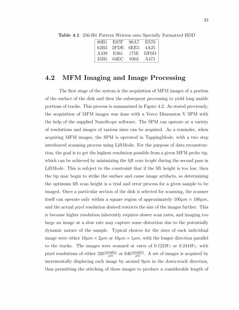
Table 4.1: 256-Bit Pattern Written onto Specially Formatted HDD
80B1 E87F 90A7 D57062B3 2FDE 6EE5 4A25A339 E361 175E DF0D35B5 04EC 9303 A471
4.2 MFM Imaging and Image Processing
The first stage of the system is the acquisition of MFM images of a portion
of the surface of the disk and then the subsequent processing to yield long usable
portions of tracks. This process is summarized in Figure 4.2. As stated previously,
the acquisition of MFM images was done with a Veeco Dimension V SPM with
the help of the supplied NanoScope software. The SPM can operate at a variety
of resolutions and images of various sizes can be acquired. As a reminder, when
acquiring MFM images, the SPM is operated in TappingMode, with a two step
interleaved scanning process using LiftMode. For the purpose of data reconstruc-
tion, the goal is to get the highest resolution possible from a given MFM probe tip,
which can be achieved by minimizing the lift scan height during the second pass in
LiftMode. This is subject to the constraint that if the lift height is too low, then
the tip may begin to strike the surface and cause image artifacts, so determining
the optimum lift scan height is a trial and error process for a given sample to be
imaged. Once a particular section of the disk is selected for scanning, the scanner
itself can operate only within a square region of approximately 100µm × 100µm,
and the actual pixel resolution desired restricts the size of the images further. This
is because higher resolution inherently requires slower scan rates, and imaging too
large an image at a slow rate may capture some distortion due to the potentially
dynamic nature of the sample. Typical choices for the sizes of each individual
image were either 10µm× 2µm or 10µm× 1µm, with the longer direction parallel
to the tracks. The images were scanned at rates of 0.122Hz or 0.244Hz, with
pixel resolutions of either 320 samplesµm
or 640 samplesµm
. A set of images is acquired by
incrementally displacing each image by around 9µm in the down-track direction,
thus permitting the stitching of these images to produce a considerable length of

34
Figure 4.2: Image Acquisition and Processing Stage
a few tracks. Examples of a few raw images, displayed using a default colormap
of the NanoScope program are given in Figure 4.3. Once the raw images are ac-
quired they are represented as a matrix of floating point values corresponding to
the phase difference, measured in degrees, between the cantilever’s oscillation and
the piezoelectric drive. This is exported as a (very large) ASCII text file for further
analysis in Matlab.
Once the images are acquired, there are potentially some degradations that
need to be preprocessed before the stitching can be performed effectively. For
example, some preprocessing steps include hard limiting on images with debris
causing extreme phase values, resizing an image with a slightly different vertical
dimension than the rest, and rotating each image to ensure that the tracks are par-
allel with the image boundaries. As a first step, the parameters of these corrections
were determined manually, but as will be discussed shortly, they can be estimated
automatically as well. Once a given set of images has been preprocessed, the pa-
rameters of the motion model that relates each of the images need to be estimated;
in this case, a translational motion model is used. As mentioned in Section 3.4,
there are two approaches to estimate parametric motion models–pixel based and

35
Figure 4.3: Raw MFM Images of Hard Disk Surface
feature based. A direct approach was employed, and initially a cross-correlation
objective function was selected. To apply this on the full resolution images in a
somewhat timely manner, a heuristic based on the fact that the images nominally
overlap by 1µm is utilized to perform the cross-correlation only on cropped ends
of each pair of images to be stitched. Specifically, for each pair of images, the left
quarter of the right image and the lower half of the right tenth of the left image are
selected and the cross-correlation objective function is maximized over the possible
overlaps of these crops. This process is illustrated more clearly in Figure 4.4. The
resulting optimal point is then converted into appropriate values of the translation
parameters of each image, and they are composed into a single image. Finally, the
center portion of the stitched image is cropped, yielding a set of tracks that are
contiguous throughout the image.
While the procedure described in the previous paragraph is successful at
stitching the images together, it still performs fairly slowly and can be sped up
considerably by using a hierarchical method to estimate the motion parameters. In
this procedure, developed in [Sze06], an image pyramid is computed of each image
to be stitched. The image pyramid consists of a set of images with decreasing
resolution derived from an original image by decimation. The search procedure is
performed at the coarsest level first, and the optimal value obtained thereupon is
used as an estimate to search around in the next finer level. The search window
at the finer level can be much smaller than that at the courser level, thereby
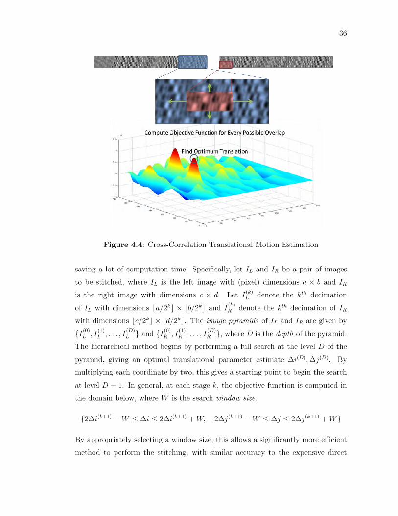
36
Figure 4.4: Cross-Correlation Translational Motion Estimation
saving a lot of computation time. Specifically, let IL and IR be a pair of images
to be stitched, where IL is the left image with (pixel) dimensions a × b and IR
is the right image with dimensions c × d. Let I(k)L denote the kth decimation
of IL with dimensions ba/2kc × bb/2kc and I(k)R denote the kth decimation of IR
with dimensions bc/2kc × bd/2kc. The image pyramids of IL and IR are given by
{I(0)L , I
(1)L , . . . , I
(D)L } and {I(0)
R , I(1)R , . . . , I
(D)R }, where D is the depth of the pyramid.
The hierarchical method begins by performing a full search at the level D of the
pyramid, giving an optimal translational parameter estimate ∆i(D),∆j(D). By
multiplying each coordinate by two, this gives a starting point to begin the search
at level D − 1. In general, at each stage k, the objective function is computed in
the domain below, where W is the search window size.
{2∆i(k+1) −W ≤ ∆i ≤ 2∆i(k+1) +W, 2∆j(k+1) −W ≤ ∆j ≤ 2∆j(k+1) +W}
By appropriately selecting a window size, this allows a significantly more efficient
method to perform the stitching, with similar accuracy to the expensive direct
37
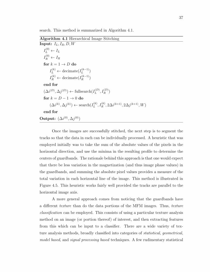
search. This method is summarized in Algorithm 4.1.
Algorithm 4.1 Hierarchical Image StitchingInput: IL, IR, D,W
I(0)L ← IL
I(0)R ← IR
for k = 1→ D do
I(k)L ← decimate(I
(k−1)L )
I(k)R ← decimate(I
(k−1)R )
end for
(∆i(D),∆j(D))← fullsearch(I(D)L , I
(D)R )
for k = D − 1→ 0 do
(∆i(k),∆j(k))← search(I(k)L , I
(k)R , 2∆i(k+1), 2∆j(k+1),W )
end for
Output: (∆i(0),∆j(0))
Once the images are successfully stitched, the next step is to segment the
tracks so that the data in each can be individually processed. A heuristic that was
employed initially was to take the sum of the absolute values of the pixels in the
horizontal direction, and use the minima in the resulting profile to determine the
centers of guardbands. The rationale behind this approach is that one would expect
that there be less variation in the magnetization (and thus image phase values) in
the guardbands, and summing the absolute pixel values provides a measure of the
total variation in each horizontal line of the image. This method is illustrated in
Figure 4.5. This heuristic works fairly well provided the tracks are parallel to the
horizontal image axis.
A more general approach comes from noticing that the guardbands have
a different texture than do the data portions of the MFM images. Thus, texture
classification can be employed. This consists of using a particular texture analysis
method on an image (or portion thereof) of interest, and then extracting features
from this which can be input to a classifier. There are a wide variety of tex-
ture analysis methods, broadly classified into categories of statistical, geometrical,
model based, and signal processing based techniques. A few rudimentary statistical

38
Figure 4.5: Heuristic Method to Segment Tracks
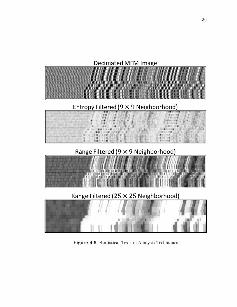
techniques were surveyed, which when combined with additional image processing
tools, namely the Hough transform, provide a method to fit lines to the guardbands
from which the slopes of the tracks can be estimated. Specifically, the statistical
texture analysis techniques of range and entropy filtering were compared. Both
of these perform a neighborhood filtering operation wherein the local statistics–
either range, which measures the range of pixel values, or entropy, which measures
the information entropy–are computed in a given neighborhood of each point of
the image. Performing thresholding on the filtered versions of the images can
identify those regions with smoother texture (corresponding to lower ranges and
entropies) or rougher texture (corresponding to higher ranges and entropies). The
choices of neighborhood size and shape play a significant role in the results of the
filtering–larger neighborhoods are useful for distinguishing larger texture patterns
and vice-versa. An example of the effect of neighborhood size is demonstrated in
Figure 4.6.
It was found that for identifying guardbands, the range operator was more
useful, especially when paired with wide, short neighborhoods (similar to the shape
of the expected guardbands). Using some trial-and-error to determine a “good”
threshold, the low-texture guardbands can be identified, with some other regions
erroneously identified as well. Knowing that the guardbands are expected to be
linear (at least over small dimensions), lines can be fit to the binary image resulting
from thresholding using the Hough transform. This transform parametrizes each
possible line in the image by (ρ, θ), where ρ = x cos(θ) + y sin(θ). Each non-zero
39
Figure 4.6: Statistical Texture Analysis Techniques
40
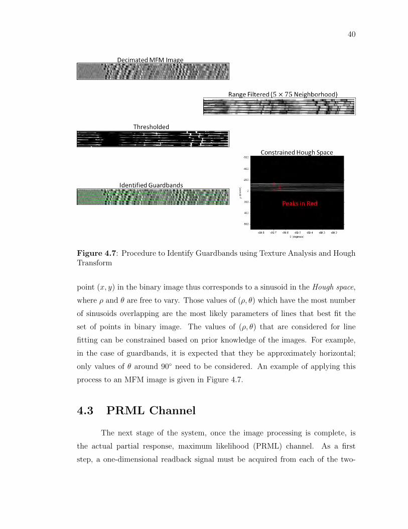
Figure 4.7: Procedure to Identify Guardbands using Texture Analysis and HoughTransform
point (x, y) in the binary image thus corresponds to a sinusoid in the Hough space,
where ρ and θ are free to vary. Those values of (ρ, θ) which have the most number
of sinusoids overlapping are the most likely parameters of lines that best fit the
set of points in binary image. The values of (ρ, θ) that are considered for line
fitting can be constrained based on prior knowledge of the images. For example,
in the case of guardbands, it is expected that they be approximately horizontal;
only values of θ around 90◦ need to be considered. An example of applying this
process to an MFM image is given in Figure 4.7.
4.3 PRML Channel
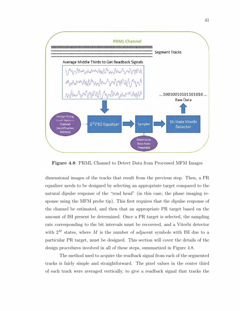
The next stage of the system, once the image processing is complete, is
the actual partial response, maximum likelihood (PRML) channel. As a first
step, a one-dimensional readback signal must be acquired from each of the two-
41
Figure 4.8: PRML Channel to Detect Data from Processed MFM Images
dimensional images of the tracks that result from the previous step. Then, a PR
equalizer needs to be designed by selecting an appropriate target compared to the
natural dipulse response of the “read head” (in this case, the phase imaging re-
sponse using the MFM probe tip). This first requires that the dipulse response of
the channel be estimated, and then that an appropriate PR target based on the
amount of ISI present be determined. Once a PR target is selected, the sampling
rate corresponding to the bit intervals must be recovered, and a Viterbi detector
with 2M states, where M is the number of adjacent symbols with ISI due to a
particular PR target, must be designed. This section will cover the details of the
design procedures involved in all of these steps, summarized in Figure 4.8.
The method used to acquire the readback signal from each of the segmented
tracks is fairly simple and straightforward. The pixel values in the center third
of each track were averaged vertically, to give a readback signal that tracks the

42
changes in phase in the images with an improved signal to noise ratio (SNR). The
form of the resulting signal is similar to that expected from a GMR head flying
over a perpendicular magnetization pattern. Note the constant frequency preamble
portion of the readback signals acquired. This was used in a simple manner to
obtain the oversampling rate of the digitized readback signal, by counting the
number of periods and knowing that each period of the pattern corresponds to
four symbol periods. The more challenging step is to estimate the dipulse response
of the channel, so that an appropriate partial response equalizer can be designed.
To this end, the specially formatted hard drive was written with a known PN
sequence, which permits the use of some channel characterization methods using
the known write waveform and the corresponding readback signal. One particular
method, developed in [Cio86], which uses a least-squares approach to performing
the necessary deconvolution was selected.
To describe this method, the following notation will be used. Let r(t) be
the readback signal given by Equation 4.1, where si is the ith binary data value,
d(t) is the dipulse response, and n(t) is white Gaussian noise. If this is sampled at
an oversampling rate Td = T/n, n > 1, the resulting sequence is given in Equation
4.2. Suppose the oversampled readback signal r[m] along with the binary data
si is available over a finite number of bit periods, i = 0, . . . , N . The goal of the
channel characterization is to produce an estimate of the dipulse response d[m]
such that the resulting readback signal estimate r[m] is as close as possible to the
observed r[m]. Defining e[m] = r[m] − r[m] and choosing the find the d[m] that
minimizes∑L
m=0 e2[m], for some order L, results in a least-squares optimization
problem. Note that the optimal solution will depend on the order L and will be
denoted dL[m]. This has the closed-form solution given in Equation 4.4, where
the appropriate vectors are related to the finite length sequences by Equation 4.3.
Note that there are n− 1 zeros between entries in the vector sN,i.
r(t) =∞∑
i=−∞
sid(t− iT ) + n(t) (4.1)
r[m] , r(mTd) =∞∑
i=−∞
sid(mTd − iT ) + n(mTd) (4.2)
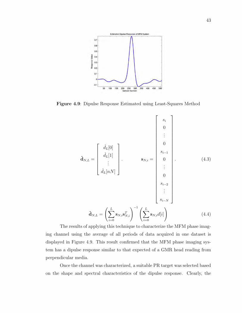
43
Figure 4.9: Dipulse Response Estimated using Least-Squares Method
dN,L =
dL[0]
dL[1]...
dL[nN ]
. sN,i =
si
0...
0
si−1
0...
0
si−2
...
si−N
. (4.3)
dN,L =
(L∑i=0
sN,isTN,i
)−1( L∑i=0
sN,id[i]
)(4.4)
The results of applying this technique to characterize the MFM phase imag-
ing channel using the average of all periods of data acquired in one dataset is
displayed in Figure 4.9. This result confirmed that the MFM phase imaging sys-
tem has a dipulse response similar to that expected of a GMR head reading from
perpendicular media.
Once the channel was characterized, a suitable PR target was selected based
on the shape and spectral characteristics of the dipulse response. Clearly, the
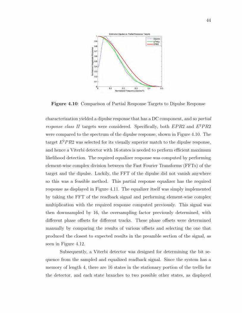
44
Figure 4.10: Comparison of Partial Response Targets to Dipulse Response
characterization yielded a dipulse response that has a DC component, and so partial
response class II targets were considered. Specifically, both EPR2 and E2PR2
were compared to the spectrum of the dipulse response, shown in Figure 4.10. The
target E2PR2 was selected for its visually superior match to the dipulse response,
and hence a Viterbi detector with 16 states is needed to perform efficient maximum
likelihood detection. The required equalizer response was computed by performing
element-wise complex division between the Fast Fourier Transforms (FFTs) of the
target and the dipulse. Luckily, the FFT of the dipulse did not vanish anywhere
so this was a feasible method. This partial response equalizer has the required
response as displayed in Figure 4.11. The equalizer itself was simply implemented
by taking the FFT of the readback signal and performing element-wise complex
multiplication with the required response computed previously. This signal was
then downsampled by 16, the oversampling factor previously determined, with
different phase offsets for different tracks. These phase offsets were determined
manually by comparing the results of various offsets and selecting the one that
produced the closest to expected results in the preamble section of the signal, as
seen in Figure 4.12.
Subsequently, a Viterbi detector was designed for determining the bit se-
quence from the sampled and equalized readback signal. Since the system has a
memory of length 4, there are 16 states in the stationary portion of the trellis for
the detector, and each state branches to two possible other states, as displayed

45
Figure 4.11: Required Partial Response Equalizer
Figure 4.12: Sampled and Equalized Readback Signal

46
Figure 4.13: Sixteen Stage Trellis for E2PR4 Channel
in Figure 4.13. During each iteration of the algorithm, the path lengths of the
two possible paths to each node are calculated and the shortest one is stored. Ini-
tial and final values of -1 are assumed, and there are 4 initialization stages and 4
termination stages in which the trellis grows or shrinks respectively.
4.4 Performance Analysis
As discussed previously, the experiments performed using the HDD specially
prepared with the extended periodic PN sequence allows the comparison of raw
data detected via the approach described in Section 4.3 to what is known to be the
written raw data. While at the simplest level, merely computing the number of
bits incorrectly detected gives a good metric of performance, it is also informative
to look at the error events themselves. Given a particular partial response channel
model, certain error events are more likely than others, and this should be apparent
in the relative frequencies of the observed error events as well. This section will
discuss some of the empirically observed bit error rates and error event frequencies.
An example of the comparison between the known bit pattern and the
detected sequence in one period of one track of one dataset is shown in Figure

47
4.14. Visually, it is seen the that two sequences are quite similar; performing a
bitwise comparison however yields an error rate of 25.8%! In fact, this is a trend
seen across multiple periods in multiple tracks, summarized in Table 4.2. Looking
at this a little closer, it is seen that the nature of errors seems to involve the
deletion or insertion of bits at random locations, shifting all subsequent bits for
a long run. To perform a more thorough analysis of these phenomena, the error
events were analyzed, using a method developed in [WAW97]. Let si denote the
actual written binary sequence and si denote the estimate of si at the output of
the Viterbi detector. The input error sequence es,i is defined by es,i = si − si, and
the output error sequence ey,i is defined by ey,i = di ∗es,i. An error event λ extends
from i1 to i2 if the following three properties hold, where N is the order of the
partial response target.
1. es,i1−i = 0 for all 0 < i ≤ N
2. es,i1 6= 0
3. i2 is the smallest i ≥ i1 for which es,i−j = 0 for all 0 ≤ j < N
The squared (or Euclidean) distance d2(λ) of an error event is then defined as
follows.
d2(λ) =
i2∑i=i1
e2y,i
For a particular partial response channel, the possible error events and correspond-
ing Euclidean distances can be determined by first forming what is known as the
error state diagram, which is a labeled directed graph in which a particular error
event is a path whose squared distance can be computed by summing the labels
on each edge of the path.
For the E2PR2 channel, taking si ∈ {−1, 1} means that es,i ∈ {−2, 0, 2},which will be abbreviated as {−, 0,+}. The error state diagram will contain 34 =
81 states, an this can be represented for the purpose of computation by a pair of
81× 81 matrices–one for adjacency and one for the labels. The distance spectrum
of the E2PR2 channel was computed using a depth-first search (DFS) on the
error state diagram. The error events are tabulated in Table 4.3–note that for
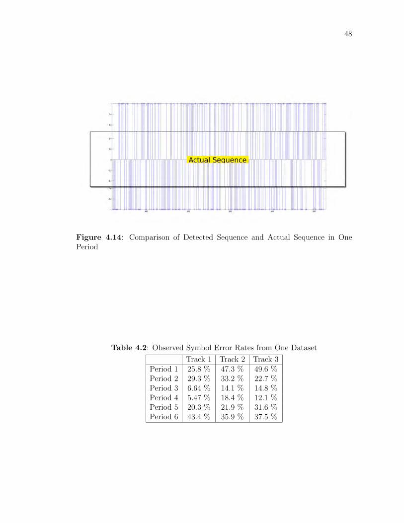
48
Figure 4.14: Comparison of Detected Sequence and Actual Sequence in OnePeriod
Table 4.2: Observed Symbol Error Rates from One Dataset
Track 1 Track 2 Track 3Period 1 25.8 % 47.3 % 49.6 %Period 2 29.3 % 33.2 % 22.7 %Period 3 6.64 % 14.1 % 14.8 %Period 4 5.47 % 18.4 % 12.1 %Period 5 20.3 % 21.9 % 31.6 %Period 6 43.4 % 35.9 % 37.5 %
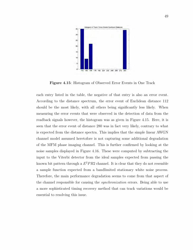
49
Figure 4.15: Histogram of Observed Error Events in One Track
each entry listed in the table, the negative of that entry is also an error event.
According to the distance spectrum, the error event of Euclidean distance 112
should be the most likely, with all others being significantly less likely. When
measuring the error events that were observed in the detection of data from the
readback signals however, the histogram was as given in Figure 4.15. Here, it is
seen that the error event of distance 280 was in fact very likely, contrary to what
is expected from the distance spectra. This implies that the simple linear AWGN
channel model assumed heretofore is not capturing some additional degradation
of the MFM phase imaging channel. This is further confirmed by looking at the
noise samples displayed in Figure 4.16. These were computed by subtracting the
input to the Viterbi detector from the ideal samples expected from passing the
known bit pattern through a E2PR2 channel. It is clear that they do not resemble
a sample function expected from a bandlimited stationary white noise process.
Therefore, the main performance degradation seems to come from that aspect of
the channel responsible for causing the synchronization errors. Being able to use
a more sophisticated timing recovery method that can track variations would be
essential to resolving this issue.

50
Table 4.3: Error Events for E2PR2 upto d2 = 280
Distance d2(λ) Input Error Events λ112 {−,+}160 {−,+,−,+}168 {−,+,−}176 {−,+, 0, 0,−,+}192 {−,+, 0,−, 0,+,−}224 {−,+,−, 0, 0,−,+}, {−,+, 0, 0,−,+,−,+}
232{−, 0,+,−}, {−,+,−, 0, 0,+,−}, {−,+,−,+, 0,−, 0,+,−},
{−,+, 0,−}, {−,+, 0,−, 0,+,−,+,−},{−,+, 0, 0,−,+,−}, {−,+, 0, 0, 0,+,−}
240{−,+,−, 0,+, 0,−,+}, {−,+, 0,−, 0,+,−,+},
{−,+, 0, 0,−,+, 0, 0,−,+}256 {−,+, 0,−, 0,+,−, 0, 0,+,−}, {−,+, 0, 0,−,+, 0,−, 0,+,−}
272{−, 0,+,−,+,−}, {−,+,−,+, 0,−},
{−,+,−,+, 0,−,+,−,+,−}, {−,+,−,+, 0, 0,−,+,−,+},{−,+, 0,−, 0,+,−, 0,+, 0,−,+}, {−,+, 0, 0,+,−}
280
{−}, {−, 0,+,−,+}, {−,+,−, 0, 0,+,−,+,−},{−,+,−, 0,+, 0,−,+,−,+}, {−,+,−, 0,+},
{−,+,−,+, 0,−, 0,+,−,+}, {−,+,−,+, 0, 0,−,+,−},{−,+,−,+, 0, 0, 0,+,−}, {−,+, 0, 0, 0,+,−,+,−}
Figure 4.16: “Noise” Samples from Six Periods of One Track

Chapter 5
Extensions and Further Analysis
In the performance analysis discussion in Section 4.4, it was noted that the
main source of degradation was from the varying bit timing that was not accounted
for when sampling the equalized readback signals. Typically, in the read channel
of an actual hard disk drive, a phase-locked loop (PLL) is employed to perform
bit synchronization. However, in the case of the readback signals coming from
MFM images, there is typically only a small segment of the constant frequency
preamble available, over which a PLL would not be able to lock, much less track
timing variations. Also, the amount of the bit timing variation is more significant
than on a typical HDD, especially considering the minute dimensions of each set
of images. This situation provided the motivation to investigate the use of time-
frequency (TF) analysis methods on the readback signals, to determine if these bit
timing variations–which intuitively should manifest a varying spectral content–can
be characterized and compensated for. Section 5.1 describes the specific analysis
techniques used and their results, while Section 5.2 displays an interesting property
of m-sequences that was observed in the TF analysis of the readback signals.
5.1 Time-Frequency Analysis Methods
From basic signals and systems theory, there are two domains in which a
signal can be analyzed and understood–time and frequency. Traditional Fourier
analysis provides the bridge between these two domains. The Fourier transform
51

52
takes a time domain signal and returns a frequency domain spectrum, while the
inverse Fourier transform does the opposite. Thinking of signals as vectors in an
abstract vector space, the Fourier transform essentially projects a time domain
signal onto a basis of sinusoids, while the inverse Fourier transform reconstructs
the original signal from its representation in the Fourier basis. While this fre-
quency analysis does provide useful insights into the behavior of signals, it does
so in a manner that removes all time information (since the sinusoids are of infi-
nite length). Signals that have time-varying frequency content, however, cannot
readily be analyzed in either the time or frequency domains alone, and thus more
sophisticated signal analysis methods are needed. These fall under the broad class
of time-frequency analysis methods, which are the focus of this section.
Consider a pure linear chirp signal of the form cos(2π(at+ b)t), which has
a frequency that changes linearly with time. A plot of an example of this signal
and the magnitude of its Fourier transform is given in Figure 5.1. It is seen that
although the spectrum has a wider bandwidth due to the chirping of the signal,
the time-varying frequency information is not captured by the Fourier transform.
This is an example of a signal for which time-frequency analysis methods would
be useful. One of the seminal papers on this topic was the 1946 Theory of Com-
munication by Dennis Gabor [Gab46]. There he develops the logon transform and
considers the analysis of signals in time-frequency space. The logon transform uses
a set of basis functions that are Gaussian-windowed sinusoids, of the form given
in Equation 5.1, which have a finite span in both time and frequency. This allows
the representation of a signal in both time and frequency, and is therefore useful
to view time-varying spectral content. One important parameter to select is the
length of the window, which is inversely proportional to α. A longer window gives
better frequency resolution at the expense of time resolution, and vice versa. The
logon transform has been generalized to the short-time or sliding-window Fourier
transform, which uses an arbitrary window shape rather than a Gaussian. A plot of
the spectrogram, or time-frequency distribution (TFD) of a pure chirp is displayed
in Figure 5.2. Thus, unlike in the Fourier transform of the pure chirp in Figure
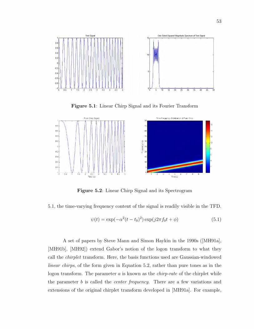
53
Figure 5.1: Linear Chirp Signal and its Fourier Transform
Figure 5.2: Linear Chirp Signal and its Spectrogram
5.1, the time-varying frequency content of the signal is readily visible in the TFD.
ψ(t) = exp(−α2(t− t0)2) exp(j2πf0t+ φ) (5.1)
A set of papers by Steve Mann and Simon Haykin in the 1990s ([MH91a],
[MH91b], [MH92]) extend Gabor’s notion of the logon transform to what they
call the chirplet transform. Here, the basis functions used are Gaussian-windowed
linear chirps, of the form given in Equation 5.2, rather than pure tones as in the
logon transform. The parameter a is known as the chirp-rate of the chirplet while
the parameter b is called the center frequency. There are a few variations and
extensions of the original chirplet transform developed in [MH91a]. For example,
54
these include the adaptive chirplet transform, discussed in [MH91b] and [MH92],
wherein a small set of basis functions are adapted using an iterative algorithm to
fit the TFD of the original signal as well as possible, instead of projecting a signal
directly onto the basis functions, which yields an output in a high dimensional
space and is difficult to analyze. This was in fact the method investigated as a
potential way to determine how much a readback signal has been chirped through
the MFM phase imaging process.
ψ(t) = exp(−α2(t− t0)2) exp(j2π(at+ b)t+ φ) (5.2)
The adaptive chirplet transform models the time-frequency distribution of
a signal as a probability density function which is then approximated by a mix-
ture of Gaussians. A standard algorithm for fitting a Gaussian mixture model is
the expectation maximization (EM) algorithm [DLR77]. This was adapted to be
used on TFDs in [MH92], where it is termed the logon expectation maximization
(LEM) algorithm. Running the LEM algorithm allows the user to select a num-
ber of Gaussians to be used, and the parameters of each, namely the means and
covariance matrices, are learned from the TFD of a signal of interest. The adap-
tive chirplet transform uses each of these Gaussians to determine a corresponding
chirplet basis function, whose parameters, e.g. center frequency b and chirp-rate
a, can be computed from the parameters of the Gaussian. An example of running
LEM on a synthetic signal is given in Figure 5.3.
The chirping degradation imposed by the channel is modeled as in Figure
5.4. The parameters of this model are the chirpiness α and the starting scale β.
The goal of using the adaptive chirplet transform is to estimate the parameters of
this model from the readback signals directly. Provided that the input signal to
the channel has a flat TFD, it is expected that the determining the chirpiness of
the channel should be possible from applying the adaptive chirplet transform with
a single Gaussian to the output. One thing to note is that for a rich input signal
with a relatively flat power spectrum, each frequency component is chirped with
a different chirp-rate. This means care must be taken when using the adaptive
chirplet transform to estimate the chirpiness, since it estimates a particular chirp-
rate and center frequency. One simple way to get an estimate of the chirpiness is

55
Figure 5.3: Application of LEM Algorithm to Test Signal

56
Figure 5.4: Chirping Degradation Model
to divide the chirp-rate by center frequency. This procedure was used to analyze
a signal with synthesized chirping degradation. It was found to estimate the syn-
thesized chirpiness with reasonable accuracy, as summarized in Figure 5.5. Note
the radial stretching of the TFD due to the chirping degradation, as opposed to a
simple rotation.
Applying this technique to the readback signals acquired from the MFM
images has not yet proven to be fruitful. One reason seems to stem from the
fact that the chirping distortion, although significant enough to adversely affect
bit timing, does not seem to be clearly visible in the TFD, as seen in Figure
5.6. Another cause is due to the inherently time-varying frequency contents of the
periodic extended PN sequence that seem to be captured by the adaptive chirplet
transform, instead of the degradation due to the channel alone. Nevertheless,
time-frequency analysis techniques do seem to be the appropriate tools to use in
analyzing degradations of this form, and perhaps methods other than the adaptive
chirplet transform are more suitable for the specific constraints imposed by the
readback signals.
5.2 Precoding of PN Sequences
When utilizing the TF analysis discussed in Section 5.1 on the readback
signals, initially it was found that there was a large chirp-rate picked up by the
adaptive chirplet transform, especially if LEM was performed on a segment of the
readback signal (covering one period, for example). To investigate this a bit further,
it was decided to perform the TF analysis on synthesized m-sequences, in order to

57
Figure 5.5: Chirpiness Estimation using LEM on Synthetic Signal
Figure 5.6: Time-Frequency Distribution of Readback Signal
58
determine if there are some inherent time-varying characteristics of PN sequences.
Also, as mentioned in 4.1, since non-return to zero inverted (NRZI) precoding was
employed in the recording system, the effects of this precoding on m-sequences
and subsequently their time-frequency characteristics was investigated. It was
observed that in fact, performing NRZI precoding on a PN sequence resulted in a
shifted and potentially complemented version of the original. It turns out this is
actually a general result, not widely discussed, but does appear in some technical
reports [Sha] and the peer-reviewed literature [RTM01]. This section will discuss
this result in some more detail, provide a different version of the proof than does
[RTM01], and provide some examples.
Given a sequence st, the NRZI precoding operation (also called differential
encoding in digital communications literature) produces the sequence ut defined
by Equation 5.3. Note that this operation can also be defined as the solution to
the difference equation given in Equation 5.4. Using the notation established in
Section 3.5, consider st to be a PN sequence produced by a linear feedback shift
register with the primitive characteristic polynomial f(x) = xm−∑m
i=1 aixm−i and
satisfying the linear recursion st =∑m
i=1 aist−i. Note that as discussed in [McE87],
with the help of the field trace function from GF (q) to GF (qm), the PN sequence
can be written as st = Tr(θαt). Here θ ∈ GF (qm) and α is a root of the primitive
polynomial f(x). Now, the following theorem precisely describes the general result.
ut =t∑i=0
st (5.3)
ut = ut−1 + st (5.4)
Theorem 5.1. Given a PN sequence st, the precoded version ut is either a cyclic
shift of the original, i.e. ut = st+i, or the complement of a cyclic shift of the
original, i.e. ut = 1 + st+i , st+i. Furthermore, this shift value can be determined
based on the primitive polynomial producing the sequence, and is independent of
the starting point of the precoder.
Proof. First, the fact that ut = st+i or ut = st+i will be shown. Note that using
the fact that st satisfies the recursion and replacing it in the precoder definition

59
5.3 gives the following.
ut =t∑
k=0
m∑i=1
aisk−i
Changing the order of summation and factoring ai from the inner sum gives that
ut =m∑i=1
ai
t∑k=0
sk−i
Replacing the variable k with j+ i in the second sum results in the next equation.
ut =m∑i=1
ai
t−i∑j=−i
sj
Breaking the second sum into two parts yields that
ut =m∑i=1
ai
t−i∑j=0
sj +m∑i=1
ai
−1∑j=−i
sj
Noting that the second term is independent of t and defining d ,∑m
i=1 ai∑−1
j=−i sj
gives the following.
ut =m∑i=1
ai
t−i∑j=0
sj + d
Finally, noticing that the inner sum is just ut−i shows that
ut =m∑i=1
aiut−i + d
Thus, ut satisfies the same linear recursion as st, upto a complement d. Since it
satisfies the same recursion, it must be the same PN sequence, with a shift. Now,
to determine the particular shift value i, the field trace representation is used.
Here, α is taken to be α = x mod f(x), where f(x) is the primitive polynomial
associated with the recurrence relation of the m-sequence. Assuming, without loss
of generality, that ut and st satisfy the linear recursion (note that if ut does not,
ut does), we have the following equations, for some θ and θ ∈ GF (2m).
st = Tr(θαt)
ut = Tr(θαt)

60
Note that since α generates GF (2m), the above can be written as follows, for some
0 ≤ l < m.
st = Tr(αl)
ut = Tr(αl+i)
Now, utilizing the fact that st and ut are related by the precoding operation yields
Tr(αl+i) + Tr(αl+i−1) = Tr(αl)
Using the linearity and injectiveness of the field trace function (see [McE87]), it
follows that
αl(αi + αi−1) = αl
Performing some simple manipulation yields
αi = α(1 + α)−1 (5.5)
This is an equation that is readily solved using e.g. a table of Galois fields for i.
Since α depends only on the choice of f(x), and not on θ, it is seen that this shift
value is independent of the starting shift of the precoder.
Another thing to note in light of this theorem is that the factor d, defined by
Equation 5.6, is a function of the initial values of the shift register st,−m ≤ t ≤ −1
and the tap weights ai of the linear feedback. Note that this sum can be rewritten
as in Equation 5.7. Consider what happens if the precoder is applied to advanced
versions of st. This results in d varying since the initial values in the shift register
are changing. Defining this sequence of complements as dt, it is seen that, applying
Equation 5.7, this sequence can be expressed as in Equation 5.8. Notice that the
inner sum is a sum of a subset of the tap weights, and so dt is a sum of shifted
versions of st. Hence, by the cycle-and-add property of m-sequences, it is seen that
dt is itself an m-sequence, and in particular, is a shift of st.
d =m∑i=1
ai
−1∑j=−i
sj (5.6)
=m∑j=1
s−j
m∑i=j
ai (5.7)

61
dt =m∑j=1
st−j
m∑i=j
ai (5.8)
Example 5.1. As a first example, consider m = 3, f(x) = x3+x+1, and the initial
states {s−3, s−2, s−1} = {0, 0, 1}. Here the tap weights are {a1, a2, a3} = {0, 1, 1}and the recurrence relation is st = st−2 + st−3. Computing st and ut gives the
values below. Note that here d is 1, as computed below, and so ut is st−2. Also,
the sequence of complements here is simply dt = st−3, since all other coefficients
are zero.
{st} = {0, 0, 1, 0, 1, 1, 1}
{ut} = {0, 0, 1, 1, 0, 1, 0}
{ut} = {1, 1, 0, 0, 1, 0, 1}
d = (a1 + a2 + a3)s−1 + (a2 + a3)s−2 + a3s−3 = s−3 = 1
Example 5.2. For another example, consider m = 4, f(x) = x4+x+1, and the ini-
tial states {s−4, s−3, s−2, s−1} = {0, 0, 0, 1}. Here the tap weights are {a1, a2, a3, a4} =
{0, 0, 1, 1} and the recurrence relation is st = st−3 + st−4. Computing st and ut
gives the values below. Note that here d is 1, as computed below, and so ut = st−3.
Again, the sequence of complements here is simply dt = st−4.
{st} = {0, 0, 0, 1, 0, 0, 1, 1, 0, 1, 0, 1, 1, 1, 1}
{ut} = {0, 0, 0, 1, 1, 1, 0, 1, 1, 0, 0, 1, 0, 1, 0}
{ut} = {1, 1, 1, 0, 0, 0, 1, 0, 0, 1, 1, 0, 1, 0, 1}
d = (a1 + a2 + a3 + a4)s−1 + (a2 + a3 + a4)s−2 + (a3 + a4)s−3 + s−4 = s−4 = 1
Based on the above examples, there appears to be a trend, also noted in
[Sha], that for PN sequences generated from polynomials of the form xm+x+1, the
resulting shift of the precoded sequence is m−1, and the sequence of complements
dt = st−m. This can be verified by solving Equation 5.5.

Chapter 6
Conclusion
In conclusion, as was presented in the previous chapters, a system to recover
data from a hard disk drive through magnetic force microscopy was developed to
do so from an un-degaussed hard disk under certain experimental conditions. The
design of this system took inspiration from the read channels of modern hard disk
drives to accomplish this goal. The performance has been poor even under these
idealized conditions, but this is attributed to a particular form of degradation that
could be removed by an improved experimental setup. Techniques to remove this
degradation via signal processing were investigated, and while they have not proven
successful yet, they still hold promise to be beneficial. Since the performance
of the developed system has been poor even when recovering data from an un-
degaussed hard disk drive, any amount of degaussing would make this system
unable to recover data. It should be emphasized that even if high performance
could be achieved in detecting data from the images, the time required for the
imaging process itself would make the recovery of any significant amounts of data
intractable.
This having been said, it is interesting that the response of magnetic force
microscopy to the magnetization pattern has enough similarities to that of a read
head to allow the application of the design principles in read channels to this work.
As the technology in both microscopy and hard disk drives evolves, the questions
this work has sought to answer and the answers this thesis has provided might yet
change. Ultimately, only time will tell.
62
Bibliography
[Cio86] J.M. Cioffi. Least-squares storage-channel identification. IBM Journalof Research and Development, 30(3):310–320, 1986.
[DLR77] A. P. Dempster, N. M. Laird, and D. B. Rubin. Maximum likeli-hood from incomplete data via the em algorithm. JOURNAL OF THEROYAL STATISTICAL SOCIETY, SERIES B, 39(1):1–38, 1977.
[Gab46] D. Gabor. Theory of communication. part 1: The analysis of infor-mation. Electrical Engineers - Part III: Radio and CommunicationEngineering, Journal of the Institution of, 93(26):429–441, 1946.
[GS03] S.L. Garfinkel and A. Shelat. Remembrance of data passed: a study ofdisk sanitization practices. Security Privacy, IEEE, 1(1):17–27, 2003.
[HCC09] G.F. Hughes, T. Coughlin, and D.M. Commins. Disposal of disk andtape data by secure sanitization. Security Privacy, IEEE, 7(4):29–34,2009.
[KMFC04] Sashi K. Kasanavesi, Tom D. Milster, David Felix, and Taeyoung Choi.Data recovery from a compact disc fragment. In Proceedings of SPIE,volume 5380, pages 116–127, 2004.
[McE87] Robert J. McEliece. Finite Fields for Computer Scientists and Engi-neers. Kluwer Academic Publishers, 1987.
[MH91a] Steve Mann and Simon Haykin. The chirplet transform: A generaliza-tion of Gabor’s logon transform. Vision Interface ’91, pages 205–212,June 3-7 1991. ISSN 0843-803X.
[MH91b] Steve Mann and Simon Haykin. The Adaptive Chirplet: An AdaptiveWavelet Like Transform. SPIE, 36th Annual International Symposiumon Optical and Optoelectronic Applied Science and Engineering, 21-26July 1991.
[MH92] Steve Mann and Simon Haykin. Adaptive “Chirplet” Transform: anadaptive generalization of the wavelet transform. Optical Engineering,31(6):1243–1256, June 1992.
63

64
[RTM01] M. Rice, S. Tretter, and P. Mathys. On differentially encoded m-sequences. Communications, IEEE Transactions on, 49(3):421–424,2001.
[Sha] Hari Shankar. Duobinary modulation for optical systems. Technicalreport, Inphi Corporation.
[Sob04] Charles H. Sobey. Recovering unrecoverable data: The need for drive-independent data recovery. Technical report, ChannelScience, 2004.
[SOS06] C.H. Sobey, L. Orto, and G. Sakaguchi. Drive-independent data recov-ery: the current state-of-the-art. Magnetics, IEEE Transactions on,42(2):188–193, 2006.
[Sze06] Richard Szeliski. Image alignment and stitching: A tutorial. TechnicalReport MSR-TR-2004-92, Interactive Visual Media Group, MicrosoftResearch, December 2006.
[TKM+05] Chun Tse, Charles Krafft, Isaak Mayergoyz, Patrick McAvoy, andChun-Yang Tseng. Forensic recovery of hard disk data by using thespin-stand imaging technique. In Proceedings of SPIE, volume 5778,pages 595–606, 2005.
[WAW97] A.D. Weathers, S.A. Altekar, and J.K. Wolf. Distance spectra forPRML channels. Magnetics, IEEE Transactions on, 33(5):2809–2811,1997.