electronic engineering and computing technology · ing, high performance computing, and industrial...
TRANSCRIPT

Electronic Engineering and Computing Technology

Lecture Notes in Electrical Engineering
Volume 60
For further volume:http://www.springer.com/series/7818

Sio-Iong Ao • Len GelmanEditors
Electronic Engineeringand Computing Technology
123

EditorsDr. Sio-Iong AoInternational Association of EngineersUnit 1, 1/F37-39 Hung To Road, Hong [email protected]
Professor Len GelmanCranfield UniversitySchool of EngineeringDept. Process & Systems EngineeringCranfield, BedsUnited Kingdom MK43 0AL
ISSN 1876-1100ISBN 978-90-481-8775-1 e-ISBN 978-90-481-8776-8DOI 10.1007/978-90-481-8776-8Springer Dordrecht Heidelberg London New York
Library of Congress Control Number: 2010925339
c© Springer Science+Business Media B.V. 2010No part of this work may be reproduced, stored in a retrieval system, or transmitted in any form or byany means, electronic, mechanical, photocopying, microfilming, recording or otherwise, without writtenpermission from the Publisher, with the exception of any material supplied specifically for the purposeof being entered and executed on a computer system, for exclusive use by the purchaser of the work.
Printed on acid-free paper
Springer is part of Springer Science+Business Media (www.springer.com)

Preface
A large international conference in Electronic Engineering and ComputingTechnology was held in London, UK, July 1–3, 2009, under the World Congresson Engineering (WCE 2009). The WCE 2009 was organized by the Interna-tional Association of Engineers (IAENG); the Congress details are available at:http://www.iaeng.org/WCE2009. IAENG is a non-profit international associationfor engineers and computer scientists, which was founded originally in 1968. TheWorld Congress on Engineering serves as good platforms for the engineering com-munity to meet with each other and exchange ideas. The conferences have alsostruck a balance between theoretical and application development. The conferencecommittees have been formed with over 200 members who are mainly researchcenter heads, faculty deans, department heads, professors, and research scientistsfrom over 30 countries. The conferences are truly international meetings with ahigh level of participation from many countries. The response to the Congress hasbeen excellent. There have been more than 800 manuscript submissions for theWCE 2009. All submitted papers have gone through the peer review process, andthe overall acceptance rate is 57%.
This volume contains 61 revised and extended research articles written by promi-nent researchers participating in the conference. Topics covered include ControlEngineering, Network Management, Wireless Networks, Biotechnology, SignalProcessing, Computational Intelligence, Computational Statistics, Internet Comput-ing, High Performance Computing, and industrial applications. The book offers thestate of the art of tremendous advances in electronic engineering and computingtechnology and also serves as an excellent reference work for researchers and grad-uate students working on electronic engineering and computing technology.
International Association of Engineers Dr. Sio-Iong AoProfessor Len Gelman
v


Contents
1 On the Experimental Control of a Separately ExcitedDC Motor . . . . . . . . . . . . . . . . . . . . . . . . . . . . . . . . . . . . . . . . . . . . . . . . . . . . . . . . . . . . . . . . . . . . . . 1Ruben Salas-Cabrera, Jonathan C. Mayo-Maldonado,Erika Y. Rendon-Fraga, E. Nacu Salas-Cabrera,and Aaron Gonzalez-Rodrıguez
2 MASH Digital Delta–Sigma Modulator with Multi-Moduli . . . . . . . . . . . . . 13Tao Xu and Marissa Condon
3 Sensorless PM-Drive Aspects . . . . . . . . . . . . . . . . . . . . . . . . . . . . . . . . . . . . . . . . . . . . . . . . 25Christian Grabner, Johannes Gragger, Hansjoerg Kapeller,Anton Haumer, and Christian Kral
4 Design of Silicon Resonant Micro AccelerometerBased on Electrostatic Rigidity . . . . . . . . . . . . . . . . . . . . . . . . . . . . . . . . . . . . . . . . . . . . . 37Zhang Feng-Tian, He Xiao-Ping, Shi Zhi-Gui, and Zhou Wu
5 Longer MEMS Switch Lifetime Using Novel Dual-PulseVoltage Driver . . . . . . . . . . . . . . . . . . . . . . . . . . . . . . . . . . . . . . . . . . . . . . . . . . . . . . . . . . . . . . . . . 47Lai Chean Hung and Wallace S.H. Wong
6 Optimal Control of Full Envelope Helicopter . . . . . . . . . . . . . . . . . . . . . . . . . . . . . 59Semuel Franko
7 Determination of Consistent Induction Motor Parameters . . . . . . . . . . . . . . 71Christian Kral, Anton Haumer, and Christian Grabner
8 Broken Rotor Bars in Squirrel Cage InductionMachines – Modeling and Simulation . . . . . . . . . . . . . . . . . . . . . . . . . . . . . . . . . . . . . . 81Christian Kral, Anton Haumer, and Christian Grabner
vii

viii Contents
9 Different Designs of Large Chipper Drives . . . . . . . . . . . . . . . . . . . . . . . . . . . . . . . . 93Hansjorg Kapeller, Anton Haumer, Christian Kral,and Christian Grabner
10 Macro Cell Placement: Based on a Force Directed Flow . . . . . . . . . . . . . . . . .105Meththa Samaranayake and Helen Ji
11 Surface Roughness Scattering in MOS Structures . . . . . . . . . . . . . . . . . . . . . . .117Raheel Shah and Merlyne DeSouza
12 A Novel Transform Domain Based Hybrid RecurrentNeural Equaliser for Digital Communication Channel . . . . . . . . . . . . . . . . . .129Susmita Das
13 Embedding Interconnection Networks in Crossed Cubes. . . . . . . . . . . . . . . .141Emad Abuelrub
14 Software Fault Tolerance: An Aspect Oriented Approach . . . . . . . . . . . . . . .153Kashif Hameed, Rob Williams, and Jim Smith
15 An Adaptive Multibiometric System for Uncertain AudioCondition . . . . . . . . . . . . . . . . . . . . . . . . . . . . . . . . . . . . . . . . . . . . . . . . . . . . . . . . . . . . . . . . . . . . . .165Dzati Athiar Ramli, Salina Abdul Samad, and Aini Hussain
16 Analysis of Performance Impact due to HardwareVirtualization Using a Purely Hardware-Assisted VMM . . . . . . . . . . . . . . . .179Saidalavi Kalady, Dileep PG, Krishanu Sikdar, Sreejith BS,Vinaya Surya, and Ezudheen P
17 Metrics-Driven Software Quality Prediction WithoutPrior Fault Data . . . . . . . . . . . . . . . . . . . . . . . . . . . . . . . . . . . . . . . . . . . . . . . . . . . . . . . . . . . . . .189Cagatay Catal, Ugur Sevim, and Banu Diri
18 Models of Computation for Heterogeneous EmbeddedSystems . . . . . . . . . . . . . . . . . . . . . . . . . . . . . . . . . . . . . . . . . . . . . . . . . . . . . . . . . . . . . . . . . . . . . . . .201Adnan Shaout, Ali H. El-Mousa, and Khalid Mattar
19 A Quotient-Graph for the Analysis of Reflective Petri Nets . . . . . . . . . . . . .215Lorenzo Capra
20 Using Xilinx System Generator for Real Time HardwareCo-simulation of Video Processing System . . . . . . . . . . . . . . . . . . . . . . . . . . . . . . . .227Taoufik Saidani, Mohamed Atri, Dhaha Dia, and RachedTourki

Contents ix
21 Perception-Based Road Traffic Congestion ClassificationUsing Neural Networks and Decision Tree . . . . . . . . . . . . . . . . . . . . . . . . . . . . . . . .237Pitiphoom Posawang, Satidchoke Phosaard, WeerapongPolnigongit, and Wasan Pattara-Atikom
22 RDFa Ontology-Based Architecture for String-Based WebAttacks: Testing and Evaluation . . . . . . . . . . . . . . . . . . . . . . . . . . . . . . . . . . . . . . . . . . . .249Shadi Aljawarneh and Faisal Alkhateeb
23 Classification of Road Traffic Congestion Levels fromVehicle’s Moving Patterns: A Comparison BetweenArtificial Neural Network and Decision Tree Algorithm . . . . . . . . . . . . . . . . .261Thammasak Thianniwet, Satidchoke Phosaard,and Wasan Pattara-Atikom
24 Fuzzy Parameters and Cutting Forces Optimizationvia Genetic Algorithm Approach . . . . . . . . . . . . . . . . . . . . . . . . . . . . . . . . . . . . . . . . . . .273Stefania Gallova
25 Encoding Data to Use with a Sparse Distributed Memory . . . . . . . . . . . . . . .285Mateus Mendes, Manuel M. Crisostomo, and A. PauloCoimbra
26 A Proposal for Integrating Formal Logic and ArtificialNeural Systems: A Practical Exploration . . . . . . . . . . . . . . . . . . . . . . . . . . . . . . . . . .297Gareth Howells and Konstantinos Sirlantzis
27 A Clustering Application in Portfolio Management . . . . . . . . . . . . . . . . . . . . . .309Jin Zhang and Dietmar Maringer
28 Building an Expert System for HIV and Aids Information . . . . . . . . . . . . . .323Audrey Masizana-Katongo, Tebo Leburu-Dingalo,and Dimane Mpoeleng
29 A Multi-Objective Approach to Generate an OptimalManagement Plan in an IMS-QSE . . . . . . . . . . . . . . . . . . . . . . . . . . . . . . . . . . . . . . . . .335Ahmed Badreddine, Taieb Ben Romdhane, and NahlaBen Amor
30 Topological Spatial Relations for Circular SpatiallyExtended Points: An Overview. . . . . . . . . . . . . . . . . . . . . . . . . . . . . . . . . . . . . . . . . . . . . .349Maribel Yasmina Santos and Adriano Moreira

x Contents
31 Spatial Neighbors for Topological Spatial Relations:The Case of a Circular Spatially Extended Point . . . . . . . . . . . . . . . . . . . . . . . . .361Maribel Yasmina Santos and Adriano Moreira
32 Multi-Agent Exploration Inside Structural Collapses . . . . . . . . . . . . . . . . . . . .373Panteha Saeedi and Soren Aksel Sorensen
33 Diagnostic Problem Solving by Means of Neuro-FuzzyLearning, Genetic Algorithm and Chaos TheoryPrinciples Applying . . . . . . . . . . . . . . . . . . . . . . . . . . . . . . . . . . . . . . . . . . . . . . . . . . . . . . . . . . .385Stefania Gallova
34 The New Measure of Robust Principal ComponentAnalysis . . . . . . . . . . . . . . . . . . . . . . . . . . . . . . . . . . . . . . . . . . . . . . . . . . . . . . . . . . . . . . . . . . . . . . . .397Dyah E. Herwindiati and Sani M. Isa
35 The Affects of Demographics Differentiationson Authorship Identification . . . . . . . . . . . . . . . . . . . . . . . . . . . . . . . . . . . . . . . . . . . . . . . .409Haytham Mohtasseb and Amr Ahmed
36 Anonymous ID Assignment and Opt-Out . . . . . . . . . . . . . . . . . . . . . . . . . . . . . . . . .419Samuel S. Shepard, Renren Dong, Ray Kresman,and Larry Dunning
37 Clustering Biological Data Using Enhanced k-MeansAlgorithm . . . . . . . . . . . . . . . . . . . . . . . . . . . . . . . . . . . . . . . . . . . . . . . . . . . . . . . . . . . . . . . . . . . . . .433K.A. Abdul Nazeer and M.P. Sebastian
38 The Ornstein–Uhlenbeck Processes Driven by LevyProcess and Application to Finance . . . . . . . . . . . . . . . . . . . . . . . . . . . . . . . . . . . . . . . .443Omer Onalan
39 Discrete Orthogonality of Zernike Functionsand Its Application to Corneal Measurements . . . . . . . . . . . . . . . . . . . . . . . . . . . .455A. Soumelidis, Z. Fazekas, M. Pap, and F. Schipp
40 A New Scheme for Land Cover Classification in AerialImages: Combining Extended Dependency Tree-HMMand Unsupervised Segmentation . . . . . . . . . . . . . . . . . . . . . . . . . . . . . . . . . . . . . . . . . . . .471Mohamed El Yazid Boudaren and Abdel Belaıd
41 Applying View Models in SOA: A Case Study . . . . . . . . . . . . . . . . . . . . . . . . . . . .483Anca D. Ionita and Monica Florea

Contents xi
42 Optimal Sample Number for Autonomous and CentralWireless Sensor Actuator Network . . . . . . . . . . . . . . . . . . . . . . . . . . . . . . . . . . . . . . . . .495Amir M. Jafari and Walter Lang
43 WI-FI Point-to-Point Links: Performance Aspectsof IEEE 802.11a, b, g Laboratory Links . . . . . . . . . . . . . . . . . . . . . . . . . . . . . . . . . . .507J.A.R. Pacheco de Carvalho, H. Veiga, P.A.J. Gomes,C.F. Ribeiro Pacheco, N. Marques, and A.D. Reis
44 A Subnet Handover Scheme Based CommunicationSystem of Subway . . . . . . . . . . . . . . . . . . . . . . . . . . . . . . . . . . . . . . . . . . . . . . . . . . . . . . . . . . . .515Bing Chen and Xuefeng Yan
45 PROMESPAR: A High Performance ComputingImplementation of the Regional Atmospheric ModelPROMES . . . . . . . . . . . . . . . . . . . . . . . . . . . . . . . . . . . . . . . . . . . . . . . . . . . . . . . . . . . . . . . . . . . . . .527Juan E. Garrido, Enrique Arias, Diego Cazorla, FernandoCuartero, Ivan Fernandez, and Clemente Gallardo
46 Transparent Integration of a Low-Latency Linux Driverfor Dolphin SCI and DX . . . . . . . . . . . . . . . . . . . . . . . . . . . . . . . . . . . . . . . . . . . . . . . . . . . . .539Rainer Finocchiaro, Lukas Razik, Stefan Lankes,and Thomas Bemmerl
47 Effect of Dyslipidemia on a Simple MorphologicalFeature Extracted from Photoplethysmography FlowMediated Dilation. . . . . . . . . . . . . . . . . . . . . . . . . . . . . . . . . . . . . . . . . . . . . . . . . . . . . . . . . . . . .551M. Zaheditochai, E. Zahedi, and M.A. Mohd Ali
48 Study of the General Solution for the Two-DimensionalElectrical Impedance Equation . . . . . . . . . . . . . . . . . . . . . . . . . . . . . . . . . . . . . . . . . . . . .563Marco Pedro Ramirez Tachiquin, Andrei Gutierrez Solares,Victor Daniel Sanchez Nava, and Octavio Rodriguez Torres
49 Biological Application of Widefield Surface PlasmonResonance Microscope to Study Cell/Surface Interactionsand the Effect of TGF-“3, HCL and BSA/HCL on CellDetachment Assay of Bone Cells Monolayer . . . . . . . . . . . . . . . . . . . . . . . . . . . . . .575Farshid Sefat, Mansour Youseffi, and Morgan Denyer
50 Application of a Novel Widefield Surface PlasmonResonance Microscope in Cell Imaging and WoundClosure Properties of TGF-“3, BSA/HCl and HClin Cultured Human Bone Cell Monolayer . . . . . . . . . . . . . . . . . . . . . . . . . . . . . . . . .585Farshid Sefat, Mansour Youseffi, and Morgan Denyer

xii Contents
51 Speech Rehabilitation Methods for LaryngectomisedPatients . . . . . . . . . . . . . . . . . . . . . . . . . . . . . . . . . . . . . . . . . . . . . . . . . . . . . . . . . . . . . . . . . . . . . . . .597Hamid Reza Sharifzadeh, Ian Vince McLoughlin,and Farzaneh Ahmadi
52 Study of the Tip Surface Morphology of GlassMicropipettes and Its Effects on Giga-Seal Formation . . . . . . . . . . . . . . . . . . .609Majid Malboubi, Yuchun Gu, and Kyle Jiang
53 Effect of Canned Cycles on Drilled Hole Quality . . . . . . . . . . . . . . . . . . . . . . . . .621Mohammad Nazrul Islam, Noor Hakim Rafai, and CharoonPhaopahon
54 Micro Machine Parts Fabricated from Aqueous BasedStainless Steel Slurry . . . . . . . . . . . . . . . . . . . . . . . . . . . . . . . . . . . . . . . . . . . . . . . . . . . . . . . . .635Mohamed Imbaby, Isaac Chang, and Kyle Jiang
55 Voxel-Based Component Description for FunctionalGraded Parts . . . . . . . . . . . . . . . . . . . . . . . . . . . . . . . . . . . . . . . . . . . . . . . . . . . . . . . . . . . . . . . . . .645Juergen Gausemeier, Jan Broekelmann, and Dominic Dettmer
56 A Multi-Parametric Analysis of Drift Flux Modelsto Pipeline Applications . . . . . . . . . . . . . . . . . . . . . . . . . . . . . . . . . . . . . . . . . . . . . . . . . . . . . .657Joseph Ifeanyichukwu Achebo
57 Influence of Preventive Maintenance Frequencyon Manufacturing Systems Performances . . . . . . . . . . . . . . . . . . . . . . . . . . . . . . . . .669Antonio C. Caputo and Paolo Salini
58 On the Numerical Prediction of Stability in Thin WallMachining . . . . . . . . . . . . . . . . . . . . . . . . . . . . . . . . . . . . . . . . . . . . . . . . . . . . . . . . . . . . . . . . . . . . .681Oluwamayokun B. Adetoro, Ranjan Vepa, Wei-Ming Sim,and P.H. Wen
59 Risk Analysis of ERP Projects in the ManufacturingSMES: Case Study . . . . . . . . . . . . . . . . . . . . . . . . . . . . . . . . . . . . . . . . . . . . . . . . . . . . . . . . . . .691Paivi Iskanius
60 Sleeping in Sitting Posture Analysis of Economy ClassAircraft Passenger . . . . . . . . . . . . . . . . . . . . . . . . . . . . . . . . . . . . . . . . . . . . . . . . . . . . . . . . . . . .703CheeFai Tan, Wei Chen, Floris Kimman, and MatthiasRauterberg
61 A Scheduling Method for Cranes in a Container Yardwith Inter-Crane Interference . . . . . . . . . . . . . . . . . . . . . . . . . . . . . . . . . . . . . . . . . . . . . . .715Mak Kai Ling and Sun Di

Chapter 1On the Experimental Control of a SeparatelyExcited DC Motor
Ruben Salas-Cabrera, Jonathan C. Mayo-Maldonado,Erika Y. Rendon-Fraga, E. Nacu Salas-Cabrera,and Aaron Gonzalez-Rodrıguez
Abstract This paper presents the experimental implementation of a controller forthe rotor position of a separately-excited DC Motor. The control law was designedby using a dynamic model for the motor and a dynamic model for the load torque.The torque model was proposed in order to improve the performance of the closedloop system. Discrete state feedback, discrete integrator and a discrete state observerare implemented and calculated by employing a real time control tool that worksunder a Linux operating system. Custom-made digital, analog and power electronicsdesigns are the fundamental components of the closed loop implementation.
Keywords Real time � data acquisition � DC motor � electronics
1.1 Introduction
This work deals with the experimental implementation of a state space controllerfor a DC motor that has separate winding excitation. In other words, the field andarmature windings of the electric machine are fed from independent sources, Krauseet al. [7]. A brief review of the literature follows. An interesting contribution is pre-sented in [12]. It is related to the speed control of a series DC motor. Zhao andZhang [12] use a nonlinear dynamic model for deriving a backstepping-based con-trol law. The emphasis is on the analysis of the controller. Jugo [5] uses RTAI-Laband Scilab for implementing a transfer function-based controller of a DC motor.The main contribution in [5] is related to testing several open source real time tools(RTAI, RTAI-Lab, Comedi, Scilab, xrtailab). Experimental results regarding highgain observers are shown in [1]. RTAI-Lab and Scicos/Scilab are used for the real
R. Salas-Cabrera (�), J.C. Mayo-Maldonado, E.Y. Rendon-Fraga,E.N. Salas-Cabrera, and A. Gonzalez-Rodrıguez1501-1ro. de Mayo Avenue Pte., Cd. Madero, Tams., Mexicoe-mail: [email protected]; jcarlos [email protected];[email protected]; nacu [email protected]; [email protected]
S.-I. Ao and L. Gelman (eds.), Electronic Engineering and Computing Technology,Lecture Notes in Electrical Engineering 60, DOI 10.1007/978-90-481-8776-8 1,c� Springer Science+Business Media B.V. 2010
1

2 R. Salas-Cabrera et al.
time implementation. The system to be tested in [1] was a series DC motor. The con-tribution of this work is associated with the real time experimental implementationof the closed loop system. In other words, several hardware and software compo-nents were designed, i.e. some analog, digital and power electronics circuits wereimplemented. Important components of the experimental system are: a personalcomputer, a PCI-6024E data acquisition card [9], comedi driver library for Linux[11], a free open source real time platform [2], a custom-made power electronicsconverter, an incremental encoder and signal conditioning circuits for measuringthe rotor position.
1.2 Modeling
The equations that establish the DC motor behavior are obtained by using funda-mental electrical and mechanical laws [7], this is
Vf D rf if C Lffddt if (1.1)
Va D raia C Laaddt ia CLaf if !r (1.2)
J ddt!r C TL D Laf if ia (1.3)
ddt�r D !r (1.4)
Notation for parameters and variables is given in Table 1.1. Parameters involvedin (1.1)–(1.4) were calculated once we analyzed the experimental results of severaltransient and steady state tests.
Table 1.1 Notation for variables and parameters
�r Rotor position!r Rotor speedia Armature currentif (0.46 Amps) Field currentVf Field voltageVa Armature voltagerf (309.52 Ohms) Field resistancera (6.615 Ohms) Armature resistanceLaa (0.0645 H) Armature inductanceLff (14.215 H) Field inductanceLaf (1.7686 H) Mutual inductanceJ (0.0038 kg/m2) InertiaTL Load torqueK0 (0.20907), K1(�9:8297) Coefficients of load torque

1 On the Experimental Control of a Separately Excited DC Motor 3
1.2.1 Load Torque Model
For this implementation, an experimental-based load torque dynamic model is pro-posed. The idea of proposing this model is to improve the performance of the closedloop system. Let us propose a state equation for the load torque, this is
d
dtTL D K0!r CK1TL (1.5)
In order to obtain parameters in (1.5), we rewrite Eqs. (1.3) and (1.5) as
d
dt
"!r
TL
#D"0 � 1
J
K0 K1
#"!r
TL
#C"Laf if
J
0
#ia (1.6)
where the armature current ia and rotor speed wr are interpreted as the input andoutput of this subsystem, respectively.
To identify parameters in (1.5) an experimental test was carried out. During thistest, the field winding was fed with a constant current at if D 0:46 amps. It is clearthat under these conditions state equation in (1.6) becomes a linear time-invariantdescription. Basically, the test consists of applying a random sequence to the ar-mature terminals. In order to obtain the experimental transient variables, a toolcalled FIFO that is included in the real time platform was used [2, 3]. The exper-imental setup used for identifying parameters in state equation (1.6) consists of anATmega8 microcontroller for defining the random sequence, a Nana ElectronicsSHR-100 hall effect sensor for measuring the armature current, a PepperlCFuchsincremental encoder for measuring the rotor speed, a National Instruments data ac-quisition card, RTAI-Lab real time platform and a custom-made PWM H-bridgeconverter. Diagrams of the experimental setup for parametric identification can befound in [10]. Additionally, reference [10] contains the source program of the mi-crocontroller for defining the random sequence. Once we obtained the transientexperimental data, we utilized Matlab for the off-line processing of the data. In par-ticular, prediction-error approach is used to calculate the numerical version of thestate equation in (1.6). By comparing (1.6) and its corresponding numerical version,load torque parametersK0 and K1 are defined.
1.2.2 State Space Representation
Mostly of the physical systems presents non-linear dynamic behavior. However,under some conditions they may be considered to have a linear time-invariant rep-resentation. This is the case of a DC motor with a field winding that is fed froma constant source. Substituting the numerical parameters specified in Table 1.1 into

4 R. Salas-Cabrera et al.
(1.2)–(1.5) and employing 5 kHz as a sample rate, it is possible to obtain the nominallinear time-invariant discrete time dynamic model. Thus we have
2666664
�r .k C 1/!r .k C 1/ia.k C 1/TL.k C 1/
3777775 D
2666664
1 0:000200 0:000004 �0:0000050 0:000045 0:042383 �0:0525780 �0:002497 0:979644 0:000065
0 0:000041 0:9 � 10�6 0:998035
3777775
2666664
�r.k/
!r .k/
ia.k/
TL.k/
3777775C
2666664
4:4 � 10�9
0:0000659
0:0030691
9:201 � 10�10
3777775Va.k/
(1.7)
�r.k/ D�1 0 0 0
� ��r.k/ !r .k/ ia.k/ TL.k/
�T(1.8)
where (1.7) is the discrete time state equation and (1.8) is the discrete time outputequation.
It is clear the following definition for the state x D ��r !r ia TL
�T, the output
to be controlled y D �r and the input of the system u D Va. State equation (1.7)assumes that parameters are linear time-invariant. Similarly, the field winding issupposed to be fed by a voltage source that keeps constant the field current at 0:46amps. This is the reason for not including the state equation of the field winding.Experimental results in Section 4 will show that the nominal model in (1.7)–(1.8)contains the fundamental dynamic characteristics of the system necessary to designa successful experimental control law. Parametric uncertainty will be addressed byusing an integrator, i.e.
xI .k C 1/ D xI .k/C e.k/ D xI .k/C y.k/ � r.k/ (1.9)
where xI is the integrator state variable, r is the setpoint and y D �r is the outputto be controlled.
1.2.3 State Observer
On the other hand, since the experimental setup contains a PWM H-bridge convertersome switching noise occurs. In addition, some problems regarding constructiveimperfections of the incremental encoders make the measurement of the rotorspeed unreliable [8]. In order to avoid these issues, we implement an experimen-

1 On the Experimental Control of a Separately Excited DC Motor 5
tal discrete-time state observer to estimate the rotor speed, armature current andeven the load torque [4]. The state space equation of a standard linear time-invariantdiscrete time observer can be written as
Qx.k C 1/ D G Qx.k/CHu.k/CKeŒy.k/ � C Qx.k/� (1.10)
The observer gain Ke is a 4x1 constant vector associated with the output errory.k/ � C Qx.k/ D �r.k/ � Q�r .k/. As it is explained in the next subsection, desiredpoles are basically computed by specifying the desired time constant. Once the setof desired poles are obtained, a standard procedure for calculating the gain Ke isapplied. This gain can also be computed by using the Scilab/Scicos ppol command.In this particular case, gains in (1.10) were chosen such that the desired observerpoles become
z1;2;3;4 D 0:994017964; 0:994017963; 0:994017962; 0:994017961
this is
Ke D
2666640:0015523
0:1544085
�0:0392419�0:0014389
377775 (1.11)
It is important to emphasize that for the purpose of implementing the real timeclosed loop system, the rotor position is the only state variable to be measured.The state feedback uses the state variables (including the load torque) provided by theexperimental discrete-time state observer. Armature current and rotor speed weremeasured just for the off-line parametric identification of the load torque model.
1.2.4 Controller
Pole placement technique is used to calculate the gains associated with the statefeedback. Armature voltage u.k/ D Va.k/ is now defined by the following standardstate feedback
u.k/ D � �KI K� "xI .k/
x.k/
#(1.12)
whereKI is the gain corresponding to the integral state variable,K is the gain vectorassociated with the state variable of the original system x. These gains are calculatedfollowing a standard procedure [4]. Gains can also be computed by using the Matlabcommand place. On the other hand, it is well known that the relationship between

6 R. Salas-Cabrera et al.
a s-plane pole having a particular time constant and the corresponding z-plane poleis given by z D e� 1
�T , where � is the time constant and T is the sampling period.
If � D 0:1 and T D 0:0002 s, thus the corresponding pole in the z-plane becomesz1 D e� 1
0:1.0:0002/ D 0:998001998. Similarly, the rest of desired controller poles
can be obtained
z1;2;3;4;5 D 0:998001998; 0:998001997; 0:998001996; 0:998001995;0:998001994
thus the corresponding controller gains become
ŒKI ; K� D Œ0:0006168; 1:2288494;�0:6467532;�4:021708;�2:4009488� (1.13)
1.3 Experimental Setup
1.3.1 Real-Time Platform
Linux and RTAI-Lab are the open source tools for real time tasks that we employedto solve the control algorithm [2, 6]. The resulting executable program is able toprovide correctness of the calculated values and to accomplish strict time require-ments. In this case, the control algorithm was computed every 0.0002 s (5 kHz). Thereal time program consists of a discrete-time state feedback including an integra-tor, a full order discrete-time state observer and a rotor position sensing algorithm.This program is able to access the analog/digital input/output terminals of the dataacquisition card. In this particular work, a National Instruments PCI-6024E dataacquisition card is used. The source program is compiled by using the RTAIcode-gen tool which is included in the RTAI-Lab package [2]. The Knoppix 5.0 Linuxdistribution contains RTAI-Lab. Scilab/Scicos is a graphical environment that in-cludes a library of blocks that can be employed to simulate the closed loop system[3]. Scilab/Scicos are used to simulate the closed-loop system as a first step ofthe implementation. Then, the Scilab/Scicos simulation blocks are switched to thecorresponding RTAI-Lib real-time blocks. The main source program is shown inFig. 1.1. In order to be able to show it in just one figure we used several subroutinesthat are called super blocks. They are a tool for organizing the structure of the pro-gram. A super block is similar to any other block, however its operation is definedby a custom-made Scicos code. The main program can be divided in three parts.The first part is the super block that includes the position measurement algorithm.The second part is the super block that computes the state observer. The last partcalculates the state feedback and solves the integral state space equation. Closed

1 On the Experimental Control of a Separately Excited DC Motor 7
Fig. 1.1 Main Scicos program including several super blocks (subroutines)
loop gains KI , K1, K2, K3 and K4 are defined in (1.13). In addition, the programincludes the set-point block, the Comedi block (DAC) and a gain denoted by A. Thisgain scales the numerical value of the calculated armature voltage.
1.3.2 Rotor Position Measurement Design
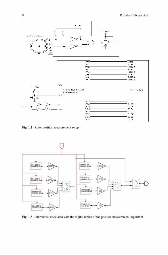
A design for measuring the rotor position is implemented. There are several compo-nents of this hardware/software design. One of them is the PepperlCFuchs encoderthat is physical attached to the motor shaft. The second one is an ATmega8535microcontroller-based signal conditioning circuit and the third one is the real timesoftware that calculates the rotor position from the digital signals provided by themicrocontroller. The ATmega8535 microcontroller is programmed for being usedas a 16-bit binary UP/DOWN counter. A signal conditioning circuit is necessary todetermine the shaft direction, which is implemented by using a flip-flop integratedcircuit. The flip-flop uses the pulses of channels A and B of the encoder and pro-vides a binary 1 or 0 depending on the shaft direction. Channel A (or B) of theencoder is then connected to a micro-controller terminal. In this case, the encodergenerates 1,024 pulses per revolution. The micro-controller count goes up or downdepending on the flip-flop binary signal. The complete electronics diagram of the ro-tor position measurement setup is shown in Fig. 1.2. The micro-controller providesa 16-bit binary count that represents the rotor position. The algorithm to interpretthe 16-bit binary count is coded in the Scilab/Scicos source program. A part of thisalgorithm is shown in Fig. 1.3. The algorithm consists of multiplying each bit (1 or0) by its corresponding value in the decimal system. Once the results are added adecimal measurement of the rotor position is obtained.
8 R. Salas-Cabrera et al.
Fig. 1.2 Rotor position measurement setup
Fig. 1.3 Subroutine associated with the digital inputs of the position measurement algorithm

1 On the Experimental Control of a Separately Excited DC Motor 9
A final super block called Position Measurement Algorithm (see Fig. 1.1) was cre-ated to include the described code. It is important to mention that the rotor positionsetup is able to measure positive and negative values. In order to accomplish thisfeature, the microcontroller was programmed to have an initial count that is locatedat the middle of the 16-bit count range.
1.3.3 Power Converter
A Pulse Width Modulation-based MOSFET H-Bridge converter was designed andimplemented. This type of power electronics device is commonly used to drive DCmotors when bidirectional speed/position control is needed. The numerical value ofthe armature voltage is defined by the state feedback and calculated by the computer.This value is written by the real time program to one of the analog output channelsof the data acquisition card. The power electronics converter and motor are shownin Fig. 1.4.
Fig. 1.4 Power converter and DC motor. (a) Signal conditioning. (b) PWM and switching delay.(c) Isolation. (d) H bridge and DC motor

10 R. Salas-Cabrera et al.
1.4 Experimental Results
This section presents the experimental transient characteristics of the closed loopsystem. The armature voltage is computed as a function of estimated states except-ing the rotor position, which is the only state variable that is measured. Estimatedstates, including the load torque, are obtained by solving the full order discrete-timestate observer in (1.10). Initial conditions of the integrator and observer state vari-ables were set numerically equal to zero. The experimental trace shown in Fig. 1.5illustrates the dynamic characteristic of the rotor position following a 25.1328radian (4 revolution) reference command. The simulated model-based trace of therotor position is also shown in Fig. 1.5. It is clear that these signals (simulated andmeasured) are similar to each other. Initially, the rotor position was at zero radians.The position begins to increase immediately until the position error is close to zero,which occurs approximately at 1.2 s. In order to save these transient data, a real-timeblock called FIFO was used [2,3]. Experimental observer-based variables were alsosaved by using FIFO. One of these variables is shown in Fig. 1.6. The armaturevoltage computed by the real time program is depicted in Fig. 1.7.
For the purpose of testing the experimental closed loop system in a more de-manding operating condition, we installed an inertial disk. The original value of theinertia was 0.0038 kg/m2, see Table 1.1. The new inertia is 0.0398 kg/m2. In otherwords, the new parameter (inertia) is about 10.5 times the original value. It meansa significant increase of a particular parameter of the mechanical subsystem. It isclearly connected to the output to be controlled (rotor position). In addition, theinertial disk was intentionally slightly loose to the shaft, therefore the parametervaried during the test around the non-original value. The original gains that werecalculated by using the nominal parameters in Table 1.1 were not changed during
-5
0
5
10
15
20
25
30
0.0 0.2 0.4 0.6 0.8 1.0 1.2 1.4 1.6 1.8Time (seconds)
Position (radians)
Fig. 1.5 Rotor position: – Experimental measured, ** Simulated model-based

1 On the Experimental Control of a Separately Excited DC Motor 11
-10
0
10
20
30
40
50
60
70
0.0 0.2 0.4 0.6 0.8 1.0 1.2 1.4 1.6 1.8Time (seconds)
Speed (rad/s)
Fig. 1.6 Rotor speed: – Experimental observer-based, ** Simulated model-based
-10
0
10
20
30
40
50
60
0.0 0.2 0.4 0.6 0.8 1.0 1.2 1.4 1.6 1.8Time (seconds)
Armature Voltage (volts)
Fig. 1.7 Armature voltage: – Experimental, ** Simulated model-based
0
5
10
15
20
25
0 2 4 6 8 10Time (seconds)
Position (radians)
Fig. 1.8 Experimental measured rotor position when a significant change of a parameter occurs(10.5 times the original value approx.)
12 R. Salas-Cabrera et al.
this test. Even under that demanding condition the experimental closed loop systemwas able to follow a 21.99 radian (3.5 revolution) reference command, see Fig. 1.8.
References
1. Boizot, N., Busvelle, E., Sachau, J.: High-gain observers and Kalman filtering in hard real-time. RTL 9th Workshop, 2007
2. Bucher, R., Mannori, S., Netter, T.: RTAI-Lab tutorial: Scilab, comedi and real-time control.http://www.rtai.org. 2008
3. Campbell, S.L., Chancellier, J.P., Nikoukhah, R.: Modeling and simulation in Scilab/Scicos.Springer, New York (2006)
4. Franklin, G.F., Powell, J.D., Workman, M.: Digital control of dynamic systems. AddisonWesley, Menlo Park, CA (1998)
5. Jugo, J.: Real-time control of a DC motor using Scilab and RTAI. Scilab INRIA Rocquen-court, 2004
6. Knoppix: Open source Linux distribution. Knoppix 5.0, 20047. Krause, P.C., Wasynczuk, O., Sudhoff, S.D.: Analysis of electrical machinery and drive sys-
tems. Wiley, IEEE Press Power Engineering (2004)8. Merry, R., van de Molengraft, R., Steinbuch, M.: Error modeling and improved position es-
timation for optical incremental encoders by means of time stamping. American ControlConference, 2007
9. National-Instruments: PCI-6024E National Instruments Manual (2006)10. Rendon-Fraga, E.Y.: Rotor position control of a DC motor using a real time platform. M.Sc.
thesis (in spanish). Instituto Tecnologico de Cd. Madero. Cd. Madero, Mexico (2009)11. Schleef, D., Hess, F., Bruyninckx, H.: The control and measurement device interface handbook.
http://www.comedi.org, 200312. Zhao, D., Zhang, N.: An improved nonlinear speed controller for series DC motors. IFAC 17th
World Congress, 2008
Chapter 2MASH Digital Delta–Sigma Modulatorwith Multi-Moduli
Tao Xu and Marissa Condon
Abstract This chapter proposes a novel design methodology for a Multi-stAgenoise SHaping (MASH) digital delta–sigma modulator (DDSM) which employsmulti-moduli. The structure is termed the MM-MASH. The adequacy and benefit ofusing such a structure is demonstrated. In particular, the sequence length is length-ened if the quantizer modulus of the first-order error feedback modulator (EFM1)of each stage are co-prime numbers. An expression for the sequence length of anMM-MASH is derived.
Keywords Delta–sigma modulation � sequence length � multi-moduli � co-primenumbers
2.1 Introduction
The digital delta–sigma modulator (DDSM) sometimes acts as the controller ofthe multi-modulus frequency divider in the feedback loop of the Fractional-NFrequency Synthesizers [4]. Since the DDSM is a finite state machine, when theinput is a DC rational constant, the output is always a repeating pattern (limitcycle) [2, 8]. The period of the cycle is termed the sequence length. For this type ofinput, the quantization noise is periodic. When a sequence length is short, the poweris distributed among spurious spurs that appear in the DDSM output spectrum.Hence, there is a desire to break short sequences. Dithering [10, 11] is one of themost commonly employed methods to break the short sequence length. However, itrequires extra hardware and inherently introduces additional inband noise. Recently,
T. Xu (�) and M. CondonRF Modelling and Simulation Group, Research Institute for Networks and CommunicationsEngineering (RINCE), School of Electronic Engineering, Dublin City University,Glasnevin, Dublin 9, Irelande-mail: [email protected]; [email protected]
S.-I. Ao and L. Gelman (eds.), Electronic Engineering and Computing Technology,Lecture Notes in Electrical Engineering 60, DOI 10.1007/978-90-481-8776-8 2,c� Springer Science+Business Media B.V. 2010
13

14 T. Xu and M. Condon
some design methodologies have been proposed to maximise the sequence length.Borkowski [2] summarises the maximum period obtained by setting the initial con-dition of the registers in an EFM. Hosseini [7] introduced a digital delta–sigmamodulator structure termed the HK-MASH with a very long sequence. The periodof the HK-MASH is proven by mathematical analysis [6, 7]. This paper proposes anovel architecture to further increase the modulator sequence length.
This chapter proposes that the modulus of each quantizer in a DDSM is set asa different value from each other. Note that each quantizer has only one modulus.Furthermore, all of the moduli are co-prime numbers. Co-prime numbers [3] aretwo real numbers whose greatest common divisor is 1. They do NOT have to beprime numbers. A novel design methodology based on this concept is proposed. Itwill be shown to increase the modulator period and consequently reduce the effectof quantization noise on the useful output frequency spectrum of the DDSM.
In Section 2.2, the architectures of the classic MASH DDSM and the HK-MASHare reviewed. In Section 2.3, a novel structure is proposed that results in the max-imum sequence length. The expression for the sequence length is derived as well.The simulation results are shown in Section 2.5.
2.2 Previous MASH Architectures
The architecture of an l th order MASH digital delta–sigma modulator (DDSM) isillustrated in Fig. 2.1. It contains l first-order error-feedback modulators (EFM1).xŒn� and yŒn� are an n0-bit input digital word and anm-bit output, respectively. Therelationship between them is
mean.y/ D X
M(2.1)
where X is the decimal number corresponding to the digital sequence xŒn� [1], i.e.,xŒn� D X 2 f1; 2; : : : ;M g, and M is the quantizer modulus which is set as 2n0 inthe conventional DDSM.
Fig. 2.1 MASH DDSM architecture

2 MASH Digital Delta–Sigma Modulator with Multi-Moduli 15
Fig. 2.2 EFM1: first-ordererror-feedback modulator
Fig. 2.3 The modified EFM1used in HK-MASH
The model of the EFM1 is shown in Fig. 2.2. This is a core component in themake-up of the MASH digital delta–sigma modulator (DDSM). The rectangleZ�1
represents the register which stores the error eŒn� and delays it for one time sample.Q.�/ is the quantization function:
yŒn� D Q.uŒn�/ D�1; uŒn� �M0; uŒn� < M
(2.2)
where
uŒn� D xŒn�C eŒn � 1�: (2.3)
The maximum sequence lengths for this structure are 2n0C1 or 2n0C2 when themodulator order is below 5, which is found from simulations [2]. To achieve bothof these sequence lengths, the first stage EFM1 must have an odd initial condition.This is implemented by setting the register.
The architecture of the modified EFM1 used in the HK-MASH is illustrated inFig. 2.3. The only difference between it and the conventional EFM1 in Fig. 2.2 isthe presence of the feedback block aZ�1. a is a specifically-chosen small integerto make (M � a) the maximum prime number below 2n0 [7]. The sequence lengthof it is .2n0 � a/l � .2n0/l . This value will be compared with that of the proposednovel MM-MASH in Section 2.4.
2.3 The Adequacy and Effect of the Multi-ModulusMASH-DDSM
We assume that the quantizer modulus of the i th stage EFM1 in an l th order MASH-DDSM is represented byMi , where i 2 f1; 2; : : : ; lg. It shall first be shown that theMM-MASH is an accurate modulator. Then the effect of the multi-moduli on thesequence length shall be investigated mathematically.

16 T. Xu and M. Condon
2.3.1 The Suitability of the Multi-Modulus MASH-DDSM
In a fractional-N frequency synthesizer, the static frequency divider is controlledby the average value of the delta–sigma modulator output, mean.y/. The goal is toshow that in an MM-MASH, mean.y/ is affected only by the quantizer modulus ofthe first stage EFM1,M1, and is independent of the moduli in other stages. With thisbeing true, having a multi-modulus architecture does not affect the accuracy of thedigital delta–sigma modulator. Hence, it is a suitable digital delta–sigma modulator.Required to prove:
mean.y/ D X
M1
: (2.4)
Proof. As seen in Fig. 2.1, at the output of the last adder,
vl�1Œ1� D yl�1Œ1�C yl Œ1� � yl Œ0� (2.5)
vl�1Œ2� D yl�1Œ2�C yl Œ2� � yl Œ1� (2.6)
:::
vl�1ŒN � D yl�1ŒN �C yl ŒN � � yl ŒN � 1� (2.7)
where N is assumed as the sequence length of the MASH delta–sigma modulator.Adding all of the above equations yields:
NXkD1
vl�1Œk� DNX
kD1
yl�1Œk�CNX
kD1
yl Œk� �N�1XkD0
yl Œk� (2.8)
where the period of yl is assumed as Nl . As seen in Fig. 2.1, the output of theMASH modulator is obtained by simply summing and/or subtracting the output ofeach EFM1. Hence, the period of the MASH DDSM is the least common multipleof the sequence length of each stage. In other words, N is a multiple of Ni , whereNi is the period of the i th stage EFM1 and i 2 f1; 2; : : : ; lg. It follows that
NXkD1
yl Œk� DN�1XkD0
yl Œk�: (2.9)
Thus (2.8) becomes:
NXkD1
vl�1Œk� DNX
kD1
yl�1Œk�: (2.10)
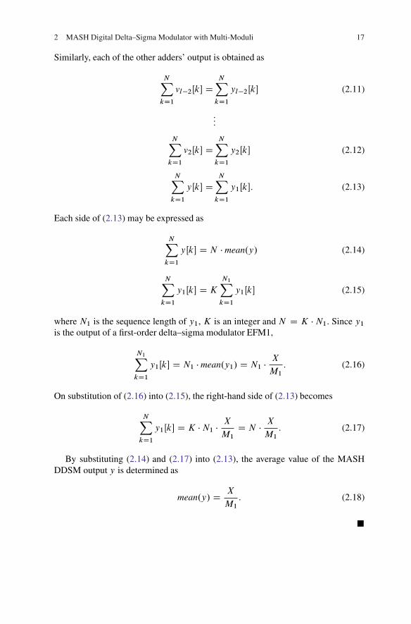
2 MASH Digital Delta–Sigma Modulator with Multi-Moduli 17
Similarly, each of the other adders’ output is obtained as
NXkD1
vl�2Œk� DNX
kD1
yl�2Œk� (2.11)
:::
NXkD1
v2Œk� DNX
kD1
y2Œk� (2.12)
NXkD1
yŒk� DNX
kD1
y1Œk�: (2.13)
Each side of (2.13) may be expressed as
NXkD1
yŒk� D N � mean.y/ (2.14)
NXkD1
y1Œk� D KN1X
kD1
y1Œk� (2.15)
where N1 is the sequence length of y1, K is an integer and N D K � N1. Since y1
is the output of a first-order delta–sigma modulator EFM1,
N1XkD1
y1Œk� D N1 � mean.y1/ D N1 � XM1
: (2.16)
On substitution of (2.16) into (2.15), the right-hand side of (2.13) becomes
NXkD1
y1Œk� D K �N1 � XM1
D N � XM1
: (2.17)
By substituting (2.14) and (2.17) into (2.13), the average value of the MASHDDSM output y is determined as
mean.y/ D X
M1
: (2.18)
�

18 T. Xu and M. Condon
2.3.2 The Effect of the Multi-Moduli on the ModulatorSequence Length
It is required to prove that the sequence length of the MASH modulator dependson the product of all the quantizer moduli. The expression for the l th order MASHDDSM sequence length is
N D M1 �M2 � : : : �Ml
�(2.19)
where � is a parameter to makeN the least common multiple of the sequence lengthof each stage Ni .
In addition, if the following two conditions, C1 and C2, are satisfied:
1. X and M1 are co-prime numbers2. fM1, M2, . . . , Mlg are co-prime numbers
then the sequence length of the MASH DDSM attains the maximum value:
Nmax DM1 �M2 � : : : �Ml : (2.20)
Proof : In the first-stage EFM1 shown in Fig. 2.2,
e1Œ1� D uŒ1� � y1Œ1�M1
D X C e1Œ0� � y1Œ1�M1 (2.21)
e1Œ2� D X C e1Œ1� � y1Œ2�M1 (2.22)
:::
e1ŒN1� D X C e1ŒN1 � 1�� y1ŒN1�M1 (2.23)
where e1Œ0� is the initial condition of the register. The sum of all of the aboveequations is
N1XkD1
e1Œk� D N1XCN1�1XkD0
e1Œk� �N1X
kD1
y1Œk�M1: (2.24)
Since in the steady state, the first EFM1 is periodic with a period N1 [5],
N1XkD1
e1Œk� DN1�1XkD0
e1Œk�: (2.25)
Hence, (2.24) may be modified to
N1XkD1
y1Œk� D N1X
M1
: (2.26)