Seismological Research Letters Volume 83, Number 2 March/April 2012 281doi: 10.1785/gssrl.83.2.281

Listen, Watch, Learn: SeisSound Video Products

Debi Kilb,1 Zhigang Peng,2 David Simpson,3 Andrew Michael,4 Meghan Fisher,5 and Daniel Rohrlick1

INTRODUCTION TO SEISSOUND VIDEO PRODUCTS

format of how information is distributed and assimilated, high-lighting the importance of including auditory information in videos. Videos that include sound also permeate the research community, as evidenced by their recent increase within online supplements to journal articles. Tapping into this new approach

that augment visual imagery with auditory counterparts. We term these “SeisSound” video products (Figure 1). We !nd the

appreciated using these SeisSound products than using just the individual visual or the auditory components independently.

Seismology includes the study of a large number of pro-cesses that a"ect the spectral content of a seismogram including

and the di"erences between abrupt tectonic earthquakes and unusual sources such as volcanic and non-volcanic tremor. With training, we can learn to discern the seismic signatures of these di"erent processes, which can be inferred from the

however, subtle di"erences in these signals can be di#cult to

A number of our senses include the ability to act as spec-tral analyzers. In the audible sound range we hear pitch, in the visible light range we see color, and in the low- and sub-audi-ble range we can feel the di"erence between sudden and slow

motions using our senses of motion and touch. For most peo-ple, the concepts of high or low pitch (frequency) and volume (amplitude) are innate. When we listen to a symphony orches-tra, we can pick out the sound of individual instruments and decipher the unique spectral content of their tones even though a hundred musicians are playing simultaneously. Similarly, we can teach people how to use these innate abilities to under-stand seismology by having them listen to the frequency con-

the auditory can increase the connection between the heard pitch and the visually observed frequency content within

paper Peng et al. 2012, this issue, in the EduQuakes column).

ability to communicate e"ectively with diverse audiences who have a variety of learning styles and levels.

$e audible frequency range for humans is roughly 20

(or seven to ten octaves) higher than the frequency content for most recorded earthquake signals. To bring the sub-audible frequency content of earthquake seismograms into the audible range, the seismic data need to be shi%ed to a higher pitch. To accomplish this, the simplest and purest method is to time compress the seismogram (Dombois and Eckel 2011) by increasing the playback speed rel-ative to the recording rate. Time compression also allows us to play back a long record in a reasonable amount of time during a lecture or demonstration.

Time compression as a method to convert seismic data to

of the general !eld of “soni!cation,” which can involve more

various sound attributes ( pitch, volume, and timbre). Early

advent of magnetic tape recording, which allowed playback at speeds higher than the recorded speed. One of the earliest

and teleseismic earthquakes recorded on an early tape sys-

using magnetic tape recording also was tested successfully as a

recording tape system to record a variety of earthquakes and

processing in their analysis. Some of these events were used as part of the “Murmurs of Earth” collection for the “Interstellar

1. Institute of Geophysics and Planetary Physics, University of

2. School of Earth and Atmospheric Sciences, Georgia Institute of Technology, Atlanta, Georgia

Electronic SeismologistDebi Kilb et al.

S E I S M O L O G I S T

E L E C T R O N I C

282 Seismological Research Letters Volume 83, Number 2 March/April 2012

(Sagan et al.recording in seismology, it is now possible to convert seismic waveforms to standard audio formats and apply simple !lter-ing and time-compression techniques using widely available audio processing so%ware. $ese types of auditory presenta-tions of seismic data are now commonly used for educational purposes (and have recently regained popularity to highlight di"erences between typical earthquake recordings and tremor-like signals (Simpson et al. et al. 2010).

METHOD

Overview $e SeisSound visual component includes the seismogram and corresponding spectrogram, presented in movie format indi-cating how the data evolve with time. An auditory sound !le

(WAVE format) of the data that are time compressed accom-panies the visual information so the frequency content of the

-ties in the frequency-time distribution of the seismogram that are o%en otherwise hidden in large-amplitude signals. $ese SeisSound video products provide a unique way to watch and listen to the vibration of the Earth, and help introduce more advanced topics in seismology.

Our computer codes are written with MATLAB and are freely available for use (see the electronic supplement’s MATLAB codes and data bundle). $ese MATLAB codes produce an audio !le and a sequence of static image !les. $e audio track is produced using the MATLAB function -

, which allows a scaling factor to be applied to speed up or slow down the playback speed. It typically takes only a few min-utes for the code to process a standard seismogram. A bundled !le that contains the MATLAB programs and sample data is

!"

!#

0

#

"

x 106

#$$#%&'()*%+,-./0%1.23456.7,8%93.30:-%;<=>+&%;??,/,2.30:-%

962@.?,%A.B,

!"$$

!#$$

0

#$$

"$$ C.-D!E.FF%#!*%GH

I0J,%KFL8%"$$%30J,F%@.F3,2%34.-%326,%FM,,D

N2,56,-?O%KGHL

#$$ "$$ 600 *$$ 1000 P#$$ P"$$ 1600 P*$$0

5

10

15

!Q$

!"$

!R$

!#$

!P$

9M,?32:S2.J

! Figure 1. Snapshot from a sample SeisSound video product. Shown is the transverse component of data from the 2002 magnitude 7.8 Denali earthquake in Alaska, recorded at station RDM in southern California (distance of ~4,000 km). The seismogram trace changes from light to dark as a time indicator progression line (vertical pink line) moves from left to right in the video. Original data (top). Data bandpass filtered 2–8 Hz. (middle). Spectrogram (bottom). Note the locally triggered tremors at 1,000–1,400 s that correspond to the arrival of the large amplitude surface waves (Gomberg et al. 2008; Chao et al. 2012). To remove any high-frequency artifacts introduced from using a short time window of data, we applied a 0.5 Hz high-pass filter to the data before computing the spectrogram (Peng et al. 2011).

Seismological Research Letters Volume 83, Number 2 March/April 2012 283

available from our electronic supplement (MATLAB codes and data bundle). Figure 2 shows the recommended directory structure for the codes and data. A list of the MATLAB pro-grams and a description of the parameters used to call the main program are listed in Tables 1 and 2.

For each seismogram, the MATLAB code reads seismic et

al.-

tion of the seismogram and spectrogram data with time. We use the so%ware QuickTimePro to concatenate the images into a video and add the corresponding audio !le in sync with the video to create a SeisSound video. $e !nal SeisSound video

and size of the images and the total number of frames in the video. In addition to the video product, we also include a stand-alone MATLAB code sac2wav.m to directly convert seismic

Research Institutions for Seismology (IRIS) Data Management -

forms from the archive and converting them to WAVE format (http://www.iris.edu/ws/timeseries/).

Steps Required to Create SeisSound Products$ere are two main steps required to create a SeisSound video. $e !rst step requires running the SeisSound.m MATLAB code to produce an audio WAVE !le and the sequence of images. As the code runs, it will display images of the data in three panels. $e top panel shows the original seismogram, the middle panel a !ltered version of the data, and the bottom a spectrogram of the data ( see Figure 1). If you encounter an error message indicating a missing variable or function, check that you have all of the required routines (see Table 1) and that the codes and data are stored in the proper location in the directory structure (Figure 2). If the code runs success-fully, a noti!cation of “Render Finished” will be issued at the MATLAB command window and two new subdirectories named “Audio” and “Images” will be added appropriately ( see Figure 2). In the second step, the audio and image !les are

It is relatively straightforward to process seismic wave-

(http://www.iris.edu/ws/timeseries) can be used to preprocess ( !l-ter and scale) the data. Station and waveform metadata ( station code, start time, sample rate, etc.) are transferred to the

-mation required to create the SeisSound products is provided via parameters in the calling function as described in Table 2.

SAMPLE SEISSOUND VIDEO PRODUCTS

di"erences in the frequency and temporal characteristics of dif-ferent seismic signals, can be found in our electronic supplement. Because of the wide dynamic range, the sound can be better appreciated on a computer with good speakers or with earbuds to hear the full e"ect of the lower frequencies. $e amplitude of the low frequencies can sometimes be large, so it is best to keep the volume initially low to avoid damaging the speakers or, if you are using earbuds, your ears. With these SeisSound prod-ucts, students can begin to decipher and understand compli-cated earthquake physics and earthquake triggering processes.

Notable signatures in the videos can be indicative of certain

the spectrogram, corresponding to popping sounds that begin at a fast rate and then ebb (

AFI_aftershock_movie60FPS.mov) are characteristic of a main-shock/a%ershock sequence ( Peng et al. et al. -trogram accompanied by a repetitive pop-pop-pop tempo sound (

MtStHelen_Drumbeat.mov) is a characteristic of “drum beat” earthquake swarms during volcanic eruptions (Iverson et al. 2006). Another similar, yet distinctly di"erent, signature is that of triggered deep non-volcanic tremor that

Base Directory

Images Audio

Data_A Data_B

Images Audio

Data_C

Images Audio

CODES

! Figure 2. Suggested directory structure. The “Images” and “Audio” subdirectories will be automatically added and filled by the SeisSound.m MATLAB program.

TABLE 1Description of MATLAB routines used to create the

sound and image files for SeisSound video products. The electronic supplement MATLAB codes and data bundle

contains a bundle of these codes and sample data.

Filename Purposeeqfiltfilt.m perform a Butterworth filterfget_sac.m read sac formatted data into MATLAB linex.m draw a vertical line at a specified position main_tremor.m main program that calls SeisSoundsac.m read a single SAC data file sachdr.m read the header file of SAC formatted dataSeisSound.m [Main program] generated images and an

audio wave filesac2wav.m create an audio wave file from SAC

formatted data

284 Seismological Research Letters Volume 83, Number 2 March/April 2012

typically occurs during the passage of the surface waves ( Peng et al.the spectrogram during the surface wave portion of the seismic wavetrain accompanied by a relatively short-lived rat-a-tat-tat sound as from a snare drum ( Triggered tremor in Park!eld,

Denali_Triggered_Tremor.movthe electronic supplement bundled !le are set up to create this

AUDIENCE AND USES FOR SEISSOUND VIDEO PRODUCTS

-tings and public lectures ranging from teaching kindergarten-ers to educating more advanced audiences, including graduate

and sounds immediately captivate audiences regardless of their

adjusted for each group. $e innovative combination of audi-tory and visual information is particularly useful for introduc-

ing seismic data to beginning researchers, including upper-level undergraduate and !rst-year graduate students in introductory geophysics or seismology courses.

SeisSound videos can be used to highlight di"erences in the amplitude, frequency, and duration of P and S and sur-face waves and to teach how to discriminate between seismic signatures of teleseismic and local earthquakes. For the more

can be more easily discussed and investigated by incorporat-ing sound include: categorizing seismic wave attenuation with distance from the source, discriminating between large and small earthquakes, identifying a%ershock rates, and recogniz-ing site e"ects including reverberation in basins ( Benio"

et al. et al. 2010). SeisSound products can also be useful in discriminating com-plicated seismic signals from multiple sources, such as a%er-shocks within the coda of large earthquakes ( Peng et al.

et al.(Hill et al. Peng et al.

TABLE 2Parameters required to call the SeisSound.m MATLAB function. The number in column 1 indicates the position of this

parameter in the function call list. The formal function call uses this format: function SeisSound(inputdata, directory, titleit, starttime, endtime, filt_low, filt_high, ff_max, units, dtype, speed_factor, ColorBar_Upper_Limit, ColorBar_Lower_Limit,

FramesPerSecond). An example of how to call the program can be found in “main_tremor.m.”

Parameter Name Description Default1 inputdata Data file name BK.PKD.HHT.SAC2 directory Name of the folder where the data resides and where the

code generated images and audio directories will be addedDenali_2002_at_Parkfield

3 titleit Title to be used on all generated images Data from [name of input data file] 4 starttime Seismogram start time in seconds, use -999 to use the start

time of the data–999

5 endtime Seismogram end time in seconds, use -999 to use the end time of the data

–999

6 filt_low Lower band limit if data filtering is requested (for low-pass only or no filter use -999)

–999

7 filt_high High band limit if data filtering is requested (for high-pass only or no filter use -999)

–999

8 ff_max Enforced maximum frequency for the spectrogram (use -999 to display all available frequencies)

–999

9 units Units for seismogram y-axis label (e.g., cm/s or cm/s/s). Use -999 to display no units.

–999

10 dtype Data type (e.g., displacement, velocity, or acceleration). Use -999 to default to data type specified in the SAC file (i.e., hdr.descrip.idep).

–999

11 speed_factor Audio file scale factor 10012 ColorBar_Upper_Limit Upper limit of the color bar of the spectrogram 013 ColorBar_Lower_Limit Lower limit of the color bar of the spectrogram –8014 FramesPerSecond The frame per second rate you plan to use in your final

SeisSound movie; this parameter will determine the number of images generated. Use -999 to let the program select the rate for you.

–999

Seismological Research Letters Volume 83, Number 2 March/April 2012 285

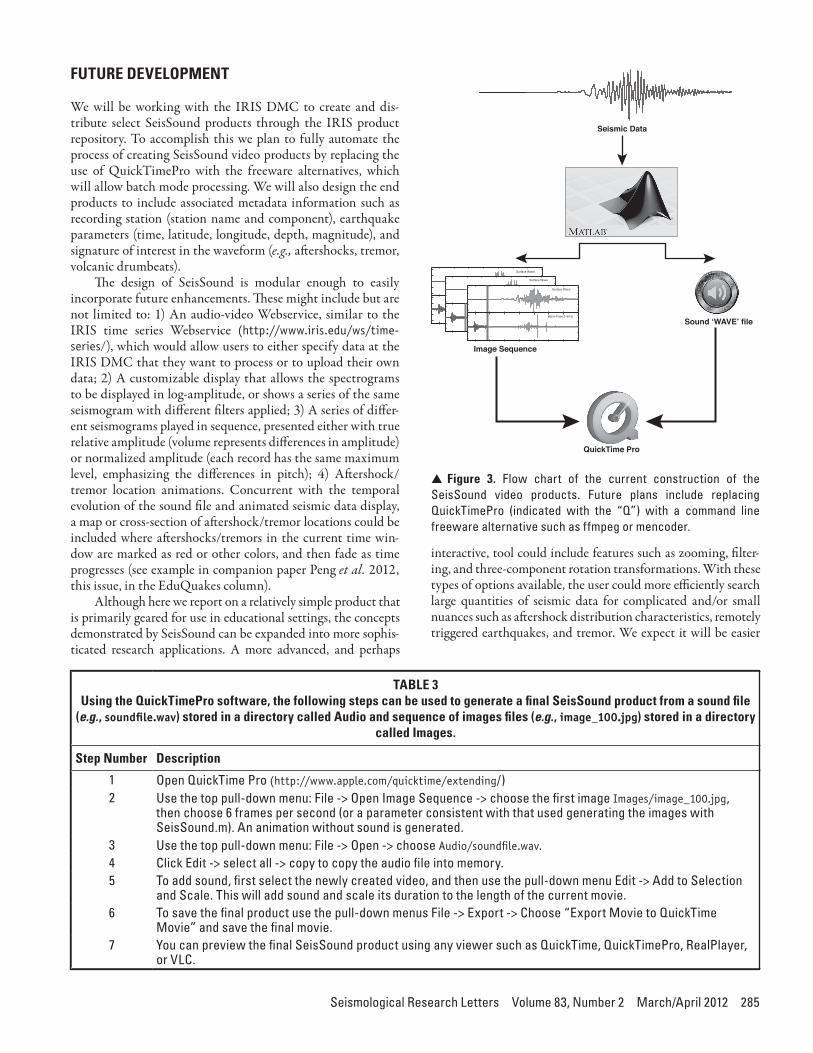
FUTURE DEVELOPMENT

-tribute select SeisSound products through the IRIS product repository. To accomplish this we plan to fully automate the process of creating SeisSound video products by replacing the use of QuickTimePro with the freeware alternatives, which will allow batch mode processing. We will also design the end products to include associated metadata information such as recording station (station name and component), earthquake parameters (time, latitude, longitude, depth, magnitude), and signature of interest in the waveform ( a%ershocks, tremor, volcanic drumbeats).

$e design of SeisSound is modular enough to easily incorporate future enhancements. $ese might include but are not limited to: 1) An audio-video Webservice, similar to the IRIS time series Webservice (http://www.iris.edu/ws/time-series/), which would allow users to either specify data at the

to be displayed in log-amplitude, or shows a series of the same -

ent seismograms played in sequence, presented either with true relative amplitude (volume represents di"erences in amplitude)

evolution of the sound !le and animated seismic data display, a map or cross-section of a%ershock/tremor locations could be included where a%ershocks/tremors in the current time win-dow are marked as red or other colors, and then fade as time

et al. 2012, this issue, in the EduQuakes column).

Although here we report on a relatively simple product that is primarily geared for use in educational settings, the concepts

-ticated research applications. A more advanced, and perhaps

interactive, tool could include features such as zooming, !lter-ing, and three-component rotation transformations. With these types of options available, the user could more e#ciently search large quantities of seismic data for complicated and/or small nuances such as a%ershock distribution characteristics, remotely

Image Sequence

Sound !WAVE" file

QuickTime Pro

Seismic Data

Surface Wave

C.-D!E.FF%#!*%GH

Surface Wave

C.-D!E.FF%#!*%GH

Surface Wave

C.-D!E.FF%#!*%GH

! Figure 3. Flow chart of the current construction of the SeisSound video products. Future plans include replacing QuickTimePro (indicated with the “Q”) with a command line freeware alternative such as ffmpeg or mencoder.

TABLE 3Using the QuickTimePro software, the following steps can be used to generate a final SeisSound product from a sound file

(e.g., soundfile.wav) stored in a directory called Audio and sequence of images files (e.g., image_100.jpg) stored in a directory called Images.

Step Number Description

1 Open QuickTime Pro (http://www.apple.com/quicktime/extending/)2 Use the top pull-down menu: File -> Open Image Sequence -> choose the first image Images/image_100.jpg,

then choose 6 frames per second (or a parameter consistent with that used generating the images with SeisSound.m). An animation without sound is generated.

3 Use the top pull-down menu: File -> Open -> choose Audio/soundfile.wav.4 Click Edit -> select all -> copy to copy the audio file into memory.5 To add sound, first select the newly created video, and then use the pull-down menu Edit -> Add to Selection

and Scale. This will add sound and scale its duration to the length of the current movie.6 To save the final product use the pull-down menus File -> Export -> Choose “Export Movie to QuickTime

Movie” and save the final movie.7 You can preview the final SeisSound product using any viewer such as QuickTime, QuickTimePro, RealPlayer,

or VLC.

286 Seismological Research Letters Volume 83, Number 2 March/April 2012

to detect these key features using combined audio/visual tech-niques than with traditional or automated processing.

ACKNOWLEDGMENTS

We thank an anonymous reviewer and SRL Associate Editor John N. Louie for their help and guidance. Integral to the success of this project was our participation in the Southern

-nered undergraduate student MF in ZP’s lab in the summer of

Support for this work included funding from IRIS sub-award -

AM grew out of the online seminar series “Teaching Geophysics

and Research,” which was part of the “Professional Development for Geoscience Faculty” project.

REFERENCES

-Bulletin of the Seismological Society of

America 102 Dombois, F. (2001). Listen to seismograms: About acoustic interpreta-

tion of seismometric records. Geophysical Research Abstracts 3Dombois, F., and G. Eckel (2011). Audi!cation. In !e Soni"cation

HandbookBerlin: Logos Publishing House http://sonification.de/handbook/index.php/chapters/chapter12/.

Fisher, M., Z. Peng, D. W. Simpson, and D. L. Kilb (2010). Hear it, see

, Fall Meeting

Bulletin of the Seismological Society of America 55

Signal processing&and analysis tools for seismologists and engineers.

SeismologyKisslinger. Amsterdam & Boston: Academic Press.

community. Incorporated Institutions for Seismology Data https://e-reports-ext.

llnl.gov/pdf/318698.pdf.

Science 319 10.1126/scienceAuditory Display:

, ed. G. Kramer,

Hill, D. P., P. A. Reasenberg, A. J. Michael, W. J.. Arabasz, G. Beroza, D. Brumbaugh, J. N. Brune, et al.

Science 260

LaHusen, M. Lisowski, J. J. Major, S. D. Malone, J. A. Messerich,

Nature 444 10.1038/nature

thresholds as a function of time: Results from the ANZA seismic ML

earthquake. Bulletin of the Seismological Society of America 97,

http://earth-quake.usgs.gov/learn/listen/index.php.

Michael, A. J. (2011). Earthquake sounds. In Encyclopedia of Solid Earth Geophysics

-mic station. Bulletin of the Seismological Society of America 62,

to the 2011 magnitude 9.0 Tohoku-Oki, Japan, earthquake. Seismological Research Letters 83

Peng, Z., L. T. Long, and P. Zhao (2011). $e relevance of high-frequency analysis artifacts to remote triggering. Seismological Research Letters 82 10.1785/gssrl

2002 Denali fault earthquake. Geophysical Research Letters 35,

Peng, Z., J. E. Vidale, and H. Houston (2006). Anomalous early a%er-M 6 Park!eld earthquake. Geophysical

Research Letters 33

rate immediately before and a%er main shock rupture from high-frequency waveforms in Japan. Journal of Geophysical Research 112,

Remote triggering of tremor along the San Andreas fault in cen-Journal of Geophysical Research 114

. New

Earth. Seismological Research Letters 76Simpson, D. W., Z. Peng, D. Kilb, and D. Rohrick (2009). Soni!cation

of earthquake data: From wiggles to pops, booms and rumbles.

Speeth, S. D. (1961). Seismometer sounds. Journal of the Acoustical Society of America 33

Scripps Institution of OceanographyUniversity of California at San Diego

IGPP 0225La Jolla, California 92093-0225 U.S.A.

dkilb@epicenter.ucsd.edu(D. K.)