electron transport, interaction and spin in graphene and - diva
TRANSCRIPT

Linköping Studies in Science and TechnologyDissertation No. 1469
Electron transport, interaction and spin ingraphene and graphene nanoribbons
Artsem Shylau
Department of Science and TechnologyLinköping University, SE-601 74 Norrköping, Sweden
Norrköping 2012
Cover illustration: zigzag graphene nanoribbon attached to leads
Electron transport, interaction and spin in graphene and graphene nanoribbons
© 2012 Artsem Shylau
Department of Science and TechnologyLinköping University, SE-601 74 Norrköping, Sweden
ISBN 978-91-7519-816-3 ISSN 0345-7524
Printed by LiU-Tryck, Linköping 2012

To my parents, Valentina and Alexander.


Abstract
Since the isolation of graphene in 2004, this novel material has becomethe major object of modern condensed matter physics. Despite of enor-mous research activity in this field, there are still a number of fundamentalphenomena that remain unexplained and challenge researchers for furtherinvestigations. Moreover, due to its unique electronic properties, grapheneis considered as a promising candidate for future nanoelectronics. Besidesexperimental and technological issues, utilizing graphene as a fundamentalblock of electronic devices requires development of new theoretical meth-ods for going deep into understanding of current propagation in grapheneconstrictions.
This thesis is devoted to the investigation of the effects of electron-electron interactions, spin and different types of disorder on electronic andtransport properties of graphene and graphene nanoribbons.
In paper I we develop an analytical theory for the gate electrostaticsof graphene nanoribbons (GNRs). We calculate the classical and quan-tum capacitance of the GNRs and compare the results with the exact self-consistent numerical model which is based on the tight-binding p-orbitalHamiltonian within the Hartree approximation. It is shown that electron-electron interaction leads to significant modification of the band structureand accumulation of charges near the boundaries of the GNRs.
It’s well known that in two-dimensional (2D) bilayer graphene a bandgap can be opened by applying a potential difference to its layers. Calcula-tions based on the one-electron model with the Dirac Hamiltonian predicta linear dependence of the energy gap on the potential difference. In paper
II we calculate the energy gap in the gated bilayer graphene nanoribbons(bGNRs) taking into account the effect of electron-electron interaction. Incontrast to the 2D bilayer systems the energy gap in the bGNRs dependsnon-linearly on the applied gate voltage. Moreover, at some intermediategate voltages the energy gap can collapse which is explained by the strongmodification of energy spectrum caused by the electron-electron interac-tions.
Paper III reports on conductance quantization in grapehene nanorib-bons subjected to a perpendicular magnetic field. We adopt the recursiveGreen’s function technique to calculate the transmission coefficient which

iv
is then used to compute the conductance according to the Landauer ap-proach. We find that the conductance quantization is suppressed in themagnetic field. This unexpected behavior results from the interaction-induced modification of the band structure which leads to formation ofthe compressible strips in the middle of GNRs. We show the existence ofthe counter-propagating states at the same half of the GNRs. The over-lap between these states is significant and can lead to the enhancement ofbackscattering in realistic (i.e. disordered) GNRs.
Magnetotransport in GNRs in the presence of different types of disorderis studied in paper IV. In the regime of the lowest Landau level thereare spin polarized states at the Fermi level which propagate in differentdirections at the same edge. We show that electron interaction leads tothe pinning of the Fermi level to the lowest Landau level and subsequentformation of the compressible strips in the middle of the nanoribbon. Thestates which populate the compressible strips are not spatially localizedin contrast to the edge states. They are manifested through the increaseof the conductance in the case of the ideal GNRs. However due to theirspatial extension these states are very sensitive to different types of disorderand do not significantly contribute to conductance of realistic samples withdisorder. In contrast, the edges states are found to be very robust to thedisorder. Our calculations show that the edge states can not be easilysuppressed and survive even in the case of strong spin-flip scattering.
In paper V we study the effect of spatially correlated distribution of im-purities on conductivity in 2D graphene sheets. Both short- and long-rangeimpurities are considered. The bulk conductivity is calculated making useof the time-dependent real-space Kubo-Greenwood formalism which allowsus to deal with systems consisting of several millions of carbon atoms. Ourfindings show that correlations in impurities distribution do not signifi-cantly influence the conductivity in contrast to the predictions based onthe Boltzman equation within the first Born approximation.
In paper VI we investigate spin-splitting in graphene in the presence ofcharged impurities in the substrate and calculate the effective g-factor. Weperform self-consistent Thomas-Fermi calculations where the spin effectsare included within the Hubbard approximation and show that the effectiveg-factor in graphene is enhanced in comparison to its one-electron (non-interacting) value. Our findings are in agreement to the recent experimentalobservations.
Popularvetenskaplig
sammanfattning
Anda sedan isoleringen av grafen ar 2004, har detta nya material blivitden viktigaste foremalet for den moderna kondenserade materiens fysik.Trots enorm forskning inom detta omrade finns det fortfarande ett an-tal grundlaggande fenomen som forblir oforklarade och utmanar forskarefor vidare undersokningar. Dessutom, pa grund av dess unika elektron-iska egenskaper, anses grafen vara en lovande kandidat for framtida na-noelektronik. Forutom experimentella och teknologiska fragor, kan grafenanvandas som ett grundlaggande block av elektroniska komponenter somkraver utveckling av nya teoretiska metoder for att fordjupa forstaelsen avstrom utbredning i nanostrukturer av grafen.
Denna avhandling tillagnar at utredningen av effekterna av elektron-elektron vaxelverkan, spin och olika typer av oordning inom elektroniskaoch transport egenskaper hos grafen och grafen nanoremsor.

vi

Acknowledgments
Despite of my primary background in applied sciences I always wished tobe a theoretical physicist, because I was always impressed by the fact thathuman mind is able to unravel Nature secrets just with the use of a pieceof paper and a pencil (or a computer nowadays). This dream got fulfilledin Sweden where I spent four years as a PhD student at ITN LiU doing myresearch in theoretical physics. Tack, Sverige!
I would like to thank a lot of people who surrounded me during thisperiod.
First of all, I would like to thank Prof. Igor Zozoulenko for his greatsupervision, significant contribution to my scientific development and formotivation when it was really needed.
I am thankful to the research administrator Ann-Christin Noren andElisabeth Andersson for their administrative help during my research work.
I had a fruitful collaboration with my colleagues from Germany, Dr.Hengyi Xu and Prof. Thomas Heinzel, and my polish colleague Dr. Jaros lawK los.
Besides the science there were a lot of other things happening in my life.I met a lot of nice people here, some of them eventually became my friends.First of all, I am grateful to Olga Bubnova for our inspiring philosophicaldiscussions, pleasant lunch time and just for being a good friend. I amalso thankful to Loıg, Anton, Brice, Sergei, Julia and especially Taras fora good company and funny talks.
All this time I kept in touch with my belarusian friends, Sergei andAlex. We had a good time together whenever I went home, to my lovelyMinsk.
Finally, I would like to thank my wife Marina for her love, understandingand patience; my parents and my sister’s family for their love and supportwhich I feel every day no matter where I am.
Artsem ShylauNorrkoping, August 2012

viii

List of publications
Publications included in the thesis
1. A. A. Shylau, J. W. Klos, and I. V. Zozoulenko, Capacitance ofgraphene nanoribbons, Phys. Rev. B 80, 205402 (2009).
Author’s contribution: Implementation of the self-consistent nu-merical model and all numerical calculations, partial contribution todevelopment of the analytical model. Preparation of all the figures.Initial draft of the paper.
2. Hengyi Xu, T. Heinzel, A. A. Shylau, I. V. Zozoulenko, Interactionsand screening in gated bilayer graphene nanoribbons, Phys. Rev. B82, 115311 (2010); selected as ”Editor’s Suggestion”.
Author’s contribution: Development of the analytical model. Dis-cussion and analysis of all the obtained results.
3. A. A. Shylau, I. V. Zozoulenko, Hengyi Xu, T. Heinzel, Genericsuppression of conductance quantization of interacting electrons ingraphene nanoribbons in a perpendicular magnetic field, Phys. Rev.B 82, 121410(R) (2010).
Author’s contribution: All numerical calculations and preparationof all the figures. Discussion of the results and writing an initial draft.
4. A. A. Shylau and I. V. Zozoulenko, Interacting electrons in graphenenanoribbons in the lowest Landau level, Phys. Rev. B 84, 075407(2011).
Author’s contribution: All numerical calculations and preparationof all the figures, discussion of the results and writing an initial draft.
5. T. M. Radchenko, A. A. Shylau, and I. V. Zozoulenko, Influenceof correlated impurities on conductivity of graphene sheets: Time-dependent real-space Kubo approach, Phys. Rev. B 86, 035418 (2012).
Author’s contribution: Contribution to implementation of the nu-merical model, performing initial numerical calculations, discussionof all results.

x
6. A. V. Volkov, A. A. Shylau, and I. V. Zozoulenko, Interaction-induced enhancement of g-factor in graphene, arXiv:1208.0522v1 [cond-mat.mes-hall], submitted to PRB.
Author’s contribution: Contribution to development of the model,discussion of all results, writing a part of the manuscript, supervisionof the numerical calculations.
Relevant publications not included in the thesis
1. J. W. Klos, A. A. Shylau, I. V. Zozoulenko, Hengyi Xu, T. Heinzel,Transition from ballistic to diffusive behavior of graphene ribbons inthe presence of warping and charged impurities, Phys. Rev. B 80,245432 (2009).
2. T. Andrijauskas, A. A. Shylau, I. V. Zozoulenko, Thomas-Fermiand Poisson modeling of the gate electrostatics in graphene nanorib-bon, Lith. J. of Phys. 52, 63 (2012).

Contents
1 Introduction 1
2 Quantum transport 3
2.1 Kubo formalism . . . . . . . . . . . . . . . . . . . . . . . . . 42.2 Kubo-Greenwood formula . . . . . . . . . . . . . . . . . . . 62.3 Landauer approach . . . . . . . . . . . . . . . . . . . . . . . 72.4 S-matrix technique . . . . . . . . . . . . . . . . . . . . . . . 9
3 Electron-electron interactions 11
3.1 The many body problem . . . . . . . . . . . . . . . . . . . . 113.2 Hartree-Fock approximation . . . . . . . . . . . . . . . . . . 123.3 Density-functional theory . . . . . . . . . . . . . . . . . . . . 143.4 Kohn-Sham equations . . . . . . . . . . . . . . . . . . . . . 153.5 Thomas-Fermi-Dirac approximation . . . . . . . . . . . . . . 163.6 Hubbard model . . . . . . . . . . . . . . . . . . . . . . . . . 17
4 Electronic structure and transport in graphene 19
4.1 Basic electronic properties . . . . . . . . . . . . . . . . . . . 194.2 Graphene nanoribbons . . . . . . . . . . . . . . . . . . . . . 244.3 Warping . . . . . . . . . . . . . . . . . . . . . . . . . . . . . 274.4 Bilayer graphene . . . . . . . . . . . . . . . . . . . . . . . . 284.5 Dirac fermions in a magnetic field . . . . . . . . . . . . . . . 31
5 Modeling 35
5.1 Tigh-binding Hamiltonian and Green’s function . . . . . . . 355.2 Recursive Green’s function technique . . . . . . . . . . . . . 38
5.2.1 Dyson equation . . . . . . . . . . . . . . . . . . . . . 385.2.2 Bloch states . . . . . . . . . . . . . . . . . . . . . . . 405.2.3 Calculation of the Bloch states velocity . . . . . . . . 425.2.4 Surface Green’s function . . . . . . . . . . . . . . . . 435.2.5 Transmission and reflection . . . . . . . . . . . . . . 44
5.3 Real-space Kubo method . . . . . . . . . . . . . . . . . . . . 455.3.1 Diffusion coefficient . . . . . . . . . . . . . . . . . . . 455.3.2 Transport regimes . . . . . . . . . . . . . . . . . . . . 46

xii Contents
5.3.3 Time evolution . . . . . . . . . . . . . . . . . . . . . 485.3.4 Chebyshev method . . . . . . . . . . . . . . . . . . . 495.3.5 Continued fraction technique . . . . . . . . . . . . . . 515.3.6 Tridiagonalization of the Hamiltonian matrix . . . . . 535.3.7 Local density of states . . . . . . . . . . . . . . . . . 54
6 Summary of the papers 55
6.1 Paper I . . . . . . . . . . . . . . . . . . . . . . . . . . . . . . 556.2 Paper II . . . . . . . . . . . . . . . . . . . . . . . . . . . . . 566.3 Paper III . . . . . . . . . . . . . . . . . . . . . . . . . . . . . 576.4 Paper IV . . . . . . . . . . . . . . . . . . . . . . . . . . . . . 586.5 Paper V . . . . . . . . . . . . . . . . . . . . . . . . . . . . . 596.6 Paper VI . . . . . . . . . . . . . . . . . . . . . . . . . . . . . 59

Chapter 1
Introduction
Inside every pencil, there is a neutron star waiting to get out.To release it, just draw a line.
(New Scientist, 2006)
In 2004 the researchers from Manchester University, Kostya Novoselov,Andre Geim and collaborators, reported on experimental isolation of graphene[1], a pure 2D crystal consisting of carbon atoms arranged in a honey-comblattice. For a long time before graphene had been considered only by the-oreticians as a basic block used to build theory for graphite [2] and carbonnanotubes [3]. Its existence was doubt since the theory predicted thatperfect 2D crystals are not thermodynamically stable [4]. The discoveryof graphene triggered a great scientific interest in this field, as a resultgraphene is one of the most extensively studied object in a modern con-densed matter physics [5].
Due to its specific lattice structure graphene posses a number of uniqueelectronic properties which make this material interesting for both theoreti-cians, experimentalists and engineers. One of the most important featureof graphene is its linear energy spectrum. This kind of spectrum is knownfrom high-energy physics where it corresponds to massless particles likeneutrino. Relativistic-like dispersion relation is responsible for such effectsas Klein tunneling - unimpeded penetration of particle through the in-finitely large potential barrier [6]. The experimental discovery of graphenehad led to emergence of a new paradigm of ’relativistic’ condensed-matterphysics and provided a way to probe quantum electrodynamics phenomena[4]. That is why graphene is sometimes called ”CERN on a desk”.
Being massless fermions electrons in graphene propagate at extremelyhigh velocities, only 300 times smaller than the velocity of light. Thismakes graphene the best known conductor with mobility up to 200,000cm2V−1s−1 at room temperatures. Graphene subjected to a perpendicularmagnetic field exhibits the anomalous quantum Hall effect [7]. This is a re-sult of unusual spectrum quantization and the presence of the 0’th Landau

2 Introduction
level, which is equally shared between electrons and holes. Also fractionalquantum Hall effect has been experimentally observed in graphene [8].
The range of possible applications of graphene is very broad. With itshigh mobility graphene is considered as the main candidate for a futurepost-silicon electronics [9]. It is particularly interesting to use graphene intransistors operating at ultrahigh radio frequencies [10]. Due to its highoptical transmittance (≈ 97.7%) graphene is proposed to be used as a flexi-ble transparent electrode in touchscreen devices [11]. Also graphene possesa broad spectral bandwidth and fast responce times, which makes thismaterial attractive for optoelectronics and, in particular, phototransistors[12].
Chapter 2
Quantum transport
Electrical transport is a non-equilibrium statistical problem. In principle,one can solve the time-dependent Schrodinger equation
i~∂|Ψ(~r, t)〉
∂t= H|Ψ(~r, t)〉 (2.1)
to find a many-body state of the system |Ψ(~r, t)〉 at any time and thencalculate the expectation value of the current operator
I =
∫
S
j(~r, t) · d~S. (2.2)
In practice, however, the calculation of the many-body state is an unfea-sible task. Moreover, the wave function representing the state provides adetailed information about the system which is often redundant for deter-mination of transport properties. Hence, one needs to introduce a numberof approximations in order to simplify the above problem. Prior doing thisit is useful to formulate viewpoints underlying quantum transport theories[13]:
Viewpoint 1: The electrical current is a consequence of an appliedelectric field: the field is the cause, the current is the response to this field.
Viewpoint 2: The electrical current is determined by the boundaryconditions at the surface of the sample. Charge carriers incident to the sam-ple boundaries generate self-consistently an inhomogeneous electric fieldacross the sample. Thus the field is a consequence of the current.
In this chapter two approaches for calculation of transport propertiesare discussed, namely, the Kubo formalism and the Landauer approach.The first one belongs to the viewpoint 1, while the latter belongs to theviewpoint 2.
4 Quantum transport
2.1 Kubo formalism
Kubo formula relates via linear response the conductivity to the equilibriumproperties of the system. First we define the expectation value of thecurrent density operator
〈~j〉 = Tr[
~jρ]
, (2.3)
where ρ is a statistical operator
ρ = Z−1e− H
kBT , Z = Tr[
e− H
kBT
]
. (2.4)
The Hamiltonian, H , describing the system can be split into two parts
H = H0 + δH,ρ = ρ0 + δρ,
(2.5)
where H0 corresponds to the system in a global cannonical equilibriumdescribed by the statistical operator ρ0. External electric field introducesperturbation in the system which is described by the terms δH and δρ.Here we focus on the case of uniform electric field [14]. It’s assumed thatthe field is applied at time t = −∞ and reaches adiabatically its steadyvalue at t = 0
δH = limα→0
[
e ~E~re(−iωt+αt)]
. (2.6)
Substituting ρ from Eq.(2.5) into Eq.(2.3), we have
〈~j〉 = Tr[
~j(ρ0 + δρ)]
= Tr[
~jδρ]
, (2.7)
where we took into account that Tr[
~jρ0
]
= 0, since there is no current
in the system before applying the external field. If we substitute ρ givenby Eq.(2.5) into the Liouville equation, i~ρ = [H, ρ], which describes thedynamics of a closed quantum systems, then the change of δρ in time canbe found as
i~δρ = [H0, δρ] + [δH, ρ0], (2.8)
where we used that i~ρ0 = [H0, ρ0] and neglected the term [δH, δρ]. Letus now pass to the interaction picture representation of time-dependenceof an operator
δρ = e−iH0t
~ ∆ρeiH0t
~ . (2.9)
Substituting Eq.(2.9) into the left part of Eq.(2.8), we arrive at
i~∆ρ = eiH0t
~ [δH, ρ0]e− iH0t
~
= limα→0
[
e(−iωt+αt)eiH0t
~ [e~r, ρ0]e− iH0t
~ ~E]
.(2.10)

Kubo formalism 5
Both δρ and ∆ρ satisfy the following conditions: have the same value attime t = 0, δρ(0) = ∆ρ(0), and equal to zero at t = −∞, δρ(−∞) =∆ρ(−∞) = 0. Thus, integrating Eq.(2.10), we get
δρ(t = 0) =1
i~limα→0
∫ 0
−∞dte(−iωt+αt)e
iH0t~ [e~r, ρ0]e
− iH0t~ ~E. (2.11)
Substituting Eq.(2.11) into the expression (2.7) for the expectation valueof the current density, we obtain
〈~j〉 = Tr[
~jδρ]
=1
i~limα→0
∫ 0
−∞dte(−iωt+αt)Tr
[
~jeiH0t~ [e~r, ρ0]e
− iH0t~ ~E
]
.
(2.12)The conductivity tensor is defined as
(jxjy
)
=
(σxx σxyσyx σyy
)(Ex
Ey
)
, (2.13)
which allows to deduce from Eq.(2.12) the components of the tensor
σµν = limα→0
∫ 0
−∞dte(−iωt+αt)Kµν , (2.14)
where
Kµν =1
i~Tr[
~jµeiH0t~ [erν , ρ0]e
− iH0t~
]
. (2.15)
Equation (2.15) can be written in another form if we use the followingrelation [14]:
[rν , ρ0] = ρ0
∫ 1/kBT
0
dλeλH0[H0, rν]e−λH0 . (2.16)
Taking into account that [H0, rν ] = −i~rν and −erν = jν , we get
[erν , ρ0] = i~ρ0
∫ 1/kBT
0
dλeλH0jνe−λH0 . (2.17)
Finally, using Heisenberg representation for time-dependence of the current
~j(t) = eiH0t~ ~je−
iH0t~ , (2.18)
we obtain the Kubo formula for conductivity which is formulated in termsof the current-current response function
Kµν =
∫ 1/kBT
0
dλ〈jµ(0)jν(t− i~λ)〉. (2.19)
6 Quantum transport
2.2 Kubo-Greenwood formula
Equations (2.14) and (2.19), which constitute the Kubo formula for con-ductivity are very important, since they reflect the underlying physics ofthe linear responce theory. However, these equations are not suitable fora particle calculations and one needs to work out another form of the con-ductivity formula. As in the previous section we start with splitting theHamiltonian, H , into two parts H = H0 + δH corresponding to the sys-tem in the equilibrium and the perturbation respectively. Hence, if the fullHamiltonian is defined as
H =1
2m(~p+ e ~A)2 + eφ (2.20)
and the perturbation is incorporated in the vector potential, ~A = ~A0+ ~Aext,we get for δH :
δH = e ~Aext · ~v. (2.21)
If we assume the time dependence of the external electric field to be ~E(t) =~Ee−iωt, then using the relation ~E = −d ~A
dt, we arrive at
δH =e
iω~E · ~v. (2.22)
The expectation value of the current operator, 〈j〉 = Tr[
ρj]
, can be writtenas
〈j〉 =∑
kk′
〈k|δρ|k′〉〈k′|j|k〉 = V 2
∫ ∫
dEdE ′g(E)g(E ′)〈E|δρ|E ′〉〈E ′|j|E〉,
(2.23)where g(E) is a density of states and we used Tr[ρ0j] = 0. If we assumeδρ(t) = δρ · eiωt and use Eq.(2.8), then we get
〈E ′|δρ|E〉 =fFD(E ′) − fFD(E)
E ′ − E − ~ω − i~α〈E ′|δH|E〉, (2.24)
where α is a small constant and we used that ρ0|E〉 = fFD(E)|E〉 [14]. Sub-stituting Eq.(2.24) into Eq.(2.23) and recalling that ~j = − e
V~v, we obtain
the expectation value of the current operator
〈j〉 = V 2
∫ ∫
dEdE ′g(E)g(E ′)( e
iω
)(
− e
V
)
× fFD(E ′) − fFD(E)
E ′ − E − ~ω − i~α〈E ′| ~E · ~v|E〉〈E|~v|E ′〉. (2.25)
This equation allows us to derive the components of the conductivity tensor
σij(ω) = Re
[
− e2
iωV
∫ ∫
dEdE ′g(E)g(E ′)
× fFD(E ′) − fFD(E)
E ′ − E − ~ω − i~α〈E ′|~vi|E〉〈E|~vj|E ′〉
]
, (2.26)
Landauer approach 7
which can be further simplified using the relation
Re
[
limα→0
1
i
1
E ′ −E − ~ω − i~α
]
= πδ(E ′ −E − ~ω) (2.27)
and performing integration over E ′
σij(ω) = −e2πV
ω
∫
g(E)g(E + ~ω)〈E + ~ω|~vi|E〉〈E|~vj|E + ~ω〉
× [fFD(E + ~ω) − fFD(E)]dE. (2.28)
If one is interested in DC conductivity, Eq.(2.28) should be considered in
a limit ω → 0, limω→0fFD(E+~ω)−fFD(E)
~ω= ∂fFD(E)
∂E,
σij(ω) = e2πV ~
∫
|g(E)|2〈E|~vi|E〉〈E|~vj|E〉(
−∂fFD(E)
∂E
)
dE. (2.29)
Finally, if we consider the case of a very low temperature T → 0, the deriva-tive of the Fermi-Dirac function can be substituted by the delta function∂fFD(E)
∂E= δ(E − EF ), which simplifies the integration over E. Thus, re-
calling that g(E) = Tr[E −H ], we obtain the relation for the conductivitytensor
σij =e2π~
VTr [viδ(EF −H)vjδ(EF −H)] . (2.30)
This equation is a starting point of the numerical real-space time-dependentKubo method which will be described in details in the Chapter 5.
2.3 Landauer approach
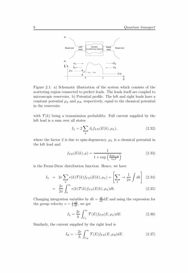
Landauer approach belongs to the viewpoint 2, i.e. a constant currentis forced to flow through a scattering system and the asking question iswhat the resulting potential distribution will be due to the spatially inho-mogeneous distribution of scatters [15]. Calculation of the current in theLandauer approach requires to divide formally the system into three parts,namely, the perfect leads and the scattering region, as depicted on Fig.(2.1).The leads, in turn, are connected to the infinite reservoirs which representthe infinity and contain many electrons in a local equilibrium character-ized by the Fermi-Dirac distribution function. The basic idea behind thisapproach is that the electron has a certain probability to transmit throughthe scattering region [16]. Hence, the current carrying by an electron in astate with a wave-vector k is
Jk = ev(k)T (k) (2.31)
8 Quantum transport
Sample
(scattering region)Left
leadRight
leadReservoir Reservoir
a)
b)
0 L
Figure 2.1: a) Schematic illustration of the system which consists of thescattering region connected to perfect leads. The leads itself are coupled tomicroscopic reservoirs. b) Potential profile. The left and right leads have aconstant potential µL and µR, respectively, equal to the chemical potentialin the reservoirs.
with T (k) being a transmission probability. Full current supplied by theleft lead is a sum over all states
IL = 2∑
k
JkfFD(E(k), µL), (2.32)
where the factor 2 is due to spin-degeneracy, µL is a chemical potential inthe left lead and
fFD(E(k), µ) =1
1 + exp(
E(k)−µkBT
) (2.33)
is the Fermi-Dirac distribution function. Hence, we have
IL = 2e∑
k
v(k)T (k)fFD(E(k), µL) =
[∑
k
→ 1
2π
∫
dk
]
(2.34)
=2e
2π
∫ ∞
0
v(k)T (k)fFD(E(k), µL)dk. (2.35)
Changing integration variables by dk = dkdEdE and using the expression for
the group velocity v = 1~
dEdk
, we get
IL =2e
h
∫ ∞
UL
T (E)fFD(E, µL)dE. (2.36)
Similarly, the current supplied by the right lead is
IR = −2e
h
∫ ∞
UR
T (E)fFD(E, µR)dE. (2.37)

S-matrix technique 9
Sum of both contributions gives the net current
I = IL + IR =2e
h
∫ ∞
UL
T (E) [fFD(E, µL) − fFD(E, µR)] dE. (2.38)
The potential drop between the reservoirs is
eV = µL − µR. (2.39)
In the case of very low bias, the Fermi-Dirac functions can be expanded inthe Taylor series
fFD(E, µL) − fFD(E, µR) ≈ −eV ∂fFD(E, µ)
∂E, (2.40)
which results in
I =2e
h
∫ ∞
UL
T (E)
[
−eV ∂fFD(E, µ)
∂E
]
dE. (2.41)
This equation allows to calculate conductance of the system
G =I
V=
2e2
h
∫ ∞
UL
T (E)
[
−∂fFD(E, µ)
∂E
]
dE. (2.42)
At a very low temperature the derivative of the Fermi-Dirac distributionfunction can be replaced by the Dirac delta function δ(E−µ) which reducesEq.(2.42) to
G =2e2
hT (µ). (2.43)
This equation shows that the conductance of the perfect conductor (i.e.T = 1) is finite and thus the resistance (G−1) is non-zero. The followingexplanation can be used [16]: in the contacts (reservoirs) the current iscarried by infinitely many transverse modes, however inside the conductoronly few modes supply the current. It leads to redistribution of the currentamong current-carrying modes which results in the interface resistance.
2.4 S-matrix technique
As it was shown in the previous section, the current (or conductance) can beformulated in terms of the transmission function T . The powerful methodto calculate T is the scattering matrix technique. Scattering matrix (or S-matrix) relates the outgoing amplitudes b = (b1, b2, ..., bn) to the incidentamplitudes a = (a1, a2, ..., an), see Fig.(2.1),
b = S(E)a, S(E) =
(r(E) t
′
(E)t(E) r
′
(E)
)
. (2.44)

10 Quantum transport
S matrix has a 2N · 2N dimension, where N is a number of transmissionchannels. The transmission probability now equals to
tm←n(E) = |Smn|2 (2.45)
Prior to calculation of the S-matrix, one can determine its general prop-erties. S-matrix must be unitary, that is a consequence of current conser-vation: the incoming electron flux
∑
n |a|2 must be equal to the outgoingflux
∑
n |b|2
b+b = a+a,
a+(1 − S+S)a = 0, (2.46)
S+S = I.
Moreover S-matrix is also a symmetric matrix, S = ST . This fact reflectsthe time-reversal symmetry of the Schrodinger equation, H = H∗. A non-zero magnetic field breaks the time-reversal symmetry. In this case, wehave S ~B = ST
− ~B.
S-matrix and Green’s function S-matrix can be expressed in terms ofGreen’s function. Outside the scattering region solution of the Schrodingerequation has the form of plane waves ψn(~r) ≈ eiknz, where we assume thatthe system with a cross-section area A is uniform in x and y directions, ~r =(~ρ, z). Each plane wave corresponds to a scattering channel n characterizedby a transverse momenta ~qn and longitudinal momenta kn with the energyE = (1/2m)(k2n + q2n). If we define the Green’s function G(E) = (E + iη −H)−1 with matrix elements between scattering channels m and n as
Gmn(z, z′, E) = A−1∫
d~ρ
∫
d~ρ′ exp (−i~qm~ρ) exp (−i~qn~ρ′)〈~r|G(E)|~r′〉.(2.47)
Then, the transmission coefficient, following Fisher and Lee [17], can becalculated as
tmn = −i~√vmvnGmn(z, z′, E) exp [−i(kmz − knz′)], (2.48)
where z and z′ are taken outside the scattering region, i.e. z > L andz′ < 0, see Fig.(2.1), and vn = kn/m is the velocity in channel n. Thisrelation is very important, since it shows the connection between differenttransport formalisms.

Chapter 3
Electron-electron interactions
With advent of quantum mechanics, the physical laws which govern par-ticles motion and interactions between particles became known. Howeverthe exact analytical solution is possible only for a system consisting of twoparticles. A typical piece of solid consists of approximately 1023 particles.Even if it would be possible to write down all the differential equationsrequired to describe this system, the solution of these equation is an un-feasible task in principle. The problem of finding the solution arises fromelectron-electron interaction which makes the motion of particles correlatedand couples corresponding differential equations. Therefore it is of greatimportance to develop approximated methods which provide a simplifiedform of the electron-electron interaction and reduces the number of equa-tions needed to be solved.
3.1 The many body problem
The Hamiltonian of a many-body system of interacting particle is writtenas
H = Te + Tn + Ve−e + Ve−n + Vn−n
= −∑
i
~2
2me
∇2i −
∑
I
~2
2MI
∇2I +
1
4πεε0
∑
i>j
e2
|~ri − ~rj |(3.1)
+1
4πεε0
∑
I>J
ZIZJe2
|~RI − ~RJ |− 1
4πεε0
∑
i,I
ZIe2
|~ri − ~RI |,
where the first two terms describe the kinetic energy of electrons and nuclei.The last three terms result from the Coulomb interaction between electrons,electron-nuclei and nuclei-nuclei respectively. The Hamiltonian acts on thewave-function Ψ({~ri}, {~RI}) which depends on the position of all electronsand nuclei in the system
HΨ({~ri}, {~RI}) = EΨ({~ri}, {~RI}). (3.2)
12 Electron-electron interactions
An essential simplification of Eq.(3.2) can be done with the use of the Born-Oppenheimer approximation which neglects the coupling between the nu-clei and electronic motion. In thermodynamic equilibrium electrons movemuch faster than nuclei, since M ≫ me, which allows to treat nuclei asstationary particles and neglect the kinetic term Tn in the Hamiltonian.Hence one can deal only with the electronic part, He, of the full Hamil-tonian which corresponds to the system of interacting electrons moving inthe effective potential produced by nuclei
He = Te + Ve−e + Ve−n + Vn−n, (3.3)
HeΦ({~ri}) = EΦ({~ri}). (3.4)
Even though electronic wave-function Φ({~ri}) still depends on the positions
of nuclei, ~RI are just parameters of Eq.(3.3) and the number of differentialequations needed to be solved is greatly reduced.
3.2 Hartree-Fock approximation
The Born-Oppenheimer approximation significantly simplifies the problemof interacting particles by eliminating the coupling between electrons andnuclear motion. However determination of the exact solution of the many-particle electronic wave-function is still not feasible. The basic idea ofthe Hartree-Fock approximation is to substitute the system of interactingelectrons by the motion of single electrons in the average self-consistentfield generated by all the other electrons in the system.
The Hamiltonian of the many-particle system is given by
H =∑
k
p2
2me+∑
k
V (~rk)+e2
8πεε0
∑
kk′
1
|~rk − ~rk′|=∑
k
Hk+∑
kk′
Hkk′, (3.5)
where the term V (~rk) =∑
I V (~rk − ~RI) describes interaction between k-
electron with all nuclei in the system located at {~RI}. The operator Hk is aone-particle operator, while Hkk′ depends on the position of two particles.
The simplest way to construct the many-particle wave-function is towrite down it in the form of a product of single-particle wave-functions,φk(~r), which have to be determined,
Φ({~rk}) =∏
k
φ(~rk), 〈φi(~r)|φj(~r)〉 = δij . (3.6)
Let us calculate an expectation value of the energy [14]
E = 〈Φ|H|Φ〉 =∑
k
〈φk|Hk|φk〉 +e2
8πεε0
∑
kk′
⟨
φkφk′
∣∣∣∣
1
~rk − ~rk′
∣∣∣∣φkφk′
⟩
.
(3.7)

Hartree-Fock approximation 13
According to the variational principle the closer values of φk to the exactsolution the smaller value of the energy, thus
δ
(
E −∑
k
Ek (〈φk|φk〉 − 1)
)
= 0, (3.8)
where Ek are Lagrange parameters. Changing φi → φi + δφi and keepingterms linear in respect to δφi, we arrive at the Hartree equation[
− ~2
2me
∆ + V (~r) +e2
4πεε0
∑
k 6=i
∫ |φk(~rk)|2|~rk − ~ri|
d~rk
]
φi(~r) = Eiφi(~r). (3.9)
The third term in the brackets has a simple interpretation. If we define thecharge density as n(~r) = e
∑
i |φi(~r)|2, then the term
UH(~r) =e
4πεε0
∫n(~r′)
|~r′ − ~r|d~r′, (3.10)
called the Hartree term, describes the Coulomb interaction between thei-th electron located at ~r with all the other electrons in the system.
Since electrons are fermions, the many-particle wave-function must changethe sign under the interchange of the coordinates of any two particles. Thewave-function given by Eq.(3.6) does not satisfy this condition. In order toconstruct an antisymmetric wave-function one can use Slater determinant
Φ({~qk}) =1√N !
∣∣∣∣∣∣∣
φ1(~q1) . . . φN(~q1)...
. . ....
φ1(~qN) . . . φN(~qN)
∣∣∣∣∣∣∣
, (3.11)
where ~qi = {~ri, σi} denotes both position and spin of the electron and thefactor 1√
N !is used for normalization. Following the same way as before, i.e.
applying the variational principle to the expectation value of the energy,the new form of the wave-function results in the equation [14]
(
− ~2
2me∆ + V (~r)
)
φi(~r) +e2
4πεε0
∑
k 6=i
∫ |φk(~r′)|2|~r′ − ~r|
d~r′φi(~r)
− e2
4πεε0
∑
k 6=i
∫φ∗k(~r
′)φi(~r′)
|~r′ − ~r|d~r′ · φk(~r) = Eiφi(~r), (3.12)
called the Hartree-Fock equation. The additional term in Eq.(3.12) isknown as the exchange interaction. It does not have classical analog andresults from the Pauli exclusion principle. The exchange interaction termwhich arises in the Hartree-Fock approximation has a non-local form incontrast to the Coulomb interaction. This makes calculations more com-plicated. In the density-functional theory (discussed in Sec.(3.3)) a numberof approximations are used to deduce a local form of the exchange interac-tion.

14 Electron-electron interactions
3.3 Density-functional theory
Density-functional theory (DFT) is one of the most widely used model-ing method applied in physics and chemistry for calculation of electronicproperties of complex systems. The basic idea behind DFT is to describethe system in terms of the electronic density instead of operating with amany-body wave function [18].
Hohenberg-Kohn theorems
In 1964 Hohenberg and Kohn proved two theorems which made the DFTpossible [19]. They state that a knowledge of the ground-state densitycan, in principle, determine all the ground-state properties of a many-bodysystem [18].
Theorem 1: An external potential Vext(~r) uniquely determines the elec-tronic density for any system of interacting particles.
Proof: Assume that the same electron density n(~r) results from two po-tentials V 1
ext(~r) and V 2ext(~r) differing by more than constant. Obviously,
V 1ext(~r) and V 2
ext(~r) belong to distinct Hamiltonians H1(~r) and H2(~r) whichproduce different wave-functions Ψ1(~r) and Ψ2(~r). The ground-state stateenergy associated with the Hamiltonian H1(~r) is
E1 = 〈Ψ1|H1|Ψ1〉. (3.13)
According to the variational principle no other wave-function can give lowerenergy, i.e.
E1 = 〈Ψ1|H1|Ψ1〉 < 〈Ψ2|H1|Ψ2〉 (3.14)
Since the Hamiltonians differs by the external potentials only, we can writeH1 = H2 + V 1
ext − V 2ext, which gives us for the expectation value
〈Ψ2|H1|Ψ2〉 = 〈Ψ2|H2|Ψ2〉 +
∫[V 1ext − V 2
ext
]n(~r)d~r. (3.15)
Substituting it into Eq.(3.14) and recalling that E2 = 〈Ψ2|H2|Ψ2〉, weobtain
E1 < E2 +
∫[V 1ext − V 2
ext
]n(~r)d~r. (3.16)
Interchanging labels (1) and (2), we find in the same way that
E2 < E1 +
∫[V 2ext − V 1
ext
]n(~r)d~r. (3.17)
Addition of Eq.(3.16) and Eq.(3.17) leads to contradiction
E1 + E2 < E1 + E2. (3.18)
Hence the theorem is proved by reductio ad absurdum.
Kohn-Sham equations 15
Theorem 2: The exact ground-state density n(~r) is the global minimumof the universal functional F [n].
Proof: Since the electron density n(~r) uniquely determines wave-functionΨ, the universal functional F [n] can be defined as
F [n] = 〈Ψ|T + Ue−e|Ψ〉. (3.19)
For a given external potential Vext(~r), the energy functional is written as
E[n] = F [n] +
∫
Vext(~r)n(~r)d~r. (3.20)
According to the variational principle, it has a minimum only for theground-state wave-function Ψ. For any other wave-function Ψ′ which pro-duces density n′(~r), we get
E[Ψ] = F [n]+
∫
Vext(~r)n(~r)d~r < F [n′]+
∫
Vext(~r)n′(~r)d~r = E[Ψ′]. (3.21)
3.4 Kohn-Sham equations
In the Kohn-Sham method [20] one considers a system of non-interactingelectrons moving in some effective potential veff(~r) (which will be definedlater)
(
− ~2
2m∇2 + veff (~r)
)
φi(~r) = ǫiφi(~r). (3.22)
An obtained set of the Kohn-Sham orbitals φi determines the electrondensity
n(~r) =∑
i
|φi(~r)|2. (3.23)
The energy functional equals to
E[n] = TS[n] + Veff [n] = TS[n] +
∫
n(~r)vext(~r)d~r+ VH [n] +Exc[n], (3.24)
where the first term,
Ts[n] =
N∑
i=1
∫
φ∗i (~r)
(
− ~2
2m∇2
)
φi(~r)d~r, (3.25)
is a single-electron kinetic energy functional. The second term describes thepotential energy acquired by the charged particles in an external electricfield. The Hartree term is given by
VH =e2
8πεε0
∫ ∫n(~r)n(~r′)
|~r − ~r′|d~rd~r′. (3.26)
16 Electron-electron interactions
The last term, Exc[n], arises from the exchange-correlation interaction. Itcan be shown [21] that the functional given by Eq.(3.24) corresponds tothe the effective potential in the form
veff(~r) = vext(~r) +e
4πεε0
∫n(~r′)
|~r − ~r′|d~r′ + vxc(~r). (3.27)
Equations (3.22), (3.23) and (3.27) constitute the basis of the Kohn-Shammethod, and are solved self-consistently for the ground state density andthe effective potential.
The explicit form of the exchange-correlation potential vxc can be de-termined using other approximations. The most widely used are the localspin density approximation [21] and the generalized gradient approximation[22].
3.5 Thomas-Fermi-Dirac approximation
According to the Hohenberg-Kohn theorems discussed in Sec.(3.3), thetotal energy of the system may be written as
E[n(~r)] =
∫
T [n(~r)]d~r +
∫
V (~r)n(~r)d~r, (3.28)
where T [n(~r)] is a kinetic energy functional of the electron density n(~r) andV (~r) is an external potential. The Thomas-Fermi approximation assumesthat the kinetic-energy functional is a local function of the density. Thisassumption allows to rewrite Eq.(3.28) in the form
µ = T [n(~r)] + V (~r). (3.29)
Let us now derive the relation between the potential and charge densityin graphene. Taking into account dispersion relation for graphene, E =
±~vF |~k|, and using n = gvgs∫
d~k(2π)2
(vF = 106 m/s and gv = gs = 2, see
Chapter 4 for details), we get [28]
sgn[n(~r)]~vF√
πn(~r) + V (~r) = µ. (3.30)
An alternative way is to rewrite Eq.(3.28) in the form which directly relateselectron density to the external potential [23, 24]
n(~r) =
∫
dEρ(E − V (~r))fFD(E, µ), (3.31)
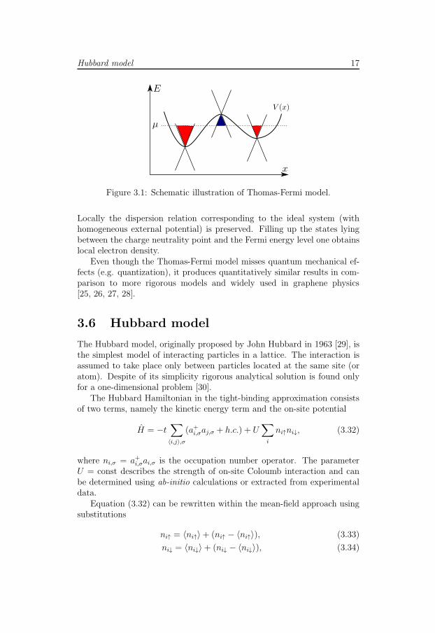
where ρ(E) is a single-electron density of states, calculated in the presenceof homogeneous potential. Figure (3.1) illustrates application of Eq.(3.31).
Hubbard model 17
Figure 3.1: Schematic illustration of Thomas-Fermi model.
Locally the dispersion relation corresponding to the ideal system (withhomogeneous external potential) is preserved. Filling up the states lyingbetween the charge neutrality point and the Fermi energy level one obtainslocal electron density.
Even though the Thomas-Fermi model misses quantum mechanical ef-fects (e.g. quantization), it produces quantitatively similar results in com-parison to more rigorous models and widely used in graphene physics[25, 26, 27, 28].
3.6 Hubbard model
The Hubbard model, originally proposed by John Hubbard in 1963 [29], isthe simplest model of interacting particles in a lattice. The interaction isassumed to take place only between particles located at the same site (oratom). Despite of its simplicity rigorous analytical solution is found onlyfor a one-dimensional problem [30].
The Hubbard Hamiltonian in the tight-binding approximation consistsof two terms, namely the kinetic energy term and the on-site potential
H = −t∑
〈i,j〉,σ(a+i,σaj,σ + h.c.) + U
∑
i
ni↑ni↓, (3.32)
where ni,σ = a+i,σai,σ is the occupation number operator. The parameterU = const describes the strength of on-site Coloumb interaction and canbe determined using ab-initio calculations or extracted from experimentaldata.
Equation (3.32) can be rewritten within the mean-field approach usingsubstitutions
ni↑ = 〈ni↑〉 + (ni↑ − 〈ni↑〉), (3.33)
ni↓ = 〈ni↓〉 + (ni↓ − 〈ni↓〉), (3.34)
18 Electron-electron interactions
where 〈niσ〉 denotes average occupation of spin σ at site i. Hence, we have
ni↑ni↓ = ni↑〈ni↓〉+ni↓〈ni↑〉− 〈ni↓〉〈ni↑〉+ (ni↑ − 〈ni↑〉)(ni↓ − 〈ni↓〉)︸ ︷︷ ︸
≈0
, (3.35)
where the product of two deviations from the average values is assumedto be small. Substituting the result of Eq.(3.35) into Eq.(3.32) we deriveHubbard Hamiltonian in the mean-field approximation
HMF = −t∑
〈i,j〉,σ(a+i,σaj,σ + h.c.) + U
∑
i
(ni↑〈ni↓〉 + ni↓〈ni↑〉 − 〈ni↓〉〈ni↑〉) .
(3.36)Despite of its simplicity the Hubbard model was applied to investigate theproperties of different materials. It reproduces a variety of phenomenaobserved in solid state physics, such as ferromagnetism, metal-insulatortransition and superconductivity.

Chapter 4
Electronic structure and
transport in graphene
4.1 Basic electronic properties
y
x
A
Ba) b)
Figure 4.1: a) Graphene lattice consisting of two interpenetrating triangu-lar sublattices A (red circles) and B (blue circles) with unit vectors ~a1, ~a2and nearest-neighbours vectors ~δ1, ~δ2, ~δ3. The yellow parallelogram marksunit cell containing two atoms. b) The structure of reciprocal lattice de-
fined by unit vectors ~b1 and ~b2. The grey hexagon is the first Brillouinzone.
Real space and reciprocal lattices Carbon atoms in graphene arearranged in a honeycomb lattice shown on Fig.(4.1). This structure can bedescribed [31, 32] as a triangular lattice with unit vectors
~a1 =acc2
(3,√
3),~a2 =acc2
(3,−√
3), (4.1)

20 Electronic structure and transport in graphene
where acc = 0.142 nm is a carbon-carbon distance. Unit cell contains twoatoms and has an area Scell = a
√3
4, where a = acc
√3 = 0.246 nm is a
lattice constant. Each point of the sublattice A is connected to its nearest-neighbors by the vectors
~δ1 = acc
(
1
2,
√3
2
)
, ~δ2 = acc
(
1
2,−
√3
2
)
, ~δ3 = acc (−1, 0) . (4.2)
For a given lattice one can easily build a reciprocal lattice with a unitvectors ~bi defined by the relation ~bi~aj = 2πδij , i.e.
~b1 =2π
3acc(1,
√3),~b2 =
2π
3acc(1,−
√3). (4.3)
The first Brillouin zone, which is the Wigner-Seitz primitive cell of thereciprocal lattice [33], is shown on Fig.(4.1)(b). There are two inequivalentpoints which are of special interest in graphene physics
~K =2π
3acc
(
1,1√3
)
, ~K ′ =2π
3acc
(
1,− 1√3
)
. (4.4)
Dispersion relation Graphene lattice can be considered as two inter-penetrating triangular sublattices A and B which are defined by vectors
~RAp,q = p~a1 + q~a2, ~R
Bp,q = ~δ1 + p~a1 + q~a2, (4.5)
where p, q are integer numbers.In a single-electron approximation the tight-binding Hamiltonian for
electrons in graphene is given by
Htb = −t∑
p,q
(a+p,qbp,q + a+p,qbp−1,q + a+p,qbp−1,q+1
)+ h.c., (4.6)
where a+p,q(ap,q) and b+p,q(bp,q) create (annihilate) an electron on sublattices
A and B at site ~RAp,q and ~RB
p,q respectively and t = 2.77 eV is a nearest-neighbor hopping integral.
The wave-function for the lattice can be written in the form
|Ψ〉 =∑
p,q
(ζAp,qa
+p,q + ζBp,qb
+p,q
)|0〉, (4.7)
where ζA(B)p,q is a probability amplitude to find the electron at site
~R
A(B)p,q
Substituting Eqs.(4.6),(4.7) into the Schrodinger equation, Htb|Ψ〉 = E|Ψ〉,and calculating the matrix elements 〈0|ap,qHtba
+p,q|0〉 and 〈0|bp,qHtbb
+p,q|0〉

Basic electronic properties 21
with use of the commutation relation, one arrives to the system of differenceequations
−t(ζBp,q + ζBp−1,q + ζBp−1,q+1
)= EζAp,q, (4.8)
−t(ζAp,q + ζAp+1,q + ζAp+1,q+1
)= EζBp,q.
The states ζAp,q and ζBp,q can be written in the Bloch form
ζAp,q = ψAp,qe
i~k ~RAp,q , ψA
p,q = ψAp+1,q = ψA
p+1,q−1, (4.9)
ζBp,q = ψBp,qe
i~k ~RBp,q , ψB
p,q = ψBp−1,q = ψB
p−1,q+1.
Substituting Eq.(4.9) and Eq.(4.2) into Eq.(4.8) and omitting indexes(p, q), one gets
−tφ(~k)ψB = EψA, (4.10)
−tφ∗(~k)ψA = EψB,
whereφ(~k) ≡ ei
~k ~δ1 + ei~k ~δ2 + ei
~k ~δ3 , (4.11)
or in a matrix form
H
(ψA
ψB
)
= E
(ψA
ψB
)
, H ≡(
0 −tφ(~k)
−tφ∗(~k) 0
)
. (4.12)
In order to obtain dispersion relation, one needs to determine the eigenval-ues of the matrix H, which are calculated using the relation det |H− IE| =0,
E(~k)2 = t2|φ(~k)|2,
E(~k) = ±t
√√√√1 + 4 cos2
(√3
2accky
)
+ 4 cos
(√3
2accky
)
cos
(3
2acckx
)
.
(4.13)
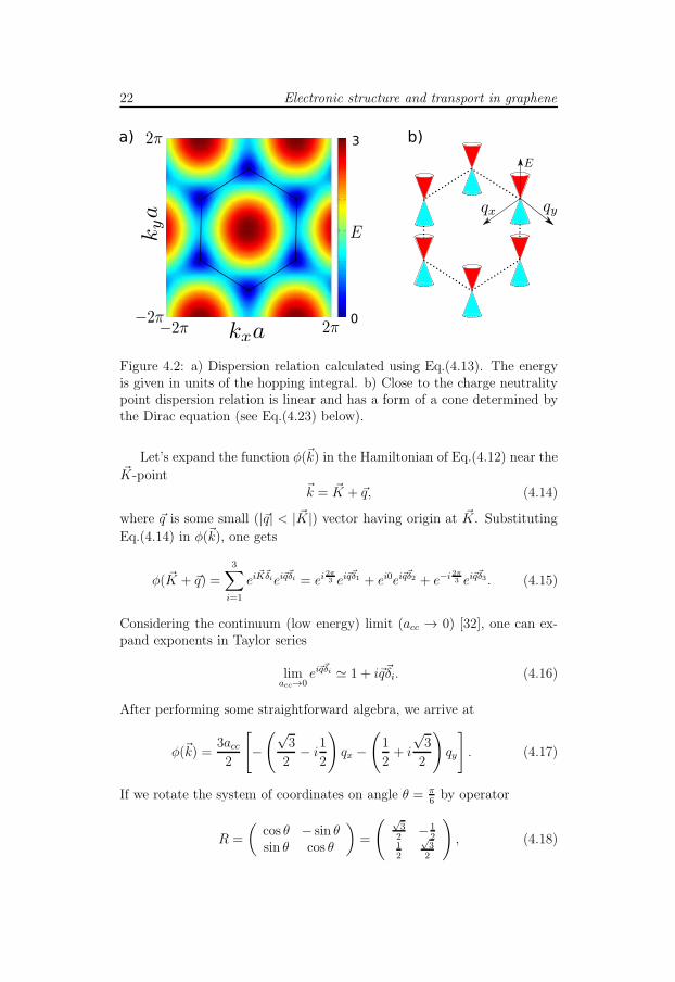
Dirac equation The spectrum of graphene, given by Eq.(4.13), is sym-metric in respect to energy E = 0. If the Fermi energy coincides withthis point (EF = 0), i.e the states are occupied only up to zero energy,it corresponds to the case of electrically neutral graphene. One is usuallyinterested in electronic properties close to a charge-neutrality point. Thereare six points in the k-space where the energy equals to zero. These pointsare at the corners of the first Brillouin zone, see Fig.(4.1). Only two of
them, ~K and ~K ′, are inequivalent.
22 Electronic structure and transport in graphene
0
3a) b)
Figure 4.2: a) Dispersion relation calculated using Eq.(4.13). The energyis given in units of the hopping integral. b) Close to the charge neutralitypoint dispersion relation is linear and has a form of a cone determined bythe Dirac equation (see Eq.(4.23) below).
Let’s expand the function φ(~k) in the Hamiltonian of Eq.(4.12) near the~K-point
~k = ~K + ~q, (4.14)
where ~q is some small (|~q| < | ~K|) vector having origin at ~K. Substituting
Eq.(4.14) in φ(~k), one gets
φ( ~K + ~q) =
3∑
i=1
ei~K~δiei~q
~δi = ei2π3 ei~q
~δ1 + ei0ei~q~δ2 + e−i
2π3 ei~q
~δ3 . (4.15)
Considering the continuum (low energy) limit (acc → 0) [32], one can ex-pand exponents in Taylor series
limacc→0
ei~q~δi ≃ 1 + i~q~δi. (4.16)
After performing some straightforward algebra, we arrive at
φ(~k) =3acc
2
[
−(√
3
2− i
1
2
)
qx −(
1
2+ i
√3
2
)
qy
]
. (4.17)
If we rotate the system of coordinates on angle θ = π6
by operator
R =
(cos θ − sin θsin θ cos θ
)
=
( √32
−12
12
√32
)
, (4.18)

Basic electronic properties 23
Eq.(4.15) is finally reduced to
φ(~q) = −3acc2
(qx + iqy). (4.19)
Substituting Eq.(4.19) into Eq.(4.12), one gets
3
2acct
(0 qx + iqy
qx − iqy 0
)(ψA
ψB
)
= E
(ψA
ψB
)
. (4.20)
With the use of the Pauli matrices, ~σ = (σx, σy), where
σx =
(0 11 0
)
, σy =
(0 −ii 0
)
, (4.21)
the Hamiltonian can be written in a vector form
HK = ~vF~σ~q, (4.22)
where vF = 32acct~
≃ 106 m/s is a Fermi velocity. Equation (4.22) is al-gebraically identical to a two-dimensional relativistic Dirac equation withvanishing rest mass known as Weyl’s equation for a neutrino, where thetwo-component wave function (or spinor) represents pseudo-spin which re-sults from the presence of two sublattices [34, 35]. The eigenenergies of HK
are
E = ±~vF q. (4.23)
In order to find eigenfunctions Eq.(4.20) can be rewritten in the followingway
~vF q
(0 eiθ(~q)
e−iθ(~q) 0
)(ψA
ψB
)
= E
(ψA
ψB
)
, (4.24)
where θ(~q) = arctan(qy/qx). Taking into account Eq.(4.23) for eigenener-gies and using normalization condition |ψA|2 + |ψB|2 = 1, one gets
|Ψ ~K,s(~q)〉 =1√2
(eiθ(~q)/2
se−iθ(~q)/2
)
, (4.25)
where the sign s = ± corresponds to the eigenenergies ±~vF q.Besides spin-degeneracy each level is double-degenerated due to valley.
One has to operate by a full wave function which includes the contributionfrom both valleys. The same procedure can be repeated to obtain theeffective Hamiltonian and wave function near K ′-point
HK ′ = ~vF~σ∗~q, |Ψ ~K ′,s(~q)〉 =
1√2
(e−iθ(~q)/2
seiθ(~q)/2
)
. (4.26)
24 Electronic structure and transport in graphene
If the wave-vector ~q rotates once around the Dirac point, i.e. θ →θ + 2π, the wave-function acquires an additional phase equals to π, henceΨ ~K,s(θ ± 2π) = −Ψ ~K,s(θ) which is a characteristics of fermions.
Electron’s wave function in graphene has a chiral nature. Helicity canbe interpreted as a projection of pseudospin vector on direction of motionand defined by the operator h = ~σ~q/|~q|. It can be easily shown usingEq.(4.22), that eigenvalues of the helicity operator equal to h = ±1. Sinceh commutes with the Hamiltonian, helicity is a conserved quantity andresponsible for such effects as the Klein tunneling [36].
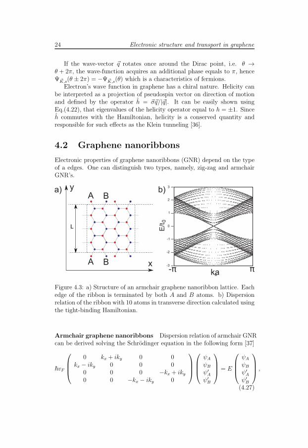
4.2 Graphene nanoribbons
Electronic properties of graphene nanoribbons (GNR) depend on the typeof a edges. One can distinguish two types, namely, zig-zag and armchairGNR’s.
-3
-2
-1
0
1
2
3
E/t0
π-π kax
a) b)
L
Figure 4.3: a) Structure of an armchair graphene nanoribbon lattice. Eachedge of the ribbon is terminated by both A and B atoms. b) Dispersionrelation of the ribbon with 10 atoms in transverse direction calculated usingthe tight-binding Hamiltonian.
Armchair graphene nanoribbons Dispersion relation of armchair GNRcan be derived solving the Schrodinger equation in the following form [37]
~vF
0 kx + iky 0 0kx − iky 0 0 0
0 0 0 −kx + iky0 0 −kx − iky 0
ψA
ψB
ψ′Aψ′B
= E
ψA
ψB
ψ′Aψ′B
,
(4.27)

Graphene nanoribbons 25
where ψA(B) and ψ′A(B) are the probabilty amplitudes on the sublattice
A(B) for the state near the ~K and ~K ′ points, respectively. The total wavefunction has the form
Ψ = ei~K~rΨ ~K + ei
~K ′~rΨ′~K . (4.28)
Let us first find a solution near the K point. Substituting in Eq.(4.22)
wave vector ~k =(
−i ∂∂x,−i ∂
∂y
)
, one gets
(0 −i ∂
∂x+ ∂
∂y
−i ∂∂x
− ∂∂y
0
)(ψA
ψB
)
= ǫ
(ψA
ψB
)
, (4.29)
where ǫ = E~vF
. Due to translational invariance in ~x-direction the wavefunction can be written in the form
Ψ ~K(x, y) = eikxx(φA(y)φB(y)
)
, (4.30)
which allows us to reduce the problem to a system of two differential equa-tions{
kxφB(y) + ∂φB(y)∂y
= ǫφA(y)
kxφA(y) − ∂φA(y)∂y
= ǫφB(y)⇒{
φB(y) = kxǫφA(y) − 1
ǫ∂φA(y)
∂y∂2φA(y)
∂y2+ z2φA(y) = 0
(4.31)where z2 = ǫ2 − k2x. The general solution of the system of equations is asum of plane waves
{φA(y) = Aeizy +Be−izy
φB(y) = kx−izǫAeizy + kx+iz
ǫBe−izy
(4.32)
Similar derivation can be done for the wave functions describing the statesnear K ′-point, which gives
{φ′A(y) = Ceizy +De−izy
φ′B(y) = −kx−izǫ
Ceizy + −kx+izǫ
De−izy(4.33)
In order to find the unknown coefficients A and B, one can utilize theboundary conditions. The armchair nanoribbon edge consist of atoms be-longing to both sublattices, see Fig.(4.3)(a), therefore one can expect thatboth ΨA and ΨB should vanish at the edges
ΨA(0) = ΨB(0) = ΨA(L) = ΨB(L) = 0, (4.34)
where ΨA(B) is an A(B) component of the total wave function (4.28).Hence, we have
φA(0) + φ′A(0) = 0φB(0) + φ′B(0) = 0
eiKyLφA(L) + e−iKyLφ′A(L) = 0eiKyLφB(L) + e−iKyLφ′B(L) = 0
(4.35)

26 Electronic structure and transport in graphene
Substituting Eq.(4.32) and Eq.(4.33) into Eq.(4.35) and solving the systemof four unknowns, we arrive at
e2izL = ei∆KyL, (4.36)
where ∆Ky = 4π3a
. Therefore, the allowed values of z are
z =πn
L+
2π
3a. (4.37)
Finally, the dispersion relation is given by
E = ±~vF
√
k2x +
(πn
L+
2π
3a
)2
. (4.38)
Note that if the ribbon consists of 3N + 1 atoms, Eq.(4.38) allows zeroenergy solutions when kx → 0. This kind of ribbons are called metallic.Otherwise the dispersion relation posses an energy gap, i.e. the ribbons aresemiconducting.
-3
-2
-1
0
1
2
3
E/t0
π-π kax
a) b)
L
Figure 4.4: a) Structure of a zig-zag graphene nanoribbon lattice. Eachedge of the ribbon is terminated by either A or B atoms. b) Dispersionrelation of the ribbon with 10 atoms in transverse direction calculated usingthe tight-binding Hamiltonian.
Zig-zag graphene nanoribbons The Hamiltonian describing zig-zagGNR can be derived from the Hamiltonian used for armchair GNR byrotation of the system on angle π
2, i.e. changing kx → ky and ky → −kx
(0 i ∂
∂y+ ∂
∂x
i ∂∂y
− ∂∂x
0
)(ψA
ψB
)
= ǫ
(ψA
ψB
)
. (4.39)

Warping 27
Substituting the wave function in the form given by Eq.(4.30) and followingthe same procedure as in the case of the armchair GNR, we get
{φA(y) = Aeizy +Be−izy
φB(y) = −ikx−zǫ
Aeizy + −ikx+zǫ
Be−izy(4.40)
For zig-zag nanoribbons, as illustrated in Fig.(4.4), the boundary conditionsare
φA(L) = φB(0) = 0. (4.41)
Solving the system of linear equation, we derive the relation between kxand z
e−i2zL =ikx + z
ikx − z(4.42)
In contrast to armchair nanoribbons, the transverse and longitudinal com-ponents of the wave vector are coupled in zGNR. Another interesting fea-ture of zGNR is an existence of surface states. Besides the solutions withreal z describing propagating states the transcendental equation (4.42) sup-ports also solutions with imaginary values of z. It corresponds to the so-called edge (or surface) states, i.e the states spatially localized near theedges.
4.3 Warping
c
Figure 4.5: a)Experimental 3D constant current STM image of singlelayer graphene adopted from Ref.[40] b) Generated surface of a corrugatedgraphene sheet [39]. Black line corresponds to a characteristic wave-lengthof the ripples. c) Magnified area marked in a) by black rectangular. M andS stands for maximum (minimum) and saddle points, respectively.
Graphene is a pure two-dimensional crystal. According to the Mermin-Wagner theorem, the long-range order of 2D crystals should be destroyed
28 Electronic structure and transport in graphene
by long-wavelength fluctuations and therefore 2D membranes have a ten-dency to get crumpled being in a 3D space [38]. In the case of grapheneminimization of energy results in appearance of ripples on graphene sheet.The existence of the ripples was confirmed by a number of experiments[40, 41]. Warping can effect electronic properties. For example, bendingthe graphene plane changes overlap between p orbitals and in turn hoppingintegrals in the tight-binding model. Also warping can be related to theformation of electron-hole puddels which cause the spatial modulation ofcharge density [42]. Another example is a magnetotransport. Electronspropagating through a warped graphene subjected to a magnetic field areinfluenced by spatially correlated effective magnetic field.
The corrugated surface of graphene can be modeled [see Fig.(4.5)] by asuperposition of plane waves
h(~r) = C∑
i
Cqi sin(~qi~ri + δi), (4.43)
where h(~r) is a out-of-plane displacement at point defined by in-plane posi-tion vector ~r = (x, y). The directions ϕi of wave vectors ~qi = |qi|(cosϕi, sinϕi)and the phases δi were chosen randomly. The length of the wave vectorsqi covers equidistantly the range 2π/L < qi < 2π/(3acc), where L is aleading linear size of the rectangular area and acc denotes the C-C bondlength (we assume that L ≫ λ∗). The amplitude of the mode was given
by the harmonic approximation Cq =√
2⟨h2q⟩
for the wave length λ < λ∗,
otherwise it was kept constant and equal to Cq∗ , where q∗ = 2π/λ∗. Weintroduced the normalization constant C to keep the averaged amplitudeof the out-of-plane displacement h =
√
2 〈h2〉 equal to the experimentalvalues h ≈ 1 nm for typical sizes of samples.
4.4 Bilayer graphene
In a tight-binding approximation bilayer grpahene can be modeled by thefollowing Hamiltonian [31]
H = − t∑
i;l=1,2
(a+l,ibl,i+∆ + h.c.)
− γ1∑
i
(a+1,ia2,i + h.c.)
− γ3∑
i
(b+1,ib2,i+∆ + h.c.), (4.44)
where a+l,i (al,i) and b+l,i (bl,i) are the creation (annihilation) operators for
sublattice A (B), in the layer l = 1, 2, at site ~Ri, where i = (p, q). The
Bilayer graphene 29
γ1γ3
γ4
tAB
AB
11
22
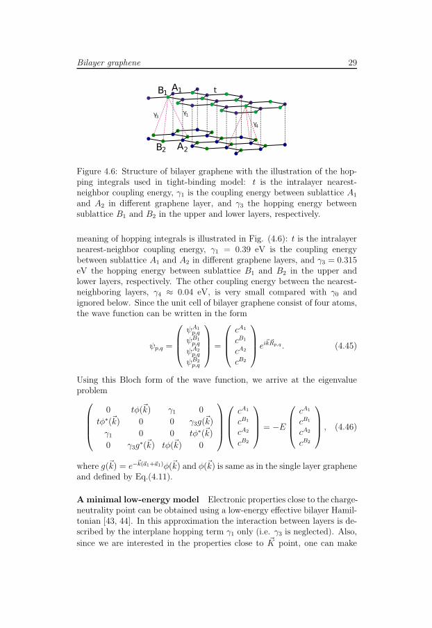
Figure 4.6: Structure of bilayer graphene with the illustration of the hop-ping integrals used in tight-binding model: t is the intralayer nearest-neighbor coupling energy, γ1 is the coupling energy between sublattice A1
and A2 in different graphene layer, and γ3 the hopping energy betweensublattice B1 and B2 in the upper and lower layers, respectively.
meaning of hopping integrals is illustrated in Fig. (4.6): t is the intralayernearest-neighbor coupling energy, γ1 = 0.39 eV is the coupling energybetween sublattice A1 and A2 in different graphene layers, and γ3 = 0.315eV the hopping energy between sublattice B1 and B2 in the upper andlower layers, respectively. The other coupling energy between the nearest-neighboring layers, γ4 ≈ 0.04 eV, is very small compared with γ0 andignored below. Since the unit cell of bilayer graphene consist of four atoms,the wave function can be written in the form
ψp,q =
ψA1p,q
ψB1p,q
ψA2p,q
ψB2p,q
=
cA1
cB1
cA2
cB2
ei~k ~Rp,q . (4.45)
Using this Bloch form of the wave function, we arrive at the eigenvalueproblem
0 tφ(~k) γ1 0
tφ∗(~k) 0 0 γ3g(~k)
γ1 0 0 tφ∗(~k)
0 γ3g∗(~k) tφ(~k) 0
cA1
cB1
cA2
cB2
= −E
cA1
cB1
cA2
cB2
, (4.46)
where g(~k) = e−~k(~a1+~a1)φ(~k) and φ(~k) is same as in the single layer graphene
and defined by Eq.(4.11).
A minimal low-energy model Electronic properties close to the charge-neutrality point can be obtained using a low-energy effective bilayer Hamil-tonian [43, 44]. In this approximation the interaction between layers is de-scribed by the interplane hopping term γ1 only (i.e. γ3 is neglected). Also,
since we are interested in the properties close to ~K point, one can make

30 Electronic structure and transport in graphene
the expansion −tφ(~k) ≈ ~vFk, where k = kx + iky. Taking into accountthese approximations, one gets
H =
0 ~vFk γ1 0~vFk
∗ 0 0 0γ1 0 0 ~vFk
∗
0 0 ~vFk 0
. (4.47)
Solution of det(H − EI) = 0 gives a dispersion relation
E(~k) = s1
(
s2γ12
+
√
γ214
+ ~2v2Fk2
)
, (4.48)
where s1, s2 = ±1. One can consider this equation in two limits (belowonly the conduction band is discussed):
a) low energies, ~vFk < γ1
E(~k) = s2γ12
+
√
γ214
+ ~2v2Fk2
︸ ︷︷ ︸
γ12
(
1+2~2v2
Fk2
γ21
)
≈ s2γ12
+γ12
+~2v2Fk
2
γ21, (4.49)
E(k) ≈{
~2v2F k2
γ1, s2 = −1
γ1 +~2v2F k2
γ1, s2 = 1
(4.50)
Equations (4.50) show that the conduction band of bilayer graphene con-sists of two parabolic bands separated by the energy interval γ1. In thevicinity of the Dirac point the dispersion relation of the lowest subbandcan be rewritten in a form which is usually used in a conventional 2DEGsystems, i.e.
E =~2k2
2m∗, (4.51)
where m∗ ≡ γ12v2F
is an effective mass.
b) high energies, ~vFk > γ1
E(~k) = s2γ12
+
√
γ214
+ ~2v2Fk2
︸ ︷︷ ︸
~vF k
(
1+γ21
8~2v2F
k2
)
≈ s2γ12
+ ~2v2Fk
2, (4.52)
E(k) ≈{
~vFk, s2 = −1~vFk + γ1, s2 = 1
(4.53)
i.e. the dispersion relation consists of two linear bands (as in the case ofthe the single layer graphene) separated by the energy interval γ1.

Dirac fermions in a magnetic field 31
Biased bilayer graphene Electronic properties of bilayer graphene canbe strongly modified by applying external electric field, which causes apotential difference between layers. In this case the Hamiltonian (4.47) ismodified
H =
U1 ~vFk γ1 0~vFk
∗ U1 0 0γ1 0 U2 ~vFk
∗
0 0 ~vFk U2
, (4.54)
where U1 and U2 are on-site energies or electrostatic potentials of the 1-st and 2-nd layer respectively. The dispersion relation of biased bilayergraphene is
E±,s(~k) = U1+U2
2
±√
∆U2
4+ ~2v2Fk
2 + γ2
2+ (−1)s
√
(∆U2 + γ2)~2v2Fk2 + γ4
4,
(4.55)
where ∆U = U2 − U1 and s = ±1.
Energy gap, ∆Eg, in the vicinity of ~K-point is determined by
∆Eg = E+,1(0) − E−,1(0) = U2 − U1 = ∆U. (4.56)
This equation shows that a band-gap can be tuned by application of anexternal voltage. This makes bilayer graphene a promising candidate forfuture electronics.
4.5 Dirac fermions in a magnetic field
In a high enough perpendicular magnetic field a continues spectrum of any2DEG systems is usually modified into a series of Landau levels (LLs).Since the behavior of electrons in graphene described by Dirac rather thanSchrodinger equation it should be reflected in the spectrum as well. Westart the calculation of the dispersion relation from the Hamiltonian givenby Eq.(4.22)
H = vF~σ~p. (4.57)
In a magnetic field the canonical momentum is changed to ~p → ~~k + e ~A,where ~A is a vector potential of the magnetic field. Using the Landau gaugein the form ~A = (−By, 0, 0), one gets
H = vF
[(
−i~ ∂
∂x− eBy
)(0 11 0
)
+
(
−i~ ∂∂y
)(0 −ii 0
)]
. (4.58)

32 Electronic structure and transport in graphene
Substituting it in the Schrodinger equation, H|Ψ〉 = E|Ψ〉, one arrives atthe eigenvalue problem
vF
(0 −i~ ∂
∂x− eBy − ~
∂∂y
−i~ ∂∂x
− eBy + ~∂∂y
0
)(ψA
ψB
)
= E
(ψA
ψB
)
.
(4.59)Due to translational invariance in ~x direction, the solution of the Schrodingerequation with the Hamiltonian (4.58) can be written in the Bloch form
|Ψ(x, y)〉 =
(ψA
ψB
)
= eikx(φA(y)φB(y)
)
, (4.60)
which gives
−~vF
(0 ∂
∂y+ y
lB− lBk
− ∂∂y
+ ylB
− lBk 0
)(φA(y)φB(y)
)
= lBE
(φA(y)φB(y)
)
,
(4.61)
where lB =√
~
eBis a magnetic length. Introducing dimensionless length
scale ζ = ylB
− lBk, one finally gets
(0 ∂
∂ζ+ ζ
− ∂∂ζ
+ ζ 0
)(φA(ζ)φB(ζ)
)
= ǫ
(φA(ζ)φB(ζ)
)
, (4.62)
where ǫ = −lBE/~vF . This system of the first order differential equationscan be reduced to a second order differential equation
∂2φA(ζ)
∂ζ2+[(ǫ2 − 1) − ζ2
]φA(ζ) = 0. (4.63)
This equation has a form of the harmonic oscillator equation with eigenen-ergies ǫ = ±
√
2(n+ 1), where n = 0, 1, 2, .. and eigenfunctions
Φn(ζ) = e−ζ2
2 Hn(ζ), (4.64)
where Hn is a n-order Hermitian polynomial. Similarly, one can solve anequation for φB(ζ), which gives the eigenenergies ǫ = ±
√2n. Hence, the
final solution is
|Ψ(x, y)〉 = eikx(
Φn−1( ylB
− lBk)
Φn( ylB
− lBk)
)
, (4.65)
where we define Φ−1 ≡ 0. Hence, in a magnetic field perpendicular tographene layer the spectrum is modified into a series of Landau levels withthe energies
E = ±~ωc
√n, (4.66)
Dirac fermions in a magnetic field 33
where ωc = vF√
2eB/~ is a cyclotron frequency. There are to distinctivefeatures of graphene spectrum in a magnetic field in comparison to thespectrum of ordinary 2DEG systems. Firstly, the energy of the groundstate (i.e. 0’th LL) of graphene equals to zero and does not depend on amagnetic field value. Secondly, the difference between to successive levelsis not constant and decreases with increase of energy. An experimentalmanifestation of these unusual series is the anomalous quantum Hall effectwith the Hall conductivity given by σxy = 4e2
h(n + 1/2) [45, 46].

34 Electronic structure and transport in graphene

Chapter 5
Modeling
In this chapter we describe two widely used techniques for electronic andtransport properties calculations, namely, the recursive Green’s functiontechnique (RGFT) and the real-space Kubo method. Both techniques usedin the present thesis have their advantages and disadvantages. The recur-sive Green’s function technique naturally captures all transport regimes:ballistic, diffusive and localization. It allows to take into account any arbi-trary shape of a considered structure. Also it is easy to include in the modeldifferent types of disorder and a magnetic field. One of the main drawbackof the RGFT is that the computational expenses scales as O(N3). In con-trast, the real-space Kubo method scales as O(N) allowing to investigatestructures consisting of up to tens of millions of carbon atoms. However,this method can not be properly used to study edge physics. Moreover,even though the real-space Kubo method can be in principle applied tostudy any transport regime, straightforward application of the method tocalculation of conductivity is done only for the diffusive regime. Thus,the recursive Green’s function technique is well suited to study relativelysmall structures, where edges play a major role; while the real-space Kubomethod can be used to investigate bulk properties of large systems.
5.1 Tigh-binding Hamiltonian and Green’s
function
In order to model electronic structure and transport properties of graphenewe use standard p-orbital tight-binding Hamiltonian [31] (see also Eq.(4.6)),
H =∑
r
V (r)a+rar −
∑
r,r+∆
tr,r+∆a+rar+∆, (5.1)
where the summation runs over all sites in graphene lattice and ∆ includesthe nearest-neighbor only. The effect of an external potential as well as
36 Modeling
the interaction of an electron with all other particles in the system is in-corporated through the change of the on-site energy V (r). In the absenceof a magnetic field the hopping integral in Hamiltonian is constant andequals to tr,r+∆ = t0 = 2.77 eV [31]. The operators a+
r/ar are standard
creation/annihilation operators obeying the following anticommutation re-lations [47],
{ar, a+r′} = δrr′, (5.2)
{ar, ar′} = {a+r, a+
r′} = 0.
The Hamiltonian (5.1) acts on the wave-function which is also expressedin terms of the second-quantization operators
|Ψ〉 =∑
r
ψra+r|0〉 , |0〉 = |0, . . . , 0〉 (5.3)
with |0〉 representing a vacuum state and ψr = 〈0| ar |Ψ〉 is a probabilityamplitude to find a particle at the site r.
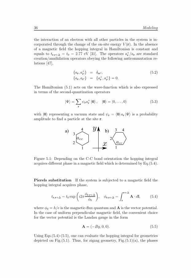
a) b)
1
2
34
1
2
3 4
Figure 5.1: Depending on the C-C bond orientation the hopping integralacquires different phase in a magnetic field which is determined by Eq.(5.4).
Pierels substitution If the system is subjected to a magnetic field thehopping integral acquires phase,
tr,r+∆ = t0 exp
(
i2πφr,r+∆
φ0
)
, φr,r+∆ =
∫r+∆
r
A · dl, (5.4)
where φ0 = h/e is the magnetic-flux quantum and A is the vector potential.In the case of uniform perpendicular magnetic field, the convenient choicefor the vector potential is the Landau gauge in the form
A = (−By, 0, 0). (5.5)
Using Eqs.(5.4)-(5.5), one can evaluate the hopping integral for geometriesdepicted on Fig.(5.1). Thus, for zigzag geometry, Fig.(5.1)(a), the phases

Tigh-binding Hamiltonian and Green’s function 37
are
φ12 =acc
√3
2B
(
y1 +1
4acc
)
; φ21 = −acc√
3
2B
(
y2 −1
4acc
)
;
φ34 = −acc√
3
2B
(
y3 +1
4acc
)
; φ43 =acc
√3
2B
(
y4 −1
4acc
)
;
φ23 = 0; φ32 = 0; (5.6)
and for armchair geometry, Fig.(5.1)(b), we get
φ12 =acc2B
(
y1 +
√3
4acc
)
; φ21 = −acc2B
(
y2 −√
3
4acc
)
;
φ23 = −acc2B
(
y2 +
√3
4acc
)
; φ32 =acc2B
(
y3 −√
3
4acc
)
;
φ34 = −By3acc; φ43 = By4acc; (5.7)
The Green’s function A standard way to define the Green’s functionis [16]
[E −H ± iη]G± = 1 ⇒ G± = [E −H ± iη]−1. (5.8)
where η → 0 is an infinitesimal constant. The sign ± distinguishes betweenretarded (G+) and advanced (G−) Green’s functions. In this chapter onlyretarded Green’s functions are used, therefore we omit the sign thereafter.The Green’s function can also be expressed in terms of eigenvalues andeigenfunctions of the Hamiltonian, H |Ψα〉 = ǫα |Ψα〉,
G(r, r′;E) =∑
α
ψαrψα∗r′
E − ǫα + iη. (5.9)
This equation allows to connect the Green’s function to a local density ofstates (LDOS) which is defined as
ρ(r, E) =∑
α
|ψαr|2δ(E − ǫα). (5.10)
Using the relation
ℑ[
limη→0
1
x + iη
]
= −πδ(x), (5.11)
we finally arrive at the required equation for LDOS
ρ(r, E) = −1
πℑ[
limη→0
G(r, r;E)
]
. (5.12)
Computation of the Green’s function by direct matrix inversion is anextremely time-consuming routine. If the structure consist of M-slices with

38 Modeling
N -sites on each slice, the real-space Hamiltonian matrix has a dimensionNM ×NM , which makes matrix inversion inefficient for structures with asize relevant for experiments. One way to attack the problem is to switchto an energy (or momentum) representation using the Fourier transforma-tion. However this method introduce approximation in the original exactproblem. In the next section we describe the recursive Green’s functiontechnique. This method does not require any simplifications in comparisonwith the original problem and allows to avoid the full Hamiltonian matrixinversion.
5.2 Recursive Green’s function technique:
application to graphene nanoribbons
In this section we use the technique described in Refs. [48, 49] and ap-plied previously to study properties of graphene nanoribbons and photoniccrystals.
5.2.1 Dyson equation
0 1 2 N N+1i
a) b)
Figure 5.2: Schematic illustration showing the application of a) Dysonequation and b) the recursive Green’s function technique.
Imagine that we have two isolated subsystems described by the Hamil-tonians H0
1 and H02 . Then, we put them together and let interact via
potential V [see Fig.(5.2) (a)]. Thus, the total Hamiltonian reads
H = H01 +H0
2︸ ︷︷ ︸
H0
+V = H0 + V. (5.13)
The Green’s function corresponding to this Hamiltonian equals to
G−1 = E −H0
︸ ︷︷ ︸
(G0)−1
−V = (G0)−1 − V. (5.14)

Recursive Green’s function technique 39
Multiplying the above equation on the left by G0 and on the right by G(or vice versa) and rearranging variables, we derive the Dyson equation
G = G0 +G0V G, (5.15)
(G = G0 +GVG0).
The Dyson equation is an extremely useful relation and is a basis of therecursive Green’s function technique. If we define the matrix element asGmn = 〈m|G|n〉, the Dyson equation reads
Gmn = G0mn +
∑
i,j
G0miVijGjn, (5.16)
(Gmn = G0mn +
∑
i,j
GmiVijG0jn).
Hence, attaching two slices with the use of the Dyson equation, the Green’sfunction for the combined system is
G11 = (I −G011V12G
022V21)
−1G011,
G12 = G011V12(I −G0
22V21G011V12)
−1G022,
G21 = G022V21(I −G0
11V12G022V21)
−1G011, (5.17)
G22 = (I −G022V21G
011V12)
−1G022.
Let us now consider a typical structure for transport experiments il-lustrated in Fig. (5.2)(b). It consists of ideal (non scattering) leads anddevice (scattering) region. The first step is to split the device region intoslices {i} describing by relatively simple Hamiltonians H0
i
H =
N∑
i
H0i + U. (5.18)
By ’simple’ we imply the Hamiltonian of a such size, for which the corre-sponding Green’s function can be found by direct matrix inversion G0
ii =[E − H0
i ]−1. The leads are assumed to be uniform, which often allows tofind the surface Green’s function (Γ) analytically or by using the techniquedescribed in Sec.(5.2.4). Thus, having the surface Green’s functions ΓL andΓR and using Dyson Eqs.(5.17), one can add recursively slice by slice to findthe Green’s function of each slice Gii as a part of the whole system, whichprovide information about LDOS, Eq.(5.12); and the Green’s function ofthe device GN+1,0, which allows to calculate transmission coefficient (seeEq.(5.45) in Sec.(5.2.5)).

40 Modeling
5.2.2 Bloch states
Let us consider an infinitely long ideal graphene nanoribbon consisting of Nsites in the transverse j-direction, as illustrated in Fig.(5.3). The structurehas a translational symmetry in i-direction with unit cell consisting ofM = 2 slices for zigzag GNRs and M = 4 in the case of armchair GNRs.
1
2
3
4
5
6
1
2
3
4
5
6
1 2 301
2
3
4
5
6
4
1
2
3
5
6
1
2
3
4
5
6
1
2
3
4
5
6
1 2 3 4 50
armchair graphene nanoribbon
zigzag graphene nanoribbon
zGNR unit cell aGNR unit cell
a)
b)
c) d)
Figure 5.3: a) zigzag and b) armchair graphene nanoribbons and corre-sponding to them unit cells c), d).
The Hamiltonian of the structure can be split into three parts
H = Hcell +Hout + U, (5.19)
where the operators Hcell describes the unit cell spanning slices 1 ≤ i ≤M ,while Hout describes the region including all other slices −∞ < i ≤ 0and M + 1 ≤ i < ∞. The coupling between the cell and slices i = 0 andi = M+1 is described by the hopping operator U . The total wave functionconsists of two parts,
|ψ〉 = |ψcell〉 + |ψout〉, (5.20)
corresponding to the unit cell and outside region respectively. SubstitutingEqs. (5.20), (5.19) into the Schrodinger equation H|ψ〉 = E|ψ〉 and makinguse of definition of the Green’s function (5.8), we obtain
|ψcell〉 = GcellU |ψout〉, (5.21)
where Gcell is the Green’s function of the operator Hcell. This equationallows us to relate the wave-function in the cell (slice i = 1 and i = M)with the wave-function in the outside region (slice i = 0 and i = M + 1).
Recursive Green’s function technique 41
Hence calculating the matrix element ψi,j = 〈0|ai,j|ψ〉, we get
ψ1 = G1,1cellU1,0ψ0 +G1,M
cell U+1,0ψM+1,
ψM = GM,1cell U1,0ψ0 +GM,M
cell U+1,0ψM+1, (5.22)
where we used that UM,M+1 = U0,1 due to the periodicity of the ribbon andU0,1 = U+
1,0. The vector ψi corresponds to the wave-function on a slice i
ψi =
ψi,1...
ψi,N
, (5.23)
and the Green’s function on the cell and the coupling matrices are definedby
(U1,0)jj′ = 〈0|a1,jUa+0,j′|0〉 (5.24)(
Gi,i′
cell
)
jj′= 〈0|ai,jGcella
+i′,j′|0〉.
Equation (5.22) can be rewritten in a compact form
T1
(ψM+1
ψM
)
= T2
(ψ1
ψ0
)
, (5.25)
where
T1 =
(−G1,M
cell U+1,0 0
−GM,Mcell U+
1,0 I
)
, T2 =
(−I G1,1
cellU1,0
0 GM,1cell U1,0
)
(5.26)
and I being the unitary matrix. Since we consider the ideal nanoribbon,the wave-function has the Bloch form with a periodicity equals to the pe-riodicity of the structure,
ψm+M = eikMIψm. (5.27)
This allows to rewrite Eq.(5.25) in the form of an eigenvalue problem
T−11 T2
(ψ1
ψ0
)
= eikM(ψ1
ψ0
)
. (5.28)
For a fixed energy E, solution of (5.28) gives a set of eigenvalues {kα} andeigenfunctions {ψα
0 }, {ψα1 }, 1 ≤ α ≤ 2N . Among 2N states there are Nprop-
propagating states and Nevan-evanescent states, which can be separated bythe value of imaginary part of kα (i.e. |Im[kα]| > 0 for evanescent states).The propagating states, in turn, can be separated into two equal parts,right- and left-propagating states, by calculating their group velocities.This is described in the next section.
42 Modeling
5.2.3 Calculation of the Bloch states velocity
As it is shown in Sec. (5.2.5), in order to calculate the transmission and re-flection coefficients, one needs to know the velocities of propagating states.Moreover, the sing of velocity of Bloch state is used to separated the statesby its direction of propagation, which is required to construct the surfaceGreen’s functions (see Sec. (5.2.4)). In order to calculate the velocity weuse the standard formula for the group velocity
v =1
~
∂E
∂k. (5.29)
One can estimate the derivative by direct numerical differentiation (E(kα2 )−E(kα1 ))/(kα2 −kα1 ). However it’s not efficient since it requires to solve eigen-value problem (5.28) twice. Moreover, each time the eigensolver is called,the eigenvalues are given in different order.
In this section we derive the explicit form of the derivative. The wave-function of the α-th Bloch state within the unit cell is given by
|ψα〉 =
M∑
i=1
|ψαi 〉, |ψα
i 〉 = eikαxi |ϕαi 〉. (5.30)
(Thereafter we omit α to simplify notation.) Making use of the relation〈ψi|H|ψ〉 = E〈ψi|ψ〉 = E|ϕi|2, we obtain
v =1
~
∂E
∂k=
1
~
1
M
M∑
i=1
∂
∂k
[〈ψi|H|ψ〉|ϕi|2
]
, (5.31)
where the elements of the vector
ϕi =
ϕi,1...
ϕi,N
(5.32)
equal to ϕi,j = 〈0|ai,j|ϕ〉. Finally, calculating the matrix element 〈ψi|H|ψ〉with Hamiltonian in the form (5.18), the velocity reads
v = −1
~
i
M
M∑
i=1
ϕ∗Ti|ϕi|2
[
(xi − xi−1)Ui,i−1ϕi−1e−ik(xi−xi−1)
−(xi+1 − xi)Ui,i+1ϕi+1eik(xi+1−xi)
]
. (5.33)
In the case of zero magnetic field, this equation can be simplified for zigzagnanoribbons
v =acc
√3
2~sin k
M=2∑
i=1
ϕ∗Ti−1|ϕi−1|2
Ui−1,iϕi, (5.34)
where we used that ϕi = ϕi+M due to periodicity.
Recursive Green’s function technique 43
5.2.4 Surface Green’s function
Applying the Dyson equation, one can construct the Green’s function ofthe scattering region of an arbitrary shape. However in calculation of trans-port properties of the system, one usually assumes that the system is openand attached to a perfect (non-scattering) semi-infinite leads. Hence, oneis interested in finding the surface Green’s function of the leads as a start-ing point for Dyson equation. Most of the methods for calculation of theGreen’s function rely on searching for a self-consistent solution for ΓR andΓL which makes these calculation very time consuming [50]. The method[48, 49] presented in this section does not require self-consistent calcula-tions, and the surface Greens function is expressed in terms of the Blochstates of the graphene lattice.
Let us consider a semi-infinite periodic ideal graphene ribbon extendedto the right in the region −M ≤ i < ∞. Suppose that an excitation |s〉is applied to its surface slice i = −M . Introducing the Green’s functionof the semi-infinite ribbon, Grib, one can write down the response to theexcitation |s〉 in a standard form [16]
|ψ〉 = Grib|s〉. (5.35)
The unit cell of a graphene lattice spans slices 1 ≤ i ≤ M , (M = 2 and4 for the zigzag and armchair lattices, see Fig. 5.3). Applying the Dysonequation between the slices 0 and 1, we get
G1,−Mrib = ΓRU1,0G
0,−Mrib , (5.36)
where we defined the right surface Green’s function as ΓR ≡ G1,1rib. Evalu-
ating the matrix elements 〈0|a1,j |ψ〉 of Eq. (5.35) and making use of Eq.(5.36), we obtain for each Bloch state α
ψα1 = ΓRU1,0ψ
α0 . (5.37)
This equations can be used to construct ΓR
ΓRU1,0 = Ψ1Ψ−10 , (5.38)
where Ψ1 and Ψ0 are the square matrices composed of the matrix-columnsψα1 and ψα
0 , (1 ≤ α ≤ N), Eq. (5.23), i.e.
Ψ1 = (ψ11, ..., ψ
N1 ); Ψ0 = (ψ1
0, ..., ψN0 ). (5.39)
The expression for the left surface Greens function ΓL can be derivedin a similar fashion
ΓLU+1,0 = ΨMΨ−1M+1, (5.40)
where the matrices ΨM and ΨM+1 are defined in a similar way as Ψ1 andΨ0 above. Note that matrices ΨM and ΨM+1 can be easily obtained fromΨ1 and Ψ0 using the relation (5.25). Note also that in the case of the zeromagnetic field, the right and left surface Greens functions are identical,ΓL = ΓR.
44 Modeling
5.2.5 Transmission and reflection
According to the Landauer formula (2.42), conductance can be expressed interms of the transmission function. In order to calculate the transmissioncoefficient T (E), the system is divided into three regions, namely, twoideal semi-infinite leads of the width N extending in the regions i ≤ 0and i ≥ L respectively, and the central scattering region (device), seeFigs.(5.2),(5.3). The left and right leads are assumed to be identical. Theincoming, transmitted and reflected states in the leads, |ψi
α〉, |ψtα〉 and |ψr
α〉,have the Bloch form,
|ψiα〉 =
∑
i≤0eik
+α xi
N∑
j=1
φαi,j a
+i,j|0〉 (5.41)
|ψtα〉 =
∑
i≥L
∑
β
tβαeik+
β(xi−xL)
N∑
j=1
φβi,j a
+i,j|0〉 (5.42)
|ψrα〉 =
∑
i≤0
∑
β
rβαeik−
βxi
N∑
j=1
φβi,j a
+i,j|0〉, (5.43)
where tβα (rβα) are the transmission (reflection) amplitude from the incom-ing Bloch state α to the transmitted (reflected) Bloch state β (α → β),and we choose x0 = 0. The transmission and reflection coefficients can beexpressed through the corresponding amplitudes and the Bloch velocities[16]
T =∑
α,β
vβvα
|tβα|2; R =∑
α,β
vβvα
|rβα|2. (5.44)
The summation includes only propagating states. For the transmission andreflection amplitudes we use the equations given in Ref. [49],
Φ1T = −GL,0(U0,1Φ1K − ΓL−1Φ0), (5.45)
Φ0R = −G0,0(U0,1Φ1K − ΓL−1Φ0) − Φ0, (5.46)
where the matrices T and R of the dimension N × Nprop and have thefollowing meaning, (T )βα = tβα, (R)βα = rβα; (with Nprop being the numberof propagating modes in the leads); GL,0 and G0,0 are the Green’s functionmatrices and ΓL is the left surface Green’s function, Eq. (5.40); U0,1 couplesthe left lead and the scattering region; K is the diagonal matrix with thematrix elements Kα,β = exp(ik+α x1)δα,β . The square matrices Φ1 and Φ0
are composed of the Bloch states φα0 and φα
1 , Eq.(5.30), on the slices 0 and1 of the ribbon unit cell, i.e. Φ1 = (φ1
1, ..., φN1 ) and Φ0 = (φ1
0, ..., φN0 ).

Real-space Kubo method 45
5.3 Real-space Kubo method
The real-space Kubo method is a powerful tool to study transport proper-ties of a system consisting of several millions of atoms. It was developed byS. Roche and D. Mayou [51, 52] and then applied extensively to investigateproperties of carbon nanotubes [53, 54] and graphene [55, 56, 57]. Themethod is based on numerical solution of the time-dependent Schrodingerequation. Having calculated wave-function at different times, one can com-pute the mean square spreading of a wave packet. This quantity is pro-portional to the diffusion coefficient, which, in turn, can be related to theconductivity. The derivations provided in this section are primarily basedon Refs. [58, 59].
5.3.1 Diffusion coefficient
The starting point of the model is the Kubo-Greenwood formula for con-ductivity (see Chapter 2 for details)
σij(E) =2e2π~
VTr [vxδ(E −H)vxδ(E −H)] , (5.47)
where V is the system volume, vx is a x-component of the velocity operatorand H is the Hamiltonian of the system. The last delta function can bewritten as a Fourier transform
δ(E −H) =1
2π~
∫ +∞
−∞dtei(E−H)t/~. (5.48)
Substituting it in Eq.(5.47), we get
σ(E) = e2∫ +∞
−∞dtTr
[vxδ(E −H)eiEt/~vxe
−iHt/~]. (5.49)
Using the relation eiEt/~ = eiHt/~ and recalling the Heisenberg form ofoperators, vx(t) = eiHt/~vxe
−iHt/~, we arrive
σ(E) = e2∫ +∞
−∞dtTr [vx(0)δ(E −H)vx(t)] . (5.50)
Introducing the velocity autocorrelation function
〈vx(t)vx(0)〉E =Tr [vx(0)δ(E −H)vx(t)]
Tr [δ(E −H)], (5.51)
the equation for conductivity becomes
σ(E) = e2∫ +∞
−∞dtTr [δ(E −H)] 〈vx(t)vx(0)〉E. (5.52)

46 Modeling
It is possible to show that the velocity autocorrelation function 〈vx(t)vx(0)〉can be related to the mean value of the spreading in the x-direction,χ2(E, t) = 〈(x(t) − x(0))2〉E as
d2
dt2χ2(E, t) = 〈vx(t)vx(0)〉E, (5.53)
where x(t) = eiHt/~xe−iHt/~ is the x-component of the position operator inthe Heisenberg picture. Inserting Eq.(5.53) into Eq.(5.52) and performingintegration, we get
σ(E) = e2Tr [δ(E −H)] limt→∞
d
dtχ2(E, t). (5.54)
Using the definition of χ2(E, t), the conductivity reads as
σ(E) = e2Tr [δ(E −H)] limt→∞
d
dt
(Tr [δ(E −H)(x(t) − x(0))2]
Tr [δ(E −H)]
)
= e2Tr [δ(E −H)] limt→∞
d
dt(tD(E, t)), (5.55)
where we have introduce a new quantity called diffusion coefficient anddefined it as
D(E, t) =χ2(E, t)
t=
1
t
Tr [δ(E −H)(x(t) − x(0))2]
Tr [δ(E −H)]=
1
t
nx(E, t)
n(E), (5.56)
where n(E) is a density of states (DOS). Details of calculation of nx(E, t)are given in Sec.(5.3.3).
5.3.2 Transport regimes
The diffusion coefficient, D(E, t), does depend on time. Figure (5.4) il-lustrates typical time-evolution of the diffusion coefficient. Analyzing itsbehavior one can distinguish three transport regimes, namely
1. ballistic
2. diffusive
3. localization
Ballistic regime For times t < τball, when the number of scatteringevents is small, the wave-packet propagates ballistically. This is manifestedby linear growth of the diffusion coefficient as a function of time such that
√
χ(E, t)2 = v(E)t (5.57)
D(E, t) = v(E)2t. (5.58)
If the system is large enough or the impurities concentration ni is high, thediffusion coefficient saturates and becomes constant at time τball ≈ d/v(E),where d =
√ni is an average distance between impurities.

Real-space Kubo method 47
Figure 5.4: Diffusion coefficient as a function of time. Three transportregimes (ballistic, diffusion, localization) are separated by dashed lines.The slope of D is proportional to the square of velocity v2. Dotted linedenotes maximal value of D which corresponds to a semiclassical limit.
Diffusive regime In this regime the diffusion coefficient is independentof time, D(E, t) = D(E). Hence, the conductivity according to Eq.(5.55)becomes
σ(E) = e2ρ(E)D(E), (5.59)
where ρ(E) = n(E)/S is a density of states per unit area per spin and Sis an area of the system. This equation is also known as Einstein relationfor conductivity [16].
In some cases the plateau on the diffusivity plot is small and lineargrowth of D is immediately changed by decay. This is in contrast to theclassical regime where the diffusion coefficient does not change when t →∞. Thus, in order to calculate conductivity in the diffusive regime, Eq.(5.59) is modified such that the maximum value of the diffusion coefficient,D(E, t) → Dmax(E), is used [55]
σsc(E) = e2ρ(E)Dmax(E). (5.60)
This corresponds to a semi-classical conductivity within the Boltzmannapproach where quantum effects leading to localization are not taken intoaccount
σBoltz = e2ρ(E)τv2F2, (5.61)
with τ being a scattering time. Comparing two equations, one can relatethe mean free path to the computed diffusion coefficient
le = vF τ =2Dmax
vF. (5.62)
Localization regime The effect of localization can be viewed as con-structing interference between forward and backward electron trajectories.

48 Modeling
When these effects become dominant, the diffusion coefficient decreases[55, 56]. According to the theory of localization, conductivity decreaseswith the increase of the system length L. In the Kubo approach we canrelate L to time by L =
√
χ(E, t)2. In this case conductivity depends onthe size of the system
σ(E) ∼ exp
(
−L(t)
ξ
)
, (5.63)
with ξ being localization length.
Figure 5.5: Diffusion coefficient as a function of time for different concen-tration of strong short-range impurities [59]. The graphene sample consistsof 6.8 millions of carbon atoms.
Figure (5.5) [59] illustrates the normalized diffusion coefficient calcu-lated for graphene sample consisting of 6.8 millions of carbon atoms. De-pending on the concentration of impurities the system appears to be indifferent transport regimes within plotted time interval. If the impurityconcentration is zero, electrons propagate ballistically and the diffusion co-efficient (blue line) grows linearly. For concentration n = 2% the diffusioncoefficient undergoes crossover from ballistic to diffusive regime (red line)at time t = 20 fs. At n = 5% localization effects becomes dominant alreadyat t = 10 fs which is manifested by the decrease of D (green line) with time.
5.3.3 Time evolution
According to Eq.(5.56), in order to calculate the diffusion coefficient, weneed to compute the quantity
nx(E, t) = Tr[δ(E −H)(x(t) − x(0))2
]. (5.64)
Time-dependence of the position operator can be rewritten in the Heisen-berg picture x(t) = eiHtxe−iHt, which yields
nx(E, t) = Tr[
(eiHtxe−iHt − x)δ(E −H)(eiHtxe−iHt − x)]
. (5.65)

Real-space Kubo method 49
Using the commutation relation [H, e−iHt] = 0, we get
nx(E, t) = Tr[
(eiHtx− xeiHt)δ(E −H)(xe−iHt − e−iHtx)]
= Tr[
[x, U(t)]+δ(E −H)[x, U(t)]]
, (5.66)
where U(t) = e−iHt is a time evolution operator. In order to estimate thetrace we need to know how the operator [x, U(t)] acts on the wave-function|ψi〉, i.e
[x, U(t)]|ψi〉 = x(
U(t)|ψi〉)
−U(t) (x|ψi〉) = x|ψi(t)〉−U(t) (x|ψi〉) . (5.67)
If we denote |ψxi 〉 = x|ψi〉, then
nx(E, t) =∑
i
〈Ψi(t)|δ(E − H)|Ψi(t)〉, (5.68)
where |Ψi(t)〉 = |ψi(t)〉 − |ψxi (t)〉. Mathematically Eq.(5.68) is similar to
equation for finding of the local density of states. The details of LDOScalculation are given in Sec.(5.3.7).
5.3.4 Exact solution of the time-dependent Schrodinger
equation: Chebyshev method
As it is seen from Eq.(5.56) and subsequent discussion in Sec. (5.3.2), thediffusion coefficient is a function of time. In order to estimate D(E, t) atdifferent times t one needs to know the wave-function ψ(t) in accordanceto Eq.(5.68). In this section we present an efficient method for solutionof the time-dependent Schrodinger equation based on the expansion of thetime evolution operator in an orthogonal set of Chebyshev polynomials[51, 58, 57].
The starting point is the time-dependent Schrodinger equation
H |ψ(t)〉 = i~∂
∂t|ψ(t)〉 , (5.69)
with H being the tight-binding time-independent Hamiltonian. If the initialwave-function at time t0, |ψ(t = 0)〉 = |ψ0〉, is known, the formal solution ofEq.(5.69) can be expressed via the time-evolution operator (or propagator)U(t),
|ψ(t)〉 = U(t) |ψ0〉 , U(t) = e−i~H(t). (5.70)
In order to expand U(t) in a set of the Chebyshev polynomials Tn(x) (whichare defined in the interval x ∈ [−1; 1]), we first renormalize the Hamiltoniansuch that its spectrum lies in the above interval,
Hnorm =2H − (Emax + Emin)I
Emax − Emin
, (5.71)

50 Modeling
where Emax and Emin are the largest and the smallest eigenvalues of theoriginal Hamiltonian Eq. (4.6). (In order to calculate Emax and Emin weuse a computational routine that estimates the largest/smallest eigenvaluesof the operator without calculation of all the eigenvalues).
Expanding U(t) in Chebyshev polynomials in Eq. (5.70) we obtain forthe wave function,
|ψ(t)〉 =∞∑
n=0
cn(t) |Φn〉 , (5.72)
where the functions |Φn〉 = Tn(Hnorm) |ψ0〉 are calculated using the recur-rence relations for the Chebyshev polynomials,
|Φ0〉 = T0(Hnorm) |ψ0〉 = |ψ0〉 (5.73)
|Φ1〉 = T1(Hnorm) |ψ0〉 = Hnorm |ψ0〉 (5.74)
|Φn+1〉 = Tn+1(Hnorm) |ψ0〉 = 2Hnorm |Φn〉 − |Φn−1〉 . (5.75)
The recursive routine is repeated until the expansion (5.72) converges whichis defined by the condition
∣∣∣∣∣‖
N∑
n=0
cn(t) |Φn〉 ‖ − 1
∣∣∣∣∣< ǫ, (5.76)
where ǫ is some predefined computational tolerance. The expansion coeffi-cients cn(t) are calculated making use of the orthogonality relation for theChebyshev polynomials
cn(t) = 2e−i(Emax+Emin)t
2~ (−i)nJn(Emax − Emin
2~t
)
. (5.77)
For large t the expansion coefficients cn(t) become exponentially small.This leads to the fast convergence of the expansion series Eq. (5.72), andmakes the Chebyshev method very efficient for calculation of the temporaldynamics.
Figure (5.6) illustrates temporal dynamics of a wave-packet in a pure(undoped) graphene. The wave-paket, originally (at t = 0) localized ata single site in the middle of the structure, distributes uniformly in alldirections. Less than 1000 iterations is required to achieve convergence for80 fs of elapsed time.

Real-space Kubo method 51
Figure 5.6: Temporal dynamics of the wave-packet in 2D graphene. Atinitial time the wave-packe was localized at a single site in the middle ofthe structure.
5.3.5 Continued fraction technique
Consider a Hamiltonian matrix given in a tridiagonal form,
Htri =
α1 β1 0 · · · · · · · · · · · ·β1 α2 β2 0 · · · · · · · · ·0 β2 α3 β3 0 · · · · · ·... 0 β3
. . .. . .
. . . · · ·...
... 0. . .
. . .. . .
. . ....
......
. . .. . .
. . . βN−1...
......
.... . . βN−1 αN
. (5.78)
Our aim is to calculate the first diagonal element G11 of the Greens functionG = (EI − Htri)
−1 without a computing the whole Greens function and allthe eigenvalues/eigenfunctions of the Hamiltonian.
Let us denote λi = G1i. From the definition of the Greens function weobtain [60],
(E − αi)λi − βi−1λi−1 − βiλi+1 = 0, 2 ≤ i ≤ N − 1 (5.79)
with (E − αN)λN − βN−1λN−1 = 0 and (E − α1)λ1 − β1λ2 = 1. Expressingsequentially λN by λN−1, λN−1 via λN−2 and λN−3 we express G11 as acontinued fraction [58, 59, 60, 61]:
G11 =1
E − α1 −β21
E − α2 −β22
E − α3 − β23
...
. (5.80)
Even for a huge matrices calculation of G11 does not require a lot ofcomputational time. However if the Hamiltonian matrix is given in a gen-eral form, i.e. consist of arbitrary number of diagonals, it must be first
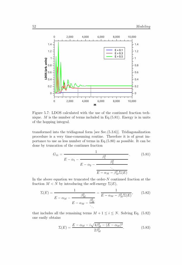
52 Modeling
Figure 5.7: LDOS calculated with the use of the continued fraction tech-nique. M is the number of terms included in Eq.(5.81). Energy is in unitsof the hopping integral.
transformed into the tridiagonal form [see Sec.(5.3.6)]. Tridiagonalizationprocedure is a very time-consuming routine. Therefore it is of great im-portance to use as less number of terms in Eq.(5.80) as possible. It can bedone by truncation of the continues fraction
G11 =1
E − α1 −β21
E − α2 −β22
...E − αM − β2
MΣ(E)
. (5.81)
In the above equation we truncated the order-N continued fraction at thefraction M < N by introducing the self-energy Σ(E),
Σ(E) =1
E − αM − β2M
E − αM − β2M
. . .
=1
E − αM − β2MΣ(E)
, (5.82)
that includes all the remaining terms M + 1 ≤ i ≤ N . Solving Eq. (5.82)one easily obtains
Σ(E) =E − αM − i
√
4β2M − (E − αM)2
2β2M
. (5.83)
Real-space Kubo method 53
The number of terms M included in the summation in Eq. (5.81) is de-termined from the condition for the convergence of G11. As it is seen fromFig.(5.7), the higher energy the more elements should be included in thesummation. For this particular case (N = 10000), half of the elements isenough to achieve high accuracy of calculations in a broad energy interval.
5.3.6 Tridiagonalization of the Hamiltonian matrix
In the real-space representation the tridiagonal Hamiltonian, which is givenby Eq.(5.78), usually corresponds to a one-dimensional chain with nearest-neighbor interaction. In practice, however, Hamiltonian has more com-picated form. For instance, for 2D graphene it can consist of up to 9diagonals if the periodic boundary conditions are used. In order to utilizethe continued fraction technique to calculate G11 the Hamiltonian shouldbe first transformed to the tridiagonalized form H → Htri. This is doneby constructing a new orthogonal basis as described below. We start byselecting the first basis vector |1}. Curled brackets |i} are used to denotethe new basis vectors while straight brackets |i〉 denote the old ones. Ifthe tridiagolization is performed in order to find the local density if stateson the i-th site of the system at hand, the first basis vector is selected as|1} = |i〉, where |i〉 = c†i |0〉.
We require that the Hamiltonian in the new basis be of the tridiagonalform (5.78). By operating H|i} we arrive to the following equations [58,59, 60],
H|1} = α1|1} + β1|2}, (5.84)
H|i} = βi−1|i− 1} + αi|i} + βi|i+ 1}, 2 ≤ i ≤ N − 2, (5.85)
H|N} = βN−1|N − 1} + αN |N}. (5.86)
Using Eq. (5.84) and the orthogonality relation {1|2} = 0 we obtain thesecond basis vector and the matrix elements α1 and β1,
|2} =1√C2
(
H|1} − α1|1})
, (5.87)
α1 = {1|H|1}, β1 = {2|H|1},
where the normalization coefficient C2 (as well as all other normalizationcoefficients Ci, 2 ≤ i ≤ N) are obtained from the normalization requirement{i|i} = 1.
We then proceed to Eq. (5.85) and recursively calculate the basis vec-tors |i}, 2 ≤ i ≤ N − 2, and corresponding matrix elements αi and βi,
|i+ 1} =1√Ci+1
(
H|i} − βi−1|i− 1} − αi|i})
, (5.88)
αi = {i|H|i}, βi+1 = {i+ 1|H|1}, 2 ≤ i ≤ N − 2.

54 Modeling
Finally, from Eq. (5.86) we obtain
|N} =1√CN
(
H|N} − αN |N})
, αN = {N |H|N}, (5.89)
which concludes the tridiagonalization procedure.
5.3.7 Local density of states
The techniques describe in the previous sections, namely tridiagolizationand continued fraction technique, provides an efficient way to calculate thelocal density of states (LDOS). If the system is described by the real-spaceHamiltonian H given in the matrix form, LDOS at site i can be calculatedby (see Eq.(5.12) in Sec.(5.1))
ρi(E) = −1
πℑ[
limη→0
Gii(E + iη)
]
, G(E) = (EI −H)−1. (5.90)
In order to calculate Gii, the Hamiltonian must be first tridiagonalized. Thefirst basis vector is chosen in a such way that all elements except i-th areequal to zero, hence |1} = |i〉. Then, then the continued fraction techniqueis applied to calculate G11(E), which in the new basis corresponds to therequired Gii(E).
If one needs to compute DOS, it can be done by calculating LDOSon each site and then averaged over them. However this is not an efficientway, since the Hamiltonian must be tridiagonalized for each site separately.Instead we generate a random state, which extends over M-sites in themiddle of the structure,
|ψran〉 =1√M
∑
i
e2iπαi |i〉, (5.91)
and choose the first basis vector as |1} = |ψran〉. Then the Hamiltonian istridiagonalized as described in Sec.(5.3.6) and LDOS computed by ρi(E) =− 1
πℑ [limη→0Gii(E + iη)] using the continues fraction technique. In this
new basis one ’site’ corresponds to the chosen domain consisting of M realsites. Therefore calculating LDOS we obtain DOS.
Chapter 6
Summary of the papers
6.1 Paper I
In this paper we consider a system consisting of the graphene nanoribbonlocated on an insulating substrate with a metallic back used to tune chargedensity. We develop an analytical theory for the gate electrostatics of theGNRs and calculate the capacitance. The total capacitance of the system isa sum of two contributions: the classical capacitance which is determined bythe geometry of the system and a dielectric permittivity and the quantumcapacitance which arises from a finite density of state of the GNR. Tocomplement our study we also perform numerical calculations which arebased on the tight-binding Hamiltonian. The effect of electron-electroninteraction is taken into account within the Hartree approximation. Fora chosen gate voltage the charge density is calculated self-consistently byintegrating LDOS which is computed using the recursive Green’s functiontechnique.
We show that the distribution of charge density and potential is notuniform. Due to the electrostatic repulsion electrons tend to accumulatenear the boundaries. It is also demonstrated that electron-electron inter-action leads to significant modification of the band structure. Our exactnumerical calculations show that the density distribution and the potentialprofile in the GNRs are qualitatively different from those in conventionalsplit-gate quantum wires with a smooth electrostatic confinement wherethe potential is rather flat and the electron density is constant throughoutthe wire. At the same time, the electron distribution and the potentialprofile in the GNR are very similar to those in the cleaved-edge overgrownquantum wires (CEOQW) exhibiting triangular-shaped quantum wells inthe vicinity of the wire boundaries. This similarity reflects the fact thatboth the CEOQWs and the GNRs correspond to the case of the hard-wallconfinement at the edges of the structure.

56 Summary of the papers
6.2 Paper II
We study interaction and screening effects in a gated bilayer graphenenanoribbon. We employ the numerical model similar to the model de-scribed in paper I in order to study electron distribution and the energygap in bGNRs. We also derive an analytical expression for a dependence ofa potential difference between graphene layers and the gate voltage. Theanalytical estimations are shown to be in a good quantitative agreementwith the numerical calculations. We demonstrate, see Fig.(6.1), that in
0 5 10 15 20 25 300
20
40
60
80
100
d=15 nm
d=50 nm d=100 nm
V (V)
E
(m
eV)
0.5
0.54
0.58
0.62
0.87
0.91
0.95
0.99
0 0.04 0.08-0.04-0.080 0.04 0.08-0.04-0.08
E (
)γ
0
1 2
3
5
(b)
(a)
E (
)γ
0E
(
)
γ0
g
g
k (1/a)
6
8.5
8.6
8.7
0-0.1-0.2 0.1 0.2-0.1-0.2 0 0.20.1
k (1/a)
4.3
4.4
4.5
4
1.92
1.96
2
2.04
2.08
2.12
-0.1-0.15 0 0.150.1-0.05 0.05-0.1 -0.05 0 0.05 0.1
1.32
1.36
1.4
1.44
1.48EF
EFEF
EF
EF EF
1
2
3 4
5
6
Figure 6.1: (a) The energy gap as a function of the applied gate voltagefor various dielectric thicknesses d. (b) Representative band structurescorresponding to the Fermi energies shown in (a). The dashed lines indicatethe positions of Fermi energy.
contrast to 2D graphene sheets the energy gap of the bGNRs dependencenonlinearly on the applied gate voltage. Also the energy gap can collapseat some intermediate gate voltages which is explained by the strong modifi-cation of the energy spectrum caused by the electron-electron interactions.

Paper III 57
6.3 Paper III
Conductance quantization is a hallmark of mesoscopic physics. The firstexperimental observation of the conductance plateau was done more than20 years ago [62]. In magnetic field conductance plateau in a quantum pointcontact becomes more clearly defined, which is attributed to formation ofthe robust edge states. In this paper we investigate the conductance ofgated graphene nanoribbons in a perpendicular magnetic field. We adoptthe recursive Green’s function technique to calculate the transmission co-efficient which is then used to compute the conductance according to theLandauer approach.
10
8
6
4
2
014121086420
(a)
(b)
(c)
(d)
filling factor
G (
2e
/h)
2
B
gate
dielectric
nanoribbon
d
w
w
lB
_ ~~ 11
20 K
50 K
Hartree
Hartreeone-electron
one-electron
Figure 6.2: Conductance of the GNR as a function of filling factor forinteracting and noninteracting electrons at temperatures T = 20 K (redthick lines) and 50 K (blue thin lines) in a magnetic field B = 30 T. Inset:sketch of the sample geometry.
Figure (6.2) shows the conductance as a function of filling factor at afixed magnetic field. We compare both the case of interacting particles cal-culated within the Hartree approximation (solid lines) and the one-electroncase (dashed lines). In the one-electron case the conductance is quantizedas it is expected for ideal (without disorder) GNRs. However in the in-teracting case the conductance quantization is destroyed. This surprisingbehavior is related to the modification of the band structure of the GNRdue to the electron interaction leading, in particular, to the formation ofcompressible strips in the middle of the ribbon and existence of counter-propagating states in the same half of the GNR.
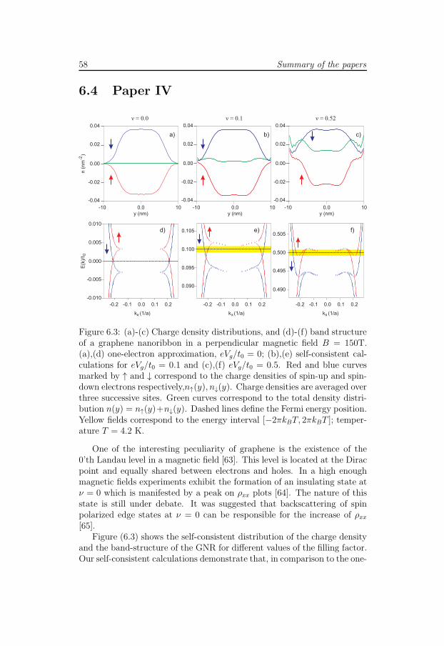
58 Summary of the papers
6.4 Paper IV
-0.010
-0.005
0.000
0.005
0.010
d)
a)
0.105
0.100
0.095
0.090
e)
b)
0.505
0.500
0.495
0.490
-0.2 -0.1 0.0 0.1 0.2 -0.2 -0.1 0.0 0.1 0.2 -0.2 -0.1 0.0 0.1 0.2
f)
c)
k (1/a)k (1/a)k (1/a)
-0.04
-0.02
0.00
0.02
0.04
-0.04
-0.02
0.00
0.02
0.04
-0.04
-0.02
0.00
0.02
0.04
-10 0.0 10
y (nm)
-10 0.0 10
y (nm)
-10 0.0 10
y (nm)
n (
nm
)
-2
x x x
ν = 0.0 ν = 0.1 ν = 0.52
E(k
)/t 0
Figure 6.3: (a)-(c) Charge density distributions, and (d)-(f) band structureof a graphene nanoribbon in a perpendicular magnetic field B = 150T.(a),(d) one-electron approximation, eVg/t0 = 0; (b),(e) self-consistent cal-culations for eVg/t0 = 0.1 and (c),(f) eVg/t0 = 0.5. Red and blue curvesmarked by ↑ and ↓ correspond to the charge densities of spin-up and spin-down electrons respectively,n↑(y), n↓(y). Charge densities are averaged overthree successive sites. Green curves correspond to the total density distri-bution n(y) = n↑(y)+n↓(y). Dashed lines define the Fermi energy position.Yellow fields correspond to the energy interval [−2πkBT, 2πkBT ]; temper-ature T = 4.2 K.
One of the interesting peculiarity of graphene is the existence of the0’th Landau level in a magnetic field [63]. This level is located at the Diracpoint and equally shared between electrons and holes. In a high enoughmagnetic fields experiments exhibit the formation of an insulating state atν = 0 which is manifested by a peak on ρxx plots [64]. The nature of thisstate is still under debate. It was suggested that backscattering of spinpolarized edge states at ν = 0 can be responsible for the increase of ρxx[65].
Figure (6.3) shows the self-consistent distribution of the charge densityand the band-structure of the GNR for different values of the filling factor.Our self-consistent calculations demonstrate that, in comparison to the one-

Paper V 59
electron picture, electron-electron interaction leads to the drastic changesin the dispersion relation and structure of the propagating states in theregime of the lowest LL such as a formation of the compressible strip andopening of additional conductive channels in the middle of the ribbon. Alsowe study the effect of different types of disorder (short-range impurities,edge disorder, warping and spin-flipping) on GNRs conductance, focusingon the robustness of, respectively, edge and bulk state transmissions. Thelatter are shown to be very sensitive to the disorder and get scattered evenif the concentration of the disorder is moderate. In contrast, the edge statesare very robust and cannot be suppressed even in the presence of the strongspin-flipping.
6.5 Paper V
Recent experiments address the effect of correlation in the spatial distri-bution of disorder on the conductivity of graphene sheet by doping it withpotassium atoms. It has been found that the conductivity of the system athand increases as the temperature rises, and argued that this was causedby the enhancement of correlation between the potassium ions due to theCoulomb repulsion [66]. In paper V using the efficient time-dependentreal-space Kubo formalism, we performed numerical studies of conductivityof large graphene sheets with random and correlated distribution of disor-der. In order to describe realistic disorder, we used models of the short-range scattering potential (appropriate for adatoms covalently bound tographene) and the long-range Gaussian potential (appropriate for screenedcharged impurities on graphene and/or dielectric surface). The calcula-tions for the uncorrelated potentials are compared to the correspondingpredictions based on the semiclassical Boltzmann approach and to exactnumerical calculations performed by different methods. We find that forthe most important experimentally relevant cases of disorder, namely, thestrong short-range potential and the long-range Gaussian potential, thecorrelation in the distribution of disorder does not affect the conductivityof the graphene sheets as compared to the case when disorder is distributedrandomly. Our results strongly indicate that the temperature enhancementof the conductivity reported in the recent study [66] and attributed to theeffect of dopant correlations was most likely caused by other factors notrelated to the correlations in the scattering potential.
6.6 Paper VI
The value of a spin-splitting caused by the Zeeman effect is proportionalto the g-factor. For graphene the g-factor equals to its free-electron value
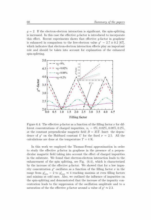
60 Summary of the papers
g = 2. If the electron-electron interaction is significant, the spin-splittingis increased. In this case the effective g-factor is introduced to incorporatethis effect. Recent experiments shows that effective g-factor in grapheneis enhanced in comparison to the free-electron value g∗ = 2.7 ± 0.2 [67],which indicates that electron-electron interaction effects play an importantrole and should be taken into account for explanation of the enhancedspin-splitting.
Figure 6.4: The effective g-factor as a function of the filling factor ν for dif-ferent concentrations of charged impurities, ni = 0%, 0.02%, 0.08%, 0.2%,at the constant perpendicular magnetic field B = 35T. Inset: the depen-dence of g∗ on the Hubbard constant U for the fixed ν = 2.5. All thecalculations are done at the temperature T = 4 K.
In this work we employed the Thomas-Fermi approximation in orderto study the effective g-factor in graphene in the presence of a perpen-dicular magnetic field taking into account the effect of charged impuritiesin the substrate. We found that electron-electron interaction leads to theenhancement of the spin splitting, see Fig. (6.4), which is characterizedby the increase of the effective g-factor. We showed that for a low impu-rity concentration g∗ oscillates as a function of the filling factor ν in therange from g∗min = 2 to g∗max ≈ 4 reaching maxima at even filling factorsand minima at odd ones. Also, we outlined the influence of impurities onthe spin-splitting and demonstrated that the increase of the impurity con-centration leads to the suppression of the oscillation amplitude and to asaturation of the the effective g-factor around a value of g∗ ≈ 2.3.

Bibliography
[1] K. S. Novoselov, A. K. Geim, S. V. Morozov, D. Jiang, Y. Zhang, S.V. Dubonos, I. V. Grigorieva, and A. A. Firsov, Electric field effect inatomically thin carbon films, Science 306, 666 (2004).
[2] P. R. Wallace, The band theory of graphite, Physical Review 71, 622(1947).
[3] K. Wakabayashi, M. Fujita, H. Aijiki, and M. Sigrist, Electronic andmagnetic properties of nanographite ribbons, Phys. Rev. B 59, 8271(1999).
[4] A. K. Geim and K. S. Novoselov, The rise of graphene, Nat. Mat. 6,183 (2007).
[5] A. Barth and W. Marx, Graphene - A rising star in view of sciento-metrics, arXiv:0808.3320v3 [physics.soc-ph] (2008).
[6] M. I. Katsnelson, K. S. Novoselov, and A. K. Geim, Chiral tunnellingand the Klein paradox in graphene, Nat. Phys. 2, 620 (2006).
[7] Y. Zhang , J. W. Tan, H. L. Stormer, and P. Kim, Experimentalobservation of the quantum Hall effect and Berrys phase in grapheneNature 438, 201 (2005).
[8] X. Du, I. Skachko, F. Duerr, A. Luican, and E. Y. Andrei, Frac-tional quantum Hall effect and insulating phase of Dirac electrons ingraphene, Nature 462, 192 (2009).
[9] F. Schwierz, Graphene transistors, Nat. Nanotech. 5, 487 (2010).
[10] L. Liao, Y.-C. Lin, M. Bao, R. Cheng, J. Bai, Y. Liu, Y. Qu, K. L.Wang, Y. Huang, andX. Duan, High-speed graphene transistors with aself-aligned nanowire gate, Nature 467, 305 (2010).
[11] S. Bae, H. Kim, Y. Lee, X. Xu, J.-S. Park, Y. Zheng, J. Balakrishnan,T. Lei, H. R. Kim, Y. I. Song, Y.-J. Kim, K. S. Kim, B. Ozyilmaz,

62 Bibliography
J.-H. Ahn, B. H. Hong, and S. Iijima, Roll-to-roll production of 30-inch graphene films for transparent electrodes. Nat. Nanotech. 5, 574(2010).
[12] G. Konstantatos, M. Badioli, L. Gaudreau, J. Osmond, M. Bernechea,F. P. G. de Arquer, F. Gatti, and F. H. L. Koppens, Hybrid graphene-quantum dot phototransistors with ultrahigh gain, Nat. Nanotech. 7,363 (2012).
[13] M. Di Ventra, Electrical transport in nanoscale systems, CambridgeUniversity Press (2008).
[14] O. Madelung, Introduction to solid state theory, Springer (1978).
[15] D. K. Ferry, S. M. Goodnick, Transport in nanostructures, Cambridgeuniversity press (1997).
[16] S. Datta, Electronic transport in mesoscopic systems, Cambridge uni-versity press (1997).
[17] D. S. Fisher and P. A. Lee, Relation between conductivity and trans-mission matrix, Phys. Rev. B 23, 6851 (1981).
[18] G. F. Giuliani, and G. Vignale, Quantum theory of the electron liquid,Cambridge university press (2005).
[19] P. Hohenberg, W. Kohn, Inhomogeneous electron gas, Phys. Rev. 136,B864 (1964).
[20] W. Kohn and L. J. Sham, Self-consistent equations including exchangeand correlation effects, Phys. Rev. 140, A1133 (1965).
[21] R. G. Parr, W. Yang Density-Functional Theory of Atoms andMolecules, Oxford University Press (1994).
[22] J. P. Perdew, K. Burke, and M. Ernzerhof, Generalized gradient ap-proximation made simple, Phys. Rev. Lett. 77, 3865 (1996).
[23] K. Lier, R. R. Gerhardts, Self-consistent calculations of edge channelsin laterally confined two-dimensional electron systems, Phys. Rev. B50, 7757 (1994).
[24] Oh, R. R. Gerhardts, Self-consistent Thomas-Fermi calculation of po-tential and current distributions in a two-dimensional Hall bar geom-etry, Phys. Rev. B 56, 13519 (1997).
[25] W.-R. Hannes, M. Jonson, and M. Titov, Electron-hole asymmetry intwo-terminal graphene devices, Phys. Rev. B 84, 045414 (2011).

Bibliography 63
[26] Shaffique Adam, E. H. Hwang, V. M. Galitski, and S. Das Sarma, Aself-consistent theory for graphene transport, Proc. Nat. Acad. of Sci.104, 18392 (2007).
[27] Q. Li, E. H. Hwang, E. Rossi, and S. Das Sarma, Theory of 2D trans-port in graphene for correlated disorder, Phys. Rev. Lett. 107, 156601(2011).
[28] T. Andrijauskas, A. A. Shylau, I. V. Zozoulenko, Thomas-Fermi andPoisson modeling of the gate electrostatics in grapehene nanoribbon,Lith. J. of Phys. 52, 63 (2012).
[29] J. Hubbard, Electron correlations in narrow energy bands, Proc. Roy.Soc. 276, 238 (1963).
[30] E. H. Lieb and F. Y. Wu, Absence of Mott Transition in an Exact So-lution of the Short-Range, One-Band Model in One Dimension, Phys.Rev. Lett. 20, 1445 (1968).
[31] A. H. Castro Neto, F. Guinea, N. M. R. Peres, K. S. Novoselov, andA. K. Geim, The electronic properties of graphene, Rev. Mod. Phys.81, 109 (2009).
[32] G. W. Semenoff, Condensed-matter simulation of a three-dimensionalanomaly, Phys. Rev. Lett. 53, 2449 (1984).
[33] N. W. Ashcroft and N. D. Mermin, Solid state physics, Brooks Cole(1976).
[34] Tsuneya Ando, Theory of electronic states and transport in carbonnanotubes, J. Phys. Soc. of Japan 74, 777 (2005).
[35] D. P. DiVincenzo and E. J. Mele, Self-consistent effective-mass the-ory for intralayer screening in graphite intercalation compounds, Phys.Rev. B 29, 1685 (2007).
[36] M. I. Katsnelson, Graphene: carbon in two dimensions, CambridgeUniversity Press (2012).
[37] L. Brey and H. A. Fertig, Electronic states of graphene nanoribbonsstudied with the Dirac equation, Phys. Rev. B 73, 235411 (2006).
[38] A. Fasolino, J. H. Los, M. I. Katsnelson, Intrinsic ripples in graphene,Nature materials 6, 858 (2007).
64 Bibliography
[39] J. W. Klos, A. A. Shylau, I. V. Zozoulenko, Hengyi Xu, T. Heinzel,Transition from ballistic to diffusive behavior of graphene ribbons in thepresence of warping and charged impurities, Phys. Rev. B 80, 245432(2009).
[40] V. Geringer, M. Liebmann, T. Echtermeyer, S. Runte, M. Schmidt, R.Ruckamp, M. C. Lemme, and M. Morgenstern, Intrinsic and extrin-sic corrugation of monolayer graphene deposited on SiO2, Phys. Rev.Lett. 102, 076102 (2009).
[41] J.C. Meyer, A.K. Geim, M.I. Katsnelson, K.S. Novoselov, D. Obergfell,S. Roth, C. Girit, A. Zettl, On the roughness of single- and bi-layer graphene membranes, Solid State Communications, 143, 101109(2007).
[42] M. Gibertini, A. Tomadin, F. Guinea, M. I. Katsnelson, and M. Polini,Electron-hole puddles in the absence of charged impurities, Phys. Rev.B 85, 201405(R) (2012).
[43] E. McCann, Asymmetry gap in the electronic band structure of bilayergraphene, Phys. Rev. B 74, 161403(R) (2006).
[44] J. Nilsson, A. H. Castro Neto, F. Guinea, and N. M. R. Peres, Trans-mission through a biased graphene bilayer barrier, Phys. Rev. B 76,165416 (2007).
[45] K. S. Novoselov, A. K. Geim, S. V. Morozov, D. Jiang, M. I. Kat-snelson, I. V. Grigorieva, S. V. Dubonos, and A. A. Firsov, Two-dimensional gas of massless Dirac fermions in graphene, Nature (Lon-don) 438, 197 (2005).
[46] Y. Zhang, Y.-W. Tan, H. L. Stormer, and P. Kim, Experimental ob-servation of the quantum Hall effect and Berry’s phase in graphene,Nature (London) 438, 201 (2005).
[47] A. L. Fetter, J. D. Walecka, Quantum theory of many-particle systems,Dover (2003).
[48] H. Xu, T. Heinzel, M. Evaldsson, and I. V. Zozoulenko, Magneticbarriers in graphene nanoribbons, Phys. Rev. B 77, 245401 (2008).
[49] A. I. Rahachou, I. V. Zozoulenko, Light propagation in finite and infi-nite photonic crystals: The recursive Green’s function technique, Phys.Rev. B 72, 155117 (2005).
[50] F. Munoz-Rojas, D. Jacob, J. Fernandez-Rossier, and J. J. Palacios,Coherent transport in graphene nanoconstrictions, Phys. Rev. B 74,195417 (2006).

Bibliography 65
[51] S. Roche and D. Mayou, Conductivity of quasiperiodic systems: a nu-merical study, Phys. Rev. Lett. 79, 2518 (1997).
[52] S. Roche, Quantum transport by means of O(N) real-space methods,Phys. Rev. B 59, 2284 (1999).
[53] S. Roche and R. Saito, Effects of magnetic field and disorder onthe electronic properties of carbon nanotubes, Phys. Rev. B 59, 5242(1999).
[54] S. Roche and R. Saito, Magnetoresistance of Carbon Nanotubes: FromMolecular to Mesoscopic Fingerprints, Phys. Rev. Lett., 87, 246803(2001).
[55] N. Leconte, A. Lherbier, F. Varchon, P. Ordejon, S. Roche, and J.-C.Charlier, Quantum transport in chemically modified two-dimensionalgraphene: From minimal conductivity to Anderson localization, Phys.Rev. B 84, 235420 (2011).
[56] A. Lherbier, S. M.-M. Dubois, X. Declerck, Y.-M. Niquet, S. Roche,and J.-Ch. Charlier, Transport properties of 2D graphene containingstructural defects, arXiv:1204.4574v1 [cond-mat.mes-hall].
[57] S. Yuan, H. D. Raedt, M. I. Katsnelson, Modeling electronic structureand transport properties of graphene with resonant scattering centers,Phys. Rev. B 82, 115448 (2010).
[58] T. Markussen, Quantum transport calculations using wave functionpropagation and the Kubo formula, Master thesis, Technical universityof Denmark (2006).
[59] T. M. Radchenko, A. A. Shylau, and I. V. Zozoulenko, Influence of cor-related impurities on conductivity of graphene sheets: Time-dependentreal-space Kubo approach, Phys. Rev. B 86, 035418 (2012).
[60] S. V. Uzdin, On the calculation of the magnetic structure of surfaces,near-surface layers, and interfaces of 3d metals, Physics of the solidstate Vol. 51, Number 6 (2009).
[61] P. Lambin, J.-P. Gaspard, Continued-fraction technique for tight-binding systems. A generalized-moments method, Phys. Rev. B 26,4356 (1992).
[62] B. J. van Wees, H. van Houten, C. W. J. Beenakker, J. G. Williamson,L. P. Kouwenhoven, D. van der Marel, and C. T. Foxon, Quantizedconductance of point contacts in a two-dimensional electron gas, Phys.Rev. Lett. 60, 848850 (1988).

66 Bibliography
[63] M. O. Goerbig, Electronic properties of graphene in a strong magneticfield, Rev. Mod. Phys. 83, 1193 (2011).
[64] L. Zhang, Y. Zhang, M. Khodas, T. Valla, and I. A. Zaliznyak, Metalto insulator transition on the N=0 Landau level in graphene, Phys.Rev. Lett. 105, 046804 (2010).
[65] D. A. Abanin, K. S. Novoselov, U. Zeitler, P. A. Lee, A. K. Geim,and L. S. Levitov, Dissipative quantum Hall effect in graphene nearthe Dirac point, Phys. Rev. Lett. 98, 196806 (2007).
[66] J. Yan and M. S. Fuhrer, Correlated charged impurity scattering ingraphene, Phys. Rev. Lett. 107, 206601 (2011).
[67] E. V. Kurganova, H. J. van Elferen, A. McCollam, L. A. Ponomarenko,K. S. Novoselov, A. Veligura, B. J. van Wees, J. C. Maan, and U.Zeitler, Spin splitting in graphene studied by means of tilted magnetic-field experiments, Phys. Rev. B 84, 121407, (2011).