electron systems by jiawei xu bs in chemistry, university of science and
TRANSCRIPT

QUANTUM MONTE CARLO STUDY OF WEAKLY INTERACTING MANY-
ELECTRON SYSTEMS
by
Jiawei Xu
B.S. in Chemistry, University of Science and Technology of China, 2002
M.S. in Chemistry, University of Science and Technology of China, 2002
Submitted to the Graduate Faculty of
the Dietrich School of Art and Science in partial fulfillment
of the requirements for the degree of
Doctor of Philosophy in Physical Chemistry
University of Pittsburgh
2012

ii
UNIVERSITY OF PITTSBURGH
THE DIETRICH SCHOOL OF ART AND SCIENCE
This dissertation was presented
by
Jiawei Xu
It was defended on
August 03, 2012
and approved by
Kenneth Jordan, PhD, Distinguished Professor
Karl Johnson, PhD, Professor
Lillian Chong, PhD, Associate Professor
Haitao Liu, PhD, Assistant Professor
Dissertation Advisor: Kenneth Jordan, PhD, Distinguished Professor

iii
Copyright © by Jiawei Xu
2012

iv
Quantum Monte Carlo (QMC) methods are playing an increasingly important role for providing
benchmark results for testing more approximate electronic structure and force field methods.
Two particular variants of QMC, the variational Monte Carlo (VMC) and diffusion Monte Carlo
(DMC) methods, have been applied to study the many-electron systems. All-electron
calculations using QMC methods are performed to study the ground-state energy of the Be atom
with single-determinant and multi-determinant trial functions, the binding energy of the water
dimer, and the binding energy of the water-benzene complex. All of the DMC results achieve
good agreement with high level ab initio methods and experiments. The QMC method with
pseudopotentials is used to calculate the electron binding energies of two forms of (H2O)6. It is
found that the DMC method, when using either Hartree-Fock or density functional theory trial
functions, gives electron binding energies in excellent agreement with the results of large basis
set CCSD(T) calculations. Pseudopotential QMC methods are also used to study the interactions
of the water-benzene, water-anthracene, and water-coronene complexes. The dissociation
energies of water-acene complexes of the DMC calculations agree with several other high level
quantum calculations. Localized orbitals represented as spline functions are used to reduce the
computational cost of the calculations for larger water-acene complexes. The prospects of using
this approach to determine the interaction energy between water and graphite are discussed. In
addition, we introduce correlation-consistent Gaussian-type orbital basis sets for use with the
QUANTUM MONTE CARLO STUDY OF WEAKLY INTERACTING MANY-
ELECTRON SYSTEMS
Jiawei Xu, PhD
University of Pittsburgh, 2012

v
Casino Dirac-Fock pseudopotentials. These basis sets give low variances in VMC calculations
and lead to significantly improved convergence compared to non-optimized basis sets in DMC
calculations. We also examine the performance of two methods, the locality approximation (LA)
and T-move, that have been designed for dealing with the problems associated with the use of
non-local pseudopotentials in quantum Monte Carlo calculations. The two approaches give
binding energies of water dimer that agree within the statistical errors. However, the
convergence behavior of the DMC calculations is better behaved when using the T-move
approach.

vi
TABLE OF CONTENTS
PREFACE ................................................................................................................................. XIII
1.0 INTRODUCTION ........................................................................................................ 1
2.0 THE QUANTUM MONTE CARLO METHOD ...................................................... 7
2.1 INTRODUCTION ............................................................................................... 7
2.2 THE METROPOLIS ALGORITHM ................................................................ 8
2.3 VARIATIONAL MONTE CARLO ................................................................. 11
2.4 DIFFUSION MONTE CARLO ........................................................................ 14
2.4.1 Introduction ................................................................................................... 14
2.4.2 The Green’s Function Propagator ............................................................... 15
2.4.3 The Short Time Approximation ................................................................... 16
2.4.4 The Simple Sampling..................................................................................... 17
2.4.5 Importance Sampling .................................................................................... 20
2.4.6 Fixed Node Approximation........................................................................... 21
2.5 TRIAL WAVE FUNCTION ............................................................................. 23
3.0 THE QMC STUDY OF THE BE ATOM ................................................................ 26
3.1 INTRODUCTION ............................................................................................. 26
3.2 COMPUTATIONAL DETAILS ...................................................................... 26
3.3 RESULTS ........................................................................................................... 28

vii
4.0 THE QMC STUDY OF WATER DIMER............................................................... 31
4.1 INTRODUCTION ............................................................................................. 31
4.2 COMPUTATIONAL DETAILS ...................................................................... 32
4.3 RESULTS ........................................................................................................... 34
5.0 THE QMC STUDY OF WATER CLUSTER ANION ........................................... 37
5.1 INTRODUCTION ............................................................................................. 37
5.2 COMPUTATIONAL DETAILS ...................................................................... 38
5.3 RESULTS ........................................................................................................... 40
6.0 THE QMC STUDY OF THE WATER-ACENE SYSTEMS ................................. 44
6.1 INTRODUCTION ............................................................................................. 44
6.2 THE QMC STUDY OF THE WATER-BENZENE COMPLEX WITH ALL-
ELECTRON TRIAL FUNCTIONS ................................................................................. 45
6.2.1 Introduction ................................................................................................... 45
6.2.2 Computational details ................................................................................... 47
6.2.3 Results ............................................................................................................. 48
6.3 THE QMC STUDY OF THE WATER-ANTHRACENE COMPLEX WITH
PSEUDOPOTENTIAL ...................................................................................................... 49
6.3.1 Introduction ................................................................................................... 49
6.3.2 Computational details ................................................................................... 51
6.3.3 Results ............................................................................................................. 52
6.4 THE QMC STUDY OF LARGE WATER-ACENE SYSTEMS USING
LOCALIZED ORBITALS ................................................................................................ 52
6.4.1 Introduction ................................................................................................... 52

viii
6.4.2 Computational details and results................................................................ 54
6.5 THE QMC STUDY OF THE WATER-BENZENE AND WATER-
CORONENE COMPLEX WITH PSEUDOPOTENTIAL ............................................ 55
6.5.1 Introduction ................................................................................................... 55
6.5.2 Computational Details ................................................................................... 57
6.5.3 Results ............................................................................................................. 61
6.5.4 Conclusions..................................................................................................... 67
7.0 NEW GAUSSIAN BASIS SETS FOR QUANTUM MONTE CARLO
CALCULATIONS ...................................................................................................................... 69
7.1 INTRODUCTION ............................................................................................. 69
7.2 VMC CALCULATIONS................................................................................... 70
7.3 DMC CALCULATIONS................................................................................... 78
7.4 CONCLUSIONS ................................................................................................ 85
8.0 SUMMARY ................................................................................................................ 86
REFERENCE .............................................................................................................................. 90

ix
LIST OF TABLES
Table 1.1 Comparison of methods for C10. ..................................................................................... 5
Table 3.1 Total energy of the Be atom calculated with different ab inito methods, and the
experimental result. ....................................................................................................................... 28
Table 3.2 DMC energy of the Be atom calculated with different Cas trial functions. ................. 30
Table 4.1 Coordinates of the water dimer in Å ............................................................................. 34
Table 4.2 Total energies of the water monomer form various ab intio methods .......................... 35
Table 4.3 Equilibrium dissociation energies of the water dimer from various ab initio methods
and the experiment ........................................................................................................................ 35
Table 5.1 Total energies (au) of the neutral and anion of A ......................................................... 41
Table 5.2 Total energies (au) of the neutral and anion of B ........................................................ 41
Table 5.3 Electron binding energies (EBE) (ev) of species A and B ........................................... 43
Table 6.1 Equilibrium Dissociation Energy of the water-benzene system from various ab initio
methods ......................................................................................................................................... 47
Table 6.2 Equilibrium Dissociation Energy of the water-anthracene system ............................... 51
Table 6.3 Total energy and binding energy of the water-benzene complex ................................. 62
Table 6.4 Binding energy of the water-coronene complex ........................................................... 65
Table 6.5 Binding energies (kcal/mol) of water-benezene, water-coronene, and water-graphene66

x
Table 7.1 VMC energies and variances for the water monomer using the Casino Dirac-Fock
pseudopotential on all atomsa ....................................................................................................... 71
Table 7.2 aug-cc-pVXZ basis sets for oxygen in Gaussian09 format .......................................... 72
Table 7.3 aug-cc-pVXZ basis sets for hydrogen in Gaussian09 format ....................................... 74
Table 7.4 aug-cc-pVXZ basis sets for carbon in Gaussian09 format ........................................... 75
Table 7.5 VMC energies and variances for the water monomera ................................................. 77
Table 7.6 Calculated binding energy of water dimer .................................................................... 83

xi
LIST OF FIGURES
Figure 2.1 The process of the Variational Monte Carlo (VMC) calculation ................................ 13
Figure 4.1 The equilibrium structure of the water dimer .............................................................. 33
Figure 5.1 Geometrical structures of the A and B forms of (H2O)6- ............................................. 39
Figure 6.1 MP2-optimized global minimum structure of the water-benzene complex ................ 46
Figure 6.2 Time-step dependence of the equilibrium dissociation energy of the water-benzene
system for the DMC/ HF-6-311++G** calculations .................................................................... 49
Figure 6.3 DMC energy of the water-anthracene complex as a function of the time step ........... 50
Figure 6.4 MP2-optimized structure of the water-anthracene complex ....................................... 51
Figure 6.5 Computational cost of the DMC calculations for acene molecules as a function of the
system size .................................................................................................................................... 54
Figure 6.6 Geometrical structures of the water-benzene and water-coronene .............................. 58
Figure 6.7 Binding energy of water-benzene from DMC calculations using strategies S1 and S2
and basis sets B and C ................................................................................................................... 63
Figure 6.8 Binding energy of water-coronene from DMC calculations using S1 and S2 strategies
....................................................................................................................................................... 65
Figure 7.1 DMC energy of the water molecule with different trial functions .............................. 78

xii
Figure 7.2 DMC energies of the water dimer obtained using different basis sets for representing
the orbitals, different choices of Jastrow factors, and two strategies for dealing with the problems
posed by non-local pseudopotentials ............................................................................................ 81
Figure 7.3 Energies of the water dimer on an expanded scale, from DMC calculations using the
aug-cc-pVTZ (CDF) basis set ....................................................................................................... 82
Figure 7.4 Binding energies of water dimer with two different trial functions and strategies ..... 84

xiii
PREFACE
My deepest gratitude is to my advisor, Professor Kenneth D. Jordan for his guidance, patience,
understanding and supports during my graduate studies at the University of Pittsburgh. Much of
my knowledge in the quantum mechanics theory and computational science came from this
precious spell of time. Ken‟s always kind and patient mentorship and his incise way of
approaching the fundamental problems are paramount for me to achieve my long-term
professional goals!
I am indebted to the faculty members in the Eberly Hall, Professor Rob Coalson, Professor
Wissam Al-Saidi, Professor Geoffrey Hutchison and Professor Lillian Chong for the teachings
and their kind suggestions to my research!
I would like to thank my committee members: Prof. Karl Johnson, Prof. Lillian Chong, and
Prof. Haitao Liu for any advice while preparing this document.
I have benefited enormously from discussions with many former Jordan group members,
Professor Thomas Sommerfeld, Dr. Hao Jiang, Dr. Jun Cui, Dr. Albert Defusco, Dr. Tae Hoon
Choi, Dr. Haitao Liu, Dr. Daniel Schofield, and the current group members! Special thanks go to
Dr. Revati Kumar and Dr. Fangfang Wang for many helpful discussions on the water models.
I am also thankful to Dr. Richard Christie and the SAM team for the many years‟ assistance
on the carrying out calculations!

xiv
I would like to thank the Department of Chemistry at the University of Pittsburgh especially,
Elaine Springel and Fran Nagy, for providing us such an easy studying environment!
I would also like to extend thanks to Dr. Kirk Peterson, Dr. Dario Alfè, Dr. Richard Needs,
Dr. Mike Towler and Dr. Neil Drummond, for their kind help and suggestions in my research.
Finally, I owe my greatest debts to my family. I thank my parents for their support and
guidance in my life. I thank my beloved wife, Haixia, who shares my burdens and my joys. This
dissertation is equally her achievement. For me, it is she who makes all things possible.

1
1.0 INTRODUCTION
During the past few decades, the ab initio quantum methods have been widely employed and
dramatically improved in fields such as physics, chemistry, biochemistry, and material science
and technology. With the help of the improvement of the computer‟s performance, the ab initio
methods are not only applied to study small atomic and molecular systems, but also to larger
systems, such as amino acids1, proteins
2, and nanostructures
3.
. Carbon nanotubes (CNTs) have attracted considerable attention in recent years
through their use in biosensor technology and other applications.4 The interest in the interaction
of water with CNTs or graphite has also been growing, and the water- CNTs/graphite systems
have been a subject of a number of fundamental studies aimed at exploring the structural and
phase behavior of water at the nanometer scale5. For instance, it is interesting to study the
behavior of water, as the preferred solvent for many applications, in an environment in which
CNTs function as very small chemical reaction chambers, or “nanoreactors”6. Another example
is the well-known effect of the environmental humidity on the friction and wear of graphitic
carbons7, which is at variance with the common view that graphite is hydrophobic
8.
Water can interact with acene molecules in several ways. Both H atoms and the O
nonpaired electrons in H2O can participate in forming bonds between molecules. Most acene
compounds are immiscible in water, which indicates that the magnitudes of the interactions
between water and aromatic molecules are very weak.

2
Research on water clusters plays a vital role in understanding the connection between the
gas phase water molecular aggregates and the macroscopic condensed phase of water and
allowing us to isolate particular hydrogen-bonded morphologies and then to predict how these
networked “supermolecules” adapt and rearrange when exposed to different chemical and
physical environments. Water cluster anions provide a model system to unravel how hydrogen-
bonded water network deforms to accommodate the excess electron9 and help in understanding
the free electron hydration at a molecular level. The interactions between water molecules in
water clusters, and between the excess electron and water cluster are all weak noncovalent
interactions.
These weak noncovalent interactions, such as van der Waals (vdW) dispersion
interaction, possess a key role in many interesting areas of physics, chemistry, and biology. Their
respective strengths determine the melting and boiling points as well as solvation energies and
the conformation of large biomolecules.
However, how to describe these interactions accurately is a big challenge for ab initio
electronic structure theories. One major problem in this study is the failure of both Hartree-Fock
and traditional density functional theory (DFT) methods to treat long-range dispersion
interactions (van der Waals)10
, which are significant in this kind of system6. Due to the relatively
low computational scaling (about N3) of the algorithm (and efforts to develop linear scaling
implementations are well underway) , DFT methods are widely applied, such as in condensed
matter systems11
, the modeling of molecular interactions with carbon interactions12,13
, and many
other fields14
. However, this method has a general drawback to describe long range correlations
that are responsible for dispersive forces.15-17
Although there has been a lot of interest and effort
in this DFT problem for dispersion interaction18,19
, such as introducing empirical long-range, C6 ·

3
R−6
corrections, to standard functionals describing the dispersion part20
, there is no satisfactory
solution as of yet.
Other methods that are more time consuming than DFT, such as 2nd
order Møller-Plesset
perturbation theory (MP2), can be used to treat this kind of systems in which dispersion
interactions are important. Feller and Jordan have successfully applied MP2 in calculating water-
graphite interacting systems by employing a cluster model of graphite6. However, MP2 is a more
expensive way than DFT in CPU time, disk/memory requirements, and computational scaling
(about N5)21
. Furthermore, there are several other issues arising when using MP2 to study water-
CNTs/graphite systems. The first one is the basis set superposition error (BSSE), which arises
from the incompleteness of the basis set, and leads to overestimation of binding energies and
inaccurate molecular geometries. This kind of error can be corrected for, by either increasing the
basis set size or employing the counterpoise correction methods. However, both of them are
computationally demanding, and difficult to employ for large systems. In addition to BSSE,
linear dependency occurs when an eigenvalue of the overlap matrix approaches zero and impede
the application of Gaussian basis sets with diffuse functions in studying large and complex
systems with acene rings6. It introduces numerical errors and results in severe convergence
problems in calculations22
. While linear dependence can be overcome by projecting out or
deleting functions in the basis set, such a removal of functions can lead to an overestimation in
the interaction energy6.
In a certain sense the quantum Monte Carlo (QMC) method appears like a natural choice
to overcoming the above problems. QMC has been developed to calculate the properties of
assemblies of interacting quantum particles with high level of accuracy for decades. Two
particular variants of QMC are in relatively common use, namely variational Monte Carlo

4
(VMC) and diffusion Monte Carlo (DMC). VMC is designed to sample a trial wave function,
which is a reasonably good approximation of the true ground-state wave function, and calculate
the expectation value of the Hamiltonian using Monte Carlo numerical integration. Its accuracy
is limited by the necessity of guessing the functional form of the trial wave function, and there is
no known way to systematically improve it all the way to the exact non-relativistic limit.
Therefore, it is mainly used to provide the optimized trial wave function required as an
importance sampling function to the much more powerful DMC technique. DMC is a stochastic
projector method for solving the imaginary-time many-body Schrödinger equation. It is quite
different from the conventional ab initio quantum chemistry methods, such as HF and DFT,
which calculate the ground electronic state by a variational minimization of the expectation value
of the energy. In principle, DMC is an exact method: inaccuracies are introduced only as a result
of the antisymmetry problem and insufficient sampling in the Monte Carlo simulation. It can
treat dispersion interactions accurately and, as it is not limited to describing the molecular
orbitals with Gaussian basis sets, DMC does not run into BSSE or linear dependency problems.
Another attractive feature of DMC is the scaling behavior of the necessary computational
effort with the system size. DMC scales as about N3,23
which is favorable when compared with
other accurate methods correlated wave functions, such as Coupled Cluster Singles and Doubles
(Triples) (CCSD(T)) method scaling as about N7. Foulkes
23 et al. provided a comparison of
different methods for C10. (see Table 1.1) DMC calculations was both more accurate and less
time consuming than CSSD(T) with a b-311G* basis set, which is the largest affordable in
CCSD(T) for C10.

5
Table 1.1 Comparison of methods for C10.
Method Ecorra Ebind
b
% errors
Scaling with
# electrons
Total timed
for C10
HFe 0 ≈ 50% N
4 14
LDA N/A 15-25 % N3 1
VMC ≈ 85% 2-10 % N3 + εN
4c 16
DMC ≈ 95% 1-4 % N3 +εN
4c 300
CCSD(T)e ≈ 75% 10-15 % N
7 1500
a. Ecorr =Eexact − EHF refers to the correlation energy.
b. Ebind is the binding energy.
c. ε≈10−4
.
d. Times are given relative to the LDA timing.
e. With a b-311G* basis set, which is the largest affordable in CCSD(T) for C10.
The third advantage of DMC is that the algorithm is inherently parallel, and thus the
codes are easily adapted to a broad definition of parallel computers (encompassing machines
with hundreds/thousands of CPU‟s, networked workstations, and multiprocessor workstations,
etc.), and scale well with the number of processors. For example, the CASINO code, which was
used in our VMC and DMC calculations, runs with a 99% parallel efficiency and achieves
almost linear scaling on as many as 512 processors24
. Furthermore, the requirement of the
memory and disk in DMC calculation is also modest even for relatively large systems25
.
In recent years, there has been more improvement in the computational scaling of DMC.
Two different groups using the CASINO code, Williamson et al.26
and Alfè and Gillan27
,
developed a linear-scaling DMC algorithm, in which localized orbitals instead of the delocalized

6
single-particle orbitals are applied in the evaluation of the orbitals in the Slater determinants.
This approach has been tested to be extremely effective in some cases.
For these reasons, QMC seems to be an accurate method available to study the many-
electron problems, especially for the large weak interacting systems, such as the water-
CNTs/graphite complexes.
7
2.0 THE QUANTUM MONTE CARLO METHOD
2.1 INTRODUCTION
The quantum Monte Carlo (QMC) method is a powerful approach for accurate solution of the
many-electron Schrödinger equation. It imposes the use of random sampling, which is an
efficient way to do numerical integrations of expressions involving wave functions in many
dimensions, to solve the many-body Schrödinger equation which describes the electrons in the
atomic or bulk materials. This makes it possible to build up statistical estimates of the ground
state properties of the system without solving the Schrödinger equation explicitly.
There are different QMC methods, but only two types are concentrated in this document:
variational quantum Monte Carlo (VMC)28
and diffusion quantum Monte Carlo (DMC)29-31
In
the VMC method expectation values are calculated via Monte Carlo integration over the N-
dimensional space of the electron coordinates. It is the simplest but least accurate. The DMC
method is more complex but in principle generates exact solutions of the many-electron
Schrödinger equation. In practice, the only errors present in a DMC calculation are due to the
short time approximation and an approximation to the exact form of the nodal surface of the
ground state wave function. Other quantum Monte Carlo methods, such as auxiliary-field QMC32
and path-integral QMC33
, may also be used to study interacting many-electron systems.
However, they will not be discussed here.

8
2.2 THE METROPOLIS ALGORITHM
When using the QMC method to solve the many-electron Schrödinger equation, it is necessary to
evaluate multidimensional integrals by sampling complicated probability distributions in high-
dimensional spaces. However, it is complicated and difficult to sample the distributions directly
because the normalizations of these distributions are always unknown. The Metropolis
algorithm34
is the most widely used algorithm that allows an arbitrarily complex distribution to
be sampled in a straightforward way without knowledge of its normalization.
In the QMC method, each phase space point is a vector, R= {r1, r2, … , rN-1, rN}, in the 3N
dimensional space of the position coordinates of all the N electrons. The sequence of phase space
points provides a statistical representation of the ground state of the system. A statistical picture
of the overall system of electrons and nuclei can be built up by moving the electrons around to
cover all possible positions and hence all possible states of the system. As the electrons moving
around, physical quantities such as the total energy, and polarization, etc., which are associated
with the instantaneous state of the electron configuration, can be tracked at the same time.
Moreover, the sequence of individual samples of these quantities can be combined to arrive at
average values which describe the quantum mechanical state of the system. This is the
fundamental idea behind the Monte Carlo method, and the Metropolis algorithm is used to
generate the sequence of different states to sample physical quantities such as the total energy
efficiently. Many random numbers are used to generate the sequence of states, which are
collectively called “a random walk”. And these random numbers are called walkers.

9
In a random walk with the Metropolis algorithm, the sampling is most easily
accomplished if the points R form a Markov chain, which has two properties: 1. Each point on
the walk belongs to a finite set {R0,R1,…,Rn,…} called a phase space. 2. The position of each
point in the chain depends only on the position of the preceding point and lies close to it in the
phase space. The Metropolis algorithm generates the sequence of sampling points Rm by moving
a single walker according to the following rules:
(1) Generate a walker at a random position R0.
(2) Move this walker from R0 to a new position R1 chosen from some transition
probability T10 (from R0 to R1).
(3) Accept or reject the trial move from R0 to R1 with a probability A01
))()(
)()(,1()(
001
11001
RPRRT
RPRRTMinRRA
2.1
P(R) is the probability of the state R. If the trial move is accepted, the point R1 becomes
the next point on the walk; if the trial move is rejected, the point R0 becomes the next point on
the walk. If P(R) is high, most trial moves away from R will be rejected and the point R may
occur many times in the set of points making up the random walk.
(4) Return to step (2) and repeat. Finally, we can obtain a sampled distribution
according to the probability P(R).
To understand how this algorithm works, we consider a large ensemble of walkers with vi
and vj as the populations of walkers at position Ri and Rj, respectively. If the density probability
Pj < Pi, then the average number of walkers attempting a move from Rj to Ri will be vjTij, in
which Tij is the transition probability as above. These trial moves will be accepted with
acceptance ratio, Aij. Similarly, from Ri to Rj the average number moving is viTjiAji. The net
increase in population at point Rj from point Ri is therefore

10
jijijijijij vATvATv 2.2
When the walk equilibrates, the average net population changes at any point must be
zero. Thus, at equilibrium jv = 0, an from Eq. 2.2 we require,
jijijijiji vATvAT 2.3
This can be rewritten as
ijij
jiji
i
j
AT
AT
v
v 2.4
At equilibrium we know that ijij PPvv // ; therefore the acceptance ratio A must satisfy
jii
ijj
ij
ji
TP
TP
A
A 2.5
Equation 2.5 is called the detailed balance condition. It ensures that in the ensemble the
ratio of the population is the ratio of the P.
A good choice for A to satisfy the detailed balance condition is
),1(iji
jij
jiPT
PTMinA 2.6
Therefore, at equilibrium the ratio of the population is proportional to ratio of the P. A
rigorous derivation of this result is given by Feller35
.
Although the Metropolis algorithm has been widely used in different kinds of areas, it
was Metropolis himself who first applied this algorithm to the quantum many-body problem in
195334
. This work provided the base from which the modern variational and diffusion quantum
Monte Carlo methods have developed.
11
2.3 VARIATIONAL MONTE CARLO
The variational method is a powerful approach for finding approximate solutions of the
electronic Schrödinger equation36
. According to the variational principle, the expectation value
of the energy of a trial wave function ΨT, given by
0*
*
|
||][ E
ΨΨ
ΨHΨΨE
TT
TTT
2.7
will be a minimum for the exact ground state wave function. For bound electronic states, ΨT may
be assumed to be real, so ΨT is assumed to be equal to its complex conjugate Ψ*
T. The functional
E[ΨT] thus provides an upper bound to the exact ground state energy. Generally, it is difficult to
solve the integrals of a trial wave function ΨT analytically. However, the Monte Carlo method
provides an opportunity to evaluate them numerically. The variational Monte Carlo (VMC) is
such a method which is based on a combination of the variational principle and the Monte Carlo
evaluation of integrals.
The straightforward Monte Carlo sampling to integrate E[ΨT] is inefficient. A better
choice is to rewrite Eq. 2.7 as
R
R
R
R
dΨ
dΨHΨΨ
dΨ
dΨHΨ
ΨΨ
ΨHΨΨE
T
TTT
T
TT
TT
TTT 2
12
2*
* ˆˆ
|
||][ 2.8
If we set up the normalized probability density function of the electrons as
RR
dΨ
ΨP
T
T
2
2
)( 2.9
and define the “local energy” EL as
TTL ΨHΨE ˆ1 2.10

12
Eq. 2.8 can be rewrite as
RR dEPΨE LT )(][ 2.11
The rewriting Eq.2.7 to Eq.2.11 has two advantages. First, Eq.2.11 is now in the form of
a weighted average rather than an operator expectation value in Eq. 2.7. The weight here is the
normalized probability density function of the electrons P(R). Second, the local energy, EL, has
the property that it is a constant for an eigenfunction of H, since HΦk=EkΦk, we have EL[Φk] =Ek.
This property is significant because this means that Eq.2.11 can give Ek with zero variance. In
practice, the trial wave function is rarely an eigenfunction. However, a less variance local energy
EL can be obtained with a more accurate trial wave function ΨT.
Now we can use the Metropolis algorithm to sample a set of points {Rm:m=1:M} from
the probability density function of the electrons P(R). At each of these points, the local energy EL
is evaluated. The integral of Eq.2.11 can be replaced by using a summation
M
m
mLLT EM
dEPΨE1
)(1
)(][ RRR 2.12
Assuming uncorrelated sampling, the variance of the mean value is given by
1])[(
22
222
M
EEΨE
TTΨL
ΨL
T 2.13
The whole process of VMC calculation is shown in Figure. 2.1. First, we generate a set of
random walkers. A trial step from the point R to R’ in the 3N dimensional phase space of
electron positions is made by moving one or more electrons. Eq. 2.14 then gives the probability
of accepting the trial move
1,
)(
)'(2
2
R
R
Ψ
ΨMINA 2.14

13
The closer ΨT is to the true ground state wave function the more accurate our ground state
estimate will be. However, it is always difficult to find an accurate enough trial wave function to
recover more than 80-90% of the correlation energy using the VMC method37
. The main use of
the VMC calculation is to provide an initio guess to a more accurate method, DMC method,
which will be discussed in the next section.
Figure 2.1 The process of the Variational Monte Carlo (VMC) calculation
Propose a move
Evaluate probability ratio
Metropolis reject/accept
Update electron position
Initio Setup
Calculate local energy
Output result
t

14
2.4 DIFFUSION MONTE CARLO
2.4.1 Introduction
The Diffusion Monte Carlo (DMC) method is a stochastic approach to obtain the ground state
solution through a random walk simulation of the imaginary-time Schrödinger equation29,36
. The
name of this method comes from its underlying connection to a diffusion problem. Consider the
imaginary-time Schrödinger equation
21( , ) ( , ) [ ( )] ( , )
2
N
i T
i i
R R E V R Rm
2.15
where 1 2{ , ,... }NR r r r represents a spatial configuration of the system, is the imaginary time, ET
is an arbitrary energy shift, and 1 in atomic units. We can see that without the second term
on the right hand side, Eq. 2.15 is the usual multi-dimensional diffusion equation, and the wave
function ( , )R can be interpreted as a probability density in a diffusion progress where
diffusion constants are defined as 1/ 2 ( 1... )i iD m i N . Alternatively, ignoring the first term on
the right hand side of Eq. 2.15 and retaining the second term results in a first-order rate equation
whose rate constant is (ET-V). Both diffusion and rate processes can be simulated separately by
the Monte Carlo methods. It is therefore reasonable to expect that the entire equation could be
simulated by a combined stochastic process consisting of diffusion plus branching. However, it
is not advisable to solve differential equations directly using the Monte Carlo methods. Rather,
the Monte Carlo methods are good at creating a Markov chain of states and estimating integrals.
In connection with these capabilities, it is necessary to recast Eq. 2.15 into an iterative integral
equation.
15
2.4.2 The Green’s Function Propagator
Using the Dirac bracket notation, the formal solution of Eq. 2.15 can be written as
ˆ( )( ) e ( )TH E 2.16
where H is the system Hamiltonian and ET is an energy shift. By inserting a complete set of
position states between the exponential operator and ( ) in Eq.2.16, and multiplying on the
left by 'R we get
ˆ( )' '( , ) e ( , )TH ER R R R dR
2.17
Define the Green’s function to be
ˆ( )' '( , ; , ) e TH EG R R R R 2.18
The expression of Eq. 2.18 shows that the Green‟s function depends only on the time
difference . Hence we can rewrite Eq. 2.17 as
' '( , ) ( , ; ) ( , )R G R R R dR 2.19
In the Monte Carlo applications, '( , ; )G R R is positive everywhere and normalizable. It
may be interpreted as a transition probability. Then Eq. 2.19 may be simulated by a random walk
process in which '( , ; )G R R is the probability of moving from R to 'R in an imaginary time
interval . Since '( , ; )G R R is independent of time and history, the random walk constitutes a
Markov chain, and an equilibrium distribution of walkers will be achieved after a sufficient long
time.
To illustrate the convergence of this progress we can expand '( , ; )G R R in the
eigenfunctions of H by inserting two complete sets of states into Eq.2.18,

16
( )' '
0
( , ; ) ( ) ( )i TE E
i i
i
G R R e R R
2.20
and substitute this into Eq. 2.19 while also using ( ,0) ( )k kkR C R to obtain the first
iteration,
( )' '
0 0
( )'
0
( , ) ( ) ( ) ( )
( )
i T
k T
E E
i i k k
i k
E E
k k
k
R e R R C R dR
C R e
2.21
After n iterations we have
( )' '
0
( , ) ( ) k TE E n
k k
k
R n C R e
2.22
At large n, the lowest energy component with a non-zero coefficient will dominate the
sum, which generally will be the ground state, unless ( ,0)R is specially chosen so that it is
orthogonal to the ground state. As a simulation to this iterative process, the random walk will
correspondingly achieve an equilibrium state at the same time, in which the population density of
walkers represents the ground state wave function.
2.4.3 The Short Time Approximation
So far we see that the imaginary-time Schrödinger equation Eq. 2.15 can be solved by a random
walk simulation and the ground state wave function may be obtained in the form of probability
density of walkers after a sufficient long walking. However, there is an unsolved difficulty for
implementing this approach in practice, i.e., the exact Green‟s function is generally not known.
Fortunately, an analytic (though approximate) expression for the Green‟s function is available

17
for the random walk simulation, if a very short imaginary-time interval between successive
iterations of Eq. 2.19 is assumed. That is,
ˆ ˆ ˆˆ( ) ( ) ( 0)T TT V E V ET
diff BG e e e G G 2.23
We can identify diffG as the Green‟s function of the classical diffusion equation and BG as
the Green‟s function of the rate equation, i.e.,
2( ' ) / 4' 3/ 2
1
( , ; ) (4 ) e i i i
Nr r D
diff i
i
G R R D
2.24
'1
( [ ( ) ( )] )' 2( , ; )
TV R V R E
BG R R e
2.25
The error of this approximation comes from the fact that T and V do not commute. The
first correction term is of the form
2 31 ˆ ˆ[ , ] ( )2
diff BG G G V T O 2.26
Therefore we can rewrite Eq. 2.19 in terms of the diffusion Green‟s function propagator
and the branching Green‟s function propagator, without significant errors as long as is very
small,
' ' '( , ) ( , ; ) ( , ; ) ( , )diff BR G R R G R R R dR 2.27
2.4.4 The Simple Sampling
The diffusion part in the Monte Carlo iteration of Eq. 2.27 can be simply simulated by random
Gaussian displacement of the Cartesian coordinates
( ) ( ) 2i i ir r g D 2.28

18
where the index i run over all the quantum particles being considered and g is a vector of
random number chosen from a Gaussian distribution with unit variance. The branching part can
be simulated by the creation or destruction of walkers with probability GB. A discrete method to
implement the branching selection is to calculate an integer B, which equals the integral part
of ( )BG , where is a random number uniformly distributed over [0, 1]. If B is zero, the
walker is eliminated; otherwise the population is increased to give B copies of the walker.
Alternatively, GB can be taken into account by assigning a weight to each walker. In this
situation the random walk is carried out without branching, leaving the population constant. To
illustrate this approach, suppose we start the random walk simulation of Eq. 2.27 with an initial
distribution sampled from 0( ,0)R and iterate the equation n times, visiting the intermediate
states 1R , 2R ,…, 1nR . The final distribution ( , )nR n will be given by the integral over the
intermediate states,
1 1 1
1 2 1 2 2
1 0 1 0 0 0
( , ) ( , ; ) ( , ; )
( , ; ) ( , ; )
( , ; ) ( , ; ) ( ,0)
n diff n n B n n n
diff n n B n n n
diff B
R n G R R G R R dR
G R R G R R dR
G R R G R R R dR
2.29
If we define the branching weight 1( ) ( , ; )i B i iw R G R R , Eq. 2.29 can be rewritten as
1 1 2 1 0
0 1 2 0
1
( , ) ( , ; ) ( , ; ) ( , ; )
( ) ( ,0)
n diff n n diff n n diff
n
i n n
i
R n G R R G R R G R R
w R R dR dR dR
2.30
Therefore the proper weight to be associated with each walker is the cumulative product
of the branching weights. For a walker ending at nR , the cumulative weight can be defined
as ( )nW R ,

19
( ) ( )n
n i
i
W R w R 2.31
The cumulative weights should be always counted in when statistical quantities, such as
expectation values and variances, are estimated.
The advantage of this continuous weighting approach is that the population of the
walkers remains constant rather than fluctuating around its initial size. As a result, the statistical
variance is reduced. Also, computational benefit is gained by the elimination of the need to
dynamically adjust storage requirement. However, there is a problem with it. At long time one
can see that the cumulative weight of a walker will either become very large (if ( )w R is on
average greater than one) or vanish (if ( )w R is smaller than one on average). In an ensemble
both behaviors may be present. Thus some walkers with nearly zero weight are kept together
with others with relatively large weight. After a sufficient large number of iterations the energy
estimate will be dominated by a single walker, while a growing population of walkers will
effectively contribute nothing to the average. In this case, the sampling of the wave function will
be poor and statistical errors will be large correspondingly. This problem can be overcome by a
suitable compromise between the branching and the weighting approaches. Any walker whose
weight falls below a certain critical threshold is eliminated. When this happens, the walker with
the largest weight is split into two of equal weight, one of which occupies the storage location
formerly associated with the destroyed walker. This procedure ensures a fixed number of walkers
and a reasonable range of weight, at the price of a small error introduced by incorrect boundary
conditions. But as long as the lower limit of weight at which the “repacking” is carried out is
small enough, the error introduced is negligible. The use of importance sampling will also
decrease the error.
20
2.4.5 Importance Sampling
There are often significant statistical errors associated with the simple random walk simulation
described in the previous section. The error can be reduced partly by the proper choice of the
simulation parameters such as the time step and the population size. In addition, it is usually
possible to improve the accuracy of the simulation by the Monte Carlo technique of importance
sampling31,38
. In this procedure, one constructs an analytical trial function,T , based on any
available knowledge of the true ground state wave function 0 . The trial function is then used to
bias the random walk to produce the distribution ( , ) ( , ) ( , )Tf R R R rather than ( , )R .
Accordingly, the diffusion process is modified by a drift due to a vector
field2
( ) ln 2 /i i T i T TF R , usually referred as the „quantum force‟, which directs the
random walkers away from regions where the trial wave function is small and therefore enhance
the sampling efficiency. The diffusion Green‟s function is modified as
2( ' ( )) / 4' 3/ 2
1
( , ; ) (4 ) e i i i i i
Nr r D F R D
diff i
i
G R R D
2.32
And Eq. 2.28 changes to
( ) ( ) 2 ( )i i i i ir r g D D F R 2.33
The potential term in the branching weight is now replaced by the local energy
term ˆ( ) /L T TE R H ,
'1( [ ( ) ( )] )
' ' 2( ) ( , ; )L L TE R E R E
Bw R G R R e
2.34
The local energy term contains both kinetic and potential contributions and is much
smoother than the potential term alone. If by chance we choose the exact wave function as the

21
trial function, the branching weight will simply be a constant and the fluctuation of the
population size (total weight) will be completely eliminated.
It is necessary to impose “detailed balance” in order to guarantee equilibrium, since
now' '( , ; ) ( , ; )diff diffG R R G R R . Detailed balance is achieved by accepting the move of the
walker from R to 'R with the Metropolis probability
' '( , ; ) min(1, ( , ; ))A R R q R R 2.35
where
2' '
'
2 '
( ) ( , ; )(( , ; ))
( ) ( , ; )
T diff
T diff
R G R Rq R R
R G R R
2.36
This step insures that the distribution converges to0T as 0 .
2.4.6 Fixed Node Approximation
A fundamental requirement when solving the electronic Schrödinger equation is that an
electronic wave function is antisymmetric on interexchange of any two electrons. It is Pauli
Exclusion Principle for Fermion system as
( ) ( )e i j e j ix x x x 2.37
Thus there are bound to be regions where the wave function is positive and others where
it is negative. The central difficulty in the DMC simulation of Fermions is that the wave function
is represented by a density of random walkers, which should be positive everywhere. This
constraint is acceptable for describing Bosonic wave -functions, but leads to problems in
Fermion wave functions, which have both positive and negative regions, and node surface

22
dividing these regions. To simulate such systems we must find a method of maintaining a
positive density of walkers everywhere, while still enforcing the antisymmetry condition.
There are several methods that impose the antisymmetry in the DMC simulation29,30,39,40
.
The fixed-node method29,30
is the most popular one. Recalling Eq. 2.15 with the importance
sampling technique, the imaginary-time Schrödinger equation can be written as
2
,Q L T
f RD f D fF R E R E f
2.38
where the density function ( , ) ( , ) ( , )Tf R R R must be non-negative. This can be
guaranteed if we constrain ( , )R to have the same sign as the trial wave function, ( , )T R ,
everywhere in phase space. The best that we can then do is to find the lowest energy wave
function with the same nodal surface as the trial wave function. This idea of constraining the
nodal surface of is the basis of the fixed-node approximation, and is very easy to implement
within DMC. Within the short time approximation, the fixed-node approximation is implemented
by rejecting walker trial moves that try to cross into a region of T with opposite sign
38.
The fixed-node solution of the electronic Schrödinger equation can be viewed as
occurring separately within each nodal pocket. It was proved by Ceperley41
that for the ground
state of any N electrons system, all these nodal pockets are equivalent. The separate solutions of
the fixed-node Schrödinger equation within each nodal pocket therefore all give the same energy.
Therefore, we only need to sample only one of its pockets.
The DMC energy is always greater than the exact ground unless the trial node surface is
exact. However, since most trial wave functions are obtained from Hartree-Fock or DFT
calculations, and since such calculations usually give physically reasonable results for Coulomb

23
systems, it is hoped that the imposed nodal surface is not too far from the true one, and hence
that the fixed-node energy is close to the true Fermion ground state energy.
2.5 TRIAL WAVE FUNCTION
Before the QMC simulation is able to be implemented, we must first choose a suitable trial wave
function for the system to be studied. The choice of the trial wave function is important for both
VMC and DMC calculation. In VMC, it determines the ultimate accuracy because all averages
are evaluated with respect to the trial wave function. In fixed-node DMC, it not only determines
the quality of the nodes, but also affects the variance of the calculation.
Unlike conventional electronic structure methods, in which the wave function is restricted
to be a Slater determinant (or linear combination of determinants) of one-electron orbitals, QMC
methods have an ability to use arbitrary wave function forms. Given this flexibility, it is
important to recall properties a trial wave function ideally should possess, such as the cusp
condition42
.
Several types of trial wave function have been used for the many-electrons problem,
among which the Slater-Jastraw43
function is one of the most popular wave functions used in
DMC. This function is expressed as
( )( ) J R
T DR R e 2.39
where ( )D R is the Slater determinant, which incorporates the antisymmetric
requirement of a Fermion wave function, and ( )J Re is the Jastraw function, which represents the
electron correlation. ( )D R comprises molecular orbitals (or Bloch functions expanded in plane
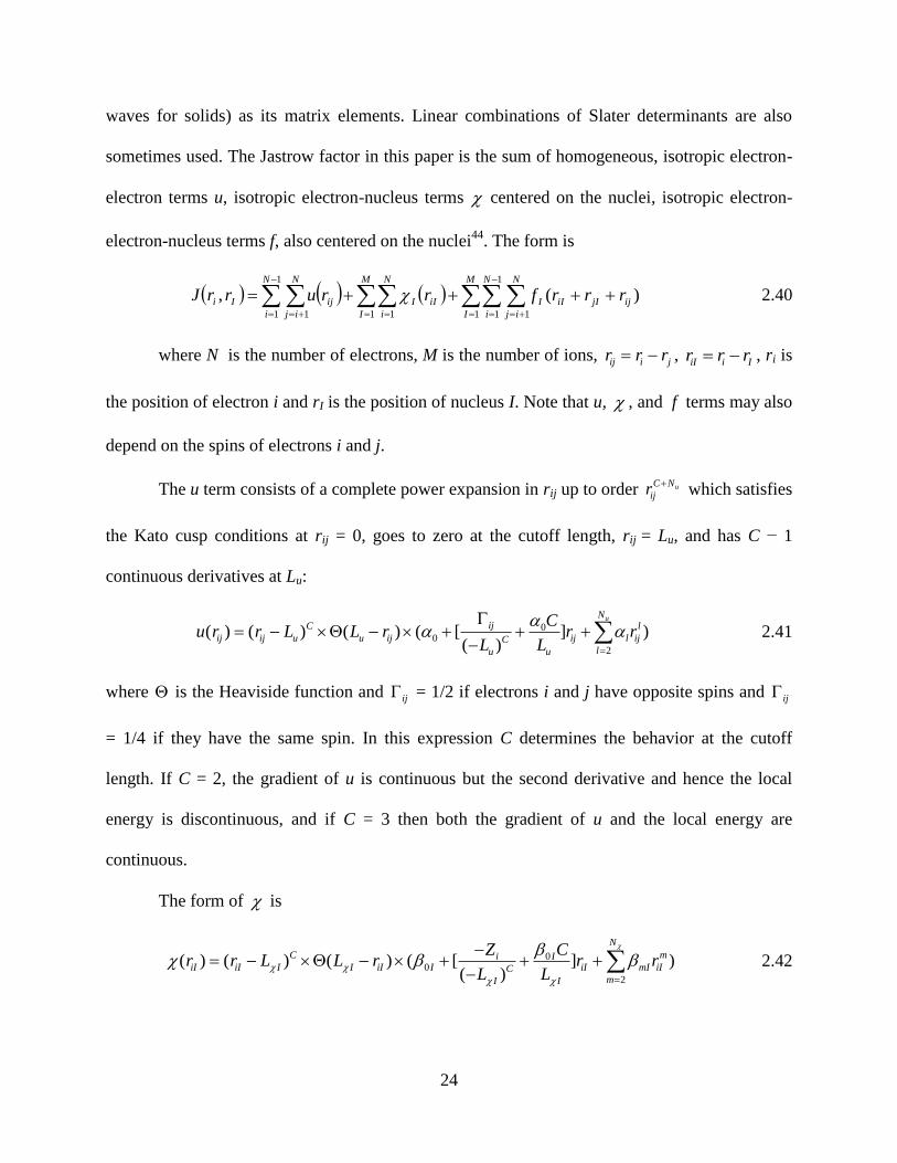
24
waves for solids) as its matrix elements. Linear combinations of Slater determinants are also
sometimes used. The Jastrow factor in this paper is the sum of homogeneous, isotropic electron-
electron terms u, isotropic electron-nucleus terms centered on the nuclei, isotropic electron-
electron-nucleus terms f, also centered on the nuclei44
. The form is
M
I
N
i
N
ij
ijjIiII
M
I
N
i
iII
N
i
N
ij
ijIi rrrfrrurrJ1
1
1 11 1
1
1 1
)(, 2.40
where N is the number of electrons, M is the number of ions, ij i jr r r , iI i Ir r r , ri is
the position of electron i and rI is the position of nucleus I. Note that u, , and f terms may also
depend on the spins of electrons i and j.
The u term consists of a complete power expansion in rij up to order uC N
ijr
which satisfies
the Kato cusp conditions at rij = 0, goes to zero at the cutoff length, rij = Lu, and has C − 1
continuous derivatives at Lu:
00
2
( ) ( ) ( ) ( [ ] )( )
uNijC l
ij ij u u ij ij l ijClu u
Cu r r L L r r r
L L
2.41
where is the Heaviside function and ij = 1/2 if electrons i and j have opposite spins and ij
= 1/4 if they have the same spin. In this expression C determines the behavior at the cutoff
length. If C = 2, the gradient of u is continuous but the second derivative and hence the local
energy is discontinuous, and if C = 3 then both the gradient of u and the local energy are
continuous.
The form of is
00
2
( ) ( ) ( ) ( [ ] )( )
N
C mi IiI iI I I iI I iI mI iIC
mI I
Z Cr r L L r r r
L L
2.42

25
It may be assumed that mI =
mJ where I and J are equivalent ions. The term involving
the ionic charge ZI enforces the electron-nucleus cusp condition.
The expression for f is the most general expansion of a function of rij , riI and rjI that does
not interfere with the Kato cusp conditions and goes smoothly to zero when either riI or rjI reach
cutoff lengths:
0 0 0
( , , ) ( ) ( ) ( ) ( )
eN eN eefI fI fIN N N
C C l m n
I iI jI ij iI fI jI fI fI iI fI jI lmnI iI jI ij
l m n
f r r r r L r L L r L r r r r
2.43
Various restrictions are placed on lmnI . To ensure the Jastrow factor is symmetric under
electron exchanges it is demanded that , , ,lmnI mlnIl I m l n . If ions I and J are equivalent then it
is demanded that lnlmnI m Jl .

26
3.0 THE QMC STUDY OF THE BE ATOM
3.1 INTRODUCTION
With the development of the ab initio methods, one can determine the electronic structure of
systems with many electrons only by invoking a number of approximations. For systems like
beryllium with only a few electrons, high-level "complete" nonrelativistic calculations are within
reach, and these benchmark calculations have become important sources of information
concerning the accuracy of the various algorithms, approximations, and basis sets.
The HF description of the ground state of the Be atom (1S) gives the electronic
configuration 1s22s
2. However, because the 1s
22p
2 electronic configuration is almost degenerate
with the previous one, Beryllium is also challenging for the ab initio techniques.
3.2 COMPUTATIONAL DETAILS
We did all-electron calculations of the ground-state energy of the Be atom using the variational
and diffusion quantum Monte Carlo (VMC and DMC) methods. Accurate approximations to the
many-electron wave function are required as inputs for the VMC and DMC methods45
. The
quality of these “trial” wave functions determines both the statistical efficiency of the methods
and the final accuracy that can be obtained.

27
Several different forms of trial wave function were used here: (a) RHF orbitals with
optimized Jastrow function, (b) UHF orbitals with optimized Jastrow function, (c) Brueckner
Doubles (BD)46,47
orbitals with optimized Jastrow function, and (d) CASSCF orbitals with
optimized Jastrow function.
The basic form of the wave functions consists of a product of Slater determinants for
spin-up and spin-down electrons containing the orbitals, such as RHF, UHF, and BD orbitals,
multiplied by a positive Jastrow correlation factor. We have also carried out some tests using
multideterminant wave functions like CASSCF orbitals in the study.
The RHF, UHF, BD, and CASSCF orbitals forming the Slater determinants were
obtained from the calculations using Gausian03 code48
. 6-311G(d) basis sets were used for all
calculation.
All the variational and diffusion quantum Monte Carlo (VMC and DMC) calculations
were performed using the CASINO code49
. In the VMC calculation, the number of equilibration
moves at the start of the calculation is all set to be 5000, which are substantially large enough in
order to ensure that all of the transient effects due to the initial distribution die away. The total
VMC steps are set to be 40000. All of the DMC calculations were performed with a target
population of 1200 configurations (walkers). The parameters in the Jastrow functions were
obtained by minimizing the variance of the local energy50,51
. All of the energies were
extrapolated to zero time step.

28
3.3 RESULTS
In Table 3.1 we present values for the total nonrelativistic energies of the Be atom, calculated
using a number of different electronic-structure methods. For comparison, We give results
obtained using RFH, UHF, BD, and Cas(2,4) methods with 6-311G(d) basis sets, as well as the
VMC and DMC methods with the RHF, UHF, BD, and Cas(2,4) trail wave functions,
respectively.
Table 3.1 Total energy of the Be atom calculated with different ab inito methods, and the experimental result.
Method Energy (a.u.)
RHF/6-311G(d) -14.5718739
UHF/6-311G(d) -14.5722037
BD/6-311G(d) -14.6172223
Cas(2,4)/6-311G(d) -14.6118491
HF52
-14.573023
VMC-RHF (no Jastrow function) -14.567(7)
VMC-UHF (no Jastrow function) -14.575(4)
VMC-BD (no Jastrow function) -14.575(4)
VMC-Cas(2.4) (no Jastrow function) -14.621(7)
VMC-RHF (with Jastrow function) -14.6296(7)
VMC-UHF (with Jastrow function) -14.6244(9)
VMC-BD (with Jastrow function) -14.6266(9)
VMC-Cas(2.4) (with Jastrow function) -14.660(1)
DMC-RHF -14.6577(7)
DMC-UHF -14.6560(5)
DMC-BD -14.6581(4)
DMC-CAS(2,4) -14.6663(3)

29
CCSD(T)/cc-pVTZ53
-14.623790
FCI/cc-pVTZ53
-14.623810
Explicitly correlated Gaussians54
-14.667355(1)
Experiment, minus relativistic corrections53
-14.66736(1)
Experiment52
-14.6693324(1)
We performed both VMC(no Jastrow function) and VMC (with Jastrow function)
calculations. The results of VMC-RHF(no Jastrow function), VMC-UHF(no Jastrow function),
and VMC-Cas(2,4) (no Jastrow function) agree with that of RHF, UHF, and Cas(2.3) method,
since the VMC energy is calculated as the expectation value of the Hamiltonian operator with
respect to a trial wave function. However, the result of VMC-BD(no Jastrow function) does not
match that of the BD method, but agrees with that of the HF method. It is not surprised because
in the absence of the perturbation, the single Brueckner determinant, which is used in the VMC
calculation, is identical with the Hartree-Fock single determinant47
. With the optimized Jastrow
function, all of the VMC results with different trial wave functions are improved. Our VMC
energeis with RHF+Jastrow, UHF+Jastrow, BD+Jastrow, and Cas(2,4)+Jastrow are -14.6296(7),
-14.6244(9), -14.6266(9), and -14.660(1), respectively. These values are lower than the energies
from CCSD(T)/cc-pVTZ and FCI/cc-pVTZ calculations. However, the accuracy of a VMC
simulation was entirely limited by the quality of the trial wave function. While they are lower
than their respective RHF, UHF, BD, and CASSCF equivalents, they are still significantly higher
than our DMC energies and the “exact” result.
In DMC calculations, all of the energies were extrapolated to zero time. We used a range
of small time steps and performed linear extrapolations of the energies to zero time step. The
DMC energies with all of the four different trial wave functions, RHF, UHF, BD, and Cas(2,4),
are at most 12 mhartree, above the exact result of -14.667355(1). The DMC energy with Cas(2,4)

30
nodal surface performs best, which is only about 1 mhartree above the exact one. Therefore, all
of the four trial wave functions, RHF, UHF, BD, and Cas(2,4), can provide agreeable nodal
surfaces for the fixed-node DMC calculation of the Be atom. The DMC-Cas(2,4) can give the
best result in all of the four choices of the trial wave functions.
Multi-determinant wave functions, such as Cas(2,4), performs better than single-
determinant wave functions. However, the DMC energy with Cas(2,4) and 6-311G(d) basis set is
still 1 mhartree higher than the exact one. To obtain more improvement, more active spaces
Cas(2, 10) in which 2s2p3s3d orbitals are included, are applied as trial functions in the DMC
calculations. Two different basis sets, CVB255
and ADF-QZ4Pae-f56
were used to compare to 6-
31G(d) basis set to see which one can provide a better nodal surface. Table 3.2 shows the DMC
energy of the Be atom with different Cas(2,4) and Cas(2,10) trial functions with different basis
sets. It can be seen that with the same active space Cas(2,4) including 2s2p, the DMC energy
with CVB1basis set is about 0.0009 hartree lower than the one with 6-31G(d) basis sets. With
Cas(2,10) (2s2p3s3d) trial functions, the DMC energy with CVB2 basis set performs better than
the one with ADF basis set for about 0.0004 hartree. The trial function Cas(2,10) with CVB2
basis set gives the best nodal surface and the DMC energy is very close to the exact result of -
14.667355(1), and only about 0.00006 hartree higher.
Table 3.2 DMC energy of the Be atom calculated with different Cas trial functions.
Method Energy (a.u.)
DMC-CAS(2,4)/6-31G(d) -14.6663(3)
DMC-CAS(2,4)/CVB1 -14.66727(1)57
DMC-CAS(2,10)/CVB2 -14.66729(3)
DMC-CAS(2,10)/ADF -14.66687(5)
Explicitly correlated Gaussians54
-14.667355(1)
31
4.0 THE QMC STUDY OF WATER DIMER
4.1 INTRODUCTION
Water is the main agent of all aqueous phenomena. It is also an important component of the vast
majority of all chemical and biological processes. The description of the structure and energetics
of assemblies of water molecules has been the subject of many experimental and theoretical
studies, as this knowledge is vital to the understanding of water in all its physical states.
The characteristic physical and chemical properties of water are mostly from its hydrogen
bonds. In spite of the apparent simplicity of hydrogen bonding, understanding hydrogen bonding
remains a challenge, due in part to the relative weakness of the interaction.
The water dimer has been the subject of many electronic structure studies58-61
, since it
represents the prototype of all hydrogen-bonded systems. Despite its apparent simplicity,
accurate theoretical descriptions of the water dimer have typically required the use of very large
basis sets in combination with sophisticated wave function techniques, such as the configuration
interaction (CI) method and the coupled cluster (CC) method. These methods can perform high
accuracy. However they are slowly convergent and scale badly with system size. They also
suffer from basis set superposition and basis set incompleteness errors. Density functional theory
(DFT) is a computationally economical choice. Unfortunately, DFT meet challenges to treat
dispersion interactions accurately, which is important for studying hydrogen bond systems.

32
The Quantum Monte Carlo (QMC) method is another promising choice in situations
where high accuracy is required. We performed all-electron variational quantum Monte Carlo
(VMC) and diffusion quantum Monte Carlo (DMC) calculations of the total energy of the water
monomer and dimer. The equilibrium dissociation energy De of the water dimer was deduced by
subtracting the sum of the energies of two monomers from the water dimer energy.
The accuracy of the VMC method depends crucially on the trial wave functions. The
fixed-node DMC energy also depends on the quality of the nodal surface of the trial wave
functions. Fortunately, the error induced by the fixed-node approximation should largely cancel
when energy differences, such as equilibrium dissociation energies, are calculated62
. This
cancellation was tested to be almost perfect for weakly bound systems63
. The trial wave function
of the Slater-Jastrow form, which consists of a product of Slater determinants and a positive
Jastrow function, was used in the VMC and DMC calculations. The Slater determinants were
obtained from Hartree-Fock (HF) method with aug-cc-pVDZ basis sets. The basis set used for
the DMC calculation can be smaller than that for other highly accurate methods, such as MP2, or
CCSD(T), since the energies obtained in the DMC method depend less strongly on the quality of
the basis set62
. The parameters in the Jastrow functions were obtained by minimizing the
variance of the local energy50,64
.
4.2 COMPUTATIONAL DETAILS
All the variational and diffusion quantum Monte Carlo (VMC and DMC) calculations were
performed using the CASINO code65
. In the VMC calculation, the number of equilibration
moves at the start of the calculation is all set to be 5000, which are substantially large enough in
33
order to ensure that all of the transient effects due to the initial distribution die away. The total
VMC steps are set to be 40000. All of the DMC calculations were performed with a target
population of 1600 configurations (walkers). Time-step errors have been carefully checked. All
of the energies were extrapolated to zero time step.
The calculations for the water monomer were carried out at the experimental equilibrium
geometry66
rOH=r’OH = 0.9572 Å and 104.52o
HOH .This geometry has been used in previous
calculations on the water monomer61,62,67
.
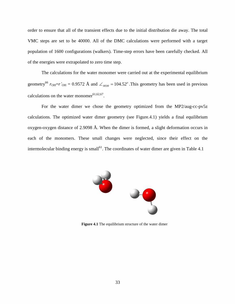
For the water dimer we chose the geometry optimized from the MP2/aug-cc-pv5z
calculations. The optimized water dimer geometry (see Figure.4.1) yields a final equilibrium
oxygen-oxygen distance of 2.9098 Å. When the dimer is formed, a slight deformation occurs in
each of the monomers. These small changes were neglected, since their effect on the
intermolecular binding energy is small61
. The coordinates of water dimer are given in Table 4.1
Figure 4.1 The equilibrium structure of the water dimer
34
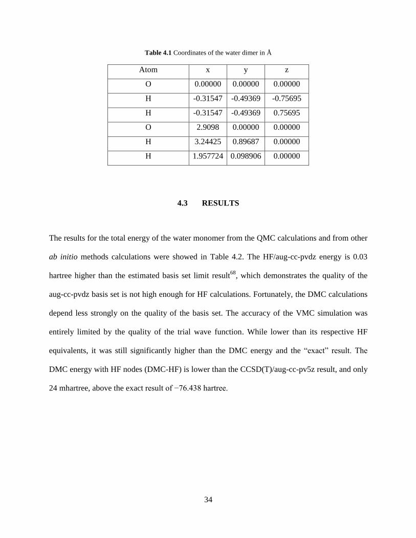
Table 4.1 Coordinates of the water dimer in Å
Atom x y z
O 0.00000 0.00000 0.00000
H -0.31547 -0.49369 -0.75695
H -0.31547 -0.49369 0.75695
O 2.9098 0.00000 0.00000
H 3.24425 0.89687 0.00000
H 1.957724 0.098906 0.00000
4.3 RESULTS
The results for the total energy of the water monomer from the QMC calculations and from other
ab initio methods calculations were showed in Table 4.2. The HF/aug-cc-pvdz energy is 0.03
hartree higher than the estimated basis set limit result68
, which demonstrates the quality of the
aug-cc-pvdz basis set is not high enough for HF calculations. Fortunately, the DMC calculations
depend less strongly on the quality of the basis set. The accuracy of the VMC simulation was
entirely limited by the quality of the trial wave function. While lower than its respective HF
equivalents, it was still significantly higher than the DMC energy and the “exact” result. The
DMC energy with HF nodes (DMC-HF) is lower than the CCSD(T)/aug-cc-pv5z result, and only
24 mhartree, above the exact result of −76.438 hartree.

35
Table 4.2 Total energies of the water monomer form various ab intio methods
Method Total energy (a.u.)
HF/aug -cc-pvdz -76.039
HF limit68 -76.068
CCSD(T)/aug-cc-pv5z69
-76.3703
VMC-HF -76.331(2)
DMC-HF -76.4141(5)
“Exact”70 -76.438
Table 4.3 Equilibrium dissociation energies of the water dimer from various ab initio methods and the experiment
Method De (kcal/mol)
DMC-HF (this work) -5.40±0.60
SAPT-5s71
-4.86
CCSD(T)-extrapolated72
-5.02±0.05
DMC (pseudopotential cal.)73
-5.66±0.20
DMC-HF62
-5.02±0.18
DMC-B3LYP62
-5.21±0.18
MP2/CBS limit74
-4.97
Table 4.3 shows the results for the equilibrium dissociation energy of the water dimer.
Our DMC energy with HF nodes (DMC-HF) compares very well within the error bars with the
CCSD(T) result of Klopper et al.72
and the MP2/CBS limit result of Xantheas et al.74
We obtain
a lower equilibrium dissociation energy of DMC-HF than that of Benedek et al.62
, although this
value is still within the error bars. It should be noted that Benedek et al. used the experimentally

36
determined equilibrium geometry, while we have used a theoretically optimized geometry. They
also performed larger DMC steps to obtain a smaller error bar.

37
5.0 THE QMC STUDY OF WATER CLUSTER ANION
5.1 INTRODUCTION
Water cluster anions provide a model system to unravel how hydrogen-bonded water network
deforms to accommodate the excess electron9 and help in understanding the free electron
hydration at a molecular level. Elucidation of the structures and formation mechanisms of
-
2(H O)n clusters is a challenging theoretical problem.75,76
In order to quantitatively characterize
such clusters using traditional electronic structure methods, it is necessary to employ flexible
basis sets with multiple diffuse functions and to include electron correlation effects to high order,
e.g. using the CCSD(T) method.76,77
Of particular interest are the vertical electron binding
energies (EBE), given by the differences in energies of the anionic and neutral clusters at the
geometries of the anions. EBEs of -
2(H O)n clusters up through n = 6 have been calculated using
the CCSD(T) method with large basis sets.78,79
In addition, EBEs of -
2(H O)n clusters as large as
-
2 30(H O) have been calculated using the MP2 method but with smaller basis sets.80-82
In some
geometrical arrangements there is the complication that the Hartree-Fock method provides a poor
description of the anion, and indeed, may even fail to bind the excess electron, which then poses
problems for perturbative methods such as MP2.81
In recent years a new generation of model potential approaches has been
developed for treating excess electrons interacting with water clusters.76,78,82
These model
38
potential approaches give EBEs close to the CCSD(T) results for the n ≤ 6 clusters for which
large basis set CSSD(T) calculations have been performed. It is also important to have accurate
ab initio results for large -
2(H O)n clusters that can serve as benchmarks for testing the
computationally faster model potential approaches. In this study, we use the diffusion Monte
Carlo (DMC) approach83-85
to calculate the electron-binding energies of two forms of -
2 6(H O) .
The DMC method is an intriguing alternative to traditional electronic structure approaches for
the characterization of -
2(H O)n clusters as its computational effort scales between the third and
fourth power with the number of molecules,86
and is applicable even in cases where the Hartree-
Fock approach does not provide a suitable zeroth-order wave function. The major challenge in
using the DMC method to calculate the electron binding energies of -
2(H O)n clusters is the need
to run the simulations on the neutral and anionic clusters for a sufficiently large number of
moves that the statistical errors in the EBEs are small compared to the EBE values themselves.
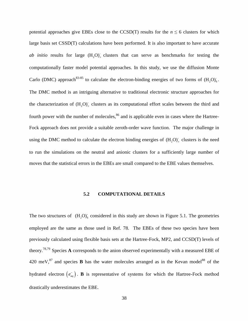
5.2 COMPUTATIONAL DETAILS
The two structures of -
2 6(H O) considered in this study are shown in Figure 5.1. The geometries
employed are the same as those used in Ref. 78. The EBEs of these two species have been
previously calculated using flexible basis sets at the Hartree-Fock, MP2, and CCSD(T) levels of
theory.78,79
Species A corresponds to the anion observed experimentally with a measured EBE of
420 meV,87
and species B has the water molecules arranged as in the Kevan model88
of the
hydrated electron aqe. B is representative of systems for which the Hartree-Fock method
drastically underestimates the EBE.

39
A
B
Figure 5.1 Geometrical structures of the A and B forms of (H2O)6-
The DMC calculations were carried out using single-determinental trial wave functions
obtained from Hartree-Fock or Becke3LYP89-92
density functional theory electronic structure
calculations, combined with three-term Jastrow factors93
to represent the electron-nuclear and

40
electron-electron cusps. The parameters in the Jastrow factors were obtained by minimizing the
local energy by means of variational Monte Carlo (VMC) calculations.94-96
A Hartree-Fock
pseudopotential97,98
was employed on the oxygen atoms in all calculations. The Hartree-Fock and
Becke3LYP calculations were carried out using the 6-31(3+)G contracted Gaussian-type basis
set of Ref. 81 on the H atoms and a 4s5p2d contracted Gaussian-type basis set on the O atoms.
The latter basis set was formed by adding two d functions, with exponents of 0.80 and 0.332, to
the Stuttgart ECP basis set for oxygen.99
For both isomers A and B, the Hartree-Fock method
underbinds the excess electron, while the Becke3LYP method overbinds it.
The wave functions and the configurations from the VMC calculations were used to carry
out the DMC calculations in the fixed-node approximation.86
Due to the diffuse nature of the
orbital occupied by the excess electron, errors caused by the fixed-node approximation are
expected to be nearly the same for the neutral and anionic clusters, and thus, should largely
cancel in the EBEs.37,100
The trial wave functions were generated using the Gaussian 03
program,101
and the VMC and DMC calculations were performed using the CASINO code.102
The DMC simulations were run using 4000 walkers, with 200000-300000 Monte Carlo steps per
walker, and for time steps of 0.003, 0.004, and 0.005 au. The results from the different time
steps were used to extrapolate the energies to 0 time step.85
5.3 RESULTS
The total energies of the neutral and anionic clusters of isomer A obtained using the various
methods are given in Table 5.1, and the corresponding results for isomer B are reported in Table
5.2. For isomer A, the DMC total energies obtained using the Hartree-Fock trial wave functions

41
are, within statistical errors, the same as those obtained using the Becke3LYP trial wave
functions, indicating that essentially the same nodal surfaces are obtained for the two types of
trial wave functions. For isomer B the DMC calculations using the Hartree-Fock trial wave
functions give somewhat higher (~0.014 au) total energies for both the neutral and anionic
clusters than do the DMC calculations using the Becke3LYP trial wave functions, indicating that
the B3LYP trial functions provide slightly better representations of the nodal surfaces in this
case.
Table 5.1 Total energies (au) of the neutral and anion of A
Methods Anion Neutral
HF -100.8067 -100.7961
B3LYP -102.7771 -102.7520
VMC-HF -102.805(5) -102.788(5)
VMC-B3LYP -102.569(7) -102.557(5)
DMC-HF -103.244(2) -103.226(2)
DMC-B3LYP -103.240(2) -103.224(2)
Table 5.2 Total energies (au) of the neutral and anion of B
Methods Anion Neutral
HF -100.7475 -100.7445
B3LYP -102.7184 -102.6789
VMC-HF -102.420(7) -102.404(7)
VMC-B3LYP -102.565(7) -102.555(7)
DMC-HF -103.175(3) -103.147(2)
DMC-B3LYP -103.189(2) -103.162(3)

42
The electron binding energies are summarized in Table 5.3. For isomer A the DMC
calculations with the HF and B3LYP trial wave functions give EBEs of 0.49±0.08 and 0.44±0.08
eV, respectively, in excellent agreement with the CCSD(T) result of 0.47 eV. For B the DMC
calculations with the HF and B3LYP trial wave functions give EBEs of 0.76±0.10 and 0.73±0.10
eV, respectively, again in excellent agreement with the CCSD(T) result of 0.78 eV. Most
strikingly, even though the Hartree-Fock method drastically underbinds the excess electron for
structure B, the DMC procedure is able to recover from this deficiency. For B the underbinding
of the excess electron in the Hartree-Fock approximation is greater in the present study than
found in Ref. 78. This is primarily a consequence of the neglect of p functions on the H atoms in
the basis set employed in the present study. To check whether this deficiency of the atomic basis
set impacts the EBE calculated with the DMC method, we have also carried out calculations for
structure B using a HF trial function generated using an expanded basis set formed by adding to
the basis set described above two p functions (from the aug-cc-pVDZ basis set103
) to each H
atom. This expanded basis set gives the same Hartree-Fock value of the EBE of B as reported in
Ref. 77. Moreover, the DMC/HF calculations with the expanded basis set give nearly the same
value of the EBE as of both the neutral and anionic species are lowered in energy by early the
same extent (~0.024 au) . Thus the DMC method is also very effective at overcoming limitations
in the atomic basis set. Most noteworthy is the finding that with the larger basis set, the statistical
errors in the total energies of B are considerly reduced, with the result that the statistical
uncertainty in the EBE is only 0.04 eV.
From Table 5.3 it is seen that for both structures A and B, the MP2 values of the EBEs
are, in fact, quite close to the CCSD(T) values. It should be noted, however, that there are other

43
arrangements of water molecules, for which the CCSD(T) values of the EBEs are much larger
than the MP2 values,104
and for which the DMC approach would be especially advantageous.
Table 5.3 Electron binding energies (EBE) (ev) of species A and B
Methods A B
HFa 0.29 (0.29) 0.08 (0.26)
B3LYP 0.68 1.07
MP2a 0.40 0.75
CCSD(T)a 0.47 0.78
VMC-HF 0.46±0.19 0.44±0.27
VMC-B3LYP 0.33±0.23 0.27±0.27
DMC-HF 0.49±0.08 0.76±0.10
DMC-B3LYP 0.44±0.08 0.73±0.10
a The MP2 and CCSD(T) EBEs of A and B are from Ref. 78. The Hartree-Fock results given in parenthesis
are also from Ref. 78
In this study we have shown that DMC calculations using either Hartree-Fock or
Becke3LYP trial wave functions give for the -
2 6(H O) cluster electron binding energies in
excellent agreement with the results of large basis set CCSD(T) calculations. Comparable
quality CCSD(T) calculations would be feasible for -
2 7(H O) and -
2 8(H O) but would be
computationally prohibitive on still larger water clusters. On the other hand, DMC calculations,
with their n3 scaling and high degree of parallelization, should be applicable to -
2(H O)n clusters
with n as large as 30. The finding that the diffusion Monte Carlo method gives nearly the same
EBEs with the Hartree-Fock and B3LYP trial wave functions is important as it means that one
can confidently employ B3LYP trial wave functions in cases where the Hartree-Fock procedure
fails to bind the excess electron.

44
6.0 THE QMC STUDY OF THE WATER-ACENE SYSTEMS
6.1 INTRODUCTION
The interactions between water and acene compounds are of fundamental importance in many
research areas. In material science and technology, this is partly associated with the practical
interest in carbon nanotubes (CNT), which have much promise in biosensor technology and other
applications involving water105,106
. A number of fundamental studies of the interactions water-
acenes systems also aimed at exploring the structural and phase behavior of water at the
nanometer scale5. Many properties of biological systems such as the structure of proteins, the
structure and function of biopolymers, and molecular recognition processes are influenced by the
interactions between acene molecules and water107
.
Water can interact with acene molecules in several ways. Both H atoms and the O
nonpaired electrons in H2O can participate in forming bonds between molecules. Most acene
compounds are immiscible in water, which indicates that the magnitudes of the interactions
between water and aromatic molecules are very weak.
Weak interactions possess a key role in physics and chemistry. Their respective strengths
determine the melting and boiling points as well as solvation energies and the conformation of
large biomolecules. The term “weak interactions” is the combined effect of electrostatic
repulsion or attraction, exchange repulsion, and dispersion attraction. Therefore a theoretical

45
treatment of the weak interactions requires an equally good and balanced description of each of
these effects.
Electrostatic interactions and exchange repulsion are in most cases sufficiently accurately
obtained with mean-field approaches such as Hartree-Fock (HF) and current implementations of
Kohn-Sham density-functional theory (DFT), but dispersion interactions on the other hand
originate from the correlated movement of electrons and are therefore not present in the HF
picture. DFT methods with a dispersion component seem to cover some dispersion interaction,
but unfortunately the performance is “far from generally applicable” and “having to be tailored
to the problem in question”19,108
The second-order Møller-Plesset perturbation (MP2) method and coupled cluster (CC)
method can perform high accuracy to study the dispersion interactions. However they are slowly
convergent and scale badly with system size. They also suffer from basis set superposition error,
basis set incompleteness error, and the linear dependency error when using large basis set for
large systems6. In a certain sense the QMC method appears like a natural choice for the
theoretical treatment of the weak interactions in water-acene systems.
6.2 THE QMC STUDY OF THE WATER-BENZENE COMPLEX WITH ALL-
ELECTRON TRIAL FUNCTIONS
6.2.1 Introduction
Benzene has the simplest structure of the acene family. An accurate treatment of this prototype
system is important for studying more complex water-acene systems. Many theoretical and

46
experimental investigations have been done for the benzene-water complex. Suzuki et al. first
indicated that benzene can form weak hydrogen bonds with water109
. The typical hydrogen bond
is stronger than the van der Waals bond but weaker than covalent or ionic bonds.
Experimentally, the rotationally resolved spectra of the benzene-water complex showed
that the water molecule is positioned above the benzene plane with both H atoms pointing
toward one face of the benzene, indistinguishably109,110
. Although the H positions were not
directly located in those experiments, they provided strong evidence for an interaction between
the proton donors (H atoms in water) and the proton acceptors (the benzene π cloud). From a
theoretical point of view, MP2 and CCSD(T) calculations show that, the most stable
configuration for the water-benzene system is that of water positioned above the center of the
benzene ring with a single H atom pointing toward the benzene and the other pointing away from
it111,112
. However, The energy difference between these two configurations is very small108,113
.
Figure 6.1 MP2-optimized global minimum structure of the water-benzene complex

47
6.2.2 Computational details
Figure 6.1 shows the geometry of the water-benzene complex which was used in our QMC
calculations. It is given by the MP2/6-31+G[2d,p] optimization, which is close to those obtained
from MP2 and CCSD(T) calculations with larger basis sets112
. The optimized geometry of the
benzene monomer agrees well with the experiment data: rCC =1.397 Å, and rCH =1.084 Å 114
. The
interaction of the water monomer with the benzene ring causes the two OH bond lengths to
become unequal. One of the OH bonds is 0.967Å, in which the H atom π-bonded to the benzene
ring. The other one is 0.964Å, which is about 0.003 Å shorter than the π-bonded one, and 0.007
Å longer than the experimental one, 0.957 Å66
. For the benzene-water complex, the predicted
distance between the water and benzene centers of mass is 3.210 Å, which is considerably
shorter than the experimental values ranging from 3.32 to 3.35 Å. However, it is very close to
Feller‟s MP2 result with larger basis set, 3.211Å. The distance from the center of the benzene
ring to the hydrogen atom involved in the hydrogen bond is 2.306 Å in our calculation. This
value is about 0.007 Å short than the distance at the MP2/aug-cc -pVTZ level reported by
Feller112
.
Table 6.1 Equilibrium Dissociation Energy of the water-benzene system from various ab initio methods
Method De (kcal/mol)
MP2/6-31+G[2d,p]111
-2.83
MP2/CBS112
-3.9±0.2
MP2/CBS115
-3.61
CCSD(T)/CBS115
-3.28
DMC/HF/6-311++G** -3.4±0.3

48
6.2.3 Results
Table 6.1 shows our result for the dissociation energy from DMC calculations with HF/6-
311++G**trial wave functions, which is -3.4±0.3 kcal/mol. Fredericks and Jordan reported that
the dissociation energy of the water-benzene complex was -2.83 kcal/mol from the MP2
calculations using the 6-31+G[2d,p] basis set111
. Feller proposed the MP2 complete basis set
(CBS) limit dissociation energy, EMP2(CBSlimit), as -3.9±0.2 kcal/mol from the average of the BSSE
corrected EMP2(CBSlimit), -3.7kcal/mol and the BSSE not corrected MP2/cc-pVQZ interaction
energy of 4.1 kcal/mol112
. Feller also reported that the MP2 calculations slightly overestimate the
attraction (0.2-0.3 kcal/mol) compared to the CCSD(T) calculations using the aug-cc-pVDZ and
aug-cc-pVTZ basis sets112
. Jurecka et al. also reported the EMP2(CBSlimit) and ECCSD(CBSlimit)
complete basis set (CBS) limit dissociation energies as -3.61kcal/mol and -3.28 kcal/mol,
respectively115
.
The change in vibrational zero point energy (ZPE) for the reaction C6H6-H2O→C6H6 +
H2O can be obtained from normal-mode analyses, and amounts to 1.0 kcal/mol112
. Adding this to
our DMC electronic dissociation energy, yields ΔE0(0 K) = -2.4±0.3 kcal/mol, in good
agreement with the experimental value of ΔE0(0 K) = -2.25±0.28 kcal/mol116
, and ΔE0(0 K) = -
2.44±0.09117
.
An analysis of the time-step dependence of the equilibrium dissociation energy of the
water-benzene system for the DMC/ HF-6-311++G** calculations was performed. The result is
shown in Figure. 6.2. The time step errors in the monomer (water or benzene) and the water-
benzene complex calculations cancel a lot at small time steps. However, energy extrapolations to

49
0 time step for the monomers and the dimer are necessary for obtaining accurate electronic
dissociation energy of the water-benzene system.
-5.9
-5.4
-4.9
-4.4
-3.9
-3.4
-2.9
-0.001 0.001 0.003 0.005 0.007
Dissocia
tion
Energy
(kcal/mo
l)
Time step (a.u.)
Figure 6.2 Time-step dependence of the equilibrium dissociation energy of the water-benzene system for
the DMC/ HF-6-311++G** calculations
6.3 THE QMC STUDY OF THE WATER-ANTHRACENE COMPLEX WITH
PSEUDOPOTENTIAL
6.3.1 Introduction
Different from the benzene–water complex, which is well studied both experimentally and
theoretically, seldom experimental or theoretical data exist on the water-anthracene complex.
From a theoretical point of view, the water-anthracene system is too complex for MP2 and
CCSD methods with large enough basis set to give an accurate dissociation energy.

50
We performed pseudopotential QMC calculations of the water-anthracene system using
Slater-Jastrow wave functions with Hartree-Fock orbitals. The use of pseudopotentials in QMC
may introduce an additional source of error, the localization approximation. However, there are
several advantages to use pseudopotentials in the QMC calculations. One of the advantages of
using pseudopotentials is that they avoid the short-range variations in the wave function near the
nuclei, and hence the energy fluctuations will be largely reduced. It was also suggested that the
core electrons are responsible for much of the time-step bias118
. The time-step bias remains small
up to much larger time steps in the pseudopotential calculations. Thus we can use a larger time
step region, in which the trend of the energy extrapolation is still nearly linear, in
pseudopotential calculations than that in all electron calculations. It was verified in our DMC
calculations of the water-anthracene system (See Figure. 6.3). The pseudopotentials we used are
from the CASINO pseudopotential library119,120
. These pseudopotentials have been found to
work very well in conjunction with QMC methods61,121
.
-102.44
-102.43
-102.42
-102.41
-102.4
-102.39
-0.001 0.001 0.003 0.005 0.007 0.009Tota
l en
ergy
(a
.u.)
DMC time step (a.u.)
Extrapolation of the total energy of water-
anthracene
to zero time step
Figure 6.3 DMC energy of the water-anthracene complex as a function of the time step

51
6.3.2 Computational details
Figure. 6.4 shows the geometry of the water-anthracene complex, which was used in our
calculation. It is given by the MP2/aug-cc-pvdz optimization. For the anthracene monomer, rCC
=1.452 Å, and rCH =1.046Å. For the water monomer, the experimental equilibrium geometry66
was used, rOH=r’OH = 0.9572 Å and 104.52o
HOH . For the water-anthracene complex, the
predicted distance between the water and anthracene centers of mass is 3.137 Å. The distance
from the center of the anthracene face to the hydrogen atom involved in the hydrogen bond is
2.370 Å.
Figure 6.4 MP2-optimized structure of the water-anthracene complex
Table 6.2 Equilibrium Dissociation Energy of the water-anthracene system
Method De (kcal/mol)
SAPT/aug-cc-pVTZ122
-2.9
LMP2/aug-cc-pVTZ(-f) (CP)123
-3.0
DMC/HF-Pseudopotential -4.3±1.8

52
6.3.3 Results
Table 6.2 shows the result of the dissociation energy of the water-anthracene complex from the
pseudopotential DMC calculations with HF trial wave functions. We obtain a lower equilibrium
dissociation energy of DMC/HF-Pseudopotential than that of SAPT and LMP2 methods with
aug-cc-pVTZ basis set, although this value is still within the error bars. It should be noted that
the dissociation energy of the water-benzene system of LMP2/aug-cc-pVTZ(-f) (CP) method
was reported as -2.64 kcal/mol, which is 0.36 kcal/mol higher than that of the water-anthracene
system of LMP2/aug-cc-pVTZ(-f) (CP) method123
. The same trend, that the dissociation energy
of the water-anthracene system was lower than that of water-benzene system, was also reported
by Feller and Jordan6. Since our DMC result for the water-benzene system quite agrees with the
CCSD/CBS calculation and the experimental value, we suggested that the dissociation energy of
the water-anthracene system should be around the region of -3.4~-4.3 kcal/mol.
6.4 THE QMC STUDY OF LARGE WATER-ACENE SYSTEMS USING
LOCALIZED ORBITALS
6.4.1 Introduction
The QMC methods can give accurate studies for the water-benzene and water-anthracene
systems. However, it is evident that “accuracy” is not the only one that we should seriously
consider for water-anthracene and even larger water-ancene systems. The factor of “efficiency”
becomes much more important for studying larger interacting systems. Although the QMC

53
methods is highly parallelizable, and adapted to a broad definition of parallel computers, it is still
necessary to achieve better time scales of the QMC methods for studying large water-acene
complexes.
In standard QMC, the orbitals are HF or DFT eigenfunctions extending over the entire
system. Let the number of electrons in the system be N. The computational cost C of a stand
QMC calculation is, C = AN3+BN
4, where the N
3 term comes from (i) evaluating all N single-
particle orbitals and their derivatives at the N new electron positions (using localized basis
functions such as Gaussians), to reach a given target variance σ2
scaling as O(N), (ii) evaluating
the Jastrow factor, and (iii) evaluating the interaction energy. The N4 contribution arises from the
N updates of the matrix of cofactors, each of which takes a time proportional to N2, to reach a
given target variance σ2 proportional to N. Because B is of the order of 10
-4, the N
3 term
dominates in practice23
.
The rate-determining step in most QMC calculations is the evaluation of the orbitals in
the Slater wave function. If each of the N orbitals at the N electron positions is expanded in O(N)
basis functions (e.g. plane waves) then the time taken to evaluate the Slater wave function scales
as O(N3). On the other hand, if a localized basis set such as a cubic spline representation is used
then the time taken to evaluate each orbital is independent of system size, and hence the time
taken to evaluate the wave function scales as O(N2)124
. Finally, if the orbitals themselves are
spatially localized and truncated then the number of nonzero orbitals to evaluate at each electron
position is independent of system size, and so the time taken to compute the wave function is
O(N)27
. Remembering the factor of N from a target error bar σ2, the computational cost for
„localized‟ QMC calculation scales as O(N2), which allowed QMC calculations to be performed
for larger systems.

54
0
1000
2000
3000
4000
5000
6000
7000
8000
9000
0 20 40 60 80 100 120 140 160 180
Number of Electrons
Av
e. C
om
pu
tati
ng
Tim
e P
er B
lock
(Sec)
GTO-based trial function Localized plane-wave orbitals with B-splines functions
C2H4
C6H6
C14H10
C24H12
Figure 6.5 Computational cost of the DMC calculations for acene molecules as a function of the system
size
6.4.2 Computational details and results
The QMC calculations with localized plane-wave orbitals represented as spline functions were
performed to study benzene, anthracene, and coronene. The dash line in Figure 6.5 shows the
results of the computational cost of the localized DMC calculations. The solid line is the results
of the standard DMC calculations with Gaussian type obitals for ethylene, benzene, anthracene,
and coronene. For the acene molecules larger than anthracene, the localized DMC calculations
won out in the competition. However, the localized orbital calculations do not offer a huge
advantage due to: (1) localizing only the σ orbitals, and keeping π orbitals delocalized, and (2)
the need to use larger localization radii for the larger acenes.

55
6.5 THE QMC STUDY OF THE WATER-BENZENE AND WATER-CORONENE
COMPLEX WITH PSEUDOPOTENTIAL
6.5.1 Introduction
The interaction of molecules with acenes has attracted considerable interest for a variety of
reasons, including the use of such systems as models for understanding molecular adsorption on
graphene and graphite and for testing theoretical approaches for describing weak interactions.
Of particular interest is the magnitude of the interaction of a water molecule with the graphene
surface. This question has been addressed in numerous theoretical studies, with most of these
concluding that the binding energy of a water molecule to a graphene sheet is about -3.1
kcal/mol.125-127
However, diffusion Monte Carlo (DMC)83-85,128
and random-phase
approximation (RPA)129-131
calculations give significantly smaller (in magnitude) binding
energies (-1.6 and -2.3, respectively).132
In those studies using extrapolation of the results of
calculations of water-acene systems to obtain the water-graphene limit, water-benzene and
water-coronene systems play an important role.125,127
Based on the highest level calculations
available for these systems, the binding energies of water-benzene and water-coronene are about
-3.2 and -3.05 to -3.35 kcal/mol, respectively.125,127,133
In the case of water-benzene, the
theoretical estimates are in excellent agreement with the values deduced from experiment, while
there is no experimental value for the binding energy for the water-coronene system.
In extending electronic structure calculations to the larger acenes needed to realistically
model water interacting with graphene, there are multiple challenges. Foremost among these is
the fact that dispersion interactions play a major role in the binding.127
As a result, traditional
generalized gradient or hybrid density functional (DFT) methods are not suitable. This problem

56
is partially overcome by the use of dispersion-corrected DFT approaches. However, several such
approaches were recently tested for water-coronene and none were found to give a quantitatively
accurate description of the interaction potential.127
The MP2 method134,135
does include
dispersion interactions, but can overestimate their importance. Although this problem can be
solved by use of the CCSD(T) method,136-138
this approach (as traditionally formulated) is
computationally prohibitive for large acenes. In addition to the challenges posed by dispersion
interactions, traditional quantum chemistry methods using Gaussian-type orbitals are plagued by
near-linear dependency and basis set superposition error (BSSE)6,139
problems when applied to
molecules interacting with large acenes. Two of the most promising methods for characterizing
the interaction of water and other molecules with large acenes are DFT-based symmetry-adapted
perturbation theory with density fitting (DF-DFT-SAPT)140-142
and the MP2-C method of
Hesselmann.143,144
There are two implementations of the former – the DF-DFT-SAPT approach
of Hesselmann and co-workers141
and the DF-SAPT (DFT) method of Szalewicz and co-
workers.140,142
These methods display O(N5) scaling, where N is the number of electrons, and are
computationally attractive compared to CCSD(T). However, these approaches still suffer from
near-linear dependency problems when flexible basis sets containing diffuse functions are
employed. Moreover, the MP2, MP2C, and other methods that involve perturbative corrections
to the Hartree-Fock wave function might not be appropriate for large acenes due to their small
HOMO/LUMO gaps.
An alternative approach for calculating interaction energies, which is free of the problems
described above, is the diffusion Monte Carlo (DMC) method.83-85,128
This method has already
been applied to several weakly interacting systems, including water clusters37,145,146
and the
water-benzene dimer.147
In the usual fixed-node implementation,83,84
DMC calculations make use

57
of trial function – generally a Slater determinant comprised of Hartree-Fock (HF) or DFT
orbitals multiplied by a Jastrow factor93
to describe the electron-electron, electron-nuclear, and
electron-electron-nuclear correlations. DMC calculations afford the advantages of being
relatively insensitive to the basis set used for the trial function and having a relatively low, O(N3)
scaling, albeit with a large prefactor. The large prefactor is "compensated" by the fact that the
DMC calculations are highly parallel.
In this section, we use the DMC method with HF trial wave functions to calculate the
interaction energies of the water-benzene and water-coronene complexes. Water-benzene is
included to establish an appropriate Gaussian basis set for describing the trial functions. Two
different procedures for calculating the interaction energy are examined. One uses as the
reference the DMC energies of the isolated monomers and the other a DMC calculation on the
dimer with the two monomers far apart.
6.5.2 Computational Details
The structures of the water-benzene and water-coronene complexes considered in this study are
shown in Figure 6.6. The geometries employed are the same as those used in Ref. 126. For both
benzene and coronene, the experimental C-C bond length (1.420 Å) and C-C-C angles (120) for
graphite are employed.148
The acene C-H bond lengths and C-C-H angles were taken to be 1.09
Å and 120, respectively. The experimental gas-phase geometry is employed for the water
monomer, i.e., the O-H bond lengths are 0.9572 Å and the H-O-H angle is 104.52°.149
The water
molecule was placed above and perpendicular to the middle of the central ring, with both OH
groups pointing towards the acene, and an oxygen-ring distance of 3.36 Å127
as shown in Figure.
1. This distance came from an optimization of the geometry of water-coronene using the DF-

58
DFT-SAPT method.127
The experimentally observed water-benzene complex has minimum
energy structure with a "tilted" water molecule with one OH group pointed toward the center of
the ring.150
However, the energy difference between the one H-down minimum and the two H-
down saddle point structure is less than 0.2 kcal/mol.131,151,152
water-benzene
water-coronene
Figure 6.6 Geometrical structures of the water-benzene and water-coronene

59
The DMC calculations were carried out using single-determinant trial wave functions
obtained from Hartree-Fock calculations, combined with a three-term Jastrow factor93
to describe
the electron-electron, electron-nuclear, and electron-electron-nuclear correlations. The
parameters in the Jastrow factor were obtained by minimizing the local energy by means of
variational Monte Carlo (VMC) calculations.96
A Dirac-Fock pseudopotentials97,98
were
employed on all atoms. The Hartree-Fock calculations were carried out using modified versions
of the contracted Gaussian-type basis sets of Burkatzki, Filippi, and Dolg.153
For water-benzene,
three different basis sets were considered, the smallest of which (A) is the VDZ basis set
Burkatzki et al. which employs a 2s1p basis set for the H atoms and a 2s2p1d basis set for the C
and O atoms. The intermediate basis set (B) employs a 3s2p basis set for the H atoms and a
3s3p2d basis set for the C and O atoms, and was formed by adding the diffuse "aug" functions of
the aug-cc-pVDZ basis set154,155
to A. The largest basis set (C) employs 3s3p, 3s3p2d, 4s4p3d,
and 4s4p3d2f sets for acene-H, water-H, C, and O atoms, respectively. Basis set C was formed
by adding to the ATZ basis set of Burkatzki et al. the diffuse functions from the aug-cc-pVTZ
basis set,154,155
and omitting the f functions on the C atoms and the d functions on the acene H
atoms. As discussed below, DMC calculations on water-benzene give, within statistical errors,
the same interaction energy whether using basis set A, B, or C to represent for the trial function.
Although the computational effort of each DMC move grows with the complexity of the basis
set, the number of steps needed to achieve a specified convergence generally decreases as the
basis set is made more flexible. Basis set B represents a reasonable compromise and was adopted
for generating the trial function for water-coronene. However, linear dependency problems were

60
encountered in the Hartree-Fock calculations on water-coronene with this basis set, and to solve
this problem the diffuse exponents were scaled by a factor of two.
The wave functions and the configurations from the VMC calculations were used to carry
out the DMC calculations in the fixed-node approximation.83,84,86
The errors introduced by the
fixed-node approximation should largely cancel when the binding energies are calculated.37
The
trial wave functions were generated using the Gaussian 03 program,101
and the VMC and DMC
calculations were performed using the CASINO code.102,128
As mentioned above, two strategies were employed to obtain the binding energy. In the
first strategy (S1), the binding energy is calculated from the difference of energy of the water-
acene complex and the sum of energies of isolated acene and water molecules. In the second
strategy (S2), the energy of the water-acene complex at large separation is used in place of the
sum of the energies of the monomers. In each case the energies of the individual species are
extrapolated to the zero time step limit, and these extrapolated results are used to calculate the
zero-time-step binding energies. Although the final interaction energies obtained by
extrapolation to zero-time steps should not depend on which strategy is used, we are interested in
determining whether the errors due to the use of finite time steps largely cancel in the S2
strategy, as this would allow for a reduction in the computational effort.
For the water-benzene complex time steps of 0.003, 0.005, and 0.007 au were used in the
DMC calculations of the dimer, the isolated benzene molecule, and the isolated water molecule.
For the water-coronene system the calculations were performed for time steps of 0.005, 0.007,
and 0.01 au. The DMC simulations were run using total target populations of 4000-16000
walkers and a minimum of 70,000 Monte Carlo steps.

61
For the purpose of comparison, we also calculated the binding energy of water-coronene
using the direct RPA method.156
Three sets of RPA calculations were performed: (1) one using
the HF approximation to describe the first-order electrostatics and exchange repulsion and using
HF orbital to evaluate the RPA correlation energies, (2) using PBE157
orbitals to evaluate the
first-order electrostatics and exchange repulsion plus the RPA correlation corrections and (3)
applying the single-excitation correction to the RPA/PBE results.158
This last method is referred
to as RPA-s/PBE. The RPA calculations were performed with the FHI AIMS code159
using the
tier 3 basis set.160
6.5.3 Results
(a) Water-benzene
As seen from Table 6.3 and Figure 6.7, the binding energy of the water-benzene complex,
when calculated using the S1 strategy, shows a strong (linear) dependence on the time step and,
although the binding energies for basis sets B and C are significantly different at each time step,
they extrapolate to similar values in the zero time step limit (-3.26 ±0.26 and -3.01 ±0.26
kcal/mol, respectively). The results with the smallest basis set A, are not reported in the Table,
but they extrapolate to a value of -3.2±0.3 kcal/mol, consistent with those obtained with DMC
calculations using trial wave functions described with the larger basis sets.

62
Table 6.3 Total energy and binding energy of the water-benzene complex
methodsa water-benzene
(3.36 Å)(au)
benzene (au) water (au) water-
benzene
(12 Å) (au)
binding energy
(kcal/mol)
HF-B-S1 -53.31147 -36.43203 -16.87832 ** -0.70
HF-B-S2 -53.31147 ** ** -53.31040 -0.69
HF-C-S1 -53.37245 -36.47133 -16.89949 ** -1.02
HF-C-S2 -53.37245 ** ** -53.37086 -1.00
DMC-B-S1 -54.7807(2) -37.5737(3) -17.2018(2) ** -3.26±0.26
DMC-B-S2 -54.7807(2) ** ** -54.7756(3) -3.20±0.21
DMC-C-S1 -54.8020(3) -37.5880(2) -17.2092(2) ** -3.01±0.26
DMC-C-S2 -54.8020(3) ** ** -54.7972(3) -3.01±0.27
DMCb -3.4±0.3
CCSD(T)/CBSc -3.28
CCSD(T)/CBSd -3.20
CCSD(T)-F12e -3.21
Experimentf
(ZPE Corrected)
-3.25±0.28
Experimentg
(ZPE Corrected)
-3.44±0.09
a B:basis set B; C: basis set C; S1: strategy 1; S2: strategy 2.
b MP2/6-31+G[2d,p] level optimized geometry with rigid monomer.
c From Ref. 161.
d From Ref. 132.
e From Ref. 160.
f From Ref. 163.
g From Ref. 149.

63
Figure 6.7 Binding energy of water-benzene from DMC calculations using strategies S1 and S2 and basis
sets B and C
The binding energies obtained using the S1 and S2 procedures and extrapolation to the
zero time step limit are essentially identical. In addition, with the S2 procedure most of the bias
due to the use of finite time steps is removed from the result that, within the statistical errors, the
same binding energy is obtained for each time step. This is most encouraging because it means
that one can obtain accurate interaction energies by using the S2 procedure only a single time
step. Moreover, a reasonably large value of the time step can be used reducing the
computational time needed to achieve the desired convergence. With this approach, the
computational effort can be reduced by about a factor of five compared to that required for the
S1 procedure.
Our DMC values of the binding energy of water-benzene are in excellent agreement with
that (-3.21 kcal/mol)161
obtained from CCSD(T)-F12 calculations using the same geometry and

64
with complete basis set limit (CBS) CCSD(T) values, -3.20 and -3.28 kcal/mol,133,162
obtained
for the structure with one OH down.133
We also carried out DMC calculations for the water-
benzene complex with the one OH group down structure using the MP2/6-31+G[2d,p] level
optimized geometry, obtaining a value of -3.4 ± 0.3 kcal/mol for the binding energy. The
vibrational zero-point energy correction to the dissociation energy of water-benzene has been
estimated to be about 1.0 kcal/ mol.133,163
Applying this correction to our DMC result for the
MP2 optimized geometry we obtain a D0 value of -2.4 ± 0.3 kcal/mol in excellent agreement
with the experimental value of -2.44 ± 0.09 and -2.25±0.28 kcal/mol.150,164
(b) Water-coronene
The results for the water-coronene dimer are summarized in Table 6.4 and Figure 6.8.
From comparison of Figures 6.7 and 6.8, it is seen that with the S1 procedure the time step errors
are much greater for water-coronene than for water-benzene. However, with the S2 procedure,
the water-coronene interaction energy is relatively insensitive to the time step. As for water-
benzene, the interaction energy of water-coronene obtained from the two approaches - S1 with
extrapolation to zero time step and S2 using individual time steps - agree to within the statistical
errors. We take the S2 result with -0.007 au time step, -3.20 + 0.28 kcal/mol, as our best
estimate of the interaction energy between water-coronene at the employed geometry. (We
choose this value rather than that obtained from the S1 procedure due to the smaller statistical
error.)

65
Table 6.4 Binding energy of the water-coronene complex
methoda water-coronene
(au)
coronene (au) water (au) water-coronene
(15 Å) (au)
Binding energy
(kcal/mol)
HF-S1 -155.80389 -138.92435 -16.87836 ** -0.74
HF-S2 -155.80389 ** ** -155.80275 -0.71
DMC-S1 -160.4144(7) -143.2075(7) -17.2020(1) ** -3.07±0.57
DMC-S2-T1 -160.4548(3) ** ** -160.4497(3) -3.20±0.28
DMC-S2-T2 -160.4438(4) ** ** -160.4386(4) -3.26±0.35
DF-DFT-SAPTb
-3.05
CCSD(T)/CBSc -3.35
a S1 involves separate calculations on the two monomers at different time steps and extrapolation to zero time step,
while S2 uses a calculation on the dimer with a 15 Å separation between the water O and the center of the ring. T1:
time step 0.007 au; T2: time step 0.005 au.
b From Ref. 126.
c From Ref. 124.
Figure 6.8 Binding energy of water-coronene from DMC calculations using S1 and S2 strategies

66
We are unaware of any experimental values of the binding energy for the water-coronene
dimer. Probably the most accurate prior theoretical estimates of this binding energy are -3.05
and -3.35 kcal/mol from DFT-SAPT127
and CCSD(T)/CBS125
calculations, respectively. Within
the statistical error, the present DMC estimate of binding energy of water-coronene is consistent
with these values. We note that direct RPA calculations using PBE orbitals give a binding
energy of -2.5 kcal/mol (Table 6.5) when using the same geometry as employed for the DMC
calculations. However, the RPA-s/PBE method which includes a correction for single
excitations158
gives a binding energy of -3.0 kcal/mol in close agreement with the DMC, DFT-
SAPT, and CCSD(T) results.
Table 6.5 Binding energies (kcal/mol) of water-benezene, water-coronene, and water-graphene
water-benzene water-coronene water-graphene
DMC -3.2±0.2a 3.2±0.3
a -2.1
b
CCSD(T) -3.2c -3.3
d -3.1
e
DFT-CC -3.2f -3.3
d -3.1
d
DFT-SAPT -3.2g -3.0
g -3.0
g, h
RPA/HF -2.4i -2.1
a
RPA/PBE -2.5i -2.5
a -2.3
b
RPA-s/PBE -2.9i -3.0
a -2.8
j
a Present study.
b From Ref. 131. DMC value including correction for going from a single k-point to a suitable grid
of k points.
c From CCSD(T)/CBS calculations of Ref. 132.
d From Ref. 124.
e From Ref. 125. CCSD(T) result estimated using the incremental method.
f From Ref. 150.
g From Ref .126.
h Estimated from DFT-SAPT results for a series of water-acene systems.
i From Ref. 160.

67
j Estimated as described in the text.
The present study and earlier studies127,152,161
indicate that the binding energies of water-
acene systems are relatively insensitive to the size of the acene. At first sight this is surprising as
one would expect the induction and dispersion contributions to the binding to grow with
increasing size of the acene. However, as was observed in Refs. 126 and 151, the electrostatics
contribution decreases in magnitude with increasing size of the acene, roughly compensating for
the increasing magnitude of the dispersion contribution.
6.5.4 Conclusions
In this study, we demonstrate that the DMC method using a Hartree-Fock trial function gives
binding energies for water benzene and water-coronene that are consistent with the best prior
estimates of these quantities from ab initio calculations. It is found that the error due to the use
of finite time steps can be mitigated by the use of a DMC calculation of the two monomers at
large separation for obtaining the sum of the energies of the two non-interacting monomers. In
light of this and the O(N3) scaling of DMC calculations, it would be possible to extend these
calculations to water interacting with much larger acenes, for which it would be difficult, if not
impossible, to obtain CCSD(T)/CBS results.
It was noted in the Introduction that a recent DMC calculation gave a value of -1.6
kcal/mol for the binding of a water molecule to the graphene surface.132
This value is about 1.4
kcal/mol smaller (in magnitude) than obtained in other recent theoretical studies of water-
graphene.125-127
The DMC calculations of Ref. 131 were carried out using periodic boundary
conditions, a single k point, and with a supercell containing 50 carbon atoms. Based on the

68
results of RPA calculations, the authors of Ref. 131 established that the error due to use of the Г
point only for k-point sampling is about 0.5 kcal/mol. Applying this correction to their DMC
result gave a binding energy of -2.1 kcal/mol, which is still appreciably smaller in magnitude
than other recent estimates of the binding energy of water-graphene. Possible remaining errors
include the interactions between water molecules in adjacent cells and the inadequacy of a single
determinant wave function for describing the nodal surfaces. Give the spacing between the
water molecules, the error in the binding energy due to water-water interactions should be less
than 0.2 kcal/mol. This suggests that the use of a single determinant trial function introduces an
error of about 0.9 kcal/mol in the DMC value of the interaction energy for water-graphene. Ref.
131 also reported a RPA/PBE result of -2.26 kcal/mol for the water-graphene binding energy.
However, we have found that the binding energy of water-coronene grows in magnitude from -
2.5 to -3.0 kcal/mol in going from the RPA/PBE to the RPA-s/PBE method. This leads us to
conclude that the RPA-s/PBE procedure would give a binding energy close to -2.8 kcal/mol for
water-graphene, only slightly smaller in magnitude than the binding energies reported in Refs.
124, 125, and 126.

69
7.0 NEW GAUSSIAN BASIS SETS FOR QUANTUM MONTE CARLO
CALCULATIONS
7.1 INTRODUCTION
Quantum Monte Carlo methods,83,84
because of their cubic scaling with the number of atoms,
hold considerable promise for providing accurate interaction energies of molecular clusters. Most
quantum Monte Carlo electronic structure calculations make use of the fixed-node
approximation29,84
to enforce fermionic behavior on the wave function. The fixed nodal surface
is enforced by a trial function, generally taken to be a single Slater determinant of Hartree-Fock
or DFT orbitals, multiplied by the Jastrow factors93
to describe electron-electron and electron-
nuclei cusps. The parameters in the Jastrow factors are optimized by the use of the variational
Monte Carlo (VMC) procedure. The VMC step is generally followed by diffusion Monte Carlo
(DMC) calculations, which is where most of the computational effort is spent. The orbitals in
the trial functions used in quantum Monte Carlo calculations are most frequently represented in
terms of plane-wave or Gaussian-type orbitals (GTOs). In the former case, use of
pseudopotentials is essential to avoid the prohibitively high plane-wave cutoffs that would be
required for all-electron calculations. Moreover, even when using GTO basis sets, it is
advantageous to use pseudopotentials in quantum Monte Carlo calculations as this greatly
reduces the computational effort to achieve small statistical errors.

70
In our applications of quantum Monte Carlo methods employing trial functions expressed
in terms of GTOs and employing pseudopotentials, we observed surprising large variances of the
VMC energies. In some cases the variances were as much as a factor of six larger than obtained
with high cut-off plane-wave basis sets.165,166
This naturally raises concern about the impact of
such trial functions on the interaction energies obtained from subsequent DMC calculations. This
concern has led us to design for O, C, and H correlation-consistent GTO basis sets for use with
the Casino Dirac-Fock pseudopotentials.97,98
In this work we present these new correlation
constant basis sets to evaluate their performance in VMC and DMC calculations. In addition, we
examine the performance of two methods that have been designed for dealing with the problems
associated with using non-local pseudopotentials in quantum Monte Carlo calculations.
7.2 VMC CALCULATIONS
To illustrate the nature of the large variance problem when using certain GTO basis
set/pseudopotential combinations, we summarize in Table 7.1 the energies and variances from
VMC calculations on the water molecule using the Casino Dirac-Fock pseudopotential on the H
and O atoms and with the molecular orbitals in the trial functions represented either by the pVDZ
GTO basis set of Burkatzki, Filippi, and Dolg (BFD)153
, augmented with diffuse of s, p, and d
functions from the aug-cc-pVDZ basis set,154,155
or by plane-wave basis sets with energy cutoffs
of 60, 120, and 160 a.u.. The geometry of the water monomer was taken from experiment,149
with OH distances of 0.9572Å and an HOH angle of 105.52º. In the calculations using the
GTOs, the trial wave function was taken from Hartree-Fock calculations, and in the calculations
with the plane-wave basis set, the orbitals for the trial function were taken from local density

71
approximation (LDA) density functional theory calculations, with the orbitals being converted to
BLIP-type spline functions.167
In separate calculations using the augmented BFD basis set, we
confirmed that the energy and variance from the VMC calculations are nearly the same whether
using trial functions expanded in terms of Hartree-Fock or LDA orbitals. In all calculations,
three-term Jastrow factors were employed, the parameters in which were optimized so as to
minimize the variance of the energy. The Hartree-Fock calculations were carried out using the
Gaussian 03 package,168
and the DFT plane-wave calculations were carried out using ABINIT.169
The quantum Monte Carlo calculations were carried out using the CASINO code.128
The
calculations with the augmented BFD GTO basis set give a variance of 1.25 a.u. compared with
variances of 1.63, 0.34, and 0.26 a.u. obtained using plane-wave basis sets with cutoffs of 60,
120, and 160 a.u., respectively.
Table 7.1 VMC energies and variances for the water monomer using the Casino Dirac-Fock pseudopotential on all
atomsa
Basis set VMC energy (a.u.) Variance of the VMC energy (a.u.)
Augmented BFD -17.161(3) 1.25
Plane-wave/BLIP (60 a.u.)b -17.159(5) 1.63
Plane-wave/BLIP (120 a.u.)b -17.191(2) 0.34
Plane-wave/BLIP (160 a.u.)b -17.194(2) 0.26
a. The molecular orbitals for the GTO and plane-wave basis sets were obtained from Hartree-Fock and LDA
calculations, respectively.
b. The plane-wave cutoff is given in parentheses.
Adding higher angular momentum functions to the augmented BFD GTO basis set had
little effect on the variance. This led us to examine the variances obtained in all-electron VMC
calculations using Dunning's cc-pVDZ, cc-pVTZ, cc-pVQZ, cc-pV5Z, and cc-pV6Z basis
sets,155
omitting g and higher angular momentum functions, as these are not supported by the

72
Casino code. The variances of the VMC energy for the above sequence of basis sets are 3.6, 2.4,
1.5, 1.1, and 0.8 a.u., respectively. Similar variances are obtained with the corresponding aug-cc-
pVXZ basis sets basis sets.154,155
Due to the large contribution of the 1s electrons to the total
energies, the variance in the complete basis set limit is necessarily larger in all-electron than in
pseudopotential calculations. These results suggested that the large variance found in the VMC
calculations with the extended augmented BFD basis set is due to the fact that this basis set is far
from optimal for use with Casino Dirac-Fock pseudopotential. Although high quality aug-cc-
pVXZ- type basis sets for use with pseudopotentials have been developed for heavier
elements,170-172
such basis sets have not been developed for Li-Ne, primarily due to the fact that
with traditional quantum chemistry methods, there is little computational advantage to replacing
the 1s orbitals by pseudopotentials. However, as noted above, the use of pseudopotentials to
model the 1s electrons of Li-Ne is more advantageous in quantum Monte Carlo calculations.
With this in mind, we have designed a series of correlation consistent basis sets for oxygen and
carbon with the core 1s electrons described by Casino Dirac-Fock pseudopotentials. In addition,
to facilitate comparison with calculations employing trial functions expressed in terms of plane-
wave basis sets, we also developed analogous basis sets for use with the Casino Dirac-Fock
pseudopotential for hydrogen. These basis sets are designated as aug-cc-pVDZ (CDF), aug-cc-
pVTZ (CDF), aug-cc-pVQZ (CDF), and aug-cc-pV5Z (CDF) and are described in Table 7.2-7.4.
Table 7.2 aug-cc-pVXZ basis sets for oxygen in Gaussian09 format
Aug-cc-pVDZ Aug-cc-pVTZ Aug-cc-pVQZ Aug-cc-pV5Z S 4 1.0
11.4406 0.08363
7.27416 -0.207273
0.95278 0.573366 0.29088
0.541479
S 6 1.0
10.1546 0.096389
6.37 -0.283037
3.98674 0.050966
1.79565 0.128286
S 8 1.0
18.84472 -0.029516
11.79099 0.182223
7.3841 -0.360446
4.6178 0.167268
S 10 1.0
58.03297 -0.002591
36.23793 0.01985
22.65517 -0.082116
14.16847 0.208792

73
S 1 1.0
0.29088 1.0
S 1 1.0
0.0888 1.0
P 4 1.0
7.5686 0.107913
2.4382 0.260983
0.86732 0.440022
0.26935 0.421942
P 1 1.0
0.26935 1.0
P 1 1.0
0.0727 1.0
D 1 1.0
1.21925 1.0
D 1 1.0
0.3269 1.0
0.72768 0.587155
0.25211 0.413898
S 1 1.0
1.79565 1.0
S 1 1.0
0.25211 1.0
S 1 1.0
0.0873 1.0
P 6 1.0
16.73989 -0.019406
10.48574 0.082373
4.00777 0.127921
1.74357 0.287838
0.64569 0.451838
0.20487 0.313232
P 1 1.0
0.64569 1.0
P 1 1.0
0.20487 1.0
P 1 1.0
0.0581 1.0
D 1 1.0
2.32444 1.0
D 1 1.0
0.65656 1.0
D 1 1.0
0.2053 1.0
F 1 1.0
1.42299 1.0
F 1 1.0
0.4847 1.0
2.88657 -0.193426
1.69534 0.312394
0.61236 0.592491
0.22118 0.324558
S 1 1.0
1.69534 1.00
S 1 1.0
0.61236 1.00
S 1 1.0
0.22118 1.00
S 1 1.0
0.0799 1.00
P 8 1.0
27.46118 0.002418
16.24763 -0.032846
10.16013 0.125286
6.35703 -0.073485
3.98208 0.20842
1.35787 0.374914
0.47123 0.432846
0.16354 0.210237
P 1 1.0
1.35787 1.00
P 1 1.0
0.47123 1.00
P 1 1.0 0.16354
1.00
P 1 1.0
0.0538 1.00
D 1 1.0
3.66083 1.00
D 1 1.0
1.27681 1.00
D 1 1.0
0.44532 1.00
8.7684 -0.245096
3.44237 -0.084054
2.30015 0.109763
0.96585 0.423202
0.40557 0.488075
0.1703 0.16071
S 1 1.0
2.30015 1.00
S 1 1.0
0.96585 1.00
S 1 1.0
0.40557 1.00
S 1 1.0
0.1703 1.00
S 1 1.0
0.0715 1.00
P 10 1.0
53.20848 -0.001496
33.08254 0.009418
20.59562 -0.035314
12.88695 0.06608
5.61128 0.086196
3.51864 0.016914
2.20676 0.245761
0.8669 0.386175
0.34056 0.340201
0.13378 0.136243
P 1 1.0
2.20676 1.00
P 1 1.0
0.8669 1.00
P 1 1.0
0.34056 1.00
P 1 1.0
0.13378 1.00

74
D 1 1.0
0.1469 1.00
F 1 1.0
2.61391 1.00
F 1 1.0
0.85131 1.00
F 1 1.0
0.3128 1.00
G 1 1.0
1.83814 1.00
G 1 1.0
0.6998 1.00
P 1 1.0
0.0471 1.00
D 1 1.0
5.31609 1.00
D 1 1.0
2.14461 1.00
D 1 1.0
0.86518 1.00
D 1 1.0
0.34903 1.00
D 1 1.0
0.1236 1.00
F 1 1.0
4.01865 1.00
F 1 1.0
1.56803 1.00
F 1 1.0
0.61183 1.00
F 1 1.0
0.2306 1.00
G 1 1.0
3.22935 1.00
G 1 1.0
1.18195 1.00
G 1 1.0 0.4938
1.00 H 1 1.0
2.29924 1.00
H 1 1.0
1.0069 1.00
Table 7.3 aug-cc-pVXZ basis sets for hydrogen in Gaussian09 format
Aug-cc-pVDZ Aug-cc-pVTZ Aug-cc-pVQZ Aug-cc-pV5Z S 4 1.0 13.01 0.018161
1.962 0.140114
0.4446 0.476695 0.122 0.501665
S 5 1.0 33.87 0.003021
5.095 0.048453
1.159 0.199653 0.3258 0.506418
S 6 1.0 82.64 -0.000376
12.41 0.016339
2.824 0.075323 0.7977 0.257107
S 8 1.0 402 0.000022
60.24 -0.000597
13.73 0.013185 3.905 0.043733

75
S 1 1.0
0.122 1.00 S 1 1.0
0.0297 1.00
P 1 1.0 0.7364 1.00
P 1 1.0
0.1419 1.00
0.1027 0.382386
S 1 1.0 0.3258 1.00
S 1 1.0
0.1027 1.00 S 1 1.0
0.0254 1.00
P 1 1.0 1.4452 1.00
P 1 1.0
0.3902 1.00 P 1 1.0
0.1009 1.00
D 1 1.0 1.0762 1.00
D 1 1.0
0.2499 1.00
0.2581 0.497216
0.08989 0.296149 S 1 1.0
0.7977 1.00
S 1 1.0 0.2581 1.00
S 1 1.0
0.08989 1.00 S 1 1.0
0.0236 1.00
P 1 1.0 2.7109 1.00
P 1 1.0
0.8905 1.00 P 1 1.0
0.2925 1.00
P 1 1.0 0.0833 1.00
D 1 1.0
1.9684 1.00
D 1 1.0
0.6364 1.00
D 1 1.0 0.1822 1.00
F 1 1.0
1.5518 1.00 F 1 1.0
0.3759 1.00
1.283 0.143398
0.4655 0.329949 0.1811 0.43703
0.07279 0.176123
S 1 1.0 1.283 1.00
S 1 1.0
0.4655 1.00 S 1 1.0
0.1811 1.00
S 1 1.0 0.07279 1.00
S 1 1.0
0.0207 1.00 P 1 1.0
4.6782 1.00
P 1 1.0 1.7361 1.00
P 1 1.0
0.6443 1.00
P 1 1.0
0.2391 1.00
P 1 1.0 0.0725 1.00
D 1 1.0
3.2691 1.00 D 1 1.0
1.2524 1.00
D 1 1.0 0.4798 1.00
D 1 1.0
0.1498 1.00 F 1 1.0
2.52 1.00
F 1 1.0 0.9124 1.00
F 1 1.0
0.2781 1.00 G 1 1.0
2.2151 1.00
G 1 1.0 0.5390 1.00
Table 7.4 aug-cc-pVXZ basis sets for carbon in Gaussian09 format
Aug-cc-pVDZ Aug-cc-pVTZ Aug-cc-pVQZ Aug-cc-pV5Z S 4 1.0
6.03476 0.081605 3.80212 -0.206235
0.48701 0.569109
0.15251 0.542776 S 1 1.0
0.15251 1.00
S 1 1.0 0.0478 1.00
P 4 1.0
3.55518 0.109803 1.16203 0.255434
0.42801 0.444751
0.1419 0.4064 P 1 1.0
0.1419 1.00
P 1 1.0 0.0407 1.00
D 1 1.0
0.5586 1.00 D 1 1.0
S 6 1.0
11.57792 -0.017912 7.2305 0.083429
3.57462 -0.208471
0.933 0.126287 0.37693 0.587742
0.1329 0.418306
S 1 1.0 0.933 1.00
S 1 1.0
0.1329 1.00 S 1 1.0
0.0469 1.00
P 6 1.0 7.89344 -0.019146
4.92416 0.08135
2.11811 0.093266 0.99366 0.25311
0.3817 0.451298
0.1284 0.360747 P 1 1.0
S 8 1.0
19.59101 0.007338 12.2387 -0.046054
7.18672 0.170523
4.49651 -0.238316 1.4262 -0.097824
0.8416 0.28021
0.3132 0.594111 0.1165 0.321281
S 1 1.0
0.8416 1.00 S 1 1.0
0.3132 1.00
S 1 1.0 0.1165 1.00
S 1 1.0
0.0434 1.00 P 8 1.0
14.28983 0.004438
8.93365 -0.031624 5.58553 0.079822
S 10 1.0
31.36778 -0.002416 19.53784 0.018709
12.19126 -0.078337
7.6152 0.201296 4.75817 -0.229367
1.92263 -0.088946
1.1955 0.094083 0.5105 0.403249
0.218 0.50158
0.0931 0.172148 S 1 1.0
1.1955 1.00
S 1 1.0 0.5105 1.00
S 1 1.0
0.218 1.00 S 1 1.0
0.0931 1.00
S 1 1.0 0.0397 1.00
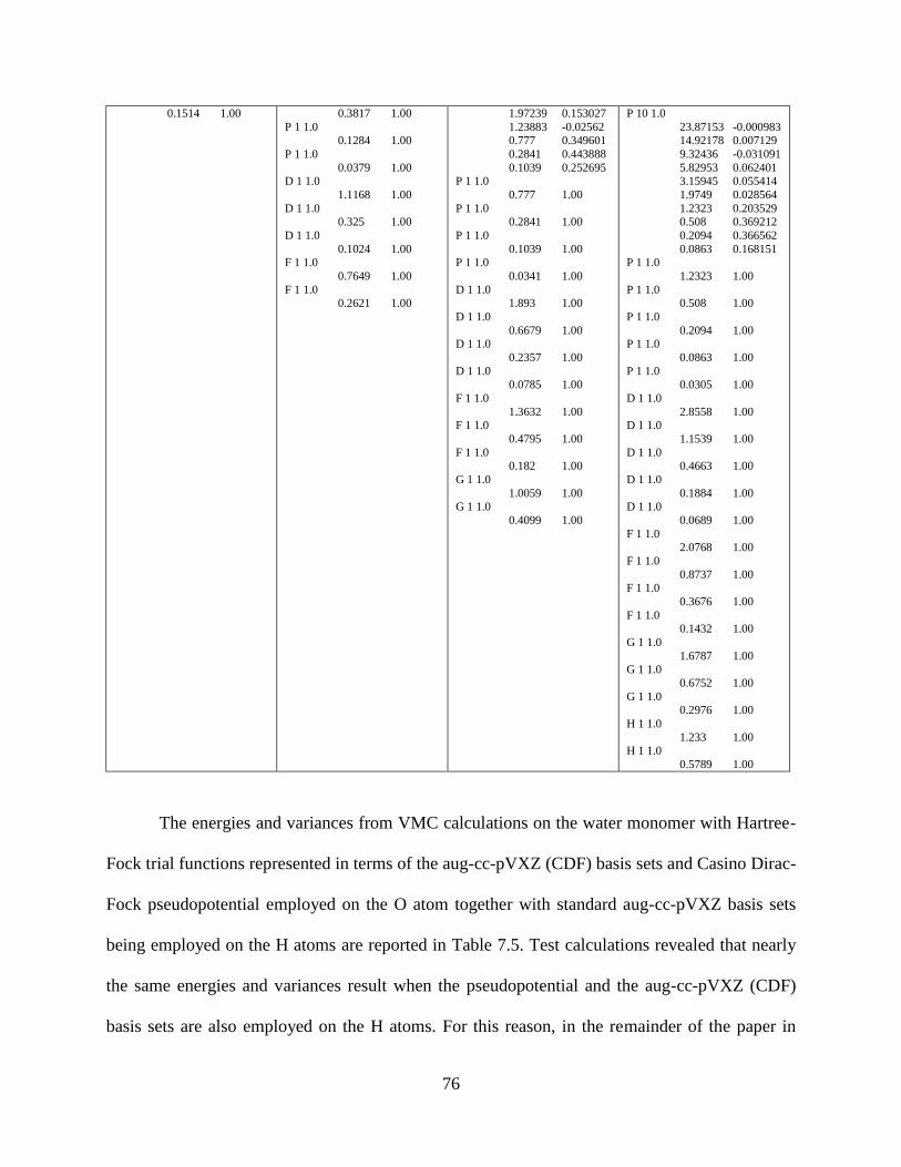
76
0.1514 1.00 0.3817 1.00
P 1 1.0 0.1284 1.00
P 1 1.0
0.0379 1.00 D 1 1.0
1.1168 1.00
D 1 1.0 0.325 1.00
D 1 1.0
0.1024 1.00 F 1 1.0
0.7649 1.00
F 1 1.0 0.2621 1.00
1.97239 0.153027
1.23883 -0.02562 0.777 0.349601
0.2841 0.443888
0.1039 0.252695 P 1 1.0
0.777 1.00
P 1 1.0 0.2841 1.00
P 1 1.0
0.1039 1.00 P 1 1.0
0.0341 1.00
D 1 1.0 1.893 1.00
D 1 1.0
0.6679 1.00 D 1 1.0
0.2357 1.00
D 1 1.0
0.0785 1.00
F 1 1.0
1.3632 1.00 F 1 1.0
0.4795 1.00
F 1 1.0 0.182 1.00
G 1 1.0
1.0059 1.00 G 1 1.0
0.4099 1.00
P 10 1.0
23.87153 -0.000983 14.92178 0.007129
9.32436 -0.031091
5.82953 0.062401 3.15945 0.055414
1.9749 0.028564
1.2323 0.203529 0.508 0.369212
0.2094 0.366562
0.0863 0.168151 P 1 1.0
1.2323 1.00
P 1 1.0 0.508 1.00
P 1 1.0
0.2094 1.00 P 1 1.0
0.0863 1.00
P 1 1.0
0.0305 1.00
D 1 1.0
2.8558 1.00 D 1 1.0
1.1539 1.00
D 1 1.0 0.4663 1.00
D 1 1.0
0.1884 1.00 D 1 1.0
0.0689 1.00
F 1 1.0 2.0768 1.00
F 1 1.0
0.8737 1.00 F 1 1.0
0.3676 1.00
F 1 1.0 0.1432 1.00
G 1 1.0
1.6787 1.00 G 1 1.0
0.6752 1.00
G 1 1.0 0.2976 1.00
H 1 1.0
1.233 1.00 H 1 1.0
0.5789 1.00
The energies and variances from VMC calculations on the water monomer with Hartree-
Fock trial functions represented in terms of the aug-cc-pVXZ (CDF) basis sets and Casino Dirac-
Fock pseudopotential employed on the O atom together with standard aug-cc-pVXZ basis sets
being employed on the H atoms are reported in Table 7.5. Test calculations revealed that nearly
the same energies and variances result when the pseudopotential and the aug-cc-pVXZ (CDF)
basis sets are also employed on the H atoms. For this reason, in the remainder of the paper in

77
presenting results using GTO basis sets for the trial functions, the Casino Dirac-Fock
pseudopotential and aug-cc-pVXZ (CDF) basis sets are used only for the O atoms. From Table
7.5, it is seen that with the aug-cc-pVDZ (CDF) basis set, the variance in the energy is reduced
about threefold and the VMC energy is about 0.03 a.u. lower compared to the corresponding
results obtained using the augmented BFD basis set on the O atom. With the aug-cc-pVTZ
(CDF) basis set, the variance further is reduced to 0.29 au, which is very close to the value
obtained with the plane-wave basis set with the 160 a.u. cutoff. For the largest GTO basis set
considered, aug-cc-pV5Z (CDF), the variance is 0.22 a.u. As for the all-electron calculations,
the results obtained with the larger GTO basis sets omitted the g and higher angular momentum
functions from the O basis set and the f and higher angular momentum functions from the H
basis set. However, given the fact that the energies and variances obtained with the aug-cc-pVTZ
(CDF), and modified aug-cc-pVQZ (CDF) and aug-cc-pV5Z (CDF) basis sets are very close to
those obtained with large cutoff plane-wave calculations, we conclude that the higher angular
momentum functions are relatively unimportant for VMC calculations.
Table 7.5 VMC energies and variances for the water monomera
Basis set VMC energy (a.u.) Variance of the VMC energy (a.u.)
Aug-cc-pVDZ (CDF) -17.193(2) 0.42
Aug-cc-pVTZ (CDF) -17.197(1) 0.29
Aug-cc-pVQZ (CDF) -17.199(1) 0.23
Aug-cc-pV5Z (CDF) -17.200(1) 0.22
a. Results obtained employing a pseudopotential on the O atom only, with the standard aug-cc-pVXZ basis
sets being used on the H atoms.

78
7.3 DMC CALCULATIONS
Figure 7.1 reports the results of DMC calculations on the water monomer with trial functions
expanded in terms of the augmented BFD, the aug-cc-pVDZ (CDF), and aug-cc-pVTZ (CDF)
GTO basis sets, as well as the 60 and 120 a.u. cutoff plane-wave basis sets. The DMC
simulations were run using 10,000 walkers, about 35,000 Monte Carlo steps, and for time steps
of 0.003, 0.005, 0.012, and 0.02 a.u., using the T-move procedure.173,174
Figure 7.1 DMC energy of the water molecule with different trial functions
In each case the energies for the various time steps are well represented by linear fits,
facilitating extrapolation to zero time step. Several trends are apparent from the data in this
figure. First, DMC calculations using trial functions with the largest variances, namely those

79
expanded in terms of the augmented BFD and 60 a.u. cutoff plane-wave basis sets, display the
large dependencies of the energies on the time step. Secondly, the DMC calculations with
different trial functions give different total energies in the t0 limit. The trial function using the
augmented BFD basis set gives the highest DMC energy, -17.20207(9) a.u., and that represented
in terms of plane-wave basis set with 120 a.u. cutoff, gives the lowest DMC energy, -17.2186(2).
The calculations using the aug-cc-pVDZ (CDF) and aug-cc-pVTZ (CDF) basis sets give
extrapolated DMC energies of -17.2117(1) and -17.21341(9), respectively. Of course, for typical
applications, the relevant question is how the various methods perform at calculating energy
differences. This will be examined below, where we report binding energies for the water dimer.
However, before examining the binding energies we first consider the sensitivity of the total
energies to the choice of the Jastrow factor and to the strategy, T-move173,174
or locality
approximation (LA),175
used to deal with errors introduced in the local approximation to the
pseudopotential. Two different choices of the Jastrow factors are used, one obtained from a
variance minimization and the other from an energy minimization.
In DMC calculations with pseudopotentials, the use of a non-local potential is
incompatible with the fixed-node boundary condition, and the two schemes mentioned above can
be used to deal with the problem. Each scheme has its advantages and disadvantages. The LA is
believed to have smaller time step bias, but to have more stability problems.176
In contrast, the T-
move procedure is believed to be more stable with an additional advantage of being variational,
but to require smaller time steps, especially for large systems.176,177
We also calculated the binding energy of water dimer to determine whether the fact that
different trial functions lead to different t0 extrapolated total energies impacts the energy
difference. Three different trial wave functions, HF with the aug-cc-pVTZ (CDF) basis sets, HF
80
with the augmented BFD basis set, and LDA with the plane-wave basis set (120 a.u. cutoff),
were used in the calculations. The geometries of the water monomer and dimer were optimized
at the MP2/aug-cc-pV5Z level. The optimized water dimer geometry has an equilibrium oxygen-
oxygen distance of 2.9098 Å. The binding energy for each method was calculated by subtracting
twice the energy of the monomer from the energy of the dimer.
Figure 7.2 reports the DMC total energies of water dimer obtained using different basis
sets and the two approaches for dealing with the nonlocal pseudopotential problem. In each
approach, two Jastrow factors were considered, one from variational minimization (Varmin) and
the other from energy minimization (Emin). As expected, the DMC calculations with the
augmented BFD basis set has the largest time step bias. Figure 7.3 shows on an expanded scale
the DMC results with the aug-cc-pVTZ (CDF) basis set. Most significantly, it is seen that in the
LA scheme the total DMC energy is more sensitive to the choice of Jastrow factor than when
using the T-move procedure. With the LA procedure when used with the aug-cc-pVTZ (CDF)
basis set, the two choices of Jastrow factors lead a difference of 0.5 kcal/mol in the total DMC
energies in the zero time step limit. The difference is even greater when using the trial function
represented in the plane-wave basis set. With the T-move scheme, the zero time step DMC
energies obtained using the two Jastrow factors agree to each other within the error bars, even
though the energy differences are significant at non-zero time steps. We were unable to perform
a stable DMC calculation with the LA approach using the trial function represented in terms of
the augmented BFD basis set, although such calculations ran smoothly with the aug-cc-pVTZ
(CDF) basis set which was optimized for use with the Casino pseudopotential.

81
Figure 7.2 DMC energies of the water dimer obtained using different basis sets for representing the orbitals,
different choices of Jastrow factors, and two strategies for dealing with the problems posed by
non-local pseudopotentials

82
Figure 7.3 Energies of the water dimer on an expanded scale, from DMC calculations using the
aug-cc-pVTZ (CDF) basis set
The DMC binding energies of water dimer obtained using HF orbitals expanded in terms
of the aug-cc-pVTZ (CDF) GTO basis set, the augmented BFD basis set, and LDA orbitals
expanded in terms of plane-wave basis set (120 a.u. cutoff) are reported in Table 7.6. The
binding energy is calculated from the difference of the DMC energies of the water dimer and
twice of the energies of the water monomer. As seen from Table 7.6, the DMC binding energies
from the various approaches agree to each other within the error bars. They also agree with the
DMC binding energies from prior all electron DMC calculations, as well as from complete-basis-
set limit CCSD(T) calculations.37,72
Interestingly, even though the trial functions employing
orbitals expanded in terms of the augmented BFD basis set have much larger variances in the
VMC step and larger time step biases in the DMC step, they give, to within the statistical errors,

83
binding energies in agreement with those from the other calculations. However, one has to be
cautious in generalizing this conclusion to more complex systems for which use of trial functions
with large variance may prove more problematical for energy differences. Aside from these
issues there is a decided efficiency advantage to using basis sets such as the aug-cc-pVXZ (CDF)
basis sets introduced here, which are optimized for using with pseudopotentials used in quantum
Monte Carlo calculations. For example, to achieve a specified statistical error in the DMC energy
of the water dimer about half the computer time is required for the aug-cc-pVTZ (CDF) basis set
than with the BFD basis set.
Table 7.6 Calculated binding energy of water dimer
Methods Binding Energy (kcal/mol)
DMC/avtz_T-move_Varmin -5.15±0.18
DMC/avtz_T-move_Emin -5.06±0.08
DMC/avtz_LA_Varmin -5.23±0.15
DMC/avtz_LA_Emin -5.21±0.15
DMC/BFD_T-move_Varmin -5.00±0.15
DMC/BFD_T-move_Emin -5.06±0.15
DMC/PL/BLIP_120_T-move_Varmin -5.15±0.18
DMC/PL/BLIP_120_T-move_Emin -5.16±0.09
DMC/PL/BLIP_120_LA_Varmin -5.16±0.18
DMC/PL/BLIP_120_LA_Emin -5.03±0.14
DMC/HF37
-5.02±0.18
DMC/B3LYP37
-5.21±0.18
CCSD(T) CBS limit72
-5.02±0.05
In this paper, we also tested two strategies to obtain the binding energy. In the first
strategy (S1) in Table 7.6, the binding energy is calculated from the difference of energy of the

84
water dimer and the sum of energies of two isolated water monomers. In the second strategy
(S2), the energy of the water dimer at large separation is used in place of the sum of the energies
of the two monomers. In the first case the energies of the individual species are extrapolated to
the zero time step limit, and these extrapolated results are used to calculate the zero-time-step
binding energies. In the second case, the zero-time-step binding energies were obtained by
extrapolating the binding energies with different time steps. Although the final interaction
energies obtained by extrapolation to zero-time steps should not depend on which strategy is
used, we are interested in determining whether the errors due to the use of finite time steps
largely cancel in the S2 strategy, as this would allow for a reduction in the computational effort.
Figure 7.4 Binding energies of water dimer with two different trial functions and strategies

85
As shown in Figure 7.4, the extrapolated zero-time-step binding energies obtained using
different trial functions and strategies are essentially identical. With the S1 procedure, there is
large time step bias for the binding energy with the BFD basis set plus Casino Dirac-Fock
pseudopotential, while most of the time step bias is cancelled when using CDF basis set plus
Casino Dirac-Fock pseudopotential. In addition, in the cases with the S2 procedure applying both
basis sets, most of the bias due to the use of finite time steps is removed form the result that,
within the statistical errors, the same binding energy is obtained for each time step. This is most
encouraging because it means that one can obtain accurate interaction energies by using the S2
procedure with only a single time step, no matter what the trial functions are applied. Moreover,
a reasonably large value of the time step can be used reducing the computational time needed to
achieve the desired convergence. With this approach, the computational effort can be reduced by
about a factor of five compared to that required for the S1 procedure with the BFD basis set plus
Casino Dirac-Fock pseudopotential.
7.4 CONCLUSIONS
In this work, we have developed for the C, O, and H atoms aug-cc-pVXZ (CDF) GOT basis sets
for use with the Dirac-Fock pseudopotentials from the Needs group. These basis sets give
greatly reduced variances compared to the GTO basis sets not designed for use with these
pseudopotentials. This, in turn, leads to significantly improved convergence behavior in
subsequent diffusion Monte Carlo calculations.

86
8.0 SUMMARY
In my dissertation research, I applied two particular variants of QMC, the variational Monte
Carlo (VMC) and diffusion Monte Carlo (DMC) methods, to study several interesting and
challenging electronic structure problems.
I carried out all-electron VMC and DMC calculations of the ground-state energy of the
beryllium atom with single-determinant and multi-determinant trial functions. Beryllium is also
challenging for the ab initio techniques because the near degeneracy of the 2s and 2p orbitals,
significantly distorts the symmetry of the Be atom, and makes the RHF wave function a
particularly poor choice. The resulting VMC energies with single-determinant trial functions
with optimized Jastrow factors only recover about 60% of the correlation energy, while the VMC
energy with a CASSCF trial function with optimized Jastrow factors recovers around 90% of the
correlation energy. The DMC energies with all trial wave functions are at most 12 mHartree
above the exact result of -14.667355(1) Hartree. The best DMC energy using a flexible CASSCF
trial function with the CVB2 basis set is only 0.00006 Hartree above the exact energy, which is
not only the best result in this study, but also the best DMC energy so far.
I performed all-electron VMC and DMC methods to calculate the total energy of the
water monomer and dimer, and used these to calculate the binding energy De of the dimer. For
the water monomer, the DMC total energy of water molecule with a HF trial function (DMC-HF)
is only 24 mHartree above the exact result of −76.438 Hartree. The DMC binding energy with a

87
HF trial function agrees, within the statistical error, with the CCSD(T) and the MP2/CBS limit
result.72,74
I also used the DMC method with Hartree-Fock and Becke3LYP trial functions to
calculate the electron binding energies of the -
2 6(H O) cluster, obtaining results in excellent
agreement with those of large basis set CCSD(T) calculations. Comparable quality CCSD(T)
calculations would be feasible for -
2 7(H O) and -
2 8(H O) but would be computationally prohibitive
for larger water clusters, due to its steep computational scaling. On the other hand, DMC
calculations, with their N3 (N is the number of electrons in the system) scaling and high degree of
parallelization, should be applicable to -
2(H O)n clusters with n as large as 30.
The VMC and DMC methods have also been applied in the all-electron calculations of
the binding energy of the water-benzene complex. The DMC dissociation energy matches very
well with the MP2(CBS-limit) and CCSD(T)(CBS-limit) results115
. Adding vibrational zero
point energy (ZPE) corrections to our DMC electronic binding energy gives ΔE0(0 K) = -2.4±0.3
kcal/mol, in good agreement with the experimental values of ΔE0(0 K) = -2.25±0.28 kcal/mol116
and ΔE0(0 K) = -2.44±0.09 kcal/mol.117
Pseudopotential QMC calculations have been performed to study the water-anthracene
complex using Slater-Jastrow wave functions with Hartree-Fock single-particle orbitals. The
resulting DMC binding energy agrees, within the error bars, with the results from Symmetry-
Adapted Perturbation Theory (SAPT) and local MP2 (LMP2) methods with the aug-cc-pVTZ
basis set.
It is also demonstrated that the DMC method using a Hartree-Fock trial function and the
Casino Dirac-Fock pseudopotential gives binding energies for water-benzene and water-
coronene that are consistent with the best prior estimates of these quantities from ab initio

88
calculations. It is found that the error due to the use of finite time steps can be mitigated by the
use of a DMC calculation of the two monomers at large separation for obtaining the sum of the
energies of the two non-interacting monomers. In light of this and the O(N3) scaling of DMC
calculations, it would be possible to extend these calculations to water interacting with much
larger acenes, such as hexabenzocoronene (C42H18) and circumcoronene (C54H18).
For large acene molecules, the DMC calculations with localized orbitals win out in the
competition of the computational cost. However, the localized orbital method in Casino does not
offer a huge advantage due to: (1) the current localization algorithm only localizing the σ orbitals
correctly, forcing us to keep the π orbitals delocalized, and (2) the need to use larger localization
radii for the larger acenes. In the future new algorithms to localize the π orbitals of π electron
systems should be developed, which would greatly improve the scaling of DMC calculations on
π electron systems.
Finally, newly designed correlation constant aug-cc-pVXZ (CDF) GTO basis sets have
been applied in the DMC calculations with the Dirac-Fock pseudopotentials from the Needs‟
group. These basis sets give greatly reduced variances compared to the GTO basis sets not
designed for use with these pseudopotentials. This, in turn, leads to significantly improved
convergence behavior in subsequent diffusion Monte Carlo calculations.
QMC methods, such as VMC and DMC method, represent a powerful tool for finding
solutions of the Schrödinger equation for atoms, molecules, and a variety of model systems.
They are among the most accurate many-body methods for extended systems. Their intrinsically
parallelizability makes them suitable for the current and next-generation massively parallel
computers.

89
QMC methods are not only suitable for computing the energy of the interacting systems
of electrons and fixed ions in the gas phase as described in this dissertation, but are also widely
used in the condensed systems. Applications of the DMC to the electronic structure of solids
include the properties of the homogeneous electron gas, cohesive energies of solids, equations of
state, phase transitions, lattice defects, surface phenomena, and excited states.178
Besides the VMC and DMC methods, other types of QMC methods are also increasingly
being used in different research areas. For example, auxiliary field Quantum Monte Carlo
(AFQMC) can be applied to treat excited states efficiently.179
Path integral Monte Carlo (PIMC)
is useful for high temperature electronic structure calculations and calculation of quantum
properties involving light ions.180
Coupled electron-ion Monte Carlo is good for low temperature
properties, where one needs to go beyond methods based on density functional theory,
particularly for disordered systems.180
Trial wave functions play an important role in the QMC methods as they determine the
accuracy of VMC results and provide the nodal surface for the DMC calculations. During recent
years, significant progress has been made in using more sophisticated trial wave functions and in
optimizing the parameters in them. Further advances are expected on this front.
In addition, force calculation in QMC methods is a topic of considerable research.181-184
For example, a stochastic line-minimization algorithm relying on Bayesian inference was
devised to find precise structural minima using energy estimates from accurate quantum Monte
Carlo calculations.185
Advances in this area will also stimulate progress in QMC-based
dynamical methods. Molecular dynamics methods compatible with VMC and PIMC have been
introduced by Miura.186
QMC/MD calculations with QMC forces have also been carried out of
liquid hydrogen to describe its properties under various thermodynamic conditions.187

90
REFERENCE
(1) Gervasio, F. L.; Chelli, R.; Procacci, P.; Schettino, V. Proteins 2002, 48, 117.
(2) Liu, H.; Elstner, M.; Kaxiras, E.; Frauenheim, T.; Hermans, J.; Yang, W. Proteins 2001,
44, 484.
(3) Appelbaum, I.; Wang, T.; Fan, S.; Joannopoulos, J. D.; Narayanamurti, V.
Nanotechnology 2001, 12, 391.
(4) Werder, T.; Walther, J. H.; Jaffe, R. L.; Halicioglu, T.; Koumoutsakos, P. J. Phys. Chem.
B 2003, 107, 1345.
(5) Sansom, M. S. P.; Biggin, P. C. Nature 2001, 414, 156.
(6) Feller, D.; Jordan, K. D. J. Phys. Chem. A 2000, 104, 9971.
(7) Gogotsi, Y.; Libera, J. A.; Gu vencü-Yazicioglu, A.; Megaridis, C. M. Appl. Phys. Lett.
2001, 79, 1021.
(8) Bahr, J. L.; Mickelson, E. T.; Bronikowski, M. J.; Smalley, R. E.; Tour, J. M. Chem.
Commun. 2001, 2, 193.
(9) Jordan, K. D.; Johnson, M. A. Science, 329, 42.
(10) Diedrich, C.; Luchow, A.; Grimme, S. J. Chem. Phys. 2005, 123, 184106.
(11) Tuckerman, M.; Laasonen, K.; Sprik, M.; Parinello, M. J. Chem. Phys. 1995, 103, 150.
(12) Pati, R.; Zhang, Y.; Nayak, S. K.; Ajayan, P. M. App. Phys. Lett. 2002, 81, 2638.
(13) Zhao, J.; Buldum, A.; Han, J.; Lu, J. P. Nanotechnology 2002, 13, 195.
(14) Parr, R. G.; Yang, W. Density-Functional Theory of Atoms and Molecules; Oxford
University Press: Oxford, 1989.
(15) Allen, M.; Tozer, D. J. J Chem Phys 2002, 117, 11113.
(16) Hobza, P.; Sponer, J.; Reschel, T. J. Comput Chem 1995, 11, 1315.

91
(17) Kristyan, S.; Pulay, P. Chem Phys Lett 1994, 229, 175.
(18) Elstner, M.; Hobza, P.; Frauenheim, T.; Suhai, S.; Kaxiras, E. J Chem Phys 2001, 114,
5149.
(19) Zimmerli, U.; Parrinello, M.; Koumoutsakos, P. J Chem Phys 2004, 120, 2693.
(20) Grimme, S. J Comput Chem 2004, 25, 1463.
(21) Friesner, R. Annu. Rev. Phys. Chem. 1991, 42, 34147.
(22) Collins, P. G.; Bradley, K.; Ishigami, M.; Zettl, A. Science 2000, 287, 1801.
(23) Foulkes, W. M. C.; Mitas, L.; Needs, R. J.; Rajagopal, G. Rev. Mod. Phys. 2001, 73, 33.
(24) R.J. Needs; M.D. Towler; etc. 2007.
(25) Towler, M. Phys. Stat. Sol. (b) 2006, 243, 2573.
(26) Williamson, A. J.; Hood, R. Q.; Grossman, J. C. Phys. Rev. Lett. 2001, 87, 246406.
(27) Alfè, D.; Gillan, M. J. J. Phys.: Condens. Mater. 2004, 16, 305.
(28) McMillan, W. L. Phys. Rev. 1965, 138 A442.
(29) Anderson, J. B. J. Chem. Phys. 1975, 63, 1499.
(30) Anderson, J. B. J. Chem. Phys. 1976, 65, 4121.
(31) Grimm, R. C.; Storer, R. G. J. Comput. Phys. 1971, 7, 134.
(32) Senatore, G., and N. H. March, . Rev. Mod. Phys. 1994, 66, 445.
(33) Ceperley, D. M. Rev. Mod. Phys. 1995a, 67, 279.
(34) Metropolis, N.; Rosenbluth, A. W.; Rosenbluth, M. N.; Teller, A. H.; Teller, E. J. Chem.
Phys. 1953, 21, 1087.
(35) Feller, W. An Introduction to Probability Theory and its Applications; Wiley, New York,
1968; Vol. 1.
(36) Hammond, B. L.; etc. Monte Carlo methods in Ab Initio quantum chemistry; World
Scientific Publishing Co. Pte. Ltd., 1994.
(37) Benedek, N. A.; Snook, I. K.; Towler, M. D.; Needs, R. J. J. Chem. Phys. 2006, 125,
104302.
(38) Reynolds, P. J.; Ceperley, D. M.; Alder, B. J.; and W. A. Lester, J. J. Chem. Phys. 1982,
77, 5593.

92
(39) Arnow, D. M.; Kalos, M. H.; Lee, M. A.; Schmidt, K. E. J. Chem. Phys. 1982, 77, 5562.
(40) Ceperley, D. M.; Alder, B. J. J. Chem. Phys. 1984, 81, 5833.
(41) Ceperley, D. M. J. Stat. Phys. 1991, 63, 1237.
(42) Kato, T. Communications on Pure and Applied Mathematics 1957, 10, 151.
(43) Jastrow, R. J. Phys. Rev. 1955, 98, 1479.
(44) Drummond, N. D.; Towler, M. D.; Needs, R. J. Phys. Rev. B 2004, 70, 235119.
(45) W. M. C. Foulkes; L. Mitas; R. J. Needs; G. Rajagopal. Rev. Mod. Phys. 2001, 73, 33.
(46) C. E. Dykstra. Chem. Phys. Lett. 1977, 45, 466.
(47) Handy, N. C.; Pople, J. A.; Head-Gordon, M.; Raghavachari, K.; Trucks, G. W. chemical
physics letters 1989, 164, 185.
(48) M. J. Frisch; G. W. Trucks; H. B. Schlegel; G. E. Scuseria; M. A. Robb; J. R.
Cheeseman; J. A. Montgomery; Jr., T. V.; K. N. Kudin; J. C. Burant; J. M. Millam; S. S.
Iyengar; J. Tomasi; V. Barone; B. Mennucci; M. Cossi; G. Scalmani; N. Rega; G. A.
Petersson; H. Nakatsuji; M. Hada; M. Ehara; K. Toyota; R. Fukuda; J. Hasegawa; M.
Ishida; T. Nakajima; Y. Honda; O. Kitao; H. Nakai; M. Klene; X. Li; J. E. Knox; H. P.
Hratchian; J. B. Cross; V. Bakken; C. Adamo; J. Jaramillo; R. Gomperts; R. E.
Stratmann; O. Yazyev; A. J. Austin; R. Cammi; C. Pomelli; J. W. Ochterski; P. Y. Ayala;
K. Morokuma; G. A. Voth; P. Salvador; J. J. Dannenberg; V. G. Zakrzewski; S.
Dapprich; A. D. Daniels; M. C. Strain; O. Farkas; D. K. Malick; A. D. Rabuck; K.
Raghavachari; J. B. Foresman; J. V. Ortiz; Q. Cui; A. G. Baboul; S. Clifford; J.
Cioslowski; B. B. Stefanov; G. Liu; A. Liashenko; P. Piskorz; I. Komaromi; R. L.
Martin; D. J. Fox; T. Keith; M. A. Al-Laham; C. Y. Peng; A. Nanayakkara; M.
Challacombe; P. M. W. Gill; B. Johnson; W. Chen; M. W. Wong; C. Gonzalez; J. A.
Pople. Gaussian 03; Revision C.02 ed.; Gaussian, Inc.: Wallingford CT, 2004.
(49) R. J. Needs; M. D. Towler; N. D. Drummond; P. López-Ríos. CASINO version 2.1.0
User Manual; University of Cambridge: Cambridge, 2007.
(50) Drummond, N. D.; R. J. Needs. Phys. Rev. B 2005, 72, 085124.
(51) P. R. C. Kent; R. J. Needs; G. Rajagopal. Phys. Rev. B 1999, 59, 12344.
(52) Martensson-Pendrill, A.; Alexander, S.; Adamowicz, L.; Oliphant, N.; Olsen, J.; Oster,
P.; Quiney, H.; Salomonson, S.; Sundholm, D. Phys. Rev. A 1991, 43, 3355.
(53) HARKLESS, J. A. W.; IRIKURA, K. K. International Journal of Quantum Chemistry
2006, 106, 2373.
(54) Komasa, J.; Rychlewski, J.; Jankowski, K. Phys Rev A 2002, 65, 042507.

93
(55) Ema, I.; Garcia De La Vega, J. M.; Ramirez, G.; Lopez, R.; Fernandez Rico, J.; Meissner,
H.; Paldus, J. J Comput Chem 2003, 24, 859.
(56) Van Lenthe, E.; Baerends, E. J. J. Comput. Chem. 2003, 24, 1142.
(57) Toulouse, J.; Umrigar, C. J. THE JOURNAL OF CHEMICAL PHYSICS 2008, 128,
174101.
(58) Park, C.-Y.; Kim, Y. J. Chem. Phys. 2001, 115, 2926.
(59) Feller, D. J. Chem. Phys 1992, 96, 6104.
(60) Tschumper, G. S.; Leininger, M. L.; Hoffman, B. C.; Valeev, E. F.; III, H. F. S.; Quack,
M. J. Chem. Phys. 2002, 116, 690
(61) Gurtubay, I. G.; Needs, R. J. J. Chem. Phys. 2007, 127, 124306.
(62) Benedek, N. A.; Snooka, I. K.; Towler, M. D.; Needs, R. J. J. Chem. Phys. 2006, 125,
104302.
(63) Mella, M.; Anderson, J. B. J. Chem. Phys. 2003, 119, 8225.
(64) Kent, P. R. C.; Needs, R. J.; Rajagopal, G. Phys. Rev. B 1999, 59, 12344.
(65) Needs, R. J.; Towler, M. D.; Drummond, N. D.; López-Ríos, P. CASINO version 2.1.0
User Manual; University of Cambridge: Cambridge, 2007.
(66) Benedict, W. S.; Gailar, N.; Plyler, E. K. J. Chem. Phys. 1956, 24, 1139.
(67) Lüchow, A.; Anderson, J.; Feller, D. J. Chem. Phys., 106, 77061997.
(68) Ermler, W.; Kern, C. J. Chem. Phys. 1974, 61, 3860.
(69) Halkier, A.; Koch, H.; Jorgensen, P.; Christiansen, O.; Nielsen, I. M. B.; Helgaker, T.
Theor. Chem. Acc. 1997, 97, 150.
(70) Feller, D.; Boyle, C.; Davidson, E. J. Chem. Phys. 1987, 86, 3424.
(71) Mas, E. M.; Bukowski, R.; Szalewicz, K.; Groenenboom, G. C.; Wormer, P. E. S.;
Avoird, A. v. d. J. Chem. Phys. 2000, 113, 6687.
(72) Klopper, W.; Rijdt, J. G. C. M. v. D.-v. d.; Duijneveldt, F. B. v. Phys. Chem. Chem. Phys.
2000, 2, 2227.
(73) Diedrich, C.; Lüchow, A.; Grimme, a. S. J. Chem. Phys. 2005, 123, 184106.
(74) Xantheas, S. S.; Burnham, C. J.; Harrison, R. J. J. Chem. Phys. 2002, 116, 1493.
(75) Lee, H. M.; Suh, S. B.; Kim, K. S. J. Chem. Phys. 2003, 118, 9981.

94
(76) Wang, F.; Jordan, K. D. Annu. Rev. Phys. Chem. 2003, 54, 367.
(77) Pople, J. A.; Head-Gordon, M.; Raghavachari, K. J. Chem. Phys. 1987, 10, 5968.
(78) Sommerfeld, T.; DeFusco, A.; Jordan, K. D. J. Phys. Chem. A 2008, 112, 11021.
(79) Gutowski, M. uppublished results.
(80) Herbert, J. M.; Head-Gordon, M. J. Phys. Chem. A 2005, 109, 5217.
(81) Herbert, J. M.; Head-Gordon, M. Phys. Chem. Chem. Phys. 2006, 8, 68.
(82) Williams, C. F.; Herbert, J. M. J. Phys. Chem. A 2008, 112, 6171.
(83) Anderson, J. B. J. Chem. Phys. 1975, 63, 1499.
(84) Anderson, J. B. J. Chem. Phys. 1976, 65, 4121.
(85) Foulkes, W. M. C.; Mitas, L.; Needs, R. J.; Rajagopal, G. Rev. Mod. Phys. 2001, 73, 33.
(86) Towler, M. D. Phys. Status Solidi B 2006, 243, 2573.
(87) Hammer, N. I.; Shin, J. W.; Headrick, J. M.; Diken, E. G.; Roscioli, J. R.; Weddle, G. H.;
Johnson, M. A. Science 2004, 306, 675.
(88) Feng, D.-F.; Kevan, L. Chem. Rev. 1980, 80, 1.
(89) Becke, A. D. Phys. Rev. A 1988, 38, 3098.
(90) Becke, A. D. J. Chem. Phys. 1993, 98, 5648.
(91) Lee, C.; Yang, W.; Parr, R. G. Phys. Rev. B 1988, 37, 785.
(92) Stephens, P. J.; Devlin, F. J.; Chabalowski, C. F.; Frisch, M. J. J. Phys. Chem. 1994, 98,
11623.
(93) Drummond, N. D.; Towler, M. D.; Needs, R. J. Phys. Rev. B 2004, 70, 235119.
(94) McMillan, W. L. Phys. Rev. 1965, 138, 442.
(95) Drummond, N. D.; Needs, R. J. Phys. Rev. B 2005, 72, 085124.
(96) Umrigar, C. J.; Toulouse, J.; Filippi, C.; Sorella, S.; Hennig, R. G. Phys. Rev. Lett. 2007,
98, 110201.
(97) Trail, J. R.; Needs, R. J. J. Chem. Phys. 2005, 122, 014112.
(98) Trail, J. R.; Needs, R. J. J. Chem. Phys. 2005, 122, 174109.

95
(99) Bergner, A.; Dolg, M.; Kuechle, W.; Stoll, H.; Preuss, H. Mol. Phys. 1993, 80, 1431.
(100) Mella, M.; Anderson, J. B. J. Chem. Phys. 2003, 119, 8225.
(101) Frisch, M. J.; Trucks, G. W.; Schlegel, H. B.; Scuseria, G. E.; Robb, M. A.; Cheeseman,
J. R.; Montgomery, J., J. A.; Vreven, T.; Kudin, K. N.; Burant, J. C.; Millam, J. M.;
Iyengar, S. S.; Tomasi, J.; Barone, V.; Mennucci, B.; Cossi, M.; Scalmani, G.; Rega, N.;
Petersson, G. A.; Nakatsuji, H.; Hada, M.; Ehara, M.; Toyota, K.; Fukuda, R.; Hasegawa,
J.; Ishida, M.; Nakajima, T.; Honda, Y.; Kitao, O.; Nakai, H.; Klene, M.; Li, X.; Knox, J.
E.; Hratchian, H. P.; Cross, J. B.; Bakken, V.; Adamo, C.; Jaramillo, J.; Gomperts, R.;
Stratmann, R. E.; Yazyev, O.; Austin, A. J.; Cammi, R.; Pomelli, C.; Ochterski, J. W.;
Ayala, P. Y.; Morokuma, K.; Voth, G. A.; Salvador, P.; Dannenberg, J. J.; Zakrzewski,
V. G.; Dapprich, S.; Daniels, A. D.; Strain, M. C.; Farkas, O.; Malick, D. K.; Rabuck, A.
D.; Raghavachari, K. F., J. B.; Ortiz, J. V.; Cui, Q.; Baboul, A. G.; Clifford, S.;
Cioslowski, J.; Stefanov, B. B.; Liu, G.; Liashenko, A.; Piskorz, P.; Komaromi, I.;
Martin, R. L.; Fox, D. J.; Keith, T.; Al-Laham, M. A.; Peng, C. Y.; Nanayakkara, A.;
Challacombe, M.; Gill, P. M. W.; Johnson, B.; Chen, W.; Wong, M. W.; Gonzalez, C.;
and Pople, J. A.; . Gaussian03; Gaussian, Inc. : Wallingford CT 2004.
(102) Needs, R. J.; Towler, M. D.; Drummond, N. D.; Ríos, P. L. CASINO version 2.3 User
Manual; University of Cambridge: Cambridge, 2008.
(103) Dunning, T. H. J. Journal of Chemical Physics 1989, 90, 1007.
(104) Xu, J.; Sommerfeld, T.; Jordan, K. D. Unpublished results.
(105) Erlanger, B. F.; Chen, B.-X.; Zhu, M.; Brus, L. Nano Lett. 2001, 1, 465.
(106) Huang, W.; Taylor, S.; Fu, K.; Lin, Y.; Zhang, D.; Hanks, T. W.; Rao, A. M.; Sun, Y.-P.
Nano Lett. 2002, 2, 311.
(107) Hunter, C. A. J. Mol. Biol. 1993, 230, 1025.
(108) Li, S.; Cooper, V. R.; Thonhauser, T.; Puzder, A.; Langreth, D. C. J.Phys. Chem. A 2008,
112, 9031.
(109) Suzuki, S.; Green, P. G.; Bumgarner, R. E.; Dasgupta, S.; Goddard, W. A., III; Blake, G.
A. Science 1992, 257, 942.
(110) Gutowsky, H. S.; Emilsson, T.; Arunan, E. J. Chem. Phys. 1993, 99, 4883.
(111) Fredericks, S. Y.; Jordan, K. D. J. Phys. Chem. A 1996, 100, 7810.
(112) Feller, D. J. Phys. Chem. A 1999, 103, 7558.
(113) Tsuzuki, S.; Honda, K.; Uchimaru, T.; Mikami, M.; Tanabe, K. J. Am. Chem. Soc. 2000,
122, 11450.

96
(114) Stoicheff, B. P. Can. J. Phys., 1954, 339.
(115) Jurecka, P.; Sponer, J.; Cerny, J.; Hobza, P. Phys. Chem. Chem. Phys. 2006, 8, 1985.
(116) Cheng, B.; Grover, J. R.; Walters, E. A. Chem. Phys. Lett. 1995, 232, 364.
(117) Courty, A.; Mons, M.; Dimicoli, I.; Piuzzi, F.; Gaigeot, M.; Brenner, V.; Pujo, P.; Millie,
P. J. Phys. Chem. A 1998, 102, 6590.
(118) Drummond, N. D.; Rıos, P. L.; Ma, A.; Trail, J. R.; Spink, G.; Towler, M. D.; Needs, R.
J. J. Chem. Phys. 2006, 124, 224104.
(119) Trail, J. R.; Needs, R. J. J. Chem. Phys. 2005, 122, 014112.
(120) Trail, J. R.; Needs, R. J. J. Chem. Phys. 2005, 122, 174109.
(121) Gurtubay, I. G.; Drummond, N. D.; M. D. Towler; Needs, R. J. J. Chem. Phys. 2006, 124,
024318
(122) Jenness, G. R.; Jordan, K. unpublished 2007.
(123) Reyes, A.; Fomina, L.; Rumsh, L.; Fomine, S. International Journal of Quantum
Chemistry 2005, 104, 335.
(124) Hernandez, E.; Gillan, M. J.; Goringe, C. M. PHYSICAL REVIEW B 1997, 55, 13485.
(125) Kysilka, J.; Rubes, M.; Grajciar, L.; Nachtigall, P.; Bludsky, O. J. Phys. Chem. A 2011,
115, 11387.
(126) Voloshina, E.; Usvyat, D.; Schutz, M.; Dedkov, Y.; Paulus, B. Phys. Chem. Chem. Phys.
2011, 13, 12041.
(127) Jenness, G. R.; Karalti, O.; Jordan, K. D. Phys. Chem. Chem. Phys. 2010, 12, 6375.
(128) Needs, R. J.; Towler, M. D.; Drummond, N. D.; Rıos, P. L. J. Phys.: Condens. Matter
2010, 22 023201.
(129) Nozieres, P.; Pines, D. Phys. Rev. 1958, 111, 442.
(130) Harl, J.; Kresse, G. Phys. Rev. Lett. 2009, 103, 056401.
(131) Lebegue, S.; Harl, J.; Gould, T.; Angyan, J. G.; Kresse, G.; Dobson, J. F. Phys. Rev. Lett.
2010, 105, 196401.
(132) Ma, J.; Michaelides, A.; Alfè, D.; Schimka, L.; Kresse, G.; Wang, E. Phys. Rev. B 2011,
84, 033402.
(133) Min, S. Y.; Lee, E. C.; Kim, D. Y.; Kim, D.; Kim, K. S. J. Comput. Chem. 2008, 29,
1208.

97
(134) Head-Gordon, M.; Pople, J. A.; Frisch, M. J. Chem. Phys. Lett. 1988, 153, 503.
(135) Møller, C.; Plesset, M. S. Phys. Rev. 1934, 46, 618.
(136) Deegan, M. J. O.; Knowles, P. J. Chem. Phys. Lett. 1994, 227, 321.
(137) Hampel, C.; Peterson, K. A.; Werner, H.-J. Chem. Phys. Lett. 1992, 190, 1.
(138) Raghavachari, K.; Trucks, G. W.; Pople, J. A.; Head-Gordon, M. Chem. Phys. Lett. 1989,
157, 479.
(139) Boys, S. F.; Bernardi, F. Mol. Phys. 1970, 19, 553.
(140) Misquitta, A. J.; Podeszwa, R.; Jeziorski, B.; Szalewicz, K. J. Chem. Phys. 2005, 123,
214103.
(141) Hesselmann, A.; Jansen, G.; Schutz, M. J. Chem. Phys. 2005, 122, 014103.
(142) Jeziorski, B.; Moszynski, R.; Szalewicz, K. Chem. Rev. 1994, 94, 1887.
(143) Pitonak, M.; Hesselmann, A. J. Chem. Theory Comput. 2009, 6, 168.
(144) Hesselmann, A. J. Chem. Phys. 2008, 128, 144112.
(145) Xu, J.; Jordan, K. D. J. Phys. Chem. A 2009, 114, 1364.
(146) Gurtubay, I. G. J. Chem. Phys. 2007, 127, 124306.
(147) Ma, J.; Alfe, D.; Michaelides, A.; Wang, E. J. Chem. Phys 2009, 130, 154303.
(148) King, H. W. CRC Handbook of Chemistry and Physics, 2007.
(149) Benedict, W. S.; Gailar, N.; Plyler, E. K. J. Chem. Phys. 1956, 24, 1139.
(150) Courty, A.; Mons, M.; Dimicoli, I.; Piuzzi, F.; Gaigent, M.-P.; Breener, V.; Pujo, P. d.;
Millie, P. J. Phys. Chem. A 1998, 102, 6590.
(151) Rubes, M.; Nachtigall, P.; Vondrasek, J.; Bludsky, O. J. Phys. Chem. C 2009, 113, 8412.
(152) Jenness, G. R.; Jordan, K. D. J. Phys. Chem. C 2009, 113, 10242.
(153) Burkatzki, M.; Filippi, C.; Dolg, M. J. Chem. Phys. 2007, 126, 234105.
(154) Kendall, R. A.; Dunning, T. H., Jr. ; Harrison, R. J. J. Chem. Phys. 1992, 96, 6796.
(155) Dunning, T. H., Jr. J. Chem. Phys. 1989, 90, 1007.
(156) Janesko, B. G.; Henderson, T. M.; Scuseria, G. E. J. Chem. Phys. 2009, 130, 081105.

98
(157) Perdew, J. P.; Burke, K.; Ernzerhof, M. Phys. Rev. Lett. 1996, 77, 3865.
(158) Ren, X.; Tkatchenko, A.; Rinke, P.; Scheffler, M. Phys. Rev. Lett. 2011, 106, 153003.
(159) Blum, V.; Gehrke, R.; Hanke, F.; Havu, P.; Havu, V.; Ren, X.; Reuter, K.; Scheffler, M.
Comput. Phys. Commun. 2009, 180, 2175.
(160) Havu, V.; Blum, V.; Havu, P.; Scheffler, M. J. Comput. Phys. 2009, 228, 8367.
(161) Jenness, G. R.; Karalti, O.; Al-Saidi, W. A.; Jordan, K. D. J. Phys. Chem. A 2011, 115,
5955.
(162) Jurecka, P.; Sponer, J.; Cerny, J.; Hobza, P. Phys. Chem. Chem. Phys. 2006, 8, 1985.
(163) Feller, D. J. Phys. Chem. A 1999, 103, 7558.
(164) Cheng, B. M.; Grover, J. R.; Walters, E. A. Chem. Phys. Lett. 1995, 232.
(165) Xu, J.; Jordan, K. D. J. Phys. Chem. A 2010, 114, 1364.
(166) Xu;, J.; Al-Saidi;, W. A.; Jordan, K. D. to be published.
(167) Alfè, D.; Gillan, M. J. Phys Rev B 2004, 70, 161101.
(168) Frisch, M. J.; Trucks, G. W.; Schlegel, H. B.; Scuseria, G. E.; Robb, M. A.; Cheeseman,
J. R.; Montgomery, J. A.; Jr., T. V.; Kudin, K. N.; Burant, J. C.; Millam, J. M.; Iyengar,
S. S.; Tomasi, J.; Barone, V.; Mennucci, B.; Cossi, M.; Scalmani, G.; Rega, N.;
Petersson, G. A.; Nakatsuji, H.; Hada, M.; Ehara, M.; Toyota, K.; Fukuda, R.; Hasegawa,
J.; Ishida, M.; Nakajim, T.; Honda, Y.; Kitao, O.; Nakai, H.; Klene, M.; Li, X.; Knox, J.
E.; Hratchian, H. P.; Cross, J. B.; Bakken, V.; Adamo, C.; Jaramillo, J.; Gomperts, R.;
Stratmann, R. E.; Yazyev, O.; Austin, A. J.; Cammi, R.; Pomelli, C.; Ochterski, J. W.;
Ayala, P. Y.; Morokuma, K.; Voth, G. A.; Salvador, P.; Dannenberg, J. J.; Zakrzewski,
V. G.; Dapprich, S.; Daniels, A. D.; Strain, M. C.; Farkas, O.; Malick, D. K.; Rabuck, A.
D.; Raghavachari, K.; Foresman, J. B.; Ortiz, J. V.; Cui, Q.; Baboul, A. G.; Clifford, S.;
Cioslowski, J.; Stefanov, B. B.; Liu, G.; Liashenko, A.; Piskorz, P.; Komaromi, I.;
Martin, R. L.; Fox, D. J.; Keith, T.; Al-Laham, M. A.; Peng, C. Y.; Nanayakkara, A.;
Challacombe, M.; Gill, P. M. W.; Johnson, B.; Chen, W.; Wong, M. W.; Gonzalez, C.;
Pople, J. A. Gaussian 03; Revision C.02 ed.; Gaussian, Inc.: Wallingford CT, 2004.
(169) Gonze, X.; Amadon, B.; Anglade, P. M.; Beuken, J. M.; Bottin, F.; Boulanger, P.;
Bruneval, F.; Caliste, D.; Caracas, R.; Deutsch, T.; Genovese, L.; Ghosez, P.;
Giantomassi, M.; Goedecker, S.; Hamann, D. R.; Hermet, P.; Jollet, F.; Jomard, G.;
Leroux, S.; Mancini, M.; Mazevet, S.; Oliveira, M. J. T.; Onida, G.; Pouillon, Y.; Rangel,
T.; Rignanese, G. M.; Sangalli, D.; Shaltaf, R.; Torrent, M.; Verstraete, M. J.; Zerah, G.;
Zwanziger, J. W. Comput. Phys. Commun. 2009, 180, 2582.
(170) Peterson, K. A. THE JOURNAL OF CHEMICAL PHYSICS 2003, 119, 11099.

99
(171) Peterson, K. A.; Figgen, D.; Goll, E.; Stoll, H.; Dolg, M. THE JOURNAL OF
CHEMICAL PHYSICS 2003, 119, 11113.
(172) Peterson, K. A.; Shepler, B. C.; Figgen, D.; Stoll, H. The Journal of Physical Chemistry
A 2006, 110, 13877.
(173) Casula, M.; Filippi, C.; Sorella, S. Phys. Rev. Lett. 2005, 95, 100201.
(174) Casula, M. Phys. Rev. B 2006, 74, 161102.
(175) Mitas, L.; Shirley, E. L.; Ceperley, D. M. THE JOURNAL OF CHEMICAL PHYSICS
1991, 95, 3467.
(176) Needs, R. J.; Towler, M. D.; Drummond, N. D.; Ros, P. L. J. Phys.: Condens. Matter
2010, 22, 023201.
(177) Casula, M.; Moroni, S.; Sorella, S.; Filippi, C. THE JOURNAL OF CHEMICAL
PHYSICS, 132, 154113.
(178) Koloren, J.; Mitas, L. Rep. Prog. Phys. 2011, 74, 026502.
(179) Fayton, F. A.; Gibson, A. A.; Harkless, J. A. W. Int. J. Quantum Chem 2009, 109, 43.
(180) Ceperley, D. M. Reviews in Mineralogy and Geochemistry 2010, 71, 129.
(181) Badinski, A.; Haynes, P. D.; Needs, R. J. Phys. Rev. B 2008, 77, 085111.
(182) Badinski, A.; Trail, J. R.; Needs, R. J. J. Chem. Phys. 2008, 129, 224101.
(183) Austin, B. M.; Zubarev, D. Y.; Lester, W. A. Chem. Rev. 2012, 112, 263.
(184) Badinski, A.; Needs, R. J. Phys. Rev. B 2008, 78, 035134.
(185) Wagner, L. K.; Grossman, J. C. Phys. Rev. Lett. 2010, 104, 210201.
(186) Miura, S. Molecular Dynamics and Hybrid Monte Carlo Algorithms for the Variational
Path Integral with a Fourth-Order Propagator. In Advances in Quantum Monte Carlo;
American Chemical Society, 2012; Vol. 1094; pp 177.
(187) Attaccalite, C.; Sorella, S. Phys Rev Lett 2008, 100, 17.