DRAGICA VASILESKAPROFESSOR

ARIZONA STATE UNIVERSITY

Electron-Electron Interactions

Classification of Scattering Mechanisms

Scattering Mechanisms

Defect Scattering Carrier-Carrier Scattering Lattice Scattering

CrystalDefects

Impurity Alloy

Neutral Ionized

Intravalley Intervalley

Acoustic OpticalAcoustic Optical

Nonpolar PolarDeformationpotential

Piezo-electric

Scattering Mechanisms

Defect Scattering Carrier-Carrier Scattering Lattice Scattering

CrystalDefects

Impurity Alloy

Neutral Ionized

Intravalley Intervalley

Acoustic OpticalAcoustic OpticalAcoustic Optical

Nonpolar PolarNonpolar PolarDeformationpotential

Piezo-electric

Treatment of the Electron-Electron Interactions

Electron-electron interactions can be treated either in: K-space, in which case one can separate between

Collective plasma oscillations Binary electron-electron collisions

Real space Molecular dynamics Bulk systems (Ewald sums) Devices (Coulomb force correction, P3M, FMM)

K-space treatment of the Electron-Electron

Interactions

Electron Gas

As already noted, the electron gas displays both collective and individual particle aspects.

The primary manifestations of the collective behavior are: Organized oscillations of the system as a whole –

plasma oscillations Screening of the field of any individual electron within

a Debye length

Collective excitations

In the collective excitations each electron suffers a small periodic perturbation of its velocity and position due to the combined potential of all other electrons in the system.

The cumulative potential may be quite large since the long-range nature of the Coulomb potential permits a very large number of electrons to contribute to the potential at a given point

The collective behavior of the electron gas is decisive for phenomena that involve distances that are larger than the Debye length

For smaller distances, the electron gas is best considered as a collection of particles that interact weakly by means of screened Coulomb force.

Collective behavior, Cont’d

For the collective description to be valid, it is necessary that the mean collision time, which tends to disrupt the collective motion, be large compared to the period of the collective oscillation. Thus:

Examples for GaAs: ND=1017 cm-3, p =2×1013, coll >>2/p 1/coll <<3×1012

1/s ND=1018 cm-3, p =6.32×1013, coll >>2/p 1/coll <<1013

1/s ND=1019 cm-3, p =2×1014, coll >>2/p 1/coll <<3×1013

1/s

2/1

2

*2

2

eN

m

Dpcoll

Collective Carrier Scattering Explained

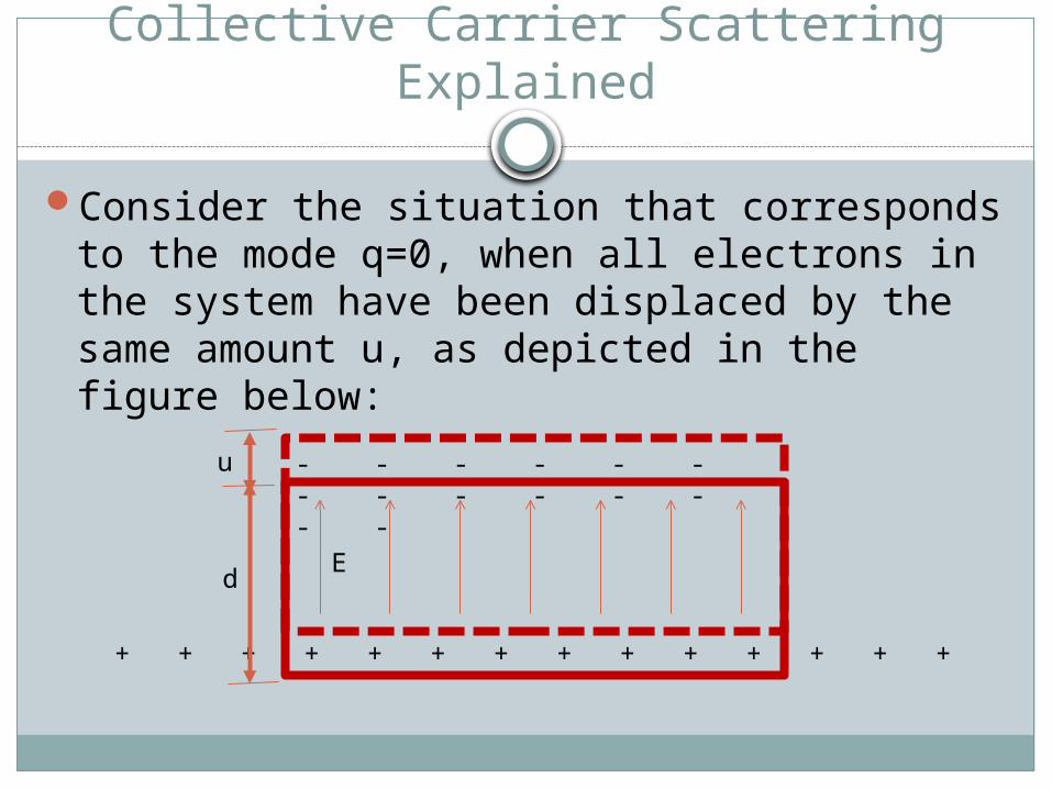
Consider the situation that corresponds to the mode q=0, when all electrons in the system have been displaced by the same amount u, as depicted in the figure below:

+ + + + + + + + + + + + + +

- - - - - - - - - - - - - -

u

dE

Collective Carrier Scattering Explained

Because of the positive (negative) surface charge density at the bottom (top) slab, an electric field is produced inside the slab. The electric field can be calculated using a simple parallel capacitor model for which:

The equation of motion of a unit volume of the electron gas of concentration n is:

neuE

Ed

neuA

V

Q

d

AC

appl

uen

neEdt

udnm

22

2

2

*

2/122

2

2

*,0

m

neu

dt

udpp

Collective Carrier Scattering Explained

Comments: Plasma oscillation is a collective longitudinal

excitation of the conduction electron gas. A PLASMON is a quantum of plasma oscillations.

PLASMONS obey Bose-Einstein statistics. An electron couples with the electrostatic field

fluctuations due to plasma oscillations, in a similar manner as the charge of the electron couples to the electrostatic field fluctuation due to longitudinal POP.

Collective Carrier Scattering Explained

The process is identical to the Frӧhlich interaction if plasmon damping is neglected. Then:

Note on qmax: Large qmax refers to short-wavelength oscillations, but one

Debye length is needed to screen the interaction. Therefore, when qmax exceeds 1/LD, the scattering should be treated as binary collision. qc=min(qmax,1/LD)

em

em

ab

abp

q

qN

q

qN

k

em

k min

max0

min

max02

2

ln)1(ln4

*

)(

1

Collective Carrier Scattering Explained

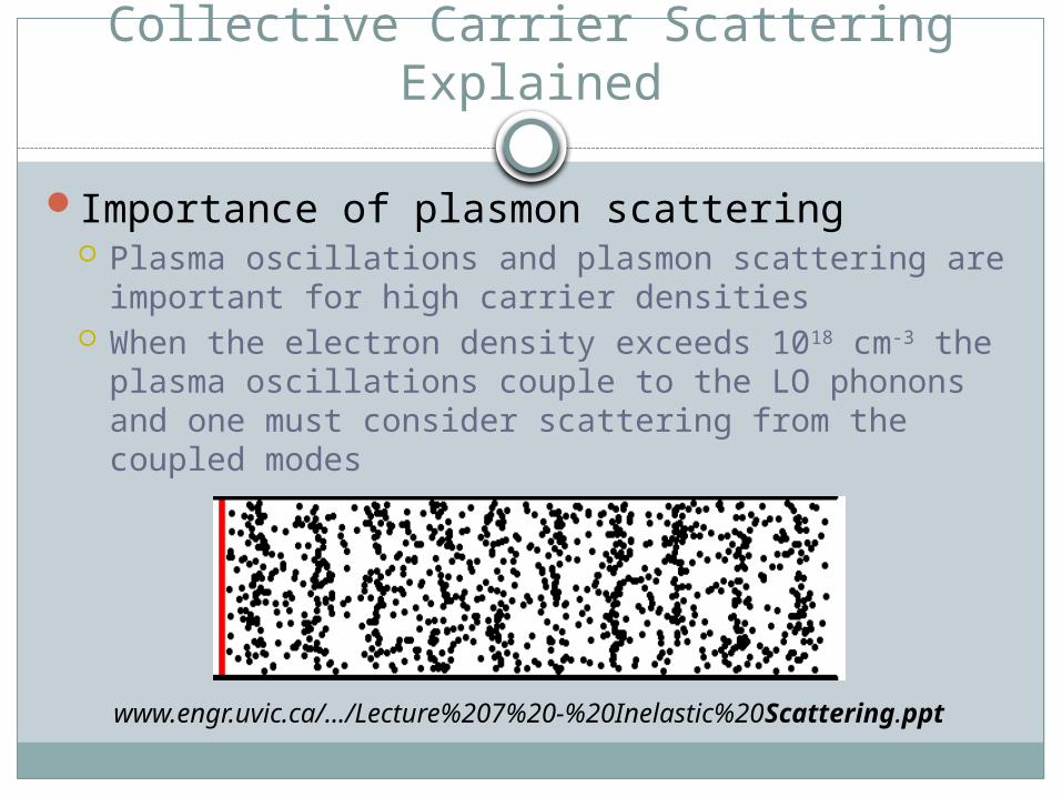
Importance of plasmon scattering Plasma oscillations and plasmon scattering are

important for high carrier densities When the electron density exceeds 1018 cm-3 the

plasma oscillations couple to the LO phonons and one must consider scattering from the coupled modes

www.engr.uvic.ca/.../Lecture%207%20-%20Inelastic%20Scattering.ppt

Electron-Electron Interactions(Binary Collisions)

This scattering mechanism is closely related to charged impurity scattering and the interaction between the electrons can be approximated by a screened Coulomb interaction between point-like particles, namely:

Then, one can obtain the scattering rate in the Born approximation as one usually does in Brooks-Herring approach.

DLree e

r

erH /

12

2

1212

4)(

Binary Collissions

To write the collision term, one needs to define a pair transition rate S(k1,k2,k1’,k2’), which represents the probability per unit time that electrons in states k1 and k2 collide and scatter to states k1’ and k2’, as shown diagramatically in the figure below:

k1k2

k2’k1’

r1 r2

Binary Collisions, Cont’d

The pair transition rate is defined as:

Since the interaction potential depends only upon the distance between the particles, it is easier to calculate M12 in a center-of-mass coordinate system, to get:

2112'2112

212'2'121

,)(,

2),,,(

21'2'1

kkrHkkM

EEEEMkkkkS

ee'

kkkk

2'1212

222

2

12 kk ,/1

1

q

LqV

eM

D

Binary Collisions Scattering Rate

To evaluate the scattering rate due to binary carrier-carrier scattering, one weights the pair transition rate that a target carrier is present and by the probability that the final states k1’ and k2’ are empty:

Note that a separate sum over k1’ is not needed because of the momentum conservation -function. For non-degenerate semiconductors, we have:

'2 2

)](1)][(1)[(),,,()(

1'2'12'2'121

1 k k

kfkfkfkkkkSk

'2 2

)(),,,()(

12'2'121

1 k k

kfkkkkSk

Binary Collisions Scattering Rate

In summary:

2221

223

24

21 /14

*)(

)(

1

2 D

D

k Lkk

kkLnemkf

k

Incorporation of the electron-electron interactions in EMC codes

For two-particle interactions, the electron-electron (hole-hole, electron-hole) scattering rate may be treated as a screened Coulomb interaction (impurity scattering in a relative coordinate system). The total scattering rate depends on the instantaneous distribution function, and is of the form:

22

02

0

k23

4

0kk

kkkk f

V

emnee

Screening constant

There are three methods commonly used for the treatment of the electron-electron interaction:

A. Method due to Lugli and FerryB. Rejection algorithmC. Real-space molecular dynamics

• This method starts form the assumption that the sum over the distribution function is simply an ensemble average of a given quantity.

• In other words, the scattering rate is defined to be of the form:

• The advantages of this method are:

1. The scattering rate does not require any assumption on the form of the distribution function

2. The method is not limited to steady-state situations, but it is also applicable for transient phenomena, such as femtosecond laser excitations

• The main limitation of the method is the computational cost, since it involves 3D sums over all carriers and the rate depends on k rather on its magnitude.

N

i Di

iDnee

L

Lenm

1 2223

24

01kk

kk

4k

/

(A) Method Due to Lugli and Ferry

• Within this algorithm, a self-scattering mechanism, internal to the interparticle scattering is introduced by the following substitution:

• When carrier-carrier collision is selected, a counterpart electron is chosen at random from the ensemble.

• Internal rejection is performed by comparing the random number with:

DD LL 2

1

1kk

kk22

0

0

/

220

0

1kk

kk

DL/

(B) Rejection Algorithm

• If the collision is accepted, then the final state is calculated using:

where:

The azimuthal angle is then taken at random between 0 and 2.

• The final states of the two particles are then calculated using:

)',(,)(

cos gg anglewhereLrg

rr

Dr

22 11

21

'''; 00 kkg kkg

ggkk

ggkk

'

'

'

'

2121

0

00

BULK SYSTEMSSEMICONDUCTOR DEVICE MODELING

Real-Space Treatment of the Electron-Electron

Interactions

Bulk Systems

(C)Real-space molecular dynamics

• An alternative to the previously described methods is the real-space treatment proposed by Jacoboni.

• According to this method, at the observation time instant ti=it, the total force on the electron equals the sum of the interparticle coulomb interaction between a particular electron and the other (N-1) electrons in the ensemble.

• When implementing this method, several things need to be taken into account:1. The fact that N electrons are used to represent a carrier density n = N/V means that a simulation volume equals V = N/n.

2. Periodic boundary conditions are imposed on this volume, and because of that, care must be taken that the simulated volume and the number of particles are sufficiently large that artificial application from periodic replication of this volume do not appear in the calculation results.

• Using Newtonian kinematics, the real-space trajectories of each particle are represented as:

and:

Here, F(t) is the force arising from the applied field as well as that of the Coulomb interaction:

• The contributions due to the periodic replication of the particles inside V in cells outside is represented with the Ewald sum:

2

21

tm

ttttt

*)(

)()(F

vrr

tm

tttt

*)(

)()(F

vv

iitqt )()( rEF

N

iii

i Ve

t1

2

2

321

4ra

rF )(

Simulation example of the role of the electron-electron interaction:

• The effect of the e-e scattering allows equilibrium distribution function to approach Fermi-Dirac or Maxwell Boltzmann distribution.

• Without e-e, there is a phonon ‘kink’ due to the finite energy of the phonon

Semiconductor Device Modeling

Ways of accounting for the short-range Coulomb interactions

Long-range Coulomb interactions are accounted for via the solution of the Poisson equation which gives the so-called Hartree term

If the mesh is infinitely small, the full Coulomb interaction is accounted for

However this is not practical as infinite systems of algebraic equations need to be solved

To avoid this difficulty, a mesh size that satisfies the Debye criterion is used and the proper correction to the force used to move the carriers during the free-flight is added

Earlier Work – k-space treatment of the Coulomb interaction

Good for 2D device simulationsRequires calculation of the distribution

function to recalculate the scattering rate at each time step and the screening which is time consuming

Implemented in the Damocles device simulator

K-space Approach

Present trends – Real-space treatment

Requires 3D device simulator, otherwise the method fails

There are several variants of this method Corrected Coulomb approach developed by Vasileska

and Gross Particle-particle-particle-mesh (p3m) method by

Hockney and Eastwood Fast Multipole method

Real Space Treatment Cont’d

Corrected Coulomb approach and p3m method are almost equivalent in philosophy

FMM is very different

Treatment of the short-range Coulomb interactions using any of these three methods accounts for: Binary collisions + plasma (collective) excitations Screening of the Coulomb interactions Scattering from multiple impurities at the same time

which is very important at high substrate doping densities

1. Corrected Coulomb approach

A resistor is first simulated to calculate the difference between the mesh force and the true Coulomb force

Cut-off radius is defined to account for the ions (inner cut-off radius)

Outer cut-off radius is defined where the mesh force coincides with the Coulomb force

Correction to the force is made if an electron falls between the inner and the outer radius

The methodology has been tested on the example of resistor simulations and experimental data are extracted

Corrected Coulomb Approach Explained

Resistor Simulations

MOSFET: Drift Velocity and Average Energy

2. p3m Approach

Details of the p3m Approach

Impurity located at the very source-end, due to the availability of Increasing number of electrons screening the impurity ion, has reduced impact on the overall drain current.

0%

10%

20%

30%

40%

50%

60%

0 10 20 30 40 50

Distance Along the Channel [nm]

Cur

rent

Red

uctio

n

Impurity position varying along the center of the channel

V G = 1.0 V

V D = 0.2 V

Source end Drain end

3. Fast Multipole Method

Different strategy is employed here in a sense that Laplace equation (Poisson equation without the charges) is solved. This gives the ‘Hartree’ potential.

The electron-electron and electron-ion interactions are treated using FMM

The two contributions are added togetherMust treat image charges properly. Good

news is that the surfaces are planar and the method of images is a good choice

Idea

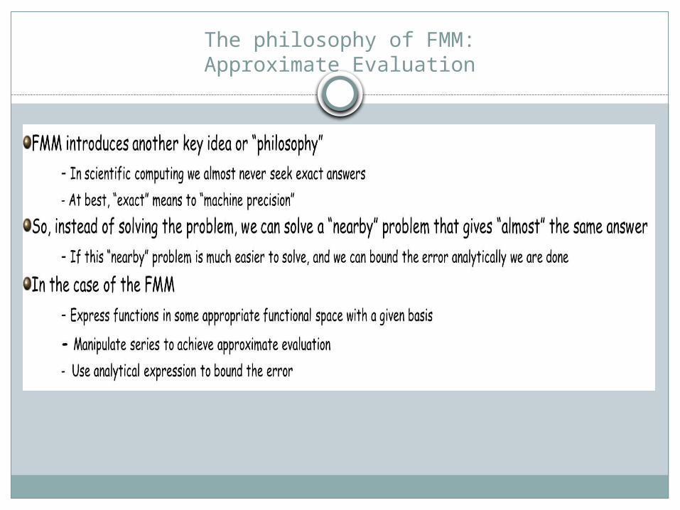
The philosophy of FMM:Approximate Evaluation

Ideology behind FMM

Simulation Methodology

Method of Images

Resistor Simulations

EXCHANGE-CORRELATION EFFECTSSCREENING OF THE COULOMB

INTERACTION POTENTIAL

More on the Electron-Electron Interactions for

Q2D Systems

Exchange-Correlation Correction to the Ground State

Energy if the System

Space Quantization

• Poisson equation:

d2VH

(z)dz2

=e2

esc

n(z)+Na(z)[ ]

• Hohenberg-Kohn-Sham Equation: (Density Functional Formalism)

Finite temperature generalizationof the LDA (Das Sarma and Vinter)

Veff

(z)=VH

(z)+Vxc

(z)+Vim

(z)

-h2

2mz*

¶2

¶z 2 +Veff (z) y n (z)=en y n (z)[ ]

EF

VG>0

e0

e1

e2

e3 e0

’

e1

’

z-axis [100](depth)

[100]-orientation:D2-band : mz=ml=0.916m0, mxy=mt=0.196m0

D4-band: mz=mt, mxy= (ml mt)

1/2

D2-band

D4-band

Exchange-Correlation Effects

E=EHF +Ecorr=EkinHF +Eexchange

HF +Ecorr

Total Ground StateEnergy of the System

Hartree-Fock Approximationfor the Ground State Energy

Accounts for the error madewith the Hartree-Fock Approximation

Accounts for the reductionof the Ground State Enerydue to the inclusion of thePauli Exclusion Principle

Ways of Incorporating the Exchange-Correlation Effects:

Density-Functional Formalism (Hohenberg, Kohn and Sham)

Perturbation Method (Vinter)

Ways of Incorporating the Exchange-Correlation Effects:

Density-Functional Formalism (Hohenberg, Kohn and Sham)

Perturbation Method (Vinter)

Subband StructureImportance of Exchange-Correlation Effects

Exchange-Correlation Correction:

Lower subband energies Increase in the subband

separation Increase in the carrier

concentration at which the Fermi level crosses into the second subband

Contracted wavefunctions

Vasileska et al., J. Vac. Sci. Technol. B 13, 1841 (1995)(Na=2.8x1015 cm-3, Ns=4x1012 cm-2, T=0 K)

Thick (thin) lines correspond to thecase when the exchange-correlationcorrections are included (omitted) inthe simulations.

0.02

0.06

0.1

0.14

0.18

0 20 40 60 80 100

second subband

first subband

Veff

(z)

Normalized wavefunction

Distance from the interface [Å]

Subband StructureComparison with Experiments

0

10

20

30

40

50

60

0 5x10 11 1x10 12 1.5x10 12 2x10 12 2.5x10 12 3x10 12

Exp. data [Kneschaurek et al.]V

eff(z)=V

H(z)+V

im(z)+V

exc(z)

Veff

(z)=VH(z)

Veff

(z)=VH(z)+V

im(z)

Ene

rgy

E10

[meV

] T = 4.2 K, Ndepl

=1011 cm-2

Ns [cm-2]

Kneschaurek et al., Phys. Rev. B 14, 1610 (1976) Infrared Optical AbsorptionExperiment:

far-ir

radiation

LED

SiO2 Al-Gate

Si-Sample

Vg

Transmission-Line Arrangement

Subband StructureComparison with Experiments

0

10

20

30

40

50

0 5x10 11 10 12 1.5x10 12 2x10 12 2.5x10 12 3x10 12

10 subb. appr. with Vxc

(z)

5 subb. appr. with Vxc

(z)

Hartree approximation

10 [

meV

]

Ns [cm-2]

Experimental data[Schäffler et al.]

T = 300 K

Ndepl

= 6x1010 [cm-2]

Unprimed ladder Primed ladder

Experimental data from: F. Schäffler and F. Koch (Solid State Communications 37, 365, 1981)

0

10

20

30

40

50

0 5x10 11 10 12 1.5x10 12 2x10 12 2.5x10 12 3x10 12

10 subb. appr. with Vxc

(z)

5 subb. appr. with Vxc

(z)

Hartree approximationDas Sarma and Vinter

1'0'

[m

eV]

Ns [cm-2]

Experimental data[Schäffler et al.]

T = 300 K

Ndepl

= 6x1010 [cm-2]

Screening of the Coulomb Interaction

What is Screening?

+

-

--

-

-

-

--

-

lD - Debye screening length

Ways of treating screening:

• Thomas-Fermi Methodstatic potentials + slowly varying in space

• Mean-Field Approximation (Random Phase Approximation)time-dependent and not slowly varying in space

r

3D: 1r

1rexp -

rlD

æ

è ç

ö

ø÷

screeningcloud

Example:

Diagramatic Description of RPAPolarization Diagrams

= + + + . . .

=1 -

Effective interaction (or ‘dressed’ or ‘renormalized’)

Bare interaction

= + + + . . .

bare pair-bubble

Proper (‘irreducible’)polarization parts

Screening:Simulation results are for: Na=1015 cm-3, Ns=1012 cm-

2

0

5x10 5

1x10 6

1.5x106

2x10 6

2.5x106

3x10 6

0 5x10 6 1x10 7 1.5x107 2x10 7

q00

(q)

q11

(q)

q0'0'

(q)

s

wavevector [cm-1]

s

s

0

0.2

0.4

0.6

0.8

1

1.2

0 2x10 6 4x10 6 6x10 6 8x10 6 1x10 7

T = 0 KT = 10 KT = 40 KT = 80 KT = 300 K

Wavevector [cm-1]

Relative Polarization Function:

P00(0)(q,0)/ P00

(0)(0,0)

Screening Wavevectors:

qnms (q,0)= - e2

2kPnm

(0)(q,0)

T=300 K

2D-Plasma Frequency: pl(q)e2Nsq2kmxy

*

Screening:Form-Factors: Na=1015 cm-3, Ns=1012 cm-2

10 -4

10 -3

10 -2

10 -1

0 5x106 1x10 7 1.5x107 2x10 7

|F01,00

|

|F01,11

|

|F01,01

|

|F01,0'0'

|

wavevector [cm-1]

10 -3

10 -2

10 -1

100

0 5x10 6 107 1.5x107 2x10 7

|F00,00

|

|F00,11

|

|F11,11

|

|F00,0'0'

|

|F11,0'0'

|

wavevector [cm-1]

Diagonal form-factors Off-diagonal form-factors

Fij,nm(q)= dz dz'0

¥

ò0

¥

ò y j*(z)y i(z)˜ G (q,z,z')ym

* (z')yn(z') =>i n

mjz'z