electromagnetic wave interaction with the auroral plasma - metabunk
TRANSCRIPT
University of California
Los Angeles
Electromagnetic Wave Interaction with the
Auroral Plasma
A dissertation submitted in partial satisfaction
of the requirements for the degree
Doctor of Philosophy in Physics
by
Jacqueline Tze-Ho Pau
2003

c° Copyright by
Jacqueline Tze-Ho Pau
2003

The dissertation of Jacqueline Tze-Ho Pau is approved.
Francis Chen
Steven Cowley
Warren Mori
Ralph Wuerker
Alfred Y. Wong, Committee Chair
University of California, Los Angeles
2003
ii
Table of Contents
1 Introduction . . . . . . . . . . . . . . . . . . . . . . . . . . . . . . . . 1
1.1 The Earth’s Ionosphere . . . . . . . . . . . . . . . . . . . . . . . . 1
1.2 Structure of the Ionosphere . . . . . . . . . . . . . . . . . . . . . 3
1.3 Propagation of Waves in the Ionosphere . . . . . . . . . . . . . . 9
1.4 Mode Conversion and Formation of Caviton . . . . . . . . . . . . 12
1.5 Stimulated Electromagnetic Emissions . . . . . . . . . . . . . . . 13
1.6 Previous Work . . . . . . . . . . . . . . . . . . . . . . . . . . . . 17
1.7 Outline of Thesis . . . . . . . . . . . . . . . . . . . . . . . . . . . 19
2 Experimental Setup . . . . . . . . . . . . . . . . . . . . . . . . . . . 21
2.1 Experimental Facilities . . . . . . . . . . . . . . . . . . . . . . . . 21
2.2 Diagnostics Techniques . . . . . . . . . . . . . . . . . . . . . . . . 27
2.2.1 HF Receiver . . . . . . . . . . . . . . . . . . . . . . . . . . 27
2.2.2 SEE Receiver . . . . . . . . . . . . . . . . . . . . . . . . . 29
2.2.3 Background Diagnostics . . . . . . . . . . . . . . . . . . . 31
2.3 Conditions for the Experiment . . . . . . . . . . . . . . . . . . . . 35
3 Reflected EM Wave under Matching Condition . . . . . . . . . 36
3.1 Spreading of the Ionosonde Echo Returns . . . . . . . . . . . . . . 36
3.1.1 Setup of the Dynasonde . . . . . . . . . . . . . . . . . . . 36
3.1.2 Experimental Results . . . . . . . . . . . . . . . . . . . . . 37
3.1.3 Discussions . . . . . . . . . . . . . . . . . . . . . . . . . . 40
iii

3.2 Comparison Between X- and O-Mode Heating . . . . . . . . . . . 41
3.2.1 Experimental Results . . . . . . . . . . . . . . . . . . . . . 43
3.2.2 Discussions . . . . . . . . . . . . . . . . . . . . . . . . . . 51
3.3 Conclusions . . . . . . . . . . . . . . . . . . . . . . . . . . . . . . 54
4 Spectral Structure of SEE under Matching Condition . . . . . 56
4.1 High Power Pumping . . . . . . . . . . . . . . . . . . . . . . . . . 56
4.1.1 Experimental Results . . . . . . . . . . . . . . . . . . . . . 56
4.1.2 Discussion . . . . . . . . . . . . . . . . . . . . . . . . . . . 62
4.2 The Effect of Preconditioning on Low Power Pumping . . . . . . . 66
4.2.1 Experimental Procedure . . . . . . . . . . . . . . . . . . . 66
4.2.2 Experimental Results . . . . . . . . . . . . . . . . . . . . . 68
4.2.3 Discussion . . . . . . . . . . . . . . . . . . . . . . . . . . . 78
4.3 Conclusion . . . . . . . . . . . . . . . . . . . . . . . . . . . . . . . 79
5 Spectral Structure of SEE at 2fce . . . . . . . . . . . . . . . . . . . 80
5.0.1 Experimental Results . . . . . . . . . . . . . . . . . . . . . 80
5.0.2 Discussion . . . . . . . . . . . . . . . . . . . . . . . . . . . 81
5.0.3 Conclusion . . . . . . . . . . . . . . . . . . . . . . . . . . . 89
6 Summary and Suggestions for Future Research . . . . . . . . . . 91
A Reprint of “Controlled ionospheric preconditioning and stimu-
lated electromagnetic radiation” by P. Y. Cheung, A. Y. Wong, J.
Pau, and E. Mjølhus, Phys. Rev. Lett., 80, 4891—4 (1998) . . . . . 96
iv

References . . . . . . . . . . . . . . . . . . . . . . . . . . . . . . . . . . . 101
v

List of Figures
1.1 The earth’s atmospheric temperature profiles calculated from the
MSIS-E-90 Atmospheric Model at HIPAS, Alaska. . . . . . . . . . 2
1.2 Various layers of the ionosphere. Actual electron density profiles
vary over a wide range and depend markedly on time of day, season,
sun-spot number and whether or not the ionosphere is disturbed. 4
1.3 Neutral density profiles calculated from the MSIS-E-90 Atmospheric
Model for both solar maximum and solar minimum period at HIPAS. 5
1.4 Atomic, and molecular ion profiles calculated from the Interna-
tional Reference Ionosphere IRI-2001 model for both solar maxi-
mum and solar minimum period at HIPAS. . . . . . . . . . . . . . 6
1.5 The ray paths computed from a cold-plasma theory. The Earth’s
magnetic field makes an angle of 13◦ with the density gradient at
HIPAS. . . . . . . . . . . . . . . . . . . . . . . . . . . . . . . . . . 10
1.6 Cartoon of direct spectral measurement setup. . . . . . . . . . . . 15
1.7 Diagrams showing the four basic SEE features. . . . . . . . . . . . 16
2.1 Ionospheric Research Site Map. . . . . . . . . . . . . . . . . . . . 22
2.2 (Top) The layout of the HIPAS array with eight crossed dipole
antennas field. Each antenna is connected to a transmitter with a
total maximum output power of 800 kW. . . . . . . . . . . . . . 23
2.3 (Top) Beam pattern with antennas phased 30 deg off vertical. (Bot-
tom) Beam pattern with all 8 antennas in phase. . . . . . . . . . . 25
vi

2.4 Setup of the narrow band (8 kHz) HF receiver for monitoring the
skywave. . . . . . . . . . . . . . . . . . . . . . . . . . . . . . . . . 28
2.5 SEE receiver setup. . . . . . . . . . . . . . . . . . . . . . . . . . . 29
2.6 Fat dipole antenna. . . . . . . . . . . . . . . . . . . . . . . . . . . 30
2.7 Radar coverage area of the HLMS auroral radar. . . . . . . . . . . 34
3.1 The USU dynasonde receiving antenna array configuration. D is
typically 30 meters. . . . . . . . . . . . . . . . . . . . . . . . . . . 37
3.2 Ionogram obtained on October 3, 1992 at 05:01 UT (before match-
ing) by the Utah Dynasonde. (Top panel) The ionogram shows a
smooth F-layer return at a peak frequency 3.5 MHz. The solid
line indicates the pump frequency. (Bottom panel) Skymaps show
the scattering pattern of the O wave echo return. Geomagnetic
coordinate is used. . . . . . . . . . . . . . . . . . . . . . . . . . . 38
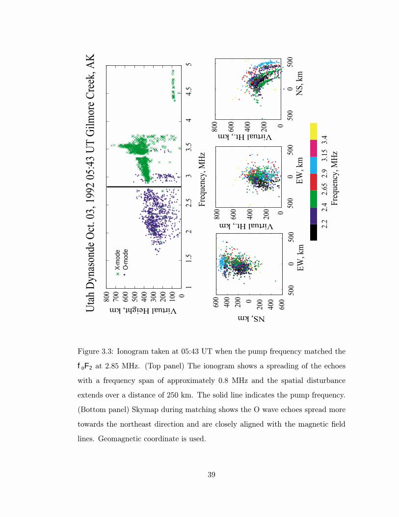
3.3 Ionogram taken at 05:43 UT when the pump frequency matched
the foF2 at 2.85 MHz. (Top panel) The ionogram shows a spread-
ing of the echoes with a frequency span of approximately 0.8 MHz
and the spatial disturbance extends over a distance of 250 km. The
solid line indicates the pump frequency. (Bottom panel) Skymap
during matching shows the O wave echoes spread more towards
the northeast direction and are closely aligned with the magnetic
field lines. Geomagnetic coordinate is used. . . . . . . . . . . . . . 39
3.4 The ray paths computed from a cold-plasma theory. The Earth’s
magnetic field makes an angle of 13◦ with the density gradient at
HIPAS. . . . . . . . . . . . . . . . . . . . . . . . . . . . . . . . . . 42
vii
3.5 Data obtained on March 9, 1995 showing the amplitude of the
reflected wave and the interpolated density profile generated from
the DISS during the experiments. The pump frequency was set at
2.85 MHz. . . . . . . . . . . . . . . . . . . . . . . . . . . . . . . . 44
3.6 Data obtained on March 22, 1995 showing the amplitude of the
reflected wave and the interpolated density profile generated from
the DISS during the experiments. Ionograms were taken only be-
fore and after possible matching condition. The pump frequency
was set at 4.53 MHz. . . . . . . . . . . . . . . . . . . . . . . . . . 45
3.7 A plot of the Doppler frequency shifts of the skywave return taken
on March 22, 1995. A net positive frequency shift is observed
from the O-mode heating and a negative shift from the X-mode
heating. The frequency shifts become more significant when the
heater frequency is close to fOF2 between 6:00 and 7:00 UT. The
pump frequency was set at 4.53 MHz. . . . . . . . . . . . . . . . . 47
3.8 A plot of FWHM of the reflected pump signals as function of time
for the data taken on February 17, 1995. CW O-mode heating
was used. The solid line shows the average halfwidth for every
five-minute interval. The pump frequency was set at 2.85 MHz. . 48
3.9 A plot of FWHM of the reflected pump signals as function of time
for the data taken on September 20, 1995. CW O-mode heating
was used. The solid line shows the average halfwidth for every
five-minute interval. The pump frequency was set at 2.85 MHz. . 49
viii

3.10 A plot of FWHM of the reflected pump signals as function of time
for the data taken on March 22, 1995. A halfwidth of 4—10 Hz was
observed when the heater frequency was close to foF2 between
03:45 and 04:45 UT. The solid and dashed lines show the average
for each O- and X-mode heating cycle, respectively. The pump
frequency was set at 4.53 MHz. . . . . . . . . . . . . . . . . . . . 50
4.1 Temporal evolution of the reflected pump wave at 4.53 MHz (top
panel) and the SEE signal at -10 kHz from fpump (bottom panel).
A gradual increase is observe in the bottom panel during the first
10 s. Data were taken at cold start. . . . . . . . . . . . . . . . . . 57
4.2 Temporal evolution of the reflected pump wave at 4.53 MHz (top
panel) and the SEE signal at -10 kHz from fpump. Strong overshoot
is observed immediately after turn-on. Data were taken during
high power heating after pre-heating the ionosphere. . . . . . . . . 59
4.3 Frequency spectra taken on November 17, 1997 at HIPAS with
fpump = 4.53 MHz under different values of foF2. The horizontal
scale is the frequency offset from 4.53 MHz. . . . . . . . . . . . . 60
4.4 Frequency spectra taken on March 24, 2001 at HAARP with fpump
= 5.9 MHz under different values of foF2. . . . . . . . . . . . . . . 61
4.5 Frequency spectra taken on March 24, 1999 at HAARP when foF2
was passing through fpump = 7.4 MHz from above. The vertical
scale is the offset from the start of the transmission. . . . . . . . . 63
4.6 Frequency spectra taken on March 14, 1997 at HIPAS when foF2
was a few 100 kHz below fpump = 4.56 MHz. . . . . . . . . . . . . 64
ix

4.7 (a) Heating schemes used during the pre-conditioning experiments
and (b) detailed procedure for the low power heating sequence. . . 67
4.8 Frequency spectra taken on November 17, 1997 at HIPAS during
the T2 sequence under matching condition. The axes are the fre-
quency offset from 4.53 MHz and the time offset from the time the
H1 sequence is off. . . . . . . . . . . . . . . . . . . . . . . . . . . 69
4.9 Frequency spectra taken on November 17, 1997 at HIPAS during
the T2 sequence under overdense condition. The axes are the
frequency offset from 4.53 MHz and the time offset from the time
the H1 sequence is off. . . . . . . . . . . . . . . . . . . . . . . . . 70
4.10 Temporal variation in intensity of SEE signal at 10 kHz below
each test frequency during T2 transmission at (a) matching and (b)
overdense condition. The signal is more steady and stronger when
matched and gradually decreased to noise level when overdense.
The average noise level is set to 0 dB. . . . . . . . . . . . . . . . . 72
4.11 Frequency spectra taken at 0.5 s after the turn on of the T2 se-
quence at 4.555 MHz under the matching (solid line) and overdense
condition (dotted line). . . . . . . . . . . . . . . . . . . . . . . . . 74
4.12 Frequency spectra taken on March 24, 2001 at HAARP during the
T2 sequence at 5.93 MHz. Data was taken when foF2 was about
6.1 MHz under the overdense condition. . . . . . . . . . . . . . . . 75
4.13 Frequency spectra taken on March 24, 2001 at HAARP during the
T2 sequence at 5.93 MHz. Data was taken when foF2 was about
6 MHz near the matching condition. . . . . . . . . . . . . . . . . 76
x

4.14 Frequency spectra taken on March 24, 2001 at HAARP during the
T2 sequence at 5.93 MHz. Data was taken when foF2 was about
5.8 MHz under the slightly underdense condition. . . . . . . . . . 77
5.1 A spectrogram taken on February 13, 2003 using the HIPAS heater
at 2.85 MHz during the 800 kW high power heating and 2.875 MHz
during the 100 kW low power heating. . . . . . . . . . . . . . . . 82
5.2 A spectrogram taken on February 13, 2003 using the HIPAS heater
at 2.85 MHz during the 800 kW high power heating and 2.875 MHz
during the 50 kW low power heating. . . . . . . . . . . . . . . . 83
5.3 A spectrogram taken on February 13, 2003 using the HIPAS heater
at 2.85 MHz during the 800 kW high power heating and 2.875 MHz
during the 75 kW low power heating. . . . . . . . . . . . . . . . 84
5.4 A spectrogram taken on March 27, 2003 during the frequency step-
ping between 2.85 and 2.88 MHz. Both stepping up and down are
shown. Sidebands are observed between 2.851 and 2.860 MHz. . 85
5.5 Spectrogram taken on March 27, 2003 during the frequency step-
ping between 2.85 and 2.88 MHz. Both stepping up and down are
shown. Sidebands are observed between 2.872 and 2.880 MHz. . 86
5.6 A spectrogram taken on March 28, 2003 during the transmitter
stepping experiments. The pump frequency was at 2.88 MHz. . . 87
5.7 Second harmonics of the ionospheric electron cyclotron frequency
versus height at HIPAS. . . . . . . . . . . . . . . . . . . . . . . . 90
xi
6.1 Block diagram of a self-consistent physical model to explain the results
of EM wave interact with the ionosphere at the peak of the ionospheric
density profile. The model includes the initial conditions, heating ef-
fects, and experimental observations. . . . . . . . . . . . . . . . . . 93
xii

List of Tables
2.1 HIPAS operating parameters (Absorption is neglected). . . . . . . 24
2.2 Parameters of the HAARP antenna array. . . . . . . . . . . . . . 26
xiii

Acknowledgments
I would like to acknowledge the many and important people behind the scenes
that have made this thesis possible. First, I would like to give thanks to God
for He has given me strength, wisdom, and endurance. As printed in the Bible,
the Book of Philippians 4:13, ”I can do everything through Him who gives me
strength”.
I would like to express my deepest gratitude to my thesis advisor, Professor
Alfred Wong, for giving me the opportunity to engage in this research, for his
support, guidance, and patience with me.
I am grateful to the staff of the HIPAS Observatory and the HAARP facility
for their all-time supports in performing the experiments, without which, this
thesis could not be completed.
I would like to acknowledge many fruitful conversations and insightful sug-
gestions from Dr. Ralph Wuerker, Dr. Peter Cheung, Dr. Thomas Leyser, Dr.
Glenn Rosenthal, and Dr. Viktor K. Decyk. They have helped me in an extent
more than they probably know.
I thank Dr. Terry Bullet for his collaboration in providing ionograms, Dr.
Bill Bristow and Dr. John M. Hughes for providing the SuperDARN data, Dr.
Paul Bernhardt and Dr. Craig Selcher for the support in using the NRL SEE
receiver.
Thanks also to all of my friends for their warmest friendship and belief in me
at all times. Their friendship and encouragement have helped me to live through
all the ups and downs throughout the course of this project.
Last but not least, I would like to thank my family for their patience, constant
support, incessant prayers for me, and for giving me the freedom to pursue my
xiv
interest.
This research was supported by the Office of Naval Research. The HIPAS
Observatory is operated by the University of California, Los Angeles and is fi-
nancially supported by the Office of Naval Research. The HAARP facility is
managed jointly by the Air Force Research Laboratory and the Office of Naval
Research.
The article in the appendix is reprinted with the permission of the publisher:
-P. Y. Cheung, A. Y. Wong, J. Pau, and E. Mjølhus, Physical Review Letters,
Vol.80, 4891-4 (1998). Copyright 1998 by the American Physical Society.
xv

Vita
1968 Born, Hong Kong
1990 B.S. (Physics) and B.S. (Applied Mathematics), UCLA, Los
Angeles, California.
1992 M.S. (Physics), UCLA, Los Angeles, California.
1994—2002 Research Assistant, Department of Physics and Astronomy,
UCLA.
Publications and Presentations
B. Song, A. Y. Wong, J. Villasenor, G. Rosenthal, M. McCarrick, J. Pau, and
D. Sentman, Experimental study of double resonance parametric excitations in
the ionosphere Radio Sci., 30, 1875—83 (1995).
J. Pau, A. Y. Wong, J. Villasenor, B. Song, and H. Zwi, Matching the critical
plasma frequencies in the ionosphere with the HIPAS heater array, Paper
presented at the meeting of the High Power RF Ionospheric Modification
Workshop, Santa Fe, New Mexico, April 1995.
xvi
J. Pau, A. Y. Wong, G. Rosenthal, J. Villasenor, and B. Song, Generation of
density perturbations by frequency matching at the peak of the ionospheric
density profile,
J. Pau, J. Villasenor, H. R. Zwi, B. Song, E. Nichols, A. Y. Wong, and T.
Tanikawa, Preliminary results on HIPAS imaging riometer ionospheric studies,
Paper presented at the Fall meeting of the High Power RF Ionospheric
Modification Workshop, Santa Fe, New Mexico, April 1996.
Paper presented at the Fall meeting of the High Power RF Ionospheric
Modification Workshop, Santa Fe, New Mexico, April 1996.
J. Pau, A. Y. Wong, J. Villasenor, T. Berkey, and L. C. Tsai, Generation of
Large Density Perturbations by Frequency Matching at the Peak of the
Ionospheric Density Profile, Paper presented at the meeting of the 26th Annual
Anomalous Absorption Conference, Fairbanks, Alaska, August 1996.
J. Pau, J. Villasenor, H. R. Zwi, B. Song, A.Y. Wong, and T. Tanikawa,
Preliminary Results on HIPAS Imaging Riometer Ionospheric Studies, Paper
presented at the meeting of the 26th Annual Anomalous Absorption
Conference, Fairbanks, Alaska, August 1996.
J. Pau, A. Y. Wong, J. Villasenor, P. Y. Cheung, T. Berkey, and L. C. Tsai,
Observations of HF Ionospheric Modification at the Peak of the Ionospheric
Density Profile, Paper presented at the Fall meeting of the American
Geophysical Union (AGU), San Francisco, California, December 1996.
xvii

J. Villasenor, A. Y. Wong, B. Song, J. Pau, M. McCarrick, and D. Sentman
Comparison of ELF/VLF generation modes in the ionosphere by the HIPAS
heater array Radio Sci., 31, 211—26 (1996).
J. Pau, P. Y. Cheung, A.Y. Wong, and W. T. Armstrong, Beat Wave Heating of
the F-Layer Auroral Ionosphere, Paper presented at the meeting of the RF
Ionospheric Interactions Workshop, Santa Fe, New Mexico, April 1997.
J. Pau, H. Zwi, A. Y. Wong, R. Wuerker , and P.Y. Cheung Recent Results on
ELF Excitations at HIPAS, Paper presented at the meeting of the RF
Ionospheric Interactions Workshop, Santa Fe, New Mexico, April 1997.
P. Y. Cheung, E. Mjølhus, D. F. DuBois, J. Pau, H. Zwi, and A. Y. Wong,
Stimulated radiation from strong Langmuir turbulence in ionospheric
modification, Phys. Rev. Lett., 79, 1273—6 (1997).
J. Pau, A. Y. Wong, and P. Y. Cheung, Observations of HF Ionospheric
Pre-conditioning near foF2, Paper presented at the meeting of the RF
Ionospheric Interactions Workshop, Santa Fe, New Mexico, April 1998.
P. Y. Cheung, A. Y. Wong, J. Pau, and E. Mjølhus, Controlled ionospheric
preconditioning and stimulated electromagnetic radiation, Phys. Rev. Lett., 80,
4891—4 (1998).
P. Y. Cheung, J. Pau, and W. T. Armstrong, Dual-site ionospheric modification
experiments, Paper presented at the meeting of the RF Ionospheric Interactions
xviii

Workshop, Santa Fe, New Mexico, April 1999.
J. Pau, P. Y. Cheung, and A. Y. Wong, SEE experiments at HAARP, Paper
presented at the meeting of the RF Ionospheric Interactions Workshop, Santa
Fe, New Mexico, April 1999.
J. Pau, A. Y. Wong, and P. Y. Cheung, Optimization of Ionospheric
Modification near the Peak of the Ionospheric Density Profile, Paper presented
at the 41st Annual Meeting of the American Physical Society Division of
Plasma Physics, Seattle, Washington, November 1999.
A. Y. Wong and J. pau, Generation of ELF/VLF Using Frequency Sweeping
Method, Paper presented at the meeting of the RF Ionospheric Interactions
Workshop, Santa Fe, New Mexico, April 2000.
J. Pau, T.B. Leyser, and A. Y. Wong, Effects of Preconditioning of HAARP
Interaction near foF2, Paper presented at the meeting of the RF Ionospheric
Interactions Workshop, Santa Fe, New Mexico, April 2001.
J. Pau, A. Y. Wong, R. Wuerker, V. K.Decyk, and T. B. Leyser, Generation of
Vertical Current and ELF/VLF by Controlled Frequency sweep of HAARP,
Paper presented at the 43rd Annual Meeting of the American Physical Society
Division of Plasma Physics, Long Beach, California, November 2001.
L-C. Tsai, F. T. Berkey, A. Y. Wong, and J. Pau, Dynasonde observations of
ionospheric modification experiments with the HIPAS observatory, J. Atmos.
xix

Sol. Terr. Phys., 63, 107—16 (2001).
J. Pau and A. Y. Wong, E. A. Gerken, U. S. Inan, and W. Bristow, SEE and
Radar Observations during the February 2002 HAARP Optical Campaign,
Paper presented at the meeting of the RF Ionospheric Interactions Workshop,
Santa Fe, New Mexico, April 2002.
J. Pau, A. Y. Wong, G. Rosenthal, K. E. Koziar, and K. Stone, Enhancement of
EM-Ionospheric Interaction through Plasma Lens and Frequency Chirping,
Paper presented at the 44th Annual Meeting of the American Physical Society
Division of Division of Plasma Physics, Orlando, Florida, November 2002.
J. Pau and A. Y. Wong, SEE at near 2nd gyroharmonics, Paper presented at
the meeting of the RF Ionospheric Interactions Workshop, Santa Fe, New
Mexico, April 2003.
xx
Abstract of the Dissertation
Electromagnetic Wave Interaction with the
Auroral Plasma
by
Jacqueline Tze-Ho Pau
Doctor of Philosophy in Physics
University of California, Los Angeles, 2003
Professor Alfred Y. Wong, Chair
High power radio electromagnetic waves interaction with the auroral plasma have
been investigated. Plasma in this auroral region can be illuminated by EM waves
for a prolonged period of time and thus, experience accumulative perturbations
and resonances because of its long plasma lifetime, slow transport rates, and weak
convection, especially near the peak of the ionospheric electron density profile. A
plasma resonance at a specific height in the ionosphere has a corresponding EM
wave frequency. These plasma resonances can enhance the local electromagnetic
fields, and therefore their interactions with plasma particles leading to turbu-
lences, local heating, density perturbations, and field aligned striations. These
effects are more pronounced when the EM wave frequency is near foF2, the fre-
quency for the resonance near the peak of the ionospheric electron density profile.
Optical emissions are also enhanced under such conditions.
The non-linear process at the resonance layer can stimulate emission of elec-
tromagnetic waves which appear as the sidebands of the reflected EMwave. When
the ionosphere is pre-conditioned first with high power EM wave, the threshold
level of this non-linear process is reduced. The spectral features of the sidebands
xxi

can then be excited with an effective radiation power (ERP) level of 24 dB less
than that normally required. In particular, pre-conditioning near the foF2 res-
onant layer can further enhance the non-linear process. At this layer, density
perturbation is stronger and can affect a larger region as the density scale length
is largest. Consequently, the density needs a longer time to recover.
This thesis also discusses the capability at the HIPAS facility and attempts to
study interactions at the second harmonic of the ionospheric electron cyclotron
frequency. This is the first investigation to date on this critical resonance. EM
waves from the ground facility can reach this layer without much loss by a mode
conversion from the right-circular to left-circular polarization. The plasma reso-
nance and the cyclotron resonance can now occur in the same layer. As a result,
new spectral features manifest in the sidebands of the reflected EM wave from
this layer. A simple model is introduced to explain the generation mechanism of
this new spectral feature.
xxii

CHAPTER 1
Introduction
1.1 The Earth’s Ionosphere
The ionosphere is an example of naturally occurring plasma formed by solar
photo-ionization and soft x-ray radiation. Ultraviolet radiation from the sun ion-
izes the atmospheric constituents. Free thermal (1 < eV ) electrons and ions are
present in the earth’s upper atmosphere between 50 km and 6000 km approxi-
mately. In this region, the atmospheric temperature first increases with altitude
to an overall maximum value (∼ 900 K) and then becomes constant with alti-
tude (see Figure 1.1). In the ionosphere, a balance between photo-ionization
and various loss mechanisms gives rise to an equilibrium density of free electrons
and ions with a horizontal stratified structure. The density of these electrons is
a function of the height above the earth’s surface and is dramatically affected by
the effects of sunrise and sunset, especially at the lower altitudes. The presence
of these free electrons in the ionosphere can influence the propagation of radio
waves.
In comparison with laboratory plasmas, the ionospheric plasma is long-lived
and effectively unbounded. The transport rate is low such that cumulative tur-
bulent and radiation effects can occur. As a result, a moderate power of approxi-
mately 1 MW can excite a wide range of temporal and spatial plasma instabilities.
At an altitude of 100 km, the energy flux is∼ 0.56mW/m2, neglecting ionospheric
1

100 200 300 400 500 600 700 800 900 10000
50
100
150
200
250
300
350
400
450
500
Temperature Profile
Daytime
Night time
Temperature (K)
Hei
ght (
Km
)
Figure 1.1: The earth’s atmospheric temperature profiles calculated from the
MSIS-E-90 Atmospheric Model at HIPAS, Alaska.
2

absorption. Even though the transmitted power is more powerful than that used
in the laboratory plasma experiments, this pumping energy is rather weak when
compared to the ionospheric plasma thermal energy. The ratio is on order of
10−4 — 10−3. The characteristic scale lengths of many plasma phenomena are
much smaller than the size of the ionospheric plasma, therefore experiments can
be conducted in a very homogeneous environment.
1.2 Structure of the Ionosphere
The ionosphere is conventionally divided into the D-, E-, and F-regions (see
Figure 1.2). The D-region lies between 60 and 95 km, the E-region between
95 and 150 km, and the F-region lies above 150 km. In daylight, it is possible
to distinguish two separate layers within the F-region, the F1 (lower) and the
F2 (upper) layers. During nighttime, these two layers combine into one single
layer. The combined effect of gravitationally decreasing densities of neutral atoms
and molecules and increasing intensity of ionizing solar ultra-violet radiation with
increasing altitudes (see Figure 1.3, 1.4) , gives a maximum plasma density during
daytime in the F-region at a few hundred kilometers altitude. During daytime,
the ratio of charged particles to neutral particles concentration can vary from
10−8 at 100 km to 10−4 at 300 km and 10−1 at 1000 km altitude.
The D-region is both a refracting and an absorbing medium for radio waves.
When a radio wave travels through the ionosphere, it interacts with the electrons
and sets them into oscillation. With the high concentration of both molecular
and atomic gas particles in the D-region, these oscillations are damped by colli-
sions between electrons and gas molecules. Throughout the D-region the collision
frequency decreases exponentially with height, roughly proportional to the neu-
tral gas pressure, whereas electron density increases rapidly with height. In this
3

0
100
200
300
400
500
600
700
800
900
1000
D
E
F
Day time
Night time
Hei
ght (
km)
Electrons/cm 3
Density Profile
2 3 4 5 610 10 10 10 10
Figure 1.2: Various layers of the ionosphere. Actual electron density profiles vary
over a wide range and depend markedly on time of day, season, sun-spot number
and whether or not the ionosphere is disturbed.
4

0
100
200
300
400
500Daytime (Solar Minimum)
Hei
ght (
Km
)
100 105 1010 1015 10200
100
200
300
400
500Night time (Solar Minimum)
Density (cm3
)
Hei
ght (
Km
)
0
100
200
300
400
500Daytime (Solar Maximum)
100 105 1010 1015 10200
100
200
300
400
500Night time (Solar Maximum)
ON2O2HeH
Density (cm3
)
Figure 1.3: Neutral density profiles calculated from the MSIS-E-90 Atmospheric
Model for both solar maximum and solar minimum period at HIPAS.
5

100
200
300
400
500Daytime (Solar Minimum)
Hei
ght (
Km
)
0 1 2 3x 10
5
100
200
300
400
500Night time (Solar Minimum)
Density (cm3
)
Hei
ght (
Km
)
100
200
300
400
500Daytime (Solar Maximum)
0 2 4 6
100
200
300
400
500Night time (Solar Maximum)
eO+O2
+
NO+
Density (cm3
)x 10
5
Figure 1.4: Atomic, and molecular ion profiles calculated from the International
Reference Ionosphere IRI-2001 model for both solar maximum and solar minimum
period at HIPAS.
6

region, chemical processes are most important, molecular ions dominate, and N2,
O2, and O are the most abundant neutral species. The electron density is sharply
reduced at night because molecular ions have a much higher recombination rate
with electrons than atomic ions. Thus, the linear absorption of radio waves in
this region varies from a typical 4 — 10 times (or 6 — 10 dB) during daytime to a
much lower rate during nighttime.
The behavior of the E-region is subject to close solar control. In this region,
the basic chemical reactions are not as complicated as those in the D-region.
The major ions are NO+, O+2 , and N
+2 . The total ion density is of the order of
105 cm−3, while the neutral density is greater than 1011 cm−3. Therefore, the
E-region plasma is weakly ionized, and collisions between charged particles are
not important. The sporadic E layer consists largely of relatively dense patches
of electrons with a horizontal extent of tens of kilometers and are thought to
be produced by meteoric particles. In addition to photo-ionization, energetic
particles from the solar wind collide with the neutral gas resulting in additional
plasma production in the E-region.
The F-region is much thicker than the E-region and heavily ionized, where
maximum electron density locates in the range 200 — 400 km. In this region, the
O+ and O atomic species dominate. In daylight, a subsidiary bulge is observed in
the curve of electron density just below the maximum. This is the F1-layer. The
layer where the main maximum electron density locates is the F2-layer. The F2-
layer’s maximum ionospheric electron plasma frequency is the critical frequency
“foF2”. The peak ion density in the F2-layer is roughly a factor of 10 greater
than that in the E-region, while the neutral density (108 cm−3) is still orders of
magnitude greater than the ion density. The plasma in this region is partially
ionized and collisions among charged and neutral particles must be taken into
7

account. The effective electron collision frequency is νe ∼ 500 Hz at 200 km
altitude and the thermal electron mean free path is about 1 km. The scale
height of the ambient plasma density profile is defined as the height differences
for the density to increase by a factor of e from its reference value. At the
bottom boundary of F-region, where the pump wave is reflected, the scale height
is typically 50 km. It is much larger than the vacuum pump wavelength of ∼ 30— 100 m.
Sunrise and sunset have little or no influence in the F-region. However, the
geomagnetic field plays an important role in the structure and dynamics of this
region. As charged particles collisions are sufficiently less frequent in this region,
the motion of charged particles is constrained by the earth’s magnetic field. At
high latitudes, where the geomagnetic field is nearly perpendicular to the earth’s
surface the field lines can extend into the interplanetary medium. Charged parti-
cles ejected from the sun are thus guided down into the ionosphere and depicted
as the aurora.
The electron distribution throughout these layers is subject to diurnal, daily,
seasonal, and geographical variations as well as the magnetic disturbance asso-
ciates with solar activities. Among these layers, the F2 layer is the most variable.
When a solar flare occurs, the sudden increase of x-ray emission will result in a
large increase of ionization in the lower D-, E- and F-regions of the ionosphere,
on the sunlit side of the earth. Sufficiently large or long-lived solar flares will
produce geomagnetic storms that may result in ionospheric disturbances.
The earth’s magnetic field varies partly due to the external currents and
the induced earth currents. “Quiet days” are days when the transient magnetic
variations are regular, while on ”disturbed” days they are magnetically disturbed.
During these disturbed days, additional currents circulate in the ionosphere. In
8
addition to the visible aurora, the ionization process is enhanced, corresponding
to the increase in sporadic E and D-region absorption.
1.3 Propagation of Waves in the Ionosphere
The presence of the earth’s magnetic field makes the ionosphere a double re-
fractive medium. When an electromagnetic (EM) wave of frequency fo from
the ground enters the ionospheric D-region its refraction depends on the initial
polarization state of the incident wave. Two types of waves are most commonly
used in the ionospheric modification experiments, namely ordinary (O-mode) and
extraordinary (X-mode) waves.
At high latitudes such as Alaska, the magnetic field is directed nearly vertically
downwards. When a right-handed circularly polarized (O-mode) pump wave
is propagating upwards which is anti-parallel to the earth’s magnetic field, its
polarization becomes left-handed after reflection in the ionosphere. An X-mode
pump has a polarization opposite to the O-mode pump and is the same direction
as an electron cyclotron rotation.
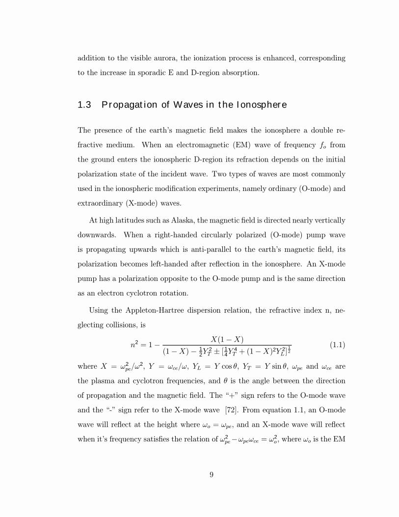
Using the Appleton-Hartree dispersion relation, the refractive index n, ne-
glecting collisions, is
n2 = 1− X(1−X)(1−X)− 1
2Y 2T ± [ 14Y 4
T + (1−X)2Y 2L ]
12
(1.1)
where X = ω2pe/ω
2, Y = ωce/ω, YL = Y cos θ, YT = Y sin θ, ωpe and ωce are
the plasma and cyclotron frequencies, and θ is the angle between the direction
of propagation and the magnetic field. The “+” sign refers to the O-mode wave
and the “-” sign refer to the X-mode wave [72]. From equation 1.1, an O-mode
wave will reflect at the height where ωo = ωpe, and an X-mode wave will reflect
when it’s frequency satisfies the relation of ω2pe−ωpeωce = ω2
o , where ωo is the EM
9

-2 -1 0 1 2 3 4 50
20
40
60
80
100
120
140
Distance (Km)
Heigh
t (Km
)
Ray paths for vertical incidence O and X rays
X Trace
O Trace
Earth's Magnetic Field
13 Dip Angleo
Figure 1.5: The ray paths computed from a cold-plasma theory. The Earth’s
magnetic field makes an angle of 13◦ with the density gradient at HIPAS.
wave frequency. Hence, an upward directed X-mode wave will reflect at a lower
altitude than an upward directed O-mode wave (Figure 1.5). The separation
of the O- and X-mode critical frequencies is approximately fce/2. Raytracing
calculations indicate that their ray paths are very different and well-separated
laterally [8].
The angle between the pump electric field and the ambient geomagnetic field
determines the nature of the plasma turbulence and the induced plasma waves.
Langmuir turbulence is most strongly excited in the plasma resonance region
parallel to the geomagnetic field. With the larger magnetic field angle at lower
latitudes the parallel electric field component remains parallel to the magnetic
10

field over a larger altitude range below the reflection height. Therefore, the
excitation of the Langmuir turbulence is more important in the lower latitudes.
Upper-hybrid (UH) turbulence occurs where the electric field is perpendicular to
the geomagnetic field. At higher latitudes, the UH resonance region is only a few
kilometers below the plasma resonance region.
Not only are there differences in the excitation locations, the physical processes
and temporal scales are also very different between the Langmuir and UH tur-
bulence. The Langmuir turbulence involves ponderomotive interactions between
the Langmuir and ion-acoustic oscillations whereas UH turbulence involves both
ponderomotive and transport processes. The Langmuir turbulence includes dy-
namics at the short time scale of electron fluctuations and at long time scale of
ion fluctuations. Meanwhile, the UH turbulence also includes the much slower
dynamics of transport processes.
A vertical incident pump wave is partially or totally reflected in the reflection
region of a monotonically increasing plasma density with height. The incident
and the reflected waves interact with each other and form a standing wave pattern
[61, 62]. As the pump wave approaches the reflection region, the wavelength of
the pump increases and the wave slows down. Because the energy flow must
be constant, the decrease in the wave velocity leads to an increase in the wave
amplitude. This is usually referred to as “swelling”. This swelling causes an
enhancement in the intensity of the pump wave electric field, and thus a tendency
towards the Langmuir turbulence. Swelling only occurs in the parallel component
of the electric field. Therefore, the maximum electric field strength is located
just below the reflection level where the pump electric field is almost parallel
to the geomagnetic field. The angle between the pump electric field and the
geomagnetic field increases below the reflection region. At the UH resonance
11

layer, the electric field is almost perpendicular to the geomagnetic field, thus
the perpendicular electric field intensity drops to minimum. When the pump
frequency approaches the critical frequency, the density gradient in the pump
reflection region decreases. The swelling now decreases but the vertical extent of
the pump—plasma interaction region increases, which affects the pump-induced
perturbations. The condition when the pump wave interacts strongly with the
region containing the highest plasma density in the ionosphere is here referred to
as the “matching condition”. It is important to discriminate between the plasma
and UH matching condition at which the pump frequency equals the maximum
ionospheric plasma frequency and the maximum UH frequency equals the pump
frequency respectively.
1.4 Mode Conversion and Formation of Caviton
In heating of the F-region ionosphere, the high power EM wave modifies the inter-
action region near the reflection height by increasing both the local electron tem-
perature and reducing the local plasma density. Due to the anisotropic transport
rates along and across the ambient magnetic field, elongated field-aligned density
striations (FAS) can form. Heating the ionosphere can excite new plasma oscilla-
tions and enhance those already present. This strongly influences the propagation
of the EM pump wave in the perturbed region and causes large antennuation in
the reflected wave, refer as anomalous absorption, [55] and scattering.
Consider an EM wave with frequency ω, propagating toward the reflection
level with its wave vector ~k inclined at an angle θ with the density gradient.
The wave is partially reflected as it first reaches its cut-off frequency at ωpe(z) =
ω cos θ. The remainder of the wave energy will then tunnel to the resonance layer,
ωpe(z) = ω, where it is transformed into an electrostatic (ES) wave via linear or
12

resonant mode conversion [33, 100, 54, 70, 47, 97, 67], and the vertical component
of the E field can be resonantly enhanced. Moreover, the combination of large field
enhancement, long density scale length, and large interaction region facilitates
the conversion of pump EM waves to ES waves either via direct conversion [104]
or parametric instability [106].
The ensuing nonlinear evolution of the ES waves leads to a strong Langmuir
turbulence [11] and a density depression or caviton at the resonance layer. This
resonance enhanced caviton can be generated even for a weak incident field, for
values as small as E2
4πnT≈ 10−6. Once a caviton is created, it can decay into
several cavitons [105]. This will affect a larger area around the resonance layer.
Both laboratory plasma experiments [80, 2] and computer models [14] have
confirmed the conversion of long wavelength EM waves into shorter ES waves at
the resonance layer. Satellite data [103] also reveal a large depletion in the total
electron content above the heated region at the unique condition of matching.
1.5 Stimulated Electromagnetic Emissions
When a powerful EM wave is transmitted into the ionosphere from the ground, it
can excite a wide range of plasma processes. Most of these processes are plasma
turbulence excited by the EM wave through parametric instabilities [79, 17, 25,
71, 20, 82]. Parametric instabilities play the dominant role near the reflection
height of the EM wave. The decay modes of the parametric instabilities at this
height are Langmuir wave and ion acoustic wave/field-aligned density irregular-
ities. However, in the high latitude region, the UH resonance layer becomes
important. Perpendicularly propagating modes such as the UH wave/electron
Bernstein (EB) wave and the lower-hybrid (LH) wave/ion Bernstein wave/field-
aligned density irregularity are involved in the parametric instabilities. These
13

processes can be studied using different diagnostic techniques such as ground-
based incoherent and coherent scatter radar, direct spectral measurement, low
power diagnostic waves, VHF satellite scintillation measurements, airglow mea-
surements during nighttime, and in situ measurements by sounding rockets and
satellites. The monostatic incoherent scatter diagnostic technique is sensitive to
the longitudinal electrostatic fluctuations whose wave vector ~k in space satisfies
the Bragg condition, ~k = 2~kr, where ~kr is the radar wave vector. The direct
spectral measurement of the weak non-thermal electromagnetic radiation stimu-
lated by the EM wave in the interaction region is a powerful tool for observing
wave-wave interactions (Figure 1.6). This pump-induced radiation is called the
“Stimulated Electromagnetic Emissions” (or SEE) or in the Russian literature,
the “ionospheric radiation” or “radio emission”.
Since the discovery of the SEE in ionospheric modification experiments at the
heating facility near Tromsø in Norway in 1981 [90, 85], extensive studies in SEE
have been performed continuously [7, 6, 27, 58, 57, 59, 60, 83, 82, 86, 89, 87,
90] and the United States [1, 12, 13, 88]. The excitation of the SEE depends
on the transmitted pump frequency, polarization, power, and duty cycle, and
on the ionospheric conditions. In general, the SEE sidebands are asymmetric
about the pump frequency. Some commonly observed spectral features [82]
include the downshifted maximum (DM), the broad continuum (BC), the narrow
continuum (NC), and the broad upshifted maximum (BUM) (Figure 1.7). The
DM is a prominent spectral maximum downshifted by 10—20 kHz from the pump
frequency and is usually several tens of dB above the noise level [82, 60]. The BC
is a wide skewed feature which may extend more than 100 kHz below the pump
frequency [56]. The NC is similar but much narrower which only extends 10—
20 kHz below [27, 31]. The BUM consists of relatively broad upshifted sidebands
which extend up from 15—200 kHz [87, 82]. It is a spectral feature that strongly
14

SEE receiver
HF transmitter
P
ffpump
P
ffpump
Field alignedStriations
Earth'sMagneticField
Figure 1.6: Cartoon of direct spectral measurement setup.
depends on the pump frequency being slightly above a harmonic of the electron
cyclotron frequency [57, 32]. The generation of density perturbation or FAS
caused by high power EM wave was clearly demonstrated by radar backscatter
experiments from the resonance volume [26, 65, 22, 31]. Anomalous absorption
of O-mode EM waves have been extensively studied [15, 94, 53, 98, 81]. It is
generally agreed that the connection between FAS and anomalous absorption
involved the scattering of the EM waves at striations [37]. Two components of
anomalous absorption was reported by Frolov [27, 31]. These two components
are a fast component related to the development of meter scale irregularities, and
15

fpumppump
FrequencyFrequency
BUMBUMNCNC
DMDM
BCBC
-100 kHZ
-100 kHZ
100 kHZ
100 kHZ
Figure 1.7: Diagrams showing the four basic SEE features.
a slower component related to the development of decameter scale irregularities.
A close relationship between the FAS and the SEE is studied by simultaneous
measurements of anomalous absorption to indicate the presence of striations and
SEE [86].
The DM is attributed to the trapped UH oscillation decay instability in a pre-
formed density depletion [39, 68, 69], and the self-localized UH oscillation decay
in quantized density irregularities [51, 52]. The BC is interpreted in terms of
induced scattering of UH waves on thermal ions, which gives a broad spectrum of
UH waves followed by the scattering of the UH waves from small scale striations
into electromagnetic radiation [35, 77, 78, 36].
16

The SEE also exhibits a wide range of time scale from less than a millisec-
ond up to tens of seconds. On the short time scale, the SEE is related to the
ponderomotive processes and the Langmuir turbulence. On the long time scale,
the SEE is closely related to the presence of small-scale geomagnetic FAS with
transverse dimensions ranging from 1 to 10 m. The small-scale FAS are typically
attributed to the driven UH turbulence [42, 40, 50] while the large-scale FAS are
attributed to the thermal self-focusing instability of the pump wave [43, 44].
1.6 Previous Work
Ionospheric modifications by high power radio waves, refer as pump waves in the
rest of the thesis, and interactions among various types of ionospheric waves are
essentially nonlinear phenomena. High frequency (HF) radio waves have been
used to study these nonlinear phenomena since the early 1970’s with the com-
pletion of the first American ionospheric modification facility in Platteville (near
Boulder), Colorado, USA [10]. Among the expected results from ionospheric
modifications is an increase of electron temperature, hence the term “heating
facility” is adopted. Although a number of experiments have been performed to
study the D-region modification effects, most interest is focused on the F-region
modification phenomena in which plasma instabilities play a dominant role. Early
experiments focused primarily on the driven Langmuir turbulence using the in-
coherent scatter radars [34, 106, 9, 45] and later the SEE [90], giving access
to both the Langmuir and UH/EB turbulences [57, 83] and optical emission
[99]. Surprising results revealed the anomalous absorption on a time scale of tens
of seconds, of the radio waves incident on the heated volume [93, 15] and the
generation of different sizes of field-aligned irregularities [23, 91, 26, 65, 94].
Usually the driven HF plasma turbulence experiments are performed with
17

overdense pumping or at a frequency well below the maximum ionospheric plasma
frequency (the critical frequency, foF2). Only a few experiments performed at
or near foF2 have been reported [64, 26, 46, 103, 58, 5]. Early experiments
at Arecibo, Puerto Rico, found that large scale modification of the ionospheric
plasma profile occurred, particularly when the ionospheric critical frequency was
at or near the pump frequency as suggested by ionograms that showed thickened
or split traces and/or hooks in the traces [34]. Furthermore, experiments at
the UCLA-High Power Auroral Stimulation (HIPAS) Observatory, Alaska, using
O-mode pumping at 3.349 MHz and an effective radiated power of 80 MW was
conducted. Large scale electron density reductions were observed in ionograms
and in the total electron content from a satellite beacon measurement at 413 MHz
traversing at 1000 km altitude above HIPAS under matching conditions during
sunrise [103]. In particular, observations showed that the maximum ionospheric
plasma frequency was clamped to the pump frequency in the region above HIPAS
while the plasma density in the neighboring region continued to increase nor-
mally because of the solar radiation in the morning. The SEE measurements at
the Tromsø facility, Norway, using a pump frequency of 4.04 MHz showed that
DM emission could be excited even when the pump frequency was a few hundred
kilohertz above the maximum plasma frequency. This is consistent with the exci-
tation of the DM under the UH frequency matching [58]. The SEE measurements
between electron cyclotron harmonics (n = 3 to 7) have been studied extensively
at the Tromsø facility and the Sura facility [57, 58, 59, 56, 31, 28, 29, 86]. To
summarize their results, the commonly observed DM feature is absent, and the
BUM feature appears only when the pump is slightly above the gyroharmonics
in the SEE spectrum. Experiments at the Sura facility in Russia, of a pump
frequency of 5.8288 MHz observed that pump-enhanced airglow at 630 nm is
most intense when the pump frequency is near the critical frequency, which was
18

attributed to increased interaction distances for electron acceleration during the
matching condition [5].
1.7 Outline of Thesis
The topics in this thesis pertain to an experimental study of the ionospheric auro-
ral plasma using high power radio frequency EM waves. Specifically, we examine
the non-linear process at the resonance layer, a phenomenon which depends on
not only ionospheric parameters such as the density scale length, collision fre-
quency, and geomagnetic field strength, but also EM wave parameters such as
the frequency, power, and polarization. Interactions with the EM waves below
the peak of the ionospheric electron density profile or in the overdense region
have been studied most while those in the region near the peak of the density
profile (foF2) remain unknown. We are interested in understanding the “match-
ing” condition by characteristics of EM wave reflections near the peak of the
density profile. Most ionospheric modification facilities are limited technologi-
cally to frequencies higher than the second harmonics of the ionospheric electron
cyclotron frequency. The second part of this thesis examines interactions at the
second gyroharmonics.
The outline of this thesis is as follows: Chapter 2 includes descriptions of both
the transmitter and receiver hardware used in this thesis. Background diagnostics
to determine the ionospheric conditions and the conditions for the experiments.
Chapter 3 discusses the large density perturbation created under the matching
condition via a series of short pulses within a range of frequency and experimen-
tal results from the X- and O-mode polarizations under the matching and the
overdense condition.
19

Chapter 4 examines the density perturbation and the field-aligned striations
in terms of the SEE spectral features, their enhancement of the non-linear process
under the matching conditions, and influences on them from pre-conditioning the
ionosphere.
Chapter 5 presents the experimental results and discussions on the second
gyroharmonics. A simple model is included to explain the generation mechanism
of the SEE feature excited at the second gyroharmonics.
Chapter 6 provides a summary and suggestions for further studies.
20

CHAPTER 2
Experimental Setup
2.1 Experimental Facilities
All of the ionospheric heating facilities have high-gain antenna arrays operating
at frequencies between 3 and 10 MHz with approximately 50 to 100 MW effec-
tive radiated power (ERP). The experimental results discussed in this document
are from research conducted in Alaska, specifically at the University of Califor-
nia, Los Angeles’s (UCLA’s) - High Power Auroral Stimulation (UCLA-HIPAS)
Observatory near Fairbanks, Alaska, and at the High Frequency Active Auroral
Research Program (HAARP) facility at Gakona, Alaska, 285 km south of HIPAS.
Figure 2.1 shows the two heating facilities together with other nearby research
sites in Alaska.
The HIPAS Observatory is located at Two Rivers, Alaska, 25 miles east of
Fairbanks. It has geographic coordinates of 64◦520N and 146◦500W . It lies within
the auroral oval. The local magnetic field has a dip angle of 76◦300 (13◦300 from
vertical) and a declination of 28◦020E. The magnetic field strength of approxi-
mately 0.515 Gauss giving in an electron cyclotron frequency (fce) of 1.44 MHz
at 250 km.
HIPAS has a total output power of 800 kW. The antenna array (Figure 2.2),
which consists of eight crossed dipoles 14 m (47’) above the ground, is tuned
to radiate at either 2.85 MHz or 4.53 MHz. The antennas together have a gain
21

Elmendorf AF Base
Glenn Highway
Parks
High
wayClear AFB
Nenana
4 to Valdez
Richardson Highway
8 Denali Highway
HAARP
Delta JunctionFort Greely
Alaska Highwaya
Eielson AFB
Fairbanks
NOAAHIPAS
2 Elliott Highway POKER
FLAT
Steese Highway6 to Circle
Sheep Creek
287 km
N MN
33 Km
Figure 2.1: Ionospheric Research Site Map.
22

CrossedDipoleArray
Transmission Lines
GeneratorBldg.
Pump Bldg.
Transmitters
Transmitter Trailers (4)
0 100 200 feet
0 40
#4
#5
80 meters
#3
#2
True North
#6
7" Coaxial
North
26o
MagneticMagnetic
340ft
#0
#1
#7
Figure 2.2: (Top) The layout of the HIPAS array with eight crossed dipole an-
tennas field. Each antenna is connected to a transmitter with a total maximum
output power of 800 kW.
approximately 18.4 dB intensity (dBi) (17.5 dBi) for frequency at 2.85 MHz
(4.53 MHz), corresponding to a full beam width at half power angle of 22◦. The
characteristics of the transmitter are listed in table 2.1.
Each dipole antenna is connected to its own transmitter, originated from the
Platteville facility, which consists of one 4CV100,000 (class C) final and one 3-
1000Z (class B) intermediate amplifiers. This transmitter system allows control
of the phase of each radiating antenna at the low-level (milliwatt) input to each
transmitter. By adjusting the phases of the antennas relative to one another, the
EM wave can be pointed towards any desired direction (Figure 2.3). All eight
23

Full Power 1 Tx
Frequency (MHz) 2.85 4.53 both
Antenna Gain (dB) 18.4 17.5 3
Power (kW) 800 800 45
Effective radiated power (MW) 55.3 40 0.09
Electric field strength at 250 km altitude (V/m) 0.24 0.2 9.5e−3
Energy flux at 250 km altitude (mW/m2) 0.07 0.05 0.0001
Table 2.1: HIPAS operating parameters (Absorption is neglected).
transmitters and their water cooling systems are powered by two 1500 horsepower
(1.2 MVA each), 4800-volt 3-phase diesel electric generators. The polarization
of the antenna can also be independently configured to radiate in either O-mode
(right-circular) or X-mode (left-circular) by reversing the leads on one antenna.
Detailed information on the HIPAS facility is available [102].
The reflected HF signals from HIPAS were monitored by a receiver at the
National Oceanic and Atmospheric Administration (NOAA) Tracking Facility at
Gilmore Creek, 33 km northwest of HIPAS as shown in Figure 2.1 . This receiver
site is shielded from the transmitted ground wave by mountains. The calculated
diameter of the heated region in the F-layer is about 100 km, which is large
enough to consider the receiver as lying beneath the heated ionosphere.
The other Alaska heating facility, the High Frequency Active Auroral Research
Program (HAARP) (Figure 2.1), is located at Gakona. It has the geographic
coordinates 62◦23.50N and 145◦3.30W . HAARP is managed jointly by the Air
Force Research Laboratory and the Office of Naval Research. It is devoted to
24

22.5 o
21.5o
-20 dB -10 dB 0 dB
-20 dB -10 dB 0 dB
Figure 2.3: (Top) Beam pattern with antennas phased 30 deg off vertical. (Bot-
tom) Beam pattern with all 8 antennas in phase.
the study of upper atmospheric physics and potential applications [74, 63]. The
magnetic field strength is approximately 0.504 Gauss at an altitude of 250 km,
which would produce an electron gyro frequency of 1.41 MHz. Currently, this ar-
ray consists of 48 antenna elements, arranged as a rectangular array of 8 columns
by 6 rows. Each antenna element is driven by a separate transmitter and has
a combined radiated power of 960 kW. All the transmitters are powered by one
diesel generator which is rated at 3,600 horsepower and can produce 2,500 kW
of electrical power. The HAARP transmitter system with the antenna matching
unit can radiate over a frequency band from 2.8 MHz to 10 MHz with antenna
gain as a function of operating frequency (see Table 2.2). The antenna beam can
25

antenna array 6 x 8
transmitting frequency (MHz) 2.8 — 8.1
Pointing angle Within 30 degrees of vertical
Reposition time 15 degree within 15 microseconds
Polarization Left/right Hand circular, Linear
Frequency (MHz) 2.8 8.1
Net radiated power (kW) 720.0 936.0
Antenna gain (dB) 11.8 22.8
Half power beam widths (N-S plane) 31.9 degrees 11.0 degrees
Half power beam widths (E-W plane) 44.6 degrees 15.4 degrees
Effective radiated power at the center 70.5 dBW 82.5 dBW
Energy flux at 250 km altitude (µW/cm2) 0.0014 0.023
Table 2.2: Parameters of the HAARP antenna array.
26

be pointed at any direction within ±30◦ from the zenith in either circular or lin-
ear polarization. In addition, it has the capability of simultaneous transmission
at two different operating frequencies.
The HAARP antenna system consists of multiple independently driven hori-
zontal cross dipole elements. Each antenna consists of two upper and two lower
cross dipole antennas for operation at the low frequency (2.8 — 7 MHz) and the
high frequency (7 — 10 MHz), respectively. The dipoles are mounted to an alu-
minum tower 72 feet high which is supported at the base by a thermopile for
reliable and long-lasting stability. A wire mesh ground screen is attached me-
chanically and electrically to the tower at a height of 15 feet above the ground.
2.2 Diagnostics Techniques
2.2.1 HF Receiver
Two types of HF receivers were used at different stages in this project, a nar-
row band (8 kHz) HF receiver (Figure 2.4) for monitoring the skywave and a
wide band (125 kHz) HF receiver (Figure 2.5) for monitoring the SEE. The
receiver was set up at the NOAA Tracking Station at Gilmore Creek, Alaska, ap-
proximately 34 km northwest of the HIPAS Observatory (see Figure 2.1). The
receiving antenna was an efficient T-shaped broadband double Bazooka antenna
(Figure 2.4b) built along the hillside and did not require a balun. This antenna
consists of a coax (RG58) cable with its shield removed at the center. The feedline
was attached directly to the two open ends and acted as a half-wave dipole along
with the open wire end sections. Since the antenna had no exposed metal wire,
static charges could not accumulate. Noise is reduced by ∼ 6 dB in comparison
to antennas constructed of exposed wire.
27

4530000 Hz01:23:45
ch1 ch2
N
NASA Time
code reference
Double
Bazooka
antenna
RACAL RA 6790/GM
HF receiver Audio tape
Recorder
Figure 2.4: Setup of the narrow band (8 kHz) HF receiver for monitoring the
skywave.
The double Bazooka antenna was connected to an indoor receiver via an RG-
8 cable to minimize loss. The input was then connected directly to a RACAL
HF radio receiver, model RA6790/GM, a solid-state receiver fully synthesized,
microcomputer-based, tunable, and designed for a frequency range of 0.5 MHz to
30 MHz. It was capable of either automatic RF gain control (AGC) or manual
control of the AGC threshold within the range of 0 to 110 dB above the preset.
Manual mode was chosen for our work to detect the amplitude fluctuation of the
reflected skywave with a frequency tuning resolution of 1 Hz. The receiver had
seven built-in IF filters; we used an 8 kHz bandwidth filter to eliminate aliasing
signals. The audio output was recorded on a digital audio tape through a phone
28

04500000
Stanford SR760
FFT Spectrum
Analyzer
ANZAC
JH-6-4
quadrature
hybrid
Crossed
'Fat' Dipole
Antenna
Desktop Computer
Function
Generator
N
Mixer
GPIB
Cable
Figure 2.5: SEE receiver setup.
jack connector. An external 1 MHz reference signal was fed into the RACAL for
timing accuracy. The second channel simultaneously recorded the NASA time
code reference.
2.2.2 SEE Receiver
A wideband (125 kHz) receiver was used to monitor the SEE signals from the
heated region. The whole receiver system (Figure 2.5) included a cross “fat”
dipole antenna (see Figure 2.6), a frequency generator, a Stanford SR760 FFT
spectrum analyzer, and a Pentium II desktop computer. The ”fat” dipole antenna
29
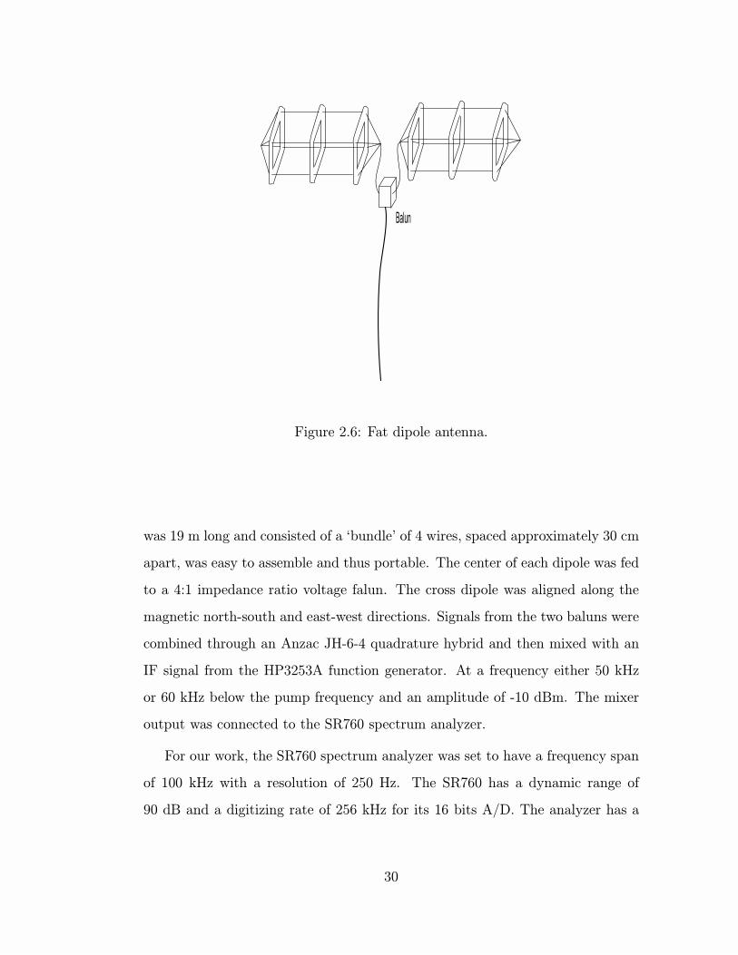
Balun
Figure 2.6: Fat dipole antenna.
was 19 m long and consisted of a ‘bundle’ of 4 wires, spaced approximately 30 cm
apart, was easy to assemble and thus portable. The center of each dipole was fed
to a 4:1 impedance ratio voltage falun. The cross dipole was aligned along the
magnetic north-south and east-west directions. Signals from the two baluns were
combined through an Anzac JH-6-4 quadrature hybrid and then mixed with an
IF signal from the HP3253A function generator. At a frequency either 50 kHz
or 60 kHz below the pump frequency and an amplitude of -10 dBm. The mixer
output was connected to the SR760 spectrum analyzer.
For our work, the SR760 spectrum analyzer was set to have a frequency span
of 100 kHz with a resolution of 250 Hz. The SR760 has a dynamic range of
90 dB and a digitizing rate of 256 kHz for its 16 bits A/D. The analyzer has a
30

built-in digital filter which filters and heterodynes the input in real time. The
SR760 offers four types of windowing functions. The Hanning window which is
the most commonly used window with amplitude variation of about 1.5 dB was
used throughout the project. The SEE spectra shown in the following chapters
are averages over 10 spectra with equal weighting in RMS to reduce fluctuations.
The SR760 was automated by a personal computer via GPIB. The processed data
was saved in the same computer.
2.2.3 Background Diagnostics
An ionosonde is a basic device used to measure the ionospheric electron density
distribution. A series of short pulses are transmitted upward to the ionosphere,
and then reflected from a layer whose local plasma frequency, ωp = (4πnee2/me)
1/2,
equals the incident wave frequency. The reflected pulse is recorded by a receiver
after a time delay equal to the total time of flight of the pulse, t. Giving the
pulse propagation at the speed of light, the virtual height, h0, can be obtained by
h0(f) = 1/2ct. Since the pulse is traveling in a plasma media, the speed of the
pulse is smaller than the speed of light. The value of the virtual height obtained
from the above equation is thus greater than the true height. A plot of the virtual
heights versus the corresponding frequencies is called an ionogram [49].
A vertical-incidence ionosonde, the Lowell Digital Ionospheric Sounding Sys-
tem (DISS), operated by the Air Force Space Forecast Center at Sheep Creek,
about 50 km west of HIPAS is available through a 1200/2400 baud modem con-
nection. It has a fixed probing time interval and frequency range, which provide
the general information on the density profile and the peak frequencies of the
ionospheric F1, F2, and E layers every 30 min. Another digital sounder, the
Lowell Digisonde model DPS-4, located at the HAARP facility, is accessible via
31

internet connection. The ionogram at the HAARP facility is updated every
15 min.
A Stanford Research Institute (SRI) digital ionosonde located at the NOAA
facility can be accessed and initialized through an internet connection. When
performing experiments at the HIPAS facility, the SRI ionosonde is set to sound
every 10 minutes to provide the ionospheric background condition at the receiving
site.
The critical frequencies of the ionospheric E and F layers are influenced by
the solar activities. When sunspots appear on the surface of the sun, strong
magnetic fields may be detected on earth. During a magnetic disturbance, ad-
ditional currents circulate in the ionosphere, especially at high latitudes, and
concentrate along the auroral field lines. Enhanced ionization in the ionosphere
causes stronger absorption in the E and D-regions. Both sunspots and solar flares
can greatly enhance ionospheric ionization [16]. Hence, both magnetic and solar
information is needed to predict the ionospheric conditions and to determine the
parameters in the experiments.
A magnetometer is an instrument for measuring the strength and direction of
magnetic fields on or near the Earth surface and in space. Using magnetometer
data, one can track the current state of the geomagnetic conditions including the
magnetic fluctuations due to auroral substorms and magnetospheric storms. A
riometer is a device using cosmic radio noise to measure ionospheric absorption.
This cosmic noise absorption has a sidereal variation from the changes in the
ionization and the condition of the upper atmosphere. Thus by monitoring the
background cosmic noise intensity on the ground, we can observe disturbances in
the ionosphere, which often reflect auroral events at higher latitudes. The mag-
netometer and riometer data are collected at both the High Latitude Monitoring
32

Station (HLMS) at Elmendorf Air Force base near Anchorage and at the United
States Geological Survey (USGS) College station as a part of the Space Environ-
ment Laboratory Data Acquisition and Display System (SELDADS) database.
The daily summaries of ionosphere and solar geophysical activities are avail-
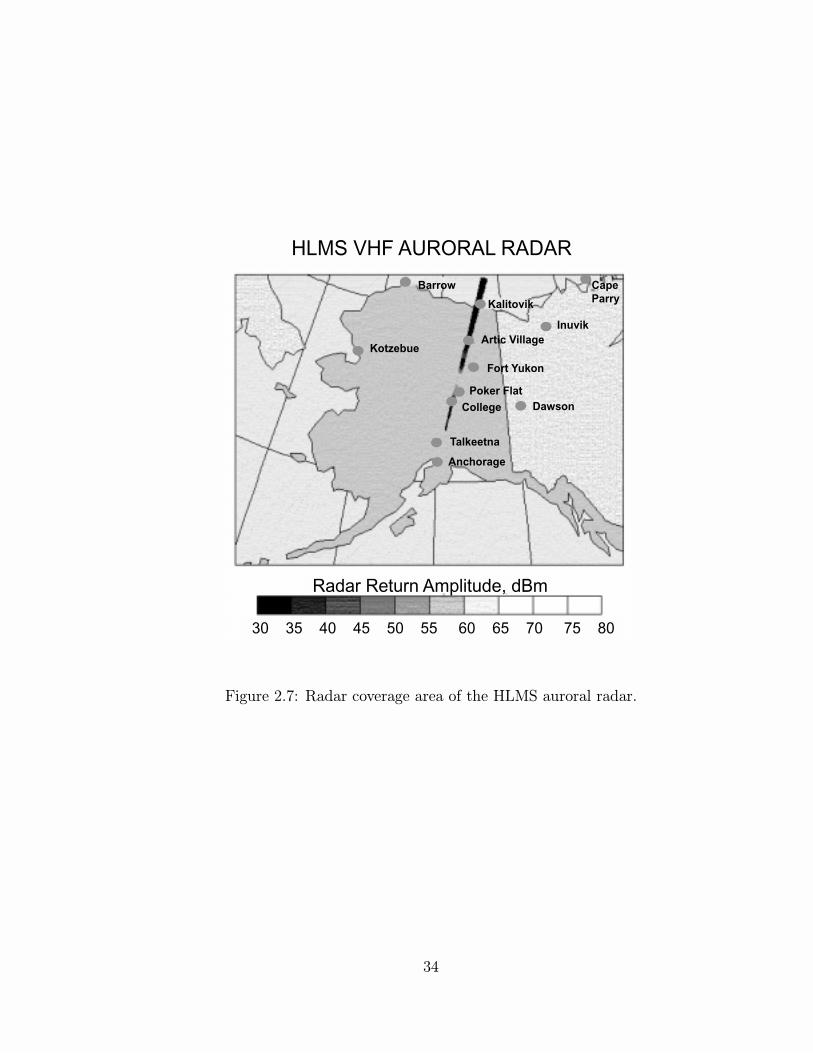
able on the internet (http://www.sec.noaa.gov/forecast.html). In addition, the
HLMS has a 50 MHz single beam radar that measures reflections from the auro-
ral structures in the E-region. It covers the distance from the Anchorage station
to approximately 100 miles north of HIPAS, ∼ 1200 km from the radar (Figure
2.7) .
The Super Dual Auroral Radar Network (SuperDARN) is an international col-
laborative program for scientific investigation of the upper atmosphere, ionosphere,
and magnetosphere. It is a network of high-frequency radars for studying the
Earth’s ionosphere. The SuperDARN consists of HF radars in the northern and
southern hemispheres. Three radars within this network observe the Alaska sec-
tor, Kodiak and King Salmon in Alaska, and Prince George in British Columbia.
The HAARP facility is centered in the Kodiak field of view at about 650 km
range. Each radar’s azimuthal scan is done in 16 sequential beams within 1
to 2 minutes. There are several scan modes for different temporal and spatial
resolutions. The primary product of the radars is line-of-sight plasma drift ve-
locity in the F-region. Combining all the velocity data from the entire northern
hemisphere network produces convection maps. The SuperDarn radars can also
determine the evolution of density irregularities generated by the HF heating in
the F-region.
33
HLMS VHF AURORAL RADAR
Radar Return Amplitude, dBm
30 35 40 45 50 55 60 65 70 75 80
CapeParry
Barrow
Artic Village
Fort Yukon
Inuvik
Kotzebue
Kalitovik
DawsonPoker Flat
College
Talkeetna
Anchorage
Figure 2.7: Radar coverage area of the HLMS auroral radar.
34

2.3 Conditions for the Experiment
The effect of matching at the peak frequency in the F layer is optimized under
quiet ionospheric conditions. These quiet conditions allow an unambiguous deter-
mination of the peak ionospheric plasma frequency foF2, a better determination
of the time window for the matching conditions, and reproducible experiments.
Normal absorption in the collisional D-region (70 — 90 km) is a prerequisite to
efficient coupling to the higher altitude. An ionosonde records the range of fre-
quency for observable return pulses and thereby determines the absorption in
the ionosphere. As a collisional absorption is inversely proportional to the HF
frequency, clear echo returns at low frequencies indicate low absorption and no
field-aligned precipitation. Magnetometer readings also help determine the con-
ditions in the ionosphere. A magnetic fluctuation of more than 300 nT implies a
very absorptive condition whereas a fluctuation of 100 to 200 nT suggests a high
electron density in the E-layer. The latter will cause an EM wave reflection at a
lower altitude. Thus, a minimal magnetic fluctuation is preferred for coupling the
EM wave to the F-layer. The process of ultraviolet (UV) ionization and molecular
recombination changes the ionospheric density profile. As a result, the electron
density is higher and more variant during daytime and in summer at high lati-
tude. For these reasons, the matching experiments are conducted between late
September and early April either in the morning or late in the afternoon.
35

CHAPTER 3
Reflected EM Wave under Matching Condition
This Chapter will present the experimental results on the density profile modi-
fications under the matching condition or when the heater frequency is equal to
the peak ionospheric plasma frequency, foF2 at the HIPAS facility.
3.1 Spreading of the Ionosonde Echo Returns
3.1.1 Setup of the Dynasonde
A joint campaign to measure the ionospheric modification was conducted in the
Fall of 1992, with the Utah State University (USU) Dynasonde group. The
ionosphere was modified using the HIPAS heater at a frequency of 2.85 MHz. The
digital USU Dynasonde was deployed at the NOAA facility during the campaign.
The receiving antenna array of the Utah Dynasonde had an L-shape with a cross
dipole at the corner as is shown in Figure 3.1. The reference point “O” was at
the center of the cross dipole pair. Each dipole was aligned along a side of the
“L” in the north-south and east-west directions. This set up was an improved
configuration by which the Dynasonde data could be processed with minimal
phase aliasing [92] . The Dynasonde transmitter was located approximately
200 m away from the receiver. The dynasonde used a TMS32010 DSP processor
and an echo detection scheme to eliminate interference and atmospheric noise
36

S
W E
O
N
D
D
Figure 3.1: The USU dynasonde receiving antenna array configuration. D is
typically 30 meters.
from the ionogram. The Dynasonde transmitted a group of four pulses at each of
the specified frequencies. Within the group, a small frequency increment of 8 kHz
was used for additional group height accuracy and tests of pulse dispersion. The
reflected echoes were received by the two dipole antennas for each pulse. A total
of eight echoes were received from one pulse set. The built-in software program
then converted these eight echoes into the echolocation, wave polarization, and
Doppler shift. More details on the Dynasonde can be found in the paper [92, 19,
18, 107, 108].
3.1.2 Experimental Results
During the Fall 92 campaign, the USU Dynasonde transmitted every three to six
minutes. Figures 3.2 and 3.3 show the Dynasonde results observed on October
37

11.
52
2.5
33.
54
4.5
50
100
200
300
400
500
600
700
800
Fre
quen
cy, M
Hz
Virtual Height, km
Uta
h D
ynas
onde
Oct
. 03,
199
2 05
:01
UT
Gil
mor
e C
reek
, AK
500
050
0
600
400
2000
200
400
600
EW
, km
NS, km
500
050
00
200
400
600
800
EW
, km
Virtual Ht., km50
00
500
0
200
400
600
800
NS
, km
Virtual Ht., km
2.2
2.4
2.65
2.9
3.15
3.4
Fre
quen
cy, M
Hz
X-m
ode
O-m
ode
Figure 3.2: Ionogram obtained on October 3, 1992 at 05:01 UT (before matching)
by the Utah Dynasonde. (Top panel) The ionogram shows a smooth F-layer
return at a peak frequency 3.5 MHz. The solid line indicates the pump frequency.
(Bottom panel) Skymaps show the scattering pattern of the O wave echo return.
Geomagnetic coordinate is used.
38
11.
52
2.5
33.
54
4.5
50
100
200
300
400
500
600
700
800
Fre
quen
cy, M
Hz
Virtual Height, kmUta
h D
ynas
onde
Oct
. 03,
199
2 05
:43
UT
Gil
mor
e C
reek
, AK
500
050
0
600
400
2000
200
400
600
EW
, km
NS, km
500
050
0
0
200
400
600
800
EW
, km
Virtual Ht., km50
00
500
0
200
400
600
800
NS
, km
Virtual Ht., km
2.2
2.4
2.65
2.9
3.15
3.4
Fre
quen
cy, M
Hz
X-m
ode
O-m
ode
Figure 3.3: Ionogram taken at 05:43 UT when the pump frequency matched the
foF2 at 2.85 MHz. (Top panel) The ionogram shows a spreading of the echoes
with a frequency span of approximately 0.8 MHz and the spatial disturbance
extends over a distance of 250 km. The solid line indicates the pump frequency.
(Bottom panel) Skymap during matching shows the O wave echoes spread more
towards the northeast direction and are closely aligned with the magnetic field
lines. Geomagnetic coordinate is used.
39

3, 1992. The HIPAS pump frequency was within the foF2 range, 2.75 — 2.95 MHz
(or 2.85 ± 0.1 MHz), from 0532 to 0558 Universal Time (UT). The heater causeda sudden increase in the signal to signal ratio at a frequency around 2.85 MHz.
Hence, the echo recognition process rejected all the data around 2.85 MHz and
leaves a gap in the O wave trace of the ionogram.
The USU ionograms showed clear non-spread echo returns from the F layer
before the heater frequency matched foF2 (Figure 3.2 top panel). As foF2 de-
creased towards the pump frequency at 2.85 MHz, the ionograms showed apparent
spreading around 2.85 MHz (Figure 3.3 top panel). The spread of the echoes
extended over a broad frequency range and a large spatial extent. The spread
had a frequency span of approximately 0.8 MHz, and the disturbance appeared
to extend over a distance of 250 km. The affected region corresponded to an
absolute density change of ∆n=4.8x102 cm−3 in the density profile.
The skymaps in Figure 3.2 and 3.3 display the O wave echo scatter locations
in the ionosphere before and during the matching, respectively. The (0,0) coordi-
nate refers to the zenith at NOAA using the geomagnetic coordinate system. The
(x,y) coordinates correspond to the virtual reflection location of the echo derived
from the angles of arrival. During the period of matching, the echoes spreaded
more towards the northeast direction and were closely aligned with the magnetic
field lines. This indicates that large-scale, field-aligned density striations are cre-
ated, giving rise to enhanced scattering of HF waves over an extended frequency
range.
3.1.3 Discussions
During the matching conditions, ionosonde echoes spreads more towards the
northeast direction, i.e., towards the geomagnetic pole (the magnetic declina-
40

tion at HIPAS is ∼ 26◦). As shown in Figure 3.4 , the O-mode shape spot is
asymmetric, leaning towards the northeast due to ray bending near the reflection
layer. Near the matching conditions, the resonance layer can extend as far as
60 km. Thus the strongest heating should result in an extended region northeast
of HIPAS where most of the echo locations are observed. The echo locations also
appear to align more or less along the magnetic field (Figure 3.3 bottom panel).
This is consistent with the model in which large spread of ionosonde echo returns
can be attributed to anomalous and multiple scattering of the echoes by FAS,
first initiated near the reflection region and then extended to align along the field
[26]. During the matching condition, only spreads at lower heights are observed.
Fewer data points are recorded in the matching case (Figure 3.3 bottom panel) in
comparison to the overdense case (Figure 3.2 bottom panel) since the ionosphere
is transparent to EM waves at frequencies greater than foF2. As foF2 decreases,
less echo returns are recorded on the ground within the same sounding frequency
range.
In conclusion, the USU ionograms show significant density perturbation dur-
ing the critical frequency match. Large density perturbation indicates the collapse
of caviton into smaller ones. The amount of turbulence can be estimated from the
variation in the wavenumber distribution. Individual caviton cannot be resolved
using an ionosonde alone, more diagnostics need to be introduced in the future.
3.2 Comparison Between X- and O-Mode Heating
X- and O-mode heating has been conducted several times. Every attempt was
made to ensure that the experiments were conducted under quiescent and repro-
ducible ionospheric conditions. Nevertheless, conditions did vary, and the data
presented here were recorded under different ionospheric conditions ranging from
41

B
ResonanceLayer
E
200 km
n(h)
1.4 x 10 /cm5 3
100 km
O mode
Phased ArrayMN
75 km
Figure 3.4: The ray paths computed from a cold-plasma theory. The Earth’s
magnetic field makes an angle of 13◦ with the density gradient at HIPAS.
42

being quiet to moderate magnetic activity. Experiments were usually performed
late in the afternoon or during the evening. During these periods of time, the
peak frequency in the F layer decreased from a value well above to below the
HIPAS operating frequency at 2.85 MHz or 4.53 MHz. Continuous wave (CW)
was used with continuous switching between O- and X-mode. The reflected sig-
nals from the pump were monitored using the HF narrow band receiver at the
NOAA facility.
3.2.1 Experimental Results
Figures 3.5 to 3.10 show the comparison between X- and O-mode CW heating
at 2.85 and 4.53 MHz. The ionospheric conditions were similar on these two days
with no presence of any E layer throughout the experiments.
A difference of 3 — 6 dB in the reflected amplitude is observed between X-
and O-mode heating until near the matching condition. Near the matching con-
dition, the signal strength of the O-mode skywave return decreases dramatically
so that the difference between the two modes becomes 10 — 15 dB (Figures 3.5
and 3.6). This appears to be a rather robust and reproducible phenomenon
under the matching condition for O-mode heating and indicates an anomalous
or enhanced absorption of the pump wave. Long density scale length, a large
interaction region, efficient mode conversion, and long interaction time (due to
slow convective loss as a result of long scale length) of the converted ES waves
all contribute to this effect and will be discussed in more details later.
The Doppler frequency shifts of the skywave return also show a significant
difference between X- and O-mode heating. Factoring the effects of statistical
noise and background fluctuations of the ionosphere, a net positive frequency
shift is observed from the O-mode heating and a smaller negative shift from
43

03:00 03:15 03:30 03:45 04:00 04:15 04:30 04:45 05:00-60
-50
-40
-30
-20
-10March 9,95 03:00-05:00 UT at 4.53 MHz
O mode X mode O mode average X mode average
Peak
Am
plit
ude o
f R
efle
cted W
ave
(dB
)
UT Time
Possible Matching Period
Figure 3.5: Data obtained on March 9, 1995 showing the amplitude of the re-
flected wave and the interpolated density profile generated from the DISS during
the experiments. The pump frequency was set at 2.85 MHz.
44

05:30 05:45 06:00 06:15 06:30 06:45 07:00 07:15 07:30 07:45 08:00
-50
-40
-30
-20
-10
O mode X mode O mode average X mode average
Pea
k A
mpl
itude
of R
efle
cted
Wav
e (d
B)
UT Time
March 22, 95 05:30-08:00 UT at 2.85 MHz
Possible Matching Period
Figure 3.6: Data obtained on March 22, 1995 showing the amplitude of the
reflected wave and the interpolated density profile generated from the DISS during
the experiments. Ionograms were taken only before and after possible matching
condition. The pump frequency was set at 4.53 MHz.
45

the X-mode heating. Figure 3.7 illustrates how frequency shifts become more
significant when the heater frequency is close to foF2. Since Doppler shifts of HF
waves in general indicate motion of the reflecting layers or density changes along
the ray path, the results appear to indicate that X- and O-mode heating produce
opposite layer motions or density changes. It should be emphasized that the ray
paths for the X- and O-modes are very distinct and quite far apart laterally for
high latitude launch as is the case at HIPAS and that the X-mode cutoff occurs at
a much lower height than that of the O-mode [8]. These observations have also
been reported [95, 96, 3, 4] at other HF heating facilities under non-matching
condition.
In addition, a spectral analysis of the skywave return shows dramatic broad-
ening in the skywave spectra during the matching condition. Figure 3.8, 3.9
and 3.10 show different degrees of broadening widths in the frequency spectra
during the matching period. An increase of more than 15 Hz in halfwidth (∆f )
was recorded on February 17 and September 20, 1995 (Figures 3.8 and 3.9) and
4 — 10 Hz on March 9 (Figure 3.10). The halfwidth of the frequency spectrum
is defined here as the full width at half maximum (FWHM), or the difference be-
tween each of the two frequencies at which the amplitude is equal to half the peak
amplitude (in dB) above the noise level. This dramatic increase in the halfwidth
of the spectrum during the matching condition indicates anomalous scattering
of the pump wave with enhanced low frequency fluctuations, parametric decay,
and mode coupling processes. As mentioned earlier, this is facilitated by the
large interaction region of enhanced ES wave turbulence. Again, this frequency
broadening phenomenon appears to be quite robust near the matching condition.
46
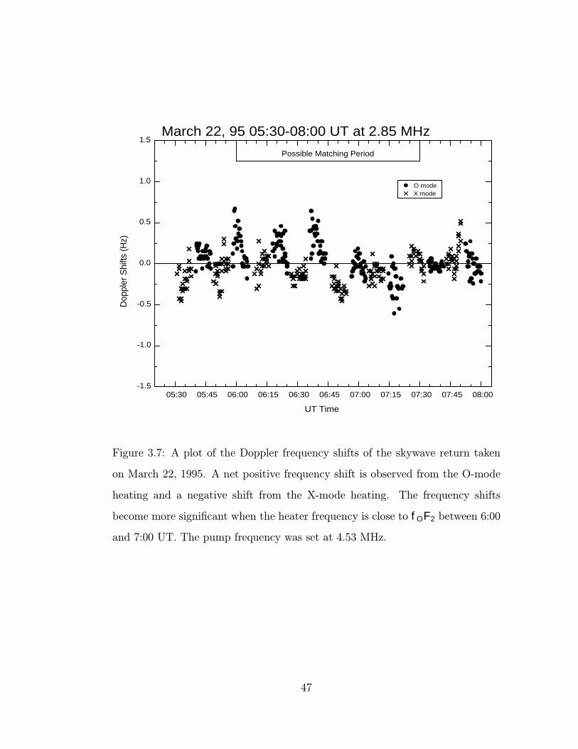
05:30 05:45 06:00 06:15 06:30 06:45 07:00 07:15 07:30 07:45 08:00-1.5
-1.0
-0.5
0.0
0.5
1.0
1.5March 22, 95 05:30-08:00 UT at 2.85 MHz
Possible Matching Period
O modeX mode
Dop
pler
Shi
fts (
Hz)
UT Time
Figure 3.7: A plot of the Doppler frequency shifts of the skywave return taken
on March 22, 1995. A net positive frequency shift is observed from the O-mode
heating and a negative shift from the X-mode heating. The frequency shifts
become more significant when the heater frequency is close to fOF2 between 6:00
and 7:00 UT. The pump frequency was set at 4.53 MHz.
47

05:30 05:45 06:00 06:15 06:300
5
10
15
20
25 O mode O mode average
February 17, 95 05:25-06:30 UT at 2.85 MHzH
alfw
idth
(Hz)
UT Time
Possible Matching Period
Figure 3.8: A plot of FWHM of the reflected pump signals as function of time
for the data taken on February 17, 1995. CW O-mode heating was used. The
solid line shows the average halfwidth for every five-minute interval. The pump
frequency was set at 2.85 MHz.
48

05:00 05:15 05:30 05:450
5
10
15
20
25
30
O mode O mode average
September 20, 95 05:00-05:50 at 2.85 MHz
Halfw
idth
(H
z)
UT Time
MatchingMatching
Figure 3.9: A plot of FWHM of the reflected pump signals as function of time
for the data taken on September 20, 1995. CW O-mode heating was used. The
solid line shows the average halfwidth for every five-minute interval. The pump
frequency was set at 2.85 MHz.
49

03:00 03:15 03:30 03:45 04:00 04:15 04:30 04:45 05:000
2
4
6
8
10
12
O mode X mode O mode average X mode average
March 9, 95 03:00-05:00 UT at 4.53 MHzH
alfw
idth
(H
z)
UT Time
Possible Matching Period
Figure 3.10: A plot of FWHM of the reflected pump signals as function of time
for the data taken on March 22, 1995. A halfwidth of 4—10 Hz was observed
when the heater frequency was close to foF2 between 03:45 and 04:45 UT. The
solid and dashed lines show the average for each O- and X-mode heating cycle,
respectively. The pump frequency was set at 4.53 MHz.
50

3.2.2 Discussions
F layer heating effects are consistently the strongest for O-mode heating based on
previous observations on HF heating [93, 15, 84, 46, 103]. For overdense heating
the amplitude of the pump wave can be strongly affected by D-region absorption,
difference in the reflection height, and F-region scattering of the EM waves into
the Langmuir waves from small scale FAS, i.e. anomalous absorption.
A powerful wave of either polarization is capable of causing a strong increase
in the D-region absorption [38, 24]. The steady amplitude from the X-mode
skywave return throughout the experiments (Figures 3.5 and 3.6) provides
conclusive evidence that the decrease in the O-mode skywave return signal when
near matching is caused by the D-region absorption. The nondeviative absorption
(ΓD) of an EM wave transversing the D-region depends on the frequency [101, 73]
ΓD ∝ (f ∓ fl)−2 (3.1)
where f is the EM wave frequency, and fl is the longitudinal component of the
electron gyrofrequency. The plus and minus signs correspond to the O- and X-
modes, respectively. From equation 3.1, the X-mode absorption is expected to
be larger than the O-mode absorption. However, our data show that the O-mode
skywave return signal is weaker than that of the X-mode and further proves that
the decrease in O-mode is not due to the D-region absorption.
We can also exclude the mechanism due to the different reflection heights for
O- and X-mode. An O-mode wave was reflected at a height between 250 and
300 km during the experiments conducted on March 9 and 22, 1995. Though an
X-mode wave reflects at a lower altitude than an O-mode wave, their difference
in the power density, assuming 1/r2 dependence is less than 5 dB. Our observed
values before matching lie within this range. However, this mechanism does not
51

explain the 10-15 dB difference in the amplitude observed during the period of
matching.
As mentioned earlier, large enhanced electric field, mode conversion, and lo-
cal heating near the reflection layer lead to profile modifications. Due to the
anisotropy in transport rates, the parallel rate is at least 3 orders of magnitude
larger than the perpendicular rate. As a result, density perturbations can elon-
gate to form FAS and further enhance the mode conversion process leading to
anomalous absorption of the pump EM wave. Once these striations are formed,
parametric instabilities can occur preferentially within. One such instability is
the decay or conversion of the pump EM wave to an UH wave. The electrostatic
UH wave has a short wavelength and can be trapped inside the striations. Thus
an efficient feedback process can result when the pump EM wave generates the
striations, which then cause conversion of EM wave to an UH wave, which in
turn steepens the striations that further enhance wave conversion and anomalous
absorption [21, 66, 67]. Clearly this is an efficient and highly nonlinear mecha-
nism for the absorption and damping of the pump wave. Anomalous absorption
effects have been reported during the O-mode heating of the F layer ionosphere.
A considerable diagnostic amplitude reduction of up to 10 dB during the O-
mode heating is observed, while the X-mode heating shows less than 1 dB change
[93, 15, 84]. However, such results were obtained under normal heating scenarios
without the matching condition. It remains to be seen theoretically whether the
efficiency of such a process can be further enhanced by the matching condition.
The difference in Doppler shifts for the X- and O-mode heating, as discussed
earlier, can probably be attributed to the difference in ray paths and cutoff height
for the two-modes. When the heater frequency matches foF2, the X-mode cutoff
height can be 50 km below that of the O-mode. Large Doppler shifts observed dur-
52

ing the matching condition indicate strongly induced layer motions and density
changes consistent with strong wave activities and turbulence in the extended
interaction region. The positive shift during the O-mode heating is consistent
with the elongation of the depleted density striation towards lower height. For
the observed Doppler shift values in the range of about 0.5 Hz (Figure 3.7), the
calculated Doppler velocity is about 125 m/s. This is equivalent to a plasma drift
from an ambipolar electric field of about 25 mV/m, a value frequently observed
at high latitudes. In comparison, thermal diffusion time for the sizes of the beam
spot and large interaction region is about 10 minutes, too slow to account for the
observed Doppler shifts.
The negative shift during the X-mode heating, can be explained by the up-
ward motion of the plasma at the X-mode reflection layer, back-filling the per-
turbed depleted region at higher heights created by the previous cycle of the
O-mode heating. The observation of opposite Doppler shifts for the two polar-
izations, is therefore consistent with the physical picture of plasma expulsion and
refilling during the nonlinear heating processes. As mentioned earlier, observa-
tions of both positive and negative Doppler shifts have been reported recently
[95, 96, 3, 4]. The positive Doppler shifts have been attributed to density in-
creases from either a reduction in recombination rates or to enhance ionization
from accelerated electrons during the HF heating. The negative shifts, on the
other hand, have been attributed to density depletions and striations caused by
intense ES wave intensity. In these experiments, test HF waves at multiple fre-
quencies were launched and their Doppler shifts were recorded during the O-mode
heating under non-matching conditions. In our work, only the Doppler shifts of
the HF pump waves were recorded. A multiple frequency HF Doppler diagnostic
is currently being tested at HIPAS.
53
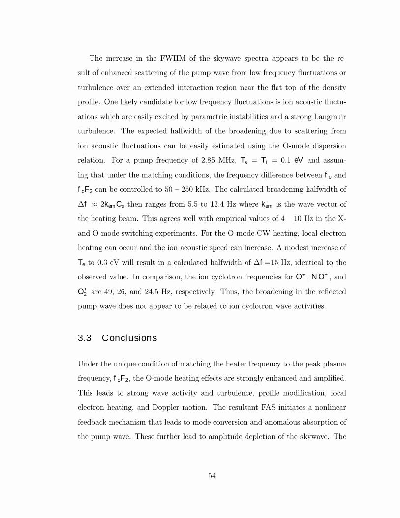
The increase in the FWHM of the skywave spectra appears to be the re-
sult of enhanced scattering of the pump wave from low frequency fluctuations or
turbulence over an extended interaction region near the flat top of the density
profile. One likely candidate for low frequency fluctuations is ion acoustic fluctu-
ations which are easily excited by parametric instabilities and a strong Langmuir
turbulence. The expected halfwidth of the broadening due to scattering from
ion acoustic fluctuations can be easily estimated using the O-mode dispersion
relation. For a pump frequency of 2.85 MHz, Te = Ti = 0.1 eV and assum-
ing that under the matching conditions, the frequency difference between fo and
foF2 can be controlled to 50 — 250 kHz. The calculated broadening halfwidth of
∆f ≈ 2kemCs then ranges from 5.5 to 12.4 Hz where kem is the wave vector of
the heating beam. This agrees well with empirical values of 4 — 10 Hz in the X-
and O-mode switching experiments. For the O-mode CW heating, local electron
heating can occur and the ion acoustic speed can increase. A modest increase of
Te to 0.3 eV will result in a calculated halfwidth of ∆f=15 Hz, identical to the
observed value. In comparison, the ion cyclotron frequencies for O+, NO+, and
O+2 are 49, 26, and 24.5 Hz, respectively. Thus, the broadening in the reflected
pump wave does not appear to be related to ion cyclotron wave activities.
3.3 Conclusions
Under the unique condition of matching the heater frequency to the peak plasma
frequency, foF2, the O-mode heating effects are strongly enhanced and amplified.
This leads to strong wave activity and turbulence, profile modification, local
electron heating, and Doppler motion. The resultant FAS initiates a nonlinear
feedback mechanism that leads to mode conversion and anomalous absorption of
the pump wave. These further lead to amplitude depletion of the skywave. The
54

pump wave and other EM waves (radiated by the ionosonde) are also strongly
scattered by the striations leading to large broadening in the reflected pump wave
and thus spread of the echo returns.
55

CHAPTER 4
Spectral Structure of SEE under Matching
Condition
This chapter presents the SEE results from both HIPAS and HAARP facilities,
obtained at both sunrise (when foF2 slowly builds up and passes the pump fre-
quency from below) and during sunset (when foF2 slowly decreases).
4.1 High Power Pumping
The SEE experiments were performed using the HIPAS and HAARP heating
facilities. The heater was turned on in full power for several minutes. The pump
frequency was at least 200 kHz from the nearest harmonic of the ionospheric
electron cyclotron frequency to minimize the gyroharmonic effects [57, 83].
4.1.1 Experimental Results
Under overdense pumping, the SEE sidebands are generally composed of a BC
and DM. They are excited within 3 s from the pump turn on after a cooling
period of 3 min or more, or a “cold start”. Anomalous absorption [15, 84, 31] is
commonly observed after the pump has been turned on for a few seconds. Figure
4.1 shows the temporal evolution of the reflected pump wave at 4.53 MHz and
the SEE signal at -10 kHz from fpump. After the high power pump is turned on
56

0 10 20 30 40 50 60 70 80-50
-40
-30
-20
-10A
mplit
ude, dB
V17 November, 1997 21:02:55 UT
0 10 20 30 40 50 60 70 80
-105
-100
-95
-90
-85
-80
Am
plit
ude, dB
V
Time, s
Time, s
Figure 4.1: Temporal evolution of the reflected pump wave at 4.53 MHz (top
panel) and the SEE signal at -10 kHz from fpump (bottom panel). A gradual
increase is observe in the bottom panel during the first 10 s. Data were taken at
cold start.
57

at t = 0 s, the reflected pump signal (top panel) drops from a level of -15 dB
to -25 dB after 10 s. This drop in the signal strength is generally attributed
to the anomalous absorption of the pump signal as a result of the formation of
striations. The SEE signal at -10 kHz (bottom panel) shows a gradual increase
in the signal strength within the first 10 s after the pump is turned on. These
two plots clearly show that the growth of SEE is correlated with the decline of
pump signal and the excitation of striations.
With the presence of preexisting striations, strong overshoot at the turn on
of the pump can be observed in the reflected pump signal and the SEE signal
at -10 kHz (Figure 4.2). This is in contrast to those observed during cold start
(Figure 4.1). The overshoot lasts for less than a second which is followed by a
quick drop with the signal level settling into the same range above noise level as
during cold start. Such overshoot can be easily reproduced; however, it is absent
when the pump frequency is at 6.8 MHz, 7.7 MHz, and 8.05 MHz, and this is
consistent with results reported in other facility [31].
A change in the SEE spectra is observed as foF2 becomes close to the pump
frequency. Figure 4.3 shows a sequence of spectra taken when HIPAS is transmit-
ted at fpump = 4.53 MHz as foF2 increased. The horizontal scale of the spectra is
the frequency offset from the pump. During the matching conditions, a distinct
and strong DM feature is excited on top of the BC backgrounds is shown in figure
4.3. When the pump frequency is above foF2, (Figure 4.3 (b) and (c)) the DM
feature becomes barely observable above the BC background . Moreover, the BC
has a signal strength ∼ 10 dB weaker and a few kilohertz narrower than that
observed during the matching condition. Figure 4.4 shows another set of spectra
taken at HAARP using a higher pump frequency, fpump = 5.9 MHz. Both the
BC and DM features are distinctively excited under the overdense conditions.
58

0 5 10 15 20 25 30 35 40-50
-40
-30
-20
-10
0A
mplit
ude, dB
V
Time, s
17 November, 1997 21:55:52 UT
0 5 10 15 20 25 30 35 40 -100
-90
-80
-70
-60
-50
Am
plit
ude, dB
V
Time, s
Figure 4.2: Temporal evolution of the reflected pump wave at 4.53 MHz (top
panel) and the SEE signal at -10 kHz from fpump. Strong overshoot is observed
immediately after turn-on. Data were taken during high power heating after
pre-heating the ionosphere.
59

40 20 0-100
-90
-80
-70
-60
-50
-40
-30
-20
Frequency, kHz
Am
plit
ud
e, d
B
foF2 ~ 4.5 MHz
40 20 0
foF2 ~ 4.9 MHz
40 20 0
foF2 ~ 5.4 MHz
17 November, 1997
-100
-90
-80
-70
-60
-50
-40
-30
-20
-100
-90
-80
-70
-60
-50
-40
-30
-20
(a) (b) (c)
DM
DM
Figure 4.3: Frequency spectra taken on November 17, 1997 at HIPAS with fpump
= 4.53 MHz under different values of foF2. The horizontal scale is the frequency
offset from 4.53 MHz.
60

60 40 20 0
-120
-110
-100
-90
-80
-70
-60
-50
-40
Am
plit
ude, dB
foF2 ~ 5.6 MHz
60 40 20 0
Frequency, kHz
foF2 ~ 5.8 MHz
60 40 20 0
foF2 ~ 6.1 MHz
DM
DM
DM
(a) (b) (c)
24 March, 2001
-120
-110
-100
-90
-80
-70
-60
-50
-40
-120
-110
-100
-90
-80
-70
-60
-50
-40
Figure 4.4: Frequency spectra taken on March 24, 2001 at HAARP with fpump
= 5.9 MHz under different values of foF2.
61

The BC, however, is again much stronger and wider when foF2 is near the pump
frequency.
We have continuously recorded the SEE spectra when foF2 was passing through
the pump frequency at 7.4 MHz from above (Figure 4.5). The BC clearly contin-
ues to decrease in signal strength, but the intensity of the DM feature remains
unchanged. Figure 4.6 shows spectra for foF2 a few 100 kHz below the pump
frequency at 4.56 MHz. The only emission observed under this condition is the
DM feature, as is also observed in Tromsø [58].
4.1.2 Discussion
During high power pumping near the matching conditions when foF2 decreased
from the overdense to matching conditions, the strength of the DM feature as
well as the width of the sidebands increase (Figure 4.3). The reason for this
behavior is unknown. It may simply be a decrease in the absorption of the pump
wave, such as a decrease in the excitation level of the Langmuir turbulence near
the pump reflection height, because of a decreasing swelling in the pump electric
field, as the background plasma density gradient decreases near matching. When
foF2 decreases slightly below the pump frequency the excitation of Langmuir
turbulence is suppressed by the absence of plasma resonance. As a result, the
reflected pump wave decreases in the signal strength. This makes it difficult
to estimate the influence on the excitation of the UH turbulence without more
detailed modeling.
The strong SEE features during the matching condition may be explained
by the increase in the interaction lengths in the more homogeneous background
plasma density profile. This is similar to what has been suggested for the inten-
sification of 630-nm airglow during matching [5].
62
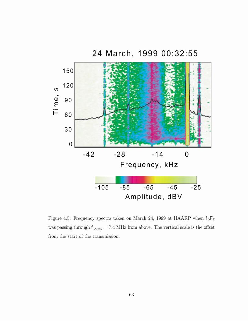
Tim
e,
s
Ampl i tude, dBV
150
120
90
60
30
0
-105 -85 -65 -45 -25
-42 -28 -14 0
24 March, 1999 00:32:55
Frequency, kHz
Interference
Figure 4.5: Frequency spectra taken on March 24, 1999 at HAARP when foF2
was passing through fpump = 7.4 MHz from above. The vertical scale is the offset
from the start of the transmission.
63

40
30
20
10
0
-30 -20 -10 0 10
-125 -105 -85 -65 -45
Ampl i tude, dBV
Frequency, kHz
Tim
e,
s14 March, 1999 03:24:56
Interference
Figure 4.6: Frequency spectra taken on March 14, 1997 at HIPAS when foF2 was
a few 100 kHz below fpump = 4.56 MHz.
64

As foF2 passed through the pump frequency from above, the BC eventually
decreased in strength without a corresponding decrease in the DM (Figure 4.5).
When foF2 was a few 100 kHz below the pump frequency, the only SEE fea-
ture observed was a weak DM (Figure 4.6). These experimental results seem
inconsistent with theoretical interpretations of the DM for trapped upper-hybrid
oscillations in striations [39, 68, 51] and the BC for freely propagating UH waves
[35, 78, 36]. In order to trap upper-hybrid oscillations a higher plasma density is
required than freely propagating waves at the same frequency. Given that the BC
depends on the electron gyroharmonics and the excitation of UH waves as is sug-
gested by its slow evolution on the thermal time scales after a cold start [56], the
experimental results suggest that the BC also depends on the trapping of upper-
hybrid oscillations. Excitation of trapped upper-hybrid oscillations leads to high
oscillation amplitudes. We therefore conjecture that the BC depends on escape
of the trapped oscillations by scattering of the initial trapped oscillations from
nearly perpendicular to the geomagnetic field toward smaller angles where they
can escape from the trapping density depletion. The wide spectrum of the BC can
then be generated by the oblique UH waves, by induced scattering of ions along
the lines previously suggested without considering initial trapping [35, 78, 36].
As foF2 decreases and passes through the pump frequency from above, electron
plasma waves exist at successively smaller angles to the geomagnetic field for the
successively lower foF2 because of linear dispersion. The excitation of oblique
waves will therefore cease before the excitation of perpendicular trapped oscil-
lations, and the BC would be suppressed before the DM, consistent with the
experimental results. The dependence of the DM on the interaction of upper and
lower-hybrid oscillations requires the oscillations to be highly perpendicular to
the geomagnetic field. In addition, the weak residual DM seen near the upper-
hybrid matching condition (Figure 4.6) may also have contributions from freely
65

propagating UH waves [109, 76].
Measurements on the anomalous absorption in future experiments are highly
recommended to compare the overdense and matching cases. Anomalous absorp-
tion is caused by the excitation of small scale density striations which, in turn,
is an aspect of the driven upper-hybrid turbulence [41]. To measure the anom-
alous absorption therefore gives an indication of the intensity of upper-hybrid
phenomena. However, more diagnostics will be necessary in future experiments
to include the measurement of the anomalous absorption.
4.2 The Effect of Preconditioning on Low Power Pumping
The effect of preconditioning was investigated by transmitting a sequence of low
power pulses alternating with high power pump pulses. By using this pump
sequence it was previously found that the DM could be excited at a low pump
power of ∼ 80 kW during the overdense conditions, if the ionosphere had been
preconditioned, in this case, with ∼ 20 MW effective radiated power [13]. These
experimental results agree well with theoretical predictions [39, 68, 69]. The DM
is excited via the decay of the trapped upper-hybrid oscillations in pre-formed
density depletion regions during the low power pulsing.
4.2.1 Experimental Procedure
A special heating sequence is used to perturb the ionosphere which is then probed
by a sequence of low power short duration transmissions (Figure 4.7). The cycle
starts with a sequence of low power test waves, T1, to ensure the ionosphere
is in the unperturbed state. It is followed by a 120 — 140 s high power CW
transmission, H1, to heat the ionosphere. The following T2 (H2) serves as the
66

0
0.09
40
Time, minute
ER
P, M
W
H1 H2
T1 T2 T3
Cooling
0 3 15 28 41
f
fdf
f+df
Time, second
0 1 2 3 4 5 6 7 8 9 10
Fre
qu
en
cy
H1
T2
H2
Figure 4.7: (a) Heating schemes used during the pre-conditioning experiments
and (b) detailed procedure for the low power heating sequence.
67

low (high) power probe in the pre-heated region. H2, meanwhile, further modifies
the ionosphere for another 120 — 140 s. The last sequence T3, is used to diagnose
the ionosphere after prolonged heating (H1 and H2). The cycle ends with a
cooling period of 200 — 230 s to allow the ionosphere to return to its unperturbed
state. A 3 sec off period is added in between each sequence for the transmitter
frequency change and as a time marker for the data acquisition. Each full cycle
is 10 minutes in duration.
Three different test frequencies are transmitted consecutively in each of the
40 s low power (ERP of ∼ 0.1 MW) transmissions (T1, T2, and T3) (Figure
4.7b). The test frequencies are set in the order of fpump + δf , fpump − δf , andfpump where δf ≤ 30 kHz. As soon as the test frequency becomes greater thanfoF2, the corresponding test wave will pass through the ionosphere and only a
small portion of its power will be reflected back. As a result, the low power
transmissions determine the matching period and at the same time probe the
heated region.
4.2.2 Experimental Results
The following results were obtained during the low power pumping using the
aforementioned heating scheme. No SEE was observed during the first low power
sequence (T1) under both the overdense and near matching conditions. This
indicates an unperturbed ionosphere state. However, once the ionosphere was
preconditioned by the high power sequence (H1 and H2), the SEE features were
excited during the following T2 and T3 low power sequence.
Figures 4.8 and 4.9 show the spectrograms of the T2 sequence data taken
on November 17, 1997 using the HIPAS facility with fpump = 4.53 MHz and
δf = 25 kHz. The horizontal axis is the frequency offset from 4.53 MHz and
68

25 0 25
3
13
23
33
43
Frequency, kHz
Tim
e,
sec
17 November, 1997 19:45:56
91 71 51 31
Amplitude, dBV
Figure 4.8: Frequency spectra taken on November 17, 1997 at HIPAS during the
T2 sequence under matching condition. The axes are the frequency offset from
4.53 MHz and the time offset from the time the H1 sequence is off.
69
-25 0 25
3
13
23
33
43
Frequency, MHz
Tim
e,
sec
17 November, 1997 20:15:54
-91 -71 -51 -31
Amplitude, dBV
Figure 4.9: Frequency spectra taken on November 17, 1997 at HIPAS during the
T2 sequence under overdense condition. The axes are the frequency offset from
4.53 MHz and the time offset from the time the H1 sequence is off.
70

the vertical, the time offset from the time when the high power pumping (H1)
was turned off. Under matching conditions (Figure 4.8), the sidebands of all
three test waves were at least 10 kHz wider. The DM feature was distinctively
observable with an amplitude of a few dB above the continuum.
Under both the matching (Figure 4.8) and overdense conditions (Figure 4.9),
the continuum developed during the first test wave transmission at fpump + δf .
At the second test wave (fpump−δf) transmission, the sideband was already fullydeveloped at the turn on of the transmitter in both conditions. The continuum
extends to a frequency range of ∼ 18 kHz when it was fully developed during
the overdense condition, but more than 25 kHz during the matching condition.
This is referred to as low power continuum (LPC). Since the receiving system had
only 100 kHz bandwidth, it was not possible to record the full SEE spectra when
transmitting the second test wave. At the last test wave (fpump) transmission, the
overdense continuum had a frequency extent of ∼ 18 kHz with a signal strengthof a few dB above the noise level and was weaker than those observed during
the previous second test wave transmission. The continuum excited under the
matching condition was much wider and stronger with a frequency extent of
∼ 40 kHz and a signal 10—15 dB stronger than those excited under the overdensecondition.
During the T2 and T3 low power transmissions, the DM feature was imme-
diately observed under the matching condition and the continuum feature took
∼ 10 sec to fully developed. The temporal evolution of the SEE signal at -10 kHzwith respect to each test frequency as shown in (Figure 4.10) suggested that there
was a growth period of ∼ 6 sec in both conditions. Data was taken on November17, 1997 using the HIPAS facility with fpump = 4.53 MHz and δf = 25 kHz.
When the maximum intensity level was reached, the signal became steady and
71

-5
0
5
10
15
20
25
30November, 17, 1997
4.555 MHz4.505 MHz4.530 MHz(a)
5 10 15 20 25 30 35 -5
0
5
10
15
20
25
30
Time after H1 off, sec
(b)
Am
plit
ud
e,d
B
Figure 4.10: Temporal variation in intensity of SEE signal at 10 kHz below
each test frequency during T2 transmission at (a) matching and (b) overdense
condition. The signal is more steady and stronger when matched and gradually
decreased to noise level when overdense. The average noise level is set to 0 dB.
72

independent of the transmitting frequency during matching, whereas it became
unstable and decreased gradually to noise level under the overdense condition.
From the difference in steadiness of the signal, we conclude that heating effects
are enhanced and sustained during a matching condition. Similar results were
a l so ob ser ve d du r i ng T3 tra ns miss io n.
Figure 4.11 shows spectra taken within 0.5 s after the turn on of the T2
sequence with the test frequency at fpump + δf . A distinct DM peak ∼ 5 dB
above a narrow LPC was immediately excited near the matching condition (solid
line). During the overdense heating, only a very narrow continuum of width
∼ 10 kHz was excited (dotted line), whose signal strength was 10 dB weaker
than that excited under the matching condition. However, the amplitude of the
reflected pump wave was also 10 dB stronger in the overdense case.
Figures 4.12, 4.13, and 4.14 show another set of T2 data taken at the HAARP
facility on March 24, 2001 with a higher pump frequency, fpump = 5.9 MHz.
Only the first 32 s of the T2 sequence was recorded. After the ionosphere was
preconditioned for 120 s, 18 s less than the previous case, the low power sequence
(T2) was turned on after a 5 s off period. Furthermore, only one test frequency
(fpump+δf) was used throughout the T2 sequence. The spectra were taken when
foF2 was about 6.1 MHz, 6 MHz, and 5.8 MHz from the panel top to bottom,
respectively. As foF2 approached the test frequency (Figure 4.13), the SEE
sidebands appeared for a longer period of time while the signal strength of the
DM feature was stronger than those observed during overdense condition. When
foF2 was slightly below the test frequency (Figure 4.14), the DM feature became
distinct on top of a narrow LPC that continued to exist throughout the recorded
32 s.
Previous experiments have observed large scale modifications of the ionospheric
73

-50 -40 -30 -20 -10 0 10 20-110
-100
-90
-80
-70
-60
-50
-40
-30
-20
Spectra taken at the turn on of the 4.555 MHz transmission
Frequency, kHz
Am
plitu
de
Near Matching
Overdense
DMInterference
Figure 4.11: Frequency spectra taken at 0.5 s after the turn on of the T2 sequence
at 4.555 MHz under the matching (solid line) and overdense condition (dotted
line).
74

40 -30 -20 -10 0
5
15
25
35
Frequency, kHz
Tim
e,
sec
25 Mar, 2001 02:42:42
-124 -114 -104 -94Amplitude, dBV
Figure 4.12: Frequency spectra taken on March 24, 2001 at HAARP during the
T2 sequence at 5.93 MHz. Data was taken when foF2 was about 6.1 MHz under
the overdense condition.
75

40 -30 -20 -10 0
5
15
25
35
Frequency, kHz
Tim
e, se
c25 Mar, 2001 02:02:48
-124 -114 -104 -94
Amplitude, dBV
Figure 4.13: Frequency spectra taken on March 24, 2001 at HAARP during the
T2 sequence at 5.93 MHz. Data was taken when foF2 was about 6 MHz near the
matching condition.
76

40 -30 -20 -10 0 5
15
25
35
Frequency, kHz
Tim
e,
sec
25 Mar, 2001 01:52:49
-124 -114 -104 -94
Amplitude, dBV
Figure 4.14: Frequency spectra taken on March 24, 2001 at HAARP during the
T2 sequence at 5.93 MHz. Data was taken when foF2 was about 5.8 MHz under
the slightly underdense condition.
77

density profile when the pump frequency was near the critical frequency [34, 103].
However, the ionograms from our experiments do not indicate any large scale per-
turbations in the density profile.
4.2.3 Discussion
The experimental results from preconditioning with low power pumping for the
matching and overdense conditions are similar to those from high power pumping.
The SEE is stronger under the matching conditions (Figure 4.8 and 4.9). This
again can be attributed to decreased absorption by suppression of the Langmuir
turbulence excitation and/or increased pump—plasma interaction lengths in the
more homogeneous background plasma near the peak of the ionospheric density
profile. The slow growth of the SEE in the first low power pulse within T2 after
the preconditioning appears similar to the increase in the SEE intensity during the
low duty cycle pumping with short pulses (so called diagnostic SEE) followed by
the high duty cycle pumping. This has also been observed in experiments at the
Sura facility in Russia [27] and in computer simulations [78, 36]. The increase
in SEE intensity is attributed to the decrease in the anomalous absorption of
the pump and the decay of the short scale striations after the high duty cycle
pumping (i.e., the preconditioning) is turned off [36]. The following decrease in
intensity in the last pulse during T2, is due to the longer decay of larger scale
striations that are sources for the SEE. Consequently, the source of the SEE
is not associated with only the smallest scale irregularities. Furthermore, the
present low power spectra (T2) show both a DM and LPC. The experimental
results reported by [58] on the low power transmission of approximately 86 kW
ERP after 30-s preconditioning at 270 MW ERP only have observed continuum
feature and not a DM. The low power continuum appears to have an even lower
78

threshold than the DM from the low power pumping after preconditioning.
4.3 Conclusion
In this chapter, SEE spectra from the overdense to underdense conditions are
compared. The strength of the DM and the width of the BC and LPC increase
when the pump frequency is near the matching condition for both the high and
low pump powers after preconditioning. These may be caused by the decrease
in absorption of the pump wave and/or the increase in the interaction lengths
near the peak of the profile. To further understand the mechanisms of these
changes, we need to include measurements on the anomalous absorption in future
experiments.
The experimental results of preconditioning on the low power pumping are
similar to the diagnostic SEE observed by [27]. According to Frolov [27] and
computer simulations [78, 36], the increase in the SEE intensity observed during
the beginning of the low power pumping sequence (T2 and T3) is a result of
the short scale striations decay after the high duty cycle pumping. The decrease
in the SEE intensity later in the sequence is attributed to the decay of larger
scale striations also on a longer time scale. However, no actual measurement of
the irregularities are taken together with the presented data, but this should be
included in future experiments when an incoherent backscatter radar is installed
in Alaska.
79
CHAPTER 5
Spectral Structure of SEE at 2fce
This chapter presents observations of SEE excited at a pump frequency near the
second harmonics of the ionospheric electron cyclotron frequency, i.e. fpump ≈ 2fce,
in the ordinary mode. A new type of the SEE feature is observed. The new fea-
ture, referred to as the “narrow symmetrical structure” (NSS), consists of two
spectral peaks, symmetrically located around the pump frequency fpump. The
frequency offset of the peaks from fpump are between 15 and 30 kHz.
5.0.1 Experimental Results
The experimental results were obtained in nighttime in February and March, 2003
at the HIPAS heating facility. Three different heating schedules were introduced
to investigate the SEE spectral structure excited near 2fce. Preconditioning ex-
periments used a similar schedule to that described in the previous chapter for
only one frequency in the low power sequence (T1, T2, and T3). The high power
sequence used 2.85 MHz, and the low power sequence, 2.875 MHz. The second
schedule was stepping the pump frequency between 2.84 MHz and 2.88 MHz in
steps of 1 kHz every 10 sec. The last schedule was power stepping experiment
conducted immediately after the frequency stepping schedule. The total output
power was stepped by means of increasing or decreasing the number of trans-
mitters every 25 sec and at a frequency determined by the frequency stepping
80

experiment.
Figure 5.1 shows the spectrogram from using the preconditioning schedule.
No SEE spectral structure is observed during any of the high power heating
at 2.85 MHz. However, both upper and lower sidebands are excited during the
100 kW low power heating at 2.875 MHz, even before preconditioning. By varying
the output power of the low power sequence, no sidebands are excited at all with
an output power of 50 kW (Figure 5.2). Lower sidebands are excited only after
preconditioning at output power of 75 kW (Figure 5.3). The observed sidebands,
however, are neither the DM, BC nor the BUM. They are symmetric sidebands
with multiple peaks and stronger in the lower sidebands at 100 kW power. The
sidebands peaks are ∼ 15 kHz apart, ∼ 5 kHz wide and 5 dB above noise. Thelower sidebands have intensity stronger than the upper sidebands. Only a single
lower sideband peak at ∼ 22 kHz below the pump is observed at 75 kW power
level.
The narrow symmetric sideband peaks (NSS) are excited within a narrow
range from the pump frequencies (Figure 5.4). These peaks are within 15-30 kHz
from fpump. The NSS are also excited at a different range of pump frequencies
(Figure 5.5).
The results from the power stepping measurement suggest a threshold level
about 56 kW in order to excite the SEE. Figure 5.6 shows the pump frequency
at 2.88 MHz, while the NSS is excited 28 kHz from it. The lower sideband is
more intense and has a wider bandwidth than the upper sideband.
5.0.2 Discussion
The anomalous absorption at a frequency near an electron gyroharmonics is min-
imal and the generation of the FAS and the UH waves are suppressed [81, 86].
81

2.835 2.855 2.875 2.895 2.915
0
3
6
Frequency, MHz
Tim
e,
sec
Gilmore Creek 65.00 deg N 147.50 deg W
Amplitude, dBV
-109 -99 -89 -79 -69 -59 -49
Figure 5.1: A spectrogram taken on February 13, 2003 using the HIPAS heater
at 2.85 MHz during the 800 kW high power heating and 2.875 MHz during the
100 kW low power heating.
82

2.835 2.855 2.875 2.895 2.915
0
3
6
Frequency, MHz
Tim
e, s
ecGilmore Creek 65.00 deg N 147.50 deg W
Amplitude, dBV-109 -99 -89 -79 -69 -59 -49
Figure 5.2: A spectrogram taken on February 13, 2003 using the HIPAS heater
at 2.85 MHz during the 800 kW high power heating and 2.875 MHz during the
50 kW low power heating.
83

2.835 2.855 2.875 2.895 2.915
0
3
6
Frequency, MHz
Tim
e, s
ecGilmore Creek 65.00 deg N 147.50 deg W
Amplitude, dBV
-109 -99 -89 -79 -69 -59 - 49
NSS
Figure 5.3: A spectrogram taken on February 13, 2003 using the HIPAS heater
at 2.85 MHz during the 800 kW high power heating and 2.875 MHz during the
75 kW low power heating.
84

2.82 2.83 2.84 2.85 2.86 2.87 2.88 2.89 2.90 2.91000
060
120
180
240
300
Frequency, MHz
Tim
e,
sec
a030326.005 27Mar2003 07:10:04
-93 -83 -73 -63 -53 -43 -33Amplitude, dBV
Figure 5.4: A spectrogram taken on March 27, 2003 during the frequency stepping
between 2.85 and 2.88 MHz. Both stepping up and down are shown. Sidebands
are observed between 2.851 and 2.860 MHz.
85

2.82 2.83 2.84 2.85 2.86 2.87 2.88 2.89 2.90 2.91000
060
120
180
240
300
Frequency, MHz
Tim
e, se
ca030326.001 27Mar2003 06:15:03
-96 -86 -76 -66 -56 -46 -36
Amplitude, dBV
Figure 5.5: Spectrogram taken on March 27, 2003 during the frequency stepping
between 2.85 and 2.88 MHz. Both stepping up and down are shown. Sidebands
are observed between 2.872 and 2.880 MHz.
86

2.83 2.84 2.85 2.86 2.87 2.88 2.89 2.90 2.91 2.92000021
045
070
096
121
146
171
196
Frequency, MHz
Tim
e,
sec
a030327.002 28Mar2003 05:22:04
-96 -86 -76 -66 -56 -46 -36
Amplitude, dBV
Figure 5.6: A spectrogram taken on March 28, 2003 during the transmitter step-
ping experiments. The pump frequency was at 2.88 MHz.
87

The SEE features are closely related to the UH waves and therefore very sen-
sitive to the pump frequency when it is near a harmonic of the ionospheric
electron cyclotron frequency. Many detailed measurements of the SEE spec-
tra at pump frequencies equal to or greater than the third electron cyclotron
harmonic in the ionospheric plasma have been reported extensively in the past
[57, 83, 59, 56, 48, 30, 81]. The commonly observed DM and BC disappear in
the SEE spectrum and a BUM develops as fpump becomes slightly above nfce for
n = 4 to 7. The frequency shift of the BUM is highly dependent on n and fpump,
and 2fpump = fBUM + nfce.
A substantial enhancement appears in the cross section of the FAS when the
pump frequency is approximately the second gyroharmonics in the F-region [26].
Strong SEE features are, therefore, expected when fpump ≈ 2fce. Our data and
results, however, does not show any sign of FAS enhancement. The data only
show two distinct peaks in the spectrum. The absence of the DM feature suggests
the UH waves are strongly damped at the second gyroharmonics.
The offset frequency of the NSS from the pump is within 15 to 30 kHz range.
This offset frequency suggests a Doppler motion with speed ∼ 1.57 x10⁶ m/s
occur at the resonance layer. This speed corresponds to an electron with energy
level of 7 eV. The energies needed to excite optical emission of OI 2p4 ground
state are 2 eV for 646.4 nm (green line) and 4 eV for 557.7 nm (red line). With
our calculation of 7 eV, it is enough to excite both green and red lines. Air-
glow at 557.7 nm are observed only at near the second gyroharmonics [75] that
shows electrons are accelerated at the second gyroharmonics resonance region.
We, therefore, propose that matching the pump frequency with the second gyro-
harmonics can accelerate the electrons to an energy level higher than 4 eV. It is
the motion of these energetic electrons interacts with the pump wave and excites
88

the downshifted and upshifted peaks.
Figure 5.7 shows the plot of the second harmonics of the ionospheric electron
cyclotron frequency versus height. The pump frequency matches with the second
gyroharmonics only at a specific height and depend on the density profile. This
explains why the excitation of NSS only occurs within a narrow range of pump
frequencies and varies with the ionospheric conditions.
5.0.3 Conclusion
In summary, we have found a new SEE feature called narrow symmetrical struc-
ture when the pump frequency is near the second harmonic of the electron cy-
clotron frequency. The NSS consists of two distinct lower and upper sidebands,
roughly symmetric about the pump frequency. The frequency offset | ∆fNSS |is within the range of 15 to 30 kHz. The NSS has only been observed for pump fre-
quencies within ∼ 20 kHz from 2fce. With the airglow observations at 557.7 nm,
we have proofed electrons are accelerated at the second gyroharmonics. We have
proposed that it is these energetic electrons than interact with the pump wave
and excited the NSS. It is not obvious that the proposed mechanism should fully
responsive to the generation of the NSS. It appears necessary to await a quanti-
tative analysis before firm conclusions regarding the physical nature of the NSS
can be drawn.
89

2.7 2.75 2.8 2.85 2.9 2.95 30
50
100
150
200
250
300
350
400
Frequency, MHz
He
igh
t, k
m2f
ce vs. height at HIPAS in 2003
2.8
3 M
Hz
2.8
8 M
Hz
Figure 5.7: Second harmonics of the ionospheric electron cyclotron frequency
versus height at HIPAS.
90

CHAPTER 6
Summary and Suggestions for Future Research
The purpose of this thesis is an experimental investigation at the peak of the
ionospheric electron density profile, foF2, and at a region where fpump ≈ fpe ≈ 2fce
using high power radio EM waves. The particular condition that fpump matches
the local plasma frequency at foF2, is referred to as a “matching” condition. Tur-
bulence, local heating, density perturbation, and field-aligned striations (FAS) are
results at the resonance layer where the fpump matches the local fpe. At this res-
onance layer, non-linear processes such as the parametric decay instabilities and
UH instabilities are excited. As a result, the resonant layer can stimulate the
emission of EM waves that appear as the sidebands of the reflected EM wave,
the SEE.
To be able to study the perturbation created at the resonance layer, we have
introduced a special heating sequence. This sequence first pre-conditioned the
ionosphere with a high power pump wave, then probes the perturbed layer with
alternate low and high power pump waves. During the low power transmission, a
series of short pulses at three different frequencies were used. Using this heating
sequence, we have found the density perturbations created under the matching
condition are larger than those under the overdense conditions. With the presence
of the density perturbations created by pre-conditioning, the SEE sidebands ex-
cited using the low power pump waves can be sustained over a period of ∼ 40 sec,
twice as longer near the foF2 than at a lower region of the density profile. This re-
91
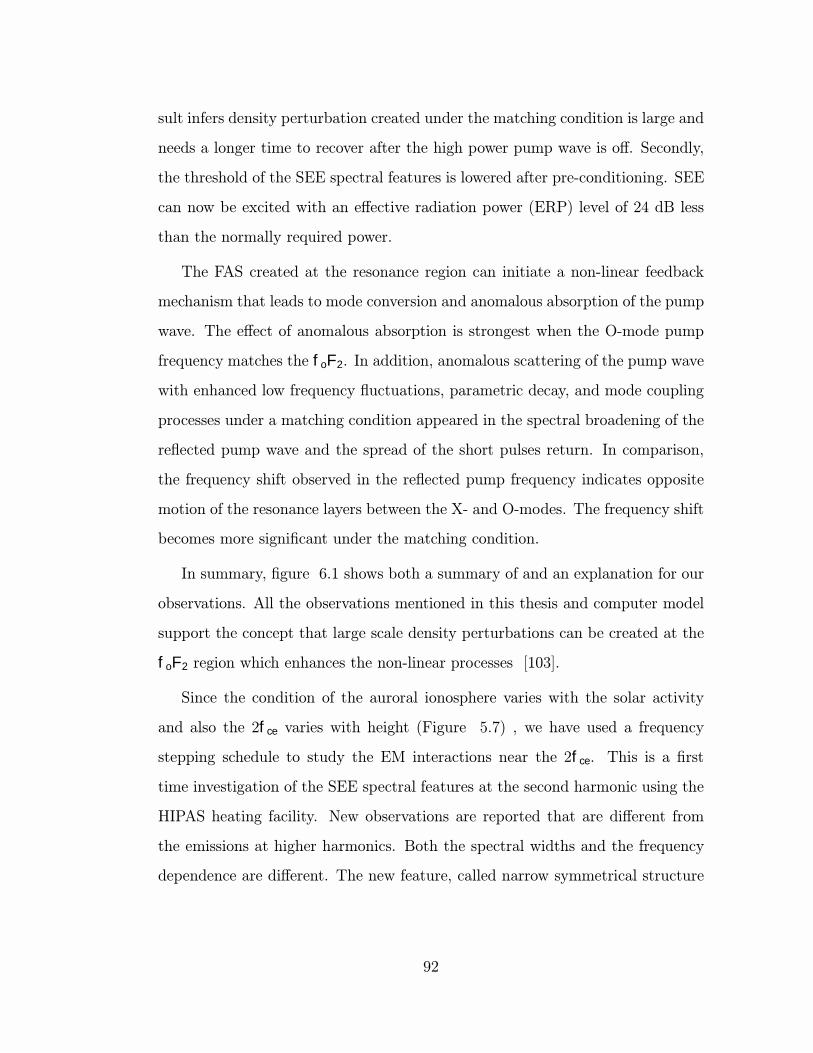
sult infers density perturbation created under the matching condition is large and
needs a longer time to recover after the high power pump wave is off. Secondly,
the threshold of the SEE spectral features is lowered after pre-conditioning. SEE
can now be excited with an effective radiation power (ERP) level of 24 dB less
than the normally required power.
The FAS created at the resonance region can initiate a non-linear feedback
mechanism that leads to mode conversion and anomalous absorption of the pump
wave. The effect of anomalous absorption is strongest when the O-mode pump
frequency matches the foF2. In addition, anomalous scattering of the pump wave
with enhanced low frequency fluctuations, parametric decay, and mode coupling
processes under a matching condition appeared in the spectral broadening of the
reflected pump wave and the spread of the short pulses return. In comparison,
the frequency shift observed in the reflected pump frequency indicates opposite
motion of the resonance layers between the X- and O-modes. The frequency shift
becomes more significant under the matching condition.
In summary, figure 6.1 shows both a summary of and an explanation for our
observations. All the observations mentioned in this thesis and computer model
support the concept that large scale density perturbations can be created at the
foF2 region which enhances the non-linear processes [103].
Since the condition of the auroral ionosphere varies with the solar activity
and also the 2fce varies with height (Figure 5.7) , we have used a frequency
stepping schedule to study the EM interactions near the 2fce. This is a first
time investigation of the SEE spectral features at the second harmonic using the
HIPAS heating facility. New observations are reported that are different from
the emissions at higher harmonics. Both the spectral widths and the frequency
dependence are different. The new feature, called narrow symmetrical structure
92

O-mode CW pump wave
Frequency matching
Large E field enhanced ¶metric instabilities
Local heating & density perturbation
Field aligned striations
Enhancedscattering
Plasma drift motion
Rapid modeconversion
Anomalousabsorption
Skywavedepletion
Frequencybroadening
Echospreading
Dopplershifts
Initial conditions:
Heatingeffects:
Experimentalobservations:
Figure 6.1: Block diagram of a self-consistent physical model to explain the results of
EM wave interact with the ionosphere at the peak of the ionospheric density profile. The
model includes the initial conditions, heating effects, and experimental observations.
93

(NSS), consists of two spectral peaks, symmetrically located around the pump
frequency fpump, at offset frequencies of 15 to 30 kHz. It bears some resemblance
to the broad symmetric structure (BSS) excited at a pump frequency near the
third electron cyclotron harmonics. A simple model is put forward to explain
the generation mechanism of the NSS. We propose the matching of the pump
frequency with the second gyroharmonics accelerate the ionospheric electrons to
higher energy level and interact with the pump to generate the NSS.
Regarding future experimental work, it appears important to further explore
the matching at the second cyclotron harmonic. High time resolution measure-
ments of the evolution of the NSS at the turn-on and turn-off of the pump wave
should be made. The NSS dependence on different propagation direction of the
pump wave should be measured. Particularly along the magnetic field line. A
quantitative analysis and computer modeling are necessary to confirm the model
presented in this thesis.
It would be interesting to match the pump frequency with the second gy-
roharmonic and with the peak of the ionospheric electron density profile, i.e.
fpump = 2fce = foF2.
It is the belief of the author that with improved data taking techniques and
simultaneous measurements of the SEE radiated from the perturbed ionosphere
with several receivers at different locations could provide valuable information on
the physical processes taking place. In particular with the collaborations of other
diagnostic such as the ionosonde, SuperDARN, coherent and incoherent radars.
94

APPENDIX A
Reprint of “Controlled ionospheric
preconditioning and stimulated electromagnetic
radiation” by P. Y. Cheung, A. Y. Wong,
J. Pau, and E. Mjølhus, Phys. Rev. Lett., 80,
4891—4 (1998)
95

VOLUME 80, NUMBER 22 P H Y S I C A L R E V I E W L E T T E R S 1 JUNE 1998
Controlled Ionospheric Preconditioning and Stimulated Electromagnetic Radiation
P. Y. Cheung, A. Y. Wong, and J. PauDepartment of Physics and Astronomy, University of California, Los Angeles, California 90095
E. MjølhusInstitute of Mathematical Sciences, University of Tromsø, N-9037 Tromsø, Norway
(Received 22 January 1998)
New results of stimulated electromagnetic emissions (SEE) from the HIPAS Observatory are reported.A novel hf heating sequence was used to first precondition the ionosphere, and SEE was then excitedwith low-amplitude test pulses. Through this approach, the nonlinear physics of SEE was studied. Thecorrelation between small-scale field-aligned density striations and SEE generation was demonstrated,and SEE was excited at power density of 24 dB less than normally required. The results compare wellwith theoretical predictions of SEE generation via trapped upper hybrid oscillations decay and cavitationwithin striations. [S0031-9007(98)06204-8]
PACS numbers: 94.20.Tt, 52.35.Mw, 52.35.Ra
The ionosphere provides an “outdoor laboratory” [1]ideally suited for the study and excitation of thermaland nonlinear plasma instabilities through high frequency(hf) ionospheric modification experiments. A manifesta-tion of thermal instabilities is the observation of magneticfield-aligned density striations detected via radar scat-tering [2–4] and in situ rocket measurements [5]. Amanifestation of nonlinear plasma processes is the ob-servation of stimulated hf radiation from the heatedionosphere, commonly called stimulated electromagneticemissions (SEE), through frequency analysis of the re-turned hf signal after its transit through the ionosphere[6–16]. Two of the more robust SEE spectral featuresobserved under high duty cycle hf heating are a broad,diffuse, and down-shifted (with respect to the heating fre-quency,fhf) continuum, with frequency extension of tensof kilohertz or more, called the broad continuum; anda discrete, narrow, down-shifted peak, called the down-shifted maximum, with an offset frequency near the lowerhybrid frequency,flh [11,12].
It has been suggested that these SEE features are asso-ciated with the occurrence of heater-induced small-scale(meter-size) striations [17–21] which act as resonatorsfor electrostatic oscillations at the upper hybrid frequency,fuh. In contrast to Langmuir oscillations near the reflec-tion layer wherefhf � fp�zo� [ fp�zo� is the plasma fre-quency at the reflection layerzo ], these oscillations havewave vectors predominantly perpendicular to the ambi-ent magnetic field. Recently, Mjølhus [22,23] proposes aSEE theory including the presence of striations and hascalculated the radiation source current spectra. Trappedupper hybrid oscillations or eigenstates, with frequencyof f � fhf � fuh�z�, are first generated via conversionof pump wave off meter-size striations. The parametricdecay of these states, withf 0 � fhf 2 fdm (f 0 is thedecay wave frequency), results in the generation of thedown-shifted maximum feature. Optimum growth of thistrapped upper hybrid decay instability is predicted to oc-
cur when the frequency offset,fdm � fhf 2 f 0�, is nearflh. The resultant radiation source current spectrum con-tains discrete spectral peaks that can be identified with thedown-shifted maximum feature. As the pump field in-creases, the discrete peaks change to a broad diffuse con-tinuum. A new cavitation process within the striations hasalso been suggested for the generation of the broad con-tinuum feature.
The physics of nonlinear SEE generation, in short, en-compasses fundamental processes such as the conversionof electromagnetic waves to electrostatic waves off stria-tions, the excitation of trapped eigenmodes, parametric in-stabilities, and stimulated radiation of electrostatic waves.These issues are topics of active research not only in iono-spheric experiments but also in laboratory studies. It is ofgeneral interest and great importance, then, that these is-sues be studied in relation to SEE, that the correlation ofstriations and SEE be demonstrated, and that details oftheoretical predictions be tested under controlled experi-ments. A survey of past experiments, however, yields in-conclusive results.
In this Letter, new results of SEE from a series of con-trolled ionospheric preconditioning experiments are pre-sented. Specifically, our experimental procedure allows(i) each heating sequence to initiate from or to approachthat of a cold start condition; (ii) the complete historyof temporal evolution of SEE, from its initial growthto its long-time evolution, be recorded; (iii) the correla-tion of striations and SEE be clearly demonstrated; and(iv) the low threshold requirement of SEE generation viathe trapped upper hybrid decay instability and cavitationbe verified. Our results demonstrate unambiguously that,in a preconditioned ionosphere with striations, SEE fea-ture such as the down-shifted maximum can be excitedand observed readily with test hf pulses that can be 24 dBweaker in power density than normally required withoutpreconditioning. We have also found that the most dra-matic data were observed under the conditions when hf
0031-9007�98�80(22)�4891(4)$15.00 © 1998 The American Physical Society 4891
96

VOLUME 80, NUMBER 22 P H Y S I C A L R E V I E W L E T T E R S 1 JUNE 1998
FIG. 1. Schematic of one heating sequence. The sequenceconsisted of a series of test pulses (T1, T2, and T3) at aneffective radiated power �80 kW, two heating pump pulses(H1 and H2) at �20 MW, and a cooling period.
heater pump frequency, fhf, is near the maximum plasmafrequency, foF2, of the ionosphere [24,25].
To accomplish our objectives, a novel heating sequencewas used instead of transmitting at maximum powercontinuously. Figure 1 shows one cycle of the heatingsequence (10 min long) consisting of three series of shorttest pulses (T1, T2, and T3), two main heating pumppulses (H1 and H2), and a long cooling period. Eachseries of test pulses further consisted of three separatepulses (10 s each) at three different test frequencies.Test pulses, T1, were first transmitted to check thebackground ionospheric conditions and to ensure a coldstart condition, i.e., a clean ionosphere with no priorheating effects. This was accomplished by monitoringthe spectra of returned signals of test pulses at multiplefrequencies. The duration of each pump pulse, 136 s,was chosen to facilitate the growth of small-scale (meter-size) striations while avoiding the excitation of largerscale perturbations. The effects of heating from the firstpump pulse, H1, were monitored by a second sequenceof test pulses, T2, and the effects of H2, which can alsobe considered as a test pulse with large amplitude, weremonitored by a final sequence of test pulses, T3. Theheating cycle was then repeated after the long coolingperiod of 200 s when all hf transmission was off.
Experiments were performed periodically from late Feb-ruary to early November 1997 at HIPAS Observatory [26].The results presented here were selected from the Juneexperiment and are representative of the overall data col-lected. Measurements of returned hf waves were made atthe NOAA facility at Gilmore Creek, 33 km away fromthe HIPAS Observatory. For this particular set of experi-ments, the effective radiated power of the main heaterwave was �20 MW while that of the test pulses was�80 kW. Both the transmitted main pump wave withfhf � 4.53 MHz and the test pulses with frequencies offt � 4.50, 4.53, and 4.56 MHz were at ordinary (O) modepolarization. These heating and test frequencies were nearfoF2 but were sufficiently away from the nearest multiplesof electron cyclotron frequency fce that gyroharmonic ef-fects are minimized [10]. Specifically, � fhf, ft� 2 3fce .300 kHz at the reflection layer of �220 km.
FIG. 2. Temporal evolution of returned hf signal of the firstpump pulse H1 which shows a gradual decline (top panel) andthe SEE signal at 29 kHz from fhf which shows a gradualincrease (bottom panel).
The temporal evolution of the returned hf power ofpump H1 and its spectral (or SEE) power at a down-shifted frequency of 29 KHz are shown in Fig. 2. Coldstart condition was first confirmed by monitoring thereturn of T1 [see Fig. 4(a)]. After turn-on at t � 2 s, thereturn pump signal (top panel) drop 10 dB from a range of�72 dB to a range of �62 dB within a span of 20 s. Thisdrop in return pump strength is generally attributed to theanomalous absorption of the pump signal as a result ofthe formation of striations and the subsequent scatteringand conversion of pump wave to electrostatic oscillations[10,27–29]. The SEE signal at 29 kHz (bottom panel),on the other hand, displays a rapid rise within the first10–15 s after turn-on. These two figures clearly showthat the growth of SEE is correlated with the decline ofpump signal and the excitation of striations.
Sample spectra of returned hf signal of pump H1
at two discrete times, one near turn-on and the other88 s into the heating pulse, are shown in Figs. 3(a) and3(b), respectively. Following past convention, the broaddiffuse structure extending from the pump signal peakto negative frequencies is labeled the broad continuum,while the broad peak riding on the continuum at about9–10 kHz is labeled the down-shifted maximum. Thecenter frequency of the down-shifted maximum featureis close to the lower hybrid frequency of flh � 8 kHz.Comparison of Figs. 3(a) and 3(b) illustrates the relativelyslow growth of SEE during this first heating periodinitiating from cold start. For this set of data, the down-shifted maximum feature is barely noticeable in Fig. 3(b).
Preconditioning by pump H1 makes a significant impacton subsequent test pulse results. This is illustratedby the difference in SEE spectra of returned signalsof test pulses T1 and T2 before and after H1 shown
4892
97

VOLUME 80, NUMBER 22 P H Y S I C A L R E V I E W L E T T E R S 1 JUNE 1998
FIG. 3. Frequency spectra of returned hf signal of first pumppulse H1. Panel (a) shows the spectrum near turn-on of H1.Panel (b) shows the spectrum 88 s into heating. The horizontalfrequency scale is offset from fhf.
in Figs. 4(a) and 4(b) for ft � 4.56 MHz. Figure 4(a)shows, as expected, no SEE from the turn signal of T1.This is consistent with the cold start condition and theresult of the much reduced effective radiated power of80 kW. After preconditioning, however, the results arevery different. Figure 4(b) shows a sample spectrum fromthe return signal of T2 transmitted 4 s after H1 was turnedoff. First, good SEE was observed even at the reducedradiated power. Second, the spectrum shows a very strongand discrete down-shifted maximum feature. This is indistinct contrast to the down-shifted maximum featuresobserved from main pump pulses H1 and H2 which arefrequently superposed on a continuum background. Thediscreteness of the down-shifted maximum feature alsoappears to be more robust when fhf � foF2.
Preconditioning effects can also persist past the turn-on time of second pump pulse H2 (transmitted 44 s afterH1 is shut off), and the results are shown in Fig. 5.The returned power of H2 (top panel), in contrast tothat from H1 shown in Fig. 2, is at a depressed level of�62 dB due to anomalous absorption from preexistingstriations immediately at turn-on, and remains depressedthroughout the heating period. The evolution of SEEpower at 29 KHz (bottom panel) is also in contrast tothat of H1. It has a strong overshoot at turn-on which is
FIG. 4. Frequency spectra of returned signal of test pulses T1and T2. Panel (a) shows no SEE for T1 before H1. Panel (b)shows SEE with a discrete down-shifted maximum feature forT2 after H1. The frequency scale on each panel is offset fromft � 4.56 MHz.
followed by a quick drop with the signal level settling intothe same range as that during H1. This overshoot is veryreproducible and occurs consistently during the secondheating period with the combination of a large heatingpump and preexisting striations.
The overshoot also leads to large frequency broadeningin SEE spectra of return signal of second pump H2.Figure 6(a) shows the spectrum during the overshoot.It shows strong SEE that has a relatively sharp down-shifted maximum peak riding on top of a very broadcontinuum with frequency extension of over 30 kHz.Figure 6(b) shows the spectrum 9 s into the heatingperiod. It shows weaker SEE with a broader down-shiftedmaximum peak riding on a much narrower continuumbackground. Comparison of the two sets of spectra shownin Figs. 3 and 6 clearly contrasts the systematic growthof SEE from cold start condition with pump H1 andthe overshoot phenomenon of SEE with pump H2 afterpreconditioning.
Many of our observed results can now be comparedwith theoretical predictions of Mjølhus [22,23] and beexplained. First, the presence of meter-size striation isrequired in the model. As pointed out earlier, this isinferred experimentally with results from H1 where thegrowth of the SEE signal is correlated with the anomalousdecay of the pump signal [10,27–29]. Second, the modelpredicts a very low threshold for the excitation of trappedunder hybrid decay instability. This is confirmed byour test pulses data that show the power threshold canbe more than 20 dB lower with respect to H1 andH2 that generate the striations. Converting experimentalparameters into the same scaled units as in the modeland comparing with the instability threshold, the test
FIG. 5. Temporal evolution of returned hf signal of secondpump pulse H2 (top panel) and the SEE signal at 29 kHz fromfhf (bottom panel) that shows a strong overshoot immediatelyafter turn-on.
4893
98
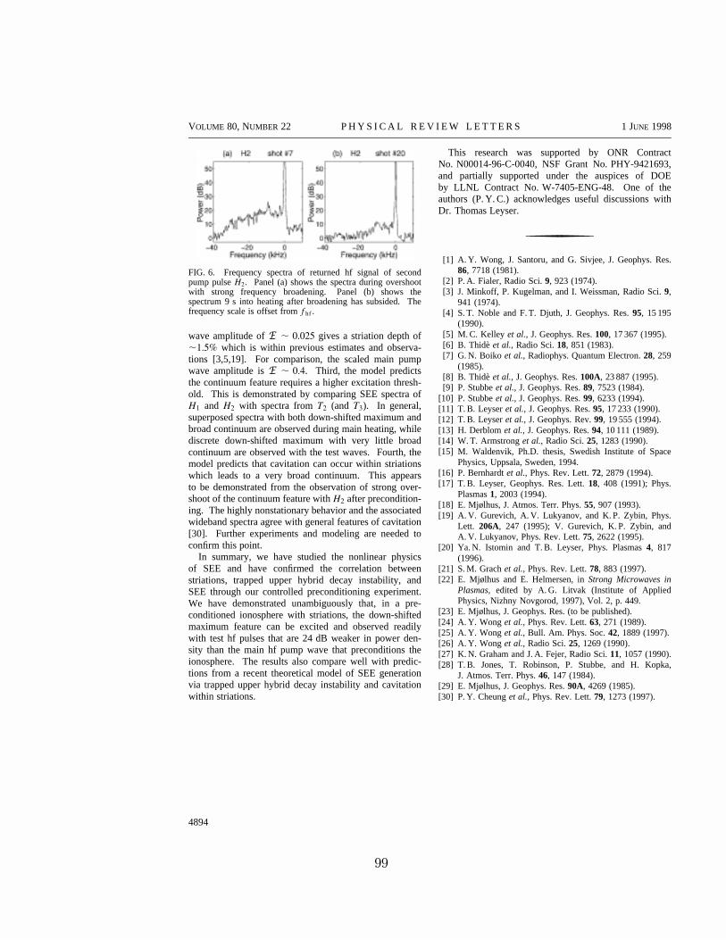
VOLUME 80, NUMBER 22 P H Y S I C A L R E V I E W L E T T E R S 1 JUNE 1998
FIG. 6. Frequency spectra of returned hf signal of secondpump pulse H2. Panel (a) shows the spectra during overshootwith strong frequency broadening. Panel (b) shows thespectrum 9 s into heating after broadening has subsided. Thefrequency scale is offset from fhf.
wave amplitude of E � 0.025 gives a striation depth of�1.5% which is within previous estimates and observa-tions [3,5,19]. For comparison, the scaled main pumpwave amplitude is E � 0.4. Third, the model predictsthe continuum feature requires a higher excitation thresh-old. This is demonstrated by comparing SEE spectra ofH1 and H2 with spectra from T2 (and T3). In general,superposed spectra with both down-shifted maximum andbroad continuum are observed during main heating, whilediscrete down-shifted maximum with very little broadcontinuum are observed with the test waves. Fourth, themodel predicts that cavitation can occur within striationswhich leads to a very broad continuum. This appearsto be demonstrated from the observation of strong over-shoot of the continuum feature with H2 after precondition-ing. The highly nonstationary behavior and the associatedwideband spectra agree with general features of cavitation[30]. Further experiments and modeling are needed toconfirm this point.
In summary, we have studied the nonlinear physicsof SEE and have confirmed the correlation betweenstriations, trapped upper hybrid decay instability, andSEE through our controlled preconditioning experiment.We have demonstrated unambiguously that, in a pre-conditioned ionosphere with striations, the down-shiftedmaximum feature can be excited and observed readilywith test hf pulses that are 24 dB weaker in power den-sity than the main hf pump wave that preconditions theionosphere. The results also compare well with predic-tions from a recent theoretical model of SEE generationvia trapped upper hybrid decay instability and cavitationwithin striations.
This research was supported by ONR ContractNo. N00014-96-C-0040, NSF Grant No. PHY-9421693,and partially supported under the auspices of DOEby LLNL Contract No. W-7405-ENG-48. One of theauthors (P. Y. C.) acknowledges useful discussions withDr. Thomas Leyser.
[1] A. Y. Wong, J. Santoru, and G. Sivjee, J. Geophys. Res.86, 7718 (1981).
[2] P. A. Fialer, Radio Sci. 9, 923 (1974).[3] J. Minkoff, P. Kugelman, and I. Weissman, Radio Sci. 9,
941 (1974).[4] S. T. Noble and F. T. Djuth, J. Geophys. Res. 95, 15 195
(1990).[5] M. C. Kelley et al., J. Geophys. Res. 100, 17 367 (1995).[6] B. Thidè et al., Radio Sci. 18, 851 (1983).[7] G. N. Boiko et al., Radiophys. Quantum Electron. 28, 259
(1985).[8] B. Thidè et al., J. Geophys. Res. 100A, 23 887 (1995).[9] P. Stubbe et al., J. Geophys. Res. 89, 7523 (1984).
[10] P. Stubbe et al., J. Geophys. Res. 99, 6233 (1994).[11] T. B. Leyser et al., J. Geophys. Res. 95, 17 233 (1990).[12] T. B. Leyser et al., J. Geophys. Rev. 99, 19 555 (1994).[13] H. Derblom et al., J. Geophys. Res. 94, 10 111 (1989).[14] W. T. Armstrong et al., Radio Sci. 25, 1283 (1990).[15] M. Waldenvik, Ph.D. thesis, Swedish Institute of Space
Physics, Uppsala, Sweden, 1994.[16] P. Bernhardt et al., Phys. Rev. Lett. 72, 2879 (1994).[17] T. B. Leyser, Geophys. Res. Lett. 18, 408 (1991); Phys.
Plasmas 1, 2003 (1994).[18] E. Mjølhus, J. Atmos. Terr. Phys. 55, 907 (1993).[19] A. V. Gurevich, A. V. Lukyanov, and K. P. Zybin, Phys.
Lett. 206A, 247 (1995); V. Gurevich, K. P. Zybin, andA. V. Lukyanov, Phys. Rev. Lett. 75, 2622 (1995).
[20] Ya. N. Istomin and T. B. Leyser, Phys. Plasmas 4, 817(1996).
[21] S. M. Grach et al., Phys. Rev. Lett. 78, 883 (1997).[22] E. Mjølhus and E. Helmersen, in Strong Microwaves in
Plasmas, edited by A. G. Litvak (Institute of AppliedPhysics, Nizhny Novgorod, 1997), Vol. 2, p. 449.
[23] E. Mjølhus, J. Geophys. Res. (to be published).[24] A. Y. Wong et al., Phys. Rev. Lett. 63, 271 (1989).[25] A. Y. Wong et al., Bull. Am. Phys. Soc. 42, 1889 (1997).[26] A. Y. Wong et al., Radio Sci. 25, 1269 (1990).[27] K. N. Graham and J. A. Fejer, Radio Sci. 11, 1057 (1990).[28] T. B. Jones, T. Robinson, P. Stubbe, and H. Kopka,
J. Atmos. Terr. Phys. 46, 147 (1984).[29] E. Mjølhus, J. Geophys. Res. 90A, 4269 (1985).[30] P. Y. Cheung et al., Phys. Rev. Lett. 79, 1273 (1997).
4894
99

References
[1] W. T. Armstrong, R. Massey, P. Argo, R. Carlos, D. Riggin, P. Y. Cheung,M. McCarrick, J. Stanley, and A. Y. Wong. Continuous measurement ofstimulated electromagnetic emission spectra from hf excited ionosphericturbulence. Radio Sci., 25:1283—1289, 1990.
[2] B. S. Bauer, A. Y. Wong, L. Scurry, and V. K. Decyk. Efficiency of cavitonformation as a function of plasma density gradient. Physics of Fluids B(Plasma Physics), 2(8):1941—1943, 1990.
[3] V. N. Belyakova, I. V. Berezin, V. V. Vas kov, Yu. V. Gruzdev, Yu. S. Di-mant, V. A. Zyuzin, O. P. Kapustina, G. P. Komrakov, L. A. Lobachevskiy,G. A. Mikhaylova, V. A. Panchenko, V. P. Polimatidi, A. V. Prokof ev,V. A. Puchkov, and V. Ryzhov. The features of excitation of plasma tur-bulence by a high-power radio wave field under even-order gyroresonanceconditions. Geomagn. Aeron., 31:367—370, 1991.
[4] I. V. Berezin, V. B. Belyanskiy, N. I. Bud ko, V. V. Vas kov, Yu. S. Dimant,V. A. Zyuzin, O. P. Kapustina, G. P. Komrakov, L. A. Lobachevskiy, G. A.Mikhaylova, V. A. Panchenko, A. V. Prokof ev, and V. Ryzhov. Diagnosticsof processes of excitation of plasma oscillations by the field of a powerfulradio wave. Geomagn. Aeron., 31:702—706, 1991.
[5] P. A. Bernhardt, M. Wong, J. D. Hube, B. G. Fejer, L. S. Wagner, J. A.Goldstein, C. A. Selcher, V. L. Frolov, and E. N. Sergeev. Optical remotesensing of the thermosphere with hf pumped artificial airglow. J. Geophys.Res., 105:10,657—10,671, 2000.
[6] N. F. Blagoveshchenskaya, V. A. Kornienko, M. T. Rietveld, B. Thide,A. Brekke, I. V. Moskvin, and S. Nozdrachev. Stimulated emissions aroundsecond harmonic of troms heater frequency observed by long-distance di-agnostic hf tool. Geophys. Res. Lett., 25(6):873—876, 1998.
[7] G. N. Boiko, L. M. Erukhimov, V. A. Zyuzin, G. P. Komrakov, S. A.Metelev, N. A. Mityakov, V. A. Nikonov, V. A. Ryzhov, Yu. V. Tokarev,and V. L. Frolov. Dynamic characteristics of stimulated radio emission fromionospheric plasma. Radiophys. Quantum Electron. Engl. Transl., 28:259—268, 1985.
[8] K. G. Budden. The propagation of radio waves. Cambridge UniversityPress, London, 1985.
100

[9] H. C. Carlson, W. E. Gordon, and R. L. Showen. High frequency inducedenhancements of the incoherent scatter spectrum at arecibo. J. Geophys.Res., 77:1242—1250, 1972.
[10] J. Carroll, E. Violette, and W. Utlaut. The platteville high power facility.Radio Sci., 9:889—894, 1974.
[11] P. Y. Cheung, D. F. DuBois, T. Fukuchi, K. Kawan, H. A. Rose, D. Russell,T. Tanikawa, and A. Y. Wong. Investigation of strong langmuir turbulencein ionospheric modification. J. Geophys. Res., 97:10,575—10,600, 1992.
[12] P. Y. Cheung, E. Mjølhus, D. F. DuBois, J. Pau, H. Zwi, and A. Y. Wong.Stimulated radiation from strong langmuir turbulence in ionospheric mod-ification. Phys. Rev. Lett., 79:1273—1276, 1997.
[13] P. Y. Cheung, A. Y. Wong, J. Pau, and E. Mjølhus. Controlled ionosphericpre-conditioning and stimulated electromagnetic radiation. Phys. Rev.Lett., 80:4891—4894, 1998.
[14] R. A. Close, B. S. Bauer, A. Y. Wong, A. B. Langdon, W. L. Kruer, andE. Mjølhus. Computer simulation of ionospheric radio frequency heating.Radio Sci., 25(6):1341—1349, 1990.
[15] R. Cohen and J. D. Whitehead. Radio-reflectivity detection of artificialmodification of the ionospheric f layer. J. Geophys. Res., 75:6439—6445,1970.
[16] K. Davies. Ionospheric Radio Waves. Blaisdell Publishing Company, 1969.
[17] D. F. DuBois and M. V. Goldman. Radiation induced instability of electronplasma oscillations. Phys. Rev. Lett., 14:544, 1965.
[18] J. R. Dudeney and M. J. Jarvis. A simple graphical method for dealiasingdigital ionosonde echo location data. Radio Sci., 21:101—105, 1986.
[19] M. H. Jarvisand J. R. Dudeney. Reduction of ambiguities in hf radar resultsthrough a revised receiving antenna array and sounding pattern. Radio Sci.,21:151—158, 1986.
[20] L. M. Duncan and W. E. Gordon. Ionospheric modification by high powerradio waves. J. Atmos. Terr. Phys., 44:1009—1017, 1982.
[21] K. B. Dysthe, E. Mjølhus, H. Pecseli, and K. Rypdal. Thermal cavitons.Physica Scripta, T2/2:548—559, 1982.
101

[22] L. M. Erukhimov, S. A. Metelev, E. N. Myasnikov, N. A. Mityakov, andV. L. Frolov. Artificial ionospheric turbulence (review). Radiophys. Quan-tum Electron. Engl. Transl., 30:156—171, 1987.
[23] J. A. Fejer. Generation of large-scale field-aligned density irregularitiesin ionospheric heating experiments. In AGARD Conf. Proc., volume 138,pages 13—1 — 13—6, 1973.
[24] J. A. Fejer. Ionospheric modification and parametric instabilities. Reviewsof Geophysics and Space Physics, 17(1):135—53, 1979.
[25] J. A. Fejer and Y. Y. Kuo. Structure in the nonlinear saturation spectrumof parametric instabilities. Phys. Fluids, 16:1490, 1973.
[26] P. A. Fialer. Field-aligned scattering from a heated region of the ionosphereobservations at hf and vhf. Radio Sci., 9:923—940, 1974.
[27] V. L. Frolov, G. N. Boiko, S. A. Metelev, and E. N. Sergeev. On the studyof artificial ionospheric turbulence by means of stimulated electromagneticemission. Radiophys. Quantum Electron. Engl. Transl., 37:593—603, 1994.
[28] V. L. Frolov, E. N. Ermakova, L. M. Erukhimov, G. P. Komrakov, E. N.Sergeev, and P. Subbe. A new upshifted spectral stimulated electromag-netic emission strcture, observed between electron cyclotron harmonics.GRL, 24:1647—1650, 1997.
[29] V. L. Frolov, E. N. Ermakova, L. M. Kagan, G. P. Komrakov, E. N. Sergeev,and P. Subbe. Features of the broad upshifted structure in stimulatedelectromagnetic emission spectra. JGR, 105:20919—20933, 2000.
[30] V. L. Frolov, E. N. Ermakova, L. M. Kagan, G. P. Komrakov, S. N. Sergeev,and P. Stubbe. Features of the broad upshifted structure in stimulated elec-tromagnetic emission spectra. J. Geophys. Res., 105(A9):20919—33, 2000.
[31] V. L. Frolov, L. M. Erukhimov, S. A. Metelev, and S. N. Sergeev. Tempo-ral behaviour of artificial small-scale ionospheric irregularities: Review ofexperimental results. J. Atmos. Sol. Terr. Phys., 59(18):2317—2333, 1997.
[32] V. L. Frolov, S. M. Grach, L. M. Erukhimov, G. P. Komrakov, E. N.Sergeev, B. Thide, and T. Carozzi. Preculiarities in the evolution of thebum of stimulated radio emission of the ionosphere. Radiophys. QuantumElectron, 39:241—254, 1996.
[33] V. E. Golant and A. D. Piliya. Linear transformation and absorption ofwaves in a plasma. Sov. Physics. Uspekhi, 14:413—437, 1972.
102

[34] W. E. Gordon, R. Showen, and H. C. Carlson. Ionospheric heating atarecibo: First test. J. Geophys. Res., Space Phys., 75:6436—6438, 1971.
[35] S. M. Grach. Electromagnetic radiation from artificial ionospheric plasmaturbulence. Radiophys. Quantum Electron. Engl. Transl., 28:470—477, 1985.
[36] S. M. Grach, M. M. Shvarts, E. N. Sergeev, and V. L. Frolov. Broadcontinuum feature of stimulated electromagnetic emission. J. Atmos. Sci.,60:1233—1246, 1998.
[37] K. N. Graham and J. A. Fejer. Anomalous raio wave absorption due toionospheric heating effects. Radio Sci., 11:1057—1063, 1976.
[38] A. V. Gurevich. Nonlinear phenomena in the ionosphere. Springer-Verlag,New York, 1978.
[39] A. V. Gurevich, H. Carlson, A. V. Lukyanov, and K. P. Zybin. Parametricdecay of upper hybrid plasma waves trapped inside density irregularities inthe ionosphere. Phys. Letts. A, 23:97—108, 1997.
[40] A. V. Gurevich, A. V. Lukyanov, and K. P.Zybin. Stationary state ofisolated striations developed during ionospheric modification. Phys. Lett.A, 206:247—259, 1995.
[41] A. V. Gurevich, A. V. Lukyanov, and K. P.Zybin. Anomalous absorp-tion of powerful radio waves on the striations developed during ionosphericmodification. Phys. Lett. A, 211:363—372, 1996.
[42] A. V. Gurevich, K. P. Zybin, and A. V. Lukyanov. Stationary striationdeveloped in the ionospheric modification. Phys. Rev. Lett., 75(13):2622—2625, 1995.
[43] P. N. Guzdar, P. K. Chaturvedi, K. Papadopoulos, M. J. Keskinen, andS. L. Ossakow. The self-focusing instability in the presence of density ir-regularities in the ionosphere. J. Geophys. Res., 101:2453—2460, 1996.
[44] P. N. Guzdar, P. K. Chaturvedi, K. Papadopoulos, and S. L. Ossakow. Thethermal self-focusing instability near the critical surface in the high-latitudeionosphere. J. Geophys. Res., 103:2231—2237, 1998.
[45] T. Hagfors, W. Kofman, H. Kopka, P. Stubbe, and T. Aijanen. Observa-tions of enhanced plasma lines by eiscat during heating experiments. RadioSci., 18:861—866, 1983.
103

[46] A. Hedberg, H. Derblom, B. Thide, H. Kopka, and P. Stubbe. Observationsof hf backscatter associated with the heating experiment at tromsø. RadioSci., 18:840—850, 1983.
[47] D. E. Hinkel-Lipsker, B. D. Fried, and G. J. Morales. Analytic expressionfor mode conversion of langmuir and electromagnetic waves. Phys. Rev.Lett., 62:2680—2682, 1989.
[48] F. Honary, A. J. Stocker, T. R. Robinson, T. B. Jones, and P. Stubbe.Ionospheric plasma response to hf radio waves operating at frequenciesclose to the third harmonic of the electron gyrofrequency. J. Geophys.Res., 100(A11):21489—501, 1995.
[49] R. D. Hunsucker. Radio Techniques for Probing the Terrestrial Ionosphere,volume 22 of Physics and Chemistry in Space. Springer-Verlag Berlin Hei-delberg, 1991.
[50] Ya. N. Istomin and T. B. Leyser. Small-scale magnetic field-aligned densityirregularities excited by a powerful electromagnetic wave. Phys. Plasmas,4(3):817—828, 1997.
[51] Ya. N. Istomin and T. B. Leyser. Parametric interaction of self-localizedupper hybrid states in quantized plasma density irregularities. Phys. Plas-mas, 5(4):921—931, 1998.
[52] Ya. N. Istomin and T. B. Leyser. Quantization of plasma density irregu-larities under the action of a powerful electromagnetic wave: Spectrum ofupper hybrid oscillations self consistently trapped in the density cavities.Radiophys. Quantum Electron. Engl. Transl., 42:641—650, 1999.
[53] T. B. Jones, T. Robinson, P. Stubbe, and H. Kopka. Frequency dependenceof anomalous absorption caused by high power radio waves. J. Atmos. Terr.Phys., 46:147—153, 1984.
[54] W. L. Kruer. Model of resonance absorption with profile modification.Phys. Fluids, 25(12):2324—2325, 1982.
[55] W. L. Kruer. The Physics of Laser Plasma Interactions. Addison-WesleyPublishing Company, New York, 1988.
[56] T. B. Leyser, B. T hide, M. Waldenvik, S. Goodman, V. L. Frolov, S. M.Grach, A. N. Karashtin, G. P. Komrakov, and D. S. Kotik. Spectral struc-ture of stimulated electromagnetic emissions between electron cyclotronharmonics. J. Geophys. Res., 98(A10):17597 — 17606, 1993.
104

[57] T. B. Leyser, B. Thide, H. Derblom, A. Hedberg, B. Lundborg, P. Stubbe,and H. Kopka. Stimulated electromagnetic emission near electron cyclotronharmonics in the ionosphere. Phys. Rev. Lett., 63:1145—147, 1989.
[58] T. B. Leyser, B. Thide, H. Derblom, A. Hedberg, B. Lundborg, P. Stubbe,and H. Kopka. Dependence of stimulated electromagnetic emission on theionosphere and pump wave. J. Geophys. Res., 95:17,233—17,244, 1990.
[59] T. B. Leyser, B. Thide, S. Goodman, M. Waldenvik, E. Veszelei, S. M.Grach, A. N. Karashtin, G. P. Komrakov, and D. S. Kotik. Narrow cy-clotron harmonic absorption resonances of stimulated electromagnetic emis-sion in the ionosphere. Phys. Rev. Lett., 68:3299—3302, 1992.
[60] T. B. Leyser, B. Thide, M. Waldenvik, E. Veszelei, V. L. Frolov, S. M.Grach, and G. P. Komrakov. Downshifted maximum features in stimu-lated electromagnetic emission spectra. J. Geophys. Res., 99(A10):19,555—19,568, 1994.
[61] B. Lundborg and B. Thide. Standing wave pattern of hf radio waves in theionospheric reflection region: 1. general formulas. Radio Sci., 20:947—958,1985.
[62] B. Lundborg and B. Thide. Standing wave pattern of hf radio waves in theionospheric reflection region 2. applications. Radio Sci., 21:486—500, 1986.
[63] G. M. Milikh, K. Papadopoulos, M. McCarrick, and J. Preston. Elf emissiongenerated by the haarp hf-heater using varying frequency and polarization.Radiophys. Quantum Electron. Engl. Transl., 42:639—46, 1999.
[64] J. Minkoff. Radio frequency scattering from a heated ionospheric volume,3, cross-section calculations. Radio Sci., 9:997—1004, 1974.
[65] J. Minkoff, P. Kugelman, and I. Weissman. Radio frequency scatteringfrom a heated ionospheric volume, 1, vhf/uhf field-aligned and plasma-linebackscatter measurements. Radio Sci., 9:941—955, 1974.
[66] E. Mjølhus. Anomalous absorption and reflection in ionospheric radio mod-ification experiments. J. Geophys. Res., 90:4269—4279, 1985.
[67] E. Mjølhus. On linear conversion in a magnetized plasma. Radio Sci.,25:1321—1339, 1990.
[68] E. Mjølhus. Parametric instabilities of trapped upper-hybrid oscillations.J. Plasma Phys., 58:747—769, 1997.
105

[69] E. Mjølhus. Theoretical model for long time stimulated electromagneticemission generation in ionospheric radio modification experiments. J. Geo-phys. Res., 103:14711—14729, 1998.
[70] E. Mjølhus and T. Fla. Direct access to plasma resonance in ionosphericradio experiments. J. Geophys. Res., 89:3921—3928, 1984.
[71] F. W. Perkins, C. Oberman, and E. J. Valeo. Parametric instabilities andionospheric modification. J. Geophys. Res., 79:1478—1496, 1974.
[72] H. Rishbeth and O. K. Garriot. Introduction to ionospheric physics. Aca-demic Press, NewYork and London, 1969.
[73] P. A. Robinson. Nonlinear wave collapse and strong turbulence. Rev. Mod.Phys., 69:507—573, 1997.
[74] P. E. Rodriguez, J. E. Kennedy, M. Keskinen, C. Siefring, Sa. Basu, M. Mc-Carrick, J. Preston, M. Engebretson, M. Kaiser, M. Desch, K. Goetz, J. L.Bougeret, and R. Manning. The wind-haarp experiment: Initial results ofhigh power radiowave interactions with space plasmas. Geophys. Res. Lett.,26:2351—2354, 1999.
[75] D. D. Sentman, R. F. Wuerker, M. J. McCarrick, T. Pedersen, E. M.Wescott, H. Stenbaek-Nielsen, A. Y. Wong, M. Kubota, F. T. Sao Sab-bas, and D. Lummerzheim. Imaging and spectrographic observations ofartificial airglow excited by haarp and hipas. In RF Ionospheric Interac-tions Workshop, page 632, Santa Fe, New Mexico, 2002.
[76] M. M. Shvarts and S. M. Grach. Interaction of upper and lower hybridwaves and generation of the downshifted maximum feature of stimulatedelectromagnetic emissions. J. Atmos. Terr. Phys., 59:2421—2429, 1997.
[77] M. M. Shvarts, S. M. Grach, V. L. Frolov, and E. N. Sergeev. Modelingof the wideband component of artificial radioemission of the ionosphere.Radiophys. Quantum Electron. Engl. Transl., 37:412—431, 1994.
[78] M. M. Shvarts, S. M. Grach, V. L. Frolov, and E. N. Sergeev. On the gener-ation of the stimulated electromagnetic emission. the computer simulationresults. Adv. Space Res., 15:59—62, 1995.
[79] V. P. Silin. Parametric resonance in a plasma. Sov. Phys. JETP, Engl.Transl., 21:1127, 1965.
106

[80] R. L. Stenzel, A. Y. Wong, and H. C. Kim. Conversion of electromagneticwaves to electrostatic waves in inhomogeneous plasmas. Phys. Rev. Lett.,32:654—657, 1974.
[81] A. J. Stocker, F. Honary, T. R. Robinson, and T. B. Jones. Anomalousabsorption during artificial modification at harmonics of the electron gy-rofrequency. J. Geophys. Res., 98:13627—13645, 1993.
[82] P. Stubbe, H. Hopka, B. Thide, and H. Derblom. Stimulated electromag-netic emission: A new technique to study the parametric decay instabilityin the ionosphere. J. Geophys. Res., 89:7523—7536, 1984.
[83] P. Stubbe and H. Kopka. Stimulated electromagnetic emission in a magne-tized plasma: A new symmetric spectral feature. Phys. Rev. Lett., 65:183—186, 1990.
[84] P. Stubbe, H. Kopka, T. B. Jones, and T. Robinson. Wide band attenuationof radio waves caused by powerful hf waves: Saturation and dependence onionospheric variability. J. Geophys. Res., 87:1551—1555, 1982.
[85] P. Stubbe, H. Kopka, H. Lauche, M. T. Rieveld, A. Biekke, O. Holt,T. Robinson T. B. Jones, A. Hedberg, B. Thide, M Crocketr, and H. J. Lotz.Ionospheric modification experiments in northern scandinavia. J. Atmos.Terr. Phys., 44:1025—1041, 1982.
[86] P. Stubbe, A. J. Stocker, F. Honary, T. R. Robinson, and T. B. Jones.Stimulated electromagnetic emissions and anomalous hf wave absorptionnear electron gyroharmonics. J. Geophys. Res., 99(A4):623—6246, 1994.
[87] B. Thide, H. Derblom, A. Hedberg, H. Kopka, and P. Stubbe. Observationsof stimulated electormagnetic emissions in ionospheric heating experiments.Radio Sci., 18:851—859, 1983.
[88] B. Thide, F. T. Djuth, T. B. Leyser, and H. M. Ierkic. Evolution of langmuirturbulence and stimulated electromagnetic emissions excited with a 3-mhzpump wave at arecibo. J. Geophys. Res., 100(A12):23887—23899, 1995.
[89] B. Thide, A. Hedberg, J. A. Fejer, and M. P. Sulzer. First observationsof stimulated electromagnetic emission at arecibo. Geophys. Res. Lett.,16:369—372, 1989.
[90] B. Thide, H. Kopka, and P. Stubbe. Observations of stimulated scatteringof a strong high-frequency radio wave in the ionosphere. Phys. Rev. Lett.,49:1561—1564, 1982.
107

[91] G. Thome and D. Blood. First observation of rf backscatter from field-aligned irregularities produced by ionospheric heating. Radio Sci., 9:917—921, 1974.
[92] L. C. Tsai, F. T. Berkey, and G. S. Stiles. On the derivation of an improvedparameter configuration for the dynasonde. Radio Sci., 28:785—793, 1993.
[93] W. F. Utlaut. An ionospheric modification experiment using very highpower, high frequency transmission. J. Geophys. Res., 75:6402—6405, 1970.
[94] W. F. Utlaut and E. J. Violette. A summary of vertical incidence radioobservations of ionospheric modification. Radio Sci., 9:895—903, 1974.
[95] V. V. Vas’kov, S. F. Golyan, Yu. V. Gruzdev, A. V. Gurevich, Ya. S.Dimant, V. Yu. Kim, L. A. Lobachevskii, V. V. Migulin, V. A. Panchenko,M. S. Petrov, V. P. Polimatidi, V. I. Sitnikov, L. D. Shoya, I. S. Shlyuger,and K. I. Yurin. Stimulated ionization of the upper ionosphere by an intenseradio wave. JETP Lett., 34:558—561, 1981.
[96] V. V. Vas’kov, S. F. Golyan, A. V. Gurevich, Ya. S. Dimant, V. A. Zyuzin,V. Yu. Kim, G. P. Komrakov, L. A. Lobachevskii, V. V. Migulin, N. A.Mityakov, V. A. Panchenko, and V. P. Polimatidi. Excitation of upperhybrid resonance in the ionospheric plasma by an intense radio wave. JETPLett., 43:663—666, 1986.
[97] E. Villalon. Ionospheric electron acceleration by electromagnetic wavesnear regions of plasma resonances. J. Geophys. Res., 94:2717—2720, 1989.
[98] L. S. Wagner, J. A. Goldstein, R. W. Lind, A. Y. Wong, and M. J. McCar-rick. Channel probe observations of the auroral ionosphere during high-power auroral stimulation experiments. Radio Sci., 25(6):1407—1422, 1990.
[99] J. Weinstock. Enhanced airglow, electron acceleration, and parametricinstabilities. Radio Sci., 9:1085—1087, 1974.
[100] R. B. White and F. F. Chen. Amplification and absorption of electromag-netic waves in overdense plasmas. Plasma Phys., 16:565—587, 1974.
[101] J. D. Whitehead. The asorption of radio waves in an ionospheric layer.J. Atmos. Terr. Phys., 9:276—281, 1956.
[102] A. Y. Wong, J. Carroll, R. Dickman, W. Harrison, W. Huhn, B. Lum, M. J.McCarrick, J. Santoru, C. Schock, G. Wong, and R. F. Wuerker. High-power radiating facility at the hipas observatory. Radio Sci., 25:1269—1282,1990.
108

[103] A. Y. Wong, P. Y. Cheung, M. J. McCarrick, J. Stanley, R. F. Wuerker,R. Close, and B. S. Bauer. Large-scale resonant modification of the polarionosphere by electromagnetic waves. Phys. Rev. Lett., 63:271—274, 1989.
[104] A. Y. Wong, G. J. Morales, D. Eggleston, J. Santoru, and R. Behnke.Rapid conversion of electromagnetic waves to electrostatic waves in theionosphere. Phys. Rev. Lett., 47(18):1340—1343, 1981.
[105] A. Y. Wong and R. L. Stenzel. Ion acceleration in strong electromagneticinteractions with plasmas. Phys. Rev. Lett., 34:727, 1975.
[106] A. Y. Wong and R. J. Taylor. Parametric excitation in the ionosphere.Phys. Rev. Lett., 27:644—647, 1971.
[107] J. W. Wright and M. L. V. Pitteway. Real-time data acquisition and in-terpretation capabilities of the dynasonde 1. data acquisition and real-timedisplay. Radio Sci., 14:815—825, 1979.
[108] J. W. Wright and M. L. V. Pitteway. Real-time data acquisition and inter-pretation capabilities of the dynasonde 2. determination of magnetoionicmode and echolocation using a small spaced receiving array. Radio Sci.,14:827—8356, 1979.
[109] H. L. Zhou, J. Huang, and S. P. Kuo. Cascading of the upper hy-brid/electron bernstein wave in ionospheric heating experiments. Phys.Plasmas, 1:3044—3052, 1994.
109