electromagnetic metal forming -...

ELECTROMAGNETIC METAL FORMING

Ruben Otin, Roger Mendez and Oscar Fruitos

CIMNE - International Center For Numerical Methods in EngineeringParque Mediterraneo de la Tecnologıa (PMT)

E-08860 Castelldefels (Barcelona, Spain)tel.: +34 93 413 41 79, e-mail: [email protected]

Barcelona, July 2011

Contents

1 Electromagnetic metal forming 51.1 Introduction . . . . . . . . . . . . . . . . . . . . . . . . . . . . . . . . . . . . . 51.2 Coupling strategies . . . . . . . . . . . . . . . . . . . . . . . . . . . . . . . . . 61.3 Electromagnetic model . . . . . . . . . . . . . . . . . . . . . . . . . . . . . . . 7

1.3.1 Input data . . . . . . . . . . . . . . . . . . . . . . . . . . . . . . . . . . 81.3.2 Inductance and resistance of the system coil-workpiece . . . . . . . . . .91.3.3 Intensity in the RLC circuit . . . . . . . . . . . . . . . . . . . . . . . . 91.3.4 Capacitance and frequency . . . . . . . . . . . . . . . . . . . . . . . . .101.3.5 Lorentz force on the workpiece . . . . . . . . . . . . . . . . . . . . . .111.3.6 Lorentz force in frequency domain . . . . . . . . . . . . . . . . . . . . .12

1.4 Numerical analysis tools . . . . . . . . . . . . . . . . . . . . . . . . . . . . . .131.5 Application example I. Sheet bulging. . . . . . . . . . . . . . . . . . . . . . . .13

1.5.1 Description of the system coil-workpiece . . . . . . . . . . . . . . . . .131.5.2 Finite element model . . . . . . . . . . . . . . . . . . . . . . . . . . . .141.5.3 Intensity through the RLC circuit . . . . . . . . . . . . . . . . . . . . .161.5.4 Magnetic pressure on the workpiece . . . . . . . . . . . . . . . . . . . .191.5.5 Deflection of the workpiece . . . . . . . . . . . . . . . . . . . . . . . .24

1.6 Application example II. Tube bulging. . . . . . . . . . . . . . . . . . . . . . . .251.6.1 Description of the system coil-workpiece . . . . . . . . . . . . . . . . .251.6.2 Finite element model . . . . . . . . . . . . . . . . . . . . . . . . . . . .261.6.3 Intensity through the RLC circuit . . . . . . . . . . . . . . . . . . . . .261.6.4 Magnetic pressure on the workpiece . . . . . . . . . . . . . . . . . . . .271.6.5 Deflection of the workpiece . . . . . . . . . . . . . . . . . . . . . . . .27

1.7 Optimum frequency and optimum capacitance . . . . . . . . . . . . . . . . . . .291.8 Optimum capacitance estimation . . . . . . . . . . . . . . . . . . . . . . . . . .30

1.8.1 Tube bulging . . . . . . . . . . . . . . . . . . . . . . . . . . . . . . . .301.8.2 Tube compression . . . . . . . . . . . . . . . . . . . . . . . . . . . . .31

1.9 Summary . . . . . . . . . . . . . . . . . . . . . . . . . . . . . . . . . . . . . .33

3

Chapter 1

Electromagnetic metal forming

This report presents a numerical model for computing the Lorentz force that drives an electromag-netic forming process. This model is also able to estimate the optimum capacitance at which itis attained the maximum workpiece deformation. The input data required are the geometry andmaterial properties of the system coil-workpiece and the electrical parameters of the capacitorbank. The output data are the optimum capacitance, the current flowing trough the coil and theLorentz force acting on the workpiece. The main advantage of our approach is that it providesan explicit relation between the capacitance of the capacitor bank and the frequency of the dis-charge, which is a key parameter in the design of an electromagnetic forming system. The modelis applied to different forming processes and the results compared with theoretical predictions andmeasurements of other authors. The work is part of the project SICEM (SImulacion multifısicapara el diseno de Conformado ElectroMagnetico), Spanish MEC National R+D Plan 2004-2007,ref.: DPI2006-15677-C02-01.

1.1 Introduction

Electromagnetic forming (EMF) is a high velocity forming technique that uses electromagneticforces to shape metallic workpieces. The process starts when a capacitor bank is dischargedthrough a coil. The transient electric current which flows through the coil generates a time-varyingmagnetic field around it. By Faraday’s law of induction, the time-varying magnetic field induceselectric currents in any nearby conductive material. According to Lenz’s law, these induced cur-rents flow in the opposite direction to the primary currents in the coil. Then, by Ampere’s forcelaw, a repulsive force arises between the coil and the conductive material. If this repulsive force isstrong enough to stress the workpiece beyond its yield point then it can shape it with the help of adie or a mandrel.

Although low-conductive, non-symmetrical, small diameter or heavy gauge workpieces cannot be suitable for EMF, this technique present several advantages. For example: no tool marksare produced on the surfaces of the workpieces, no lubricant is required, improved formability, lesswrinkling, controlled springback, reduced number of operations and lower energy cost. In orderto successfully design sophisticated EMF systems and control their performance, it is necessary to

5

6 CHAPTER 1. ELECTROMAGNETIC METAL FORMING

advance in the development of theoretical and numerical models of the EMF process. This is theobjective of the present work. More specifically, we focus our attention on the numerical analysisof the electromagnetic part of the EMF process. For a review on the state-of-the-art of EMF see[5, 7, 14] or the introductory chapters in [16, 19, 4, 20], where it is given a general overview aboutthe EMF process and also abundant bibliography.

In this report we present a method to compute numerically the Lorentz force that drives anEMF process. We also estimate the optimum frequency and capacitance at which it is attained themaximum workpiece deformation for a given initial energy and a given set of coil and workpiece.The input data required are the geometry and material properties of the system coil-workpiece andthe electrical parameters of the capacitor bank. With these data and the time-harmonic Maxwell’sequations we are able to calculate the optimum capacitance, the current flowing trough the coil andthe electromagnetic forces acting on the workpiece. The main advantage of this method is that itprovides an explicit relation between the capacitance of the capacitor bank and the frequency of thedischarge which, as it is shown in [10, 28, 9], is a key parameter in the design of an EMF system.Also, our frequency domain approach is computationally efficient and it offers an alternative tothe more extended time domain methods.

In section 1.2 we summarize the coupling strategies which connect the electromagnetic equa-tions with the other physical phenomena involved in an EMF process.

In section 1.3 we explain in detail the electromagnetic model employed in this work. We showthe general formulas and the assumptions we made to compute the intensity flowing through thecoil and the Lorentz force acting on the workpiece.

In section 1.4 we describe the numerical tools used to obtain the electromagnetic fields andthe deformation of the workpiece.

In section 1.5 and 1.6 we apply the method detailed in section 1.3 to the bulging of a metalsheet and the bulging of a cylindrical tube. Our results are compared with theoretical predictionsand measurements found in the literature.

In section 1.7 we explain how to estimate the optimum frequency and capacitance at which itis attained the maximum workpiece deformation for a given initial energy and a given set of coiland workpiece.

Finally, in section 1.8 we apply the techniques detailed in section 1.7 to a tube bulging processand to a tube compression process.

1.2 Coupling strategies

EMF is fundamentally an electro-thermo-mechanical process. Different coupling strategies havebeen proposed to solve numerically this multi-physics problem, but they can be reduced to thesethree categories: direct or monolithic coupling, sequential coupling and loose coupling.

The direct or monolithic coupling [24, 13] consists in solving the full set of field equationsevery time step. This approach is the most accurate but it does not take advantage of the differenttime scales characterizing electromagnetic, mechanical and thermal transients. Moreover, thelinear system resulting from the numerical discretization leads to large non-symmetric matriceswhich are computationally expensive to solve and made this approach unpractical.

1.3. ELECTROMAGNETIC MODEL 7

In the sequential coupling strategy [7, 17, 27, 20, 9] the EMF process is divided into threesub-problems (electromagnetic, thermal and mechanical) and each field is evolved keeping theothers fixed. Usually the process is considered adiabatic and it only alternates the solution ofthe electromagnetic and the mechanical equations. That is, the Lorentz forces are first calculatedand then automatically transferred as input load to the mechanical model. The mechanical modeldeforms the workpiece and, thereafter, the geometry of the electromagnetic model is updated andso on. These iterations are repeated until the end of the EMF process. The advantages of thismethod is that it is very accurate and it can be made computationally efficient.

In the loose coupling strategy [14] the Lorentz forces are calculated neglecting the workpiecedeformation. Then, they are transferred to the mechanical model which uses them as a drivenforce to deform the workpiece. This approach is less accurate than the former methods but it iscomputationally the most efficient and it can be very useful for estimating the order of magnitudeof the parameters of an EMF process, for experimentation on modeling conditions or for modelingcomplex geometries. Also, it provides results as accurate as the other strategies when applied tosmall deformations or abrupt magnetic pressure pulses. In [1, 26, 12] it is shown a comparativeperformance of this approach with the sequential coupling strategy.

In this work we perform all the electromagnetic computations neglecting the workpiece de-formation. This is done for clarity reasons and also because the results obtained with a static,un-deformed workpiece are useful for a rough estimation of the parameters involved in an EMFprocess. Moreover, the usual uncertainties in the knowledge of some parameters (mechanicalproperties of the workpiece, electrical properties of the RLC circuit, etc) can overshadow anyimprovement generated by the computationally more expensive sequential coupling.

On the other hand, if we have a precise knowledge of all the EMF parameters and we wantto improve the accuracy of the simulations then, we can consider our results as the first stepof a sequential coupling strategy. That is, we transfer the force calculated on the un-deformedworkpiece to the mechanical model. The mechanical model deforms the workpiece until it reachessome prefixed value. Then, we input the new geometry into the electromagnetic model and so on.

In this sequential strategy is not necessary to solve the electromagnetic equations each timestep. It is only necessary to solve them when the deformation of the workpiece produces ap-preciable changes in the electromagnetic parameters of the system coil-workpiece (inductance,resistance and Lorentz force). Therefore, we do not have to worry about numerical instabilitiescaused by a wrong choice of the time step.

1.3 Electromagnetic model

The electromagnetic model followed in the present work starts by solving the time-harmonicMaxwell’s equations in a frequency interval. For each frequencyω we compute the electromag-netic fields inside a volumeυ containing the coil and the workpiece. WithE(r, ω) andH(r, ω)we compute the inductanceLcw(ω) and the resistanceRcw(ω) of the system coil-workpiece. WithLcw(ω) andRcw(ω) we obtain the intensityI(t) flowing through the coil. Finally, withI(t) andthe magnetic fieldH(r, ω) on the surfaces of the workpiece we can calculate the Lorentz forcethat drives the EMF process.


In section 1.3.2 we explain how to compute the inductanceLcw(ω) and the resistanceRcw(ω)with the electromagnetic fieldsE(r, ω) andH(r, ω).

In section 1.3.4 we show how to obtain the intensityI(t) with the calculated values ofLcw(ω)andRcw(ω).

Finally, in sections 1.3.5 and 1.3.6 we compute the Lorentz force acting on the workpiece withthe Fourier transform ofI(t) andH(r, ω).

Figure 1.1: RLC circuit used to produce the discharge current. In the shadowed rectangle at the left isrepresented the capacitor bank with capacitanceCcb, inductanceLcb and resistanceRcb. In the shadowedrectangle at the right is represented the system formed by the coil and the metal workpiece. This system hasan inductanceLcw and a resistanceRcw. Between both rectangles are represented the cables connectingthe capacitor bank with the coil. These cables have an inductanceLcon and a resistanceRcon.

1.3.1 Input data

The input data required for computing the Lorentz force are:

a) Geometry and material properties of the coil and the workpiece.

b) Electrical parameters of the capacitor bank (capacitanceCcb, inductanceLcb, resistanceRcb

and initial voltageV0).

c) Electrical parameters of the cables connecting the coil with the capacitor bank (inductanceLcon and resistanceRcon).

From the data in a) we calculate the inductanceLcw and the resistanceRcw of the system coil-workpiece as a function of the frequencyω. With Lcw(ω) andRcw(ω) and the data in b) and c)


we find the intensityI(t) flowing through the RLC circuit of fig. 1.1. Finally, withI(t) and themagnetic field calculated with the data in a) we obtain the Lorentz force acting on the workpiece.In the following we analyze these steps in more detail.

1.3.2 Inductance and resistance of the system coil-workpiece

The repulsive force between the coil and the workpiece is a consequence of the time varyingcurrentI(t) generated in the RLC circuit of fig. 1.1. To calculateI(t) we first need the valuesof the inductanceLcw and the resistanceRcw. We do not take into account the capacitance ofthe system coil-workpiece because it is negligible in the geometries and at the frequencies usuallyinvolved in electromagnetic forming. The same is applicable to the capacitance of the cablesconnecting the coil with the capacitor bank.

We consider the set coil-workpiece as a generic, two-terminal, linear, passive electromagneticsystem operating at low frequencies. We can imagine the coil and the workpiece inside a volumeυ with only its input terminals protruding. Under these assumptions, the inductanceLcw and theresistanceRcw at the frequencyω can be calculated with [11]

Lcw(ω) =1|In|2

∫υ

µ|H(r, ω)|2 dυ, (1.1)

Rcw(ω) =1|In|2

∫υ

σ|E(r, ω)|2 dυ (1.2)

whereIn is the current injected into the system through the input terminals,µ is the magneticpermeability,H(r, ω) is the magnetic field,σ is the electrical conductivity andE(r, ω) is the elec-tric field. The fieldsE(r, ω) andH(r, ω) are obtained after solving the time-harmonic Maxwell’sequations at a given frequencyω. For each frequencyω we have a different value ofLcw andRcw.The injected currentIn is a dummy variable that is only used to drive the problem. It can take anyvalue without affecting the final result of (1.1) and (1.2).

1.3.3 Intensity in the RLC circuit

In fig. 1.1 is shown a typical RLC circuit used in electromagnetic forming. This circuit has aresistanceR, an inductanceL and a capacitanceC given by

R = Rcb + Rcon + Rcw,

L = Lcb + Lcon + Lcw,

C = Ccb.

(1.3)

The values ofR andL vary with time because of the deformation of the workpiece. In contrast, thecapacitanceC remain constant during all the forming process. The intensityI(t) for all t ∈ [0,∞]flowing through the circuit of fig. 1.1 satisfies the differential equation

0 =d

dt(RI) +

d

dt(L

dI

dt) +

1C

I, (1.4)


with initial conditionsV (t0) = V0 andI(t0) = 0. The initial valueV0 represents the voltage atthe terminals of the capacitor. This voltage is related with the energy of the dischargeU0 by

U0 =12CV 2

0 . (1.5)

To find I(t) with (1.4) we have to know firstR(t) andL(t) for all t ∈ [0,∞].If we consider a loose coupling strategy, the functionsR(t) andL(t) are constants and equal to

the valuesR0 andL0 calculated at the initial position with an un-deformed workpiece. Therefore,we have thatR(t) = R0 andL(t) = L0 for all t ∈ [0,∞]. Under these circumstances, the solutionof (1.4) is given by

I(t) =V0

ω0L0e−γ0t sin(ω0t), (1.6)

where

ω0 = 2πν0 =

√1

L0C−

(R0

2L0

)2

(1.7)

and

γ0 =R0

2L0. (1.8)

If we consider a sequential coupling strategy then we solve (1.4) in time intervals[ti, ti+1]. Thistime intervals correspond with the time periods between two successive calls to the electromag-netic equations. We can assume thatL(t) andR(t) are constants inside each[ti, ti+1] and equalto the valuesRi andLi calculated with the deformed workpiece atti. In a sequential couplingstrategy , the expression (1.6) is the solution of the first time interval[t0, t1].

1.3.4 Capacitance and frequency

Equation (1.6) shows that if we want to know the intensityI(t) we have to know first the valuesof ω0, C, V0, L0 andR0. The capacitanceC and the voltageV0 are given data. The inductanceL0

and the resistanceR0 can be obtained with the help of (1.1), (1.2) and (1.3). The only value thatremains unknown isω0.

The frequencyω0 is determined by the capacitanceCcb for a given set of coil, workpiece andconnectors. The frequencyω0 is the solution of the implicit equation

C0(ω)− Ccb = 0, (1.9)

where the relationC0(ω) is obtained after reordering expression (1.7)

C0(ω) =4L0(ω)

4ω2L0(ω)2 + R0(ω)2. (1.10)

In the case of using a sequential coupling strategy, we must take into account that the functionsLi(ω) andRi(ω) are different in each[ti, ti+1] and, as a consequence, the frequencyωi is alsodifferent in each time interval.


1.3.5 Lorentz force on the workpiece

To calculate the electromagnetic force acting on the workpiece we made the following assump-tions:

i) The dimensions of the system coil-workpiece are small compared with the wavelength ofthe prescribed fields. The wavelengths involved in EMF are in the order ofλ ≈ 103−105 mwith frequencies in the order ofν ≈ 103 − 104 Hz. As a consequence of this, we canconsider the displacement current negligible∂D/∂t ≈ 0 and to treat the fields as if theypropagated instantaneously with no appreciable radiation [23, 11].

ii) The workpiece is linear, isotropic, homogeneous and non-magnetic (µ = µ0). These prop-erties represent all the workpieces used in this work (aluminium alloys). If we want to con-sider more complex materials, we must add to (1.11) the surface and volumetric integralsdescribed in [23].

iii) The modulus of the velocity at any point in the workpiece is always much less than|v| <<107 m/s. In fact, the velocities involved in EMF are in the order of|v| ≈ 102−103 m/s. Thiscircumstance allows us to neglect the velocity terms that appear in the Maxwell’s equationswhen working with moving media [15].

Under hypothesis i)-iii) we can express the total force acting on the workpiece by [16]

F =∫

υfυ dυ =

∫υ(J×B) dυ, (1.11)

wherefυ is a volumetric force density,J = σE is the current density induced in the workpieceandB = µ0H is the magnetic flux density. If we use the vector identity

B×∇×B = ∇(

12|B|2

)− (B · ∇)B, (1.12)

and recalling that, by hypothesis i) and ii), the Ampere’s circuital law is

∇×B = µ0J, (1.13)

we can write the force densityfυ as

fυ = −∇(

12µ0

|B|2)

+1µ0

(B · ∇)B. (1.14)

In EMF the last term of the right hand side is usually negligible compared with the first. This is sobecause the fieldB is almost unidirectional in the area of the workpiece just in front of the coil.In this area is where the main contribution to the total force is produced and also where the highervalues of the Lorentz force are found. If a fieldB is unidirectional then, by the Gauss law formagnetism(∇ ·B = 0), it will not change in the direction ofB. If a field B only changes in thedirections perpendiculars toB then we have that(B · ∇)B = 0. In other words, to neglect the


last term of (1.14) is equivalent to neglect the compressive and expansive forces parallels to theworkpiece surface and to state that, in EMF, the Lorentz force is due to the change in magnitudeof the magnetic field along the thickness of the workpiece. Therefore, in EMF, we can simplify(1.14) to

fυ ≈ −∇(

12µ0

|B|2)

. (1.15)

Sometimes, the computational codes that solve the mechanical equations work more easily withpressures than with volumetric forces densities. In such cases, it is advantageous to express theforce acting on the workpiece as a magnetic pressure applied on its surface. This magnetic pressureis the line integral of (1.15) from a pointr0 placed on the workpiece surface nearest to the coil toa pointrτ placed on the opposite side of the workpiece. The path to follow is a straight line witha direction defined by the surface normal atr0. The magnetic pressure is then given by

P (r0, t) =∫ rτ

r0

fυ ds =1

2µ0

(|B(r0, t)|2 − |B(rτ , t)|2

), (1.16)

which it can be also expressed as a function ofH recalling that, by hypothesis (ii),B = µ0H

P (r0, t) =12

µ0

(|H(r0, t)|2 − |H(rτ , t)|2

). (1.17)

We can conclude from equation (1.17) that, under hypothesis i)-iii), we only need to know|H(r, t)|on the surfaces of the workpiece to characterize electromagnetically the EMF process.

1.3.6 Lorentz force in frequency domain

The fieldsH(r, t) of (1.17) can be represented in frequency domain using the inverse Fouriertransform as follows

H(r, t) =12π

∫ ∞

−∞[Hn(r, ω) I(ω)] eiωt dω, (1.18)

wherei =√−1 is the imaginary unit,Hn(r, ω) is the magnetic field per unit intensity at the

frequencyω and I(ω) is the Fourier transform of the intensityI(t) flowing through the RLCcircuit

I(ω) =∫ ∞

−∞I(t) e−iωtdt. (1.19)

If the intensityI(t) is given by (1.6) then the analytical expression ofI(ω) is

I(ω) =12

(1

ω + ω0 − iγ0− 1

ω − ω0 − iγ0

), (1.20)

whereω0 is the frequency (1.7) andγ0 is defined in (1.8). The magnetic field per unit intensityHn(r, ω) is defined by

Hn(r, ω) =H(r, ω)

In, (1.21)

whereH(r, ω) andIn are the same magnetic field and intensity as the ones appearing in (1.1).

1.4. NUMERICAL ANALYSIS TOOLS 13

We can write the Fourier transform ofH(r, t) as it is shown in (1.18) because, by hypothesisi) and ii), we are in the quasi-static regime and in the presence of linear materials. This impliesthat the magnetic field has almost a constant phase inside the system coil-workpiece and thatit is linearly related with the current intensity. Also, it implies that the magnetic field and thecurrent are in phase and, as a consequence,Hn(r, ω) is approximately a real numberHn(r, ω) ≈Real [Hn(r, ω)]. The advantage of usingHn(r, ω) is that we can know the magnetic field insidethe system coil-workpiece for any value of the current intensityI(ω) once it is known forIn.

1.4 Numerical analysis tools

Two different numerical tools are used to simulate the electromagnetic forming process. Onesolves the electromagnetic equations and the other solves the mechanical equations. The inputdata a)-c) (section 1.3.1) are provided to the electromagnetic code to obtain the magnetic pressure(1.17) on the surfaces of the workpiece. Afterwards, this magnetic pressure is provided to themechanical code to obtain the deformation workpiece.

The electromagnetic equations are solved with the in-house code ERMES. The numericalformulation behind ERMES is explained in detail in [18].

The mechanical equations are solved with the commercial software STAMPACK [22]. Thisnumerical tool has been applied to processes such as ironing, necking, embossing, stretch-forming,forming of thick sheets, flex-forming, hydro-forming, stretch-bending of profiles, etc. It can solvedynamic problems with high speeds and large strains rates, obtaining explicitly accelerations,velocities and deformations. In this work, our emphasis is on the electromagnetic part of the EMFprocess, then, we do not go further into the numerical formulation behind STAMPACK. For adetailed information about this formulation see [3].

1.5 Application example I. Sheet bulging.

In this section we apply the electromagnetic model explained above to the EMF process presentedin [25]. This process consists in the free bulging of a thin metal sheet by a spiral flat coil. Ourobjective is to find the magnetic pressure acting on the workpiece for the given value of the capac-itanceCcb = 40µF and the initial voltageV0 = 6 kV.

1.5.1 Description of the system coil-workpiece

The spiral flat coil appearing in [25] can be approximated by coaxial loop currents in a plane. Thus,the problem can be considered axis symmetric. The dimensions of the coil and the workpiece areshown in fig. 1.2. The diameter of the wire, material properties and horizontal positioning of thecoil are missed in [25]. We used the values given in [7], where the same problem is treated and itis provided a complete description of the geometry.

The coil is made of copper with an electrical conductivity ofσ = 58e6 S/m. The workpiece isa circular plate of annealed aluminum JIS A 1050 with an electrical conductivity ofσ = 36e6 S/m.


It is assumedε = ε0 andµ = µ0 in the coil and in the workpiece.

The RLC circuit has an inductanceLcb + Lcon = 2.0 µH, a resistanceRcb + Rcon = 25.5 mΩand a capacitanceCcb = 40 µF. The capacitor bank was initially charged with a voltage ofV0 =6 kV.

Figure 1.2: Dimensions of the system coil-workpiece. Data taken from [25, 7]. Number of turns of the coilN = 5. Pitch or coil separationp = 5.5 mm. Diameter of the coil wiresd = 1.29 mm (16 AWG). Maximumcoil radiusrext = 32 mm. Minimum coil radiusrint = 8.71 mm. Separation distance between coil andmetal sheeth = 1.6 mm. Thickness of the sheetτ = 0.5 mm. Radius of the workpieceRwp = 55 mm.

1.5.2 Finite element model

Although, undoubtedly, in this case the best option is to perform the computations with an axissymmetric two-dimensional computational tool, we used the in-house three-dimensional code ER-MES. The advantages are that we do not need to build a new tool and that we can solve moregeneral situations with the same software and the same file exchange interface between ERMESand STAMPACK. On the other hand, for this specific problem, our tools are computationally lessefficient.

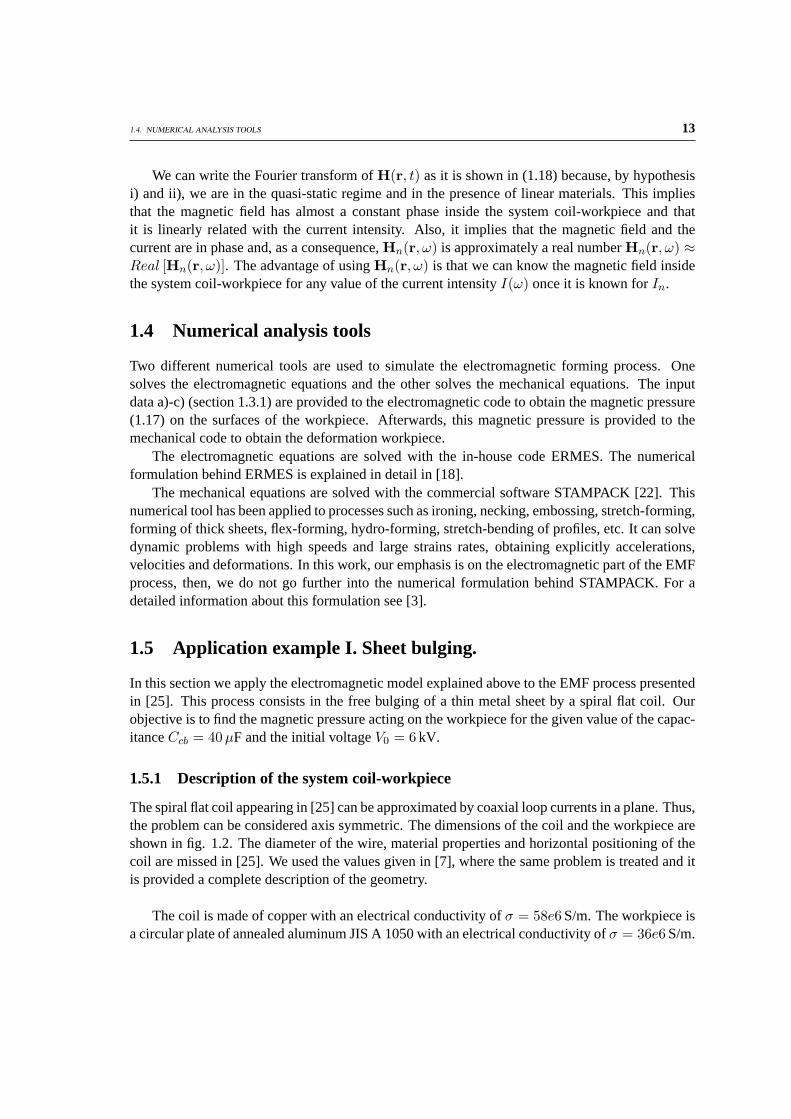
We employed the geometry shown in fig. 1.3 to compute the electromagnetic fields withERMES. The geometry is a truncated portion of a sphere with an angle of 20o. We drive theproblem with a current densityJ uniformly distributed in the volume of the coil wires. In thecolored surfaces of fig. 1.3 we imposed the regularized perfect electric conductor (PEC) boundaryconditions (see chapter 3)

∇ · (εE) = 0,

n×E = 0.(1.22)

It is not necessary to impose more boundary condition if we apply in all the FEM nodes of thedomain a change of coordinates from cartesian(Ex, Ey, Ez) to axis symmetric around the Y axis(Eρ, Eϕ, Ey). That is, at the same time we are building the matrix, we enforce at each node of the

1.5. APPLICATION EXAMPLE I. SHEET BULGING. 15

FEM mesh the following Eρ

Eϕ

Ey

=

x/ρ 0 z/ρ−z/ρ 0 x/ρ

0 1 0

Ex

Ey

Ez

(1.23)

wherex andz are the cartesian coordinates of the node andρ =√

x2 + z2. We preserve thesymmetry of the final FEM matrix applying (1.23) and its transpose as it is explained in [2].

The advantage of using (1.23) is thatEρ = 0 andEy = 0 in axis symmetric problems. Thisfact reduces by a factor of three the size of the final matrix and also the time required to solveit. Therefore, we can improved noticeably the computational performance of ERMES in axissymmetric problems with a simple modification of its matrix building procedure. In a desktopcomputer with a CPU Intel Core 2 Quad Q9300 at 2.5 GHz and the operative system MicrosoftWindows XP, ERMES requires less than 30 s and less than 500 MB of memory RAM to solveeach frequency.

Figure 1.3: Geometry used in ERMES to compute the electromagnetic fields in the free bulging process ofa thin metal sheet by a spiral flat coil.


1.5.3 Intensity through the RLC circuit

Once the initial geometry of system coil-workpiece is properly characterized, we have to find theintensityI(t) flowing through the RLC circuit. As it is mentioned in section 1.3.4, if we wantto know I(t) we have to calculate first the frequencyω0. This frequencyω0 is the solution ofequation (1.9) withCcb = 40µF. We solved (1.9) using the following iterative procedure:

1) We replace inC0(ω) the frequency which satisfiesδ = τ , whereτ is the thickness of theworkpiece andδ is the skin depth

δ =√

1πνµσ

. (1.24)

2) We compareC0(ω) with Ccb. If C0(ω) > Ccb then we must increase the value ofω. IfC0(ω) < Ccb then we must decrease the value ofω. If C0(ω) = Ccb then we have foundthe solutionω0.

3) If the solution is not achieved then we replace inC0(ω) the new incremented/decrementedvalue ofω and go to step 2). The procedure is repeated until the solution is achieved.

In fig. 1.4 is shown the capacitanceC0 as a function of the frequencyν and the solutionν0 =16.35 kHz for the given capacitanceCcb = 40 µF. We have choose an initial frequency satisfyingδ = τ because we have observed in the literature that the typical frequencies employed in EMFlay in the interval

0.5 <δ

τ< 1.5. (1.25)

In the present case, we have that the skin depth isδ = 1.3 τ .As it is indicated in equation (1.10), we need to knowL0(ω) andR0(ω) to calculateC0(ω).

These functions are defined in (1.3) and they represent the total inductance and the total resistanceof the RLC circuit of fig. 1.1. We assume that the given valuesLcb + Lcon = 2.0 µH andRcb + Rcon = 25.5 mΩ do not change with the frequency. On the other hand,Lwp andRwp arefrequency dependant and they have to be calculated with the help of (1.1) and (1.2). In the volumeof the coil, equation (1.2) is replaced by

Rcw(ω) =1|In|2

∫υ

|J|2

σdυ (1.26)

whereJ is the imposed current density andσ is the conductivity of the coil. We recall that if wewant to obtain a volume integral for all the space then we must multiply by 18 (=360o/20o) anyvolume integral calculated in the portion of truncated sphere of fig. 1.3. The values of the totalinductanceL0 and the total resistanceR0 as a function of the frequencyν are shown in fig. 1.5and in fig. 1.6.

If we substitute in equation (1.6) the calculated values ofω0 = 2πν0, L0(ω0) = 2.35 µHandR0(ω0) = 38.1 mΩ and the given values ofCcb andV0 then we obtain the intensityI(t)flowing through the coil. In fig. 1.7 we compare the intensity calculated in [25] with the intensitycalculated in this work.


Figure 1.4: CapacitanceC0 as a function of the frequencyν for the un-deformed workpiece placed inits initial position. The functionC0(ν) is obtained from equation (1.10). If the capacitor bank has aCcb = 40 µF the oscillation frequency of the RLC circuit isν0 = 16.35 kHz.

Figure 1.5: Total inductanceL0 = Lcb + Lcon + Lcw as a function of the frequencyν for the un-deformedworkpiece placed in its initial position. The inductance of the system coil-workpieceLcw is calculated withthe equation (1.1). The value ofLcw varies from0.86 µH at the lower frequencies to0.35 µH at the higherfrequencies. We assumed that the inductance of the exterior circuitLcb + Lcon = 2.0 µH remains constantin this frequency band.


Figure 1.6: Total resistanceR0 = Rcb + Rcon + Rcw as a function of the frequencyν for the un-deformedworkpiece placed in its initial position. The resistance of the system coil-workpieceRcw is calculated withequation (1.2) in the volume of the workpiece and with equation (1.26) in the volume of the coil. The valueof Rcw varies from8.4 mΩ at the lower frequencies to13.2 mΩ at the higher frequencies. We assumed thatthe resistance of the exterior circuitRcb + Rcon = 25.5 mΩ remains constant in this frequency band.

Figure 1.7: Intensity calculated in Takatsu et al. [25] compared with the intensity calculated in this work.We have graphed expression (1.6) withV0 = 6 kV, Ccb = 40 µF, ν0 = 16.35 kHz, ω0 = 2πν0, L0 =2.35 µH andR0 = 38.1 mΩ.


1.5.4 Magnetic pressure on the workpiece

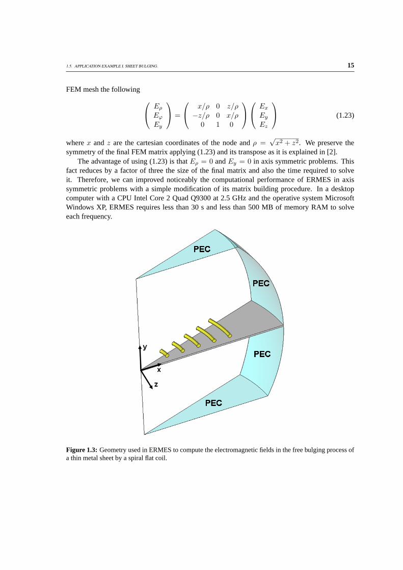
If we want to calculate the magnetic pressure (1.17) acting on the workpiece then we need thefieldsH(r0, t) andH(rτ , t), wherer0 is located on the surface of the workpiece nearest to the coil(S0) andrτ is located on the surface of the workpiece farthest to the coil (Sτ ). The fieldsH(r0, t)andH(rτ , t) are obtained from (1.18) with the Fourier transform ofI(t) and the magnetic fieldsper unit intensityHn(r0, ω) andHn(rτ , ω). In fig. 1.8 are shown|Hn(r0, ω)| and|Hn(rτ , ω))|as a function of the frequencyν. In fig. 1.9 are shown|Hn(r0, ω0) I(ω)|, |Hn(r0, ω)) I(ω)| and|Hn(rτ , ω)) I(ω)| as a function of the frequencyν. It can be shown (see fig. 1.9) that, in this EMFprocess, we have

Hn(r0, ω0) I(ω) ≈ Hn(r0, ω) I(ω),|Hn(r0, ω0) I(ω)| |Hn(rτ , ω) I(ω)|.

(1.27)

If we use (1.27) in (1.18) and (1.17) then we can write the magnetic pressureP (r0, t) as

P (r0, t) =12

µ0|Hn(r0, ω0) I(t)|2. (1.28)

This simplification of (1.17), which is possible when (1.27) is accomplished, is very useful in asequential coupling strategy. This is so because, in the next calls to the electromagnetic model, wewill only need to find the magnetic field for one frequency, which makes the computations moreefficient.

Figure 1.8: Modulus of the magnetic fields per unit intensity|Hn(r0, ω)| and|Hn(rτ , ω)| as a function ofthe frequencyν. The pointr0 is located onS0. The pointrτ is located onSτ , on the opposite side of wherer0 is placed.


Figure 1.9: Modulus of the magnetic fields|Hn(r0, ω0) I(ω)|, |Hn(r0, ω) I(ω)| and |Hn(rτ , ω) I(ω)|as a function of the frequencyν. The constantHn(r0, ω0) is the magnetic field per unit intensity at thefrequencyω0 in the pointr0. The pointr0 is located onS0. The functionI(ω) is the Fourier transformof the intensityI(t). The analytical expression ofI(ω) is given by (1.20). The functionHn(r0, ω) is themagnetic field per unit intensity at the pointr0. The functionHn(rτ , ω) is the magnetic field per unitintensity at the pointrτ . The pointrτ is located onSτ , on the opposite side of wherer0 is placed. In thisgraph we can see that|Hn(r0, ω0) I(ω)| ≈ |Hn(r0, ω) I(ω)| and|Hn(r0, ω0) I(ω)| |Hn(rτ , ω) I(ω)|.

In fig. 1.10 is shown the total magnetic force acting on the workpiece as a function of time.The total magnetic force is the integral of the function (1.28) over the whole surfaceS0. Wecomputed the total force using (1.28) withHn(r0, ω0) andI(t) calculated for the un-deformedworkpiece placed in its initial position.

In fig. 1.11 is shown the radial distribution of the magnetic pressure (1.28) when the coilcurrent reaches its maximumImax = 21.83 kA at t = 14.5 µs. In fig. 1.11 is also shown themagnetic pressure obtained in [25] when the coil current calculated there reaches its maximum att = 15.4 µs. In fig. 1.11 we see that, apart from a difference in the positioning of the coil, thereis a difference in the magnitude of the magnetic pressure. The same difference is also observedin [21, 20], where this EMF process is simulated using two different approaches. One is basedon FDTD (Finite Difference Time Domain) and the other on FEM (Finite Element Method). Inthe FDTD approach they used a similar procedure to that employed in [25]. In the FEM approachthey used the freeware software FEMM4.0 [6]. In fig. 1.12 and fig. 1.13 we show the componentsof the magnetic flux densityBρ andBy calculated with FEMM4.0, FDTD and ERMES when thecoil current isI = 20.81 kA. In these figures we see that the results given by both FEM codes aresimilar between them but different from the results given by the FDTD method.


Figure 1.10: Total magnetic force calculated in Takatsu et al. [25] compared with the total magnetic forcecalculated in this work.

Figure 1.11: Radial distribution of the magnetic pressure calculated in Takatsu et al. [25] when the coilcurrent reaches its maximum (t = 15.4 µs) compared with the radial distribution of the magnetic pressurecalculated in this work (Imax = 21.83 kA at t = 14.5 µs).


Figure 1.12: Radial component of the magnetic flux density calculated in [21] with FEM (FEMM4.0)and FDTD compared with the radial component of the magnetic flux density calculated in this work withERMES.

Figure 1.13: Axial component of the magnetic flux density calculated in [21] with FEM (FEMM4.0)and FDTD compared with the axial component of the magnetic flux density calculated in this work withERMES.


The differences between the FDTD and the FEM approaches can be attributed to the use of acoarse mesh in the FDTD method. To show this, we solved a problem similar to the one appearingin this section (see fig. 1.2) but with a fixed workpiece of thicknessτ = 3.0 mm, gap distanceh = 2.9 mm and initial voltageV0 = 2 kV. We calculated in this set-up the radial component ofthe magnetic flux densityBρ. Then, we compared our results with the simulations performed in[20] for different FDTD mesh sizes and also with the measurements of [25] (see fig. 1.14).

In fig. 1.14 we see that when the FDTD mesh is coarse (6 elements along the thickness ofthe sheet) the results of the FDTD simulations are in good agreement with the measurements butthey are different from the results obtained with ERMES. On the hand, if we improve the FDTDmesh to 20 elements along the thickness of the sheet, the results of the FDTD simulations aresimilar to the results obtained with ERMES but they are different from the measurements. Thisunusual behavior can be explained if we consider thatRcon andLcon are undervalued. If we add,for instance, only 1 meter of 16 AWG copper wire (R1m = 13.2 mΩ, L1m = 1.5 µH [8]) to thetotal resistance and the total inductance of the RLC circuit then, the results obtained with ERMES,and with the improved FDTD mesh, are in agreement with the measurements and also with thefact that improving the mesh must improve the results.

Figure 1.14: Radial component of the magnetic flux densityBρ for the coil of fig. 1.2 with a fixed work-piece of thicknessτ = 3.0 mm, gap distanceh = 2.9 mm and initial voltageV0 = 2 kV. Measurements arefrom [25]. FDTD (6x110) represents the simulations performed in [20] with a FDTD mesh of 6 elementsalong the thickness of the sheet and 110 elements along the radial direction. FDTD (20x110) represents thesimulations performed in [20] with a FDTD mesh of 20 elements along the thickness of the sheet and 110elements along the radial direction. ERMES represents the simulations performed in this work. ERMES(+1m wire) represents the simulations performed in this work adding the DC resistance and the inductanceof 1 meter of 16 AWG copper wire (R1m = 13.2 mΩ, L1m = 1.5 µH [8]) to the total inductance and thetotal resistance of the RLC circuit.


1.5.5 Deflection of the workpiece

We introduced in STAMPACK the magnetic pressure calculated in section 1.5.4 to obtain the de-flection of the metal sheet. STAMPACK interprets the magnetic pressure as a mechanical pressurewhich deforms the workpiece. The results are shown in fig. 1.15.

In STAMPACK is not available the mechanical model used in [25]. Therefore, we had to adaptthe parameters of the available model to reproduce the behavior of the material used in [25]. Weconsidered the workpiece as an aluminium alloy with a Young’s modulusE = 69 GPa, densityρ = 2700 Kg/m3 and Poisson’s ratioν = 0.33. STAMPACK used the Voce hardening law

σcs = σy0 + (σm − σy0)(1− e−nεps

), (1.29)

whereσcs is the Cauchy stress,σy0 = 34.9 MPa is the yielding tensile strength,σm = 128.8 MPais the ultimate tensile strength,n = 12.0 is the isotropic hardening parameter andεps is the ef-fective plastic deformation. STAMPACK also used a damping proportional to the nodal velocity(Fi = −ηi vi) with ηi = 2αMi, beingα = 138.6 andMi the lumped mass at the i-th node. Theconstant parameters of the mechanical model were obtained introducing in STAMPACK the mag-netic pressure calculated in [25]. Then, we adjusted the parameters until achieve with STAMPACKthe same deflection of the disk as the one measured in [25].

Figure 1.15: Deflection of the workpiece at the positionsx = 0 mm andx = 20 mm as a function of time.The results of this work are compared with the measurements of Takatsu et al. [25].

1.6. APPLICATION EXAMPLE II. TUBE BULGING. 25

1.6 Application example II. Tube bulging.

In this section we apply the electromagnetic model of section 1.3 to the EMF process presentedin [28]. This process consists in the expansion of a cylindrical tube by a solenoidal coil. In [28]is analyzed the tube bulging process under different working conditions but, here, our objective isto find the magnetic pressure acting on the workpiece when the capacitance isCcb = 160 µF, thecoil length is` = 200 mm and the initial charging energy isU0 = 2 kJ.

1.6.1 Description of the system coil-workpiece

We take the geometrical description of the solenoidal coil and the tubular workpiece from [28].The coil is approximated by coaxial loop currents, concentric with the workpiece and placed insideit. Thus, the problem is considered axis symmetric.

The coil is made ofd = 2.0 mm diameter copper wire. The outer diameter of the coil isDc = 37.0 mm. The separation between each loop isp = 3.0 mm. The length of the coil isapproximately = 200 mm and the number of turns isN = 68. We assume an electrical conduc-tivity for copper ofσ = 58e6 S/m.

The workpiece is a cylindrical tube made of annealed aluminum A1050TD with an outerdiameterDwp = 40.0 mm and a thickness ofτ = 1.0 mm. We assume an electrical conductivityfor the workpiece ofσ = 36e6 S/m. We also assume thatε = ε0 andµ = µ0 for workpiece andcoil.

In [28] is said thatLcb+Lcon andRcb+Rcon are less than1.0 µH and2.0 mΩ respectively. But,in [16], where it is used an EMF set-up similar to that used in [28], it is reached to the conclusionthat these quantities underestimate the inductance and the resistance of the wires connecting thecapacitor bank with the coil. In [16] is found thatLcb+Lcon = 2.5 µH andRcb+Rcon = 15.0 mΩare more realistic values. In this work we employ theLcb + Lcon andRcb + Rcon given in [16].

Figure 1.16: Geometry used in ERMES to compute the electromagnetic fields of the tube bulging processanalyzed in [28].


1.6.2 Finite element model

The FEM model used for the tube bulging process is similar to that described in section 1.5.2. Wecomputed the fieldsE(r, ω) andH(r, ω) in the geometry of fig. 1.16. The geometry represents atruncated portion of one turn of the coil with an angle of 20o. The problem is driven by a currentdensity uniformly distributed in the volume of the wire. We applied the PEC boundary condition(1.22) in the colored surface of fig. 1.16. We imposed the change of coordinates explained insection 1.5.2 at each node of the FEM mesh. One of the advantages of using the geometry of fig.1.16 is that we can obtainLwp andRwp for any coil length. We only need to multiply the integrals(1.1) and (1.2) performed in the volume of fig. 1.16 byN · (360o/20o), whereN is the number ofturns of the coil.

1.6.3 Intensity through the RLC circuit

We follow the steps given in section 1.5.3 to compute the intensity flowing trough the coil of length` = 200 mm (N = 68 turns) when the capacitance isCcb = 160µF and the initial charging energyis U0 = 2 kJ. We found thatν0 = 4.6 kHz, V0 = 5 kV, L0 = 6.9 µH andR0 = 101.1 mΩ, beingL0 = Lcb + Lcon + Lcw andR0 = Rcb + Rcon + Rcw.

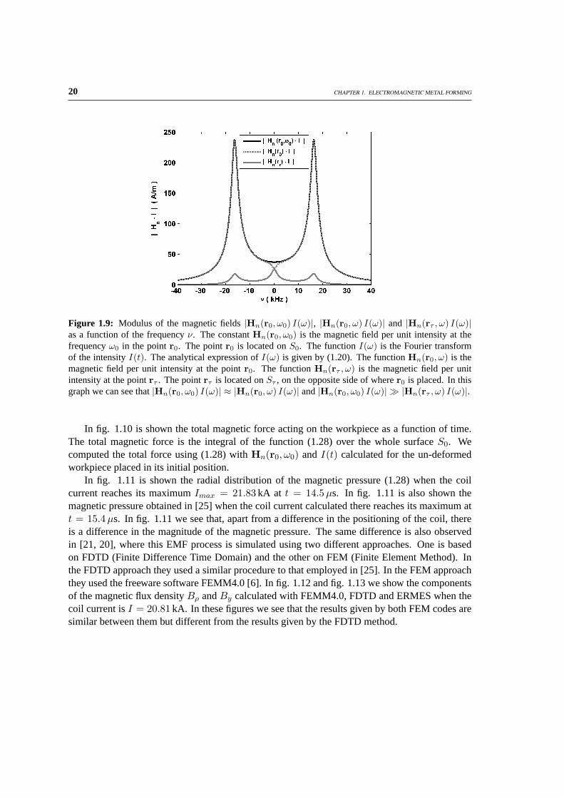
In [28] is measured the maximum current intensity for several coil lengths and capacitancesCcb when the initial charging energy isU0 = 1 kJ. In fig. 1.17 we compare these measurementswith the results of this work.

Figure 1.17: Maximum current intensity for several coil lengths and capacitancesCcb. The initial chargingenergy isU0 = 1 kJ in all the cases. The measurements from [28] are compared with the results of thiswork.

1.6. APPLICATION EXAMPLE II. TUBE BULGING. 27

1.6.4 Magnetic pressure on the workpiece

In fig. 1.18 we show the modulus of the magnetic fields|Hn(r0, ω0) I(ω)|, |Hn(r0, ω) I(ω)| and|Hn(rτ , ω) I(ω)| as a function of the frequencyν, where the notation used here is the same asin section 1.5.4. In this case we can not apply the approximations (1.27) and (1.28) and we mustemploy the equations (1.18) and (1.17) to calculate the magnetic pressure acting on the workpiece.

In fig. 1.19 we show the magnetic pressure calculated in this work compared with the magneticpressure calculated in [28]. We had to average the magnetic pressure over the surfaces of theworkpiece to compare our results with those provided by [28].

The differences shown in fig. 1.19 can be attributed to the features of each electromagneticmodel. In [28] is considered the movement of the workpiece, assumed a uniform current densityalong all the the length of the coil and an exponential decay of the magnetic field from the innersurface to the outer surface of the metallic tube. On the other hand, we neglected the workpiecedeformation, considered a more realistic coil geometry and calculated numerically the magneticfield on the surfaces of the metallic tube.

Figure 1.18: Modulus of the magnetic fields|Hn(r0, ω0) I(ω)|, |Hn(r0, ω) I(ω)| and|Hn(rτ , ω) I(ω)| asa function of the frequencyν.

1.6.5 Deflection of the workpiece

We calculated the expansion of the workpiece using the mechanical model explained in section1.5.5. The material properties and constant parameters are the same as in section 1.5.5 except forthe damping coefficientα, which now isα = 693.1.

The parameters of the mechanical model were obtained by introducing in STAMPACK themagnetic pressure calculated in [28]. Then, we adjusted the parameters until reproduce the form-ing velocity given in [28].


Figure 1.19: Magnetic pressure calculated by Zhang et al. [28] compared with the magnetic pressurecalculated in this work.

In fig. 1.20 we compare the deflection of the workpiece deduced from [28] with the deflectionof the workpiece calculated in this work. In [28] is not provided the deflection of the workpiece,we obtained it by integrating in time the forming velocity facilitated there.

Figure 1.20: Deflection of the workpiece as a function of time. The results of Zhang et al. [28] arecompared with the results of this work.

1.7. OPTIMUM FREQUENCY AND OPTIMUM CAPACITANCE 29

1.7 Optimum frequency and optimum capacitance

The frequency at which the discharge current oscillates is a key parameter in the design of anelectromagnetic forming system. In [9, 28, 10] it is shown that, for a fixed energyU0 and a givenset of capacitor bank, connectors, coil and workpiece, there exist a frequencyνop at which themaximum deformation of the workpiece is achieved. The use of this optimum frequency savesenergy and prevents the premature wearing of the coil.

The frequency of the dischargeν is controlled by the capacitanceCcb for a given set of ca-pacitor bank, connectors, coil and workpiece. The relationship betweenCcb andν is describedby equations (1.7) and (1.10). Therefore, the search for the optimum frequencyνop is equivalentto the search for the optimum capacitanceCop. Usually, in EMF, there is only a discrete set ofcapacitancesCcb available in the capacitor bank. Then, once we have determinedCop we mustsearch for the closest availableCcb. In this work, we will refer indistinctly to the available valueor to the theoretical value as the optimum capacitanceCop.

The optimum capacitance can be obtained computing the deformation of the workpiece for theavailableCcb using the same initial charging energyU0 in all the numerical simulations. There-after, we select the capacitanceCcb which produces the maximum deformation. This is the ap-proach followed in [9, 28, 10]. We can reduce the number of electro-mechanical simulations if wemake an initial estimationCig close to the optimum valueCop. In fact, if Cig is close enough, wecan findCop with only three simulations. For instance, suppose thatCig falls between two avail-able capacitancesC1 andC2, beingC1 < C2. We make two electro-mechanical simulations andobtain that the deflections of the workpiece satisfyh1 < h2. Afterwards, we take a capacitanceC3 which is the lower value available such asC2 < C3. If we compute thath2 > h3 thenC2 is theoptimum capacitance. In this case, we have required only three electro-mechanical simulations.On the other hand, ifh2 < h3, we must keep on testing with successiveCn until find an suchashn > hn+1. When this happens, we have thatCn is the optimum capacitance andn + 1 thenumber of electro-mechanical simulations. Therefore, the betterCig is the lessn + 1 is.

The simplest way to find an initial guess is derived from expression (1.25). As it is mentionedin section 1.5.3, we have observed in the literature that the typical frequencies employed in EMFlay in the interval (1.25). Therefore, we can consider an initial estimationνig as the frequencywhich satisfiesδ = τ .

We can improve the initial guess if we have prior knowledge about the workpiece. For instance,in [9], it is stated that the optimum frequency for the compression of a tube of thicknessτ = 2 mmmade of aluminium AA3003 satisfiesδ = 0.66 τ . If we are going to use the same workpiece ina different EMF process (different coil or capacitor bank) we can try the frequency which satisfyδ = 0.66 τ as the initial guess. The same can be applied to the workpiece used in [28], where itis found that the optimum frequency for the expansion of a tube of thicknessτ = 1 mm made ofaluminium A1050TD satisfiesδ = 0.9 τ .

In the case we do not posses any prior knowledge about workpiece we propose a method tofind νig. The idea is to look for the frequency which produces the maximum momentumP in thefirst n semi-periods, where a semi-period is half a periodT/2 = 1/2ν. That is, we look for the


frequency which makes maximum the quantity

∆Pn =∫ n

2ν

0Ftot · dt, (1.30)

whereFtot is the total magnetic force acting on the workpiece and∆Pn is the momentum pro-duced by this force in the firstn semi-periods. The numbern depends on the application and weobtained the best results with the minimum natural number which accomplish

n ≥ 4L0ν∞R0

, (1.31)

whereL0 andR0 are the inductance and the resistance defined in section 1.3.3 andν∞ is thefrequency which makes maximum the quantity∆P∞. The quantity∆P∞ is obtained whenn →∞ in (1.30). L0 andR0 are evaluated at the frequencyν∞. The expression (1.31) comes fromreordering(n/2ν) ≥ (1/γ0), whereγ0 is defined in (1.8), and it represents the minimum numberof semi-periods required to release more than 80% of the total momentum∆P∞.

In summary, we first locate the frequencyν∞ which makes maximum the quantity∆P∞.Second, we computen with (1.31) atν∞. Finally, νig is the frequency which makes maximum∆Pn, beingn the natural number calculated in the second step. All this process is performedneglecting the workpiece deformation. We do not require any additional simulation. We are usingthe data obtained in the initial frequency sweep of our electromagnetic model. It takes only a fewseconds to compute all the integrals and obtainνig. In the next section we apply this method totwo particular examples.

1.8 Optimum capacitance estimation

In this section we are going to obtain an initial guessCig for the tube bulging process analyzedin [28] and for the tube compression process analyzed in [9]. We apply the method proposed insection 1.7 to calculateCig.

1.8.1 Tube bulging

In [28] is analyzed the expansion of a tube by a solenoidal coil under different working conditions.They used several coils with lengths` = 100, 200, 300, 400,500mm. They computed foreach coil the bulge height with the capacitance varying fromCcb = 20 µF to Ccb = 1600 µF.They obtained the optimum capacitanceCop for each coil length and concluded that the optimumfrequency satisfyδ = 0.9 τ in all the cases.

We analyzed this problem with the geometry, material properties and FEM model detailed insection 1.6. We found that the number defined in (1.31) isn = 2 in all the cases. Then, theinitial guessCig is the capacitance which makes maximum the quantity∆P2 defined in (1.30). Infig. 1.21 we show the momentum∆P2 as a function of the capacitanceCcb for the coil lengths` = 200, 300, 400,500mm and the initial charging energyU0 = 2 kJ. In Table 1.1 we show thevalues ofCig compared with the optimum capacitancesCop calculated in [28].

1.8. OPTIMUM CAPACITANCE ESTIMATION 31

In [28] is also analyzed a coil with = 100 mm andU0 = 1 kJ. They measure the bulgeheight for the capacitancesCcb = 24, 50, 100, 200, 400, 800,1600µF and they found that themaximum height was inCcb = 200µF. They also calculated numerically the optimum capacitanceand they obtained a value ofCop = 310 µF. We calculated the initial guess with the method ofsection 1.7 and we found thatCig = 296µF.

Figure 1.21: Momentum∆P2 as a function of the capacitanceCcb for several coil lengths. The initialcharging energy isU0 = 2 kJ in all the cases. The initial guessCig is the capacitance which makes maxi-mum the quantity∆P2. The values ofCig are shown in Table 1.1.

` (mm) Cop (µF) Cig (µF)

200 160 161

300 100 108

400 70 83

500 40 67

Table 1.1: Optimum capacitance (Cop) and initial guess (Cig) for different coil lengths ().

1.8.2 Tube compression

In [9] is analyzed the compression of a tube by a solenoidal coil for the capacitancesCcb = 60,120, 240, 360, 480, 600, 702, 720, 840, 960, 1080,1800µF and the initial charging energyU0 = 2.02 kJ. They computed the radial displacement of the walls of the tube and they found thatthe maximum displacement occurs whenCop = 840µF, νop = 4.97 kHz andδ = 0.66 τ .


We analyzed numerically this problem with the geometry of fig. 1.22. The geometry representshalf of the coil and the workpiece placed inside a truncated portion of a semi-sphere with an angleof 20o. The FEM model used here is similar to that described in sections 1.5.2 and 1.6.2.

The workpiece is made of the aluminium alloy AA3003. The electrical conductivity isσ =29.4e6 S/m. The outer diameter of the workpiece isDwp = 50.0 mm. Its thickness isτ = 2 mmand its length is = 100.0 mm.

The solenoidal coil is approximated by coaxial loop currents, concentric with the workpieceand placed outside it. The coil is made of copper with a conductivity ofσ = 58e6 S/m. Theinner diameter of the coil isDc = 56.0 mm. The separation between each loop isp = 6.25 mm.The length of the coil is = 100 mm and the number of turns isN = 17. The dimensions ofthe coil wires are not provided in [9]. We assumed a thickness of4xc = 5 mm and a height of4yc = 3 mm for each coil wire.

In [9] is assumed thatR0 = Rcb + Rcon + Rcw = 13.03 mΩ andL0 = Lcb + Lcon + Lcw =1.22 µH for all the frequencies. Therefore, for comparison purposes, we assumed the same.

We found that the maximum of∆P∞ was inν∞ = 13 kHz. If we substituteν∞, L0 andR0

in (1.31), we have thatn = 5. Then,Cig is the capacitance which makes maximum the quantity∆P5. In fig. 1.23 we show the momentum∆P5 as a function of the capacitanceCcb. Themaximum is atCig = 805µF, νig = 5 kHz andδ = 0.66 τ .

Figure 1.22: Geometry used in ERMES to compute the electromagnetic fields of the tube compressionprocess analyzed in [9].

1.9. SUMMARY 33

Figure 1.23: Momentum∆P5 as a function of the capacitanceCcb. The initial guessCig is the capacitancewhich makes maximum the quantity∆P5. The value of the initial guess isCig = 805µF.

1.9 Summary

In this report we have presented a numerical model for the simulation of electromagnetic formingprocesses. This method is computationally efficient because it only requires to solve the time-harmonic Maxwell equations for a few frequencies to have completely characterized the EMFsystem. The approach can be very useful for estimating the order of magnitude of the parametersof an EMF process, for experimentation on modeling conditions or for modeling complex geome-tries. Moreover, it can be easily included in a sequential coupling strategy without the worry ofnumerical instabilities. The method provides an explicit relation between the capacitance of the ca-pacitor bank and the frequency of the discharge. This allow us to estimate the optimum frequencyand capacitance at which it is attained the maximum workpiece deformation for a given initialenergy and a given set of coil and workpiece. Also, it offers an alternative to the more extendedtime domain methods and a new insight into the physics of EMF. Finally, we have shown that thenumerical results provided by this method exhibit a good correlation with the measurements andwith the theoretical developments of other authors.

Bibliography

[1] G. Bartels, W. Schaetzing, H.-P. Scheibe, and M. Leone. Simulation models of the electro-magnetic forming process.Acta Physica Polonica A, 115:1128–1129, 2009.

[2] W. E. Boyse, D. R. Lynch, K. D. Paulsen, and G. N. Minerbo. Nodal-based finite-element modeling of Maxwell’s equations.IEEE Transactions on Antennas and Propagation,40:642–651, 1992.

[3] P. Cendoya, E. Onate, and J. Miquel. Nuevos elementos finitos para el analisis dinamicoelastoplastico no lineal de estructuras laminares. Technical report, International Center forNumerical Methods in Engineering (CIMNE), ref.: M-36, 1997.

[4] M. S. Dehra.High Velocity Formability And Factors Affecting It. PhD thesis, The Ohio StateUniversity, 2006.

[5] A. El-Azab, M. Garnich, and A. Kapoor. Modeling of the electromagnetic forming ofsheet metals: state-of-the-art and future needs.Journal of Materials Processing Technology,142:744–754, 2003.

[6] FEMM. Finite element method magnetics.David Meeker, USA. [Online]. Available:http://www.femm.info/wiki/HomePage, 2010.

[7] G. K. Fenton and G. S. Daehn. Modelling of the electromagnetically formed sheet metal.Journal of Materials Processing Technology, 75:6–16, 1998.

[8] F. W. Grover.Inductance Calculations. Dover Publications, 2004.

[9] Y. U. Haiping and L. I. Chunfeng. Effects of current frequency on electromagnetic tubecompression.Journal of Materials Processing Technology, 209:1053–1059, 2009.

[10] J. Jablonski and R. Winkler. Analysis of the electromagnetic forming process.InternationalJournal of Mechanical Sciences, 20:315–325, 1978.

[11] J. D. Jackson.Classical Electrodynamics. John Wiley & Sons, Inc., 3rd edition, 1999.

[12] M. Kleiner, A. Brosius, H. Blum, F.-T. Suttmeier, M. Stiemer, B. Svendsen, J. Unger, andS. Reese. Benchmark simulation for coupled electromagnetic-mechanical metal forming pro-cesses.Production Engineering and Development, 11:85–90, 2004.

35

36 BIBLIOGRAPHY

[13] A. G. Mamalis, D. E. Manolakos, A. G. Kladas, and A. K. Koumoutsos. Physical principlesof electromagnetic forming process: a constitutive finite element model.Journal of MaterialsProcessing Technology, 161:294–299, 2005.

[14] A. G. Mamalis, D. E. Manolakos, A. G. Kladas, and A. K. Koumoutsos. Electromagneticforming tools and processing conditions: numerical simulation.Materials and Manufactur-ing Processes, 21:411–423, 2006.

[15] T. E. Manea, M. D. Verweij, and H. Blok. The importance of the velocity term in the electro-magnetic forming process.The 27th General Assembly of the International Union of RadioScience (URSI 2002), Maastricht, The Netherlands, 17-24 August, 2002.

[16] T. E. Motoasca.Electrodynamics in Deformable Solids for Electromagnetic Forming. PhDthesis, Delft University of Technology, 2003.

[17] D.A. Oliveira, M.J. Worswick, M. Finn, and D. Newmanc. Electromagnetic forming of alu-minum alloy sheet: Free-form and cavity fill experiments and model.Journal of MaterialsProcessing Technology, 170:350–362, 2005.

[18] R. Otin. Regularized Maxwell equations and nodal finite elements for electromagnetic fieldcomputations.Electromagnetics, 30:190–204, 2010.

[19] J. Shang.Electromagnetically Assisted Sheet Metal Stamping. PhD thesis, The Ohio StateUniversity, 2006.

[20] M. A. Siddiqui.Numerical Modelling And Simulation Of Electromagnetic Forming Process.PhD thesis, University of Strasbourg, 2009.

[21] M. A. Siddiqui, J. P. M. Correia, S. Ahzi, and S. Belouettar. A numerical model to simulateelectromagnetic sheet metal forming process.International Journal of Material Forming,1:1387–1390, 2008.

[22] STAMPACK. A general finite element system for sheet stamping and forming problems.Quantech ATZ, Barcelona, Spain. [Online]. Available: http://www.quantech.es, 2010.

[23] J. A. Stratton.Electromagnetic Theory. McGraw-Hill, 1941.

[24] B. Svendsen and T. Chanda. Continuum thermodynamic formulation of models for electro-magnetic thermoinelastic solids with application in electromagnetic metal forming.Contin-uum Mechanics and Thermodynamics, 17:1–16, 2005.

[25] N. Takatsu, M. Kato, K. Sato, and T. Tobe. High-speed forming of metal sheets by electro-magnetic force.The Japan Society of Mechanical Engineers International Journal, 31:142–148, 1988.

[26] I. Ulacia, I. Hurtado, J. Imbert, M. J. Worswick, and P. L’Eplattenier. Influence of the cou-pling strategy in the numerical simulation of electromagnetic sheet metal forming.The 10thInternational LS-DYNA Users Conference, Dearborn, Michigan USA, June 8-10, 2008.

BIBLIOGRAPHY 37

[27] J. Unger, M. Stiemer, M. Schwarze, B. Svendsen, H. Blum, and S. Reese. Strategies for 3Dsimulation of electromagnetic forming processes.Journal of Materials Processing Technol-ogy, 199:341–362, 2008.

[28] H. Zhang, M. Murata, and H. Suzuki. Effects of various working conditions on tube bulgingby electromagnetic forming.Journal of Materials Processing Technology, 48:113–121,1995.

electromagnetic metal forming -...

Documents