Thesis Proposal

Electromagnetic Ion Cyclotron (EMIC) Waves for Radiation Belt Remediation Applications

Maria de Soria-Santacruz Pich

Ph.D Candidate - Aero/Astro Department

Massachusetts Institute of Technology

Submitted: March 26th, 2012

Defense: April 9th, 2012

Committee: Manuel Martinez-Sanchez (supervisor), Gregory Ginet, David Miller, Jeffrey Hoffman

and Kerri Cahoy

Abstract

The high energy particles of the Van Allen belts coming from cosmic rays, solar storms, high altitude nuclearexplosions (HANEs) and other processes represent a significant danger to humans and spacecraft operating inthose regions, as well as an obstacle to exploration and development of space technologies. The "RadiationBelt Remediation" (RBR) concept has been proposed as a way to solve this problem through ULF/VLFtransmissions in the magnetosphere, which will create a pitch-angle scattering of these energetic particles. Aportion of the particles would then fall into their loss cone, lowering the altitude of their mirror point to a levelwhere they are absorbed by the atmosphere.

The possible utilization of Whistler waves for precipitation of high-energy trapped electrons has been studiedextensively [54], and a space test of a linear antenna for this purpose is in preparation [39]. The lower frequencyEMIC band has also been studied in the context of electron precipitation [8], but much less work has beendevoted to the use of the left-hand polarized branch of EMIC waves for ion precipitation. My thesis focuseson four interconnected research efforts in this direction, which are (1) the radiation of EMIC waves from aspaceborne antenna, (2) their propagation along the Van Allen belts, (3) their interaction with the high-energyparticles and (4) the characterization in terms of power, frequency, voltage and current of the RBR transmittercapable of significantly reduce the energetic radiation in the belts. This proposal summarizes the formulationand methodology required to develop these coupled studies as well as the results obtained so far.

The radiation of this frequency band is a broad unexplored territory that should be addressed given its potentialpractical importance. In my thesis, I will propose solutions to this problem and determine their feasibility.The sheath around a space-based RBR antenna is very thick, and so its capacitance is almost the vacuumcapacitance, which is nearly independent of the frequency and proportional to the transmitter length. Theassociated reactance is extremely high for the EMIC band to the point that it is not possible to use an electricdipole to radiate these waves without the help of any other device. On the other hand, in terms of the radiationresistance, a short antenna would be ideal, because the relevant wavelengths (those near the resonance cone)are indeed very short; unfortunately, short antennas suffer the most from the small capacitance problem,although even a multi-km antenna would have too much reactance at the EMIC regime. In my thesis I willdiscuss two innovative ways to emit these waves; the first option involves plasma contactors at both ends of alinear dipole, thus avoiding oscillatory charge accumulation. The second case under consideration consists ofa magnetic dipole working as an EMIC transmitter. Once the emitter’s radiation pattern has been estimated,the propagation of the EMIC mode along the belts would involve ray-tracing of the wave power, which isan input to the wave-particle interaction problem. This last model uses a Lagrangian formulation involvinga test particle simulation of the nonlinear equations of motion [56] to reproduce the interaction between thedistribution of energetic particles and EMIC waves. This formulation allows one to deal with coherent andnarrow-band waves, which are fundamentally different from those produced by incoherent signals. In the latercase the particles perform a random walk in velocity space, whereas during the interaction with a coherentwave individual particles are not scattered randomly, but they stay in resonance long enough for the particle’spitch angle to be substantially changed through non-linear interactions. This model will take into accountthe oblique propagation of coherent EMIC pulsed waves in a multi-ion plasma and their interaction with theenergetic protons and electrons in the Van Allen belts.

Contents

1 Introduction 6

1.1 Motivation . . . . . . . . . . . . . . . . . . . . . . . . . . . . . . . . . . . . . . . . . . . 6

1.2 Scientific Background . . . . . . . . . . . . . . . . . . . . . . . . . . . . . . . . . . . . . 7

1.2.1 The Magnetosphere . . . . . . . . . . . . . . . . . . . . . . . . . . . . . . . . . . 7

1.2.2 The Van Allen Belts and the RBR . . . . . . . . . . . . . . . . . . . . . . . . . . 8

1.2.3 Dynamics of the Trapped Particles . . . . . . . . . . . . . . . . . . . . . . . . . . 10

1.2.4 Electromagnetic Ion Cyclotron Waves . . . . . . . . . . . . . . . . . . . . . . . . 15

1.2.5 Wave-Particle Interaction Processes . . . . . . . . . . . . . . . . . . . . . . . . . 22

1.3 Thesis Statement and Objectives . . . . . . . . . . . . . . . . . . . . . . . . . . . . . . . 24

2 Literature Review and Contributions 25

2.1 Radiation of ULF/VLF Waves . . . . . . . . . . . . . . . . . . . . . . . . . . . . . . . . 25

2.2 Propagation of ULF/VLF Waves . . . . . . . . . . . . . . . . . . . . . . . . . . . . . . . 26

2.3 Wave-Particle Interaction . . . . . . . . . . . . . . . . . . . . . . . . . . . . . . . . . . . 27

2.4 Engineering Applications . . . . . . . . . . . . . . . . . . . . . . . . . . . . . . . . . . . 30

2.5 Thesis Contributions . . . . . . . . . . . . . . . . . . . . . . . . . . . . . . . . . . . . . . 31

3 Approach 32

3.1 Algorithm Overview . . . . . . . . . . . . . . . . . . . . . . . . . . . . . . . . . . . . . . 32

3.2 Magnetospheric Models . . . . . . . . . . . . . . . . . . . . . . . . . . . . . . . . . . . . 33

2

3.3 The Radiation Model . . . . . . . . . . . . . . . . . . . . . . . . . . . . . . . . . . . . . . 35

3.4 The Propagation Model . . . . . . . . . . . . . . . . . . . . . . . . . . . . . . . . . . . . 37

3.5 The Wave-Particle Interaction Model . . . . . . . . . . . . . . . . . . . . . . . . . . . . . 39

3.5.1 Non-linear Equations of Motion . . . . . . . . . . . . . . . . . . . . . . . . . . . . 39

3.5.2 Interaction with Individual Test Particles . . . . . . . . . . . . . . . . . . . . . . 45

3.5.3 Interaction with a Full Distribution of Particles . . . . . . . . . . . . . . . . . . . 45

4 Results to Date 48

4.1 Whistlers and Electrons . . . . . . . . . . . . . . . . . . . . . . . . . . . . . . . . . . . . 48

4.2 EMIC and Protons . . . . . . . . . . . . . . . . . . . . . . . . . . . . . . . . . . . . . . . 56

5 Future Work and Proposed Schedule 60

Bibliography 62

3

List of Figures

1.1 Schematic of the magnetosphere. . . . . . . . . . . . . . . . . . . . . . . . . . . . . . . . 8

1.2 Schematic of the Van Allen Belts . . . . . . . . . . . . . . . . . . . . . . . . . . . . . . . 9

1.3 Trapped particle motions . . . . . . . . . . . . . . . . . . . . . . . . . . . . . . . . . . . 10

1.4 Radial distribution of AP8MIN omnidirectional fluxes of protons in the equatorial planewith energies between 0.1 and 400 MeV. [64] . . . . . . . . . . . . . . . . . . . . . . . . . 13

1.5 Integral, omnidirectional fluxes of electrons in the equatorial plane with energies between0.1 and 7 MeV. [115] . . . . . . . . . . . . . . . . . . . . . . . . . . . . . . . . . . . . . . 14

1.6 Dispersion relation in an electron-proton plasma for θ = 45. . . . . . . . . . . . . . . . 19

1.7 Dispersion relation for γH+ = 0.77, γHe+ = 0.20, γO+ = 0.03 and θ = 45. . . . . . . . . 20

1.8 Dispersion relation for γH+ = 0.77, γHe+ = 0.20, γO+ = 0.03 and θ = 90. . . . . . . . . 21

1.9 Dispersion relation for γH+ = 0.77, γHe+ = 0.20, γO+ = 0.03 and θ = 0. . . . . . . . . . 22

1.10 Precipitation lifetime for 500 keV electrons scattering due to Coulomb collisions (C),Coulomb and plasmaspheric hiss (C/H), Coulomb, plasmaspheric hiss and lightning-generated Whistlers (C/H/W), and with all scattering mechanisms included (C/H/W/VLF).[1] . . . . . . . . . . . . . . . . . . . . . . . . . . . . . . . . . . . . . . . . . . . . . . . . 23

3.1 Algorithm schematic . . . . . . . . . . . . . . . . . . . . . . . . . . . . . . . . . . . . . . 33

3.2 Altitudinal profile of ion densities and temperatures for L=1.5-2.5 [46] . . . . . . . . . . 35

3.3 Loop radiation resistance as function of frequency in multi-ion plasma [19] . . . . . . . . 37

3.4 Snell’s Law interpretation of ray tracing equations . . . . . . . . . . . . . . . . . . . . . 38

3.5 Schematic of the wave-particle interaction . . . . . . . . . . . . . . . . . . . . . . . . . . 39

3.6 Phase geometry of the interaction process . . . . . . . . . . . . . . . . . . . . . . . . . . 42

4

4.1 Total scattering versus initial phase for equatorially resonant electrons with αeq0 = 10,wave intensity of Bw = 20 pT and f = 5 kHz . . . . . . . . . . . . . . . . . . . . . . . . 49

4.2 Non-perturbed and perturbed particle distribution versus equatorial pitch angle forBw = 30 pT and f = 5 kHz . . . . . . . . . . . . . . . . . . . . . . . . . . . . . . . . . . 50

4.3 Precipitated energy flux versus time after the injection of the wave for Bw = 5 pT andf = 6.83 kHz . . . . . . . . . . . . . . . . . . . . . . . . . . . . . . . . . . . . . . . . . . 51

4.4 Energy of the particles that constitue the flux of Figure 4.3 . . . . . . . . . . . . . . . . 51

4.5 Energy spectrum of precipitating particles . . . . . . . . . . . . . . . . . . . . . . . . . . 52

4.6 Dynamic spectra of the wave induced flux for Bw = 5 pT and E0 = 100 keV . . . . . . . 53

4.7 Transient precipitated energy flux for Bw = 5 pT and E0 = 100 keV . . . . . . . . . . . . 53

4.8 Spectrum of precipitating electrons for Bw = 5 pT and E0 = 100 keV . . . . . . . . . . 54

4.9 Scattering and parallel velocity of a sheet of electrons interacting with Whistlers withψ = 60, f = 15.792 kHz and S = 8.1 pW/m2 at L = 3 . . . . . . . . . . . . . . . . . . . 55

4.10 Perturbed distribution function due to a ψ = 60, f = 15.792 kHz and S = 8.1 pW/m2

Whistler wave at L = 3 . . . . . . . . . . . . . . . . . . . . . . . . . . . . . . . . . . . . 55

4.11 Differential precipitated flux of electrons due to a ψ = 60, f = 15.792 kHz and S =

8.1 pW/m2 Whistler wave at L = 3 . . . . . . . . . . . . . . . . . . . . . . . . . . . . . . 56

4.12 Resonant energy of protons for EMIC interaction versus resonant latitude and frequency 57

4.13 RMS pitch-angle scattering versus power flux for parallel EMIC-proton resonant inter-action at the equator (L = 1.5) . . . . . . . . . . . . . . . . . . . . . . . . . . . . . . . . 58

4.14 Total pitch-angle scattering versus latitude for a oblique EMIC wave interacting withequatorially resonant protons (L = 1.5) . . . . . . . . . . . . . . . . . . . . . . . . . . . 59

4.15 Maximum pitch-angle scattering versus initial Larmor phase for a oblique EMIC waveinteracting with equatorially resonant protons (L = 1.5) . . . . . . . . . . . . . . . . . . 59

5.1 Tasks’ planning . . . . . . . . . . . . . . . . . . . . . . . . . . . . . . . . . . . . . . . . . 60

5

Chapter 1

Introduction

1.1 Motivation

The high-energy particles of the Van Allen belts coming from cosmic rays, solar storms, High Alti-tude Nuclear Explosions (HANEs) and other processes represent a significant danger to humans andspacecraft operating in those regions, as well as an obstacle to exploration and development of spacetechnologies. The emission of ULF and VLF waves from orbiting antennae is a problem of growinginterest to the scientific, engineering and defense community, largely motivated by their potential ap-plication for artificial modification of the high-energy particle radiation environment, both natural andman-made. These emissions will create a pitch-angle scattering of the energetic particles, causing aportion of them to precipitate into the atmosphere. Despite their strong effects on orbiting spacecraft[14, 13], the total energy residing in these high-energy populations is relatively small, and this opensup the possibility for intervention.

Since the discovery of the radiation belts by Van Allen [113], lots of effort has been dedicated to studythe source and loss mechanisms of the high-energy particles that populate the belts. The preponderanteffect of high-altitude nuclear explosions is the injection of energetic electrons [21, 85, 90], and so initialresearch efforts on mitigation techniques have been directed to this component of the trapped radiation.HANEs were carried out to study the injections of electrons in the geomagnetic field even before thediscovery of the belts; three of them were conducted under Operation Argus and were confirmed bythe satellite Explorer IV in 1958. Later, the “Starfish Prime” HANE was conducted by the US in thecentral Pacific Ocean in 1962. Starfish generated an artificial belt of trapped energetic electrons overa wide range of L-shells, and damaged three out of five satellites operating at that time.

On the other hand, it is well known that geomagnetic storms cause large-scale injections of both

6

protons and electrons into the belts, which can increase the quiet-time fluxes by more than two ordersof magnitude. The naturally occurring radiation belts, which by themselves constitute a large hazardto spacecraft over an enormous volume of space, contain both electrons and ions (protons mainly),with similar deleterious effects.

Recent studies [1] have concluded that wave-particle interactions may dominate the losses of theseenergetic particles, suggesting man-made control of the Van Allen belts. Since then, the Whistler-typeradiation (between the lower hybrid frequency and the electron gyrofrequency, typically in the tens ofkHz) has been studied extensively for precipitation of high-energy trapped electrons, and a space testof a linear antenna for this purpose is in preparation [39]. However, Whistler waves are not capableto interact with the very energetic trapped ions; instead, the proper radiation type would be that ofElectromagnetic Ion Cyclotron (EMIC) waves, below the ion gyrofrequency, and hence in the ELF orULF bands (around 100 Hz). The lower frequency EMIC band has also been studied in the contextof electron precipitation [6, 8, 40, 75, 84, 106], but much less study has been devoted to the use of theleft-hand polarized branch of EMIC waves for ion precipitation. EMIC spaceborne antennae able tointeract with both populations of charged particles is the object of concern to this study.

1.2 Scientific Background

1.2.1 The Magnetosphere

The magnetosphere is the region of space where the plasma is controlled by the geomagnetic field,which is distorted by the plasma ejected outward from the Sun, i.e. the solar wind. The shape of theEarth’s magnetosphere is shown in Figure 1.1. The solar wind compresses the dipole field on the sunside and generates a tail (known as magnetotail) in the night side. The boundary created by this effectis known as magnetopause, which is located around L ≈ 10 (L = R/RE) on the day side and stretchesto L > 60 on the tail side. Another boundary, the plasmapause, separates the “frozen in” plasmacorotating with the Earth from the convecting plasma due to the constant streaming of particles fromthe solar wind. The location of the plasmapause is strongly influenced by the geomagnetic activityand it varies between L ≈ 3 − 7. This work focuses in the inner magnetosphere (L < 7) , wherethe Earth’s magnetic field can be accurately modeled as a dipole (see Chapter 3). In this region, thebulk plasma can be considered cold and collisionless, with temperatures of Te < 1 eV and densities ofne = 102 − 104 el/cm3.

7

Magnetopause

Plasmasphere Magnetotail

Bow Shock

Solar wind

Figure 1.1: Schematic of the magnetosphere.

1.2.2 The Van Allen Belts and the RBR

The Van Allen radiation belts are concentrations of high-energy charged particles generated by cosmicrays, solar storms, and other processes that are trapped in the plasmasphere by the magnetic bottleconfiguration formed by the Earth’s magnetic field. High altitude nuclear explosions (HANEs) wouldinject as well large amount of energetic electrons into the radiation belts. These particles bouncerapidly back and forth between mirror points above the Earth’s atmosphere. The altitude of themirror point of a particle depends upon the pitch angle of their velocity vector with respect to themagnetic field line. Only those particles with pitch angles greater than a certain level are trapped,while particles with lower pitch angles get lost through the atmosphere because its mirror point fallswithin a denser region where collisions with atmospheric species effectively remove the particles fromthe magnetic bottle configuration. Prior to the Space Age, the possibility of trapped charged particleshad been investigated by Kristian Birkeland, Carl Størmer and Nicholas Christofilos. The existence ofthe belt was confirmed by the Explorer 1 and Explorer 3 missions in 1958, under Dr James Van Allenat the University of Iowa [113].

The density of this hot population is very low (< 1 el/cm3) and they concentrate into two major belts,which are depicted in Figure 1.2: a broad inner belt at L ≈ 1 − 2 with energies up to 400 MeV for

8

protons and 1 MeV for electrons [97], and an outer electron belt at L ≈ 3 − 5 with energies around0.1-10 MeV. The belts are confined to an area which extends about 65° from the celestial equator. Theexistence of a safe-gap between the inner and outer belts indicates that there are certain L-shells thatdo not trap significant amount of electrons of any energy for long periods of time or, equivalently, thatthere are precipitation mechanisms that are stronger there, probably due to some resonant effects. Inaddition, the belts contain lesser amounts of other nuclei, such as alpha particles. There is as well thelow-energy and quasi-neutral background plasma, with much higher density but lower energy.

The radiation from the belts represents a significant danger to humans and spacecraft operating inthose regions, as well as an impediment to exploration and development of space. The high fluxes ofenergetic particles in the radiation belts will rapidly damage electronic and biological systems. Thepresence of the high radiation fluxes in the Van Allen belts limits long-duration manned missions tooperation below 1200 km of altitude. Shielding to protect against this radiation would be extremelyexpensive and, even with hardening measures, the lifetime and reliability of space systems will belimited by degradation caused by the trapped particles. Abel and Thorne [1] showed that wave-particle interactions caused by VLF transmissions may dominate losses in the radiation belts. Thisfact suggested that it could be possible to have practical human control on the belts to protect thesystems orbiting the Earth from natural or HANEs injections. This idea of controlled removal of high-energy particles was named Radiation Belt Remediation (RBR) [94]. Some approaches to the RBRuse spaceborne antennas to inject ULF/VLF waves into the belts that scatter the energetic particlesand precipitate them [39, 87], which is the purpose of the present work.

Figure 1.2: Schematic of the Van Allen Belts

9

1.2.3 Dynamics of the Trapped Particles

The high-energy particles trapped in the belts perform three basic motions: gyro-motion around themagnetic lines, bouncing motion along them and drift motion around the Earth, as schematized inFigure 1.3. When the variation of the magnetic field with position and time is sufficiently slow, thereis and adiabatic invariant associated with each of these motions, which is the action integral associatedwith each of the periodicities. Each invariant is really the leading term in an asymptotic series in asmallness parameter, but in this study we will only consider invariance to the lowest order, which iswidely used to explain the charged-particle motion in the Van Allen or artificial belts; the derivationof the higher order terms can be found elsewhere [43]. These conservation laws lead to retention of theparticles in the field. Even though the Earth’s magnetic field is far from symmetric with respect to anyaxis, it can be shown [89] that for a quiescent magnetosphere, long trapping times are to be expected.Recently, Selesnick et al. [97] developed a theoretical model of the high-energy particles in the innerproton belt and provided proton intensities as a function of time and the three adiabatic invariants.

Proton drift

Electron drift

Flux tube

Trapped particle trajectory

Mirror point

Figure 1.3: Trapped particle motions

In a magnetic field with space and time variations small compared to the radius and period of gyrationof the particle, the particle describes approximately a circle with center moving along the line of forceand slowly drifting at right angles to that line. The motion along the local B field is given by

dpIIdt

= −µ

γ

∂B

∂s+ qEII (1.1)

where B and E are magnetic and electric fields, pII and p⊥ are the momentum components parallel

10

and perpendicular to the external magnetic field, α = atan (p⊥/pII) is the particle’s pitch angle, γ isthe relativistic factor, s is the distance along the line of force and µ is the magnetic moment given by

µ =p2⊥

2mB(1.2)

The drifting motion that moves the guiding center to a neighboring line is given by

vg =n

B×− E +

µ

γq∇B +

p2IIγqm

∂n

∂s

(1.3)

where n is the unit vector along the Earth’s magnetic field vector. The first term in the right side ofthe equation above is the E × B drift, which is in the same direction for both electrons and protons.The second term is the grad-B drift due to the variation of the magnetic field over a gyroperiod, andthe third term corresponds to the curvature drift due to the centrifugal force over a particle withparallel velocity vII . This equation is valid if its right hand side is small compared to the velocity ofthe particle. Grad-B and curvature drifts give an azimuthal current, with electrons moving eastwardand positive ions drifting westward. In addition, in the absence of azimuthal symmetry, gradients andcurvature components in the azimuthal direction could give drifts in the radial direction.

The magnetic moment µ introduced in Eq. 1.2 constitutes the first adiabatic invariant. The magneticmoment is a conserved quantity in the inner magnetosphere because the high-energy particles havea gyroradius that is much smaller than the variation length-scale of the magnetic field. Invarianceof µ implies that the particle will bounce back at the point where the Earth’s magnetic field equalsBTP = p2/ (2µm), which corresponds to vTP = 0. By conservation of energy p2 = p2⊥+p2II is constant(p2 = 2mE), and at any point B0 along a line we have that B0 = p2⊥0/ (2µm), thus dividing by BTP

we get

B0

BTP=

p2⊥0

p2=

p2⊥0

p20= sin2α0 (1.4)

This proves that the turning point is independent of momentum and charge of the particle, and onlydependent on the pitch angle at a given point along the line, like the equator. In addition, if there isno electric field, the kinetic energy is a constant of the motion and the particle always reflects at thesame magnitude of the magnetic field. Eq. 1.2 can be rewritten as follows

p2⊥B

=p2sin2α

B= constant (1.5)

which allows to compute the pitch angle at any position of the trajectory, provided B is known at thatposition. In terms of the equatorial values, the pitch angle can be expressed as follows

11

sinα (s) =

B (s)

Beqsinαeq (1.6)

where s is the distance along the line of force.

If we define Ba as the magnetic field intensity at the border of the sensible atmosphere (∼100 km),particles with α < αlc = 1/sin

B/Ba

will be removed from the trapped configuration by collisions

in the atmosphere. The pitch angle αlc is called bounce loss cone pitch angle.

Taking into account the asymmetry of the magnetic field, these statements do not lead to the conclusionthat a particle drifting around the Earth will return to the starting line of force. However, it can beshown [89] that the time average of this drift conserves the second or longitudinal invariant J , whichis given by

J =

˛pIIds (1.7)

where ds is the element of length of the line of force, and the integral is over a complete oscillationalong that line. The second adiabatic invariant of the guiding center motion is associated with thebouncing motion between two mirror points in a magnetic line, and it is only constant provided thatthe magnetospheric magnetic field and the drift velocity vg vary on time-scales much longer than thebouncing period. Since the bounce time for MeV protons and electrons is a few seconds at most, thisis not a particularly demanding constraint. At each longitude there is only one field line betweenmirror points having the required J , thus in a static field it is true that the particle remains in thesame B-shell as long as the second invariant is conserved. In other words, if the kinetic energy and themagnetic moment are constant, the invariance of J prevents charged particles from moving radially inor out of the belts as they rotate around the Earth, which helps to explain their persistence.

However, to study the time-dependent field we need to introduce the third or flux invariant Φ, which isthe flux of B inside the invariant surface enclosed by the drift path. This invariant is associated withthe precession of particles around the Earth, and its rigorous derivation has been proven by Northrop[88]. Φ is only constant provided that the Earth’s magnetic field varies on time-scales much longerthan the drift period. Since the drift period for MeV protons and electrons is around an hour, this isonly likely to be the case when the magnetosphere is relatively quiescent.

According to adiabatic theory and the lowest-order invariants, the energetic particles in the radiationbelts would remain indefinitely in the geomagnetic field and continuously precess about their invari-ant surfaces. Figures 1.4 and 1.5 show omnidirectional fluxes of the trapped protons and electrons,respectively. The AP-8 model by NASA [86] allows the computation of these fluxes for specified en-ergies, L-shells and magnetic field strengths. However, solar wind can produce disturbances that are

12

sufficiently fast to affect the adiabatic invariants. During magnetic storms, particles will diffuse fromone invariant surface to another and may eventually get lost away from the earth or down into theatmosphere. In addition, precipitation induced by wave particle interactions is one of the major lossprocesses for the radiation belt particles [1]. We must note that if the particle is not trapped betweenmirrors, the longitudinal motion is not periodic, which means that there is not even a second nor athird adiabatic invariants, but only the magnetic moment exists.

Figure 1.4: Radial distribution of AP8MIN omnidirectional fluxes of protons in the equatorial planewith energies between 0.1 and 400 MeV. [64]

13

Figure 1.5: Integral, omnidirectional fluxes of electrons in the equatorial plane with energies between0.1 and 7 MeV. [115]

14

1.2.4 Electromagnetic Ion Cyclotron Waves

Electromagnetic Ion Cyclotron (EMIC) waves are plasma waves that propagate below the protongyrofrequency Ωp, which is given by

ω < Ωp =eB0

mp(1.8)

where e is the electron charge, B0 is the external magnetic field and mp is the proton mass. Thesubscripts p and e denote protons and electrons, respectively.

In this study we use the theory of cold plasma wave propagation as a first approximation. Although thebulk plasma in the magnetosphere is in the thermal range (0.1-10 eV), the topological characteristicsof the dispersion relation are not strongly influenced by the ion temperature, but it only leads tosmall modifications of the phase and group velocities of the wave. Assuming cold plasma waves, thedispersion relationship can be expressed as follows [104]

An4 −Bn2 + C = 0 (1.9)

where n = ck /ω is the index of refraction, k is the wavenumber vector, c is the speed of light and

A = Ssin2θ + Pcos2θ (1.10)

B = RLsin2θ + PS1 + cos2θ

(1.11)

C = PRL (1.12)

where θ is the angle between the external magnetic field and the wave normal direction, and the wavecoefficients are given by

R = 1−

l

ω2pl

ω2

ω

ω + Ωl(1.13)

L = 1−

l

ω2pl

ω2

ω

ω − Ωl(1.14)

P = 1−

l

ω2pl

ω2(1.15)

15

S =R+ L

2(1.16)

D =R− L

2(1.17)

the summations are over all species including electrons. The plasma frequency ωpl, and the cyclotronfrequency Ωl are defined as follows

ωpl =

q2l nl

ml0(1.18)

Ωl =qlB0

ml(1.19)

where nl, ml and ql = Zle are the density, mass and charge of the l-species, respectively. RearrangingEq. 1.9 we get

n2 =2PRL

(RL− PS) sin2θ + 2PS ±(RL− PS)2 sin4θ + 4P 2D2cos2θ

(1.20)

The sums in Eqs. 1.13 to 1.15 are much larger than one because the frequencies under consideration aresuch that ω/ |Ωe| << ω2

pe/Ω2e. With this approximation and normalizing with ω2

pe/Ω2e, the coefficients

can be expressed as [6, 62]

R = − 1

MY

1

MY − 1+

i

γiZi

βiY/Zi + 1

(1.21)

L = − 1

MY

1

MY + 1+

i

γiZi

βiY/Zi − 1

(1.22)

P = −

1

MY

21 +M

i

γiZ2i

βi

(1.23)

S =R+ L

2(1.24)

D =R− L

2(1.25)

16

where the summations are over all ion species and γi = ni/ne, Zi = qi/e, M = me/mp, βi = mi/mp

and Y = ω/Ωp. The overbars will be dropped from now on. With these assumptions, the cold plasmadispersion relationship can be expressed as follows

n2 =ω2pe

Ω2e

Ψ−1 (1.26)

where

Ψ =(RL− PS) sin2θ + 2PS ±

(RL− PS)2 sin4θ + 4P 2D2cos2θ

2PRL(1.27)

The sign of Ψ determines two branches of the wave mode, which can be left (L-mode) or right (R-mode) hand polarized. Waves only propagate for Ψ > 0. To follow one branch, the sign of Ψ must bechanged whenever crossing a cyclotron frequency, or in other words, whenever L → ∞.

From Eq. 1.9 it can be observed that resonances occur whenever n → ∞, which corresponds to A = 0,or

tan2θres = −P/S (1.28)

A very good estimation of these locations is given by

Yresi =

Zi

βi

1 +

M

2

γiZ2i

βitan2θ

(1.29)

For the particular case of perpendicular propagation (θ = 90) these resonances correspond to the bi-ion frequencies (S = 0), which are mixed resonances between two ion species. At frequencies above thebi-ion frequency, EMIC waves exhibit a resonance cone that prevents them from getting perpendicularto the geomagnetic field, thus wave reflection cannot occur until they propagate to higher latitudesand the local bi-ion frequency increases above the wave frequency [109]. At the bi-ion frequency thewave-normal angle equals θ = 90, the parallel group velocity is zero and the wave is reflected [91].For parallel propagation (θ = 0), resonances happen at the cyclotron frequencies of each ion species(L → ∞, S → ∞).

Cutoffs occur whenever n → 0, which corresponds to RPL = 0. At the cutoff frequency, reflection ofthe L-mode occurs and it does not propagate between the cutoff and the resonance frequency of eachion species. A very good estimation of the cutoff frequencies is given by

Ycfi =1

4(1 + 3γi) (1.30)

17

We will now analyze the dispersion of the EMIC band in a H+ − He+ − O+ plasma. The disper-sion characteristics in a H+ − He+ plasma have been studied by several authors [91, 123], and thepropagation of EMIC waves in a H+ −He+ −O+ plasma was later studied by Albert [6] and Ludlow[77]. Compared to a proton-electron plasma, the dispersion and propagation characteristics of thesewaves are dramatically modified in the presence of other heavy ions (O+ and He+), which give riseto polarization reversals and spectral slots as we will show next. In a multi-ion plasma it can happenthat D = 0, which corresponds to crossover frequencies. At the crossover frequencies a particularbranch changes from R to L modes through linear polarization, and vice versa. In other words, leftand right polarizations of obliquely propagating EMIC waves in a multi-ion plasma are coupled. In thecase of parallel propagation, both polarizations are decoupled and the branches intersect each other atthe crossover frequencies, but they don’t exchange polarization. The following expression gives a verygood estimation of the crossover frequencies

Ycri =1

4

1 + 15γi (1.31)

Figure 1.6 shows the simplest form of the dispersion in an electron-proton plasma for a wave-normalangle of θ = 45 and varying frequency. We clearly observe the resonance of the guided left-handbranch at Y = 1. On the other hand, the unguided right-hand mode remains unnaffected by theproton gyrofrequency and propagates though it.

18

1 2 3 4 5 6 7 8 9 10x 10−6

0

0.1

0.2

0.3

0.4

0.5

0.6

0.7

0.8

0.9

1

Wave number (k) [cm−1]

Nor

mal

ized

freq

uenc

y (Y

= o

meg

a / !

H+)

Dispersion relation in an electron − H+ plasma for " = 45 deg

L−modeR−mode

Figure 1.6: Dispersion relation in an electron-proton plasma for θ = 45.

Consider now the more complicated case of an H+−He+−O+ plasma with γH+ = 0.77, γHe+ = 0.20

and γO+ = 0.03. Figure 1.7 presents the dispersion relation for a wave propagating at θ = 45

with varying frequency. These dispersion curves are very different compared to the electron-protoncase. The left branches resonate at the frequencies given by Eq. 1.28 (ωresO+ and ωresHe+

), andthey do not propagate through the stop bands generated between the resonant and cutoff frequencies(ωcfO+ and ωcfHe+

) of each ion species. At the cutoff frequencies a new L branch appears, and bothsolutions exchange labels at the crossover frequencies. It is important to notice that mode-conversionallows tunneling of these waves through the critical region for the L-mode, which would explain theobservations of EMIC waves from ground [34, 47].

19

2 4 6 8 10 12 14x 10−7

0

0.1

0.2

0.3

0.4

0.5

0.6

0.7

0.8

0.9

1

Wave number (k) [cm−1]

Norm

alize

d fre

quen

cy (Y

= o

meg

a / !

H+)

Dispersion relation in an H+ − He+ − O+ plasma for nHe+ / ne = 0.20, nO+ / ne = 0.03 and " = 45 deg

Class IClass IIClass IIIClass IV

YresO+!

YcfO+!

YcrO+!

YresHe+!

YcfHe+!

YcrHe+!

YresH+!

Stop band for L-mode!

Stop band for L-mode!

(L)!

(L)!

(R)!

(L)!

(R)!

(R)!

(L)!

(L)!

reversal!

reversal!

Figure 1.7: Dispersion relation for γH+ = 0.77, γHe+ = 0.20, γO+ = 0.03 and θ = 45.

Figure 1.8 shows the dispersion relation for perpendicular propagation. For θ = 90 the expressionsimplifies to X and O-modes [104], which are given by

O −mode : n =ωpe

|Ωe|√P (1.32)

X −mode : n =ωpe

|Ωe|

RL

S(1.33)

However, in our range of frequencies P < 0, which means that only the X-mode propagates. Asdescribed above, the resonances for perpendicular propagation happen at the bi-ion frequencies, whichare controlled by the concentration of heavy species.

20

1 2 3 4 5 6 7 8 9 10x 10−7

0

0.1

0.2

0.3

0.4

0.5

0.6

0.7

0.8

0.9

1

Wave number (k) [cm−1]

Norm

alize

d fre

quen

cy (Y

= o

meg

a / !

H+)

Dispersion relation in an H+ − He+ − O+ plasma for nHe+ / ne = 0.20, nO+ / ne = 0.03 and " = 90 deg

X−mode1X−mode2X−mode3

YbiO+!

YcfO+!

YcrO+!

YbiHe+!

YcfHe+!

YcrHe+!

YH+!

Stop band!

Stop band!

Figure 1.8: Dispersion relation for γH+ = 0.77, γHe+ = 0.20, γO+ = 0.03 and θ = 90.

Finally, Figure 1.9 shows the case of parallel propagation. In this situation, the left and right branchesare decoupled and the resonances happen at the cyclotron frequencies of the different ion species.

21

0.2 0.4 0.6 0.8 1 1.2 1.4 1.6 1.8 20

0.1

0.2

0.3

0.4

0.5

0.6

0.7

0.8

0.9

1

Normalized wave number (K = k * vthe / !H+)

Norm

alize

d fre

quen

cy (Y

= o

meg

a / !

H+)

Dispersion relation in an H+ − He+ − O+ plasma for nHe+ / ne = 0.20, nO+ / ne = 0.03 and " = 0 deg

L−modeR−mode

YO+!

YcfO+!

YcrO+!

YHe+!

YcfHe+!

YcrHe+!

YH+!

Stop band for L-mode!

Stop band for L-mode!

Figure 1.9: Dispersion relation for γH+ = 0.77, γHe+ = 0.20, γO+ = 0.03 and θ = 0.

1.2.5 Wave-Particle Interaction Processes

Consider a charged particle trapped in the belts. In the absence of waves, the particle performs anadiabatic motion. Neglecting the longitudinal drift, the relativistic equations of motion of the particleare given by

p =p

γm× B0 (1.34)

When we introduce an electromagnetic wave propagating obliquely with respect to the geomagneticfield, its effect adds to the adiabatic motion as follows

p = q

Ew +

p

γm×

Bw + B0

(1.35)

where q contains the charge of the particle and Ew and Bw are the electric and magnetic fields ofthe wave, respectively. The non-linear equations of motion for (pII , p⊥, η) can be obtained from the

22

expression above, where η is the phase angle between the perpendicular component of the momentumand the left-hand component of the perpendicular magnetic field of the wave.

In order for the wave to introduce cumulative change of energy or momentum with the particle thewave vectors as seen by the particle must be stationary for a significant length of time, or in otherwords the Doppler shifted frequency as seen by the particle must equal its cyclotron frequency or amultiple of it

ω − k·v = lΩ

γ(1.36)

where ω is the wave frequency, Ω is the cyclotron frequency defined in Eq. 1.19, k is the wavenumbervector, v is the particle’s velocity vector, γ is the relativistic factor and l is the harmonic number.This equation is the cyclotron resonance condition. Cyclotron interaction requires that protons movein the opposite direction to the L-mode waves (l = 1, EMIC), i.e. k·v < 0, causing an upward shiftin the frequency. On the other hand, electrons must overtake the wave to reverse the apparent senseof polarization to R-mode and with a velocity sufficient to Doppler shift the wave frequency to therelativistic electron gyrofrequency.

As an example, Figure 1.2.5 presents numerical and experimental results of the effect of man-madewave-particle interactions compared to other natural sources of scattering [1]. It can be observed thatforced VLF emissions significantly reduce the precipitation lifetime of energetic particles (for L < 3).

Figure 1.10: Precipitation lifetime for 500 keV electrons scattering due to Coulomb collisions(C), Coulomb and plasmaspheric hiss (C/H), Coulomb, plasmaspheric hiss and lightning-generatedWhistlers (C/H/W), and with all scattering mechanisms included (C/H/W/VLF). [1]

23

1.3 Thesis Statement and Objectives

This study aims at characterizing the ability of Electromagnetic Ion Cyclotron (EMIC) waves toprecipitate the energetic protons and electrons trapped in the Van Allen belts, and to translate thesefindings into engineering specifications of a spaceborne RBR system able to significantly reduce thisenergetic radiation. In order to fulfill this goal, the following objectives have been defined:

• Determine the type of antenna able to radiate EMIC waves in the magnetospheric plasma. This isa largely unexplored territory that should be addressed, given its potential practical importance.

• Characterize the radiation impedance and radiation pattern of this antenna in the far-field region.

• Study the cold plasma wave-propagation of the EMIC band radiated from the proposed antennae.In order to do that we will need to modify previously developed ray-tracing codes, which areable to handle Whistler waves.

• Characterize the interaction of the previous waves with the energetic population of particles in thebelts. The waves are considered monochromatic and propagating at an angle to the geomagneticfield. Similar studies have been previously developed for Whistlers interacting with electrons,but no attention has been paid to the lower frequency and its interaction with both high-energyprotons and electrons.

– Study the scattering of a single particle. This analysis will determine the region in velocityspace that includes all particles that can resonantly interact with the waves, which is aninput to the distribution function.

– Study the scattering of the magnetospheric energetic distribution using a test particlemethod.

• Characterize the feasibility in terms of power levels, frequencies, voltages, currents and mass ofa potential spaceborne RBR antennae capable of significantly reduce the energetic radiation inthe belts.

• Estimate precipitated fluxes and compare them with the values of typical background precipita-tion.

24

Chapter 2

Literature Review and Contributions

The main publications and findings relevant to my research are summarized next. They are classifiedinto three groups, which correspond to the models being developed: radiation of ULF/VLF waves,their propagation and the study of wave-particle interactions. Existing engineering applications arediscussed next, and the expected contributions from my thesis are summarized at the end of thissection.

2.1 Radiation of ULF/VLF Waves

Prominent among the at least partially unsolved problems related to RBR is that of radiation ofULF/VLF waves from a space antenna, specially the non-linear effects occurring in the neighborhoodof a kV transmitter in the presence of the background magnetized plasma. The impedance of an electricdipole transmitting in the VLF regime in a magnetoplasma has been determined in the absence of theplasma sheath [15, 118, 119, 120], and its current distribution has been analyzed under the sameassumption [17, 28]. More specifically, the quasi-electrostatic approximation of Balmain [15] for thefar-field is valid for any antenna orientation with respect to the Earth’s magnetic field lines, and itbasically neglects the electric field due to time variations of the perturbed magnetic field. Additionalmethods have been developed for the linear propagation part of the problem [31, 107]. In particular, wehave in hand full-wave calculation methods for both Whistler and EMIC waves, and we have calibratedthem by comparison to previous work [72, 120, 103] and to Balmain’s approximation. One importantconclusion is that Balmain’s method has wider validity than generally recognized, because the radiationfield is dominated by the near-resonance cone area, and this is precisely where the approximation ismost accurate (whether or not the antenna is short). The Balmain approximation states that the

25

free-space wavenumber is small compared to the actual wavenumber, or equivalently, that the indexof refraction is large. For many plasma waves like EMIC waves, resonances occur where the index ofrefraction approaches infinity for some special directions; it is in the vicinity of these directions thatmost of the radiation power propagates, thus the quasi-electrostatic approximation can be expectedto have a wide range of validity [118]. However, for an electrical dipole antenna, the plasma involvesthe formation of a thick oscillatory sheath [27, 100, 112], the concentration of power around resonancecones, with potential for wave ducting [102], and the effects of this highly perturbed plasma region onthe radiation impedance and on the self-consistent current distribution along the antenna.

The emission of the very low EMIC band entails additional complexity. The sheath around a space-based RBR antenna is very thick, and so its capacitance is almost the vacuum capacitance, which isnearly independent of the frequency and proportional to the transmitter length. If the frequency isin the Whistler band, the capacitive reactance is tolerable for antenna length of the order of 100 mor more. However, for the EMIC band, the associated reactance is extremely high even for a multi-km transmitter, to the point that it is not possible to use an electric dipole to radiate these waveswithout the help of any other device. On the other hand, in terms of the radiation resistance, a shortantenna would be ideal, because the relevant wavelengths (those near the resonance cone) are indeedvery short; unfortunately, short antennas suffer the most from the small capacitance problem, althougheven a multi-km antenna would have too much reactance at the EMIC regime. Non-capacitive antennatypes, like loop antennae, need to be evaluated in this context, as well as electrostatic antennae thatare capable of charge ejection to avoid accumulation during the oscillations. Except for linear far-field analyses of loop antennae [121, 117], the unrealized Soviet Active mission (Intercosmos 24) thatfailed to deploy a VLF loop antenna with the objective to understand its radiation properties andtriggered particle precipitation [87], and DC bipolar plasma contactor experiments using reversiblehollow cathodes [48], this is also a largely unexplored territory that should be addressed, given itspotential practical importance.

2.2 Propagation of ULF/VLF Waves

The propagation of Whistler and EMIC waves has been studied through observations and ray-tracingsimulations. Observations of EMIC waves from ground and space have been reported in differentstudies [10, 9, 33, 35, 36, 76] most frequently and most intense during geomagentic storms. The factthat they are observed on the ground indicate that they may mode-convert and tunnel through thebounce point [95]. In addition, ray-tracing codes have been developed to study the propagation ofthese waves and their correlation with observations. These codes use the eikonal approximation ofgeometrical optics [22] to follow the wave group velocity for given magnetic field and plasma densitymodels. It has been shown [110] that the propagation vector tends to become oblique due to the

26

curvature of the Earth’s magnetic field, but that the group velocity vector remains mostly aligned tothe ambient field except in the vicinity of the bi-ion frequency, which is a mixed resonance betweentwo ion species. At frequencies above the bi-ion frequency, EMIC waves exhibit a resonance conethat prevents them from getting perpendicular to the geomagnetic field, thus wave reflection cannotoccur until they propagate to higher latitudes and the local bi-ion frequency increases above the wavefrequency [109]. At the bi-ion frequency the wave-normal angle equals θ = 90, the parallel groupvelocity is zero and the wave is reflected [91], thus becoming trapped in the magnetosphere. Thisis analogous to the reflection of Whisters at the lower hybrid frequency [111]. This reflection andpropagation is controlled by the concentration of heavy ions (especially He+), which greatly influencethe bi-ion frequency. Rauch and Roux [91] developed a three-dimensional ray tracing code for ULFwaves propagating in an He+-rich plasma; in the presence of this heavy ion, the dispersion relationof ULF waves splits into three branches [123]. Below each ion gyrofrequency the left-polarized modepropagates and is guided along the magnetic lines. For finite wave normal angles a crossover frequencyexists between two cyclotron frequencies, where the polarization changes from left to right, whilefor field aligned waves both polarizations are decoupled. At 90 there is an additional resonance atthe bi-ion frequency, which occurs between two cyclotron frequencies. Rauch and Roux showed thatdepending on the branch, left polarized waves can be guided along the field lines or unguided andcompressional-like modes. Guided left-modes remain guided until the point where reflection occurs,where the wave frequency equals the local bi-ion hybrid frequency (and the wavenumber vector becomesperpendicular), but the wave may reach the ionosphere before this condition is met. Gomberoff andNeira [41] added a third cold ion species (O+) and showed that it can affect the growth rate below theHe+ cyclotron frequency. Their publications considered waves propagating parallel to the magneticfield. Further studies [32, 77] added a finite perpendicular wavenumber, which means that Landaudamping effects can take place due to the finite parallel electric field. Horne and Thorne [44] introducedthe HOTRAY ray-tracing code to compute the propagation, growth and absorption of EMIC waves.More recently, complex studies have been presented that couple natural generation of EMIC, ray-tracing and wave-particle interactions [68, 70].

2.3 Wave-Particle Interaction

It has been observed that the precipitation of energetic particles from the Van Allen belts is stronglymediated by interactions with ULF/VLF waves. Evidence shows that naturally occurring Whistlerband waves can precipitate energetic electrons [1, 24, 25, 58, 82] and EMIC waves can precipitate bothenergetic protons [33, 122] and electrons [75, 83, 84, 95]. There is evidence [49, 54, 71] that even therelatively small fraction of VLF power that leaks into the ionosphere from ground emission by a fewhigh-power transmitters can have a strong-to-dominant effect on this precipitation, and hence on the

27

equilibrium population of trapped high-energy particles.

This has renewed interest in the wave-particle interaction between ULF/VLF waves and the high-energy particles of the radiation belts, which has been addressed by many authors in the past andkeeps on being a hot topic. Three approaches have been used to study the problem. The mainreferences and findings for each of these methods are summarized next.

One of the most common ways to deal with the problem consists of solving the pitch-angle diffusionequation for the distribution function of energetic particles, which involves the calculation of diffusioncoefficients. Kennel and Petschek [65] showed that pitch-angle diffusion due to wave-particle inter-actions could be a dominant loss mechanism for energetic electrons, and Kennel and Engelmann [66]were the first to derive the general quasi-linear pitch-angle diffusion equation. Das [30] studied awave pulse propagating through a plasma described by a Kennel and Petschek distribution functionand Ashour-Abdalla [12] continued with the study of the effect of the modification of the distributionfunction on the Whister waves themselves using linear theory in the description of the particle’s tra-jectories. Later, based on Kennel and Engelmann’s formulation, Lyons et al. [80, 81, 78, 79] derivedgeneral expressions for the particle quasi-linear diffusion coefficients in both pitch angle and energyin an electron-proton medium valid for cyclotron resonance with any wave mode and distribution ofwave energy, and particularized them to the interaction of Whisters and Ion Cyclotron waves withhigh-energy electrons and protons. Albert [3] introduced relativistic effects to the quasi-linear analysisof the interactions of either electrons or protons with either oblique Whister or ion cyclotron wavesin an hydrogen plasma, and in a later publication [6] he studied the diffusion coefficients for obliqueEMIC waves interacting with electrons in a multispecies plasma. Jordanova et al. [62, 63, 60, 61] intro-duced the effect of heavy ion species in the calculation of quasi-linear diffusion coefficients of incoherentEMIC waves interacting with protons. However, all these studies arbitrarily assigned wave polariza-tion and spectral characteristics. Khazanov et al. addressed this issue in the development of a newself-consistent model of the interacting protons and electrons with naturally generated ion cyclotronwaves; he first considered parallel propagation [69] and the effect of oblique waves was introduced in thefollowing publications [68, 67]. Lotoaniu et al. [76] modeled the electron pitch-angle scattering due tothe field-aligned EMIC waves observed by the CRRES spacecraft using multi-ion quasi-linear diffusioncoefficients, and later, Li et al. [74] examined the pitch-angle scattering of electrons by field-alignedEMIC and hiss waves during the main and recovery phases of a storm. For the Whister regime, Abeland Thorne [1] calculated the precipitated fluxes and diffusion coefficients of energetic electrons dueto natural phenomena and Whister emissions in a plasma with different ion species, and Horne andThorne [45] introduced ray-tracing to the analysis. Inan et al. [54] used power scaling from Abel andThorne’s results to compare scattering of electrons due to Whister emissions from spaceborne versusground transmitters. The more recent studies of Glauert and Horne [40] and Albert [7] developedrelativistic computer codes that efficiently calculated the quasi-linear diffusion coefficients and solved

28

the interaction between oblique EMIC/Whister waves and electrons, and Summers [105] developedexact closed-form analytical expressions from classical quasi-linear diffusion theory for the diffusioncoefficients for resonant interaction with field-aligned electromagnetic waves that can be evaluatedusing negligible CPU time.

Another way of approaching the problem consists of solving the non-linear equations of motion of thehigh-energy particles interacting with the waves. A test particle simulation is a widely used method tosolve these equations. Compared to other approaches, this formulation allows one to deal with coherentand narrow-band waves, which are fundamentally different from those produced by incoherent signals.In the later case the particles perform a random walk in velocity space, whereas during the interactionwith a coherent wave individual particles are not scattered randomly, but they stay in resonancelong enough for the particle’s pitch angle to be substantially changed through non-linear interactions.This method was initially proposed by Inan [50, 56], who described the gyroresonance interactionbetween coherent field-aligned Whister waves and energetic electrons in the case of continuous VLFwave interaction with the particle’s distribution. This model was further extended to include the effectof temporal variation of the precipitated flux as a result of the interaction of short-duration VLFwaves with electrons [23, 55], which was used in the calculation of the spatial distribution of electronprecipitation caused by VLF signals from ground-based transmitters [57]. Chang and Inan [24, 26, 25]introduced relativistic effects to the formulation, and [51] used this approach to study gyroresonantpitch-angle scattering of energetic electrons by Whister waves for coherent versus incoherent waves,and the results were compared with those from the classical diffusion treatment. The gyroaveragedequations for obliquely propagating Whisters were initially introduced for the Laundau resonance by[59], and extended to higher order resonances by [16, 53, 93, ?, 108]. Recently, Bortnik et al. [20]introduced ray-tracing to study the linear interactions between precipitating radiation-belt electronsdriven by lightning-generated Whisters, and Kulkarni et al. [73] incorporated ray-tracing [52] as wellas Landau damping [18] effects to model the effect of space based VLF transmitters to the energeticelectron precipitation. It must be mentioned that all these publications use the test particle approachto deal with Whister waves interacting with electrons, but no attention has been paid to the lowerfrequency band and its interaction with the high-energy particles.

The last approach to the problem uses a test particle simulation to solve the two-dimensional resonance-averaged Hamiltonian that describes the wave-particle interaction. Shklyar [99, 98] was the first touse this method to study the non-relativistic proton interaction with an oblique electrostatic VLFwave. He considered a strong inhomogeneity, which led to a random walk for the particle canonicalmomentum. Ginet and Heinemann [38] and Ginet and Albert [37] used this formulation to study therelativistic case of a test particle interacting with a small amplitude electromagnetic wave, but theydid not include the passage through the resonance because the external magnetic field was assumedconstant. This issue was addressed by Albert [2, 4, 5], who included the spatial dependence of the

29

resonance condition for a small monochromatic VLF wave interacting with relativistic test electrons.These publications showed that the type of behavior depends on the ratio (R) of the phase oscillationperiod at resonance to the time scale for passage through the resonance. For R>1 the interactionresults in pitch angle and energy diffusion, but for R<1 phase bunching occurs, which translates topitch-angle and energy change with well-defined signs and independent of the initial phase betweenthe wave and the particle. In addition, Albert showed that phase trapping can occur when R<1 andthat ratio is decreasing at resonance. For the EMIC band, Albert [8] used this formulation to studythe non-linear interaction with relativistic electrons; however, interaction with energetic protons wasnot considered.

2.4 Engineering Applications

Many civil and military missions have tried to characterize the Van Allen belts and wave-particleinteractions for years, but none has engineered and launched the RBR ideas yet. The DynamicsExplorer (DE) launched on 1981, Combined Release and Radiation Effects Satellite (CRRES) launchedin 1990, Imager for Magnetopause-to-Aurora Global Exploration (IMAGE) launched on 2000 or theRadiation Belt Storm Probes (RBSP) to be launched on 2012 are examples of the first mentionedtype. The only effort so far to test the Radiation Belt Remediation concept comes from the Air ForceResearch Laboratory (AFRL). AFRL’s Demonstration and Science Experiments (DSX) is scheduled tobe launched next October 2012 from Vandenberg Air Force Base, CA. The satellite features 14 payloads,grouped under three main experiments: the Wave Particle Interaction Experiment (WPIx), the SpaceWeather Experiment (SWx) and the Space Environmental Effects Experiment (SFx) [29, 101, 96, 39].The WPIx entails a direct implementation of the Remediation ideas through the radiation of Whisterwaves from an 80 meter-long antenna and the characterization of their feasibility to reduce spaceradiation. One of the payloads required by this experiment is the Loss Cone Imager (LCI) [114],which is an electron loss-cone particle detector that will provide a 3D measurement of the energeticparticle distributions. The High Sensitivity Telescope (HST) is a separate solid state detector telescoperequired in order to obtain fluxes of energetic electrons along the field lines. Where DSX is testing theefficacy of Whistler waves to alter the high-energy electrons in the radiation belts, the results of mythesis will serve to derive specifications for a potential RBR space-based system able to test the muchlower EMIC band and its performance in precipitating not only the energetic electrons, but as wellthe even more harmful population of protons.

30

2.5 Thesis Contributions

My thesis aims at studying the radiation of coherent and narrow-band EMIC waves from a spacebornetransmitter, their propagation along the belts and their interaction with both high-energy protons andelectrons. Numerous contributions arise from this study, which can be grouped in four groups:

• The radiation of this frequency band is a broad unexplored territory that should be addressedgiven its potential practical importance. In my thesis I will determine the type of antenna able toradiate EMIC waves in the magnetospheric plasma by addressing the solutions proposed aboveand determining their feasibility.

• Once the emitter’s radiation pattern has been estimated, I plan to make use of the Stanfordray-tracing code to propagate the waves along the radiation belts, which would require adaptingthe implementation to my specific case.

• The interaction between these ray-paths and energetic particles will be analyzed next. In orderto do that I am developing a test-particle simulation that solves the non-linear equations ofmotion. As mentioned above, this formulation is of especial interest to us because it allows oneto deal with the non-linearities that may arise from interacting with coherent and narrow-bandEMIC waves, as well as to easily introduce a short duration wave pulse (which would probablybe the transmitter’s operating mode). This analysis has two parts: (1) the study of a singlesheet of particles in order to determine the region in velocity where they can resonantly interactwith the waves and (2) the study of the scattering of the magnetospheric energetic distribution.These analyses have been previously developed for Whister waves resonating with electrons, butno attention has been paid to the lower frequency band and its interaction with high-energyparticles.

• Finally, I will translate these results to engineering specifications of a space-based RBR systemable of significantly reduce the concentration of energetic particles in the belts, and I will com-pare its performance with sources of natural precipitation. As mentioned above, the AFRL’sDemonstration and Science Experiments (DSX) will deal with the whistler band and its inter-action with electrons, but no system able to radiate EMIC waves and scatter protons has everbeen proposed.

31

Chapter 3

Approach

3.1 Algorithm Overview

Four models constitute the simulation of the interaction between energetic particles and EMIC waves:

• Magnetospheric models

• Antenna radiation model

• Propagation model

• Wave-particle interaction model

The magnetospheric models of plasma density, composition and magnetic field are inputs to the rest ofthe code. The antenna radiation model generates inputs to the propagation model, which determinesthe characteristics of EMIC waves along the magnetic lines required for wave-particle interactioncalculations. The magnetic lines are discretized in latitude, and for every time and latitude step theproperties of the waves originated at the source antenna (radiation model) are updated using ray-tracing (propagation model). These properties are used to solve the non-linear equations of motionof test energetic particles from given distribution function interacting with the wave (wave-particleinteraction model). The process is repeated for every time step and every latitude and the precipitatedflux is calculated as a result of this iteration. This procedure is illustrated in Figure 3.1.

It must be noted that part of the complexity of this analysis resides in finding the right combination ofantenna source location (antenna operations), wave characteristics (antenna design) and target parti-cles (range of energies, pitch angles, etc.) that would provide the best result in terms of precipitation.

32

This iteration links with the translation to engineering specifications of a spaceborne system able toperform this mission.

For every t

For every !

For every resonance

For every test particle

Input magnetosphere

Input f(!,v)

Input radiation model Update wave front (ray tracing)

Calculate vres

Solve nonlinear equations of motion

!new, vnew Calculate response h(",t) and f(!,v)

new

Precipitated flux:

End?

End?

End?

End?

START

END

No

No

No

No

Yes

Yes

Yes

Yes

•  Engineering implications •  Comparison with natural fluxes

Figure 3.1: Algorithm schematic

3.2 Magnetospheric Models

Wave-particle interactions of interest to RBR happen within the inner mangetosphere, which coversthe region up to L = 6 and between ±66 of geomagnetic latitudes. Within this region, a dipole modelrepresents a good approximation of the Earth’s magnetic field, with dipole axis tilted with respect tothe rotation axis by 11.5. The strength of the magnetic field given by this model can be found as afunction of the geocentric distance and the geomagnetic latitude as follows

B0 (r,λ) = B0

RE

r

3 1 + 3sin2λ (3.1)

where r and λ are the geocentric radial distance and the geomagnetic latitude, respectively. RE =

6370 km is the mean radius of the Earth and B0 = 3.12·10−5 T .

In the dipole model, the equation of a field line is given by

r cos2λE = REcos2λ (3.2)

33

where λE is the latitude of the point where the field line intercepts the Earth’s surface. The definitionof the L-shell parameter comes from this equation, which identifies a given field line

L =reqRE

=1

cos2λE(3.3)

In the inner magnetosphere, the background cold plasma can be represented using a diffusive equilib-rium model [11]. Under these conditions, the variation of the electron density along the magnetic linescan be represented as follows

Ne (L, λ) = N1

j

ξje−z/Hj (3.4)

where

z = r1 −r21r

− ωE

2g1

r2cos2λ− r21cos

2λ1

(3.5)

Hj =kT

mjg1(3.6)

where ξ is the fraction of each ionic species, ωE is the rate of rotation of the Earth, g is the gravity, kis the Boltzman’s constant, T is the temperature and m is the particles mass. The subscript i refersto the different ionic species (H+, He+, O+) and the subscript 1 to the reference level at 1000 km ofaltitude. Figure 3.2 [46] presents model and data densities and temperatures of different ion species atL = 1.5−2.5 as of November, 1981. The profiles correspond to the FLIP model while the markers referto DE 1/2 data. For a given altitude, we observe that there is not much difference in the parametersfrom shell to shell.

34

H(mwrr7 [T ,.x•.. P•.,xs•,xsPm-:•[-h)NosP•t•.•: CoL'mJN(;. 2 7957

gooo

8o00

A 7000 E 56000

o 5000

•_ 4000

A

ION AND ELECTRON TEMPERATURES (K) 10000 0 10.00 20.00 30.00 40.00 50.00 60.00

DE- 1/2 DATA NOV. 6, 1981 1656UT- 1728UT nil+- ß nH•- X

-i-

L = 1.5 '11..l•--b LT = 19.92 TO +- 13

Te-e

3000 • + 2000

1000

0• 0 101 102 103 104 105 106 ION DENSITIES (IONS/CM 3)

3000 2000

lOOO

ION AND ELECTRON TEMPERATURES 1000 2000 3000 4000 5000 6000

DE - 1/2 DATA NOV. 6, 1981 1656-1728UT

L=2.0 \1 \ !

LT = 20.30• 0 101 102 103 104 105 106

ION DENSITIES

10000

9000

8000

7ooo 6000 5000 4000 3000 2000

1000

0

C

ION AND ELECTRON TEMPERATURES :) 10.00 20.00 30.00 40.00 50?0 60?0

II! DE-1/2 DATA % t I I I NOV. 6, 1981

\ /11/ 1656-1728UT ' H

ß H +

o lol lC ION DENSITIES

10000 0 9000

8000

A7000 E •6000

o• 5000 • 4000 < 3000

2O00

1000

0

ION AND ELECTRON TEMPERATURES 1000 2000 3000 4000 5000 6000

H+ill DE - 1/2 DATA

: /I I NOV. 6, 1981 1656-1728UT

. Ti H• 0 101 10 10 5 10 6

ION DENSITIES

Fig. 10. Four FLIP altitudinal profiles for L = 1.5, 2, 2.5, and 3 flux tubes in the dusk-evening sector compared with DE I/2 data for the DE I pass of 1656-1728 UT on November 6, 1981 (see Figure 5).

than the model in panels A and B, whereas panel D displays observed ion densities and temperatures at the plasmaspheric altitudes which are much higher than the model calculations.

4. SUMMARY AND DISCUSSION

We have presented DE 1/2 data on the plasma coupling between the ionosphere and plasmasphere, and have performed model calculations to compare altitudinal profiles of densities and temperatures along these flux tubes with the observations. Our salient findings are as follows:

I. In some cases, there is substantial evidence to show that the light ion latitudinal density profiles in the upper ionosphere resemble those in the plasmasphere, even though the dominant O + density profile in the ionosphere is typically much smoother and flatter.

2. There is strong evidence that, within the plasmasphere, the O + density profile variations correlate with the ion and electron temperature latitudinal variations in both the plasmasphere and ionosphere, but have very little correlation with the comparatively

smooth ionospheric O + density profile. These relationships are seen most prominently in connection with plasmaspheric heavy ion density enhancements, such as in Figures 2, 6, and 7.

3. The He +/H + density ratio is typically much greater than unity in the upper ionosphere sampled by DE 2 during sunspot maximum, but is around 0.2 in the plasmasphere data taken by DE 1. (The FLIP model reproduces these features and indicates that the zone of He +/H + density ratio exceeding unity lies between about 500 and 1500 km altitude.)

4. The latitudinal variations of ionospheric O + temperature and plasmaspheric H + temperature are broadly similar in that both show general increases with latitude and occasional correlated peaks in the outer plasmasphere, although the plasmaspheric temperatures are typically a factor of 3 or more larger than the ionospheric temperatures. However, as noted earlier, in some cases, such as Figures 5, 6, and 8, part of the apparent latitudinal variations in the ionospheric temperatures may be due to alti- tudinal variations as indicated by the strong temperature gradients in the upper ionospheric regions exhibited in the model calcu- lations.

Figure 3.2: Altitudinal profile of ion densities and temperatures for L=1.5-2.5 [46]

3.3 The Radiation Model

This model aims at identifying a spaceborne antennae able to radiate waves in the EMIC band and tocharacterize its radiation impedance and radiation pattern.

The sheath around a space-based EMIC antenna is very thick, and so the antenna capacitance is almostthe vacuum capacitance, which is very small and dominates. The associated reactance is extremelyhigh for EMIC waves to the point that it is not possible to use an electric dipole to radiate these waveswithout the help of any other device. The radiation resistance of an electric dipole in a magnetoplasmaperpendicular to the Earth’s magnetic field is given by [15]

Rrad =2 |p|

πω0SLa

Ln

La

2ra

− 1− Ln

1 + p2

2

(3.7)

where La is the antenna length, ra is its radius, p2 = S/P and P and S have been defined in Eqs. 1.15

35

and 1.16, respectively.

The antenna capacitance (slightly modified by the sheath) is given by [100]

Xantenna =1

πωLa0

Ln

rshra

− 1

2

j =⇒ Cantenna =

1

jωXantenna=

πLa0

Ln

rshra

− 12

(3.8)

which is mostly the vacuum capacitance

Cvacuum =πLa0

Ln

La2ra

(3.9)

where rsh is the sheath’s radius, which can be estimated using Song’s formulation [100]. From theseexpressions we observe that a short antenna would be ideal in terms of radiation resistance, becausethe relevant wavelengths (those near the resonance cone) are indeed very short; unfortunately, shortantennas suffer the most from the small capacitance problem, although even a multi-km antenna wouldhave too much reactance at the EMIC regime.

In order to address this problem two possible solutions have been identified. The first option involvesplasma contactors at both ends of a linear dipole, thus avoiding oscillatory charge accumulation respon-sible for the huge capacitive impedance. The second case under consideration consists of a magneticloop dipole working as an EMIC transmitter. Wang and Bell [19, 116] calculated the radiation resis-tance of a small filamentary loop antenna in a cold magnetoplasma. Figure 3.3 shows this resistanceversus the frequency normalized with the proton gyrofrequency. The two plots are for different normal-ized loop radius (r0 = ωcer/c) and for a plasma to electron cyclotron frequency of ωpe/ωce = 10. Toillustrate the difficulty of radiating EMIC waves with this antenna imagine that we require a radiationresistance of Rrad = 10−5 Ω in the EMIC range. According to this plot and assuming operation inL = 2 (fce = 110 kHz), we would need a loop radius of r = 218m, which increases with increasingradiation resistance. If we aim at emitting 100 W of power, the input current to the antenna shouldbe I = 4.5 kA. This design implies a huge semiconductor magnetic loop dipole, which seems indeednot feasible.

Our future efforts in this area will focus on studying variations in the structure of a magnetic loopthat could increase the radiation resistance with respect to that of a single loop, like multiple smallerloops or coil antennae.

36

BELL ASD WATG: RADIATION RESISTANCE O F FILA3lEKTARY LOOP Bh'TENNA 521

I r, =I 0, 1

t

$ / : I

10-6 , I . . I

--_ = 5 = 2 _ _

. , , , , , 0.02501 0.2 0 3 04 0 5 0.6 0.7 08 09 I

f/fH,

Fig. 1. Loop radiation resistance as function of frequency for various values of normalized radius ro and density ratio fo/fac. Two-specie plasma is assumed : electrons and protons.

f/fee ix 1 5 ~ )

Fig. 2. Loop radiation resistance as function of frequency for various values of normalized radius yo and density ratio fo/fac. Two-specie plasma i s assumed: electrons and protons.

- 1 I

f/fHP

Fig. 3. Loop radiation resistance as function of frequency in multi-ion plasma. Four-specie plasma is assumed: electrons, protons (70 percent.), Hei (20 percent), and O+ + (10 percent).

the approximat,e solutions (4) and ( l l) , both of which will be quite accurate for ro 5 0.05. Equation (4) can be used to evaluate R a.t. the relative minimum which occurs on t.he high-frequency side of fLH, while (11) can be used to determine the peak value. It is found that the peak value varies approximately as ~ ~ f o / f ~ ~ , while t.he minimum value varies a.pproximately as ya( f0/fHe)'; t,hus the relative height. of the peak varies as (rf0)-l , and the peak tends to disappea.r as eit,her t.he radius or density is increased.

For w < ULH, R decreases monotonica.lly as the fre- quency decreases. In this range a compa.rison of the approximate solution for R given in (8) \vitlth the plotted curves show that (S) is quite accurate over tlhe range 2 X 10-3fH, 5 f 5 O.98f~~ as long as r O f o / f ~ . 5 0.1.

Fig. 3 show a plot of R versus normalized frequency over the range 7 X 5 jLfH, 5 1, where fH, is the proton gyrofrequency. Two curves a,re plotted, one for T~ = 0.5 and one for r0 = 0.01; in each case it is assumed t.hat, fo/fHe = 10. The plasma. is assumed t.0 consist of electrom and three ions: atomic hydrogen, atomic helium, and atomic oxygen. The composition of t.he plasma is assumed to be 70-percent H+, 20-percent. He+, and 10- percent Of +. The hydrogen and helium percenlages are in line n-it.h those that can be found in the topside iono- sphere (-1000 km) at night. The doubly ionized at,omic oxygen is included for numerical convenience and not on t,he basis of any model of the ionosphere. The effect.s on R due to the presence of multiple ions are clearly visible in both curves of Fig. 3, but particularly so in the curve for the smaller radius ro = 0.01.

Both curves show large resonance peaks occurring a t the multiple-ion hybrid-resonance frequencies (points la- beled A and C on the frequency axis) and bot.11 curves show minima near the crossover frequencies (points

Figure 3.3: Loop radiation resistance as function of frequency in multi-ion plasma [19]

3.4 The Propagation Model

To describe the propagation of EMIC waves in the Earth’s magnetosphere it is important to considerthe variation of the geomagnetic field and the plasma density with location in space. Unlike thecase of propagation in an homogeneous and isotropic medium where the wave-normal angle (phasevelocity) lies in the direction of propagation of the wave energy (group velocity) , the magnetosphereis inhomogeneous and anisotropic and these two directions do not coincide in general. The trajectoryof the wave energy is called ray path, and it is always perpendicular to the refracting index surface.

If the properties of the medium vary slowly within one wavelength we can use the geometric opticsapproximation to determine the entire trajectory of the ray path (wave energy). Geometric opticsassumes that, within a given slab, the properties of the medium are locally constant and change slowlyas the ray propagates to the next slab. This can be interpreted as successive applications of Snell’sLaw, i.e., µicosχi = µi+1cosχi+1 as in Figure 3.4, where µ is the refractive index, and neglects partialreflections between slabs.

37

Slab I!

x!

"1!

k1!

k2!

k3!vg3!

vg2!

vg1!

Slab II!

Medium I!

Medium II!

Medium III!

Figure 3.4: Snell’s Law interpretation of ray tracing equations

The ray tracing equations were first derived by Haselgrove, 1955 [42] and they are a set of closed firstorder differential equations that can be integrated numerically. Although the original formulation wasthree dimensional, it is common to consider the 2D case and only trace rays in the meridional plane.The 2D differential equations are given by

dr

dt=

1

µ2

ρr − µ

∂µ

∂ρr

(3.10)

dϕ

dt=

1

rµ2

ρϕ − µ

∂µ

∂ρϕ

(3.11)

dρrdt

=1

µ

∂µ

∂r+ ρϕ

dϕ

dt(3.12)

dρϕdt

=1

r

1

µ

∂µ

∂ϕ− ρϕ

dr

dt

(3.13)

where r and ϕ are the geocentric distance and colatitude respectively, ρr and ρϕ are the radial andcolatitude components of the refractive index vector (parallel to k with length µ) and t is the integrationvariable which has units of distance (t = phase time × speed of light). We must note here that theproperties of the medium appear only through the refractive index µ and its components ρr and ρϕ.

Given a set of initial values of ray position and wave-normal vector coming from the EMIC radiation

38

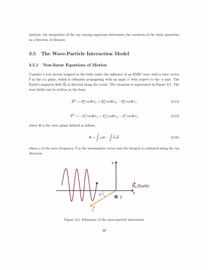
analysis, the integration of the ray tracing equations determines the variation of the these quantitiesas a function of distance.

3.5 The Wave-Particle Interaction Model

3.5.1 Non-linear Equations of Motion

Consider a test proton trapped in the belts under the influence of an EMIC wave with a wave vectork in the x-z plane, which is obliquely propagating with an angle ψ with respect to the -z axis. TheEarth’s magnetic field B0 is directed along the z-axis. The situation is represented in Figure 3.5. Thewave fields can be written in the form

Bw = Bwx cosΦ ex +Bw

y sinΦ ey −Bwz cosΦ ez (3.14)

Ew = −Ewx sinΦ ex + Ew

y cosΦ ey − Ewz sinΦ ez (3.15)

where Φ is the wave phase defined as follows

Φ =

ˆωdt−

ˆk· dr (3.16)

where ω is the wave frequency, k is the wavenumber vector and the integral is evaluated along the raydirection.

z!

x!

"!

B0 (Earth)!

k!

!!!y!

Figure 3.5: Schematic of the wave-particle interaction

39

The magnitude of the wave polarization ratios can be found from Maxwell’s equations and are givenby

Ewx

Ewy

=S − n2

D(3.17)

Ewz

Ewy

=

S − n2

n2sinθcosθ

D (n2sin2θ − P )(3.18)

Bwx

Bwy

= −D

n2sin2θ − P

P (S − n2)(3.19)

Bwz

Bwy

= −tanθD

n2sin2θ − P

P (S − n2)(3.20)

where n is the refractive index defined in Eq. 1.26 and P, S and D have been defined in Eqs. 1.23 to1.25.

The wave fields given above can be expressed as a sum of right and left circularly polarized components

Bw = BR + BL − ezBwz cosΦ (3.21)

where

BR =Bw

x +Bwy

2(excosΦ+ eysinΦ) (3.22)

BL =Bw

x −Bwy

2(excosΦ− eysinΦ) (3.23)

At a fixed point in space, BR rotates counterclockwise about B0 with angular velocity ω, while BL

rotates clockwise.

The Earth’s magnetic field is assumed to be locally parallel to the z-axis and vary slowly along it asfollows

B0 (r) = B0z (z) + B0⊥ (x, y, z) (3.24)

where B0⊥ for a dipole model can be evaluated using a Taylor expansion in x and y

40

B0⊥ (x, y, z) = − (excosξ + eysinξ) (x cosξ + y eysinξ)∂B0z

∂z(3.25)

where ξ is the angle between the magnetic meridional plane and the x-z plane.

We must mention here that all these equations including the dispersion relation in Section 1.2.4 arederived for an homogeneous medium. However, since the spatial variations of the plasma density andEarth’s magnetic field are small over the distance of the order of the wavelength, at any given point wecan assume that the wave has the same characteristics as those of a wave traveling in an homogeneousmedium with the same refractive index. This constitutes the slowly varying approximation, which iscommonly known as WKB approximation.

According to the resonance condition given in Eq. 1.36, protons must travel in the opposite directionto the waves, causing an upward Doppler shift on the frequency. Substituting these expressions intothe Lorentz force equation (Eq. 1.35) we get the following scalar equations of motion of the travelingparticle

px = −qEwx sinΦ+

q

mpγ

py (−Bw

z cosΦ+B0z)− pzBw

y sinΦ+B0⊥y

(3.26)

py = qEwy cosΦ+

q

mpγ[−px (−Bw

z cosΦ+B0z) + pz (Bwx cosΦ+B0⊥x)] (3.27)

pz = −qEwz sinΦ+

q

mpγ

px

Bw

y sinΦ+B0⊥y

− py (B

wx cosΦ+B0⊥x)

(3.28)

which can be expressed in terms of parallel and perpendicular momentum to the Earth’s magneticfield. Since the resonant interaction between a test proton and EMIC waves happens when the particlegyration is in phase with the left-hand elliptically polarized component of the wave, the angle inbetween BL and p⊥ (ϕ) is the most appropriate third component to use in the derivation of theequations of motion. This angle is represented in Figure 3.6.

41

BR!

x!

"!

y!

BL!

Bw!

v| - "!

!

#

Figure 3.6: Phase geometry of the interaction process

Taking into account that

px = p⊥cosθ (3.29)

py = p⊥sinθ (3.30)

θ = ϕ− Φ (3.31)

Φ = ω − v·k = ω + vxkx + vzkz (3.32)

the scalar equations of motion can be expressed as follows

ϕ = θ + Φ = −ωcp

γ+ ω + vxkx + vzkz +

C1

γ(3.33)

pz = −qEwz sinΦ− 1

γω1p⊥sin (ϕ− 2Φ)− 1

γω2p⊥sinϕ+ C2 (3.34)

p⊥ = ω1

pzγ

+R1mp

sin (ϕ− 2Φ) + ω2

pzγ

−R2mp

sinϕ+ C3 (3.35)

where mp and ωcp are the mass and cyclotron frequency of protons and

42

ω1 =q

mp

Bwx +Bw

y

2, ω2 =

q

mp

Bwx −Bw

y

2(3.36)

R1 =Ew

x + Ewy

Bwx +Bw

y

, R2 =Ew

x − Ewy

Bwx −Bw

y

(3.37)

C1 =q

mp

pzp⊥

[B0⊥xcos (ϕ− Φ) +B0⊥ysin (ϕ− Φ)] (3.38)

C2 =q

mpγp⊥ [B0⊥ycos (ϕ− Φ)−B0⊥xsin (ϕ− Φ)] (3.39)

C3 =q

mpγpz [B0⊥xsin (ϕ− Φ)−B0⊥ycos (ϕ− Φ)] (3.40)

In must be noted that in the equation for ϕ only the first order terms have been kept (we have neglectedthe effect of the wave-field on the equation for ϕ). These equations can be simplified by takingthe average over the particle gyroperiod. This approximation can be done if the gyroperiod of theproton is short compared to the time scale of the wave particle interaction. This approximation seemsvery reasonable and will be checked when solving the wave-particle interaction problem numerically.Following Jasna’s formulation [92], we introduce three new variables

χ =

ˆkxdx ⇒ χ = kxvx (3.41)

ϕ = η + χ ⇒ ϕ = η + χ (3.42)

ϕ = −ωcp

γ+ ω + vxkx + vzkz ⇒ ϕ = −ωcp

γt+ Φ+ Φ0 − ϕ0 (3.43)

Φ =ωcp

γt+ θ0 + ϕ = σ + ϕ = σ + η + χ (3.44)

σ =ωcp

γt+ θ0 , θ0 = ϕ0 − Φ0 (3.45)

and substituting into Eqs. 3.33 to 3.35, we can rewrite the equations of motion as follows

43

η = −ωcp

γ+ ω + vzkz +

C1

γ(3.46)

pz = ω2τ0

1

kz[−α1sin (η + χ)− γα2sin (σ + η + χ) + sin (2σ + η + χ)] + C2 (3.47)

p⊥ = −ω1

pzγ

+R1mp

sin (2σ + η + χ) + ω2

pzγ

−R2mp

sin (η + χ) + C3 (3.48)

where

ω2τ0 =

ω1kzp⊥γ

, α1 =ω2

ω1, α2 =

qEwz

ω1p⊥(3.49)

Using the fact that

χ =

ˆkxdx = kxv⊥

ˆcos (ϕ− Φ) dt = kxv⊥

ˆcos (σ) dt = β sinσ (3.50)

where β = γkxv⊥/ωc, and taking into account that

eiβsinσ =m=∞

m=−∞Jm (β) eimσ (3.51)

the gyroaveraged equations of motion can be written as follows

η = −ωcp

γ+ ω + vzkz +

C1

γ(3.52)

pz = ω2τ0

1

kz[−α1J0 (β) + γα2J1 (β) + J2 (β)] sinη + C2 (3.53)

p⊥ =

−ω1

pzγ

+R1mp

J2 (β) + ω2

pzγ

−R2mp

J0 (β)

sinη + C3 (3.54)

where Jν (β) are the Bessel functions of order ν and argument β and

C1 = 0 (3.55)

44

C2 = − 1

γmp

p2⊥2ωc

∂ωc

∂z(3.56)

C3 =1

γmp

p⊥pz2ωc

∂ωc

∂z(3.57)

From these equations we can see that the usefulness of η arises from the fact that η ≈ η and it can beinterpreted as the value of ϕ averaged over one gyroperiod.

3.5.2 Interaction with Individual Test Particles

When integrated over time, the equations of motion derived above determine the velocity space trajec-tories of individual test particles. This is the starting point of our study, which concerns the interactionbetween single particles and EMIC waves.

Previous studies of interaction between Whistlers and electrons [50] showed that the scattering isstrongly dependent on initial Larmor phase, thus we expect a similar behavior for EMIC-proton inter-action. For this reason, we will study protons at the edge of the loss cone, with different energies anddistributed uniformly over initial phase.

In order to find the total scattering, the field line is discretized in latitude and the equations of motionare integrated along that path. This procedure is repeated for each test particle. Using the adiabaticmotion relations, the integrated pitch angle and parallel velocity at each point along the path can bereferred to the equator and compared to the initial equatorial values in order to find the total scatteringand energy change of the particle.

The main result of this study is the region in velocity and pitch angle space that includes all particlesthat can resonantly interact with the radiated waves and that could be scattered into the loss cone.This information will be used as an input to the analysis of the full distribution of particles detailedin the next section.

3.5.3 Interaction with a Full Distribution of Particles

The test particles’ study illustrates the dynamics of the interaction and provides information aboutthe velocity and pitch angle space that includes all resonant particles. However, the analysis of the fulldistribution is required to assess the effects of EMIC waves on the population of energetic particles interms of precipitated fluxes and lifetimes.

The trapped population of energetic particles along a geomagnetic field line can be represented by adistribution function at the equator f (E,α) in part/

(m/s)3 m3

. However, experimental data are

45

often given in terms of the differential energy flux spectrum ΦE in part/m2s sr J

. We can relate

these two quantities using conservation of particles as follows

ΦE (E,α) dAdΩ dE dt = f (E,α) v2 dv dΩ vdt dA (3.58)

where dΩ is the element of solid angle and v is the magnitude of the velocity of a particle with energyE. Noting that dE = mγ3

Ev dv, where γE is the relativistic factor associated with E, we find thefollowing relation

f (E,α) = ΦE (E,α)mγ3

E

v2(3.59)

The differential precipitated flux Φ in part/m2s J

can be obtained by integrating the wave-perturbed

ΦE over the solid angle representing the loss cone, which is given by dΩ = sinα dα dφ. The parallelflux includes cosα to project along the B0 tube. In addition, the result needs to be multiplied byBTP /Beq, which accounts for the reduction of the flux tube cross section; using Eq. 3.1 it can beshown that BTP /Beq =

√1 + 3sin2λTP /cos6λTP , where λTP is the latitude at 100 km. The integral

can be expressed as follows

Φ (E) = 2π

√1 + 3sin2λTP

cos6λTP

ˆ αlc

0ΦE (E,α) cosα sinα dα (3.60)

and the number flux of precipitated particles N in part/m2s

would be

N =

ˆEΦ (E) dE (3.61)

and the associated energy flux Q in J/m2s

Q =

ˆEE Φ (E) dE (3.62)

We must note that by changing the limits of integration of N and Q we can explore the energydependence of these two quantities. In addition, for the case of a traveling pulse (instead of a steadystate case), all these quantities would be dependent on the time after pulse transmission.

The full distribution is simulated by a large number of individual test particles. For the high-energypopulation trapped in every flux tube, the distribution can be specified with its equatorial valuefeq (vII0eq,α0eq). From now on, we will drop the subscript eq. For a given field line and wave, onlya portion of the total population is scattered by the wave. Therefore, we only need to consider that

46

portion of the distribution. These bounds are the result of the analysis of individual test particletrajectories. After the non-perturbed distribution is specified, each test particle is allowed to gothrough a complete interaction by solving the non-linear equations of motion between two pointsalong a given field line. At the end of the interaction, each test particle would have acquired a newparallel velocity and pitch-angle, which can be identified with a mesh point (vIIF ,αF ) at the equator.This means that all the particles represented by this test particle have acquired parallel velocities andpitch angles between vIIF ±(∆vII/2) and αF ±(∆α/2) . Finally, in order to conserve the total numberdensity of particles in the system, the distribution function at (vII0,α0) and at (vIIF ,αF ) needs to bemodified as follows

fnew (vII0,α0) = fold (vII0,α0)−1

nφfold (vII0,α0) (3.63)

fnew (vIIF ,αF ) = fold (vIIF ,αF ) +1

nφfold (vII0,α0)

v2II0sinα0cos3α0

v2IIFsinαFcos3αF

(3.64)

where nφ is the number of particles per cell uniformly distributed in phase angle. The perturbeddistribution is obtained by using nφ test particles per mesh point and repeating the procedure forevery mesh point.

47

Chapter 4

Results to Date

Together with the formulation and conclusions presented in Chapters 1 and 3, my work to date con-sisted of the development of a wave-particle interaction code. My strategy starts by reproducingprevious work of whistlers interacting with electrons, which allows one to validate the approach andmethodology. Once the different aspects of this interaction have been checked with previous publica-tions I can safely start changing the wave dispersion, propagation and target particles to address ourproblem. So far I have reproduced most of the work relative to whistlers (without ray-tracing of thewaves) interacting with electrons using a formulation based on non-linear equations of motion, an Ihave started introducing the new EMIC regime and proton interaction. Some of the results obtainedso far are presented next.

4.1 Whistlers and Electrons

My first step was to reproduce the very first test particle formulation from Inan, 1978 [56]. In hiswork, Inan studied the non-linear, non-relativistic cyclotron resonant interaction between electronswith coherent and ducted Whistler waves in steady state. He developed a test particle simulationto solve the non-linear equations of motion and calculated the precipitated energy fluxes due to theinteraction with a full distribution of energetic particles. My first implementation reproduced theseresults, which are represented in Figures 4.1 and 4.2. The first plot gives the final net scattering atL = 4 (neq = 400 el/cm3) of a single resonant sheet of electrons uniformly distributed in Larmor phaseφ, with an initial equatorial pitch angle of αeq0 = 10 and moving away from the equator. The waveis characterized by Bweq = 20 pT and f = 5 kHz, and the velocity of the particles is such that theinteraction starts at the equator, which allows to clearly present the initial phase dependence. The

48

results are obtained by integrating the full equations of motions for each of the test electrons. In thispicture we can observe that the interaction is non-linear and the scattering is larger at φ0 ≈ 0 due toa trapping process that occurs at preferential phases where most of the cumulative interaction takesplace (phase trapping). Non-linear effects appear when the wave forces are the dominant factor incontrolling the phase rather than the inhomogeneity of the geomagnetic field, which begins to happenfor wave amplitudes greater than Bweq = 3 pT .

−200 −150 −100 −50 0 50 100 150 200−10

−8

−6

−4

−2

0

2

4

!0 [deg]

"#

eq [d

eg]

Scattering for Bw = 0.02 [nT] and #eq0 = 10 [deg]

Figure 4.1: Total scattering versus initial phase for equatorially resonant electrons with αeq0 = 10,wave intensity of Bw = 20 pT and f = 5 kHz

Figure 4.2 shows the equatorial distribution of particles integrated over parallel velocities between 1to 2 keV. The distribution before (blue) and after (red) the interaction with a Bweq = 30 pT wave ispresented. Particles are considered to be precipitated if their equatorial pitch angle after the interactionis smaller than the equatorial loss cone angle. Only the part of the distribution able to interact withthis wave has been considered, which is uniform in pitch angle and has a sharp cutoff at the losscone. We observe that as a result of the interaction, particles have been scattered into the loss cone.The energy flux of precipitated particles can be calculated according to Section 3.5.3, which givesQ = 0.2 J/

m2s

for Bweq = 30 pT , in accordance with Inan’s results.

49

1 2 3 4 5 6 7 8 9 10 11 120

0.2

0.4

0.6

0.8

1

1.2

! [deg]

f(!)

Normalized partile distribution f(!) for Bw = 3e−11 T

Non−perturbed distributionWave−perturbed distribution

Figure 4.2: Non-perturbed and perturbed particle distribution versus equatorial pitch angle for Bw =30 pT and f = 5 kHz

The next step in the implementation was to include the temporal variation of the precipitated fluxas a result of the interaction of short-duration Whistler pulses with energetic electrons [55] instead ofconsidering steady state. Figure 4.3 shows the precipitated energy flux versus time after transmissionof the wave injected at 1000 km of altitude at L = 4 for Bweq = 5 pT at the equator and f = 6.83 kHz.The responses were calculated for pulse-front locations between −16 and 44 of latitude. It can beobserved that the total length of the precipitated pulse is about 4 seconds, and the flux peaks at 3.5seconds. This maximum is the result of a convergence effect due to the responses’ overlap at differentpulse locations (thus different energies of interacting particles and different interaction lengths). Figure4.4 shows the energy of the particles that corresponds to that flux versus time after transmission (eachsegment represents a step in the pulse location).

50

0 0.5 1 1.5 2 2.5 3 3.5 4 4.5 50

0.005

0.01

0.015

0.02

0.025

Time [s]

r(t) [

ergs

/(cm

2 s)]

Transient precipitated energy flux at L = 4 for Bw = 5e−012 T (Inan82)

Figure 4.3: Precipitated energy flux versus time after the injection of the wave for Bw = 5 pT andf = 6.83 kHz

0 0.5 1 1.5 2 2.5 3 3.5 4 4.5 50

10

20

30

40

50

60

Time [s]

Ener

gy o

f pre

cipi

tatin

g pa

rticl

es [k

eV]

Energy of precipitating particles at L = 4 for Bw = 5e−012 T (Inan82)

Figure 4.4: Energy of the particles that constitue the flux of Figure 4.3

51

The next analysis incorporated relativistic effects to the previous formulation. This work was developedin the past by Chang, 1983 [24] for the steady state case. The same author addressed the transientcase in 1985 [26]. It must be noted here that relativistic effects are important when dealing with theenergetic population of electrons trapped in the belts. However, these corrections would not be requiredwhen targeting energetic protons because their energy can be larger than the ones of electrons buttheir velocities are non-relativistic. Figure 4.5 presents the energy spectrum of near-loss-cone quasi-relativistic electrons for the steady state case at L = 2 (neq = 800 el/cm3), for a wave intensity ofBweq = 7.5 pT and f = 5.46 kHz. The interaction takes into account two single passes, one at each sideof the equator, and the number of lobes and width depends of the distance between these resonances.

520 525 530 535 540 545 5500

20

40

60

80

100

120

140

160

180

E [keV]

q E [el c

m−2

s−1

keV

−1]

Energy spectrum of precipitating particles

Figure 4.5: Energy spectrum of precipitating particles

Figures 4.6 to 4.8 reproduce Chang’s results for relativistic electrons interacting with a 0.5 secondsWhistler pulse which enters the magnetosphere at 1000 km of altitude and propagates along L = 4

(neq = 400 el/cm3). The wave magnetic field intensity and frequency at the equator are taken to beBweq = 5 pT and f = 2.5 kHz. As the input pulse propagates toward the equator, it first interacts withhigher energy electrons because the resonant electron energy decreases when approaching the equator(as indicated by the resonance condition in Eq. 1.28). These electrons arrive first to the precipitationregion near the wave injection point, and equatorial scattered particles arrive later. As the pulsetravels past the equator, it interacts again with higher energy electrons and, although interacting withthe wave at later times, they can overtake these electrons scattered earlier by the wave close to theequator. This explanation matches the results presented in Figure 4.6, where the dynamic spectra ofthe precipitated energy flux is presented versus the particles’ energy and the time after transmission.

52

Figures 4.7 and 4.8 present the integration of this spectra over energy and time, respectively.

020

4060

80100 0

0.51

1.52

2.53

0

0.5

1

1.5

2

2.5

x 10−9

Time [s]

Dynamic spectra of the wave induced flux at L = 4 for Bw = 5e−012 T and E0 = 100 keV (Chang85 − Figure 5)

Energy [keV]

QE [e

rgs/

(cm

2 s k

eV)]

Figure 4.6: Dynamic spectra of the wave induced flux for Bw = 5 pT and E0 = 100 keV

0 0.5 1 1.5 2 2.5 3 3.5 4 4.5 50

1

2

3

4

5

6

7x 10−8

Time [s]

r(t) [

ergs

/(cm

2 s)]

Transient precipitated energy flux at L = 4 for Bw = 5 pT and E0 = 100 keV

Figure 4.7: Transient precipitated energy flux for Bw = 5 pT and E0 = 100 keV

53

0 10 20 30 40 50 60 70 80 90 1000

0.2

0.4

0.6

0.8

1

1.2x 10−9

Energy [keV]

Qsp

ectra

[erg

s/(c

m2 k

eV)]

Spectrum of precipitating electrons at L = 4 for Bw = 5 pT and E0 = 100 keV

Figure 4.8: Spectrum of precipitating electrons for Bw = 5 pT and E0 = 100 keV

The effect of obliquely propagating Whistlers on electrons was introduced next. Figures 4.9 to 4.11reproduce the work by Ristic [92, ?], which modeled the interaction between Whistlers propagatingat a wave-normal angle of ψ = 60, f = 15.792 kHz and constant power flux of S = 8.1 pW/m2

and electrons with energies around 100 eV at L = 3. Figure 4.9 presents the scattering (upper plot)and parallel velocity change (lower plot) of a single sheet of particles as a function of latitude due tothat wave. The sheet corresponds to test electrons with the same initial velocity and pitch angle, anduniformly distributed in Larmor phase (each line corresponds to a different phase). We can observe thatthe scattering is strongly dependent on initial phase, and for the given parameters the rms scatteringof the sheet has a value of ∆αeq|rms = 1.04. For the same wave parameters, Figure 4.10 presentsthe perturbed distribution function referred to the equator after the interaction with the wave; we canobserve that some particles have precipitated inside the loss cone, which is located at αlceq = 8.62.Finally, Figure 4.11 presents the differential precipitated flux Φ(E) for the same case. The numberflux of precipitated particles can be found by integrating Φ(E) over energies around 100 eV; taking∆E = 0.2 eV , we get N = 35·104 el/

cm2s

.

54

−1 −0.8 −0.6 −0.4 −0.2 0 0.2 0.4 0.6 0.8 1−2

−1.5

−1

−0.5

0

0.5

1

Latitude [deg]

! "

eq [d

eg]

S = 8.1 pW/m2, test electrons of E = 0.1 keV and #wave = 60 deg (Jasna93)

−1 −0.8 −0.6 −0.4 −0.2 0 0.2 0.4 0.6 0.8 15.84

5.845

5.85

5.855

5.86

5.865

5.87

Latitude [deg]

v res a

nd v

II [106 m

/s]

S = 8.1 pW/m2 and test electrons of E = 0.1 keV and #wave = 60 deg (Jasna93)

vresvII

Figure 4.9: Scattering and parallel velocity of a sheet of electrons interacting with Whistlers withψ = 60, f = 15.792 kHz and S = 8.1 pW/m2 at L = 3

45

67

89

1011

5.845.85

5.865.87

5.885.89

5.9

x 106

0

1

2

3

x 10−4

!eq [deg]

Perturbed distribution function at L = 3 for "wave = 60 deg (Jasna93)

vIIeq [s]

f(!,v

II)

Figure 4.10: Perturbed distribution function due to a ψ = 60, f = 15.792 kHz and S = 8.1 pW/m2

Whistler wave at L = 3

55

99 99.5 100 100.5 101 101.50

5

10

15

20

25

30

35

40

45

Eeq [eV]

!E [1

08 el/(

cm2 *

s * k

eV)]

Precipitated differential energy spectrum at L = 3 for "wave = 60 deg (Jasna93)

Figure 4.11: Differential precipitated flux of electrons due to a ψ = 60, f = 15.792 kHz and S =8.1 pW/m2 Whistler wave at L = 3

4.2 EMIC and Protons

The analyses above relative to whistler-electron interaction allowed me to validate the methodologybeing developed. Although the whistler-electron picture is still not complete, I have most of theingredients to start analyzing the case of EMIC-protons. Next, I present my first steps in this direction,which address the implementation of the dispersion relation presented in Section 1.2.4 and the analysisof the resonance condition of protons and the EMIC wave band. This is an ongoing study that willresult in the compatible range of frequencies, particles’ energies and shells of operation input to thewave-particle interaction analysis. Figure 4.12 presents a specific case for L = 2. The resonant energyrequired for cyclotron interaction with MeV protons is plotted as a function of resonant latitude andfrequency. We observe that the required energy of the target particles increases with latitude anddecreases with frequency, which means that compared to resonance at higher latitudes, interaction atthe equator (longer resonance times, higher scattering) for a fixed target’s energy would require lowerfrequencies.

56

Figure 4.12: Resonant energy of protons for EMIC interaction versus resonant latitude and frequency

Similar to Inan’s studies for the whistler-electron case [50], we have analyzed the interaction of parallelpropagating EMIC waves and a single sheet of protons uniformly distributed in Larmor phase. Figure4.13 represents the RMS scattering referred to the equator versus the wave power flux for equatorialinteraction between protons at the edge of the loss cone and parallel propagating EMIC waves atL = 1.5. This analysis is useful because it shows the importance of the wave field term compared tothe basic geomagnetic field in the variation of the phase η defined in Eq. 3.42. This wave term hasbeen neglected in our derivation of the equations of motion for interaction with oblique EMIC waves(Eq. 3.52), but it has been included in this study of parallel propagation following the formulationin [50]. According to these results and for the given parameters, the wave field is proportional to thescattering for power fluxes ≤ 10−4W/m2; in the literature this regime is called “linear mode”, wherethe wave term in the equation for η can be neglected. This linear mode is equivalent to assume thatthe wave effects are so small that the variation of η is very close to what it would have been withoutwave.

57

10−12 10−10 10−8 10−6 10−4 10−2 10010−4

10−3

10−2

10−1

100

101

102

Power flux [W / m2]

! "

RM

S eq [d

eg]

L = 1.5, protons of E = 14.395 MeV, #wave = 0 deg and "0eq = "lceq

Figure 4.13: RMS pitch-angle scattering versus power flux for parallel EMIC-proton resonant interac-tion at the equator (L = 1.5)

According to these results and neglecting the wave term in the phase equation, Figure 4.14 presentsthe pitch-angle scattering referred to the equator versus latitude of a single equatorially (L = 1.5)resonant sheet of protons interacting with an oblique EMIC wave with a wave-normal angle of ψ = 80

and power flux of 8.1−6W/m2. These protons have their velocity vector at the equator along theedge of the loss cone and are uniformly distributed in Larmor phase (each curve corresponds to adifferent phase). The RMS scattering for this case equals ∆αRMS |eq = 0.06, which is one order ofmagnitude smaller than the scattering obtained for field aligned waves (∆αRMS |eq = 0.5) as shownin Figure 4.13. Finally, Figure 4.15 presents the maximum scattering of each of these protons in thesheet versus their initial Larmor phase. In this Figure we can perfectly observe the sinusoidal behaviorof the scattering characteristic of this linear behavior. When neglecting the wave term from the phaseequation, the variation in time of the parallel and perpendicular momentum (Eqs. 3.53 and 3.54)depend sinusoidally on the phase, where η is now non dependent on the wave field.

58

−20 −15 −10 −5 0 5 10 15 20−0.2

−0.15

−0.1

−0.05

0

0.05

0.1

0.15

Latitude [deg]

! "

eq [d

eg]

L = 1.5, S = 8.1e−06 W/m2, E = 14.395 MeV, #wave = 80 deg and "0eq = "lceq

Figure 4.14: Total pitch-angle scattering versus latitude for a oblique EMIC wave interacting withequatorially resonant protons (L = 1.5)

0 50 100 150 200 250 300 350−0.1

−0.08

−0.06

−0.04

−0.02

0

0.02

0.04

0.06

0.08

0.1

!0 [deg]

" #

eqto

t [deg

]

L = 1.5, S = 8.1e−06 W/m2, E = 14.395 MeV, $wave = 80 deg and #0eq = #lceq

Figure 4.15: Maximum pitch-angle scattering versus initial Larmor phase for a oblique EMIC waveinteracting with equatorially resonant protons (L = 1.5)

59

Chapter 5

Future Work and Proposed Schedule

The future tasks described along this proposal and their planning are summarized in Figure 5.1:

Feb Mar Apr May Jun Jul Aug Sep Oct Nov Dec Jan Feb Mar Apr MayOblique propagation whistlersEMIC and electrons, comparison with existing resultsEMIC non-relativistic protonsStudy of multiple resonancesEMIC with heavy ionsMagnetic dipole solution and estimation of radiation impedanceStudy EMIC dispersion in a multi-ion plasmaRay-tracing of EMIC waves

INTEGRATION OF MODELS

Translation to the same programming language and integrationIdentification of test caseTest case resultsEngineering implicationsCount rates of particles' detectorComparison of performance with natural precipitationProposalThesis

PROPOSAL DEFENSE

SPRING 2013

WRITING

INTERACTION

SPRING 2012 SUMMER 2012TASK

RADIATION

RESUTLS AND SCALING

JanFALL 2012

PROPAGATION

Figure 5.1: Tasks’ planning

60

Bibliography

[1] B. Abel and R. M. Thorne. Electron scattering loss in earth’s inner magnetosphere 1. Dominantphysical processes. Journal of Geophysical Research, 103(A2):2385–2396, 1998.

[2] J. M. Albert. Cyclotron resonance in an inhomogeneous magnetic field. Physics of Fluids B:

Plasma Physics, 5:2744, 1993.

[3] J. M. Albert. Analysis of quasi-linear diffusion coefficients. Journal of Geophysical Research,104(A2):2429–2441, 1999.

[4] J. M. Albert. Gyroresonant interactions of radiation belt particles with a monochromatic elec-tromagnetic wave. Journal of Geophysical Research, 105(A9):21191–21209, 2000.

[5] J. M. Albert. Nonlinear interaction of outer zone electrons with VLF waves. Geophys. Res. Lett.,29(8), 04 2002.

[6] J. M. Albert. Evaluation of quasi-linear diffusion coefficients for EMIC waves in a multispeciesplasma. Journal of Geophysical Research, 108, 06 2003.

[7] J. M. Albert. Evaluation of quasi-linear diffusion coefficients for whistler mode waves in a plasmawith arbitrary density ratio. Technical report, DTIC Document, 2005.

[8] J. M. Albert and J. Bortnik. Nonlinear interaction of radiation belt electrons with electromagneticion cyclotron waves. Geophysical Research Letter, 36, 06 2009.

[9] B. J. Anderson. Recent observations of electromagnetic ion cyclotron waves in space. Advances

in Space Research, 17(10):41–50, 1996.

[10] B. J. Anderson, R. E. Erlandson, and L. J. Zanetti. A statistical study of Pc 1-2 magneticpulsations in the equatorial magnetosphere, 2. Wave properties. Journal of Geophysical Research,97(A3):3089–3101, 1992.

62

[11] J. J. Angerami and J. O. Thomas. Studies of Planetary Atmospheres 1. The Distribution ofElectrons and Ions in the Earth’s Exosphere. Journal of Geophysical Research, 69(21):4537–4560, 1964.

[12] M. Ashour-Abdalla. Amplification of whistler waves in the magnetosphere. Planetary and Space

Science, 20(5):639 – 662, 1972.

[13] D. N. Baker. The occurrence of operational anomalies in spacecraft and their relationship tospace weather. Plasma Science, IEEE Transactions on, 28(6):2007–2016, 2000.

[14] D. N. Baker, R. D. Belian, P. R. Higbie, R. W. Klebesadel, and J. B. Blake. Deep dielectric charg-ing effects due to high-energy electrons in Earth’s outer magnetosphere. Journal of electrostatics,20(1):3–19, 1987.

[15] K. Balmain. The impedance of a short dipole antenna in a magnetoplasma. IEEE Transactions

on Antennas and Propagation, 12(5):605–617, September 1964.

[16] T. F. Bell. The nonlinear gyroresonance interaction between energetic electrons and coherentVLF waves propagating at an arbitrary angle with respect to the Earth’s magnetic field. Journal

of Geophysical Research, 89:905–918, 1984.

[17] T. F. Bell, U. S. Inan, and T. Chevalier. Current distribution of a VLF electric dipole antennain the plasmasphere. Radio Science, 41(2), 04 2006.

[18] T. F. Bell, U.S. Inan, J. Bortnik, and J. D. Scudder. The landau damping of magnetosphericallyreflected whistlers within the plasmasphere. Geophysical research letters, 29(15):23–1, 2002.

[19] T. F. Bell and T. Wang. Radiation resistance of a small filamentary loop antenna in a coldmulticomponent magnetoplasma. IEEE Transactions on Antennas and Propagation, 19(4):517–522, 1971.

[20] J. Bortnik, U. S. Inan, and T. F. Bell. Temporal signatures of radiation belt electron precipitationinduced by lightning-generated MR whistler waves: 1. Methodology. Journal of Geophysical

Research, 111, 2006.

[21] W. L. Brown and J. D. Gabbe. The electron distribution in the Earth’s radiation belts duringJuly 1962 as measured Telstar. Journal of Geophysical Research, 68(3):607–618, 1963.

[22] K.G. Budden. Radio waves in the ionosphere. Cambridge University Press, 1966.

[23] H. C. Chang. Cyclotron Resonant Scattering of Energetic Electrons by Electromagnetic Waves

in the Magnetosphere. PhD thesis, Stanford University, 09/1983 1983.

63

[24] H. C. Chang and U. S. Inan. Quasi-relativistic electron precipitation due to interactions withcoherent VLF waves in the magnetosphere. Journal of Geophysical Research, 88:318–328, 1983.

[25] H. C. Chang and U. S. Inan. Lightning-induced electron precipitation from the magnetosphere.Journal of Geophysical Research, 90:1531–1541, 1985.

[26] H. C. Chang and U. S.. Inan. Test particle modeling of wave-induced energetic electron precipi-tation. Journal of Geophysical Research, 90:6409–6418, 1985.

[27] T. W. Chevalier, U. S. Inan, and T. F. Bell. Fluid simulation of the collisionless plasma sheathsurrounding an electric dipole antenna in the inner magnetosphere. Radio Science, 45:1010, feb2010.

[28] T. W. Chevalier, U. S. Inan, and T. F.F. Bell. Terminal impedance and antenna current distri-bution of a VLF electric dipole in the inner magnetosphere. Antennas and Propagation, IEEE

Transactions on, 56(8):2454 –2468, 2008.

[29] D. Cohen, G. Spanjers, J. Winter, G. Ginet, B. Dichter, A. Adler, and M. Tolliver. Design andSystems Engineering of AFRL’s Demonstration and Sciences Experiment. 2005.

[30] A. C. Das. A mechanism for VLF emissions. Journal of Geophysical Research, 73(23):7457–7471,1968.

[31] M. De Soria-Santacruz. Radiation of VLF/ELF waves from a magnetospheric tether. Master’sthesis, Massachusetts Institute of Technology, June 2011.

[32] K. Dobes. The HM wave-particle cyclotron resonance for non-parallel propagation. Planetary

and Space Science, 18(3):395 – 406, 1970.

[33] R. E. Erlandson and A. J. Ukhorskiy. Observations of electromagnetic ion cyclotron wavesduring geomagnetic storms: Wave occurrence and pitch angle scattering. Journal of Geophysical

Research, 106(A3):3883–3895, 2001.

[34] B. J. Fraser. Observations of ion cyclotron waves near synchronous orbit and on the ground.Space Science Reviews, 42(3):357–374, 1985.

[35] B. J. Fraser, J. C. Samson, Y. D. Hu, R. L. McPherron, and C. T. Russell. Electromagneticion cyclotron waves observed near the oxygen cyclotron frequency by ISEE 1 and 2. Journal of

Geophysical Research, 97(A3):3063–3074, 1992.

[36] B. J. Fraser, H. J. Singer, W. J. Hughes, J. R. Wygant, R. R. Anderson, and Y. D. Hu. CR-RES Poynting vector observations of electromagnetic ion cyclotron waves near the plasmapause.Journal of Geophysical Research, 101(A7):15331–15, 1996.

64

[37] G. P. Ginet and J. M. Albert. Test particle motion in the cyclotron resonance regime. Physics

of Fluids B: Plasma Physics, 3:2994, 1991.

[38] G. P. Ginet and M. A. Heinemann. Test particle acceleration by small amplitude electromagneticwaves in a uniform magnetic field. Physics of Fluids B: Plasma Physics, 2:700, 1990.

[39] G. P. Ginet, J. Stuart, A. Adler, D. Smith, M. Scherbarth, et al. AFRL’s Demonstration andScience Experiments (DSX) Mission. In Proceedings of SPIE, 2009.

[40] S. A. Glauert and R. B. Horne. Calculation of pitch angle and energy diffusion coefficients withthe PADIE code. Journal of Geophysical Research, 110(A4), 04 2005.

[41] L. Gomberoff and R. Neira. Convective Growth Rate of Ion Cyclotron Waves in a H+-He+ andH+-He+-O+ Plasma. Journal of Geophysical Research, 88(A3):2170–2174, 1983.

[42] J. Haselgrove. Ray theory and a new method for ray tracing. In Physics of the Ionosphere,volume 1, page 355, 1955.

[43] R. J. Hastie, J. B. Taylor, and F. A. Haas. Adiabatic invariants and the equilibrium of magnet-ically trapped particles. Annals of Physics, 41(2):302–338, 1967.

[44] R. B. Horne and R. M. Thorne. On the preferred source location for the convective amplificationof ion cyclotron waves. Journal of Geophysical Researchesearch, 98(A6):9233–9247, 1993.

[45] R. B. Horne and R. M. Thorne. Relativistic electron acceleration and precipitation duringresonant interactions with whistler-mode chorus. Geophysical Research Letters, 30(10):1527,2003.

[46] J. L. Horwitz, R. H. Comfort, P.G. Richards, M.O. Chandler, C.R. Chappell, P. Anderson, W. BHanson, and L. H. Brace. Plasmasphere-ionosphere coupling, 2. Ion composition measurementsat plasmaspheric and ionospheric altitudes and comparison with modeling results. Journal of

Geophysical Research, 95(A6):7949–7959, 1990.

[47] Y. D. Hu and B. J. Fraser. Group travel time of EM waves with frequencies near the ion cyclotronfrequency in the two-ion magnetosphere. Australian journal of physics, 45(5):695–716, 1992.

[48] N. D. Hulkower and R. J. Rusch. Study of Plasma Motor Generator (PMG) tether system fororbit reboost. 1987.

[49] W. L. Imhof, J. B. Reagan, H. D. Voss, E. E. Gaines, D. W. Datlowe, J. Mobilia, R. A. Helliwell,U. S. Inan, J. Katsufrakis, and R.G. Joiner. Direct observation of radiation belt electrons precip-itated by the controlled injection of VLF signals from a ground-based transmitter. Geophysical

Research Letters, 10:361–364, 1983.

65

[50] U. S. Inan. Non-linear gyroresonant interactions of energetic particles and coherent VLF waves

in the magnetosphere. Ph. d thesis, Stanford University, 1977.

[51] U. S. Inan. Gyroresonant pitch angle scattering by coherent and incoherent whistler mode wavesin the magnetosphere. Journal of Geophysical Research, 92:127–142, 1987.

[52] U. S. Inan and T. F. Bell. The plasmapause as a vlf wave guide. Journal of Geophysical Research,82(19):2819, 1977.

[53] U. S. Inan and T. F. Bell. Pitch angle scattering of energetic particles by oblique whistler waves.Geophysical Research Letters, 18:49–52, 1991.

[54] U. S. Inan, T. F. Bell, and J. Bortnik. Controlled precipitation of radiation belt electrons.Journal of Geophysical Research, 108(A5), 2003.

[55] U. S. Inan, T. F. Bell, and H. C. Chang. Particle precipitation induced by short-duration VLFwaves in the magnetosphere. Journal of Geophysical Research, 87:6243–6264, 1982.

[56] U. S. Inan, T. F. Bell, and R. A. Helliwell. Nonlinear pitch angle scattering of energetic electronsby coherent VLF waves in the magnetosphere. Journal of Geophysical Research, 83(A7):3235–3253, 1978.

[57] U. S. Inan, H. C. Chang, and R. A. Helliwell. Electron precipitation zones around major ground-based VLF signal sources. Journal of Geophysical Research, 89(A5):2891–2906, May 1984.

[58] U. S. Inan, F. Knifsend, and J. Oh. Subionospheric VLF ’imaging’ of lightning-induced electronprecipitation from the magnetosphere. Journal of Geophysical Research, 95:17217–17231, 1990.

[59] U. S. Inan and S. Tkalcevic. Nonlinear equations of motion for Landau resonance interactionswith a whistler mode wave. Journal of Geophysical Research, 87:2363–2367, 1982.

[60] V. K. Jordanova, C. J. Farrugia, J. M. Quinn, R. M. Thorne, K. E Ogilvie, R. P. Lepping, G. Lu,A. J. Lazarus, M. F. Thomsen, and R. D. Belian. Effect of wave-particle interactions on ringcurrent evolution for January 10-11, 1997: Initial results. Geophysical Research Letter, 25.

[61] V. K. Jordanova, C. J. Farrugia, R. M. Thorne, G. V. Khazanov, G. D. Reeves, and M. F.Thomsen. Modeling ring current proton precipitation by electromagnetic ion cyclotron wavesduring the May 14–16, 1997, storm. Journal of Geophysical Research, 106.

[62] V. K. Jordanova, J. U. Kozyra, and A. F. Nagy. Effects of heavy ions on the quasi-linear diffusioncoefficients from resonant interactions with electromagnetic ion cyclotron waves. Journal of

Geophysical Research, 101(A9):19771–19778, September 1996.

66

[63] V. K. Jordanova, J. U. Kozyra, A. F. Nagy, and G. V. Khazanov. Kinetic model of the ringcurrent-atmosphere interactions. Journal of Geophysical Research, 102.

[64] Adolph S. Jursa, editor. Handbook of geophysics and the space environment. Air Force ResearchLaboratory, US Air Force, Fourth edition, 1985.

[65] C. Kennel and H. Petschek. Limit on stably trapped particle fluxes. Journal of Geophysical

Research, 71(1):1–28, 1966.

[66] C. F. Kennel and F. Engelmann. Velocity space diffusion from weak plasma turbulence in amagnetic field. Physics of Fluids, 9(12):2377, 1966.

[67] G. V. Khazanov and K. V. Gamayunov. Effect of EMIC wave normal angle distribution onrelativistic electron scattering in outer RB. Technical report, NASA.

[68] G. V. Khazanov, K. V. Gamayunov, D. L. Gallagher, and J. U. Kozyra. Self-consistent modelof magnetospheric ring current and propagating electromagnetic ion cyclotron waves: Waves inmulti-ion magnetosphere. Journal of Geophysical Research, 111(A10), 10 2006.

[69] G. V. Khazanov, K. V. Gamayunov, V. K. Jordanova, and E. N. Krivorutsky. A self-consistentmodel of the interacting ring current ions and electromagnetic ion cyclotron waves, initial results:Waves and precipitating fluxes. Journal of Geophysical Research, 107(A6), 06 2002.

[70] GV Khazanov, KV Gamayunov, DL Gallagher, JU Kozyra, and MW Liemohn. Self-consistentmodel of magnetospheric ring current and propagating electromagnetic ion cyclotron waves:2. wave-induced ring current precipitation and thermal electron heating. J. Geophys. Res,112:A04209, 2007.

[71] H. C. Koons, B. C. Edgar, and A. L. Vampola. Precipitation of inner zone electrons by whistlermode waves from the VLF transmitters UMS and NWC. Journal of Geophysical Research,86(A2):640–648, 1981.

[72] H. H. Kuehl. Electromagnetic radiation from an electric dipole in a cold anisotropic plasma.Physics of Fluids, 5(9):1095–1104, 1962.

[73] P. Kulkarni, U. S. Inan, and T. F. Bell. Energetic electron precipitation induced by space basedVLF transmitters. Journal of Geophysical Research, 113, 2008.

[74] W. Li, Y. Y. Shprits, and R. M. Thorne. Dynamic evolution of energetic outer zone electronsdue to wave-particle interactions during storms. J. Geophys. Res., 112(A10), 10 2007.

[75] K. R. Lorentzen, M. P. McCarthy, G. K. Parks, J. E. Foat, R. P. Lin, R. M. Millan, D. M. Smith,and J. P. Treilhou. Precipitation of relativistic electrons by interaction with electromagnetic ioncyclotron waves. Journal of Geophysical Research-Space Physics, 105(A3):5381–5389, 2000.

67

[76] T. M. Loto’aniu, B. J. Fraser, and C. L. Waters. Propagation of electromagnetic ion cyclotronwave energy in the magnetosphere. Journal of Geophysical Research, 110, 07 2005.

[77] G. R. Ludlow. Growth of obliquely propagating ion cyclotron waves in the magnetosphere.Journal of Geophysical Research, 94(A11):15385–15391, November 1989.

[78] L. R. Lyons. General relations for resonant particle diffusion in pitch angle and energy. Journal

of Plasma Physics, 12(01):45–49, 1974.

[79] L. R. Lyons. Pitch angle and energy diffusion coefficients from resonant interactions with ion–cyclotron and whistler waves. Journal of Plasma Physics, 12(03):417–432, 1974.

[80] L. R. Lyons and R. M. Thorne. Parasitic pitch angle diffusion of radiation belt particles by ioncyclotron waves. Journal of Geophysical Research, 77(28), October 1972.

[81] L. R. Lyons, R. M. Thorne, and C. F. Kennel. Pitch-angle diffusion of radiation belt electronswithin the plasmasphere. Journal of Geophysical Research, 77(19):3455–3474, 1972.

[82] L. R. Lyons and D. J. Williams. The quiet time structure of energetic (35-560 keV) radiationbelt electrons. Journal of Geophysical Research, 80(7):943–950, 1975.

[83] N. P. Meredith, R. M. Thorne, R. B. Horne, D. Summers, B. J. Fraser, and R. R. Anderson.Statistical analysis of relativistic electron energies for cyclotron resonance with EMIC wavesobserved on CRRES. Journal of Geophysical Research, 108, 06 2003.

[84] Y. Miyoshi, K. Sakaguchi, K. Shiokawa, D. Evans, J. Albert, M. Connors, and V. Jordanova.Precipitation of radiation belt electrons by EMIC waves, observed from ground and space. Geo-

physical Research Letter, 35, 12 2008.

[85] F. S. Mozer, D. D. Elliott, J. D. Mihalov, G. A. Paulikas, A. L. Vampola, and S. C. Freden.Preliminary analysis of the fluxes and spectrums of trapped particles after the nuclear test ofJuly 9, 1962. Journal of Geophysical Research, 68(3):641–649, 1963.

[86] NASA. AE-8/AP-8 Radiation Belt Models.

[87] NASA Data Center National Space Science. Intercosoms 24, March 2012.

[88] T. G. Northrop. Adiabatic charged-particle motion. Reviews of Geophysics, 1(3):283–304, 1963.

[89] T. G. Northrop and E. Teller. Stability of the adiabatic motion of charged particles in the earth’sfield. Physical Review, 117(1):215, 1960.

[90] G. F. Pieper. A second radiation belt from the July 9, 1962, nuclear detonation. Journal of

Geophysical Research, 68(3):651–655, 1963.

68

[91] J. L. Rauch and A. Roux. Ray tracing of ULF waves in a multicomponent magnetospheric plasma:Consequences for the generation mechanism of ion cyclotron waves. Journal of Geophysical

Research, 87(A10):8191–8198, 1982.

[92] J. L. Ristic-Djurovic. Gyroresonant scattering of radiation belt electrons by oblique whistler waves.Ph. d thesis, Stanford University, May 1993.

[93] J. L. Ristic-Djurovic, U. S. Inan, and T. F. Bell. Precipitation of suprathermal(100 ev) electronsby oblique whistler waves. Geophysical research letters, 19(16):1639–1642, 1992.

[94] C. J. Rodger, M. A. Clilverd, Th. Ulich, P. T. Verronen, E. Turunen, and N. R. Thomson. Theatmospheric implications of radiation belt remediation. Ann. Geophys., 24:2025–2041, 2006.

[95] C. J. Rodger, T. Raita, M. A. Clilverd, A. Seppälä, S. Dietrich, N. R. Thomson, and T. Ulich.Observations of relativistic electron precipitation from the radiation belts driven by EMIC waves.Geophysical Research Letter, 35, 08 2008.

[96] J. Schoenberg. The Demonstration and Science Experiments (DSX): A Fundamental ScienceResearch Mission Advancing Technologies that Enable MEO Spaceflight. Technical report, DTICDocument, 2006.

[97] R. S. Selesnick, M. D. Looper, and R. A. Mewaldt. A theoretical model of the inner protonradiation belt. Space Weather, 5(4), 04 2007.

[98] D. R. Shklyar. Particle interaction with an electrostatic VLF wave in the magnetosphere withan application to proton precipitation. Planetary and Space Science, 34(11):1091 – 1099, 1986.

[99] DR Shklyar. Mechanism for proton precipitation triggered by a VLF wave injected into themagnetosphere. JETP Letters, 41:448–451, 1985.

[100] P. Song, B. W. Reinisch, V. Paznukhov, G. Sales, D. Cooke, J. N. Tu, X. Huang, K. Bibl, andI. Galkin. High-voltage antenna-plasma interaction in whistler wave transmission: Plasma sheatheffects. Journal of Geophysical Research, 112(A3), March 2007.

[101] G. Spanjers, J. Winter, D. Cohen, A. Adler, J. Guarnieri, M. Tolliver, G. Ginet, B. Dichter, andJ. Summers. The AFRL demonstration and science experiments (DSX) for DoD space capabilityin the MEO. In Aerospace Conference, 2006 IEEE, pages 10–pp. IEEE, 2006.

[102] R. L. Stenzel. Self-ducting of large-amplitude whistler waves. Phys. Rev. Lett., 35(9):574–577,Sep 1975.

[103] R. L. Stenzel. Antenna radiation patterns in the whistler wave regime measured in a largelaboratory plasma. Radio Science, 11(12):1045–1056, 1976.

69

[104] T. H. Stix. Waves in Plasmas. Springer-Verlag New York, Inc., 1992.

[105] D. Summers. Quasi-linear diffusion coefficients for field-aligned electromagnetic waves with ap-plications to the magnetosphere. J. Geophys. Res., 110, 08 2005.

[106] D. Summers and R. M. Thorne. Relativistic electron pitch-angle scattering by electromagneticion cyclotron waves during geomagnetic storms. Journal of Geophysical Research, 108(A4):1143,April 2003.

[107] Y. Takiguchi. Emission of whistler waves from an ionospheric tether. Master’s thesis, Mas-sachusetts Institute of Technology, September 2009.

[108] X. Tao and J. Bortnik. Nonlinear interactions between relativistic radiation belt electrons andoblique whistler mode waves. Nonlinear Processes in Geophysics, 17:599–604, 2010.

[109] R. M. Thorne and R. B. Horne. Cyclotron absorption of ion-cyclotron waves at the bi-ionfrequency. Geophysical Research Lettersesearch letters, 20(4):317–320, 1993.

[110] R. M. Thorne, R. B. Horne, V. K. Jordanova, J. Bortnik, and Glauert Sarah. Interaction ofEMIC Waves with Thermal Plasma and Radiation Belt Particles. Technical report, 2006.

[111] R. M. Thorne and C. F. Kennel. Quasi-trapped vlf propagation in the outer magnetosphere.Journal of Geophysical Research, 72(3):857–870, 1967.

[112] J. Tu, P. Song, and B. W. Reinisch. Plasma sheath structures around a radio frequency antenna.Journal of Geophysical Research, 113(A7), 07 2008.

[113] J. A. Van Allen, G. H. Ludwig, E. C. Ray, and C. E. McIlwain. Observation of high intensityradiation by satellites 1958 alpha and gamma. Jet Propulsion, 28(9):588–592, 1958.

[114] D. L. Voss, A. Gunda, D. Carssow, T. Fritz, A. Mavretic, and J. Sullivan. Overview of the losscone imager fixed sensor head instrument. In Proceedings of SPIE, volume 7438, page 743808,2009.

[115] M. Walt. Introduction to geomagnetically trapped radiation, volume 1. 2005.

[116] T. Wang and T. Bell. VLF/ELF input impedance of an arbitrarily oriented loop antenna in a coldcollisionless multicomponent magnetoplasma. IEEE Transactions on Antennas and Propagation,20(3):394 – 398, may 1972.

[117] T. Wang and T. Bell. On input impedance of an arbitrarily oriented small loop antenna in a coldcollisionless magnetoplasma. IEEE Transactions on Antennas and Propagation, 21(5):745–746,1973.

70

[118] T. N. C. Wang and T. F. Bell. Radiation resistance of a short dipole immersed in a coldmagnetoionic medium. Radio Science, 4(2):167–177, 1969.

[119] T. N. C. Wang and T. F. Bell. On VLF radiation resistance of an electric dipole in a coldmagnetoplasma. Radio Science, 5(3):605–610, 1970.

[120] T. N. C. Wang and T. F. Bell. Electric dipole radiation at VLF in a uniform warm magneto-plasma. Revue de Physique Appliquee, 7(1):11–20, 1972.

[121] T. N. C. Wang and T. F. Bell. VLF/ELF Radiation Patterns of Arbitrarily Oriented Electric andMagnetic Dipoles in a Cold Lossless Multicomponent Magnetoplasma. Journal of Geophysical

Research, 77(7):1174–1189, March 1972.

[122] A. G. Yahnin and T. A. Yahnina. Energetic proton precipitation related to ion-cyclotron waves.Journal of Atmospheric and Solar-Terrestrial Physics, 69(14):1690–1706, 10 2007.

[123] D. T. Young, S. Perraut, A. Roux, C. de Villedary, R. Gendrin, A. Korth, G. Kremser, andD. Jones. Wave-Particle Interactions near &#937;He+ Observed on GEOS 1 and 2, 1. Propaga-tion of Ion Cyclotron Waves in He+-Rich Plasma. Journal of Geophysical Research, 86(A8):6755–6772, 1981.

71