NUC TP 504

ELECTROMAGNETIC FIELDS IN THE OCEANAND ELECTRO RECEPTIVE FISH

00 byE. H. Satorius

0 Undersea Sciences Department

February 1976

le

R DDCVJ7ILf

n~U21

ZvAppove Do pulCrlae itrbto niieI,

~1n

U: AG2517

- .N

NAVAl UNOERSIA CENTER. SAN DIEGO CA. 92132

AN ACTIVITY OF THE NAVAL MATERIAL COMMAND

R. B. GILCHRIST, CAPT, USN HOWARD L. BL000, PhDCommander Technkal Director

ADMINISTRATIVE STATEMENT

The work reported herein was conducted during Fiscal Year 1976 at the NUCMarine Life Sciences Laboratory as part of two projects: Electrosensory reception, ProjectNo. SF34371403, sponsored by the Naval Sea Systems Command, and an IndependentResearch project on Electroreception, S. H. Ridgway, Principal Investigator.

Released by Under Authority ofC. S. Johnson B. A. PowellAssociate for Applied Sciences Head, Undersea Sciences Department

ACKNOWLEDGMENTS

The author wishes to thank R. Seeley, W. Flanigan, S. Ridgway, C. S., Johnson,D. Carder, W. Lowell, W. Kordela, B. Gordon, G. Lindsay, and E. Knudson, for many helpfuldiscussions concerning this report.

- ---

..... ... ..........

911I1111TI1,rAV AILA3ILIlt cg[I.

ii

UNCLASSIFIEDSECURITY CLASSIFICATION OF THIS PAGE (When. niet. FKniid)

2 GOVT A:CCSSION NO .4_MCIVIENT'S CATALOG NUMBER

-ELCTROMAGNETKI JELDS IN TECAN ANDI Jul75 iu764FEECTRRECEPT1V~ISZH, ---- "

TACT RR CAIN

K.M U"I USR

It CONTROLLING OPPIC9 NAME AND AODES 0

Naval Sea Systems Command F eb 0 I* !Wa4.ington, D.C. / low

14 MONITORING AGENCY NAME 4 AODRES-YOI d.tiff,.I If- C.A01,.I10"S Office) It SECURITY CL ASS (.1 Ohio ropon

&1 36. 44 DEIC IASSI iCATtON DOW14GRAD NG

17 DISTRIBUTION STATEMENTY (.1Ikeb.~y O.O Z , Iy O. .1 dillo...,' ho- Riowlt)

10 SUPPLEMENTARY NOTES

IS KEY WORDS (C-fi.n. . .* I n rid *dl-t by block .-unbe,)

ocean electromagnetic noise fields N

electrosensing skates and sl'arks /a'r~ k~,~f'~

20 ABSTRACT (Cornisnu.o,, r,.... side Ifi rcitsoty asid ,denltt by block swunbor)

This report considers the possibility of the detection of dipole fields by elect rosensming- fish. In particular, a skate (Raja clavata) which is sensitive to threshold electric fields of puv in

has been examined. The results indicate that skates detect electric dipole fields at short is-tances (approximately 100 mn at f0O, 1, or 10 H~z and for dipole source current moments on theorder of 60 A-rn). A comparison between the electnic dipole sensing capabilities of skates andartificial systems is also made. In general, it appears that the optimum single-element man-made sensing system is supe~ior to the skate for purposes of long-range detection of

D JN 1473 P, EDITION 01 -0NV 11S IS OBSOLETE UNCLASSIFIEDSECURNITY CLASSIFICATION OF THIS PAGE I~hbrn Date Fnitered)

LNCLASSIFIEDsecuphlY CLA*SSWICATI@W of, Tools 9A(WWW. 09. &100",)

20(cont)narrowband, extremely low-frequency signals.

UNCLASSIFIEDSECURITY CLASSIrICATION OF THIS PACVEWhen 0ots FI1eSed)

TABLE OF CONTENTSPage

1.: INTRODUCTION I

2. A REVIEW OF PASSIVE ELECTRORECEPTION BY ELECTRORECEP-TIVE FISH 3

3., ELECTROMAGNETIC DIPOLE FIELDS IN THE OCEAN (NOBOUNDARY EFFECTS) AND THEIR DETECTION BY SKATES 5

A. A Brief Summary of Electromagnetic Wave Propagation in the Ocean 5B. Electric Dipole Fields in the Ocean 7C. Magnetic Dipole Fieldb in the Ocean 12

4. ELECTROMAGNETIC WAVES TRAVELING ALONG THE OCEAN'SSURFACE AND THE POSSIBILITY OF THEIR DETECTION BY SKATES 17

5. A COMPARISON BETWEEN THE ELECTRIC-SENSING CAPABILITIESOF SKATES AND ARTIFICIAL SYSTEMS 23

6. CONCLUSIONS 31

Summary 31Suggestions for Further Work 31

REFERENCES 33

ii

1. INTRODUCTION

In this report a study is made of extremely low-frequency (f 10 Hz) electromag-netic fields in the ocean produced by dipole currents and the possibility of these fieldsbeing sensed by electroreceptive fish at various distances from the dipole sources. In Sec-tion 2, a brief review of the mechanism for extremely low-frequency passive electrorecep-tion by electroreceptive fish is presented. In particular, the electroreception capabilities of ashark, Scyliorhinus canicula, and skate, Raja clavata, are evaluated. These fish are usuallyfound at the ocean bottom near shore lines and in bays. From an electrical field point ofview they are very interesting in that they can sense electric fields as weak as I AV/m.* Sec-tion 3 of this report deals quantitatively with the electromagnetic fields generated by dipolesources deep in the ocean (i.e., far enough away from ocean-air or earth-ocean boundaries sothat boundary effects can be ignored), and the possible detection of these fields by skates. InSection 4, surface electromagnetic waves propagating along the ocean-air interface generat-ed by dipole sources are examined and the possible detection of these surface waves byskates is considered. Finally, in Section 5, a comparison is made of the extremely low-frequency electric-dipole sensing capabilities of skates with the capabilities of man-madeextremely low-frequency, electric dipole sensing systems. Sensitivity .nd environmentalnoise will be the primary considerations in making this comparison.

*The threshold of the skate Raja clavata has been measured as low as I A Vim The threshold of the shark Scyliorhinus

caficula has been measured at 10 V/rm The threshold value of I MV/m for the skate represents the highest electricalsensitivity known in aquatic animals (Ref 1)

2. A REVIEW OF PASSIVE ELECTRORECEVI ION BY ELECTRORECEPTIVE FISH

Certain types of fish have a passive electrosensing mechanism by which they cansense electric fields of very low magnitude. In general, this sensing mechanism is responsiveto extremely low-frequency electric fields (f 10 Hz) at amplitudes (thresholds) whichrange from 12.5 V/rn for Rhodeus sericeus down to 1 uV/m for Raja clavata (Ref. 1). The'I electric receptors which make up this electrosensing mechanism in sharks and skates tLavebeen identified by Kalmijn (Ref. 4) as the ampullae of Lorenzini.* These ampullae are tinybladders which are innervated by sensory cells and are connected to surface pores by longcanals with highly resistive walls. Each canal is filled with a highly conductive jelly. Onesitle of each of the sensory cells at the bottom of an ampulla is in contact with this jelly,while the other side is in contact with body fluid. When a voltage gradient is applied alongthe length of one of these electroreceptors, the jelly-side of these sensory cells is at thepotential of the jelly nearest the bottom of the amnulla. However, being a good conductor,the jelly nearest the bottom of the ampulla is at the same potential as the seawater at thesurface-pore end of the canal (see Fig. 1),. The body-fluid side of the sensory cels is at

*A ctually, certainfrub have passive electrosen sing -Ysi'ems which are sensitive to electric fields of much higher frequenciest6&0~200 Hz). The electroreceptors which make up this electrosensing system are tuberous sense organs (Ref. 2) This

f report wil! concern only the passive electrosensing of extremely low-frequency fields (f~ 10 Hz) by ampullary senseOrgans.

Lnits of voitage

+6 __ +4_ +3-+2 _.~..+i____ -I ... 2.....3_ -4 __ -5_.....6

I I I I seawater

anode cathode

Figure I Cross section of electroreceptive fish showing an ampulla of Lorenziwith a voltage gradient applied across its jelly-filled canal. Equipotential linesare shown as dashed lines. Current lines are perpendicul:.r to diarsc cquivotentialI lines Figure adapted fror, Kalmijn (Ref 1) and BuU,)ck (Ref. 3).

3

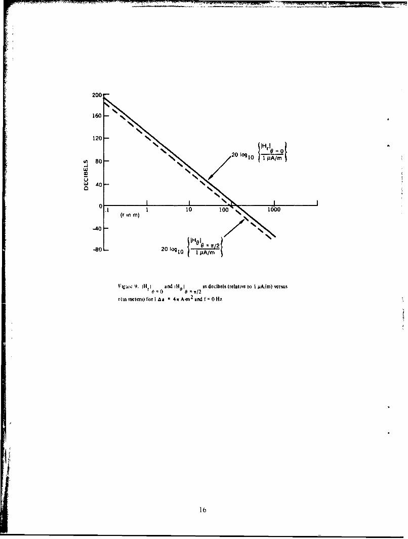
approximately the same potential as that of the seawater at a point just outside the skirnearest the ampulla end of the canal*. Therefore, the ampullary receptor acts like a voltagesensor (see Ref. 1, pp, 189-190), with the long canal enabling the seisory cells to sample theapplied voltage gradient at two widely separated points. Sharks ani ,kates have hundreds oithese canals, which are oriented in various directions and which rcach lertgths in skates of upto one-third of the body length (Ref. 3).

The magnitude of the voltage which is sensed by the sensory cells in the ampullae ofLorenzini, when an electric field is applied along the outside of the jelly-filled canal, is givenby:**

j E(r0'ds[ (I)

where V is the magnitude of the sensed voltage, d s is a differential distance directed alongthe canal's longitudinal axis; C represents a path of integratinn which is parallel to th.canal's longitudinal axis, lies completely in the body tissues which surround the canal, andextends from the ampulla to the surface pore: and E( -) is the electric field at the position ralong the path of integration, C., If the field E ( r ) is constant along the outside of the canaland parallel to the canal's longitudinal axis, then the integral in Erq. (1) yields:

V = 1EoI q (2)

where 1E01 is the amplitude of the constant electric field and Q is the length of the canal.Equation (2) suggests that if the lengths of the largest canals in kates or sharks are propor-tional to the body lenr hs of these fish, then the larger sharks and skates should be able todetect lower amplitudti hreshold electric fields, This is also suggested by Kalmijn (Ref. 4);however, he does not mention whether there was any difference between the longer andshorter skates used in his experiments (these skates (Raja clavata) varied from 30 to 60 cmin length) with regards to their responses to the lowest amplitude uniform electric fieldsapplied to these skates. (The applied electric fields in Kalmijn's experiment were 5-Hz squarewave fields, amplitude I uV/m zero-to-peak.) At present, no experimental evidence can befound which verifies this suggestion.

Although the ampullae of Lorenzini have been identified as the electroreceptors inskates and sharks, it has not been shown that structures of this type are responsible forpassive electroreception in all electroreceptive fish.. As pointed out by Bullock (Ref. 3),%. , we must not be surprised if some other types [of electroreceptors] turn up inaddition."

*The skin of sharks and skatzs has a low resistance, while the body tissues have a resistance which is much greater thanthe resistance of seawater Therefore, voltage gradients in the body tissues (,.e approximately the same as those externalto the fish (ReJ 1

*This formula is valid for the longer (anals when the applied electric fields are large-scale (i r generated by large plateelectrodes on either side of the fish, or, perhaps, generated by locali:ed sources which are at large distancev from the fishas comp.red to the physical dimensions of the fish) When the applied electric field is a local field (generated by nall,closely spaced electrodes placed near the fish), most of the voltage which is ensed by the sensory cells is developedacross the skin (Ref 1) In this report we will mainly be interested in large-scale applied electric fields

4

3. ELECFROMAGNETIC DIPOLE FIELDS IN THE OCEAN(NO BOUNDARY EFFECTS) AND THEIR

DETECtION BY SKATES

A. A BRIEF SUMMARY OF ELECTROMAGNETIC WAVE PROPAGATIONIN THE OCEAN*

Let us consider electric and magnetic dipole fields. Before writing out the dipolefields (which is done in subsections B and C), a brief summary is given of the equations fromwhich these fields are derived. Electromagnetic propagation in any media can always becharacterized by Maxwell's equations,

VXH = J +jw D (3)

V X E = -jw B (4)

V B =0 (5)

V.D p (6)

where,

E = electric field vector (Mm).H = magnetic field vectot (A/m)

D = electric displacement vector (coulombs/m 2 )

B = magnetic induction vector (webersim 2 )

J = Source current - density vector (Aim 2)

p = Source volume chaige density (coulombs/m 3) [See Eq. (7)]and

w = angular frequency of the monochromatic fields** (rad/sec)

Combining Eq. (6) with the divergence of Eq. (3) yields the equation of charge~continuity:

iV . J j~ (7)

The divergence of Eq. (4) yields Eq.. (5), and the divergence of Eq. (3) in conjunction withFq. (7) yields Eq. (6). Therefore, Eqs. (3) through (6) are not independent, and constitutive

*For a much more detailed summary, see Kratchman (Re! 5)"One may always obtain the arbitrary tme-varying fields from a superpositon (Fourier transform) of the monochromatic

fields in lintir media For a review of transient fields an conductive media, see Wait (Ref 6).

relations between the field vectors are needed., For a linear, isotropic medium these consti-tutive relations may be expressed as follows-

B = pH (8)

D = i"E (9)

where p is the complex magnetic permeability of the inedium (in henries/m), and i is thecomplex electric permittivity of the medium (in farads/m). For the ocean,

)A 4r X 10- 7 henries/m (10)

I -e-oo (I I)

where

e 80 oand 0 = 8.854 X 10-12 farads/m

and

a - 5 mhos/m (the conductivity of se.,water)

Combining Eqs. (3) (4). (8), and (Q) yield the wave equation which governs electro-magnetic propagation in the ocean:

V XV X E +Y2 E = -iw"AJ (12)

where,

3y = - o-p = -W2-pe+jW;A (13)

It is Eq. (12) from which the electromagnetic (EM) fields generated by any given sourcecurrent, J can be derived., In general, the EM field can be expressed as a sum of electric andmagnetic multipole fields* (dipole, quadrapole, etc.). In subsections B and C, only the elec-tric and magnetic dipole fields will be of interest, since the mathematical form of thesefields is simple and easy to compute plus the fact that dipole fields are good approximationsto the EM fields produced by the simplest (and most prevalent) types of antennas (loopsand straight wires).** For a good summary of FM fields gener-ated by different types ofsources in the ocean, see Refs. 5 and 6.

*See Papas (Ref 7), pp 97.108, or Chapter 16 of Jackson (Ref 8)

"The equation for electric or magnetic dipole fields Isee Lqs 125)-(27) and Lqs (30)-32J are valid or any straight wireor plane loop (whoe length or diarieier is sma!lr than a wavelength) carrying a constant current such that the fieliobservation distance from the wire or loop is much larger (at kast 5 times larger) than the length of the wire or theradius of the loop For observation distances which are clse to the current source, the geometry of the source cannot

be ignored

6

B. ELECTRIC DIPOLE FIELDS IN THE OCEAN

Electric dipole fields are generated by an elementary Hertzian dipole (a very short,straight wire caiying a constant current, 1). The electric dipole current which represents aHertzian dipole may be expressed mathematically as:

. ez lQ6(x)6(y)6(z) (14)

where e is a unit vector pointing in the z-direction; 2 is the dipole length, and 6(x) is theDirac delta function. (For a derivation of Eq. (14), see Ref. 9, pp. 6-8.) Equation (14)corresponds to an electric dipole pointing in the z-direction and located at the center of aCartesian coordinate system: (x, y, z). Solving Eq. (12) with J given by Eq. (14) yields theelectric dipole field components (in terms of a spherical coordinate system superimposedover the Cartesian coordinate system, so that z = rcosO)*.

Er = 1l/(joe+a)] (IlRcos0/2r 3)(I +r)e - 3' r (15)

EP I(j'e + o)(1 U QsinO/4w r3 ) ( +Yr + 7'2 r2) e-.r (16)

Ho = (I sin0/4v r2 ) (I +-yr) e-'r (17)

It is seen that for DC sources, w = 0, and the electric dipole field reduces to:

Er = (18)2wo r3

E = Qsin (19)4wo r3

Ho = I Q sinO/4w r- (20)

Notice that Ho is a factor of a larger, and decreases less with distance than Er or E0 for theDC case. For ly ri 1" 1, the far-zone EM field is given by (neglecting terms of l/(,yr) 2 and!/(-Yr) 3 ):,

Er 0 (21)

= . lsin0 yE0 =~A) J ,rr e - r (22) .E0 _ u I sin e-- r (22)

4rH IlkysinO .. y r (23)

Notice that in the far field:

IE0/H1 1 (l +j) (fora > oe) (24)

7

'7

The quantity

represents the characteristic impedance of the ocean to EM wave propagation. In the ocean,for a t we, note that Eqs. ( 15)417) can be written:

Er I rQCO (I +,r) e-r (25)

E0 I R sin 0(26)4-o (1 y-"r +y 2 r2 ) e - 'r (

H = q sin0 (i+ -fr)e"yr (27)

4w t

Where-, V jow = (1 +j)Vu/j72..* In Figs. 2 and 3, the functions 10 +yr) e-7r- B and Il + -yr + 2 r 2) e-3'r, = A are plotted.

*Throughout the rest of this report, it u assumed that -f (I +,) V viz. a> w e This is a good assumption in sea-water for frequencies less than 109 Hz (Ref 10)

DC level of B (-f =0)

0.8

Lj 0.6

0

C.4

0.2

00 1 2 3 4 5 6 7 8 9

2W

Figure 2. The function B I(I +,yr) er Is VS~ r.

8

1.5 -

1.2

DC level of A (y f 0)

0.9

-J 0.< 0.6

0.3 -

010 1 2 3 4 5 6 7 8 9

Figure 3. The functionA = Il( +yr +2T2),~veus rr .

In examining the possible detection of electric dipole fields by skates (threshold= I pV/r,, we are interested in the magnitudes lErI and 1EO I., In Fig. 4, lErI, IEo ,, andIH0 are plotted for f= 1 Hz.

In Fig. 5, lErl, lEo 1, and IH, I are plotted for f= 10 Hz. In Fig. 6, lEr1, 1EO 1, andI H I are plotted for DC fields.

In Figs. 4, 5, and 6.1I = 4 wo z 60 A-ne, This particular value for the currentmoment, 19, was chosen so that at I m

1E 010 = v/2 = IV/m

at DC (in seawater). It is seen in Figs. 4, 5, and 6, that for this particular value of Ik, both, , o1lo.=,

2

and

JEron = 0

reach the threshold level of skates in a very short distance (approximately 100 m for all

three cases - f 0, 1,10 Hz). It would require a tremendous current moment, 12, to make

9i

60 IH I0 2

20 1 PA/'40

20

0° 2 35

M -20 - r,

Figure 4 , Ir 1e 6 = 0'l el ,= and IHU Ie / in dccbels (relative tot I Vm or I MA/ml vs2

2OW r 0 r(in m)/22S) for IQ - 4o -, 60 A-m and f = 1 Hz.

the electric fields extend very far in the ocean., For instance, suppose the electric field

IE0 1t0 = r/2

were to reach a value of I pV/m at 1000 km for f= 0. This implies Ifrom Eq. (26)] that10-6 = I Q/(20 X 1018), or, IV - 6.3 X 1013 A-r. This would re4uire a current of 6.3 X1013 A in a wire I m long, or, equivalently, a current of I A in a wire 6.3 X I013 m long!For the DC electric field to reach a value of I pV/m at 1 km would still require a currentmoment of approximately 6 X 104 A-r. At either f = I Hz or f = 10 Hz, the required cur-rent moments for the electric dipole fields to reach a value of I pV/m at 1000 km and I kmwould be orders of magnitude greater than 6.3 X 1013 A-m and 6 X 104 A-m respectively,due to the presence of the exponential attenuation factor e-^tr in Eqs. (25)--27). It is

10

40 - 20 lOglo II A/rn

20

0-20

S-40

-60 2 3- 04

8020 lqgio A M -" --80-

Figure S. Ir0 1E8 I and IM I m decibels (relatwe to I uV/m or I MA/rn) versus

P0--2 r(=ronr)/71.4) forlV=4rn ft 60A-mandf = 10Hz.

noted that for a hypothetical "magnetic" fish sensitive to magnetic fields* of I A/m(0.001 gamma), it would be possible to sense the electric dipole field further away than foran electric field-sensing fish, For instance, at f = 0 Hz (Fig. 6), a "magnetic" fish couldsense an electric dipole field (for 1Q - 60 A-m) at 1 km. For f = 1 Hz (Fig. 4), this thresholddistance is approximately 900 m and for f = 10 Hz (Fig. 5), the threshold distance is approx-imately 380 m. Therefore, the sensing of electric dipole fields at extremely low frequencies(f 10 Hz) by the most sensitive electroreceptive fish known (Raja clavata) is limited torelatively short distanices (approximately 100 m for current moments on the order of 60A-m).,

*As pointed out by Kalmiln (Ref 1). electroreceptive fish could sense a magneti, field, B, by moving through the field at avelocity, v, which is perpendicular to B. This motion produces a potential gradient ofmagnitude Iv I1B 1, which the fishsenses Howe ver, the threshold level of the magnetic field which the most sensitive fish (threshold 7z 1 1A V/m) could meas-ure would be given by B = I emu,(100 cm/sec) = 0.01 gaus3 (assuming the fish could reach a velocity of 100 cm/sec)This value for the threshold level of the magnetic field is quite high (i e, 0.01 gauss is approximately 2 5% of the earth'smagnetic field), and an electroreceptive sish would be better off (in terms of detection distance) to directly sense theelectric part of the above-mentioned electromagnetic fields

Ii A

I;

200 -

120

80

, 100

-80 -

g r6. IE r 0 M 1 0EO10 and IN decibels (relative to I V/m or I A/m) vs

rInEq. (2, i fth aea 4 o tp 60 Aam and ol f 0 Hz

C. MAGNETIC DIPOLE FIELDS IN THE OCEAN

Magnetic dipole fields are generated by elementary loop currents (a very small planfloop carrying a constant current 1). The generating electric current of a magnetic dipolefield is given by (Ref. 9):

J_ = V x MO (28)

where,

M = ez IAa6(x)6(y)6(z) (29)In Eq. (29), A a is the area of the plane loop, and all other symbols are as defined in Eq.( 14). The positive normal to the plane loop current (defined by Eqs., (28) and (29)] isparallel to the z-axis. Solving Eq. (1 2) with J given by Eq, (28) yields the magnetic dipolefield components (in terms of the same coordinate system used in subsection h):

E0 - (l + yr) e--fr sinO (30)41 r

H, =" cos Ao'.' ~ A"'

V r3 0 +Yr) e-rcos01)

H0 = 2 2)_ a 7,H 4 r3 (0 +ara + r2) e-'rsino (32)

4W r

For DC currents, y 0, and the magnetic dipole reduces to:

E =0 (33)

' 1 A a cos0Hr = o(34). r 2 3

I; 2wr 3

H0 = 1 Aa sin(H 4rr3 (35)

It is rioted that the electric field vanishes for f =0. For 1'Yrl )t 1, the far-zone EM field isgiven by:

E jp 1&a sin 0 e- 7r (36)

Hr =0 (37)

-2H O A a sin0 e-Y' r (38)4w'r

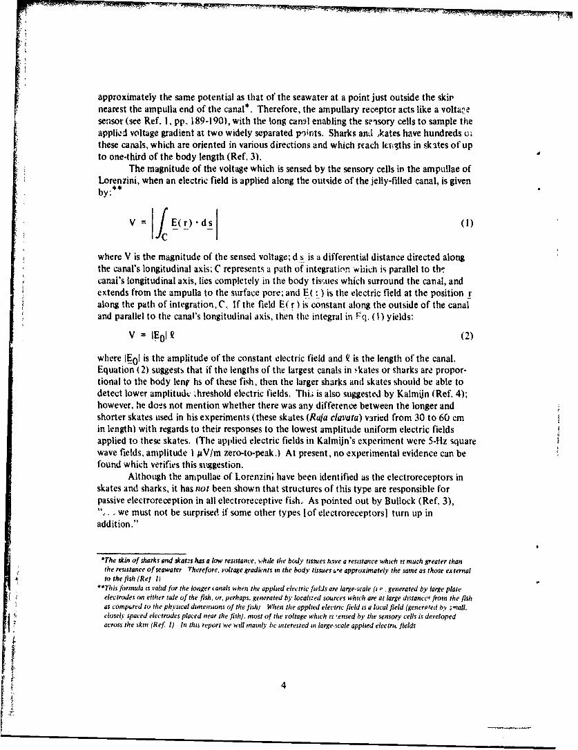
It is seen from Eqs. (3 1) and (32) that Hr and H0 for the magnetic dipole field is equivalentto Er and E0 for the electric dipole field (with I Aa replaced by 1/a)., In Fig. 7, 1E , IHr1,and IH0 Iare plotted for f = I Hz. In Fig. 8, IE I, IHrl, and IH0 I are plotted for f = 10 Hz.In Fig. 9, IHr and IH0 1 are plotted for DC fields (f= 0 Hz).

Note that in Figs. 7, 8, and 9, 1 Aa = 4irA-m2 12 A-m2 so that at r = I m (for DC)

1H01 0 = /2 = I A m-1.,

It is seen from these figures that for this particular value of I Aa, IE0I reaches the thresholdof skates in an incredibly short distance (approximately 2 m for f = 1 Hz and 7 m for f = 10Hz). * It is also seen that the magnetic fields (for I Aa - 12 A-m2 ) of magnetic dipoles fallotf in exactly the same way as do the electric fields of an electric dipole field (Figs. 4, 5, and6) as noted above. Therefore, a hypothetical "magnetic" fish which is sensitive to -i magnet-ic field of I MA/m (0.001 gamma) could detect magnetic dipole fields (f = 0, 1, 10 Hz and IAa - 12 A-m 2) out to approximately 100 m.

*A I DC, electric fish can still detect magnetic dipole fields by moving perpendicular to the DC magnetic field (as discussedpreviously). However, if the fish is sensitive to I V/in and can move at a velocity of I in/sec, it will only be able to de-tect the dc magnetic dipole field (I A a - 12 A-rn-) out to approxinately I m,

13

UAW r (r (in m)/225)

0 2

-40 -20 log10 Io H 0 1 /2

-60

-80

-100 -20 lag10 IPA/m

-120

-14 20 log 10 I1E Uv =/ A/

Figure 7. M~r H -, 0 af2,nd iE 01O=/ in decibels (relative to I MA/in or I MV/rn) vs.

e i r( rnm)1225)fCon Aa = 4wA-rn indf I lt.

14

40

20

r r (in m)/71.4)

01H 2 )-20 -20 log 10 lI1LjA/rn

-40

*~-60 -2 ol p/

-80 -0lg o I ,10 ,f/

-100-1A/

-120L

Figure 8. Ifd0 IN 0 2,and iE 01 o r2in decibels (relative to IuA/rn or 1 UV/m) versus

~j r Iinm:ters)/7l 41 for 1 43 4w Arn2 and f 10 Hz.

II ....

200-

160 -

120N

~~80 N ~ 20 log 0 liAr

U NW40-

. r 7- 1 10 100 N 1000(r inm)

-40 -

-80 20 log10 1______

, 9. IHt I0 0 and iHO I In decibels (relative to I uA/m) versusS0 os=w/2

rton meters) forI Aa 4w A-m2 and f 0 Hz

16

4. ELECTROMAGNETIC WAVES TRAVELING ALONG THE OCEAN'S SURFACEAND THE POSSIBILITY OF THEIR DETECTION BY SKATES

Asiue from the possibility of detecting electrical dipole fields which propagate di-rectly through the ocean, electroreceptive fish could, in principle, detect electrical dipole

*fields which are generated in the ocean and travel up to and along the ocean's surface andthen leak back down to the electric fish.,* This up-over-and-down mode of propagationwhich has been analyzed in detail with regard to submarine communication** is depictedgraphically in Fig. 10.

In this section this up-over-and-down mode of propagation of electrical signals willbe considered. It is possible that skates could detect electrical signals following such anindirect path since, as will be seen, signals following this path are exponentially attenuatedmuch less than signals following the direct path (through the ocean) from source to skate.

Presumably, electroreceptipe fish could also detect electric fields which travel along the ocean bottom. However, forbrcv ay, these fields will not be considered (For a study of electrical fields propagating along the ocean bottom, seeRef 11.)

"For a good review of submarine communication and the up.over.and.down mnode of electromagnetic propagation, seeRef. 12.

air

_., oroeanptiv

electroreceptive'1- f ish

dipole source

Figure 10. Up-over-and-down path of electric field propagation in the ocean.(Arrows indicate path of electric signal)

17

As a matter of fact. the exponential attenuation of electrical signals following the up-over-and-down path is given by e-1; o I see Eqs. (40)-42)1. where 6 =V/7i is the skin depth.

(which iF the depth in the ocean at which electromagnetic fields are reduced by approxi-mately 9 dB from their value at the surface) and D is the combined vertical depth of thedipole source and the skate. For f= I flz and 10 Hlz, exponential attenuation of approxi-mately 9 decibels will occur at D - 225 m and D - 70 m, respectively. Therefore, forskates near the surface (less than 50 f,), the dipole source at 1 Hz may be submerged to adepth of 700 ft (or 200 ft at 10 Hz) and only 9 dB exponential attenuation will result. [Ofcourse, inverse R2 and R3 losses (where R is the distance from the dipole source to the ray)will still be present. See Eqs. (40)-(42).] It is for this reason that the up-over-and-downpath o,' propagation is considered as a possible means of detection of dipole fields by elec-troreceptive fish. (For brevity and because a horizontal (parallel to the water's surface),electric dipole produces the strongest electromagnetic surface wave (see Ref. 9, pp. 232-235) only a horizontal electric dipole as the source of the electromagnetic field for theup-over-and-down path of propagation will be considered.)

Bailos (Ref. 9), in an excellent treatise on dipole radiation in the presence of a con-ducting half-space, has derived extremely useful approximations for the electromagneticfields generated by electric and magnetic dipoles submerged in a con ,...tiv halfspace.*The coordinate system used by Baios is a cylindrical coordinate syste, entered on theoc an's surface directly above the electric dipole (see Fig. 11). The horizontal, electricdipole current source is represented by:

I = ex!Q (x)6(y)6(z+h) (39)

where e.x is the unit vecor pointing in the x-direction, h is the depth of the dipole, and allother symbols are as defined in Eq. (14). The expressions for the electric field componentsin the ocean are given by (see Ief. 9, p. 209):

Ei 2wr 3 e-7) ( h1-z) (40)Elr 21ra r3 (0

E 1R sin ehz)(41)

Elz = I cos 0 _--h-z) (42)2,fr 2 a

For purposes of reference, the expression for the dominant z-component of the eleclricalfield in the air just above the ocean's surface will also be given:

E-Y _ )IQ cos 0 yE" 2Iror" - e 'h ef43)

As in Section 3, -y in the above formulas is given (to a very good approximation) by (I - j).

*Sonmnerfeld (Ref 13) was the first to consider dipole radiation near a conductie half-space.

18

ZIz!

air (2), p., eO0

hj

Oe.00 , - horizontal, electric dipole

r

electroreceptivef ish

(r, €z)

Figure II. Coordinate system showing the position of the source and the electroreceptive fish.Note that at the position of the electroreceptive fish, z < 0.

It i. very important to note the region of validity in which Eqs. (40)-(43) hold.First of all, the dipole source as well as the electroreceptive fish (skate) must be close to theocean-air interface, viz., the condition h,z < r, where r is the horizontal distance from thesource to the skate (see Fig. I I), must be satisfied. The condition W/c r < 1 < lJyri shouldalso be satisfied., This latter conditiot implies that the horizontal distance between sourceand skate exceeds several wavelengths in the conducting medium, but amounts to only asmall fraction of a free-space wavelength. Since free-space wavelengths at frequencies whichare of interest here (f <_ 10 Hz) are quite long (c/w > 5 X 106 m) and the ocean wavelengthsin this frequency range are quite short in comparison (I/ 1,'I 300 in), it is this region ofvalidity (which Bailos calls the "near-field region") which is of interest in this report. Actu-ally, the quasistatic region (0 < co/c r <I) is also important for our considerations; however,formulas valid in this region arc quite similar (see Ref. 9, Chapter 4). In any case, thenear-field formulas are quite useful in establishing an upper bound on the detection distancefor detecting submerged sourc,,s (via the up-over-and-down path) by electroreceptive fish (orany electrical sensor). Note that aside from the contributions to the electrical field given byEqs. (40)-(43), there are also contributions due to the effects of the ionosphere (see Ref.14). However, in the ranges of horizontal distance from source to skate which are impor-tant here, these ionospheric effects can be neglected.

19

In Fig. 12,

IElrI = 0' El01, r2' and IE2zy, 0

are plotted for f = I Hz and 10 Hz and 1 = 4ao it 60 A-m. Plots of

JElzj 0= 0

will not be included since this component of the electric field is negligibleI I EIz I20 l0gl0 <-1 20dB for both f- I Hz and 10Hzand r 1 m .

20 lg10 ljPV/m JmAlso, since Eqs. (40)-(43) are only valid for r > I/17 1, all plots will start at r - I/1,y1. InFig. 12, no exponential attenuation losses have been included, although these losses areeasily included by subtracting 9 dB per skin depth submersion from the levels shown for

E2z 10=0' Ilrl = 0 a d EI = r / "

0

10 100 )1000

2loo 1 f = 1Hz

-20 - 20 og 10 @f 1 Hz and 10 Hz

Figure 12 IE I IE .I , and tE2 i nm decibels (relative to 1 jV/m) versus

(in kilometers) forl 1 = 4iro 60 A-mn at f I | Hz and f = 10 Hz.

20

As can be seen from Fig. 12, for I R 60 A-in, the range of detection of a horizontalelectric dipole by the most sensitive skate (via the up-over-and-down path) is limited toapproximately 100 m, which is about the same range as for the direct path (see Figs. 4,5, and 6). Actually, 100 m is slightly outside the region of validity of the formulas [Eqs.(40443)A for f = I Hz, however, by using the formulas appropriate for the 100-n range(quasistatic formulas) one would still arrive at a value of approximately 100 m as the upperbound for detection by skates of electric dipoles via the up-over-and-down path at f = IHz. For the fields to extend much further than 100 m, incredible current moments areneeded. For instance, a current moment of approximately 6 X 1013 A-m is needed forthe dipole fields to be detected at 1000 km at either I Hz or 10 Hz. For detection at Ikin, a current moment of approximately 6 X 104 A-m would be required at either I Hzor 10 Hz. (Note that IE2zl, the normal electric field component in air, falls off less rapidlythan either lEj lor lEIrI, However, this component, )E2z I, is down to 1 pV/m at a hori-zontal distance of approximately 300 m for I f 60 A-m and f = 1 Hz or 10 Hz.) There-fore, the sensing of horizontal electric dipole fields via the up-over-and-down path of propa-gation at extremely low frequencies (f < 10 Hz) by the most sensitive electroreceptive fish(Rala clavata) is limited to short distances (approximately 100 m for current momentson the order of 60 A-in).

21

ii

21

5. A COMPARISON BETWEEN THE ELECTRIC-SENSING CAPABILITIES OFSKATES AND ARTIFICIAL SYSTEMS

In this section a comparison is given of the electric dipole sensing capabilities of askate (Raja clavata) with those of man-made systems with regard to the maximum detectiondistance (MDD) of a narrowband, extremely low-frequency (f < 10 Hz), electrical signalgenerated by an electrical dipole.* In particular, two different types of artificial systemswill be examined. The first. which is an underwater system, will consist of one electric fieldsensing antenna (a pair of highly conductive plates, a receiving toroid, etc.) which is con-nected to a sensor (bandpass fifter and voltage sensor). The second type of sensing systemconsidered consists of one sensing antenna which is placed above the ocean's suface.**This antenna is also assumed to be connected to a sensor.t The performance of these differ-ent types of artificial systems will be compared with the electric dipole sensing capabilitiesof a skate.

To make a comparison between these differt nt types of sensing systems (artificialand natural), a study must first be made of the noi,:3 fields in which these different systemsare found., The dominant component of the noise field surrounding sensing systems locatedabove the ocean's surface is the vertical component (perpendicular to the ocean's surface)and consists mainly of lightning noise (atmospherics) as well as noises of ionospheric origin.The extensive studies of atmospheric noise conducted in recent years (Refs. 16 ard ', 7) haveshown that in the range of frequencies of interest (f <, 10 Hz), the vertical compone .. ok theelectrical noise field was near 50 dB relative to 1 9IV/mA/H.t

In the ocean, sources of natural noise are much more numerous, and atmosphericnoises are not as dominant in the ocean as in air. The reason for this decrease in amplitudeof atmospheric noise is that in the ocean, the dominant component of the atmospheric noisefield is the tangential component, ta parallel to the ocean's surface. This component is;elated to the dominant vertical component of the noise ",eld just above the surface, Ealrvert'by the following relation (Ref. 14):

sea airEa 3.76 X 10- X6i E rt (44)tan vr

*The findings of Section 3 concerning magnetic field detection by electroreceptive fish make it unnecessary to compareartificial and natural sensing systems with regard to the detection of magnetic dipoles. Clearly, based on the most recentdata concerning measured thresholds of electroreceptive fish, artificial systems are far superior for purposes of magneticdipole detection Of course, one could obtain a reasonable estimate of the MDD of magnetic dipoles by artificial sys-tems by the use of the appropriate field formulas (see sect 3 or Ref. 9).The electric signal sou-ce for this type of sytem is presumed to be a horizontal, electric dipole submerged in the oceanat a depth not lower than one or two .xin depths.

tThe use of multielement sensing arrays will undoubtedly increase tie MDD of artificial systems. However, the analysis

of a single.element array should give a reasonable estimate of the lower beund on the MDD of artificial systems. For anexcellent review of multielement arrays, see (Ref. 15).This value did not vary a great deal for different locations )r times. It is assumed here that this noise level is fairly repre-sentative of noise levels over the sea at these frequencies. Of course, this assumption may not be valid, and more noisedata over the sea at extremely low frequencies is #aeeded.

23

For f 10 Hz, Eq. (44) indicates that in the ocean, atmospheric noise is down by at least100 dB from its levels in the air just above the ocean's surface. Actually, this figure of 100dB loss does not include the exponential attenuaticn e- /6 , where 6 = /27w3Ju and R is thedepth of noise penetration. However, at the low freqaencies we are considering, such atten-uation can be neglected down to depths of approximately 100 m since 8 70 m at 10 Hz.Of course, it is this exponential attenuation which blocks out atmospheric noise in theocean at frequencies greater than 100 Hz (Ref. 10).

Therefore, according to Eq. (44) and the data of Ref. 16, it is seen that in the ocean(within a skin depth of the ocean's surface) the tangential component of the atmosphericelectrical noise is approximately -50 dB relative to 1 MV/m/%/P" for f 5 10 Hz, This noiselevel seems to be of little consequence to the passive electric sensing system of skates. Ofcourse, there are other sources )f noise in the ocean. Kalmijn (Ref. 1), in an excellent re-view paper, has mentioned several sources of electrical noise which may influence electric-sensing systems in the ocean. Among the different types which are mentioned are noisefields due to ocean currents flowing through the earth's magnetic field (measured noisefields up to 50 pV/m); noise fields due to geomagnetic variations (measured noise fields onland up to 100 pV/m - measured noise fields in the ocean - in coastal waters and along thecontinental shelf - up to 10 pV/m), noise fields of electrochemical origin (no availabledata); and noise fields of biological origin., Indications are that due to the wide variety ofsuch noises, noise fields in the ocean might reach levels comparable to atmospheric noise inair. However, more measurements of electric field (as well as magnetic field) noise at vari-ous places in the ocean and at different times are needed.*

Therefore, due to the scarcity of noise data in the ocean, it will be assumed that thebackground noise in the ocean at extremely low frequencies consists mainly of atmosphericnoise at a level of -50 dB relative to I pV/mA/Hz. (Actually, this is probably a good as-sumption down to 5 Hz (see Ref. 10). From 0-5 Hz, the other sources of noise mentionedabove will most likely start to contribute to ocean noise**., At this point, it should benoted that if actual noise levels in the ocean are, indeed, much greater than -50 dB, then astudy of the signal processing capabilities of electrosensing fish might be needed (especiallyif the ocean noise levels were found to be much above 0 dB relative to I ,IV/m/V/R'z) for anadequate comparison between artificial and natural sensing systems. Of course, it is quitereasonable to assume that skates and electroreceptive fish in general have developed,through evolution, a very sophisticated signal processor which is quite capable of detectingextremely low frequency signals (bioelectric fields, for instance) in the presence of a greatdeal of noise.t

Based on the results of th-s report and the assumptions stated above, it is seen thatthe MDD of skates at frequencies below 10 Hz is approximately 100 m (see Sections 3B and4). (It is important to note that this value of 100 m corresponds to IR = 4vo 60 A-in.However, since we will assume a source current moment approximately 60 A-m for all sys-tems, this value is not too important since it is only a relative comparison between the artifi-cial and natural systems that is sought.) The MDD values of the two different artificial

*Lebermann (Pef 10) has reported some data on the spectrum of natural geomagnetic noises in the ocean.With regard to electric field noises in the S-80-Hz range off the coast of Baa California, see the article by Soderberg(Ref 18). Soderberg's data for depths between 30-300 m agrees (approximately) with the assumed value given above,i.e., -50 dB relative to I j V/m/'vI.

t'For the detection oJ signals by fresh water electroreceptve fish in the presence of lightning noise, see the article byHopkins (Rcf 19).

24

systems mentioned previously will now be compared with this value of 100 m for the skates.First to be considered is the artificial underwater system., As stated above, this systemconsists of an electric field sensing antenna connected to a bandpass filter and voltage sen-sor. The filter bandwidth will be assumed to be 1 Hz* and the sensitivity of the voltagesensor will be assumed to be approximately 10 nV. (This value of 10 nV sensitivity is ob-tainable with voltage sensors presently on the market. See Ref. 24.)

For the optimum design of this system, the noise level present in the system will beconsidered first. This noise consists mainly of the ocean noise which, as assumed above, ishorizontal to the ocean's surface and is at a level of -50 dB relative to I ,*V/m/v'Rz, or 3 X10- 9 V/m/vIE. Since the filter bandwidth is assumed to be I iz, it is seen that thesmallest electrical field signal which can be detected is 3 X l0- 9 V/m (assuming that thelowest possible filter output signal-to-noise ratio (SNR) for signal detection is l).

Assume now that the sensor system (filter plus voltage sensor) is connected to anelectric field sensing antenna (conducting plates, long wire, toroid, etc.) which is alignedparallel to the direction of the incoming electric field vector. Then, the magnitude of theopen-circuit voltage which is sensed by the voltage scnsor is given by v = I j-eff ' Ein c j,where 2 eff is the effective length of the antenna and Ei n c is the incoming electric field. It isnoted that the effective length of an antenna is not always the same as the antenna's actualphysical length. (See, for example, Chap. 4 of Ref. 25.) In general, an antenna's effectivelength depends on the frequency of operation, the external medium, etc.** By choosing asensing antenna with an appropriate effective length, one can detect an incident signal fieldof 3 X 10- 9 V/m and yet have the voltage signal at the input of the voltage sensor above its10-nV sensitivity. For instance, by connecting the sensor to an antenna with an effectivelength of approximately 3 m (f 10-8 V/3 X 10- 9 V/m), it is possible to detect an incidentsignal field of 3 X 10- 9 V/m, On the basis of Figs. 4, 5, and 6, this would correspond to anMDD of approximately 0.5 km at 1 Hz, and an MDD of approximately 0.4 km at 10 Hz.For detection of direct-path signals with I£ 60 A-m, see Fig. 13, As seen in Fig. 12, 3 X10-9 V/m corresponds to an MDD of approximately 1 km (for detection by the up-over-and-down path with I£ m 60 A-m and with the source electric dipole assumed to be horizon-tal (Fig. 14)i Therefore, from the above considerations, the MDD of the artificial systemdescribed above will be set at approximately 0.5 km for direct-path detection over the I - to10-Hz range.t When the electric dipole is approximately horizontal and the combineddepth of the dipole source and electric sensor is less than a skin depth, the MDD of thisunderwater system is 1 km for the indirect path detection over the I- to 10-Hz range. Of

*A fixed-bandpass filter with bandwidth 1 Hz is considered in this report for the sake of simplicity in the following com-parisons. Of course, other types of filters might be more desirable than the fixed.bandpass typ,. For instance, adaptive.type filters may be desired for their ability to track frequency drifts in the input signal. See, for example, Widrow (Ref20), Widrow, et al., (Ref. 21), Zeidler and Chabries (Ref. 22), and Griffiths (.Ref. 23).

*Swain (Ref 26) has shown that the effective length of a tuned toroid antenna in a conducting medium can be made verylong as compared to the physical dimensions of the toroid. By inserting a long, highly conducting core in the center ofr the toroid, its effective length can be made even longer (Ref. 27).

tBy submerging the sensing antenna at very great depths (greater than 3 skin depths), ocean noise will be reduced at thevoltage sensor input (at least in the 5. to 10-Hz range) due to exponential attenuation as noted previously. Therefore,the MDD of the underwater system will be raised somewhat over the 0.5-km value given above just by lowering the sys.tem deeper in the ocean. However, the MDD value will not be raised by very much because of the exponential attenua-tion of the signals. Therefore, the 0 5.km value for the MDD for direct-path detection is a reasonable estimate.

25

air

i ocean

noise t3 X 10- VlmI-V/"z

sensor (bandpass filter and voltage sensor)

h > 3 skin depths

00 sensing antenna (plates, wire,toroid, etc.) aligned parallel

4,0 to electric dipole

*~Q*

electricdipole

Figure 13. Direct-path detection alignment for underwater system for f a 1-10 Hz (not drawn to mcale).

course, these MDD values are probably somewhat optimistic since the ocean noise fields aremost likely more intense than the assumed level (3 X 10-9 V/mk/z/T'z), at least in the 0- to5-Hz frequency range.

The second type of artificial sensing system (for detecting horizontal electric di-poles) to be considered consists of a single sensing antenna placed above the ocean's surface.,Once again, it is assumed that the antenna is connected to the sensing system describedabove. In this case, the vertical component of the electric noise field (just above the ocean'ssurface) is 50 dB above I pV/rmnAz as noted above, or, equivalently, 3 X 10 -4 V/mk/V/,and the horizontal component of the electric noise field (just above the ocean's surface) is 3X 10-9 V/m/Vql. Using a magnetic field sensing antenna as well as an electric field sensingantenna in this system is also a possibility. In this regard it is noted that the horizontalcomponent of the magnetic noise field just above the ocean's surface in the extremely low-frequency range (f < 10 Hz) is approximately l0-6 A!m/H/ir (Ref. 16). Since the filterbandwidth considered in this report is 1 Hz, it is noted that the smallest vertical electricalfield signal which can be detected (for output SNR of 1) is 3 X l04 V/m, which is about300 times greater than the skate threshold. The smallest detectable horizontal electric fieldsignal is 3 X l0- 9 V/m and the smallest detectable horizontal magnetic field signal is l0-6

A/m.A vertical electric field, horizontal electric field, or horizontal magnetic field at these

magnitudes Q X 10-4 V/in, 3 X 10-9 V/n and 10-6 A/m, respectively) can be

26

- MDD I km for 12 9 60 A-m-

air noise 3 X 10 - V/m//Hoceall i ..... .01 ' OI 1 ' . . . "

xn :l io3 1 V/m/vHsensing antenna (plates, sensorwi-e, toroid, etc.) alignedparallel to the electricdipole (perpendicular to thesurface of the paper)

h < 1-2 skin depths

t horizontal electric.,,,--'dipole (perpendicular to the

surface of the paper)

Figure 14. Indirect.path dctection alignment for underwatt-r system for f 1-10 Hz (not drawn to scale).

detected by the sensor system connected to an electric field sensing antenna or a magneticfield sensing antenna. A vertical electric field sensing antenna with an effective length ofless than I m can be used to detect the vertical component of electric fields on the order of3 X 10

"4 V/r., Referring to Fig. 12, we see that the MDD of this system with a verticalelectric field sensing antenaa (for source depth not greater than a skin depth) is less than 0. 1km for 1 - 60 A-m and for f= 1-10 Hz. By analogy with the underwater system, the MDDof this system with a horizontal electric field sensing antenna placed just above the ocean'ssurface is approximately 1 km. Use of a magnetic field sensing antenna (a loop will beconsidered) will increase the MDD of this system somewhat. From Ref. 28, it can be seenthat the magnitude of the voltage sensed by a core-loaded loop is given by V = pe W Hinc.

AN, where Hinc is the magniti-de of the incident magnetic field; A is the area of the loop; Nis the number of turns of wire in the loop;, and pe = p Or/(l + D (pr - 1 )), where pr is the*relative permeability of the core and D is a dimensionless parameter related to the shape ofthe core (D = 0 for long thin cores; D = 1/3 for spherical cores; and D = I for cores in theshape of thin disks). From this formula it can be seen that a loop with an area of. I m2 and10 turns loaded with a long thin core (D 0 0) of high permeability (Mr ~ 100) could sense avoltage of approximately 10 nV for an incident horizontal magnetic field of magnitude 10- 6

A/m at 1-10 Hz.

ir = 41 X IO- 7 henries/m.

27

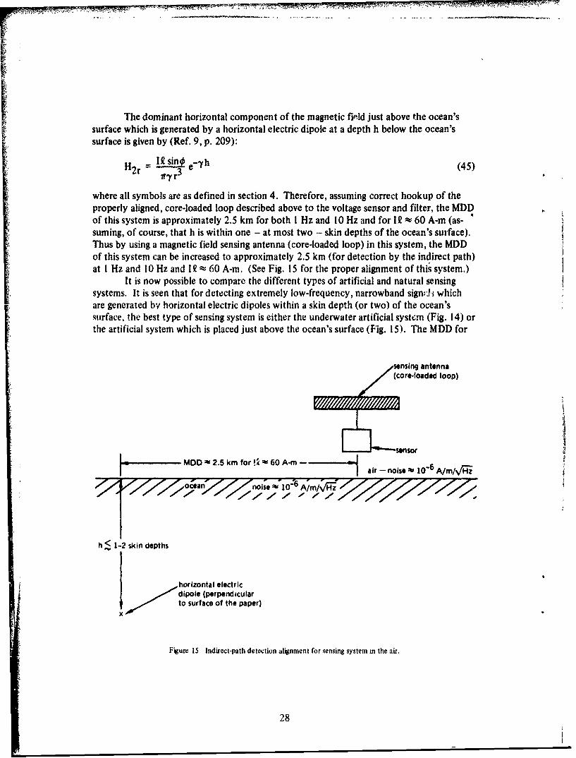
The dominant horizontal component of the magnetic field just above the ocean'ssurface which is generated by a horizontal electric dipole at a depth h below the ocean'ssurface is given by (Ref. 9, p. 209):

H2r = IQ sinO e-h (45)

where all symbols are as defined in section 4. Therefore, assuming correct hookup of theproperly aligned, core-loaded loop described above to the voltage sensor and filter, the MDDof this system is approximately 2.5 km for both 1 Hz and 10 Hz and for IQ f 60 A-m (as-suming, of course, that h is within one - at most two - skin depths of the ocean's surface).Thus by using a magnetic field sensing antenna (core-loaded loop) in this system, the MDDof this system can be increased to approximately 2.5 km (for detection by the indirect path)at 1 Hz and 10 Hz and 12 - 60 A-m. (See Fig. 15 for the proper alignment of this system.)

It is now possible to compare the different types of artificial and natural sensingsystems. It is seen that for detecting extremely low-frequency, narrowband sign:,! whichare generated b', horizontal electric dipoles within a skin depth (or two) of the ocean'ssurface, the best type of sensing system is either the underwater artificial system (Fig. 14) orthe artificial system which is placed just above the ocean's surface (Fig. 15). The MDD for

sen antenna(core-loaded loop)

E sensor

MDD : 2.5 km for !k v 60 A-m --air -noise 106 A/m/Vr

h 1-2 skin depths

horizontal electricdipOle (perpendicularto surface of the paper)

Figure 15 Indirect-path detection alignment for sensing system in the air.

28

MWII

either system is approximately 2.5 km* (for I2 . 60 A-m and f= 1-10 Hz) which is approx-imately 25 times better than the MDD of a skate (Raja clavata) ( 100 m also at I C 60A-m and f = !-10 Hz). For detecting signals generated by sources deeply submerged in theocean (greater than 2-3 skin depths), the best type of sensing system is the artificial under-water sensing system (Fig. 13) with an MDD of approximately 0.5 km (for 12 60 A-m andf= 1-10 Hz) as compared to 100 m (also at I - 60 A-m and f= 1-10 Hz) for the skate.Therefore, man-made systems seem to be superior for the long-range detection of narrow-band, extremely low-frequency signals.

Of course, it should be pointed out that in this section, no restrictions were placedon the effective length of the antennas used in the man-made system (viz., we have chosenantennas with effective lengths of 3 meters), whereas the effective length of the skate'santenna is restricted to its maximum ampullary canal length, which is approximately 20 cm(Ref. 29). Therefore, it could be argued that the above comparisons are not fair and that tomake a better comparison, the effective lengths of the man-made antennas should be re-stricted to approximately 20 cm. However, what was desired in this section was a compari-son between the optimum, single-element man-made system and the optimum biologicalsystem (i.e., the skate). Therefore, no restrictions -'ere placed on the effective length of theantenna used in the man-made system. In fact, the only factor which limits the effectivelength is noise (atmospheric noise, etc.). The results of this section show that man-madesystems can sense down to the level of electric field noise in the ocean, while the optimumbiological system is apparently not this sensitive (see page 24). Even if a comparison be-tween the sensitivity of the optimum biological system and a man-made system of compara-ble effective iength (20 cm) had been desired, the man-made system would still have faredbetter than the skate (viz., the sensitivity of the man-made system with a 20-cm antenna isapproximately 10 nV/0.2m = 5 X 10-8 V/m, as compared to 10- 6 V/m sensitivity for theskate).

The above conclusions concerning the apparent superiority of man-made systemsover the skate are not too surprising when one considers that the passive electrosensing ofelectroreceptive fish in the ocean (especially the botiom feeders) is designed mainly for thedetection of very short-range bioelectric fields which emanate from prey that may be buriedin the sand. It is not important to the electroreceptive fish to detect an electric"I signalmany miles away, only at a very short range. Of course, more data are needed on the elec-tric field thresholds of clectroreceptive fish of different species, sizes, shapes, etc. New datamight indicate that electrosensing fish could detect electric objects at much greater distancesthan indicated in this report.

'Actually, accordug to the above analysis, the AIDD oj the underwater system consisting of an electric field sensing atten-na placed just below the ocean's surface is approximately one-half the MDD of the sensing system placed just above theocean's surface which employs a magnetic field sensing antenna. However, by using a magnetic field sensing antenna for"he underwater sensing system, the MDD o1 this svstet'i wi!! be exactly the same as the MDD of th"' .enmig i.vtem placedtbove the ocean 's surface (based on our assumptions concerning noise)

2)9j

6. (ONCLUSIONS

SUMMARY

In this report the possibility of the detection ofl dipole fields by electrosensing fishhi, been considered. In part icular, a skate (laja clarata) which is sensitive to thresholdelectric lields of I MV/m has been examined. This value represents the highest electrical,-,nsitivity known in aquatic anim als. The results, presented in Sections 3 and 4, indicatethat skates detect electric dipole fields (either by the direct path of propagation through thewaitcr (Section 3) or by the tip-over-and-down path of propagation (Section 4) at relativelyshort distances (approxinately 100 mi at f= 0, I . or 10 Hz and for source current momentsoi the order of' 00 A-in). As pointed out in Section 3. electrosensing fish can also detect theelectric field component of a magnetic dipole source as well as the magnetic field compo-nents of both magnetic and electric dipole sources (by moving relative to the magneticiCIds), but detection of these con ponents is limited to very short ranges (approximately

7 In tfor either magneti,. dipole moments of 47r A-m 2 or electric dipole moments of approxi-mately 60 A-ni at f= 0, 1, and 10 lIz).

In Section 5, a comparison is made between the electric dipole sensing capabilities ofskates and artificial systems. In particular, two different types of artificial sensing systemswere considered. The first was a system for underwater use and the second was a sensingsystenl to be used over the ocean's surface for detecting electric dipole sources submerged atdepths not greater than one or two skin depths. It was found that for purposes of detectingelectric dipoles submerged deep in the ocean (at depths greater than two or three skindeptils), the best type of' sensing system is the artificial underwater sensing system. Forelectric dipoles submerged at depths which are less than one or two skin depths, the besttype of sensing system is the artificial system that is placed either just above the ocean'ssurface or just below the ocean's surface. Of course, the conclusions reached above aresubject to certain assumptions, which are explicitlystated in Section 5. It is hoped thatthese considerations in Section 5 will provide a reasonable estimate of the lower bound onthe'1naximum detection distance of electric dipoles by artificial systems.

SUGGESTIONS FOR FURTHER WORK

It is rather clear that much more work needs to be done in the area of electromag-netic sensing by electroreceptive fish (or perhaps "magnetic" fish). Some of the areas forfututre work, as suggested by this report, include the study of magnetic-sensing capabilitiesofdifferent types of aquatic animals. Measurements of the effects of magnetic fields onbiological systems in general have been initiated (see, for instance, Ref. 30), however, meas-urements of magnetic thresholds of aquatic animals are not quite as numerous. As pointedout in Section 3, hypothetical "magnetic" fish sensitive to magnetic fields of I gA/n (0.001

31

PAU BL1.. .#±?*D i

gamma)*, could sense electric dipole fields further away than electric st:ising fish sensitiveto I AV/m. However, to determine if fish are sensitive to variations as .mall as fractions ofgammas in a constant background magnetic field of 0.5 gauss would require incredible ex-perimental accuracy. First. all background noises would have to be cancelled, and then aconstant background field of 0.5 gauss in addition to a well controlled, very small-amplitudemagnetic field (on the order of gammas or less) would be applied to the fish. Unfortunate- ,ly, t te big problem arises when one tries to shield out small-amplitude, magnetic-noise fluc-tuations. The cheaper magnetic shields effectively block out magnetic noise variations onlydown to tens of gammas in a relatively small volume. As an example, Helmholtz coils canreduce the magnetic field over a control volume of about 100 cc to less than t50 gammas.The cost of reducing magnetic noise fields to the order of gammas or less (over relativelylarge volumes > 1 m3 ) can become quite prohibitive., Therefore, shielding costs are so highthat low-amplitude magnetic-threshold measurements on aquatic animals are quite expensive.,

Another area for future work is the continued measurements of the electric fieldthresholds of electrosensing fish., Specifically, measurements of electric field sensitivities ofsharks and pkates of different lengths should be undertaken to dete"'nine whether longerelectroreceptive fish are, as suggested by Kalmijn (Ref., 1), indeed more sensitive. Suchmeasurements could be extremely useful as a further check on our models of passive electro-reception by sharks and skates. Of course, as mentioned in Section 5, more data on theelectric field thresholds of electric fish of different species are also needed. Finally, theneed for further measurements of electromagnetic noise occurring in the ocean is men-tioned. Indications are that at certain points in the ocean, electromagnetic noise might bequite larger than the lowest thresholds of skates, I pV/m (see Section 5)., Such measure-ments, therefore, could possibly aid in our understanding of the degree of signal processingwhich occurs in certain electric fish. This knowledgz might be of use in the design of artifi-cial signal processors.

This report has treated, mainly, passive electrosensing fish. Of course, electrogenicfish also exist (Ref. 2), i.e., fish capable of creating their own electric field for the purposesof detecting objects and communicating with other fish. A quantitative look at the electricfields produced by these fish as well as the distortions in these fields which are caused byobjects placed in the fields might be of use in the design of artificial active electromagneticsensing systems for use either in fresh water or in the ocean.,

*Quite properly, these hypothetical fish would be sensitive to magnetic field variations of 0.001 gamma within the earth'sbackground magnetic field (- 0.5 gauss)

32

77,

REFERENCES

1. A. J. Kalmijn, "The Detection of Electric Fields from Inanimate and Animate Sourc-es Other than Electric Organs", chap. 5 in Handbook of Sensory Physiology III, A.Fessard, ed. New York: Springer-Verlag, 1974.

2. H. Scheich and T. H. Bullock, "The Detection of Electric Fields from Electric Or-gans", chap. 6 in Handbook of Sensory Physiology III, A. Fessard, ed. New York:Springer-Verlag, 1974.

3. T. H. Bullock, "Seeing the world through a new sense: electroreception in fish",American Scientist, vol. 61, May 1973, pp. 316-325.

4. A. J., Kalmijn, "The electric sense of sharks and rays", J. Exp. Biol. (1971), 55,pp. 271-383.

5. M. B. Kraichman, Handbook of Electromagnetic Propagation in Conducting Media,NAVMAT P-2302, Headquarters Naval Material Command,. 1970.

6., J. R. Wait, "Electromagnetic Fields of Sources in Lossy Media," in Antenna Theory,Part I1, R. E. Collin and F. J. Zucker, ed., PP. 438-514, McGraw-Hill, New York,1969.

7, C. H. Papas, Theory of Electromagnetic Wave Propagation, McGraw-Hill, New York,1965.

8. J, D. Jackson, Classical Electrodynamics, John Wiley & Sons, Inc., New York, 1962.

9, A. Batlos, Dipole Radiation In the Presence of Conducting Half-Space, PergamonPress, Oxford, 1966.

10. L. N. Liebermann, "Other electromagnetic radiation", in The Sea, M. N, Hill, ed.,vol. 1, pp. 469-475, Wiley, New York, 1962.

11. H. Mott and A., W. Biggs, "Very-Low-Frequency propagation below the bottom ofthe sea", IEEE Transactions, vol. AP-11, No. 3, May 1963, pp. 323-329,

12. R. K. Moore, "Radio Communication in the Sea," IEEE Spectrum, Nov., 1967,pp.42-51.

13. A. Sommerfeld, "Uber die Ausbreitung der Wellen in eber drahtiosen Telegraphie,"Ann. Physik 28, 665-737, 1909,

14. W, L. A nderson, "The Fields of Electric Dipoles in Sea Water - the Earth-Air-Ionosphere Problem," Tech, Rept., EE-88, Engineer. Expt. Station, Univ. of NewMexico; Albuquerque, New Mexico, May, 1963.

33

15. A. A. Ksienski, "Signal-Processing Antennas," in Antenna Theory, Part II, R. E.Collin and F. J. Zucker, eds., pp. 580-654, McGraw-Hill, New York, 1969.

16. E. L. Maxwell and D. L. Stone, "Natual noise fields from I cps to 100 kc", IEEETransactions, vol. AP-! I, No. 3, May 1963, pp. 339-343.

17. "World Distribution and Characteristics of Atmospheric Radio Noise", CCIR Rept.322, Documents of the Xth Plenary Assembly, Geneva, 1963. Published by Interna-tional Telecommunications Union, Geneva, 1964.

18. E. -F. Soderberg, "ELF noise in the sea at depths frum 30 to 300 meters", J., ofGeophysical Res., 74, 2376-2387, (1969).

19. C. D. Hopkins, "Lightning as background noise for communication among electricfish", Nature (London), vol. 242, pp. 268-270 (1973).

20. B. Widrow, "Adaptive Filters", In: Aspects of Network and System Theory, R. E.Kalman and N. Deelaris, edb., Holt, Rhinehart & Winston, Inc., New York, 1971.

2 1. B. Widrow, J. R. Glover, J. McCool, et al., "Adaptive Noise Cancelling: Principlesand Applications," IEEE Proc. Vol. 63, No. 12, Dec. 1975, pp. 1692-1716.

22. Naval Undersea Center, NUC TN 1476, An Analysis of the LMS Adaptive Filter usedas a Spectral Line Enhancer, by J, R. Zeidler, D. M. Chabries, Feb. 1975.

23. L. J. Griffiths, "Rapid Measurement of Digital Instantaneous Frequency", IEEETransactions, Vol. ASSP-23, No. 2, April 1975, pp. 207-222.

24. Teledyne Crystalonic Data Sheet for C413N Silicon Epitaxial Junction N-ChannelField Effect Transistor. Available from:., Teledyne Crystalonics:' 2082 S.E. Bristol St..Suite #4, Newport Beach, CA 92707.

25. Antenna Theory, Part 1. R. E. Collin and F. J. Zucker, eds., McGraw-Hill, New York,1969.,

26. G., R. Swain, "A Small Magnetic Toroid Antenna Embedded in a Highly ConductingHalf-Space", J. Res. NBS, Vol.. 69D, No. 4, (1965), pp. 659-665.

27. R. H. Williams, R. D. Kelly, and W. T. Cowan, "Small Prolate Spheroidal Antenna ina Dissipative Medium," J. Res. NBS, Vol. 69D, No. 7, (1965), pp. 1005-10 10.

28., W. L. Weeks, Antenna Engineering, McGraw-Hill, New York, 1968.

29., Private communication with E. 1. Knudsen, Scripps Institution of Oceanography,

30. Biological Effects of Magnetic Fields, Vol. 1I, M. F. Barnothy, ed., Plenum Press,New York, 1969.

34