Electromagnetic Boundary Layer Control

Daniel Sura

2

EMBC Report - Table of Contents

1.0 Introduction to the MHD experiment 3

2.0 Background 5

2.1 Theoretical 52.2 Experimental 9

3.0 Test Setup and Hardware Design 133.1 Baseplate/cassette redesign 133.2 Assembly of MHD hardware 193.3 Electronics 23

4.0 Results 25

4.1 Magnetic and electric field mapping 254.2 Boundary layer measurements 31 4.2.1 Boundary Layer data 31 4.2.2 Comparisons to prior work 354.3 Force Measurements 36 4.3.1 Background (Jan 2003 measurements) 36 4.3.2 Drag force measurements, drag contour 38 4.3.3 Force time trace data 44

5.0 Conclusions 46

References 49

6.0 Appendix 50

6.1 Force Time Series Case 1: 0 m/s 52 Case 2: 1.5 m/s 56 Case 3: 3.0 m/s 67 Case 1: 0 m/s log 75 Case 2: 1.5 m/s log 80 Case 3: 1.5 m/s log 89

6.3 Electronic component schematics 97

3

1.0 Introduction

Over the past several years, experimental work has been conducted in pursuit of

validating predicted drag reduction from numerical simulations developed by engineers

and scientists working in the hydrodynamics field. Some techniques developed in the past

few years have demonstrated drag reduction and have validated some of the theories and

simulations of drag behavior in fluid flow over a surface. Drag reduction technologies

such as the injection of micro-bubbles into the boundary layer, the use of riblets, and

electromagnetic forces to alter the boundary layer characteristics over a surface are prime

examples of research experiments conducted in recent years at various institutions.

Professor Karniadakis of Brown University’s Center for Fluid Mechanics and visiting

professor in the department of Ocean Engineering at Massachusetts Institute of

Technology has developed numerical simulations that predict drag reduction by

implementing a Lorentz force crosswise to the flow of fluid thereby altering the flow

behavior of near wall turbulent structures. The consequence of altering the

characteristics of the near wall turbulent structures, at an optimum predicted crosswise

forcing magnitude and frequency of oscillation, is drag reduction on the order of 30%

predicted by numerical simulations.

The impact of drag reduction technology capable of reducing drag that amount would

be tremendous to the ocean technology field. Shipping industries would certainly be one

of the first to take advantage of this type of technology. Any reduction in drag is directly

associated with a reduction in fuel consumption as well as the ability for a ship or marine

vessel to travel at higher speeds. In its current development of higher speed surface and

underwater marine vessels, the Navy is another institution that would greatly benefit from

the usage of this type of drag reduction technology.

4

Figure 1.1 3d Solid Model of the baseplate andcassette installed in the water tunnel test section

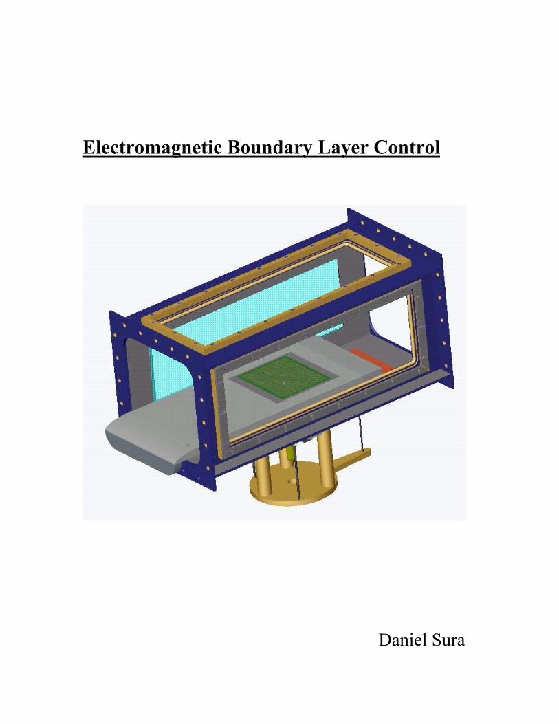
The experimental validation of numerical simulations of drag reduction due to Lorentz

force excitation was performed in the Marine Hydrodynamics Laboratory at

Massachusetts Institute of Technology. A flat plate made of white delrin plastic with an

elliptical nose shape was designed and built to be tested in a water tunnel test section.

Figure 1.1 shows a 3d solid model assembly of the flat plate in the test section. Notice a

square cassette with an integrated electrode board, which upon proper installation sits

flush with the delrin cassette and base plate. In the cassette are rows of integrated

magnets underneath the electrode board.

A Lorentz force is generated by the crossing of an electric field by current being

pumped through the electrodes of the electrode board, with a magnetic field produced by

magnets sitting in the cassette underneath the electrode board and in between the

electrodes. The design and setup of the hardware and electronics for this experiment, as

well as numerical simulation work, and results from experimental work performed at the

Marine Hydrodynamics Laboratory, will be discussed in greater detail throughout the

following sections of this report.

5

2.0 Background

2.1 Theoretical

Brown University’s Center for Fluid Mechanics has developed numerical simulations

that predict drag reduction due to the effect of altering near wall turbulent structures by

generation of a Lorentz force. To discuss the effects of the Lorentz forcing in the flow of

fluid over a flat plate, it is first necessary to understand the principles of how Lorentz

forces are generated in a fluid. A Lorentz force is a direct result of electric and magnetic

fields crossing each other and creating a force which is perpendicular to both of the fields

where they intersect.

Figure 2.1.1 Diagram of a Lorentz Force Model [1]

Figure 2.1.1 shows an illustration of electric fields crossing magnetic fields creating a

perpendicular force, which is the Lorentz force and is labeled ‘F’. Changing the

electrode size, (parameter a in the figure) will have an effect on the magnitude of the electric

field generated. An electric field is generated in a fluid that is conductive by using an

6

electrode board which has long strips of electrodes. Since the fluid is conductive, the

electric field is created from electrons traveling through the fluid from positive to

negative charged electrodes. Any change in the electric field magnitude will result in a

direct change in the magnitude of the Lorentz force. The following equation shows how

the Lorentz force is dependent on the magnitudes of both the electric

and magnetic field, Jo being the magnitude of the electric field, and Bo being the

magnitude of the magnetic field, as well as ‘a’, electrode size, and ‘y’, the distance in the

vertical direction away from the surface of the electrode board. As one may expect the

Lorentz force decays exponentially as the distance away from the surface of the electrode

board increases. The implementation of hardware and electronic components capable of

generating Lorentz forces for experimental work will be discussed in section 2.2.

Figure 2.1.2 Hairpin Vortex Production near a flat plate [1]

Experimental analysis, numerical simulations, and theory have shown that in fluid

flow over a flat plate, hairpin vortices are produced in and near the boundary layer.

Figure 2.1.2 shows an illustration of such vortices formed near the surface of the flat

plate where fluid is flowing in the +X direction. The production of near wall turbulent

structures result in regions of higher surface velocity and is a characteristic behavior in

flow past a flat plate. High surface velocity regions cause the formation of these hairpin

7

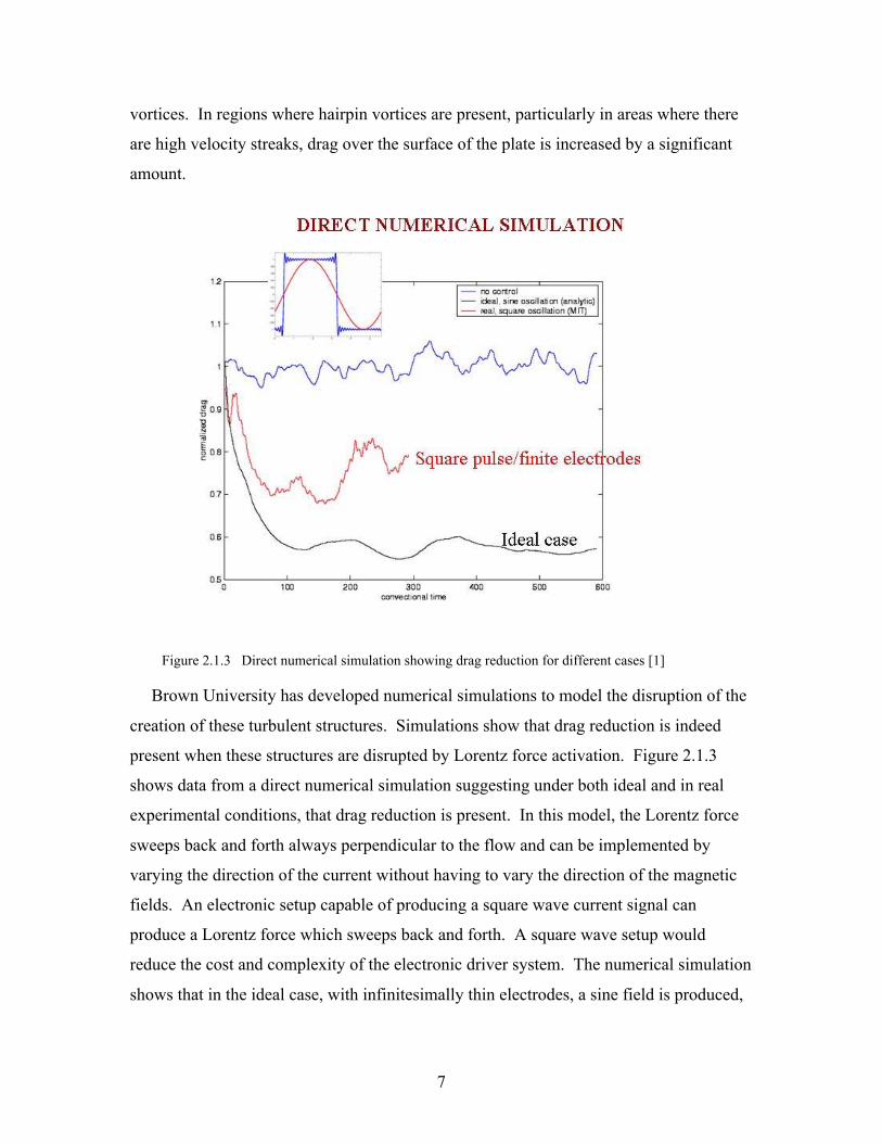
vortices. In regions where hairpin vortices are present, particularly in areas where there

are high velocity streaks, drag over the surface of the plate is increased by a significant

amount.

Figure 2.1.3 Direct numerical simulation showing drag reduction for different cases [1]

Brown University has developed numerical simulations to model the disruption of the

creation of these turbulent structures. Simulations show that drag reduction is indeed

present when these structures are disrupted by Lorentz force activation. Figure 2.1.3

shows data from a direct numerical simulation suggesting under both ideal and in real

experimental conditions, that drag reduction is present. In this model, the Lorentz force

sweeps back and forth always perpendicular to the flow and can be implemented by

varying the direction of the current without having to vary the direction of the magnetic

fields. An electronic setup capable of producing a square wave current signal can

produce a Lorentz force which sweeps back and forth. A square wave setup would

reduce the cost and complexity of the electronic driver system. The numerical simulation

shows that in the ideal case, with infinitesimally thin electrodes, a sine field is produced,

8

and the drag reduction is greatest. A square wave oscillation, which was used in the

experimental validation process, still results in drag reduction.

Figure 2.1.5 Numerical Simulation the baseline case leading to drag reduction [1]

A baseline case performed by the numerical simulations shows elimination of wall

streaks, indicating that wall turbulent structures have been disrupted. Figure 2.1.5 shows

a plot of predicted drag under no control and under Lorentz force disruption of the flow.

Simulations indicate drag reduction of up to 30% is possible under these conditions. The

baseline case was performed with an invariant parameter of 1, a forcing period of 50, and

a penetration depth of 1/50. The simulations have predicted that those parameters will

result in the maximum drag reduction for the square wave case. The validation of these

drag reduction predictions was the next phase of this research project and involved

experimental analysis conducted at the MIT water tunnel in 2002.

9

2.2 Experimental

Experimental work to validate the predicted drag reduction from numerical

simulations was performed in the Marine Hydrodynamics Laboratory by MIT alumni

Jaskolski in the fall and spring of 2001-2002 [2]. The hardware for the experimental

setup consisted of a flat base plate machined out of white delrin plastic with a

thickness of 1.5 inches, a length of 42.5 inches, and a width of 19.875 inches. Figure

2.2.1 shows a 3d solid model of the MHD (magneto-hydrodynamic) base plate as

well as the electrode board which is an integrated part of the plate after its

installation. The length of the base plate was designed to be 42.5 inches, long enough

so that the flow over the long flat surface would produce near wall turbulent

structures over the electrode board where Lorentz forces were generated and drag

force measured. An elliptical nose was designed so as to create a smooth transition

between flow moving over the lower wall of the water tunnel test section and over the

flat delrin plate.

Figure 2.2.1 Flat plate hardware for Jaskolski’s boundary layer experiment

The generation of a magnetic field was accomplished by having strips of magnets

underneath and between the electrodes of the electrode board. The electrodes of the

electrode board are 1/8th inches wide and are spaced apart 1/8th inches. The magnets

are also 1/8th inches thick and generate magnetic fields of up to 0.15 Tesla at the

10

surface of the electrode board which is exposed to the flow of water. If the fluid is

conductive, current can travel from electrode to electrode in the fluid, in a plus to

minus manner, and an electric field is generated.

Custom built driver electronics built by Jaskolski were connected to a power

supply capable of generating up to 166 Amps of current and a frequency generator

capable of outputting a square wave signal. The driver electronics allowed the

current to switch directions by changing the polarity of the incoming current from the

power supply. The resulting system was capable of producing square wave current

signals with variable amplitude and frequency. The output of the electronic driver

system was connected to the electrode board and a Lorentz force which switched

back and forth in the crosswise flow direction could be produced with varying

amplitude and frequency.

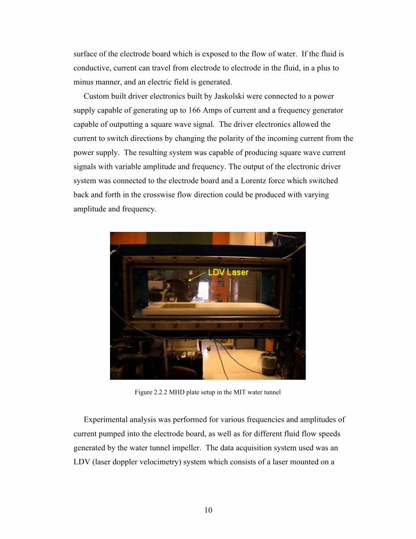
Figure 2.2.2 MHD plate setup in the MIT water tunnel

Experimental analysis was performed for various frequencies and amplitudes of

current pumped into the electrode board, as well as for different fluid flow speeds

generated by the water tunnel impeller. The data acquisition system used was an

LDV (laser doppler velocimetry) system which consists of a laser mounted on a

11

traverse system. The LDV system in the marine hydrodynamics laboratory can detect

particles of fluid moving in the flow and can accurately measure the flow speed in the

horizontal and vertical directions. The laser shoots four beams into the test section

window and into the flow, and the velocity measurement can be conducted where

these beams intersect. The traverse system has a resolution of 0.01 mm and can

accurately move to a desired position. Figure 2.2.2 shows a photograph of the MHD

base plate installed in the water tunnel test section. Notice the positioning of the

LDV laser and the electrode board installed in the MHD base plate. The hardware

was setup in the test section, so that boundary layer profiles could easily be measured

since the laser had the ability of taking measurements very close to the surface of the

flat plate and of the electrode board.

Figure 2.2.3 LDV data measurements performed by Corey Jaskolski – 2002 [2]

Boundary layer velocity profiles using Laser Doppler Velocimetry were measured for

various frequencies and current amplitudes. At the optimum predicted forcing frequency

of T+=100 by numerical simulations [1], the current was varied and velocity profiles

measured yielded the local shear stress at the wall. The changes in the local shear stress

are indicative of changes in drag. Figure 2.2.3 shows data

measurements of the changes in du/dy as a function of current amplitude for both a tunnel

flow speed of 1.5 and 3.0 m/s. The data clearly shows that a change in du/dy of about

12

26% is present at a current amplitude of 20 Amps for the 1.5 m/s second case, and at 40

Amps, the change in du/dy is -35%. This 35% change in du/dy agrees roughly with the

predictions by numerical simulations of 30% drag reduction. Although the local changes

in du/dy clearly show drag reduction locally, it is very difficult to make conclusions

about drag reduction on a global scale for the entire surface area of the electrode board.

Some of the boundary layer profiles measured showed increase in drag in some areas

over the electrode board, primarily over the electrodes themselves, and drag reduction in

between the electrodes [2]. To make conclusions about drag reduction on a global scale

with solely LDV acquired data would be inadequate. In pursuit of characterizing the

global drag effects by Lorentz forcing in the fluid, implementation of a force

measurement experiment to measure the global drag forces acting over the entire

electrode board was carried out in the Marine Hydrodynamics Laboratory.

13

3.0 Test Setup and Hardware Design

3.1 Base plate/Cassette redesign

In preparation for the next round of experimental work, with the objective of

quantifying global drag reduction, a major redesign of hardware and electronics was

carried out in the spring of 2002 at the Marine Hydrodynamics Laboratory at MIT. The

hardware redesign involved using the existing MHD baseplate, magnets, and the

electrode board from previous work conducted by Jaskolski [2]. It was determined that

the best method of measuring global drag force was to use load cells for a direct

measurement of force. This could be accomplished by creating a square cutout in the

MHD base plate, and having a square plastic delrin cassette which contained the rows of

magnets and the integrated electrode board. The electrode board was mounted by four

flat head screws on the corners, and a small 4-40 bolt in the center to keep the center of

the board from bowing upwards and affecting the flow.

Figure 3.1.1 Solid model of magnet and electrode board assembly

14

The rows of magnets were positioned in such a manner that all the magnets of one row

had the same orientation upwards, such as north, and adjacent rows would have magnets

which were oriented south so as to create a magnetic field from row to row. Figure 3.1.1

shows a 3d model of how the magnets are placed into the slots. The magnet filled

cassette sits flush with the MHD base plate and inside of the square cutout without

touching any of the edges of the cutout but having a small clearance of about 0.005

inches around all four edges. Figure 3.1.2 shows a 3d solid model of the MHD base plate

and the magnet filled delrin cassette.

Figure 3.1.2 MHD base plate and cassette 3d solid assembly model

The cassette was designed to be 14 inches long and 14 inches wide with a thickness of

0.687 inches and with a _ inch thick steel plate mounted on the bottom which touches all

of the rows of magnets and prevents any magnetic flux leakage from underneath the

cassette. An adapter shaft attached served the purpose of fitting and clamping into the

collet of a dynamometer which has integrated load cells for force measurements. The

dynamometer was available in the lab and has been extensively used for measuring the

drag and lift on hydrodynamic bodies such as hydrofoils. The assembly of the newly

designed base plate, cassette, and dynamometer in the test section will be discussed

further in section 3.2.

15

The design of new hardware for the upcoming experiment also involved the addition

of a dam made of delrin plastic on the leading edge of the MHD plate and a rear

extension block to cover the mounting hardware which extended past the rear of the

MHD plate. Figure 3.1.3 shows the assembly of the MHD plate with the addition of the

dam and the extension piece in the rear. The addition of the dam in the front, blocks the

flow of water so that none of it can enter underneath the MHD plate and affect the

mounting hardware and more importantly the shaft connected to the cassette which

mounts into the dynamometer. If the flow of water underneath the MHD plate were not

blocked, there would be flow induced vibrations on the shaft, and the load cells would

measure these effects and give us inaccurate readings for drag force and side force. The

extension block in the rear is not of critical importance but it was designed to reduce

flow effects coming from objects other than the flat plate itself nearby the electrode board

where sweeping Lorentz forces were generated.

Figure 3.1.3 MHD Plate Assembly with Non Magnetic Cassette

16

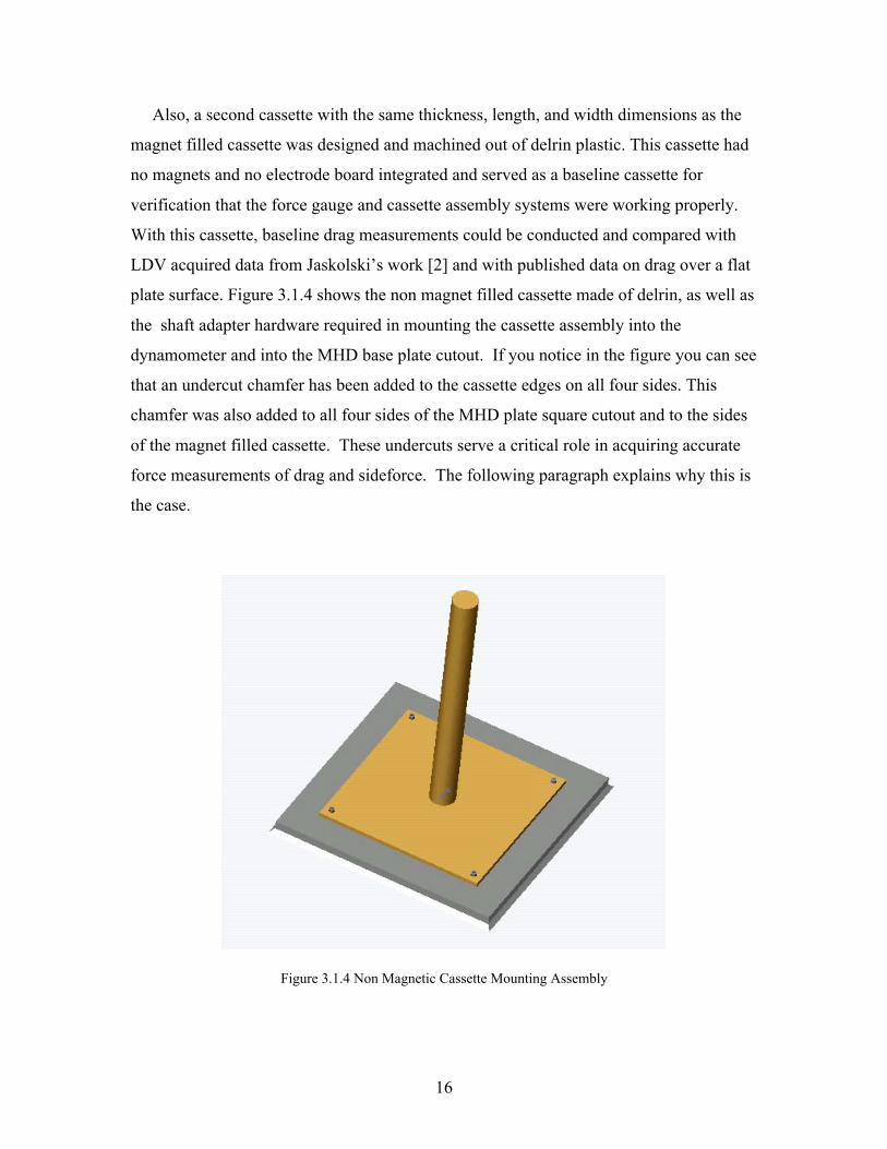
Also, a second cassette with the same thickness, length, and width dimensions as the

magnet filled cassette was designed and machined out of delrin plastic. This cassette had

no magnets and no electrode board integrated and served as a baseline cassette for

verification that the force gauge and cassette assembly systems were working properly.

With this cassette, baseline drag measurements could be conducted and compared with

LDV acquired data from Jaskolski’s work [2] and with published data on drag over a flat

plate surface. Figure 3.1.4 shows the non magnet filled cassette made of delrin, as well as

the shaft adapter hardware required in mounting the cassette assembly into the

dynamometer and into the MHD base plate cutout. If you notice in the figure you can see

that an undercut chamfer has been added to the cassette edges on all four sides. This

chamfer was also added to all four sides of the MHD plate square cutout and to the sides

of the magnet filled cassette. These undercuts serve a critical role in acquiring accurate

force measurements of drag and sideforce. The following paragraph explains why this is

the case.

Figure 3.1.4 Non Magnetic Cassette Mounting Assembly

17

It is difficult to position the cassette exactly in the center of the cutout in the MHD

plate, however it can be done to within a reasonable tolerance. This involves adjusting

the position of the cassette with respect to the shaft adapter hardware. Since the location

of the mounting hardware cannot be changed due to the shaft fitting into the

dynamometer collet, the hardware has slots where it bolts to the underside of the cassette,

allowing the adjustment of the cassette position, a process which can be very tedious and

time consuming. Even so, it is likely there will be a small gap difference between the

sides of the cassette and the MHD plate and the size difference depends on how

accurately the cassette was centered. Figure 3.1.5 shows a cross section of the cassette

mounted inside of the MHD plate cutout. The difference in gap at points A and B creates

a difference in pressure along the cassette caused by water flowing through the gaps and

acting on the side surfaces. This creates a force wanting to pull the cassette towards the

direction of the bigger gap, towards the left in the figure. This force is significant enough

to cause an effect on the force measurements measured by the load cells in the

dynamometer.

Figure 3.1.5 MHD Plate and Cassette Cross Section before undercuts

One solution to this problem would be to center the cassette exactly but this would

require spending a lot of time getting it as accurate as possible. A more adequate solution

to this problem was to add a chamfer to both the MHD plate and the cassette so as to

create a sharp point on the edges of all four sides of the cassette and the base plate.

Figure 3.1.6 illustrates a cross sectional view of the cassette installed inside of the base

plate cutout with the undercut chamfers. The addition of these chamfers eliminates the

18

induced force caused by the gap differences at points A and B. If there is a gap

difference at point A and B, the amount of area that is affected by the pressure in between

the gaps is minimized to that of a knife edge allowing the force to be small and

negligible.

Figure 3.1.6 MHD & Cassette Cross Section after undercuts

19

3.2 Assembly of MHD Components & Water Tunnel Description

The hardware for the force measurement experiment consists of an assembly of

components such as the magnet filled cassette and shaft adapter assembly, the MHD base

plate, hardware for base plate to dynamometer window mounting, the dynamometer

itself, and the load cells integrated into the isolation arm of the dynamometer. Figure

3.2.1 shows a 3D model, underside view of the dynamometer installed in the bottom of

the water tunnel test section. Notice three load cells colored in darker grey which attach

to the isolation arm of the dynamometer. The isolation arm is attached by thin rods at

three points to the rest of the dynamometer.

Figure 3.2.1 3D model of underside view of dynamometer, base plate, and cassette assembly

In this configuration, the load cells measure forces that are felt only by the isolation

arm which has a collet with a 1.5 inch diameter hole where the shaft from the cassette is

inserted and clamped with bolts. Figure 3.2.1 shows an exploded view of the cassette and

20

shaft aligned but not inserted into the collet of the dynamometer. The cassette shaft is

inserted into the isolation arm, and the load cells are directly measuring forces felt by the

cassette. The load cell used for the drag measurement was a 5 lb gauge and for side force

a 20 lb gauge.

The dynamometer has the capability of rotating to a desired angle, but for the force

measurement experiment, it was aligned perfectly parallel with the sides of the tunnel so

that the load cell measuring drag would measure a force which was exactly in the

direction of the flow, and load cell measuring side force would measure a force in the

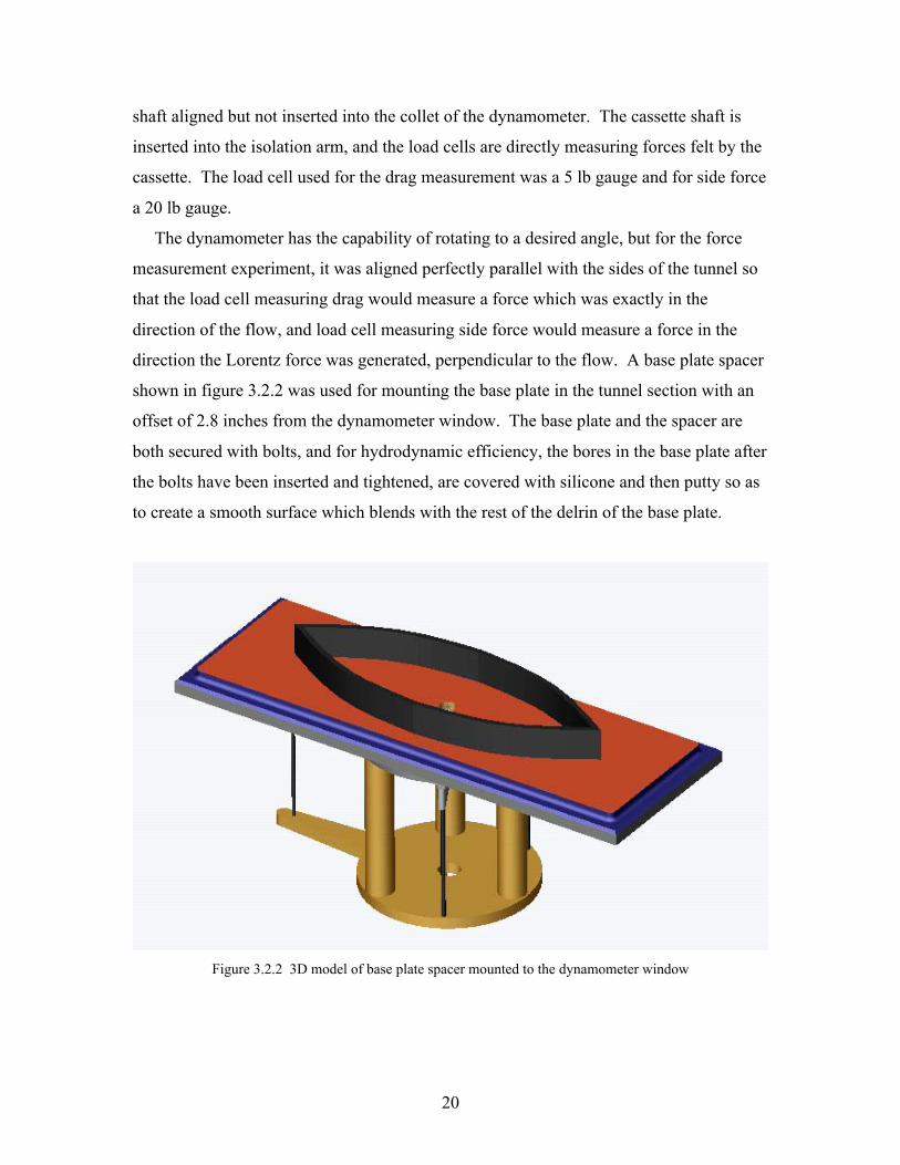
direction the Lorentz force was generated, perpendicular to the flow. A base plate spacer

shown in figure 3.2.2 was used for mounting the base plate in the tunnel section with an

offset of 2.8 inches from the dynamometer window. The base plate and the spacer are

both secured with bolts, and for hydrodynamic efficiency, the bores in the base plate after

the bolts have been inserted and tightened, are covered with silicone and then putty so as

to create a smooth surface which blends with the rest of the delrin of the base plate.

Figure 3.2.2 3D model of base plate spacer mounted to the dynamometer window

21

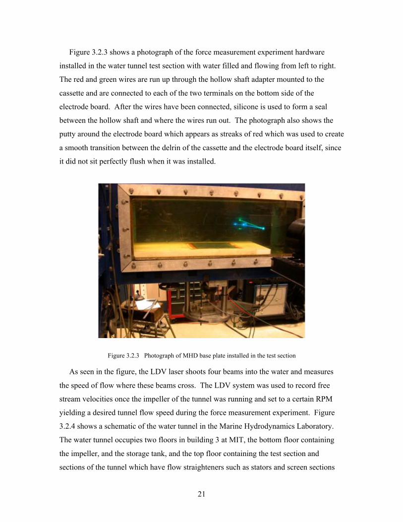
Figure 3.2.3 shows a photograph of the force measurement experiment hardware

installed in the water tunnel test section with water filled and flowing from left to right.

The red and green wires are run up through the hollow shaft adapter mounted to the

cassette and are connected to each of the two terminals on the bottom side of the

electrode board. After the wires have been connected, silicone is used to form a seal

between the hollow shaft and where the wires run out. The photograph also shows the

putty around the electrode board which appears as streaks of red which was used to create

a smooth transition between the delrin of the cassette and the electrode board itself, since

it did not sit perfectly flush when it was installed.

Figure 3.2.3 Photograph of MHD base plate installed in the test section

As seen in the figure, the LDV laser shoots four beams into the water and measures

the speed of flow where these beams cross. The LDV system was used to record free

stream velocities once the impeller of the tunnel was running and set to a certain RPM

yielding a desired tunnel flow speed during the force measurement experiment. Figure

3.2.4 shows a schematic of the water tunnel in the Marine Hydrodynamics Laboratory.

The water tunnel occupies two floors in building 3 at MIT, the bottom floor containing

the impeller, and the storage tank, and the top floor containing the test section and

sections of the tunnel which have flow straighteners such as stators and screen sections

22

which act to reduce turbulence in the free stream flow. The free stream turbulence of the

tunnel is on the order of 3% - 5% and design work is in progress for the installation of a

turbulence reduction mesh section capable of reducing the free stream turbulence to 1%

or less.

Figure 3.2.4 Schematic of MHL Water Tunnel

23

3.3 Electronics

Lorentz force activation requires the generation and crossing of magnetic and electric

fields. The magnetic fields were created by installing rows of magnets an 1/8th of an inch

apart and integrating them into the cassette just below the electrode board. To create an

electric field in the flow, current needs to be pumped through the electrodes of the

electrode board. The transmission path for current flow is through wires connecting the

outputs of four MOSFET’s (connected to a power supply and driver electronics) to the

electrode terminals located on the bottom of the electrode board.

Figure 3.3.1 The main electronic components for Lorentz force activation

In order to verify maximum drag reduction predicted by numerical simulations, the

current direction must be switched back and forth, with a magnitude that switches from

plus to minus and minus to plus, thus creating a Lorentz force which alternates in

crosswise flow direction from right to left and left to right. The amount of drag reduction

observed is a function of the frequency and amplitude of the Lorentz force and to validate

such effects, a requirement in the design of the electronics system was the capability of

being able to produce an adjustable current signal with a desired frequency and

amplitude. Figure 3.3.1 shows a photograph of the main electronic components required

24

in generating Lorentz force activation. The function generator serves the role of

generating a square wave signal and has adjustable frequency and an output which is

connected to the input of the driver electronics circuitry box.

For our new round of force measurement experiments Hydro Technologies of

Severance Colorado, upgraded the electronic gate driver circuitry used in Jaskolski’s

Lorentz force activated measurements. The new driver electronics contain a Schmidt

trigger, a high frequency driver chip, and other electronic components such as capacitors,

resistors, and power supplies. To power the driver electronics, a DC regulated power

supply capable of producing 15 volts was needed. The newly designed electronic

circuitry components allowed current polarity to be switched at a frequency of up to

several hundred hertz. The old circuitry worked reliably up to only about 120 Hz.

Because power supplies are not capable of producing wave forms with a frequency

greater than a few hertz, an h-bridge type switch was needed to produce the desired wave

form from a DC current output from the power supply used. The outputs of this circuitry

were connected to the gates of four MOSFET’s, which were then connected to the

outputs of the main power supply capable of generating 166 amps of current and to the

wires connecting to the terminals of the electrode board. The outputs of the driver

circuitry were connected in such a manner that they would open and close the gates of the

MOSFET’s repeatedly, thus changing the polarities of the two wires which connected to

the electrode board and allowing the generation of a square wave current signal which

alternated from plus to minus and minus to plus. Schematics of the electronics can be

found in the Appendix section.

25

4.0 Results

4.1 Magnetic and Electric Field Mapping

Magnetic and electric field mapping were performed in an effort to verify that both the

electric fields and magnetic fields were present over the electrode board in order to

produce Lorentz force activation. The magnetic flux was measured using a gauss probe

meter and was mounted to the LDV laser traverse so that positions for desired probe

location could be programmed and data acquired for various points across and above the

surface of the electrode board. Figure 4.1.1 shows a photograph of the major components

used in the magnetic field mapping as well as the coordinate system used.

Figure 4.1.1 Photograph of components used in magnetic flux measurements

The magnet filled cassette was set on top of a cart and delrin bars, and was aligned

with the probe so that movement of the probe would be perpendicular or parallel to the

rows of magnets and electrodes. Each of the magnets that make up the rows in between

the electrodes are 0.5 Tesla magnets, and the polarities in the rows alternate. For example

26

one row will contain magnets that are all oriented south and the two adjacent rows will

contain magnets oriented north.

Figure 4.1.2 Plot of magnetic flux vs x position over electrode board

Figure 4.1.2 shows a plot of the magnetic flux as a function of position x. Notice from

the plot that the maximum and minimum readings are 0.15 and

-0.15 Tesla. The probe position was setup so that x = 0 was the edge of the electrode

board which stuck out past the rows of magnets, thus no flux is present until an x position

of about 42 mm. At values of x = 56 mm and x = 68mm, the peaks are positive with

magnitudes of 0.15 Tesla. These are locations of the centers of rows of magnets oriented

north, and at x = 50 and x = 63 mm the peaks are negative with magnitudes of -0.15 Tesla

and are centers of rows of magnets oriented south. The widths of the magnets are 3.1

mm and the spacing in between rows is also 3.1 mm. Also notice from the plot that the

maximum magnitude measured at the surface of the electrode board was +/- 0.15 Tesla.

Although the cassette was filled with rows of 0.5 Tesla magnets, the probe was

27

measuring very close to the surface of the electrode board but at a distance of 0.06 inches

above the actual surface of the magnet rows. This distance above the magnet rows is

equivalent to the thickness of the electrode board

A similar verification process was carried out to verify that current was being pumped

into the electrodes of the electrode board. This test was a rather simple one since it

involved measuring voltage at the terminals where the wires connected and supplied

current coming from the power supply and driver electronics. A voltmeter was sufficient

enough to carry out this procedure. This test was performed on a spare electrode board

since it needed to be submerged in conductive water and it would have been difficult to

perform this procedure with the electrode board installed in the cassette and in the water

tunnel.

Figure 4.1.3 Photograph of voltage mapping experimental setup

Figure 4.1.3 shows a photograph of the test bed setup which had water filled half way

and with the electrode board submersed. Salt was added to the water to make it

28

conductive so electric fields could be created in the fluid at the surface of the electrode

board. In the water tunnel, roughly 800 lbs of sodium nitrite was added for 6000 gallons

of water in order to create conductive properties equal to half of sea water conductivity

which is in the range of 4.29 siemens/m [3]. The current output of the power supply was

set to 30 Amps and the function generator output was set to 20Hz and various voltages at

positions along the electrodes of the electrode board were measured with the voltmeter.

Figure 4.1.4 Diagram of voltage mapping layout

Figure 4.1.4 shows a diagram of the mapping layout where voltages were measured.

Three sweeps were made at locations of X = -4.25, 0, and 4.25 inches. At these X

locations 10 evenly spaced points from Y = -6.05 to Y = 6.05 inches were measured.

These measurements were made on two electrode boards, one of them was a previously

used board and had electrodes with widths of 1/8 inches and 1/8 inch spacing and the

other board was a brand new electrode board which had electrodes with widths of 1/16

29

inches and an electrode spacing of 1/8th inches. Figure 4.1.5 shows plots of the three

different X locations of voltage as a function of y position along the electrode board. At

X = -4.25 there is almost no variation in voltage along the Y axis, but for X = 0 and X =

4.25 the variation around Y = - 3 inches is significant and is due to the electrodes in that

region being corroded as well as the presence of epoxy which was accidentally spilt from

some other experimental work occurring in the lab.

Y [in]

Vo

ltag

e[V

]

-5 0 50

1

2

3

4

5X=-4.25X=0X=4.25

Thick Electroboard Voltage MapFrequency = 20 Hz, Current = 30 AIncoming Voltage = 2.772 V

Epoxy & Corrosion on board inthis area for x = 4.25, x = 0

Figure 4.1.5 Thick electrode board voltage mapping plot

This same test was also conducted on a new electrode board with thinner electrode

widths in order to verify that the variation seen in the thick electrode board was in fact

due to corrosion and effects of the epoxy. Figure 4.1.6 shows plots of the voltages as a

function of y position for the sweeps at the three different X positions. This data shows

no variations such as those that were found in the thick electrode board containing those

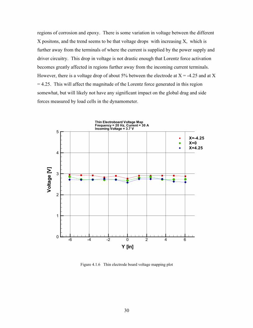
30

regions of corrosion and epoxy. There is some variation in voltage between the different

X positons, and the trend seems to be that voltage drops with increasing X, which is

further away from the terminals of where the current is supplied by the power supply and

driver circuitry. This drop in voltage is not drastic enough that Lorentz force activation

becomes greatly affected in regions further away from the incoming current terminals.

However, there is a voltage drop of about 5% between the electrode at X = -4.25 and at X

= 4.25. This will affect the magnitude of the Lorentz force generated in this region

somewhat, but will likely not have any significant impact on the global drag and side

forces measured by load cells in the dynamometer.

Y [in]

Vo

ltag

e[V

]

-6 -4 -2 0 2 4 60

1

2

3

4

5

X=-4.25X=0X=4.25

Thin Electroboard Voltage MapFrequency = 20 Hz, Current = 30 AIncoming Voltage = 3.7 V

Figure 4.1.6 Thin electrode board voltage mapping plot

31

4.2 Boundary layer measurements

4.2.1 Boundary layer data

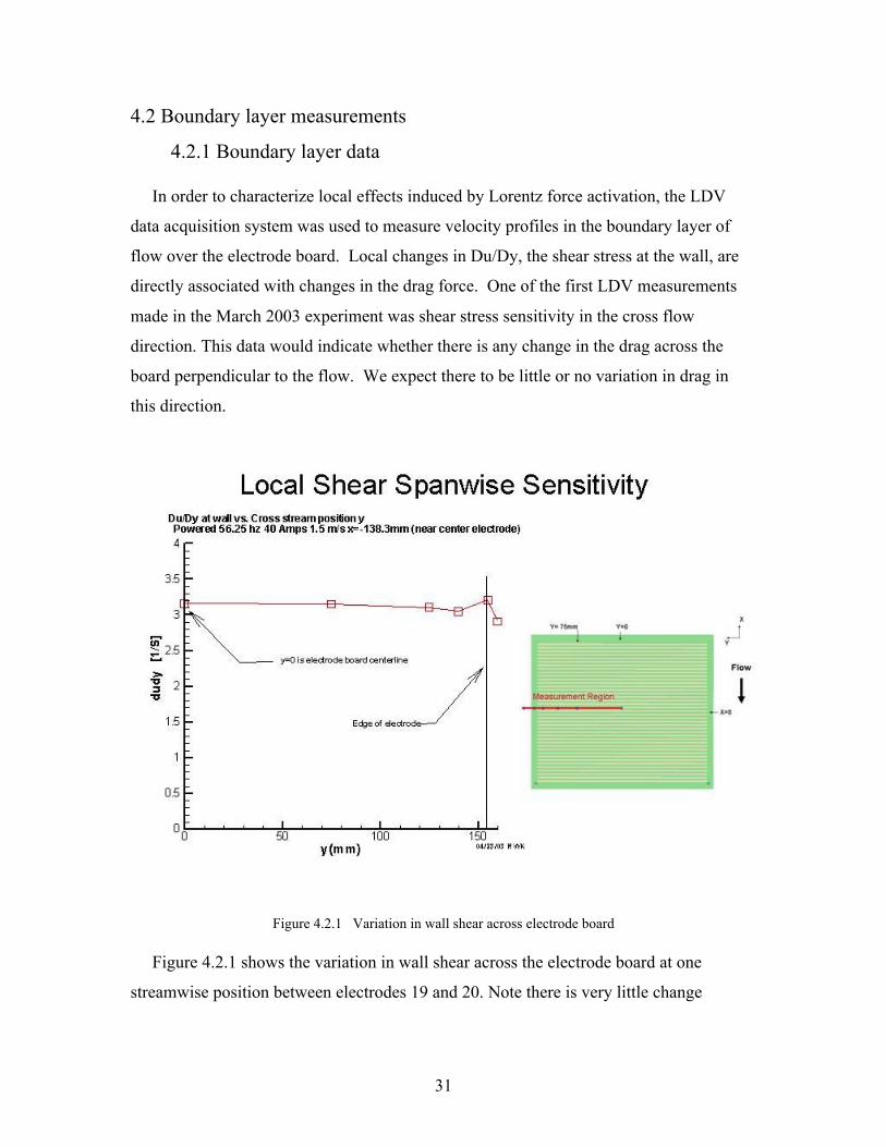
In order to characterize local effects induced by Lorentz force activation, the LDV

data acquisition system was used to measure velocity profiles in the boundary layer of

flow over the electrode board. Local changes in Du/Dy, the shear stress at the wall, are

directly associated with changes in the drag force. One of the first LDV measurements

made in the March 2003 experiment was shear stress sensitivity in the cross flow

direction. This data would indicate whether there is any change in the drag across the

board perpendicular to the flow. We expect there to be little or no variation in drag in

this direction.

Figure 4.2.1 Variation in wall shear across electrode board

Figure 4.2.1 shows the variation in wall shear across the electrode board at one

streamwise position between electrodes 19 and 20. Note there is very little change

32

from the centerline of the board all the way to the edge of the electrodes, thus validating

the off center measurements (y = 75mm) of most of the LDV measurements performed

later in March 2003.

Figure 4.2.2 Plot of variation in shear over electode spacing

Measurements in variation of shear over an electrode spacing in the flow direction

were also conducted. Figure 4.2.2 shows the variation in wall shear over the actual extent

of an electrode spacing. Three cases are shown, one with the cassette with the electrode

board but no magnets, another with the entire electromagnetic cassette unpowered, and

the last with the electromagnetic cassette powered at 56.25 Hz, and 40 amps. The cases

shown are at 1.5 m/s free stream velocity. For the electromagnetic cassette powered, the

trend seems to show a reduction in du/dy between the electrodes indicating that drag

reduction is occurring in between the electrodes. Although there is some variation in

du/dy for the electromagnetic board with no power and for the cassette with no magnets,

it is not evident that drag reduction is occurring in between the electrodes.

33

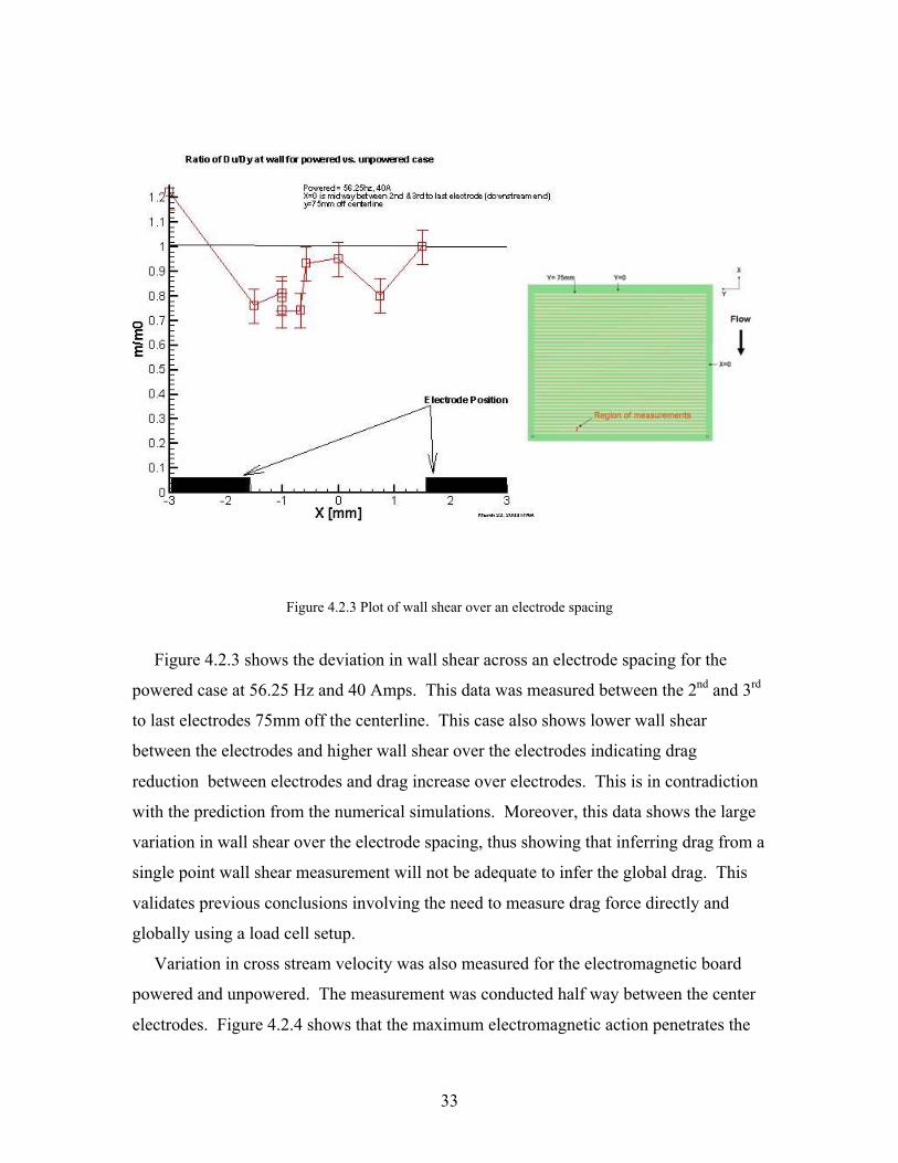
Figure 4.2.3 Plot of wall shear over an electrode spacing

Figure 4.2.3 shows the deviation in wall shear across an electrode spacing for the

powered case at 56.25 Hz and 40 Amps. This data was measured between the 2nd and 3rd

to last electrodes 75mm off the centerline. This case also shows lower wall shear

between the electrodes and higher wall shear over the electrodes indicating drag

reduction between electrodes and drag increase over electrodes. This is in contradiction

with the prediction from the numerical simulations. Moreover, this data shows the large

variation in wall shear over the electrode spacing, thus showing that inferring drag from a

single point wall shear measurement will not be adequate to infer the global drag. This

validates previous conclusions involving the need to measure drag force directly and

globally using a load cell setup.

Variation in cross stream velocity was also measured for the electromagnetic board

powered and unpowered. The measurement was conducted half way between the center

electrodes. Figure 4.2.4 shows that the maximum electromagnetic action penetrates the

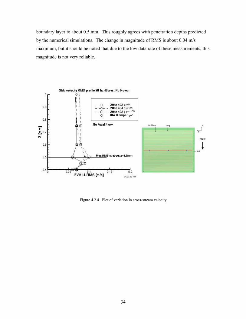
34

boundary layer to about 0.5 mm. This roughly agrees with penetration depths predicted

by the numerical simulations. The change in magnitude of RMS is about 0.04 m/s

maximum, but it should be noted that due to the low data rate of these measurements, this

magnitude is not very reliable.

Figure 4.2.4 Plot of variation in cross-stream velocity

35

4.2.2 Comparisons to prior work

Measurements of wall shear as a function of current amplitude were performed

between the 2nd and 3rd to last electrodes and 75mm off the center of the electrode board.

The figure below compares the data of Jaskolski 2002 [2] to measurements conducted in

March 2003. The data was collected at the same location over the electrode board for

both cases at 1.5 m/s and at frequencies of T+ = 100. The data shows similar trends for

both data though the magnitude of the maximum wall shear variation is lower for the

2003 data. Instead of a magnitude of about 36% in change in du/dy for a current

amplitude of 40 amps measured by Jaskolski [2], the recent measured magnitude for

change in du/dy was about 28%. This change could be due to the high sensitivity to axial

position on the wall shear.

Figure 4.2.5 Wall shear comparison: Present vs. Jaskolski at 1.5 m/s

36

4.3 Force Measurements

4.3.1 Background

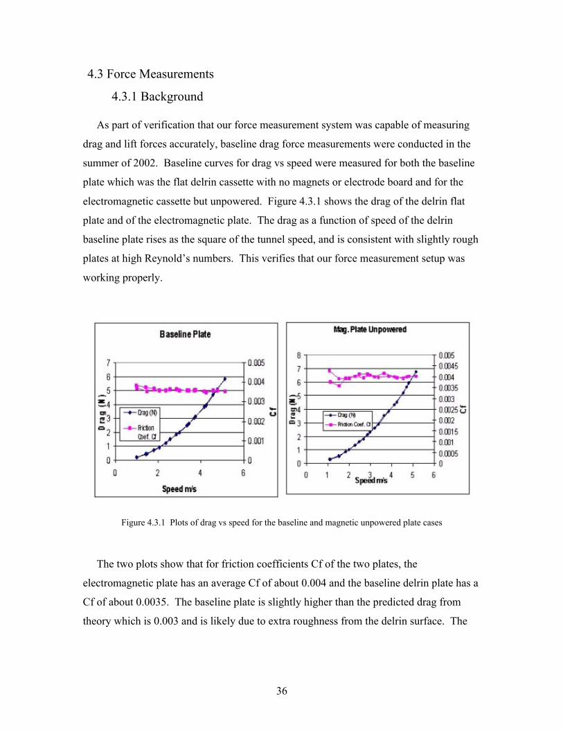
As part of verification that our force measurement system was capable of measuring

drag and lift forces accurately, baseline drag force measurements were conducted in the

summer of 2002. Baseline curves for drag vs speed were measured for both the baseline

plate which was the flat delrin cassette with no magnets or electrode board and for the

electromagnetic cassette but unpowered. Figure 4.3.1 shows the drag of the delrin flat

plate and of the electromagnetic plate. The drag as a function of speed of the delrin

baseline plate rises as the square of the tunnel speed, and is consistent with slightly rough

plates at high Reynold’s numbers. This verifies that our force measurement setup was

working properly.

Figure 4.3.1 Plots of drag vs speed for the baseline and magnetic unpowered plate cases

The two plots show that for friction coefficients Cf of the two plates, the

electromagnetic plate has an average Cf of about 0.004 and the baseline delrin plate has a

Cf of about 0.0035. The baseline plate is slightly higher than the predicted drag from

theory which is 0.003 and is likely due to extra roughness from the delrin surface. The

37

increase in the drag of the electromagnetic plate is probably due to the extra roughness of

the electrodes of the electrode board protruding from the surface.

38

4.3.2 Drag Force Measurements

The process of measuring drag forces in an attempt to verify global drag reduction as a

result of Lorentz force activation was carried out experimentally in March of 2003.

Other attempts had been made in January of 2003 but because of driver electronics and

data acquisition problems, no reliable drag force measurements were conducted. In the

March 2003 force measurement experiment, data acquisition and driver electronics issues

were taken care of and reliable drag measurements were made.

Time [S]

Dra

g[N

]

100 200 300 400 5000

0.25

0.5

0.75

1

1.25

1.5

1.75

2U= 2.25 m/s, Current = 40 Amps , Frequency = 100 Hz

Drag vs Time

3*sigma = 3.317%

Figure 4.3.2 Plot of drag vs time an operating point of U=2.25 m/s, Current = 40 A, Frequency = 100Hz

From this experimental work, figure 4.3.2 shows the repeatability of the drag

measurement at one point. The operating point for this data is at a tunnel speed U

39

equal to 2.25 m/s, a current of 40 Amps, and a driving frequency of 100Hz. This data has

a 3 sigma variation of 3.317% which was used as the error bound for subsequent drag

measurements. In this calculated error bound, the contributions are likely to be from the

resolution of the data acquisition system and from small fluctuations in tunnel speed

which is controlled manually. When controlling tunnel speed, the LDV laser system is

used to measure the flow speed in the free stream. The person running the experiment

will periodically check the flow speed acquired by the LDV system and adjust the tunnel

speed accordingly. After the tunnel impeller has been running for about a half hour, the

resolution of tunnel speed control is 0.01 m/s, which is remarkably good.

Frequency [Hz]

Dra

gD

/Do

50 100 1500

0.25

0.5

0.75

1

1.25

1.5

1.75

2D/Do Vs FrequencyU = 1.5 m/s, Current = 0 Amps

Figure 4.3.3 Plot of drag D/Do vs frequency

Drag measurements were also conducted with the tunnel speed at 1.5 m/s and with the

electromagnetic board unpowered (0 Amps) but at different frequencies. We expect there

to be almost no variation in this case since the output amperage on the power supply

40

with it turned on was set to zero for each of these data points. Figure 4.3.3 shows the

actual data of drag D/Do as a function of frequency when the board was unpowered.

D/Do is the dimensionless value of drag and is calculated by dividing drag measurements

at various powered points by the average value of drag for the unpowered sweep. The

data shows little variation in drag as a function of frequency given the error due to drift in

zeros.

Frequency [Hz]

Cu

rre

nt

[A]

50 100 150

10

20

30

40

Drag D/Do1.033661.026941.020221.01351.006781.000070.9933490.9866310.9799140.9731960.9664780.959760.9530430.9463250.939607

Drag D/Do U= 1.5 m/s

Figure 4.3.4 Countour of drag D/Do vs frequency and current

Drag force measurements were also conducted for various frequencies and amplitudes

of current. Sweeps at different frequencies where the current varied from 0 to 40 amps in

increments of 5 amps were performed. The frequencies of these sweeps were performed

from 0 to 180 Hz and were incremented by 10Hz. Since load cell zero positions shift, the

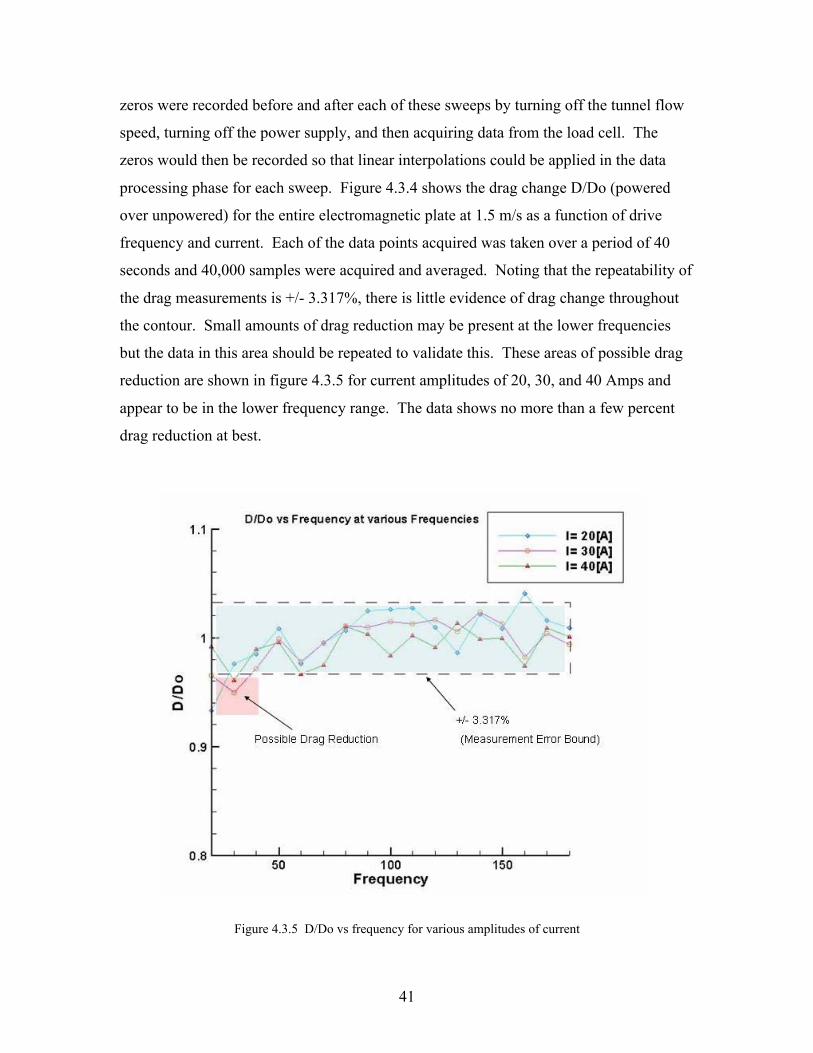
41

zeros were recorded before and after each of these sweeps by turning off the tunnel flow

speed, turning off the power supply, and then acquiring data from the load cell. The

zeros would then be recorded so that linear interpolations could be applied in the data

processing phase for each sweep. Figure 4.3.4 shows the drag change D/Do (powered

over unpowered) for the entire electromagnetic plate at 1.5 m/s as a function of drive

frequency and current. Each of the data points acquired was taken over a period of 40

seconds and 40,000 samples were acquired and averaged. Noting that the repeatability of

the drag measurements is +/- 3.317%, there is little evidence of drag change throughout

the contour. Small amounts of drag reduction may be present at the lower frequencies

but the data in this area should be repeated to validate this. These areas of possible drag

reduction are shown in figure 4.3.5 for current amplitudes of 20, 30, and 40 Amps and

appear to be in the lower frequency range. The data shows no more than a few percent

drag reduction at best.

Figure 4.3.5 D/Do vs frequency for various amplitudes of current

42

Tunnel Speed [m/s]

Dra

g[N

]

0 0.5 1 1.5 2 2.50

0.1

0.2

0.3

0.4

0.5

0.6

0.7

0.8

0.9

1

1.1

1.2

1.3

1.4

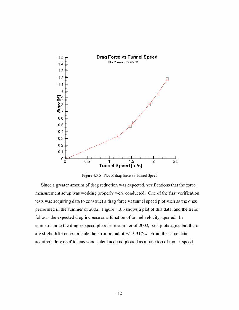
1.5 Drag Force vs Tunnel SpeedNo Power 3-20-03

Figure 4.3.6 Plot of drag force vs Tunnel Speed

Since a greater amount of drag reduction was expected, verifications that the force

measurement setup was working properly were conducted. One of the first verification

tests was acquiring data to construct a drag force vs tunnel speed plot such as the ones

performed in the summer of 2002. Figure 4.3.6 shows a plot of this data, and the trend

follows the expected drag increase as a function of tunnel velocity squared. In

comparison to the drag vs speed plots from summer of 2002, both plots agree but there

are slight differences outside the error bound of +/- 3.317%. From the same data

acquired, drag coefficients were calculated and plotted as a function of tunnel speed.

43

Figure 4.3.7 Plot of Drag Coefficient vs Tunnel Speed for electromagnetic plate

Figure 4.3.7 shows the drag coefficient for the electromagnetic plate as a function of

speed. Note the variation in Cf at 1.5 m/s is about 5% of the total drag. The variation in

drag at lower speeds is due to the decreasing resolution of the drag measurement, since

drag force goes as the square of the velocity. When the data was acquired, the tunnel

speed was varied up to 4m/s and then back down again to a lower speed, hence there is

more than one data point for Cf at some tunnel speeds. Notice there are slight differences

in the drag coefficient for 2002 and 2003 and is likely due to the small bolt in the center

of the electrode board used in the 2003 measurements to keep the board from bowing.

This data verified that the small percentage of global drag reduction was not due to any

problems in the measurement setup. We then proceeded to performing a force time trace

analysis to determine if the electromagnetic forcing had any effect in the fluid.

44

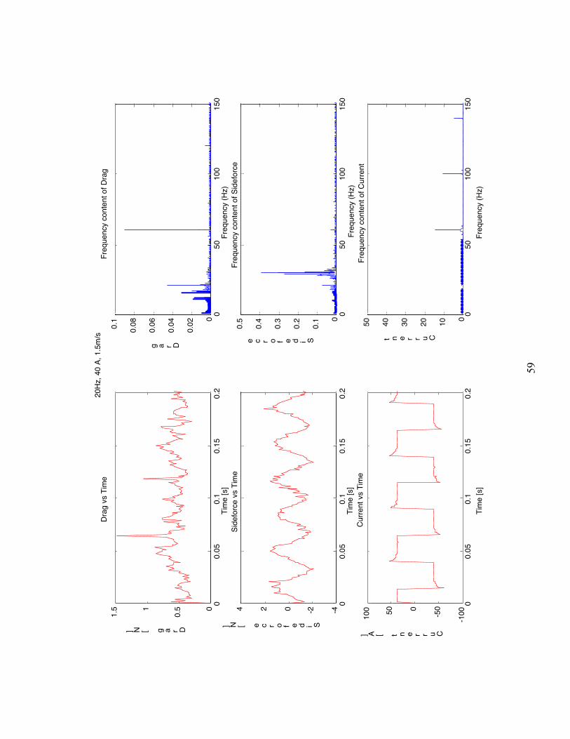
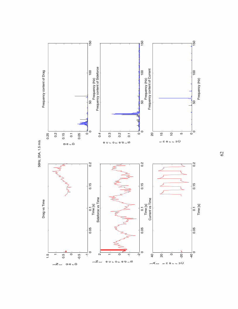
4.3.3 Force time trace data

Force time trace data was taken for a variety of operating points at different

frequencies, amplitudes of current, and tunnel speeds. At some of the operating points,

the effects due to electromagnetic activation were certainly visible. Figure 4.3.7 shows

the time trace and subsequent spectrum of the drag and side forces as well as the current.

In this case, the free-stream tunnel velocity is 0m/s and the board is driven at 100 Hz, and

the drag shows little effect due to electromagnetic forcing. There is some 60 Hz noise

getting into the drag signal. The side force spectrum shows significant content at 100Hz

indicating that electromagnetic force is being input into the fluid. The content at lower

frequencies in both drag and side force are due to resonances in the dynamometer and is

not indicative of any electromagnetic related effects.

Figure 4.3.7 Time trace data and spectra for drag, lift and current

For drag, the plots show that the dynamometer resonance is at about 15 Hz, and for

side force, 28 Hz. In other plots of frequency spectra for side force, for currents of 40

45

amps and frequencies of 100 Hz, but different tunnel speeds greater than zero, the

frequency content almost disappears at 100 Hz. This may be due to a mechanical

interference at flow speeds greater than 1 m/s, where forcing from the fluid on the

floating cassette is masking the electromagnetic forcing effects. It is not ideal for the

frequencies of the responses from electromagnetic forcing to be greater than the

dynamometer resonances for drag and lift. For the case of 3 m/s, the magnitude of the

side force at 100Hz drops to about 0.075 N from the 0.15 N at the 0 m/s case. These

plots can be found in the appendix section. Plots which show the response at no power

were performed on the electromagnetic cassette with the power supply turned off. The

time traces of current for the no power condition at different flow speeds show some

signal getting in, but this is likely due to signal noise or occasionally induced currents

which have magnitudes of less than an amp.

The 28 Hz resonance is present even in the time traces with no power, thus validating

that this resonance is not related to electromagnetic forcing. The data shows that the

frequency of side force is always a multiple of 28Hz, for instance at 100 Hz, 20 Amps,

and 1.5 m/s, there are side force responses at 28Hz and at 56Hz. The frequency

spectrum plots for side force have shown that Lorentz forcing is indeed having an effect

in the fluid at 0 m/s, however for the greater than 0 m/s flow speeds, more research is

needed to determine the cause and effects of the mechanical interference, and whether or

not it is associated with such a low global drag reduction measured in the force

measurement experiment.

46

5.0 Conclusions

Experimental work in the fall and spring of 2002-2003 has shown that Lorentz force

activation does indeed affect the fluid on a local scale. From LDV measurements which

were first acquired by Jaskolski in the spring of 2002, and later validated in the spring of

2003, we can infer that the local drag reduction primarily in between electrodes on the

electrode board was indeed on the order of 30%, a drag reduction amount predicted by

numerical simulations. However, the results from the direct force measurements for drag

with a dynamometer and load cell setup have shown that drag change for a variety of

frequencies and amplitudes of currents have only been on the order of a few percent

taking into consideration that the measurement repeatability was on the order of 3.3%.

This is far less reduction than expected for global drag and the results force us to consider

some of the issues that may have been a factor. Some of these are listed as follows:

• Conductivity: The conductivity of the water in the experimental work was half

of sea water. Since force is proportional to current, a direct impact on force is not

expected, but conductivity may effect ionization, hydrogen formation, iode

heating, and other electrochemical effects. These are expected to be minor effects.

• Magnetic Flux: The magnetic flux at the surface of the electrode board is much

less, on the order of 0.15 Tesla. Decreasing the electrode board thickness would

increase the amount of flux present at the surface of the electrode board exposed

to the flow of water.

• Center bolt in electrode board: This bolt produces locally unwanted drag and

turbulence but is needed to keep the board flat and from bowing at the center. A

better, less intrusive method to hold the board center down would be some type of

adhesive applied to the bottom surface.

• Dynamometer resonance: An unsteady force measurement system whose

resonances are much higher than the drive signal is desirable. Currently, the

resonance response is large compared to the measured forces. The dynamometer

resonances may also cause mechanical interferences with the electromagnetic

forcing.

47

• Base plate turbulence stimulation: Current plate setup has no trips to stimulate

turbulence, thus the transition point could be moving significantly. Installing trips

on this setup would allow more control over turbulence location.

• Base plate flexing at higher speeds: The delrin base plate is not secured at the

leading edge. Some flexing may have occurred. A stiffer plate made of aluminum

with fastening hardware for the leading edge would eliminate any flexing.

• Salt vs sodium nitrite: Electrochemical and ionization differences between salt

and sodium nitrite are expected to cause minor if not negligible effects.

• Square wave improvement: The square wave setup produces less drag

reduction as predicted by numerical simulations.

Another issue that needs to be investigated is whether local drag reduction in between

the electrodes, and drag increase over the electrodes leads to a net drag change of zero for

the entire electrode board. Consultation with Professor Karniadakis to discuss these

issues will be made before any future work is performed on electromagnetic boundary

layer control.

The numerical simulations show that greater drag reduction is present with a traveling

wave Lorentz force, as opposed to a Lorentz force that travels back and forth in the

crosswise flow direction. This would also require more complicated electronic driver

circuitry to create a current wave that travels along the entire electrode board. Hydro

Technologies is currently developing new driver electronics for an experiment with

General Atomics Corp which will be conducted in the water tunnel of the Marine

Hydrodynamics Laboratory in June of 2003. The design of the hardware for this

experiment is currently in progress and involves designing a base plate made of

aluminum, as well as a magnetic filled cassette also made of aluminum that is twice as

long but with the same width as the delrin cassette used in the force measurements in

March of 2003. Flexing of the base plate will be eliminated since the aluminum plate

will be much stiffer and new mounting hardware for setup in the water tunnel is currently

being designed. The electrode board will also have twice the length and will be much

thinner and will allow for a traveling wave that can travel twice the distance. The

48

magnetic flux at the surface of the electrode board is expected to be higher since the

thickness of the new electrode board will be reduced significantly.

Our goals at the Marine Hydrodynamic Laboratory, after having conducted the

traveling wave Lorentz force experiment in June are reliable measurements of drag

reduction as well as a better understanding of why experimental work showed local drag

reduction over the electrode board as predicted by numerical simulations, but global drag

reduction much less than expected. We also hope to identify the possible mechanical

interferences in the dynamometer setup and repeat force time traces once the issues have

been resolved. In the experimental quest for observing a much greater global drag

reduction from Lorentz force activation, we hope to find results that will contribute to

drag reduction efforts that have been carried out for several years in the hydrodynamics

field.

49

References

[1]. Y. Du, V. Symeonidis and G.E. Karniadakis, “Drag reduction in wall-bounded turbulence via a transverse traveling wave”, J. Fluid Mech., Vol. 457, pp.1-34.

[2]. Jaskolski, Corey, “Experimental Implementation of Lorentz Force Actuators for Hydrodynamic Drag”, (Master’s Thesis, Massachusetts Institute of Technology,

May 2002).

[3] UNESCO International Equation of State (IES 80) as described in Fofonoff, JGR, Vol 90 No. C2, pp 3332-3342, March 20, 1985.

50

6.0 Appendix

6.1 Force Time Trace Series

51

Case 1: 0 m/s

00.

050.

10.

150.

2-0

.4

-0.20

0.2

0.4

Tim

e [s

]

Drag [N]

Drag

vs

Tim

e

050

100

150

0

0.02

0.04

0.06

0.080.1

Freq

uenc

y co

nten

t of D

rag

Freq

uenc

y (H

z)

Drag

00.

050.

10.

150.

2-3-2-1012

Tim

e [s

]

Sideforce [N]Si

defo

rce

vs T

ime

050

100

150

0

0.1

0.2

0.3

0.4

0.5

Freq

uenc

y co

nten

t of S

idef

orce

Freq

uenc

y (H

z)

Sideforce

00.

050.

10.

150.

2-1

00-50050100

Tim

e [s

]

Current [A]Cu

rrent

vs

Tim

e

050

100

150

0204060Fr

eque

ncy

cont

ent o

f Cur

rent

Freq

uenc

y (H

z)

Current

28Hz

, 40A

, 0 m

/s

53

00.

050.

10.

150.

2-1

-0.50

0.51

Tim

e [s

]

Drag [N]

Drag

vs

Tim

e

050

100

150

0

0.050.

1

0.150.

2

0.25

Freq

uenc

y co

nten

t of D

rag

Freq

uenc

y (H

z)

Drag

00.

050.

10.

150.

2-2-1012

Tim

e [s

]

Sideforce [N]Si

defo

rce

vs T

ime

050

100

150

0

0.050.

1

0.150.

2Fr

eque

ncy

cont

ent o

f Sid

efor

ce

Freq

uenc

y (H

z)

Sideforce

00.

050.

10.

150.

2-1

00-50050100

Tim

e [s

]

Current [A]Cu

rrent

vs

Tim

e

050

100

150

0204060Fr

eque

ncy

cont

ent o

f Cur

rent

Freq

uenc

y (H

z)

Current

56Hz

, 40A

, 0 m

/s

54

00.

050.

10.

150.

2-3-2-1012

Tim

e [s

]

Drag [N]

Drag

vs

Tim

e

050

100

150

0

0.02

0.04

0.06

0.080.1

Freq

uenc

y co

nten

t of D

rag

Freq

uenc

y (H

z)

Drag

00.

050.

10.

150.

2-2-1012

Tim

e [s

]

Sideforce [N]Si

defo

rce

vs T

ime

050

100

150

0

0.050.1

Freq

uenc

y co

nten

t of S

idef

orce

Freq

uenc

y (H

z)

Sideforce

00.

050.

10.

150.

2-1

00-50050100

Tim

e [s

]

Current [A]Cu

rrent

vs

Tim

e

050

100

150

01020304050Fr

eque

ncy

cont

ent o

f Cur

rent

Freq

uenc

y (H

z)

Current

100H

z, 4

0A, 0

m/s

55

00.

050.

10.

150.

2-0

.4

-0.20

0.2

0.4

0.6

Tim

e [s

]

Drag [N]

Drag

vs

Tim

e

050

100

150

0

0.02

0.04

0.06

0.080.

1Fr

eque

ncy

cont

ent o

f Dra

g

Freq

uenc

y (H

z)

Drag

00.

050.

10.

150.

2-2-1012

Tim

e [s

]

Sideforce [N]Si

defo

rce

vs T

ime

050

100

150

0

0.050.

1

0.150.

2Fr

eque

ncy

cont

ent o

f Sid

efor

ce

Freq

uenc

y (H

z)

Sideforce

00.

050.

10.

150.

2-4-2024

Tim

e [s

]

Current [A]Cu

rrent

vs

Tim

e

050

100

150

0

0.1

0.2

0.3

0.4

0.5

Freq

uenc

y co

nten

t of C

urre

nt

Freq

uenc

y (H

z)

Current

No P

ower

zer

o m

/s

Case 2: 1.5 m/s

00.

050.

10.

150.

20

0.51

1.5

Tim

e [s

]

Drag [N]

Drag

vs

Tim

e

050

100

150

0

0.050.1

0.150.2

0.25

Freq

uenc

y co

nten

t of D

rag

Freq

uenc

y (H

z)

Drag

00.

050.

10.

150.

2-2-1012

Tim

e [s

]

Sideforce [N]Si

defo

rce

vs T

ime

050

100

150

0

0.1

0.2

0.3

0.4

Freq

uenc

y co

nten

t of S

idef

orce

Freq

uenc

y (H

z)

Sideforce

00.

050.

10.

150.

2-1

0-50510

Tim

e [s

]

Current [A]Cu

rrent

vs

Tim

e

050

100

150

0

0.1

0.2

0.3

0.4

0.5

Freq

uenc

y co

nten

t of C

urre

nt

Freq

uenc

y (H

z)

Current

20hz

, 1A,

1.5

m/s

58

00.

050.

10.

150.

2-0

.50

0.51

Tim

e [s

]

Drag [N]

Drag

vs

Tim

e

050

100

150

0

0.050.1

0.150.2

0.25

Freq

uenc

y co

nten

t of D

rag

Freq

uenc

y (H

z)

Drag

00.

050.

10.

150.

2-4-2024

Tim

e [s

]

Sideforce [N]Si

defo

rce

vs T

ime

050

100

150

0

0.050.1

0.150.2

0.25

Freq

uenc

y co

nten

t of S

idef

orce

Freq

uenc

y (H

z)

Sideforce

00.

050.

10.

150.

2-4

0

-2002040

Tim

e [s

]

Current [A]Cu

rrent

vs

Tim

e

050

100

150

0510152025Fr

eque

ncy

cont

ent o

f Cur

rent

Freq

uenc

y (H

z)

Current

20Hz

, 20A

, 1.5

m/s

59

00.

050.

10.

150.

20

0.51

1.5

Tim

e [s

]

Drag [N]

Drag

vs

Tim

e

050

100

150

0

0.02

0.04

0.06

0.080.1

Freq

uenc

y co

nten

t of D

rag

Freq

uenc

y (H

z)

Drag

00.

050.

10.

150.

2-4-2024

Tim

e [s

]

Sideforce [N]Si

defo

rce

vs T

ime

050

100

150

0

0.1

0.2

0.3

0.4

0.5

Freq

uenc

y co

nten

t of S

idef

orce

Freq

uenc

y (H

z)

Sideforce

00.

050.

10.

150.

2-1

00-50050100

Tim

e [s

]

Current [A]Cu

rrent

vs

Tim

e

050

100

150

01020304050Fr

eque

ncy

cont

ent o

f Cur

rent

Freq

uenc

y (H

z)

Current

20Hz

, 40

A, 1

.5m

/s

60

00.

050.

10.

150.

2-1

-0.50

0.51

1.5

Tim

e [s

]

Drag [N]

Drag

vs

Tim

e

050

100

150

0

0.050.1

0.150.2

0.25

Freq

uenc

y co

nten

t of D

rag

Freq

uenc

y (H

z)

Drag

00.

050.

10.

150.

2-3-2-1012

Tim

e [s

]

Sideforce [N]

Side

forc

e vs

Tim

e

050

100

150

0

0.1

0.2

0.3

0.4

0.5

Freq

uenc

y co

nten

t of S

idef

orce

Freq

uenc

y (H

z)

Sideforce

00.

050.

10.

150.

2-1

00-50050100

Tim

e [s

]

Current [A]Cu

rrent

vs

Tim

e

050

100

150

01020304050Fr

eque

ncy

cont

ent o

f Cur

rent

Freq

uenc

y (H

z)

Current

28Hz

, 40A

, 1.5

m/s

61

00.

050.

10.

150.

20

0.2

0.4

0.6

0.81

Tim

e [s

]

Drag [N]

Drag

vs

Tim

e

050

100

150

0

0.050.

1

0.150.

2

0.25

Freq

uenc

y co

nten

t of D

rag

Freq

uenc

y (H

z)

Drag

00.

050.

10.

150.

2-2-1012

Tim

e [s

]

Sideforce [N]Si

defo

rce

vs T

ime

050

100

150

0

0.1

0.2

0.3

0.4

Freq

uenc

y co

nten

t of S

idef

orce

Freq

uenc

y (H

z)

Sideforce

00.

050.

10.

150.

2-1

0-50510

Tim

e [s

]

Current [A]Cu

rrent

vs

Tim

e

050

100

150

0

0.1

0.2

0.3

0.4

0.5

Freq

uenc

y co

nten

t of C

urre

nt

Freq

uenc

y (H

z)

Current

56Hz

, 1A,

1.5

m/s

62

00.

050.

10.

150.

2-1

-0.50

0.51

1.5

Tim

e [s

]

Drag [N]

Drag

vs

Tim

e

050

100

150

0

0.050.

1

0.150.

2

0.25

Freq

uenc

y co

nten

t of D

rag

Freq

uenc

y (H

z)

Drag

00.

050.

10.

150.

2-2-1012

Tim

e [s

]

Sideforce [N]Si

defo

rce

vs T

ime

050

100

150

0

0.1

0.2

0.3

0.4

Freq

uenc

y co

nten

t of S

idef

orce

Freq

uenc

y (H

z)

Sideforce

00.

050.

10.

150.

2-4

0

-2002040

Tim

e [s

]

Current [A]Cu

rrent

vs

Tim

e

050

100

150

05101520Fr

eque

ncy

cont

ent o

f Cur

rent

Freq

uenc

y (H

z)

Current

56Hz

, 20A

, 1.5

m/s

63

00.

050.

10.

150.

2-0

.50

0.51

1.5

Tim

e [s

]

Drag [N]

Drag

vs

Tim

e

050

100

150

0

0.050.

1

0.150.

2

0.25

Freq

uenc

y co

nten

t of D

rag

Freq

uenc

y (H

z)

Drag

00.

050.

10.

150.

2-2-1012

Tim

e [s

]

Sideforce [N]Si

defo

rce

vs T

ime

050

100

150

0

0.1

0.2

0.3

0.4

Freq

uenc

y co

nten

t of S

idef

orce

Freq

uenc

y (H

z)

Sideforce

00.

050.

10.

150.

2-1

00-50050100

Tim

e [s

]

Current [A]Cu

rrent

vs

Tim

e

050

100

150

010203040Fr

eque

ncy

cont

ent o

f Cur

rent

Freq

uenc

y (H

z)

Current

56Hz

, 40A

, 1.5

m/s

64

00.

050.

10.

150.

20

0.2

0.4

0.6

0.81

Tim

e [s

]

Drag [N]

Drag

vs

Tim

e

050

100

150

0

0.050.1

0.150.2

0.25

Freq

uenc

y co

nten

t of D

rag

Freq

uenc

y (H

z)

Drag

00.

050.

10.

150.

2-2-1012

Tim

e [s

]

Sideforce [N]Si

defo

rce

vs T

ime

050

100

150

0

0.1

0.2

0.3

0.4

Freq

uenc

y co

nten

t of S

idef

orce

Freq

uenc

y (H

z)

Sideforce

00.

050.

10.

150.

2-2-10123

Tim

e [s

]

Current [A]Cu

rrent

vs

Tim

e

050

100

150

0

0.2

0.4

0.6

0.8

Freq

uenc

y co

nten

t of C

urre

nt

Freq

uenc

y (H

z)

Current

100H

z, 1

A, 1

.5m

/s

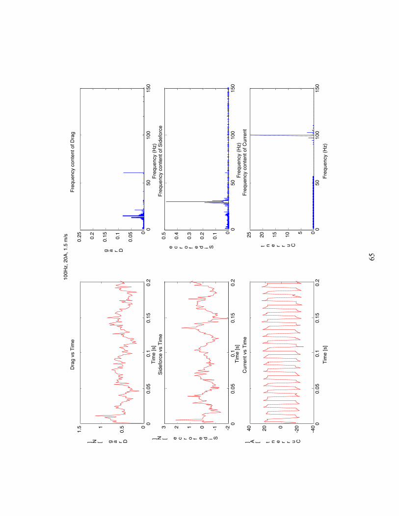
65

00.

050.

10.

150.

20

0.51

1.5

Tim

e [s

]

Drag [N]

Drag

vs

Tim

e

050

100

150

0

0.050.1

0.150.2

0.25

Freq

uenc

y co

nten

t of D

rag

Freq

uenc

y (H

z)

Drag

00.

050.

10.

150.

2-2-10123

Tim

e [s

]

Sideforce [N]Si

defo

rce

vs T

ime

050

100

150

0

0.1

0.2

0.3

0.4

0.5

Freq

uenc

y co

nten

t of S

idef

orce

Freq

uenc

y (H

z)

Sideforce

00.

050.

10.

150.

2-4

0

-2002040

Tim

e [s

]

Current [A]Cu

rrent

vs

Tim

e

050

100

150

0510152025Fr

eque

ncy

cont

ent o

f Cur

rent

Freq

uenc

y (H

z)

Current

100H

z, 2

0A, 1

.5 m

/s

66

00.

050.

10.

150.

20

0.2

0.4

0.6

0.81

Tim

e [s

]

Drag [N]

Drag

vs

Tim

e

050

100

150

0

0.050.

1

0.150.

2

0.25

Freq

uenc

y co

nten

t of D

rag

Freq

uenc

y (H

z)

Drag

00.

050.

10.

150.

2-2-1012

Tim

e [s

]

Sideforce [N]Si

defo

rce

vs T

ime

050

100

150

0

0.1

0.2

0.3

0.4

0.5

Freq

uenc

y co

nten

t of S

idef

orce

Freq

uenc

y (H

z)

Sideforce

00.

050.

10.

150.

2-4-2024

Tim

e [s

]

Current [A]Cu

rrent

vs

Tim

e

050

100

150

0

0.1

0.2

0.3

0.4

0.5

Freq

uenc

y co

nten

t of C

urre

nt

Freq

uenc

y (H

z)

Current

No P

ower

, 1.5

m/s

Case 3: 3.0 m/s

00.

050.

10.

150.

201234

Tim

e [s

]

Drag [N]

Drag

vs

Tim

e

050

100

150

0

0.1

0.2

0.3

0.4

0.5

Freq

uenc

y co

nten

t of D

rag

Freq

uenc

y (H

z)

Drag

00.

050.

10.

150.

2-6-4-2024

Tim

e [s

]

Sideforce [N]Si

defo

rce

vs T

ime

050

100

150

0

0.51

1.5

Freq

uenc

y co

nten

t of S

idef

orce

Freq

uenc

y (H

z)

Sideforce

00.

050.

10.

150.

2-4

0

-2002040

Tim

e [s

]

Current [A]Cu

rrent

vs

Tim

e

050

100

150

0510152025Fr

eque

ncy

cont

ent o

f Cur

rent

Freq

uenc

y (H

z)

Current

20Hz

, 20A

, 3m

/s

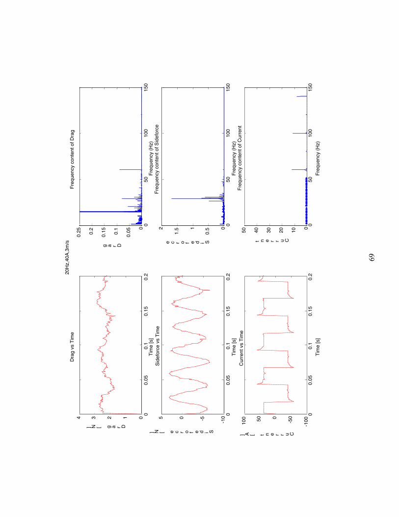
69

00.

050.

10.

150.

201234

Tim

e [s

]

Drag [N]

Drag

vs

Tim

e

050

100

150

0

0.050.1

0.150.2

0.25

Freq

uenc

y co

nten

t of D

rag

Freq

uenc

y (H

z)

Drag

00.

050.

10.

150.

2-1

0-505

Tim

e [s

]

Sideforce [N]Si

defo

rce

vs T

ime

050

100

150

0

0.51

1.52

Freq

uenc

y co

nten

t of S

idef

orce

Freq

uenc

y (H

z)

Sideforce

00.

050.

10.

150.

2-1

00-50050100

Tim

e [s

]

Current [A]Cu

rrent

vs

Tim

e

050

100

150

01020304050Fr

eque

ncy

cont

ent o

f Cur

rent

Freq

uenc

y (H

z)

Current

20Hz

,40A

,3m

/s

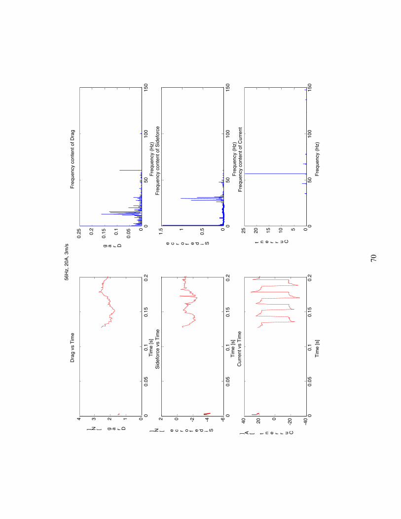
70

00.

050.

10.

150.

201234

Tim

e [s

]

Drag [N]

Drag

vs

Tim

e

050

100

150

0

0.050.

1

0.150.

2

0.25

Freq

uenc

y co

nten

t of D

rag

Freq

uenc

y (H

z)

Drag

00.

050.

10.

150.

2-6-4-202

Tim

e [s

]

Sideforce [N]Si

defo

rce

vs T

ime

050

100

150

0

0.51

1.5

Freq

uenc

y co

nten

t of S

idef

orce

Freq

uenc

y (H

z)

Sideforce

00.

050.

10.

150.

2-4

0

-2002040

Tim

e [s

]

Current [A]Cu

rrent

vs

Tim

e

050

100

150

0510152025Fr

eque

ncy

cont

ent o

f Cur

rent

Freq

uenc

y (H

z)

Current

56Hz

, 20A

, 3m

/s

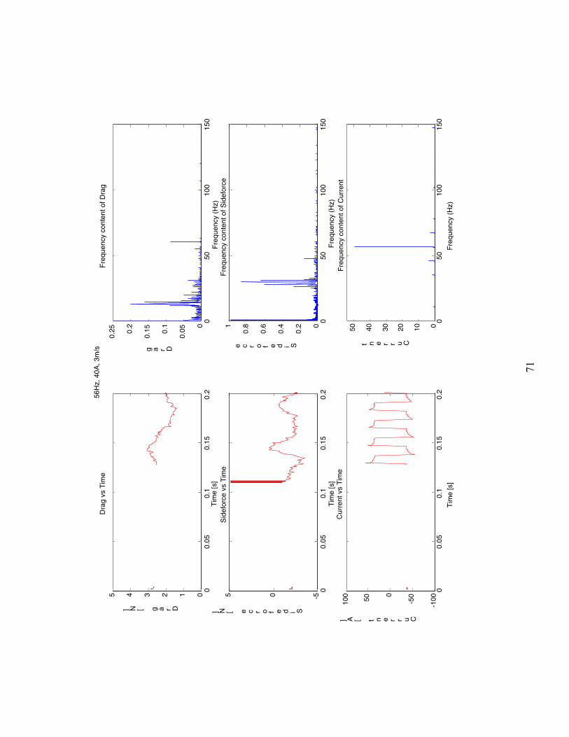
71

00.

050.

10.

150.

2012345

Tim

e [s

]

Drag [N]

Drag

vs

Tim

e

050

100

150

0

0.050.

1

0.150.

2

0.25

Freq

uenc

y co

nten

t of D

rag

Freq

uenc

y (H

z)

Drag

00.

050.

10.

150.

2-505

Tim

e [s

]

Sideforce [N]Si

defo

rce

vs T

ime

050

100

150

0

0.2

0.4

0.6

0.81

Freq

uenc

y co

nten

t of S

idef

orce

Freq

uenc

y (H

z)

Sideforce

00.

050.

10.

150.

2-1

00-50050100

Tim

e [s

]

Current [A]Cu

rrent

vs

Tim

e

050

100

150

01020304050Fr

eque

ncy

cont

ent o

f Cur

rent

Freq

uenc

y (H

z)

Current

56Hz

, 40A

, 3m

/s

72

00.

050.

10.

150.

201234

Tim

e [s

]

Drag [N]

Drag

vs

Tim

e

050

100

150

0

0.2

0.4

Freq

uenc

y co

nten

t of D

rag

Freq

uenc

y (H

z)

Drag

00.

050.

10.

150.

2

-6-4-2024

Tim

e [s

]

Sideforce [N]Si

defo

rce

vs T

ime

050

100

150

0

0.51

1.5

Freq

uenc

y co

nten

t of S

idef

orce

Freq

uenc

y (H

z)

Sideforce

00.

050.

10.

150.

2-5

0050

Tim

e [s

]

Current [A]Cu

rrent

vs

Tim

e

050

100

150

0510152025Fr

eque

ncy

cont

ent o

f Cur

rent

Freq

uenc

y (H

z)

Current

100H

z, 2

0A, 3

m/s

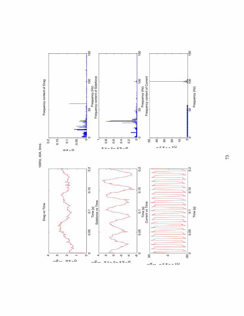
73

00.

050.

10.

150.

201234

Tim

e [s

]

Drag [N]

Drag

vs

Tim

e

050

100

150

0

0.050.1

0.150.2

Freq

uenc

y co

nten

t of D

rag

Freq

uenc

y (H

z)

Drag

00.

050.

10.

150.

2-6-4-2024

Tim

e [s

]

Sideforce [N]Si

defo

rce

vs T

ime

050

100

150

0

0.2

0.4

0.6

0.81

Freq

uenc

y co

nten

t of S

idef

orce

Freq

uenc

y (H

z)

Sideforce

00.

050.

10.

150.

2-5

0050

Tim

e [s

]

Current [A]Cu

rrent

vs

Tim

e

050

100

150

01020304050Fr

eque

ncy

cont

ent o

f Cur

rent

Freq

uenc

y (H

z)

Current

100H

z, 4

0A, 3

m/s

74

00.

050.

10.

150.

201234

Tim

e [s

]

Drag [N]

Drag

vs

Tim

e

050

100

150

0

0.1

0.2

0.3

Freq

uenc

y co

nten

t of D

rag

Freq

uenc

y (H

z)

Drag

00.

050.

10.

150.

2-4-202

Tim

e [s

]

Sideforce [N]Si

defo

rce

vs T

ime

050

100

150

0

0.51

1.5

Freq

uenc

y co

nten

t of S

idef

orce

Freq

uenc

y (H

z)

Sideforce

00.

050.

10.

150.

2-4-2024

Tim

e [s

]

Current [A]Cu

rrent

vs

Tim

e

050

100

150

0

0.1

0.2

0.3

0.4

0.5

Freq

uenc

y co

nten

t of C

urre

nt

Freq

uenc

y (H

z)

Current

No P

ower

, 3 m

/s

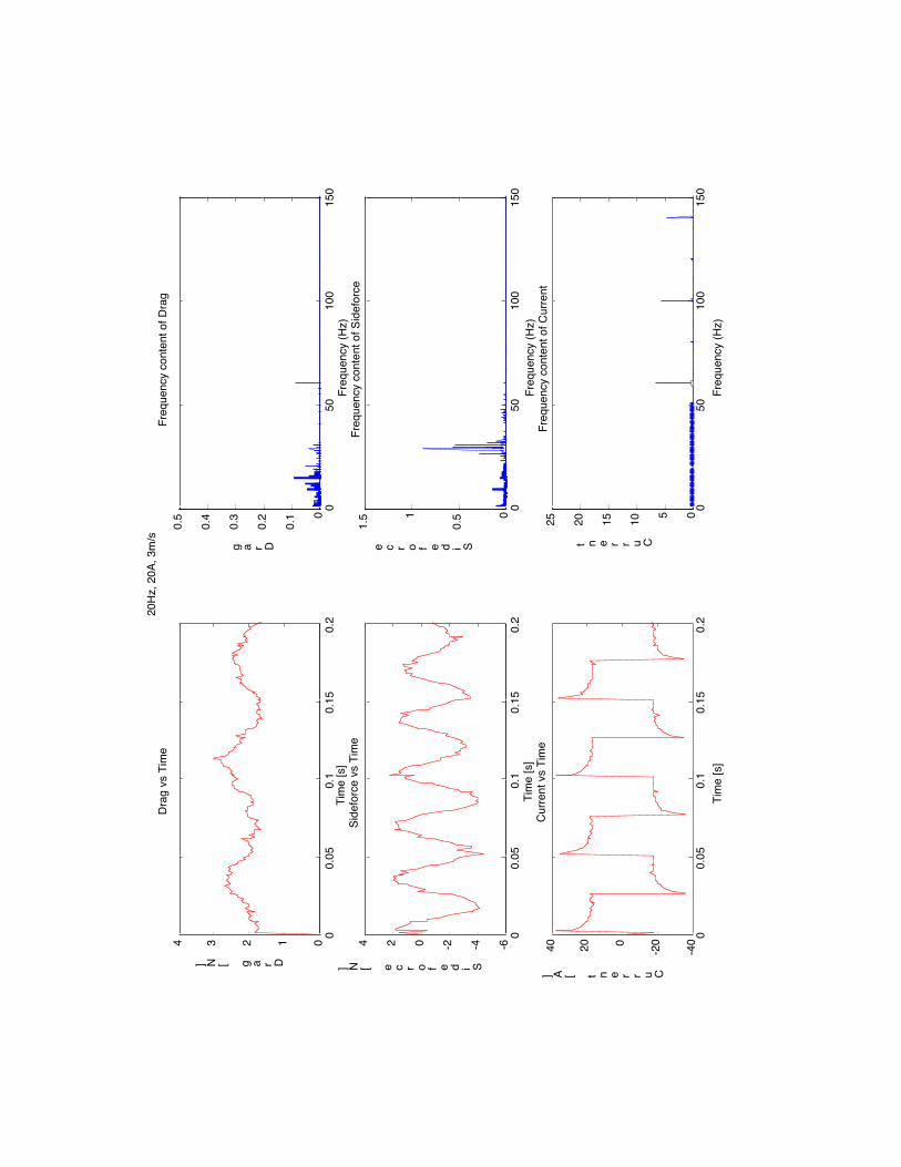
00.

050.

10.

150.

201234

Tim

e [s

]

Drag [N]

Drag

vs

Tim

e

050

100

150

0

0.1

0.2

0.3

0.4

0.5

Freq

uenc

y co

nten

t of D

rag

Freq

uenc

y (H

z)

Drag

00.

050.

10.

150.

2-6-4-2024

Tim

e [s

]

Sideforce [N]Si

defo

rce

vs T

ime

050

100

150

0

0.51

1.5

Freq

uenc

y co

nten

t of S

idef

orce

Freq

uenc

y (H

z)

Sideforce

00.

050.

10.

150.

2-4

0

-2002040

Tim

e [s

]

Current [A]Cu

rrent

vs

Tim

e

050

100

150

0510152025Fr

eque

ncy

cont

ent o

f Cur

rent

Freq

uenc

y (H

z)

Current

20Hz

, 20A

, 3m

/s

69

00.

050.

10.

150.

201234

Tim

e [s

]

Drag [N]

Drag

vs

Tim

e

050

100

150

0

0.050.1

0.150.2

0.25

Freq

uenc

y co

nten

t of D

rag

Freq

uenc

y (H

z)

Drag

00.

050.

10.

150.

2-1

0-505

Tim

e [s

]

Sideforce [N]Si

defo

rce

vs T

ime

050

100

150

0

0.51

1.52

Freq

uenc

y co

nten

t of S

idef

orce

Freq

uenc

y (H

z)

Sideforce

00.

050.

10.

150.

2-1

00-50050100

Tim

e [s

]

Current [A]Cu

rrent

vs

Tim

e

050

100

150

01020304050Fr

eque

ncy

cont

ent o

f Cur

rent

Freq

uenc

y (H

z)

Current

20Hz

,40A

,3m

/s

70

00.

050.

10.

150.

201234

Tim

e [s

]

Drag [N]

Drag

vs

Tim

e

050

100

150

0

0.050.

1

0.150.

2

0.25

Freq

uenc

y co

nten

t of D

rag

Freq

uenc

y (H

z)

Drag

00.

050.

10.

150.

2-6-4-202

Tim

e [s

]

Sideforce [N]Si

defo

rce

vs T

ime

050

100

150

0

0.51

1.5

Freq

uenc

y co

nten

t of S

idef

orce

Freq

uenc

y (H

z)

Sideforce

00.

050.

10.

150.

2-4

0

-2002040

Tim

e [s

]

Current [A]Cu

rrent

vs

Tim

e

050

100

150

0510152025Fr

eque

ncy

cont

ent o

f Cur

rent

Freq

uenc

y (H

z)

Current

56Hz

, 20A

, 3m

/s

71

00.

050.

10.

150.

2012345

Tim

e [s

]

Drag [N]

Drag

vs

Tim

e

050

100

150

0

0.050.

1

0.150.

2

0.25

Freq

uenc

y co

nten

t of D

rag

Freq

uenc

y (H

z)

Drag

00.

050.

10.

150.

2-505

Tim

e [s

]

Sideforce [N]Si

defo

rce

vs T

ime

050

100

150

0

0.2

0.4

0.6

0.81

Freq

uenc

y co

nten

t of S

idef

orce

Freq

uenc

y (H

z)

Sideforce

00.

050.

10.

150.

2-1

00-50050100

Tim

e [s

]

Current [A]Cu

rrent

vs

Tim

e

050

100

150

01020304050Fr

eque

ncy

cont

ent o

f Cur

rent

Freq

uenc

y (H

z)

Current

56Hz

, 40A

, 3m

/s

72

00.

050.

10.

150.

201234

Tim

e [s

]

Drag [N]

Drag

vs

Tim

e

050

100

150

0

0.2

0.4

Freq

uenc

y co

nten

t of D

rag

Freq

uenc

y (H

z)

Drag

00.

050.

10.

150.

2

-6-4-2024

Tim

e [s

]

Sideforce [N]Si

defo

rce

vs T

ime

050

100

150

0

0.51

1.5

Freq

uenc

y co

nten

t of S

idef

orce

Freq

uenc

y (H

z)

Sideforce

00.

050.

10.

150.

2-5

0050

Tim

e [s

]

Current [A]Cu

rrent

vs

Tim

e

050

100

150

0510152025Fr

eque

ncy

cont

ent o

f Cur

rent

Freq

uenc

y (H

z)

Current

100H

z, 2

0A, 3

m/s

73

00.

050.

10.

150.

201234

Tim

e [s

]

Drag [N]

Drag

vs

Tim

e

050

100

150

0

0.050.1

0.150.2

Freq

uenc

y co

nten

t of D

rag

Freq

uenc

y (H

z)

Drag

00.

050.

10.

150.

2-6-4-2024

Tim

e [s

]

Sideforce [N]Si

defo

rce

vs T

ime

050

100

150

0

0.2

0.4

0.6

0.81

Freq

uenc

y co

nten

t of S

idef

orce

Freq

uenc

y (H

z)

Sideforce

00.

050.

10.

150.

2-5

0050

Tim

e [s

]

Current [A]Cu

rrent

vs

Tim

e

050

100

150

01020304050Fr

eque

ncy

cont

ent o

f Cur

rent

Freq

uenc

y (H

z)

Current

100H

z, 4

0A, 3

m/s

74

00.

050.

10.

150.

201234

Tim

e [s

]

Drag [N]

Drag

vs

Tim

e

050

100

150

0

0.1

0.2

0.3

Freq

uenc

y co

nten

t of D

rag

Freq

uenc

y (H

z)

Drag

00.

050.

10.

150.

2-4-202

Tim

e [s

]

Sideforce [N]Si

defo

rce

vs T

ime

050

100

150

0

0.51

1.5

Freq

uenc

y co

nten

t of S

idef

orce

Freq

uenc

y (H

z)

Sideforce

00.

050.

10.

150.

2-4-2024

Tim

e [s

]

Current [A]Cu

rrent

vs

Tim

e

050

100

150

0

0.1

0.2

0.3

0.4

0.5

Freq

uenc

y co

nten

t of C

urre

nt

Freq

uenc

y (H

z)

Current

No P

ower

, 3 m

/s

Case 1: 0 m/s

00.

20.

40.

60.

81

-0.4

-0.20

0.2

0.4

0.6

Tim

e [s

]

Drag [N]

Drag

vs

Tim

e

050

100

150

10-5

100

Freq

uenc

y co

nten

t of D

rag

Freq

uenc

y (H

z)

Drag

00.

20.

40.

60.

81

-4-2024

Tim

e [s

]

Sideforce [N]Si

defo

rce

vs T

ime

050

100

150

10-5

100

Freq

uenc

y co

nten

t of S

idef

orce

Freq

uenc

y (H

z)

Sideforce

00.

20.

40.

60.

81

-100-5

0050100

Tim

e [s

]

Current [A]Cu

rrent

vs

Tim

e

050

100

150

10-4

10-2

100

102

Freq

uenc

y co

nten

t of C

urre

nt

Current

28Hz

, 40A

, 0 m

/s

Freq

uenc

y (H

z)

77

00.

20.

40.

60.

81

-0.50

0.5

Tim

e [s

]

Drag [N]

Drag

vs

Tim

e

2040

6080

100

120

140

10-5

100

Freq

uenc

y co

nten

t of D

rag

Freq

uenc

y (H

z)

Drag

00.

20.

40.

60.

81

-2-1012

Tim

e [s

]

Sideforce [N]Si

defo

rce

vs T

ime

050

100

150

10-5

100

Freq

uenc

y co

nten

t of S

idef

orce

Freq

uenc

y (H

z)

Sideforce

00.

20.

40.

60.

81

-100-50050100

Tim

e [s

]

Current [A]Cu

rrent

vs

Tim

e

050

100

150

10-4

10-2

100

102

Freq

uenc

y co

nten

t of C

urre

nt

Freq

uenc

y (H

z)

Current

56 H

z, 4

0 A,

0m

/s

78

00.

20.

40.

60.

81

-3-2-1012

Tim

e [s

]

Drag [N]

Drag

vs

Tim

e

050

100

150

10-5

100

Freq

uenc

y co

nten

t of D

rag

Freq

uenc

y (H

z)

Drag

00.

20.

40.

60.

81

-4-202

Tim

e [s

]

Sideforce [N]Si

defo

rce

vs T

ime

050

100

150

10-5

100

Freq

uenc

y co

nten

t of S

idef

orce

Freq

uenc

y (H

z)

Sideforce

00.

20.

40.

60.

81

-100-5

0050100

Tim

e [s

]

Current [A]Cu

rrent

vs

Tim

e

050

100

150

10-4

10-2

100

102

Freq

uenc

y co

nten

t of C

urre

nt

Freq

uenc

y (H

z)

Current

100H

z, 4

0A, 0

m/s

79

00.

20.

40.

60.

81

-1

-0.50

0.5

Tim

e [s

]

Drag [N]

Drag

vs

Tim

e

050

100

150

10-6

10-4

10-2

100

Freq

uenc

y co

nten

t of D

rag

Freq

uenc

y (H

z)

Drag

00.

20.

40.

60.

81

-2-1012

Tim

e [s

]

Sideforce [N]Si

defo

rce

vs T

ime

050

100

150

10-5

100

Freq

uenc

y co

nten

t of S

idef

orce

Freq

uenc

y (H

z)

Sideforce

00.

20.

40.

60.

81

-6-4-2024

Tim

e [s

]

Current [A]Cu

rrent

vs

Tim

e

050

100

150

10-5

100

Freq

uenc

y co

nten

t of C

urre

nt

Current

No P

ower

zer

o m

/s

Freq

uenc

y (H

z)

Case 2: 1.5 m/s

00.

20.

40.

60.

81

-0.50

0.51

1.5

Tim

e [s

]

Drag [N]Dr

ag v

s Ti

me

050

100

150

10-1

0

10-5

100

105

Freq

uenc

y co

nten

t of D

rag

Freq

uenc

y (H

z)

Drag

00.

20.

40.

60.

81

-2-1012

Tim

e [s

]

Sideforce [N]Si

defo

rce

vs T

ime

050

100

150

10-5

100

Freq

uenc

y co

nten

t of S

idef

orce

Freq

uenc

y (H

z)

Sideforce

00.

20.

40.

60.

81

-10-50510

Tim

e [s

]

Current [A]Cu

rrent

vs

Tim

e

050

100

150

10-5

100

Freq

uenc

y co

nten

t of C

urre

nt

Current

20hz

, 1A,

1.5

m/s

Freq

uenc

y (H

z)

82

00.

20.

40.

60.

81

-0.50

0.51

Tim

e [s

]

Drag [N]

Drag

vs

Tim

e

050

100

150

10-5

100

105

Freq

uenc

y co

nten

t of D

rag

Freq

uenc

y (H

z)

Drag

00.

20.

40.

60.

81

-4-2024

Tim

e [s

]

Sideforce [N]Si

defo

rce

vs T

ime

050

100

150

10-4

10-2

100

Freq

uenc

y co

nten

t of S

idef

orce

Freq

uenc

y (H

z)

Sideforce

00.

20.

40.

60.

81

-40

-2002040

Tim

e [s

]

Current [A]Cu

rrent

vs

Tim

e

050

100

150

10-4

10-2

100

102

Freq

uenc

y co

nten

t of C

urre

nt

Freq

uenc

y (H

z)

Current

20Hz

, 20A

, 1.5

m/s

83

00.

20.

40.

60.

81

0

0.51

1.5

Tim

e [s

]

Drag [N]

Drag

vs

Tim

e

050

100

150

10-5

100

105

Freq

uenc

y co

nten

t of D

rag

Freq

uenc

y (H

z)

Drag

00.

20.

40.

60.

81

-4-2024

Tim

e [s

]

Sideforce [N]Si

defo

rce

vs T

ime

050

100

150

10-5

100

Freq

uenc

y co

nten

t of S

idef

orce

Freq

uenc

y (H

z)

Sideforce

00.

20.

40.

60.

81

-100-5

0050100

Tim

e [s

]

Current [A]Cu

rrent

vs

Tim

e

050

100

150

10-4

10-2

100

102

Freq

uenc

y co

nten

t of C

urre

nt

Current

20Hz

, 40

A, 1

.5m

/s

Freq

uenc

y (H

z)

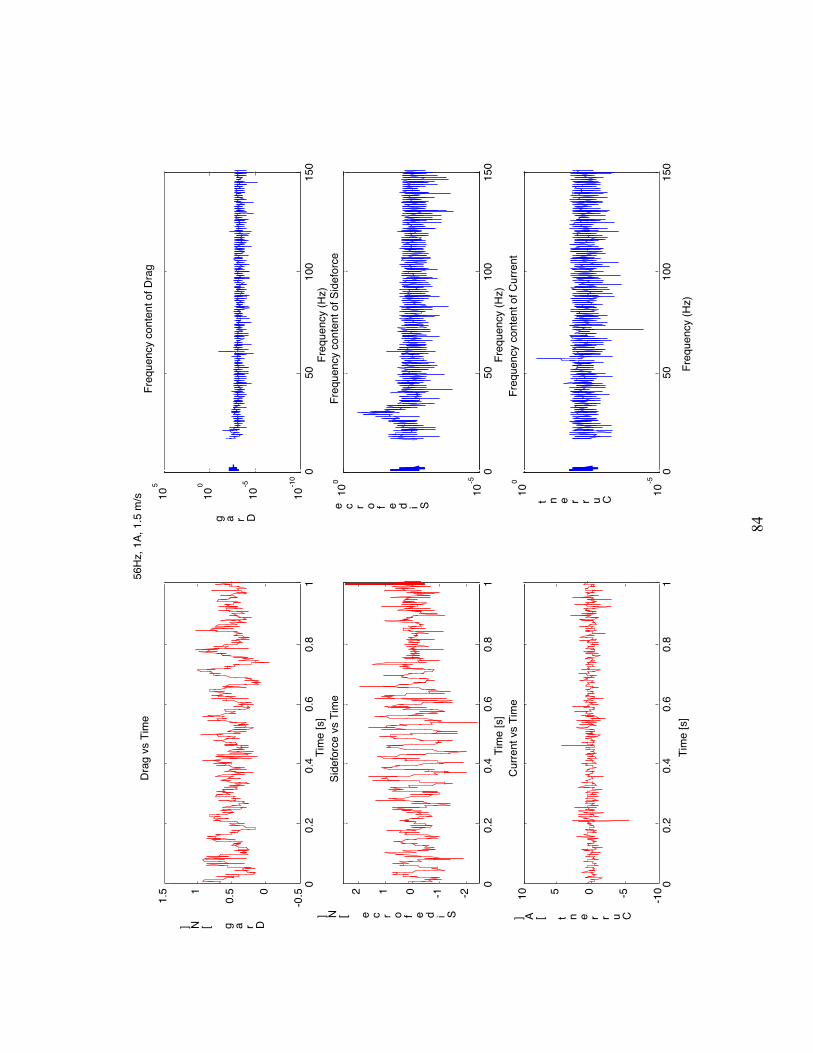
84

00.

20.

40.

60.

81

-0.50

0.51

1.5

Tim

e [s

]

Drag [N]

Drag

vs

Tim

e

050

100

150

10-1

0

10-5

100

105

Freq

uenc

y co

nten

t of D

rag

Freq

uenc

y (H

z)

Drag

00.

20.

40.

60.

81

-2-1012

Tim

e [s

]

Sideforce [N]Si

defo

rce

vs T

ime

050

100

150

10-5

100

Freq

uenc

y co

nten

t of S

idef

orce

Freq

uenc

y (H

z)

Sideforce

00.

20.

40.

60.

81

-10-50510

Tim

e [s

]

Current [A]Cu

rrent

vs

Tim

e

050

100

150

10-5

100

Freq

uenc

y co

nten

t of C

urre

nt

Current

56Hz

, 1A,

1.5

m/s

Freq

uenc

y (H

z)

85

00.

20.

40.

60.

81

-1

-0.50

0.51

1.5

Tim

e [s

]

Drag [N]

Drag

vs

Tim

e

050

100

150

10-1

0

10-5

100

105

Freq

uenc

y co

nten

t of D

rag

Freq

uenc

y (H

z)

Drag

00.

20.

40.

60.

81

-2-1012

Tim

e [s

]

Sideforce [N]Si

defo

rce

vs T

ime

050

100

150

10-5

100

Freq

uenc

y co

nten

t of S

idef

orce

Freq

uenc

y (H

z)

Sideforce

00.

20.

40.

60.

81

-40

-2002040

Tim

e [s

]

Current [A]Cu

rrent

vs

Tim

e

050

100

150

10-4

10-2

100

102

Freq

uenc

y co

nten

t of C

urre

nt

Current

56Hz

, 20A

, 1.5

m/s

Freq

uenc

y (H

z)

86

00.

20.

40.

60.

81

-10123

Tim

e [s

]

Drag [N]

Drag

vs

Tim

e

050

100

150

10-5

100

105

Freq

uenc

y co

nten

t of D

rag

Freq

uenc

y (H

z)

Drag

00.

20.

40.

60.

81

-2-1012

Tim

e [s

]

Sideforce [N]Si

defo

rce

vs T

ime

050

100

150

10-5

100

Freq

uenc

y co

nten

t of S

idef

orce

Freq

uenc

y (H

z)

Sideforce

00.

20.

40.

60.

81

-100-5

0050100

Tim

e [s

]

Current [A]Cu

rrent

vs

Tim

e

050

100

150

10-4

10-2

100

102

Freq

uenc

y co

nten

t of C

urre

nt

Current

56Hz

, 40A

, 1.5

m/s

Freq

uenc

y (H

z)

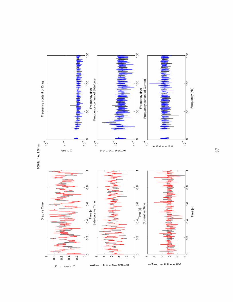
87

00.

20.

40.

60.

81

0

0.2

0.4

0.6

0.81

Tim

e [s

]

Drag [N]

Drag

vs

Tim

e

050

100

150

10-5

100

105

Freq

uenc

y co

nten

t of D

rag

Freq

uenc

y (H

z)

Drag

00.

20.

40.

60.

81

-3-2-1012

Tim

e [s

]

Sideforce [N]Si

defo

rce

vs T

ime

050

100

150

10-4

10-2

100

Freq

uenc

y co

nten

t of S

idef

orce

Freq

uenc

y (H

z)

Sideforce

00.

20.

40.

60.

81

-4-20246

Tim

e [s

]

Current [A]Cu

rrent

vs

Tim

e

050

100

150

10-5

100

Freq

uenc

y co

nten

t of C

urre

nt

Current

100H

z, 1

A, 1

.5m

/s

Freq

uenc

y (H

z)

88

00.

20.

40.

60.

81

-1012

Tim

e [s

]

Drag [N]

Drag

vs

Tim

e

050

100

150

10-1

0

10-5

100

105

Freq

uenc

y co

nten

t of D

rag

Freq

uenc

y (H

z)

Drag

00.

20.

40.

60.

81

-3-2-10123

Tim

e [s

]

Sideforce [N]Si

defo

rce

vs T

ime

050

100

150

10-5

100

Freq

uenc

y co

nten

t of S

idef

orce

Freq

uenc

y (H

z)

Sideforce

00.

20.

40.

60.

81

-4-20246

Tim

e [s

]

Current [A]Cu

rrent

vs

Tim

e

050

100

150

10-4

10-2

100

Freq

uenc

y co

nten

t of C

urre

nt

Current

No P

ower

1.5

m/s

Freq

uenc

y (H

z)

Case 3: 3.0 m/s

00.

20.

40.

60.

81

01234

Tim

e [s

]

Drag [N]

Drag

vs

Tim

e

050

100

150

10-5

100

105

Freq

uenc

y co

nten

t of D

rag

Freq

uenc

y (H

z)

Drag

00.

20.

40.

60.

81

-6-4-2024

Tim

e [s

]

Sideforce [N]Si

defo

rce

vs T

ime

050

100

150

10-4

10-2

100

102

Freq

uenc

y co

nten

t of S

idef

orce

Freq

uenc

y (H

z)

Sideforce

00.

20.

40.

60.

81

-40

-2002040

Tim

e [s

]

Current [A]Cu

rrent

vs

Tim

e

050

100

150

10-4

10-2

100

102

Freq

uenc

y co

nten

t of C

urre

nt

Current

20Hz

, 20A

, 3m

/s

Freq

uenc

y (H

z)

91

00.

20.

40.

60.

81

01234

Tim

e [s

]

Drag [N]

Drag

vs

Tim

e

050

100

150

10-5

100

105

Freq

uenc

y co

nten

t of D

rag

Freq

uenc

y (H

z)

Drag

00.

20.

40.

60.

81

-10-505

Tim

e [s

]

Sideforce [N]Si

defo

rce

vs T

ime

050

100

150

10-4

10-2

100

102

Freq

uenc

y co

nten

t of S

idef

orce

Freq

uenc

y (H

z)

Sideforce

00.

20.

40.

60.

81

-100-5

0050100

Tim

e [s

]

Current [A]Cu

rrent

vs

Tim

e

050

100

150

10-4

10-2

100

102

Freq

uenc

y co

nten

t of C

urre

nt

Freq

uenc

y (H

z)

Current

20Hz

,40A

,3m

/s

92

00.

20.

40.

60.

81

01234

Tim

e [s

]

Drag [N]

Drag

vs

Tim

e

050

100

150

10-5

100

105

Freq

uenc

y co

nten

t of D

rag

Freq

uenc

y (H

z)

Drag

00.

20.

40.

60.

81

-10-50510

Tim

e [s

]

Sideforce [N]Si

defo

rce

vs T

ime

050

100

150

10-5

100

105

Freq

uenc

y co

nten

t of S

idef

orce

Freq

uenc

y (H

z)

Sideforce

00.

20.

40.

60.

81

-40

-2002040

Tim

e [s

]

Current [A]Cu

rrent

vs

Tim

e

050

100

150

10-4

10-2

100

102

Freq

uenc

y co

nten

t of C

urre

nt

Current

56Hz

, 20A

, 3m

/s

Freq

uenc

y (H

z)

Freq

uenc

y (H

z)

93

00.

20.

40.

60.

81

012345

Tim

e [s

]

Drag [N]

Drag

vs

Tim

e

050

100

150

10-5

100

105

Freq

uenc

y co

nten

t of D

rag

Freq

uenc

y (H

z)

Drag

00.

20.

40.

60.

81

-6-4-20246

Tim

e [s

]

Sideforce [N]Si

defo

rce

vs T

ime

050

100

150

10-4

10-2

100

102

Freq

uenc

y co

nten

t of S

idef

orce

Freq

uenc

y (H

z)

Sideforce

00.

20.

40.

60.

81

-100-5

0050100

Tim

e [s

]

Current [A]Cu

rrent

vs

Tim

e

050

100

150

10-2

100

Freq

uenc

y co

nten

t of C

urre

nt

Freq

uenc

y (H

z)

Current

56Hz

, 40A

, 3m

/s

94

00.

20.

40.

60.

81

01234

Tim

e [s

]

Drag [N]

Drag

vs

Tim

e

050

100

150

10-5

100

105

Freq

uenc

y co

nten

t of D

rag

Freq

uenc

y (H

z)

Drag

00.

20.

40.

60.

81

-6-4-2024

Tim

e [s

]

Sideforce [N]Si

defo

rce

vs T

ime

050

100

150

10-5

100

105

Freq

uenc

y co

nten

t of S

idef

orce

Freq

uenc

y (H

z)

Sideforce

00.

20.

40.

60.

81

-50050

Tim

e [s

]

Current [A]Cu

rrent

vs

Tim

e

050

100

150

10-4

10-2

100

102

Freq

uenc

y co

nten

t of C

urre

nt

Current

100H

z, 2

0A, 3

m/s

Freq

uenc

y (H

z)

95

00.

20.

40.

60.

81

01234

Tim

e [s

]

Drag [N]

Drag

vs

Tim

e

050

100

150

10-5

100

105

Freq

uenc

y co

nten

t of D

rag

Freq

uenc

y (H

z)

Drag

00.

20.

40.

60.

81

-6-4-2024

Tim

e [s

]

Sideforce [N]Si

defo

rce

vs T

ime

050

100

150

10-4

10-2

100

102

Freq

uenc

y co

nten

t of S

idef

orce

Freq

uenc

y (H

z)

Sideforce

00.

20.

40.

60.

81

-100-5

0050100

Tim

e [s

]

Current [A]Cu

rrent

vs

Tim

e

050

100

150

10-4

10-2

100

102

Freq

uenc

y co

nten

t of C

urre

nt

Current

100H

z, 4

0A, 3

m/s

Freq

uenc

y (H

z)

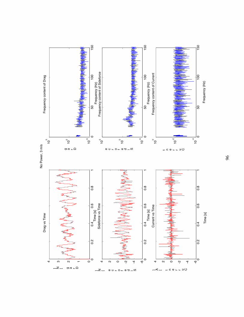
96

00.

20.

40.

60.

81

01234

Tim

e [s

]

Drag [N]

Drag

vs

Tim

e

050

100

150

10-5

100

105

Freq

uenc

y co

nten

t of D

rag

Freq

uenc

y (H

z)

Drag

00.

20.

40.

60.

81

-6-4-2024

Tim

e [s

]

Sideforce [N]Si

defo

rce

vs T

ime

050

100

150

10-5

100

105

Freq

uenc

y co

nten

t of S

idef

orce

Freq

uenc

y (H

z)

Sideforce

00.

20.

40.

60.

81

-6-4-2024

Tim

e [s

]

Current [A]Cu

rrent

vs

Tim

e

050

100

150

10-4

10-2

100

Freq

uenc

y co

nten

t of C

urre

nt

Current

No P

ower

, 3 m

/s

Freq

uenc

y (H

z)

6.2 Electronics Schematics

98

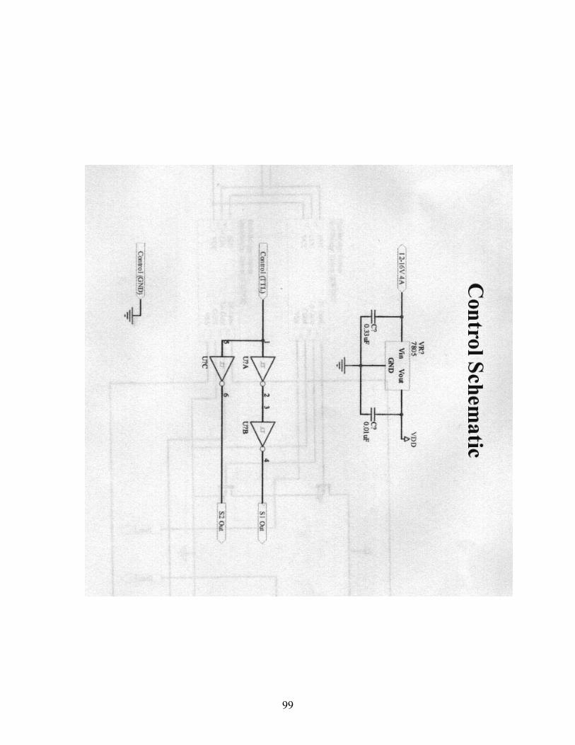
99

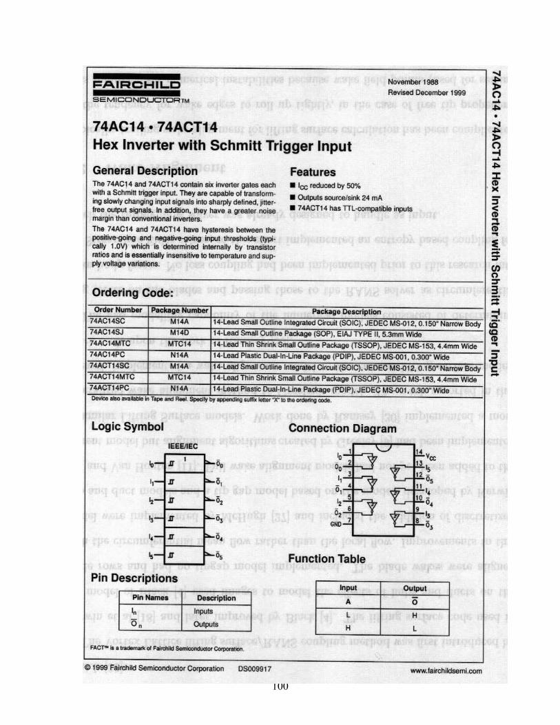
100

101