Applied Energy 112 (2013) 300–312

Contents lists available at SciVerse ScienceDirect

Applied Energy

journal homepage: www.elsevier .com/ locate/apenergy

Electrical, thermal and structural performance of a cooled PV module:Transient analysis using a multiphysics model

0306-2619/$ - see front matter � 2013 Elsevier Ltd. All rights reserved.http://dx.doi.org/10.1016/j.apenergy.2013.06.030

⇑ Corresponding author.E-mail addresses: afmarif@kfupm.edu.sa, afmarif1@gmail.com (A.F.M. Arif).

M.U. Siddiqui, A.F.M. Arif ⇑Department of Mechanical Engineering, King Fahd University of Petroleum and Minerals, Dhahran 31261, Saudi Arabia

h i g h l i g h t s

�Multiphysics model for electrical, thermal and structural performance prediction.� Structural performance of PV modules is important under thermal cycling and cooling.� Methodology for coupling thermal and electrical model of PV modules.� Simulations done for four different full days representing different timings of a year.� Cooling effectiveness is most strongly dependent on incident solar radiation.

a r t i c l e i n f o

Article history:Received 22 November 2012Received in revised form 11 June 2013Accepted 15 June 2013Available online 9 July 2013

Keywords:Photovoltaic moduleMultiphysics modelThermal modelElectrical modelStructural modelThermal stress

a b s t r a c t

The main performance metric of any PV device is its electrical power output. But the ability to predict itsthermal and structural response under different environmental conditions are also important in order toestimate its overall performance and for useful life prediction and reliability analysis. In the current work,the development of a multiphysics model is presented which is capable of estimating the three dimen-sional thermal and structural performance as well as the electrical performance of a PV module undergiven meteorological conditions. The model is also capable of including the effect of module cooling.The thermal modeling has been carried out in ANSYS CFX CFD environment, the structural modelinghas been done in ANSYS Mechanical FEA code and the electrical modeling has been developed in MATLABenvironment. The electrical model used is an improved seven-parameter electric circuit model which iscapable of better simulating the electrical performance of the module at low irradiance and high temper-ature conditions. A coupling methodology to include the effect of electrical performance of the PV modulein the thermal model inside the CFD environment has also been presented in the paper. Using the devel-oped model, the electrical, thermal and structural performance of a PV module with and without coolinghas been analyzed for four different days representing different environmental conditions at Jeddah,Saudi Arabia.

� 2013 Elsevier Ltd. All rights reserved.

1. Introduction

Photovoltaic technology (PV) provides a direct method to con-vert solar energy into electricity. In recent years, the use of PV sys-tems has increased greatly with many applications of PV devices insystems as small as battery chargers to large scale electricity gen-eration systems and satellite power systems. Commercially avail-able PV modules convert around 13–20% of incident solarradiation into electricity. The remaining solar energy absorbed intothe panel is converted to heat and increases the panel temperature.This increase in temperature causes the development of thermalstresses in the panel and also causes the module efficiency to de-crease [1]. To reduce the panel temperature, cooling of the PV pan-

els is usually done which improves the electrical performance ofthe module and reduces the thermal stresses developing in themodule.

Several types of thermal models have been developed for calcu-lating the temperature of PV cells as a function of solar radiationand the environmental conditions. These include models for PVpanels without cooling [2–4] as well as with cooling [5–10]. ForPV module cooling two different approaches have been adopted.Either custom-made photovoltaic–thermal (PV/T) collectors aredeveloped with the objective of PV module cooling and collectinghot water or air or commercially available PV modules are cooledusing auxiliary thermal collectors attached to the back surface ofthe module.

Thermal modeling of custom-made PV/T collectors is exten-sively reported in literature [5–8]. Tiwari and Sodha [5] developeda one-dimensional analytical model for the Integrated

Nomenclature

a modified diode ideality factoraref modified diode ideality factor at STCAi anisotropy indexApanel area of PV panel (m2)[B] displacement gradient matrixCp specific heat capacity (J/kg K)Cl, Ce1, Ce2 constants for turbulence model[D] material properties matrix (Pa)Eg band-gap energy of PV cell material (eV)Eg,ref band-gap energy of PV cell material at STC (eV){Fth} thermal force vector (N)Ffront/rear-ground geometric factor for front glass or back sheet to

ground radiationFfront/rear-sky geometric factor for front glass or back sheet to sky

radiationGb horizontal beam radiation (W/m2)Gd horizontal diffuse radiation (W/m2)Gref reference condition (STC) incident radiation (W/m2)h heat loss coefficient (W/m2 K)hconv,forced forced convection coefficient (W/m2 K)hconv,free free convection coefficient (W/m2 K)hradiation radiation heat loss coefficient (W/m2 K)I PV panel output current (A)IL light generated current (A)IL,ref light generated current at STC (A)IMP PV panel maximum power current (A)Io diode reverse saturation current (A)Io,ref diode reverse saturation current at STC (A)kcond thermal conductivity (W/m K)k turbulent kinetic energy (m2/s2)K extinction coefficient[K] stiffness matrix (N/m)Ksa,b incidence angle modifier for beam radiationKsa,d incidence angle modifier for diffuse radiationKsa,g incidence angle modifier for ground reflected radiationLglass thickness of front glass layer (m)m irradiance dependence parameter for IL

M air mass modifiern temperature dependence parameter for an surface normalNCS number of PV cell in series in PV panelNu Nusselt’s numberPk production termPr Prandl’s numberq heat conduction (W)Q volumetric heat generation (W/m3)Qvh viscous energy dissipation (W/m3)Rbeam geometric factor for beam radiation

Ra Raleigh’s numberRe Reynolds’s numberRs series resistance (X)Rs,ref series resistance at STC (X)Rsh shunt resistance (X)Rsh.ref shunt resistance at STC (X)S plane-of-array absorbed solar radiation at operating

conditions (W/m2)Sref absorbed solar radiation at STC (W/m2)t time (s)T(x,y,z) temperature field (K)Tamb ambient temperature (K)Tcell PV cells temperature (K)Tcell,ref PV cells temperature at STC (K)Tf,in inlet water temperature (K)Tfront/rear temperature of front or back surface (K)Tsky sky temperature (K)u fluid velocity (m/s){u} displacement vector (m)V PV panel output voltage (V)VMP PV panel maximum power voltage (V)Vf,in inlet water velocity (m/s)Vpv,cell volume of PV cells inside the module (m3)

Greek symbolsa absorptivity of PV cellsb slope of PV panelgpv electrical efficiency of PV panelgpv,ref PV electrical efficiency at reference condition{e} elastic strain vector{eth} thermal strain vector{eT} total strain vectore turbulent dissipation rate (m2/s3)efront.rear emissivity of front glass or back sheeteground emissivity of groundqground reflectivity of groundq density (kg/m3)h incidence angle of solar radiationhr refracted angle of solar radiationre turbulent Prandtl number for erk turbulent Prandtl number for ks transmitivity of top cover(sa) transmitivity–absorptivity productl dynamic viscosity (Pa s)lisc temperature coefficient of short circuit currentlT turbulent viscosity (Pa s)

M.U. Siddiqui, A.F.M. Arif / Applied Energy 112 (2013) 300–312 301

photovoltaic/thermal system (IPVTS) collector of Huang et al. [11]and validated its performance against experimental data. Animprovement to this model was suggested by Sarhaddi et al. [6].They suggested that the accuracy of the model could be improvedby using the equivalent electric circuit model to determine theelectrical performance of the system and by using more detailedexpressions for determining the thermal resistances within thesystem. A similar model was developed by Amori and Taqi Al-Naj-jar [7] who applied their model to predict the performance of a PV/T collector for two different environmental conditions in Iraq. Theyconsidered the temperature variation across the thickness only andused an equivalent electric circuit model for electrical output pre-diction. Amrizal et al. [8] carried out dynamic modeling of a PV/T

collector. They used a very simplified thermal model which calcu-lated the thermal power output and the PV cell temperature andtheir model required experimental data for estimating the modelparameters. For electrical performance prediction, they used anequivalent electric circuit model.

For a commercially available PV module cooled by auxiliarythermal collectors, a relatively smaller amount of work has beenreported. In one work, Teo et al. [9] designed an air cooled PV/Tsystem using a commercially available PV panel and a custommade air collector attached to it. They developed a one-dimen-sional thermal model for their PV/T collector and used it to analyzeits performance. In a previous work done by the authors, theydeveloped a three-dimensional thermal model for commercial PV

Fig. 1. Performance modeling of PV systems [10].

Fig. 2. Equivalent circuit of an actual PV cell [10].

Fig. 3. Modes of energy transfer in a PV panel [10].

Table 1Material properties used in thermal model.

Material Layer Thermalconductivity(W/m K)

Specificheatcapacity(J/kg K)

Density(kg/m3)

Silicon Solar cell 130 677 2330Tempered glass Top cover 2 500 2450Polyester Bottom

cover0.15 1250 1200

Ethyl vinyl acetate Encapsulent 0.311 2090 950Aluminum Heat

exchanger237 903 2702

Table 2Material properties used in the structural model.

Material Layer Modulusofelasticity(GPa)

Poisson’sratio

Coefficient ofthermalexpansion(K�1)

Silicon Solar cell 150 0.17 2.616 � 10�6

Tempered glass Top cover 70 0.22 9 � 10�6

Polyester Bottomcover

4 0.37 60 � 10�6

EVA Encapsulant 7.8 0.3 90 � 10�6

Aluminum 72 0.32 22 � 10�6

302 M.U. Siddiqui, A.F.M. Arif / Applied Energy 112 (2013) 300–312

modules cooled using an auxiliary thermal collector. They used themodel to carry out parametric studies to see the effect of variousenvironmental and operating parameters include the contact resis-tance between the PV module and thermal collector on the electri-cal and thermal performance of the PV module [10].

For modeling the electrical performance of PV modules, variouselectrical models have been developed. These include modelsbased on the analytical knowledge of PV cell behavior, modelsbased on empirical correlations, as well as models which combinethe two approaches. King et al. [3] developed an empirical modelfor simulation of PV systems called the Sandia Labs PV Model. His-hikawa et al. [12] and Marion et al. [13] used current–voltage curve

interpolation for estimating the module electrical performance.Another approach adapted for PV electrical performance predictionwas to represent the PV device by an equivalent electric circuit inwhich five model parameters represent the specific characteristicsof a PV device. The model parameters can be modified for differentinput conditions and the model can then be solved to find the PVelectrical characteristics [14–16]. The inputs to the electrical mod-el are the absorbed solar radiation in the PV cells and the PV cellstemperature. An improvement to the five parameters model, theseven parameters model, was suggested by the authors [17] in

Fig. 4. Coupling methodology for thermal and electrical models.

Fig. 5. Model validation for thermal model without cooling using experimentaldata [10].

Table 3Model validation for thermal model with cooling [10].

Inlet velocity(m/s)

Cell temperature (�C) Outlet fluid temperature (�C)

Currentmodel

Using Sarhaddiet al. [6]

Currentmodel

Using Sarhaddiet al. [6]

0.1 30.6 29.1 25.7 25.60.05 32.5 31.5 26.5 26.10.01 41.1 39.8 30.7 26.3

Fig. 6. Maximum power prediction errors. (Module 1 = AP-110, Module 2 = S-36,Module 3 = KC-40T, Module 4 = MST-43LV, Module 5 = ST-35, Module 6 = PVL-124).

M.U. Siddiqui, A.F.M. Arif / Applied Energy 112 (2013) 300–312 303

which the equations to modify the model parameters were ad-justed to improve the electrical model accuracy at low irradiancesand high temperatures.

As far as structural performance of PV panels is concerned, themain approach used is using finite element methods [18–21]. In aneffort to optimize the design of PV cell interconnects to reducethermal stresses, Eitner et al. [18] developed a structural modelfor a string to PV cells laminate using finite element method. Themodel was exposed to uniform temperature loads from 150 �C to�40 �C and the thermal stresses were calculated in a static time-independent analysis. Gonzalez et al. [19] used an FEA based modelto study the effect of encapsulent and adhesive materials and PVcell size on the thermal stresses developing in the cells and theinterconnects. Meuwissen et al. [20] developed a finite elementmodel for a single PV cell laminate to study the structural responseof adhesive cell interconnects. Using the developed FE model, theystudied the effect of adhesive interconnect on the stresses

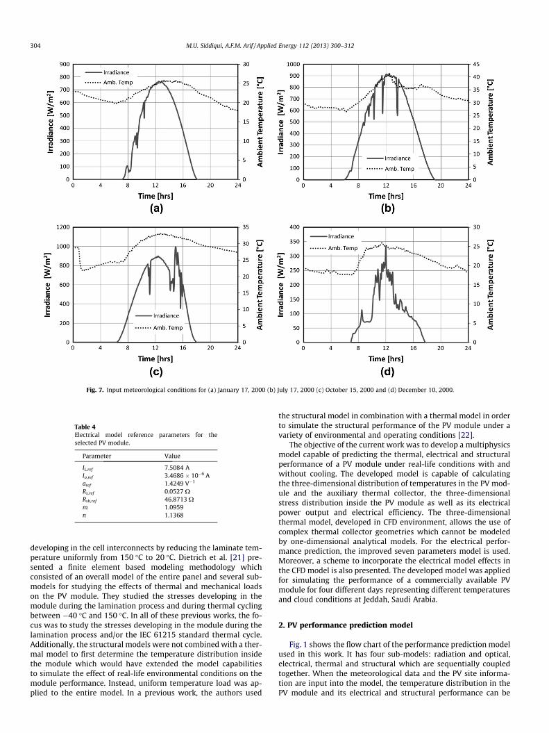
Fig. 7. Input meteorological conditions for (a) January 17, 2000 (b) July 17, 2000 (c) October 15, 2000 and (d) December 10, 2000.

Table 4Electrical model reference parameters for theselected PV module.

Parameter Value

IL,ref 7.5084 AIo,ref 3.4686 � 10�6 Aaref 1.4249 V�1

Rs,ref 0.0527 XRsh,ref 46.8713 Xm 1.0959n 1.1368

304 M.U. Siddiqui, A.F.M. Arif / Applied Energy 112 (2013) 300–312

developing in the cell interconnects by reducing the laminate tem-perature uniformly from 150 �C to 20 �C. Dietrich et al. [21] pre-sented a finite element based modeling methodology whichconsisted of an overall model of the entire panel and several sub-models for studying the effects of thermal and mechanical loadson the PV module. They studied the stresses developing in themodule during the lamination process and during thermal cyclingbetween �40 �C and 150 �C. In all of these previous works, the fo-cus was to study the stresses developing in the module during thelamination process and/or the IEC 61215 standard thermal cycle.Additionally, the structural models were not combined with a ther-mal model to first determine the temperature distribution insidethe module which would have extended the model capabilitiesto simulate the effect of real-life environmental conditions on themodule performance. Instead, uniform temperature load was ap-plied to the entire model. In a previous work, the authors used

the structural model in combination with a thermal model in orderto simulate the structural performance of the PV module under avariety of environmental and operating conditions [22].

The objective of the current work was to develop a multiphysicsmodel capable of predicting the thermal, electrical and structuralperformance of a PV module under real-life conditions with andwithout cooling. The developed model is capable of calculatingthe three-dimensional distribution of temperatures in the PV mod-ule and the auxiliary thermal collector, the three-dimensionalstress distribution inside the PV module as well as its electricalpower output and electrical efficiency. The three-dimensionalthermal model, developed in CFD environment, allows the use ofcomplex thermal collector geometries which cannot be modeledby one-dimensional analytical models. For the electrical perfor-mance prediction, the improved seven parameters model is used.Moreover, a scheme to incorporate the electrical model effects inthe CFD model is also presented. The developed model was appliedfor simulating the performance of a commercially available PVmodule for four different days representing different temperaturesand cloud conditions at Jeddah, Saudi Arabia.

2. PV performance prediction model

Fig. 1 shows the flow chart of the performance prediction modelused in this work. It has four sub-models: radiation and optical,electrical, thermal and structural which are sequentially coupledtogether. When the meteorological data and the PV site informa-tion are input into the model, the temperature distribution in thePV module and its electrical and structural performance can be

M.U. Siddiqui, A.F.M. Arif / Applied Energy 112 (2013) 300–312 305

predicted. The details of the sub-models have been discussed in de-tail in the following sections.

2.1. Electrical model

The electrical model used in the present work is a newly devel-oped 7 parameters model [23] in which a PV device is representedby an equivalent electric circuit [24] of Fig. 2 and the current–volt-age relationship for the PV devices is governed by the followingequation:

I ¼ IL � Io � expV þ I � Rs

a

� �� 1

� �� V þ I � Rs

Rshð1Þ

To use the model, the parameters IL, Io, a, Rs and Rsh are firstdetermined at a reference condition and then translated to theoperating condition using the translation Eqs. (2)–(6). The param-eters m and n are determined using two additional maximumpower values at a higher temperature and a lower irradiance.

a ¼ aref ðTcell=Tcell;ref Þn ð2ÞIL ¼ ðS=Sref ÞmðIL;ref þ liscðTcell � Tcell;ref ÞÞ ð3Þ

Io ¼ Io;ref ðTcell=Tcell;ref Þ3eNCS:Tcell;ref

arefðEg;ref =Tcell;ref�Eg=TcellÞ

� �ð4Þ

Rsh ¼Sref

SRsh;ref ð5Þ

Rs ¼ Rs;ref ð6Þ

2.2. Thermal model

A thermal model to calculate the three-dimensional tempera-ture distribution in PV panels was developed and validated by

Fig. 8. Temporal variation of cell temperature in PV panel for (a) January 17,

the authors in [10]. The model is capable of calculating PV paneltemperature distribution with and without considering PV panelcooling. A PV panel consists of several solid domains for whichthe energy equation need to be solved. In case of cooling, the en-ergy equations for the heat exchanger body and working fluidand the continuity and momentum equations for the working fluidalso need to be solved. Eqs. (7) and (8) are the heat transfer equa-tions for solid and fluid domains respectively [25].

qiCp;i@Tiðx; y; zÞ

@t¼ r � ðqiÞ þ Q i i ¼ 1;2; . . . ;n ð7Þ

qCp@T@tþ qCpu � rTðx; y; zÞ ¼ r � ðqÞ þ Qvh ð8Þ

where

q ¼ kcondrT ð9Þ

and q is the density, Cp is the specific heat capacity, T(x,y,z) is thetemperature, t is the time, kcond is the thermal conductivity, q isthe heat transferred by conduction, Q is the internal heat genera-tion, u is the fluid velocity and Qvh is the viscous dissipation.

The momentum and continuity equations governing the fluidflow inside the heat exchanger are given by Eqs. (10) and (11) [26].

q@u@tþ qðu � rÞu ¼ r � �pI þ ðlþ lTÞðruþruTÞ � 2

3qkI

� �ð10Þ

qr � u ¼ 0 ð11Þ

where p is the pressure, l is the viscosity, lT is the turbulent viscos-ity and k is the turbulent kinetic energy [26].

For a PV panel, the various modes of energy transfer in the PVpanel are shown in Fig. 3. The panel gains energy by absorbingincoming solar radiation while energy is lost from it by convectionand radiation to the environment, by energy transfer to the

2000 (b) July 17, 2000 (c) October 15, 2000 and (d) December 10, 2000.

306 M.U. Siddiqui, A.F.M. Arif / Applied Energy 112 (2013) 300–312

working fluid in the heat exchanger and in the form of electricalenergy delivered to the electrical load. In case of PV panel withoutcooling, the energy transfer to the heat exchanger through the PVpanel back surface is replaced by convection and radiation lossesto the environment.

The absorbed solar radiation was calculated using HDKR model[27,28] and applied to the heat transfer equation of the PV celllayer as an internal heat generation, Q, which was calculated usingthe following equation:

Q ¼ð1� gpvÞ � S� Apanel

Vpvcellð12Þ

where gpv is the electrical efficiency of the PV panel, Apanel is thefront area of the PV panel and the Vpv cell is the volume of the PVcells in the panel.

The PV panel loses heat from its top and bottom surfacesthrough convection and radiation. The equivalent heat loss coeffi-cient for the PV panel is given by the following equation:

h ¼ hconv;forced þ hconv;free þ hradiation ð13Þ

where h is the equivalent heat loss coefficient. Eq. (14) by Sparrowet al. [29], Eq. (15) by Lloyd and Moran [30] and Eq. (16) by Duffieand Beckman [28] can be used to calculate hconv,forced, hconv,free andhradiation iteratively for each time step.

Nu ¼ 0:86Re1=2Pr1=3 ð14Þ

Nu ¼ 0:76Ra1=4 for 104 < Ra < 107

0:15Ra1=3 for 107 < Ra < 3� 1010

(ð15Þ

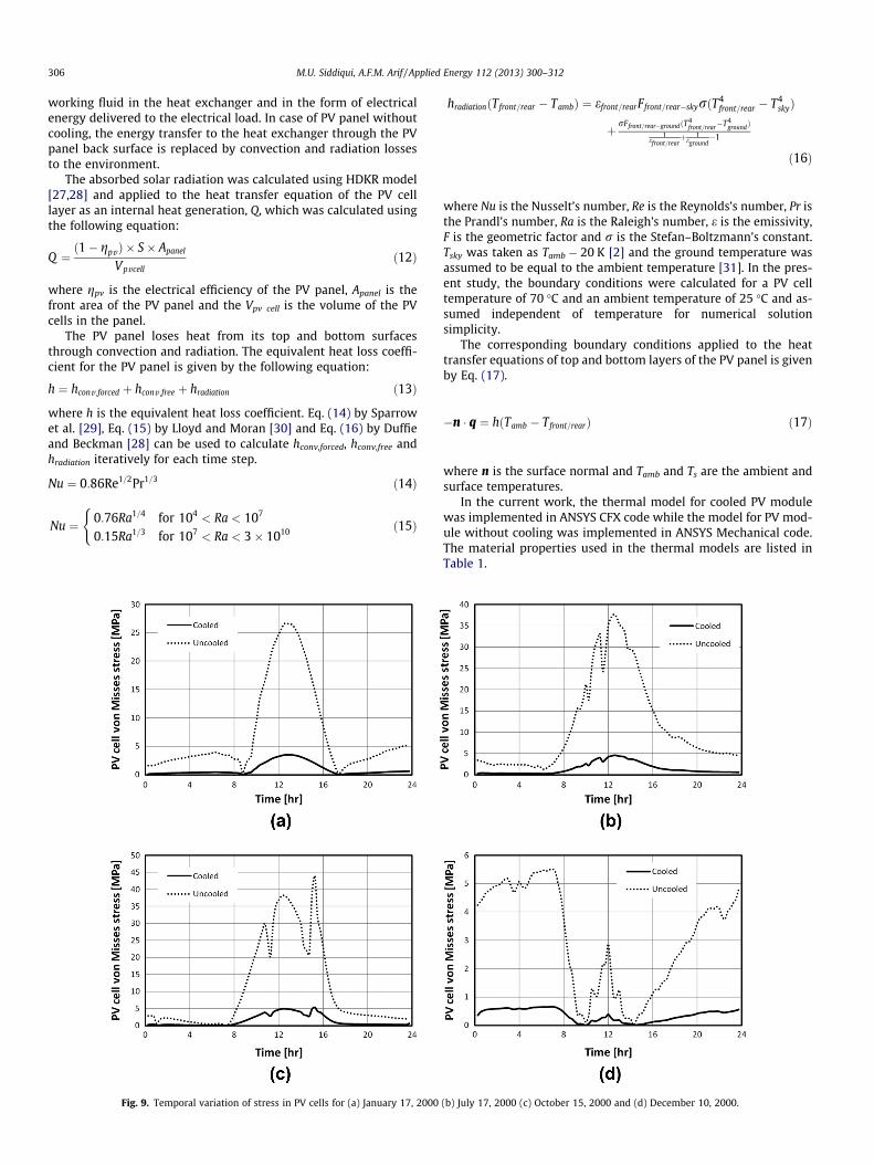
Fig. 9. Temporal variation of stress in PV cells for (a) January 17, 2000

hradiationðTfront=rear � TambÞ ¼ efront=rearFfront=rear�skyrðT4front=rear � T4

skyÞ

þ rFfront=rear�groundðT4front=rear�T4

groundÞ1

efront=rearþ 1

eground�1

ð16Þ

where Nu is the Nusselt’s number, Re is the Reynolds’s number, Pr isthe Prandl’s number, Ra is the Raleigh’s number, e is the emissivity,F is the geometric factor and r is the Stefan–Boltzmann’s constant.Tsky was taken as Tamb � 20 K [2] and the ground temperature wasassumed to be equal to the ambient temperature [31]. In the pres-ent study, the boundary conditions were calculated for a PV celltemperature of 70 �C and an ambient temperature of 25 �C and as-sumed independent of temperature for numerical solutionsimplicity.

The corresponding boundary conditions applied to the heattransfer equations of top and bottom layers of the PV panel is givenby Eq. (17).

�n � q ¼ hðTamb � Tfront=rearÞ ð17Þ

where n is the surface normal and Tamb and Ts are the ambient andsurface temperatures.

In the current work, the thermal model for cooled PV modulewas implemented in ANSYS CFX code while the model for PV mod-ule without cooling was implemented in ANSYS Mechanical code.The material properties used in the thermal models are listed inTable 1.

(b) July 17, 2000 (c) October 15, 2000 and (d) December 10, 2000.

Fig. 10. Paths for studying spatial distribution of temperature and stresses.

M.U. Siddiqui, A.F.M. Arif / Applied Energy 112 (2013) 300–312 307

2.3. Structural model

Finite element method was used to calculate the thermal stres-ses developing in the PV panel and two structural models wereimplemented [22,32]. Applying principle of virtual work underonly temperature body load gives,

fdugTZ

vol½B�T ½D�½B�dvfug ¼ fdugT

Zvol½BT �½D�fethgdv ð18Þ

Fig. 11. PV cell temperature (a) with

Since {du}T is an arbitrary displacement vector, the above equationreduces to,

½K�fug ¼ fFthg ð19Þ

where [K] =R

vol[B]T[D][B]dv is the element stiffness matrix; {Fth} = -Rvol[B]T[D]{eth}dv is the element thermal load vector; {eth} = {a}DT is

the thermal strain vector and {a} is the vector of coefficient of ther-mal expansion, [B] is the displacement gradient matrix, [D] is thematerial properties matrix and DT is the temperature differencefrom the reference condition.To calculate the thermal stressesdeveloping in the body, the Hooke’s law, given by Eq. (20), is used.

frg ¼ ½D�feg ð20Þ

where {r} is the stress vector and {e} is the elastic strain vectorequal to the difference of the total and thermal strains.

feg ¼ feTg � fethg ð21Þ

The structural model for PV panel without cooling was imple-mented in ANSYS Mechanical using SHELL181 layered structuralelements. The structural model for cooled PV panel was imple-mented in ANSYS Mechanical environment. Only the PV panelwas modeled for structural analysis using the same geometryand mesh as the thermal model. The finite element used was SO-LID185 which is a brick element defined by eight nodes having

cooling, and (b) without cooling.

Fig. 12. PV cell von Misses stress (a) with cooling, and (b) without cooling.

308 M.U. Siddiqui, A.F.M. Arif / Applied Energy 112 (2013) 300–312

three degrees of freedom at each node. Temperature distributioncalculated in the thermal analysis was applied to the model asbody load. To restrain the model structurally, the four corners ofthe model were fixed in all degrees of freedom.

The structural properties of all panel materials were assumed tobe temperature-independent linear-elastic and are shown in Table2. The strain-free temperature was assumed to be 25 �C which isthe standard test conditions (STC) cell temperature used in PVmodule datasheets.

2.4. Coupling thermal and electrical models

As shown by Eq. (12), the thermal and electrical performance ofPV panels are coupled together. As the PV cell temperature in-creases, efficiency decreases which then modifies the amount ofabsorbed energy heating the PV panel. During a transient analysis,this two-way coupling needs to be modeled in order to accuratelycalculate the correct temperature distribution in the panel. Toestablish a two-way coupling between electrical efficiency and celltemperatures, first an expression for temperature dependence ofelectrical efficiency, given by Eq. (22), was developed by differen-tiating the equation for efficiency with respect to temperature. It

was then used to calculate the electrical efficiency at each iterationusing Eq. (23).

@gpv

@Tcell¼ 1

Gref ApanelImp

@Vmp

@Tcellþ Vmp

@Imp

@Tcell

� �ð22Þ

gpv ¼ gpv ;ref 1�@gpv

@TcellðTcell;avg � Tcell;ref Þ

� �ð23Þ

where Tcell is PV cell temperature, Tcell,avg is the average cell temper-ature in the PV panel, G is the incident solar radiation, Apanel is thefront surface area of the PV panel and Imp and Vmp are the maximumpower point current and voltage.

Different methodologies were adopted to include this couplingin the thermal model for panels with and without cooling. Thethermal model for panel with cooling was developed in ANSYSCFX environment which employs an iterative solver to solvemomentum, continuity and energy equations. For the model of pa-nel without cooling, the above methodology cannot be employed.This is because ANSYS Mechanical FEA code, in which the modelwithout cooling has been implemented, does not use iterative sol-ver. Therefore, instead of using the PV cell temperature from thesame time step in Eq. (23), the cell temperature from the previoustime step was used. The flowchart of the coupling methodology isshown in Fig. 4.

3. Model validation

3.1. Validation of thermal model without cooling using experimentaldata

The thermal model for PV panel without cooling was validatedusing experimentally measured data for a 5940 Watts PV site usingSchott Solar SAPC-165 multi-crystalline silicon PV panel located atTallahassee, Florida, USA. The meteorological data and measuredPV back surface temperature for the PV site for 1 day (May 15,2005) was taken from the PV performance database maintainedby Florida Solar Energy Center. A comparison of the predicted PVback surface temperature by the thermal model and the measuredtemperature is shown in Fig. 5. The root mean square error in themodel prediction of panel back surface temperature was 4.9 �C.The correlation factor (r) was calculated to be 0.95.

3.2. Validation of thermal model with cooling using analytical model

The thermal mode with cooling was validated by comparing theaverage cell temperature and outlet fluid temperature predicted bythe thermal model at various fluid velocities with the temperaturespredicted by the analytical model for parallel channel heat exchan-ger PV/T collector presented by Sarhaddi et al. [6]. The results ofthe comparison are shown in Table 3. The root mean square errorsin the prediction of PV cells and outlet fluid temperatures were0.74 �C and 1.47 �C respectively.

3.3. Validation of electrical model using manufacturer suppliedexperimental data

The validation of the electrical model was carried out by com-paring the model predictions for the maximum power of PV mod-ules of various technologies with the values reported in the moduledatasheets. For six different modules and considering three differ-ent operating conditions, the root mean square errors (RMSE) andthe mean bias errors (MBE) in the maximum power predictionwere calculated and are reported in Fig. 6. As can be seen fromthe figure, all errors for 5 out of the six modules are less than1.5%. For the sixth module, the RMSE and MBE are 3% and 4%respectively.

Fig. 13. PV cell temperature and thermal stress along (a and b) path P1 (c and d) path P2 and (e and f) path T1.

M.U. Siddiqui, A.F.M. Arif / Applied Energy 112 (2013) 300–312 309

4. Results and discussion

Using the developed multi-physics model, the thermal, struc-tural and electrical performance of a crystalline silicon PV module(AstroPower AP-110) was simulated for 4 days with differentmeteorological conditions at Jeddah, Saudi Arabia. The ambienttemperature and total irradiance on a horizontal plane for the fourselected days is presented in Fig. 7. The total horizontal irradiancewas used to calculate absorbed solar radiation in the PV cells usingHDKR model. The absorbed radiation and the ambient temperaturewere used in the thermal model to calculate the temperature dis-tribution in the PV panel which was then used to calculate thestress distribution inside the panel. The electrical model used the

absorbed radiation and average PV cell temperature to calculatethe electrical power output and the electrical efficiency throughoutthe day. The electrical model parameters for the reference condi-tion are given in Table 4.

4.1. Temporal variation of PV cell temperature and thermal stresses

For all 4 days, the temporal variation of PV cell temperature andthermal stresses are shown in Figs. 8 and 9 respectively. Fig. 8a–dshow temporal variation of PV cell temperature at point T1 for thefour simulated days. For January 17, 2000, the maximum temper-ature occurred at 12:30 pm and was 61 �C for the panel withoutcooling and 31 �C for the cooled panel. For July 17, the maximum

Fig. 14. Variation of electrical power with time in PV panel with cooling for (a) January 17, 2000, (b) July 17, 2000, (c) October 15, 2000 and (d) December 10, 2000.

310 M.U. Siddiqui, A.F.M. Arif / Applied Energy 112 (2013) 300–312

cell temperature occurred at 12:30 and was 74.7 �C for panel with-out cooling and 33.1 �C for panel with cooling. For October 15, themaximum PV cell temperature occurred at 3:45 pm and was 84 �Cfor the panel without cooling and 35 �C for the cooled panel. ForDecember 10, the panel without cooling showed lower cell tem-perature through most part of the day. This is because the inletwater temperature for the heat exchanger cooling the PV panelwas set to 25 �C throughout the day. The maximum PV cell temper-ature occurred was 29 �C at 12:00 pm while it was 25.5 �C for thecooled panel.

The temporal variation of thermal stresses for the 4 days isshown in Fig. 9a–d. Because the strain-free temperature was as-sumed to be 25 �C, the von Misses stress showed zero magnitudewhen the PV cell temperature equaled 25 �C. For January 17, themaximum von Misses stress for the panel without cooling was27 MPa and for the cooled panel was 3.5 MPa. For July 17, the cor-responding maximum von Misses stress values for the panel with-out cooling and with cooling were 38 MPa and 4.6 MParespectively. For October 15, the maximum stress in the PV cellswas 44 MPa for the panel without cooling and 5 MPa for the cooledpanel. Finally, for December 10, the maximum stress was 5.5 MPafor the panel without cooling and 0.7 MPa for the cooled panel.

4.2. Spatial distribution of PV panel temperatures and thermal stress

For studying the spatial temperatures and stresses, initially1 day was studied in detail. Three paths were defined along thePV panel. Paths P1 was along the length of the panel, path P2was along the panel’s width and path T1 was across the thicknessof the panel starting from the bottom. All paths are shown inFig. 10. The day selected for the detailed study was July 17, 2000because of its high and uniformly distributed solar irradiance andhigh ambient temperatures. For the time 12:30 when the PV cell

temperature and stresses were maximum, the PV cell temperatureand von Misses stress in the PV panels with and without coolingare shown in Figs. 11 and 12.

The spatial variation of temperature and stresses were plottedalong the three paths shown in Fig. 10 and are shown in Fig. 13.Fig. 13a and c show the PV cell temperature variation along pathsP1 and P2 in the panel with and without cooling. The figures showthat the PV cell temperature for PV panel without cooling showedalmost constant values along the paths with cyclic variation within0.2 �C. On the other hand, the cell temperature for cooled PV panelshowed almost 5 �C rise along paths P1 and 2 �C rise along pathsP2. The non-uniformity of cell temperatures in the cooled panelwas due to non-uniform flow in the heat exchanger.

Fig. 13b and d shows the variation of von Misses stress in PVcells along paths P1 and P2. In the figures, stress values for the firstand the last cells include the effect of the applied boundary condi-tion and the effect will increase as the path is moved closer to theboundary. Along, the paths, the panel without cooling showedsymmetric variation in stress with von Misses stresses around35 MPa. The cooled panel showed one order of magnitude lowerstress values (around 1 MPa) with a gradual increase in the stressalong the path due to the increase in the cell temperature. In thepanel without cooling there was also a strong stress gradient be-tween the cells but the stress gradient dropped significantly forthe cooled panel.

Fig. 13e shows the temperature variation across the thickness ofthe PV panel at location T1. It shows that PV panels with and with-out cooling have different types of variation along the thickness ofthe panel. For the panel without cooling, the temperature variedbetween 73.6 �C and 74.7 �C with the minimum temperature beingat the top where the convection losses were maximum. For the pa-nel with cooling, the temperature varied between 30 �C and 33.1 �Cwith the minimum temperature being at the bottom where the

M.U. Siddiqui, A.F.M. Arif / Applied Energy 112 (2013) 300–312 311

heat exchanger is attached. The von Misses stress variation acrossthe thickness is shown in Fig. 13f. The figure shows no significantstresses developing in the encapsulent layer due to the very lowelastic modulus of the encapsulent material. For panels with aswell as without cooling, the maximum stresses occurred in thePV cell layer (37.5 MPa for the panel without cooling and4.6 MPa for the cooled panel).

4.3. Temporal variation of electrical performance

Using the measured irradiance and the average predicted PVcell temperature, the electrical performance of a crystalline siliconmodule with and without cooling was simulated for the conditionsof the 4 days considered in this study. The electrical power outputof the PV module for the 4 days is shown in Fig. 14 and the varia-tion of electrical efficiency is shown in Fig. 15. For the 3 days (Jan-uary 17, 2000, July 17, 2000 and October 15, 2000) in which thedifference between the PV cell temperature of panel with andwithout cooling was high, there is marked improved in the electri-cal performance of the PV panel as shown by Fig. 14a–c. ForDecember 10, 2000, the maximum difference in PV cell tempera-tures of panels with and without cooling at any time during theday was 6 �C. Within this temperature difference range, the electri-cal performance of the PV panel shows no appreciable variation.

Fig. 15 shows variation of electrical efficiency with time duringthe 4 days considered in this study. As expected, the cooled PVpanels showed higher efficiencies than the panels without coolingfor the 3 days with higher difference between cooled and uncooledcell temperatures (January 17, 2000, July 17, 2000 and October 15,2000) as shown in Fig. 15a–c. For December 10, 2000, the two pan-els show same efficiency throughout the day.

Fig. 15. Variation of electrical efficiency with time in PV panel with cooling (a) Janua

Fig. 15 also sheds light on the dependence of electrical effi-ciency upon irradiance and cell temperature. In general, increasingirradiance increases efficiency while increasing PV cell tempera-ture decreases it. At low irradiance, the influence of irradiance ishigher but as the cell temperature increases, the positive effect ofincreasing irradiance decreases until eventually the efficiencystarts to drop with increasing cell temperature. This phenomenonis visible in Fig. 15a–c. During morning and evening, the efficiencyincreased with increasing irradiance. During the peak sunshinehours, the panel with cooling showed slight decrease in efficiencydespite the increasing irradiance while the efficiency of the cooledpanel completely followed the trend of irradiance.

5. Conclusions

In this paper, the implementation of a multiphysics model forthe thermal, electrical and structural performance prediction ofPV modules is presented. The developed multiphysics model wasused to simulate the thermal, structural and electrical performanceof a PV module for 4 days representing four different types of envi-ronmental conditions at Jeddah, Saudi Arabia. From the study, thefollowing conclusions were drawn.

� The effectiveness of cooling in improving the electrical conver-sion efficiency is more strongly dependent on irradiance thanambient temperature. For example, January 17, 2000 andDecember 10, 2000 showed similar ambient temperatures(around 20–25 �C) but the incident radiation was much lowerfor December 10, 2000 (less than 350 W). Therefore, the cooledpanel provided around 20 W more power than the uncooledpanel on January 17, 2000 while there was no performanceimprovement for December 10, 2000.

ry 17, 2000, (b) July 17, 2000, (c) October 15, 2000 and (d) December 10, 2000.

312 M.U. Siddiqui, A.F.M. Arif / Applied Energy 112 (2013) 300–312

� The cooled panel showed lower cell temperatures than theuncooled module as expected but the temperature gradientsin the cooled panel were also higher (4.5 �C along path P1).� The cooled panel showed one order of magnitude lower stress

level than the uncooled panel. The maximum stress along pathP1 was 1 MPa for the cooled panel while it was 35 MPa for theuncooled panel.� The results shows that the modeling methodology presented in

the current work may be used to develop simple correlations todecide correct heat exchanger operating conditions as a func-tion of irradiance, ambient temperature, wind speed, etc.

Acknowledgements

The authors would like to acknowledge the support of KingFahd University of Petroleum and Minerals through the Centerfor Clean Water and Clean Energy at KFUPM (DSR project # R6-DMN-08) and MIT.

References

[1] Skoplaki E, Palyvos JA. On the temperature dependence of photovoltaic moduleelectrical performance: a review of efficiency/power correlations. Sol Energy2009;83:614–24.

[2] Jones AD, Underwood CP. A thermal model for photovoltaic systems. SolEnergy 2001;70:349–59.

[3] King DL, Boyson WE, Kratochvil JA. Photovoltaic array performancemodel. Albuquerque, New Mexico: Sandia National Laboratories; 2004.

[4] Acciani G, Falcone O, Vergura S. Analysis of the thermal heating of poly-Si anda-Si photovoltaic cell by means of FEM. In: International conference onrenewable energies and power quality; 2010.

[5] Tiwari A, Sodha MS. Performance evaluation of solar PV/T system: anexperimental validation. Sol Energy 2006;80:751–9.

[6] Sarhaddi F, Farahat S, Ajam H, Behzadmehr A, Mahdavi Adeli M. An improvedthermal and electrical model for a solar photovoltaic thermal (PV/T) aircollector. Appl Energy 2010;87:2328–39.

[7] Amori KE, Taqi Al-Najjar HM. Analysis of thermal and electrical performance ofa hybrid (PV/T) air based solar collector for Iraq. Appl Energy 2012;98:384–95.

[8] Amrizal N, Chemisana D, Rosell JI. Hybrid photovoltaic–thermal solarcollectors dynamic modeling. Appl Energy 2013;101:797–807.

[9] Teo HG, Lee PS, Hawlader MNA. An active cooling system for photovoltaicmodules. Appl Energy 2011;90:309–15.

[10] Usama Siddiqui M, Arif AFM, Kelley L, Dubowsky S. Three-dimensional thermalmodeling of a photovoltaic module under varying conditions. Sol Energy2012;86:2620–31.

[11] Huang BJ, Lin TH, Hung WC, Sun FS. Performance evaluation of solarphotovoltaic/thermal systems. Sol Energy 2001;70:443–8.

[12] Hishikawa Y, Imura Y, Oshiro T. Irradiance-dependence and translation of theI–V characteristics of crystalline silicon solar cells. In: Photovoltaic SpecialistsConference (PVSC), 2000 28th IEEE, 2000; p. 1464–7.

[13] Marion B, Rummel S, Anderberg A. Current–voltage curve translation bybilinear interpolation. Prog Photovoltaics Res Appl 2004;12:593–607.

[14] DeSoto W, Klein SA, Beckman WA. Improvement and validation of a model forphotovoltaic array performance. Sol Energy 2006;80:78–88.

[15] Boyd MT, Klein SA, Reindl DT, Dougherty BP. Evaluation and validation ofequivalent circuit photovoltaic solar cell performance models. J Sol Energy Eng2011;133:021005.

[16] Villalva MG, Gazoli JR, Filho ER. Comprehensive approach to modeling andsimulation of photovoltaic arrays. IEEE Trans Power Electron2009;24:1198–208.

[17] Siddiqui MU. Multiphysics modeling of photovoltaic panels and arrays withauxiliary thermal collectors. King Fahd University of Petroleum & Minerals;2011.

[18] Eitner U, Altermatt PP, Köntges M, Meyer R, Brendel R. A modeling approach tothe optimization of interconnects for back contact cells by thermomechanicalsimulations of photovoltaic modules. In: 23rd European photovoltaic solarenergy conference, Valencia, Spain, vol. 54; 2008. p. 258–60.

[19] Gonzalez M, Govaerts J, Labie R, De Wolf I, Baert K. Thermo-mechanicalchallenges of advanced solar cell modules. In: 12th international conferenceon thermal, mechanical and multiphysics simulation and experiments inmicroelectronics and microsystems, EuroSimE 2011; 2011. p. 1–7.

[20] Meuwissen M, Van Den Nieuwenhof M, Steijvers H. Simulation assisted designof a PV module incorporating electrically conductive adhesive interconnects.In: 21st European photovoltaic solar energy conference and exhibition,Dresden, Germany; 2006. p. 2485–90.

[21] Dietrich S, Pander M, Sander M, Schulze SH, Ebert M. Mechanical andthermomechanical assessment of encapsulated solar cells by finite-element-simulation. In: Dhere NG, Wohlgemuth JH, Lynn K, editors. Reliability ofphotovoltaic cells, modules, components, and systems III, vol. 7773, SPIE;2010, p. 77730F1–10.

[22] Siddiqui MU, Arif AFM. Effect of changing atmospheric and operatingconditions on the thermal stresses in PV modules. ESDA 2012 vol. 2, NantesFrance. American Society of Mechanical Engineers; 2012, p. 729–40.

[23] Siddiqui MU, Arif AFM, Bilton AM, Dubowsky S, Elshafei M. An improvedelectric circuit model for photovoltaic modules based on sensitivity analysis.Sol Energy 2013;90:29–42.

[24] Duffie JA, Beckman WA. Solar engineering of thermal processes. 2nd ed. NewYork: John Wiley & Sons, Inc.; 1991.

[25] Incropera FP, DeWitt DP. Fundamentals of heat and mass transfer. 4th ed. JohnWiley & Sons, Inc.; 1996.

[26] Wilcox DC. Turbulence modeling for CFD. 2nd ed. DCW Industries; 1998.[27] Reindl DT, Beckman WA, Duffie JA. Evaluation of hourly tilted surface radiation

models. Sol Energy 1990;45:9–17.[28] Duffie JA, Beckman WA. Solar engineering of thermal processes. 3rd

ed. Hoboken, New Jersey: John Wiley & Sons, Inc.; 2006.[29] Sparrow EM, Ramsey JW, Mass EA. Effect of finite width on heat transfer and

fluid flow about an inclined rectangular plane. ASME J Heat Trans 1979;101:2.[30] Lloyd JR, Moran WP. Natural convection adjacent to horizontal surface of

various platforms. ASME J Heat Trans 1974;96:443.[31] Armstrong S, Hurley WG. A thermal model for photovoltaic panels under

varying atmospheric conditions. Appl Therm Eng 2010;30:1488–95.[32] Hasan O, Arif AFM, Siddiqui MU. Finite element modeling and analysis of

photovoltaic modules. IMEC 2012, Housten, Texas: American Society ofMechanical Engineers; 2012. p. 1–10.