electrical & computer engineering & computer engineering. ... which are the bottleneck in...

VLSI Component Placement byGrid Warping

Zhong Xiu

2003

Advisor: Prof. Rutenbar

Electrical & ComputerENGINEERING

VLSI Component Placement by GridWarping

Zhong Xiu

A thesis submitted to the graduateschool in partial fulfillment of the

requirements of the degree of

Master of ScienceIn

Electrical and Computer Engineering

Carnegie Mellon UniversityPittsburgh, Pennsylvania 15213

May 2003

Abstract

Placement is an important step in the overall IC design process in DSM technologies, as

it defines the on-chip interconnects, which are the bottleneck in determining circuit

performance. The "quadratic placement" methodology is reputedly used in many

commercial and in-house tools for placement of standard-cell and gate-array designs.

Numerous quadratic placement algorithms have been developed and tested over time.

Currently, these methods are capable of placing a few million modules, but are unable to

scale beyond that. The legalization step, required of all algorithms, is the step that is

expensive to perform and has limited scalability.

We have extended and improved an algorithm specifically targeting these extremely large

placement problems. Our approach is fundamentally different than existing tools in that

we move the placement area as opposed to moving the modules, thereby formulating a

problem that is mainly dependent on the placement area, instead of the net list size. As a

result, our algorithm is essentially a low dimensional optimization problem that is

inherently parallel. Preliminary tests running on big benchmarks show that our algorithm

is extremely scalable and will potentially allow us to handle the ever-increasing net list

better than existing tools. We believe we can improve our placement algorithm with more

future work.

VLSI Component Placement by Grid Warping i

Acknowledgments

I would like to thank my advisor, Rob A. Rutenbar, for his guidance throughout this

research project. He has been an unlimited source of information and ideas, not only for

my research but also for the final writing of this thesis. He not only pointed out the

direction, but also discussed many details with me.

I would like to thank Larry Pileggi for having reviewed this thesis.

I would also like to thank James Ma for cooperating with me during the implementation

of this project. His intelligent ideas and diligent work are appreciated.

I would like to thank Suzanne Fowler for allowing me to use her original codes. I would

also like to thank Trevor Carlson for his work on the IO part of this project.

Finally I would like to thank my father and mother. Without their consistent supports, I

could achieve nothing.

VLSI Component Placement by Grid Warping ii

Table of Contents

1 Introduction............................................ 11.1 The Problem ............................................................... 11 2 Background .......................... 21 3 Motivation ............................... 31.4 Organization of the Thesis ......................................... 3

2 Previous Work........................................ 52.1 Basic Quadratic Formulation ...................................... 52.2 Quadratic Solver ......................................................... 62.3 Refine Step ................................................................. 8

2.3.1 PROUD ............................................................................ 82.3.2 GORDIAN ....................................................................... 92.3.3 GORDIANL ................................................................... 102.3.4 DOMINO ....................................................................... 112.3.5 Other Techniques ........................................................... 13

2.4 Summary ................................................................. 15

VLSI Component Placement by Grid Warping iii

3 Approach: Grid Warping ................... 163.1 Overview .................................................................. 163.2 Initial Placement ....................................................... 173.3 Warping .................................................................... 193.4 Structure of Grid ...................................................... 25

3.4.1 Source Grid ..................................................................... 253.4.2 Target Grid ...................................................................... 27

3.5 Optimization ............................................................. 303.5.1 Classical Powell-style Optimization ............................... 303.5.2 Evaluation of the Cost Function .................................... 323.5.3 Iterative Sequential Warping ......................................... 34

3.6 Final Legalization ..................................................... 353.7 Summary .................................................................. 36

4 Experimental Results........................... 374.1 Experimental Methodology ...................................... 374.2 Results and Analysis ................................................ 384.3 Summary .................................................................. 41

5 Conclusions........................................... 445.1 Summary ................................................................. 445.2 Direction ................................................................... 44

VLSI Component Placement by Grid Warping iv

Introduction

1.1 The Problem

In a VLSI CAD flow, physical design is a backend process. In the physical

implementation of deep-submicron ICs, placement solution quality is a major

determinant of whether timing correctness and routing completion will be achieved. In

row-based placement, the first-order objective has always been obvious: place connected

cells closer together so as to reduce total routing and lower bounds on signal delay.

Because there are many layout iterations, and because fast placement estimation is

needed in floorplanning for design convergence, a placement tool must be extremely fast.

As instance sizes grow larger, swap-based methods like annealing may be too slow

except for detailed placement improvement. Due to its speed and "global" perspective,

quadratic placement is reputedly an approach that has been used within commercial tools

for placement of standard-cell and gate-array designs.

Quadratic placement algorithm makes two basic assumptions: 1) Each module is modeled

as a dimensionless point; 2) Each net is modeled as a set of 2-point springs. With these

two assumptions, the placement problem can be easily formulated as a neat mathematical

problem, and this problem can be solved relatively quickly even for very large net-lists.

But, since every module has its own shape and size, unfortunately the placement is illegal

with many overlaps. So a legalization step is needed. This step varies among tools, but it

is this step that is expensive and not able to scale very well. Today, most tools adopt a

partition-based approach as the legalization step. These tools can typically manage up to

a few million modules. But they all become very slow for larger designs.

VLSI Component Placement by Grid Warping 1

Introduction

1.2 Background

Today, all layout flows are composed of several heterogeneous steps: logic synthesis,

placement, global routing, and timing analysis are intermixed. A sequence of coarse to

fine layouts is evolved to allow difficult constraints to be addressed either logically or

physically at each step. But no matter how this flow is designed, the placement of a

single flat net list under basic area, congestion, and delay constraints is a core

competency. Placer capacity and quality are enormously important in all layout flows.

One important component of recent flows is the capability to "finalize" a "near" layout

efficiently.

Most layout tools adopt the fiat style of placement design. These tools can typically

manage up to a few million modules. Larger designs are forced to resort to a hierarchical

approach. The majority of these flat style tools use a quadratic placement method. There

are many existing placement tools using quadratic placement as the starting point. But

they tend to deviate in the way of legalizing the placement.

Some famous placement algorithms: PROUD [1], GORDIAN [2], GORDIANL [3], etc,

all use a classical quadratic objective function to begin placement, and alternate quadratic

solves with partitioning. They use partitioning to reduce the size of the placement

problem. Each region is recursively cut and the quadratic algorithm applied until each

region has a small number of modules. The resulting placements of these placers are not

legal. So they still use some strategies in the end to produce a legal placement.

Overall, these partition-based placers are very fast and the resulting placement quality is

very good, even competitive to simulated annealing. But they are very slow when dealing

with very large designs. And actually this is a common problem for most current tools,

including placers that use other strategies.


Introduction

1.3 Motivation

In [20], Fowler developed a fundamentally different concept for a placement scheme,

motivated in part by a desire to handle extremely large placements in a completely flat

way. Our work begins here, by trying to extend her very simple, first generation

formulation, and repair several flaws in this initial attempt. Similar to current tools, our

technique uses a quadratic placement method, but is fundamentally different when

attacking the legalization step. The idea is strikingly simple: rather than move the

gates/blocks to optimize their location, we elastically deform a model of the 2-D chip

surface on which the objects have been quickly and coarsely placed. Put simply: we

move the grid, not the gates. Rather than move each point, we "stretch" the underlying

sheet until the points arrange themselves to our liking.

This strategy has two potential advantages: (1) deforming the elastic sheet is

surprisingly simple, low-dimensional optimization; (2) this very big design problem

transformed from a very high-dimensional optimization task into a very large numerical

cost function with a small number of degrees of freedom that determine the warping of

the grid. But this large cost function can be evaluated on a network of cheap computers--

the problem is very parallel, unlike classical placers. Following [20], we call this method

placement by grid warping.

Because our placement algorithm is a very low dimensional problem, we believe that this

can be extremely scalable and therefore potentially useful in placing large net-lists.

1.4 Organization of the Thesis

Chapter 2 is a review of related previous work, serving as a background to some

placement techniques. Chapter 3 goes through our new reformulation idea of the grid

warping idea for placement, including initial quadratic placement followed by refinement


Introduction

steps. Chapter 4 describes the experiments we preformed and the results we obtained.

And Chapter 5 concludes with the future direction of this research.


2 Previous Work

In this chapter we will revisit the quadratic placement algorithm and review some

existing placement tools relevant to our work. Quadratic wire length objective functions

are very common in these tools. These tools start from the quadratic placement and try

bard to make it legal or bring it closer to a legal placement. Overlap removal is iteratively

performed in the refine step.

2.1 Basic Quadratic Formulation

A VLSI circuit is represented for placement by a weighted hyper-graph, with n vertices

corresponding to modules (vertex weights equal module areas), and hyper-edges

corresponding to signal nets (hyper-edge weights equal criticalities and/or multiplicities).

The two-dimensional layout region is represented as an array of legal placement

locations. Placement seeks to assign all cells of the design onto legal locations; such that

no ceils overlap and chip timing and routability are optimized. The placement problem is

a form of quadratic assignment; most variants are NP-hard. [4]

"Pad" constraints fix the locations of certain vertices (due to the pre-placement of I/O

pads or other terminals); all other vertices are movable. The one-dimensional placement

problem seeks to place movable vertices onto the real line so as to minimize an objective

function that depends on the edge weights and the vertex coordinates.

By modeling each module as a dimensionless point and each wire as 2-point springs, the

placement problem is transformed into a mathematical problem. Actually the two-

dimensional placement problem is addressed by the means of independent horizontal and

vertical placements. Each placement tries to minimize a quadratic matrix form.


Previous Work

Squared Wire Length Formulation: Minimize the objective ~(x) Y, i>j aij (xi - xj 2

subject to constraints Hx = b. This function can be rewritten as qb(x) = 1A xTQx.

(Here, xi is the x coordinate of module i, aij is the number of connections between module

i and module j)

If we take the pads constraints into consideration, the squared wire length formulation

can be written as:

tI)(x) = 1/2 xTQx + (1)

which is also a quadratic matrix form. (The formulation of Q and d can be found in [1]

[21)

fixed

Figure 1. Quadratic Formulation - For this example, the quadratic wire length in x-axis is:

I(Xl - k)2 + l(xa - XI)2 + (h - x2) 2 = [xi 2 - 2XlX2 + X22] + [-2k xl -2h X2] + [k 2 + h2]

The vast majority of quadratic placers solve the 2-dimensional placement problem with a

top-down approach. After the quadratic placement, the chip is divided into two parts and

quadratic placement algorithm is re-applied to each region, and this process recursively

repeats until each sub-region only has a small number of modules.

2.2 Quadratic Solver

To minimize (1), we compute the derivative of ~(x):

¯ ’(x) = Y2 xTQ + ~/2 Qx + d (2)

Since Q is a symmetric and positive definite matrix, (2) can be written as:

~’(x) = Qx + (3)


Previous Work

The optimal solution is: Qx = -d, which is a linear equation. Since the number of

modules can be millions, it is not practical to solve this equation directly. Iterative

methods are used to get the solution.

Iterative methods for solving large systems of linear equations can be classified as

stationary or non-stationary. Stationary methods include Jacobi, Gauss-Seidel,

Successive Over-relaxation (SOR) and Symmetric Successive Over-relaxation (SSOR).

They are older, easier to implement and computationally cheaper per iteration. Non-

stationary methods include Conjugate Gradient (CG), Generalized Minimal Residual

(GMRes) and numerous variations. These are relatively newer and notably harder

implement and debug, but provide for much faster convergence. Additional

computational expense per iteration is normally justified by much smaller numbers of

iterations. [4]

A difficulty associated with the SOR, Chebyshev semi-iterative, and related methods is

that they depend upon parameters that are sometimes hard to choose properly. CG is a

method without this difficulty for the symmetric positive definite Ax = b problem.

The essential idea of CG is: if the search directions are linearly independent and Xk solves

the problem

min(4)

x xo + span {Pl,’",

for k - 1, 2, ..., (here ~(x) = V2 xTAx - ba’x, p~, ..., pk are the k directions to search

minimal x) then convergence is guaranteed in at most n steps. This is because xn

minimizes q~(x) over n and therefore satisfies Ax,~ -- b.

The CG method can guarantee to find the accurate solution in at most n steps by choosing

the search directions that are so-called A-orthogonal, a detailed description of CG and

pre-conditioned CG can be found in [5] and [6].


Previous Work

2.3 Refine Step

As we know, after the quadratic placement algorithm, the layout has many overlaps.

There are different ways to remove the overlaps, and these lead to many different

placement algorithms. Most of these algorithms choose a recursive strategy to legalize

the layout. Algorithms using rain-cut partitioning are very popular. We will review some

famous placers and their refining strategies. These tools represent state of the art

quadratic placement placers.

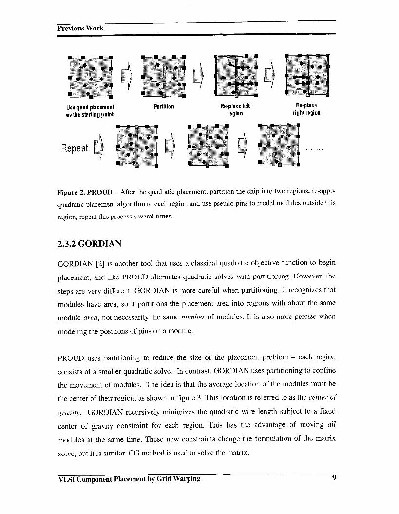
2.3.1 PROUD

PROUD [1] uses a direct quadratic placement as a starting point for a recursive min-cut

partitioning strategy. Once the initial placement is found, the placement area is cut into

two regions of about equal modules. The quadratic placement algorithm is re-applied to

the two resulting regions. Pseudo-pins on the cut line between the modules are used to

model connections with modules outside of the current region. Each region is recursively

cut and the quadratic algorithm applied until each region has only 10’s of modules. The

whole process is repeated three to five times so that the modules’ movements in one

region have a chance to globally affect all other regions. The process is illustrated in

figure 2.

The resulting placement is not legal, so PROUD finalizes the placement by snapping the

modules into rows. This alone would not produce a very good result, so it iteratively

looks at a small area (window) of the layout and swaps modules, using a greedy

algorithm, to improve wire length. Overall this algorithm is fairly fast, but it is interesting

to note that over half the total wire length improvements are due to this finalization step.


Previous Work

Use quad placement Padition Re-place left Re-placeas the starting point region right region

Repeat

Figure 2. PROUD - After the quadratic placement, partition the chip into two regions, re-apply

quadratic placement algorithm to each region and use pseudo-pins to model modules outside this

region, repeat this process several times.

2.3.2 GORDIAN

GORDIAN [2] is another tool that uses a classical quadratic objective function to begin

placement, and like PROUD alternates quadratic solves with partitioning. However, the

steps are very different. GORDIAN is more careful when partitioning. It recognizes that

modules have area, so it partitions the placement area into regions with about the same

module area, not necessarily the same number of modules. It is also more precise when

modeling the positions of pins on a module.

PROUD uses partitioning to reduce the size of the placement problem - each region

consists of a smaller quadratic solve. In contrast, GORDIAN uses partitioning to confine

the movement of modules. The idea is that the average location of the modules must be

the center of their region, as shown in figure 3. This location is referred to as the center of

gravity. GORDIAN recursively minimizes the quadratic wire length subject to a fixed

center of gravity constraint for each region. This has the advantage of moving all

modules at the same time. These new constraints change the formulation of the matrix

solve, but it is similar. CG method is used to solve the matrix.


Previous Work

x center x center

Figure 3. GORDIAN - Center of Gravity Constraints: The average location of the modules must

be the center of their region

The resulting placement is not legal either, so GORDIAN also does a finalization step.

For standard cells, GORDIAN only snaps them into rows. This is fast, but not very

effective. For macro-cells, GORDIAN performs an exhaustive slicing optimization.

Actually there are still many additional engineering and tuning optimizations to improve

the layout quality. Overall GORDIAN is a very competitive and fast algorithm.

2.3.3 GORDIANL

Some researchers [3] noted the pros and cons of using a quadratic objective function.

These types of functions tend to overweight long wires at the expense of shorter ones.

(See figure 4 for a simple example) In other words, quadratic objectives functions

minimize the squared Euclidean length of all nets rather than just the standard Manhattan

length of all nets. The reason these functions have become so popular is that they are

continuously differentiable and minimizing them only requires solving a linear system of

equations. But this is not true for linear objective functions.


Previous Work

fixed movable fixeds) quadratic objective function

le fixedb) line~.r objective function

Figure 4. GORDIANL - Optimal placements for different objectives: two fixed modules A, C

and a movable module B. Three nets connect them. Minimizing the quadratic objective function

yields the placement in a). The minimization of the linear function results in the placement in b).

This figure is from [3].

To obtain a near linear wire length estimation, GORDIANL uses essentially the same

algorithm as GORDIAN, except that after each quadratic solve it calculates the linear

wire length of each net and uses the inverse lengths as weights for the next quadratic

solve. This process is repeated until the wire length converges. By solving a sequence of

modified quadratic wire length problems, the resulting placement approaches a linear

wire length model without any difficult linear programming.

As they mentioned in the paper, GORDIANL yields results with up to 20% less area than

the quadratic objective function of the original GORDIAN procedure. The main reason

for these distinct improvements, as they said, is the length reduction of nets connecting

only two and three pins. But GORDIANL needs a much longer time to converge than

GORDIAN.

2.3.4 DOMINO

One detailed placer that is commonly used in conjunction with GORDIAN and

GORDIANL to further improve the layout is DOMINO [7] [8]. DOMINO is an efficient

iterative improvement procedure for row-based cell placement with special emphasis on

the objective function used to model net lengths. This iterative placement process starts

with a given placement and produces a sequence of intermediate placements. DOMINO


Previous Work

is able to iteratively improve already legal placements, or legalize placements containing

overlapping modules, by cleverly formulating the problem into a network flow problem.

In the first step, an initial placement is generated by the GORDIAN or GORDIANL

procedure. DOMINO uses these coordinates as initial placement for the iterative process.

In each iteration step a new placement is generated from a current placement. The

process finishes when after several generations no significant improvement is achieved.

To divide each generation into local subproblems, the layout area is covered by an array

of overlapping regions. A subproblem consists of rearranging the cells currently placed

inside a region. Since the cells have different heights, their rearrangement may produce

overlaps and unused spaces. To construct a legal placement, DOMINO uses a simple but

effective strategy as briefly described below.

border l~se

Figure 5. DOMINO - Generation of a new placement: this figure is from [8].

DOMINO walks the layout along a jagged borderline (see figure 5). It tries to legalize

and improve the modules immediately above this line by packing them into rows. It

attempts to reduce the wire length with minimal disturbance to the modules. After each

iteration, a new, improved placement is generated that is free of interspersed spaces and

overlapping modules. These one-dimensional placement improvements "walks" are


Previous Work

iterated over the whole layout until no significant improvement can be found. DOMINO

is a fast, efficient, detailed placer with the added advantage of being deterministic.

2.3.5 Other Techniques

PROUD, GORDIAN and GORDIANL all use some forms of rain-cut partitioning to

spread out dense overlapping modules. DOMINO is a deterministic detailed placer. We

now turn our focus to two placers using two very different techniques to accomplish the

same goal.

KRAFTWERK:

The fundamental problem with the quadratic formulation, according to [9], is it only

models wires as attractive forces. So they present a new force directed method for global

placement. Besides the well-known wire length dependent forces they use additional

forces to reduce cell overlaps and to consider the placement area. They believe that

compared to existing approaches, the main advantage is that the algorithm provides

increased flexibility and enables a variety of demanding applications.

A standard quadratic solve is first calculated. Then each small region of the placement

area is given an attractive or repulsive force that acts on every module - an attractive

force for regions with excess modules and a repulsive force for regions with excess

space. For each module, a net force is calculated and a new quadratic solve is formulated

with these new constraints. This process is repeated until the wire length converges.

The final placement is again not legal, and they choose to use DOMINO to finish the

layout. Based on their results, they said that this placer is able to outperform

GORDIAN/DOMINO in placement area by 6% using comparable or less CPU time.

They emphasized that the algorithm is the first one that is able to handle large mixed

block/cell placement problems without treating blocks and cells differently. And contrary

to state-of-the-art approaches, this algorithm can assure that timing requirements are

precisely met. Its main advantage may be due to the elimination of rain-cut partitioning;


Previous Work

without partitioning it is impossible for the tool to make bad decisions, forcing modules

to reside in sub-optimal regions. One problem when applied to large net-lists, however, is

the reportedly complicated force calculation and tuning process for each module.

VYGEN:

The final tool we will discuss is a tool by Vygen [10]. They strongly believe that the

initial quadratic placement is a good placement and the only problem is that modules

overlap. So the basis of their algorithm is a quadratic optimization approach combined

with a new quadrisection algorithm. In contrast to most previous quadratic placement

methods, no rain-cut objective is used at all. Based on a quadratic placement, a

completely new algorithm finds a four-way partitioning meeting capacity constraints and

minimizing the total movement. Their solution is to legalize the quadratic placement with

as little movement as possible. They accomplish this by partitioning the layout into four

sub-regions (a 2x2 grid) based only on a capacity constraint. Their capacity constraint

the total area of modules that is allowed in a particular region. The process continues

refining the placement area into a 4x4 grid, then 8x8, and so on, until it is sufficiently

fine. At each stage, the circuits are assigned to the rectangular regions induced by the

grid. The procedure stops when the grid is fine enough: The height of the rows equals the

standard height of the circuits, and the width of the columns is roughly 50 times the

minimum width of a circuit. A special algorithm does the final detailed placement.

The final placement procedure makes use of the row structure of a standard cell chip. The

final placement consists of two main phases. The first phase determines an assignment of

the non-fixed circuits to the zones such that the total width of the circuits assigned to one

zone does not exceed the width of this zone. The second phase of the final placement

then finds an optimum disjoint placement such that the circuits remain within their zones

and also remain in their horizontal order according to the positions after the last QP. In

this way, they mentioned that they were able to legally place a 200,000 net circuit in

about six hours.


Previous Work

2.4 Summary

All tools discussed above agree that a quadratic placement is a good start, if nothing else.

The differences arise when tying to legalize this initial quadratic placement. Many apply

a recursive min-cut partitioning algorithm to spread the modules out across the placement

area, while others believe this may force modules to wrongly live in sub-optimal regions.

Most descendants of GORDIAN use some form of linear re-weighting to better

approximate Manhattan instead of quadratic wire length. Except [10], who argues for a

"pure" quadratic placement, and strives to preserve as much of this placement as possible

in his own legalization process.

While these tools are relatively fast and efficient when dealing with wire length, we

believe problems will become apparent when trying to place extremely large net-lists.

The above algorithms, maybe with the exception of [10], were developed to target

placements of tens of thousands of modules. With transistors shrinking and density of

chips increasing, the need for a very large fiat placer is growing dramatically.


3 Approach: Grid Warping

3.1 Overview

From Chapter 2, we know that there are two basic steps in placement algorithms: (1)

obtain an initial placement and (2) refine this placement until it is legal, or close to legal.

The main differences in the algorithms appear in the refinement step. Currently these

algorithms move the modules to legalize their locations. Here is where our placement

technique is fundamentally different. Instead of moving the modules, we move, or warp,

the surface on which these modules are placed. By creating a two-dimensional grid on

top of this surface, we are able to warp this grid until the underlying modules are

arranged such that our cost function is minimized. This new technique is essentially a

low-dimensional optimization problem, less dependent of problem size, with a potentially

large, but inherently parallel, numerical cost function. These characteristics will

potentially allow us to handle the ever-increasing net lists better than existing tools.

Our strategy is different with the GORDIAN and PROUD placers. We use only the

quadratic wire length, without linear re-weighting (like Vygen), and a significant part

our effort goes to "preserve" the overall quadratic placement, while moving it towards

legality as quickly as possible. However, our resemblance to prior placers basically ends

here: our goal is a formulation that moves the grid, and not the modules.

Our placement algorithm is composed of several optimization steps that are followed by a

final placement step that adapts the global placement to style-dependent constraints. The

input to our algorithm consists of a net list, and a description of the geometry of the chip.

Our algorithm starts with an initial quadratic placement, and then formulates the

improvement problem as an optimization problem. The optimization process is continued


Approach: Grid Warping

until no big improvement is available. In each optimization step, we move the grid to

modify the layout. Then evaluate the new placement to see if it’s an improvement. After

the process, we do a final legalization step to guarantee the final placement is a legal one.

In the remainder of this chapter, we will explain the steps of our algorithm. First we will

discuss our initial placement, a classic quadratic solve, and then go into the details of our

refinement steps. These steps involve creating two grids: a source grid and a target grid.

The source grid is essentially a reduced net-list. The target grid has weights associated

with each grid segment which are the variables being optimized to minimize our cost

function. We will explain in details about our optimization process and also show the

final legalization step.

3.2 Initial PlacementFor our initial placement, we use the classical quadratic placement method of [11], which

minimizes the total squared Euclidean wire length. All modules are modeled as

dimensionless points, so shape, size, and pin locations are ignored. Wires are modeled as

two-point springs and I/O pads are fixed along the boundary of the placement area. The

problem is formulated into two matrix equations (one for each coordinate axis) that can

be solved quickly using a well-known conjugate gradient method with preconditioning

[5] [61.

Let us look at the quadratic problem in detail. Let cij be the connectivity between module

i and module j, e.g., the number of nets connecting the two modules. Thus a symmetric

connectivity matrix C = [cij] is introduced with cij = 0. We use the sum of the squared

wire lengths as the objective function. Let lij be the distance between module i and

module j, then with n modules, the objective function is

L = -g Z i~ l i~z ":’ (5)



where (xl, Yi) represents the coordinate of module

Next, a modified connectivity matrix B is defined:

B=D-C

where D is a diagonal matrix with

(6)

It is easily shown that Eq. (5) can be rewritten as:

L(x, y) = xa’Bx + yTBy (8)

where x and y are n-vectors which specify the coordinates of n modules. The usual

placement problem is then to minimize L subject to the "slot" constraints, that is, all point

modules are placed on an evenly spaced, two-dimensional grid. We use pads constraints

here and Eq. (8) becomes:

L(x, y) = x~Bx + 2dl~’X + y~By + 2d2a’y + (9)

The matrix C is positive definite if all movable modules are connected to fixed modules

either directly or indirectly. This condition holds for all useful net lists, since each

module should be accessible from the outside of the circuit. The vectors dl and dz

originate from the contributions of the pads.

Since (9) is separable into L(x, y) = L(x) + L(y), we can minimize L(x)

separately. Each is a quadratic form and can be transformed into a linear equation. The

conjugate gradient method (CG) is an iterative method for quickly solving large systems

of linear equations of the form Ax=b, where x is an unknown vector, b is a known vector,

and A is a known, square, symmetric matrix. This method is especially suited for sparse

matrices because it avoids factoring and back-substitution, which is mentioned in the last

Chapter. So we adopted this method with pre-conditioning to get our initial quadratic

placement.



3.3 Warping

Now that we have our initial placement we need to bring it closer to being a legal one.

The initial quadratic solve is a good start, but tends to produce very dense clusters of

overlapping modules. The essential idea of our algorithm is: after the initial quadratic

placement is obtained, we put a uniform grid on top of the chip, and then we begin to

warp this grid, at the same time we enforce all the points to move with this grid. In this

way we modify the layout until all the points are arranged in an optimal way.

We can just interpret the placement area as one elastic sheet and we can deform it. When

the placement area deforms, all the gates will move with it. In other words, we try to find

an optimal warping that makes each gate move to the right place, and thus improve the

layout. This process is illustrated in figure 6.

Figure 6. Warping - This is a simple example to show how warping works. Consider a circuit

with tour modules; the left figure is the initial quadratic placement. We interpret the placement

area as one elastic sheet and we can deform it. When the placement area deforms, all the modules

will move with it. We will try different kinds of warping methods until finally we find an optimal

solution. This is overall an optimization problem.

This idea is not complicated, but to implement such an algorithm is not so easy. There are

three very important questions in our algorithm:

1. How do we formulate the optimal warping?

2. Where do the modules go?

3. How do we optimize the grid warping?

These questions are critical to the implementation of our algorithm. By answering these

questions, the outline of the algorithm will be clear.



1. How do we formulate the optimal warping?

As in Fowler’s formulation [20], we place a uniform grid on top of the layout, but we

interpret this grid as "balls and springs", as shown in figure 7. Each spring has a unique

numerical strength and this strength can be changed. So, to change the grid, we just

change the strength of the springs, and thus make the balls move in the layout. At the

beginning, all the springs have the same strength and the grid is a uniform one. As we

change the strength, the balls will move due to the changing length of the springs. The

four balls in the comers are fixed; the other balls on the boundary can only move in one

dimension; all the other balls inside the chip can go anywhere. After the springs change

their strength, we only need to compute the new positions of all the balls to get the

warped grid.

Place targetgrid on layout

1

Interpret thisgrid as ballsand springs

0.5 2.5

1.5

1

t.5 0.7Change strength ofsprings - change the grid

Figure 7. - The formulation of warping: This is a simple example - a 2x2 grid. Originally all

the springs’ strengths are the same. Once we change their strengths, the balls will move, and thus

the grid is warped.

An elegant feature of Fowler’s formulation is that to compute the new locations of the

balls from the springs’ strengths, we only need to consider another quadratic problem.

Consider the four balls in the comers as fixed pads, the balls on the boundary have one

coordinate fixed, and the remaining balls are movable points. The springs are just the 2-



point springs between two points. We can formulate this problem as another quadratic

solve and apply the quadratic placement algorithm to compute the location of each ball.

Once we get the new locations of the balls, the warped grid is determined.

2. Where do the modules go?

After the new locations of all the balls are computed, we get the new warped grid. This

grid is not uniform any more. The next step for us is to map back this non-uniform grid to

a uniform grid and require all the points to move with the grid. As illustrated in Figure 8,

after we change the strengths of the springs, the balls move and thus the grid is warped,

our new problem is how we map back this warped grid to the original uniform grid.

The convex quadrilateral shape of the target grid determines location of each module in

un-warped source grid. There are many possible geometric transforms to map from a

convex quadrilateral to a unit square, and here we choose the bilinear mapping.

Warped Grid Uniform Grid

Figure 8. - Where do modules go: After we solve for the new location of each ball, the warped

grid is determined. The next step is to map back this grid to the original uniform grid and require

all the points to move.

Bilinear mapping [12] is a simple, proportional geometric transform. It is most commonly

defined as a mapping of a square into a quadrilateral. As shown in Figure 9, this mapping

can be computed by linearly interpolating by faction u along the top and bottom edges of



the quadrilateral, and then linearly interpolating by fraction v between the two

interpolated points to yield destination point (x, y):

(x, y) = (1 - u)(1 - v) Poo + u(1 - v)plo + (1 - u)vpol

~ sou~ space ~ ~estination ~ace

Figure 9. Bilinear mapping - This figure is from [12].

The bilinear mapping has an unusual mix of properties. Because of its linear

interpolation, the forward transform from source to destination space preserves lines

which are horizontal or vertical in the source space, and preserves equispaced points

along such lines, but it does not preserve diagonal lines.

As can be seen in Figure 9, we actually, need the inverse bilinear mapping to map back

from our warped target grid to the uniform grid. The inverse mapping from destination

space to source space is not a bilinear mapping, in fact it is not even single-valued.

However, the inverse mapping can be derived by solving two simple quadratic equations.

For details of bilinear mapping and inverse bilinear mapping, see [12] [13].

3. How do we optimize the grid warping?

The next question is how do we optimize the grid warping? After the quadratic

placement, we need to warp the grid and there are many different ways to warp it. So we



need to evaluate each warping to see if it is an improvement. Overall, this is necessarily a

nonlinear optimization process.

To evaluate the warped layout, we focus on two objectives: wire length and capacity.

That is to say, given the warped grid, we need to map it back to a uniform grid and force

all the points to move with it. After we get each point’s new location, we should evaluate

this placement. So we calculate our cost function based on these points’ new locations.

For the estimation of the wire length, we use the bounding box model for each net and

sum up all the lengths together. For example, if we have a 3-point net, we draw the

smallest bounding box that can enclose all the points; we use the sum of this box’s height

and width as the estimation of this net. Bounding box (also known as the half perimeter

model) is not a perfect wire length model, but is easy to compute and is a very good

estimation.

For the capacity, we just want each target grid cell to have about the same area as the

total area required containing all the modules placed in this cell. If all the modules have

the same area, we just want each cell to have about the same number of modules. A

penalty is added if there exists a difference between the grid cell’s area capacity and the

actual number .of modules it has. For example, suppose a 2x2 grid has 1, 2, 3 and 4

modules respectively, in the 4 unique cells of the grid. The total number of modules is 10;

there are 4 grid cells. So a simple capacity penalty is:

C = (1 - 2.5) 2 + (2 - 2.5) 2 + (3 - 2.5) 2 + (4 2 = 5

We simply penalize the "distance from mean capacity" for each grid cell. This does two

things: It discourages cells with more modules than can actually fit (more demand than

supply, for area). But it also penalizes cells that are "too empty", i.e., where there is more

supply than demand.

Our total cost is defined as:

f = (1 + k × capacity )wirelength



where k is a weight that can be adjusted. The goal for our placement algorithm is to

minimize the wire length while spreading all the modules out evenly over cells.

Given this cost function, we can evaluate each warping and determine whether to accept

it or not. So this is an optimization process, the weights of all the springs are the variables

to be optimized. The cost function is the criteria to be minimized. The starting point is

that all the springs have the same weights. The flow of our optimization is shown below:

Figure 10. - The Flow: After the quadratic placement, we do our optimization process.

After the initial quadratic placement, we put a uniform target grid on top of this chip.

Then we begin to perturb the weights of the grid’s segments and thus change the layout.

After each warping, we evaluate the cost function to see if it is an improvement and

decide whether to accept it. We repeat our optimization process until no improvement is

available.



We use a standard non-linear optimizer: a Brent-Powell style downhill engine, to

minimize our cost function [14]. And we will discuss the optimizer engine later in this

chapter.

3.4 Structure of Grid

After the initial quadratic placement, we want to improve our layout by formulating it

into an optimization problem. We attack this problem by building two grids - a source

grid and a target grid. Now, we discuss the details of these two grids and see how they

work in our formulation.

3.4.1 Source Grid

Our placement algorithm is designed to specifically target very large flat placements. To

handle this size, we create a relatively fine grid on top of the placement area, after the

initial quadratic solve. This grid is called the source grid. However, more attention needs

to be given to this grid since Fowler discovered [20], relatively quickly, that a uniform

source grid would not suffice for a few reasons.

Because of the dense clustering, if a uniform grid is simply placed on top of the

placement area, the majority of the grid cells will have few or no modules in them, while

other grid cells will have thousands. Figure 1 la shows an initial quadratic placement of

2271 modules, 2478 nets with fixed pins around the border of the placement area. Figure

1 lb shows a uniform 20x20 source grid overlaid on its initial quadratic placement. The

source grid cell occupancies range from 0 to 643. The fact that the modules are so

unevenly distributed among the source grid cells hinders our algorithm from spreading

them out because we are requiring all modules inside a particular grid cell to move

together. So instead, Fowler imposed a non-uniform source grid, which is created such

that each grid row or grid column has about the same number of modules.

To build the non-uniform grid, the placement area is walked twice. First, it is walked

from left to right calculating the width of each grid column as the distance walked until



1/(source grid size) of the modules has been seen. For example, if the source grid

20x20, the width of the source grid columns is the distance walked until 1/20th of the

modules have been seen. This process is repeated, except now walking from top to

bottom to determine the height of the source grid rows. We are essentially evenly sorting

the modules into rows and columns, which results in a non-uniform grid. Figure 12 is the

same initial placement as Figure 11, only now it shows a non-uniform 20x20 source grid.

The cell capacities range from 1 to 61. Better results can be achieved by increasing the

size of the grid.

Figure lla: Initial quadratic placement Figure lib: Uniform 20x20 source grid

After the non-uniform source grid is built. We spread out the non-uniform source grid

cells to a uniform one, while preserving most of the initial placement, to ease the task of

warping (as shown in figure 13). This new method, referred to as pre-warping, when

compared to a non-uniform source grid not spread out, gives us an 80% improvement in

the uniformity of the final target grid cell occupancies.



Figure 12: Non-uniform 20x20 source grid

Figure 13 - Pre-warping: Spread out the non-uniform grid to a uniform grid.

3.4.2 Target Grid

We now turn our attention to the target grid. The target grid is the grid that is "warped"

during the optimization of our cost function. It is a square, initially uniform, 4x4 grid laid

on top of the source grid. The target grid is not restricted to this size, but increasing the

grid size increases the dimension of the optimization problem. Other target grid sizes



were tested, but 4x4 and 5x5 seem to perform best. When this algorithm is run on even

larger benchmarks, a larger target grid may produce better results.

Figure 14a shows an un-warped 4x4 target grid. The key insight here is that we can

formulate warping using the identical mechanics of quadratic placement. The 4x4 target

grid is modeled as:

¯ 40 stretchable "grid segments", which define the left, right, top, and bottom sides

of each cell. 16 of these are colinear with the perimeter of the overall placement

area; 24 are internal.

To warp the grid, we simply re-weight the grid segments, and solve the associated

quadratic placement problem to relocate the grid points. Figure 14b shows the result of

changing a single grid segment weight and solving from [20]. As illustrated here, a single

point has "moved" from one target cell to another - not because we moved the point, but

because we warped the area on which the point was placed.

Point

/

Figure 14a: A 4x4 target grid with all grid

segments weights equal

Point

/~Wl

Figure 14b: Resulting grid if wl=100. Note

the point is now in a different target cell.



Warping really has two parts.

¯ Forward warping: given a set of segment weights, this is the process of solving

for the placements of the target grid.

¯ Mapping back: As shown in Figure 13b, given the new target grid, a point has

moved from one target grid to the next. To evaluate this warping, we need to map

back the point into its new, transformed location on the original placement area.

We note here that this formulation has several nice properties:

¯ Convex tiling of the placement area: our forward warping algorithm always yields

either a convex quadrilateral (e.g., a diamond-shape) or a triangle (in fact,

quadrilateral with a degeneracy that puts two end points essentially on top of each

other). In any event, our 4x4 grid tiles the overall space, and partitions all the

placed points onto one of the 16 regions of space, each of which is a simple

convex shape. This is enormously helpful in allowing us to design efficient

mechanisms to find which module is in which region after each warping trial, and

in allowing us to map the modules in each region back to a new physical location

on the placement area.

¯ Problem size: the dimensionality of the warping problem is related to the size of

the target grid. Said differently, the degrees of freedom in the problem - 40 - are

determined solely by the 4x4 choice for the target grid for warping. The cost of

evaluating a trial warping depends on the size of the placement netlist, but this is

just a large static cost function. We believe it can easily parallelize.

¯ Non-unique mapping problem: in our formulation, each set of choices for the grid

segment weights creates a new warping, which determines the "ownership" of

each module, i.e., into which of the 4x4=16 target cells any placed module will

fall. Once inside a target cell, however, there are many different options for

choosing the exact location of the warped module inside this region. Following

Fowler’s results, we also decided to use bilinear mapping, as mentioned before.

So, returning now to Figure 13, to allow the target grid to be warped, recall that each grid

segment has a weight associated with it. To start, all weights are set to be the same.



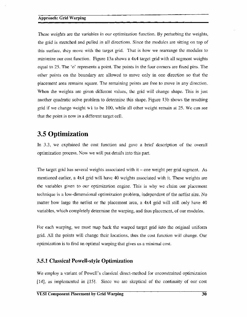
These weights are the variables in our optimization function. By perturbing the weights,

the grid is stretched and pulled in all directions. Since the modules are sitting on top of

this surface, they move with the target grid. That is how we rearrange the modules to

minimize our cost function. Figure 13a shows a 4x4 target grid with all segment weights

equal to 25. The ’o’ represents a point. The points in the four comers are fixed pins. The

other points on the boundary are allowed to move only in one direction so that the

placement area remains square. The remaining points are free to move in any direction.

When the weights are given different values, the grid will change shape. This is just

another quadratic solve problem to determine this shape. Figure 13b shows the resulting

grid if we change weight wl to be 100, while all other weight remain at 25. We can see

that the point is now in a different target cell.

3.5 Optimization

In 3.3, we explained the cost function and gave a brief description of the overall

optimization process. Now we will put details into this part.

The target grid has several weights associated with it - one weight per grid segment. As

mentioned earlier, a 4x4 grid will have 40 weights associated with it. These weights are

the variables given to our optimization engine. This is why we claim our placement

technique is a low-dimensional optimization problem, independent of the netlist size. No

matter how large the netlist or the placement area, a 4x4 grid will still only have 40

variables, which completely determine the warping, and thus placement, of our modules.

For each warping, we must map back the warped target grid into the original uniform

grid. All the points will change their locations, thus the cost function will change. Our

optimization is to find an optimal warping that gives us a minimal cost.

3.5.1 Classical Powe|l-style Optimization

We employ a variant of Powell’s classical direct-method for unconstrained optimization

[14], as implemented in [15]. Since we are skeptical of the continuity of our cost



function, but we need to minimize the number of evaluations of our expensive cost

function, we selected Powell as a reasonable starting choice for a direct method.

Powell is an algorithm that minimizes a given m dimensional cost function by

minimizing along specified direction vectors. So given a starting solution (a set of

weights in our case) and a direction vector, Powell calls a line minimization algorithm (to

be discussed momentarily), and when it returns, Powell has an improved m dimensional

solution. This process repeatedly continues, minimizing the cost function through all of

the m direction vectors until the relative decrease in the cost function is minimal.

The choice of direction vectors is key in minimizing the number of calls to the line

minimization algorithm, since we want to minimize in the direction that is most

beneficial. Simply put, we want to take a few large steps instead of several small ones.

Initially the direction vectors are unit vectors because we do not know, or wish to

calculate, gradients. During the execution of the algorithm these directions are selectively

replaced. It seems counterintuitive, but after each cycle through the direction vectors, the

direction providing the largest decrease is replaced by the average of all the directions.

The idea is that this direction will be a major component of the average; so replacing it

will reduce the linear dependencies of the set.

The line minimization algorithm used by Powell is called Brent’s method [14]. It is a

one-dimensional search trying to accelerate classical golden selection search using

inverse parabolic interpolation. The golden selection search is a well-known iterative

search algorithm that brackets a local minimum with three points. With each iteration it

closes in on the bracketed minimum until the window is sufficiently small (please refer to

Figure 15). Brent’s method attempts to find the minimum in only one iteration by finding

the minimum of a parabola that has been fitted to these three points. If the parabola is an

accurate model of the given cost function, then it has succeeded in finding the minimum

quickly; otherwise it resorts to the golden selection search algorithm.



Figure 15. One-dimension Search - This figure is from [14]. This search brackets a local

minimum with three points and repeats the process to find the local minimum.

3.5.2 Evaluation of the Cost Function

The cost function will need to be evaluated numerous times due to Powell’s repeated

calls to the line minimization algorithm. This means the target cells’ capacities and wire

lengths both need to be calculated. The calculations themselves are straightforward, but

we first must determine which point is in which target grid cells. For this Fowler used a

scan-line heuristic.

Scan-line algorithms have been widely used in the EDA community for mask checking. It

requires two tables: an edge table and an active edge table. In our case, each edge is a

target grid segment. The edge table is build using a bucket sort; where the number of

buckets corresponds to the number of scan lines. The number of scan lines, for us, is the

number of rows in the source grid. The edge table is sorted by each edge’s smaller y

coordinate, and within each bucket, sorted by each edge’s corresponding x coordinate.

The active edge table is initially empty. Then the edge table bucket with the smallest y

coordinates is moved into the active edge table and sorted by x coordinates. By simply

walking the active edge table, we are able to determine which x coordinates, and

therefore which source grid cells, correspond to which target grid cells, and we insert this

target gird cell number into a list of this source grid cell. Once a source grid cell is ending



or a new target grid segment is touched, the active edge table is updated. The next line

then is ready to be processed, so the edge table bucket with the next smallest y

coordinates is moved into the active edge table and re-sorted on x. This continues until

both tables are empty. (See figure 16 for an example)

Figure 16. Scan-line Algorithm - This is an example. Scan-line algorithm is run on each row.

For the row we choose in this figure, there are 8 possible target grid cells the point can belong to:

4 -ll, as indicated in the picture. For this 10xl0 source grid, we take out this row and run the

scan-line algorithm. We begin from the left most edge and walk from left to right, we only

consider the segments in this row’s range. After the scan-line algorithm, each source grid cell’s

list will be built up. For example, the 9th cell here finally get the list: 6->7->11->/. This means the

points in this cell can only belong to target grid cell 6, 7 or 11.

After the scan-line algorithm is done, each source grid cell has a list of target grid cell

numbers that the points in this source grid cell can only belong to one of these target grid

cells. Once we have this list, in the mapping back step, we need to determine which point

belongs to which target grid cell in the list. Then we can map this point back according to

the target grid cell’s location and we’re able to calculate each of the cost function

components once all the points are mapped back into their new locations. Here we use



bilinear mapping to map back the points. Bilinear mapping was introduced in 3.3 already.

Figure 17 shows an example of placement before and after bilinear mapping.

Figure 17. The placement before and after mapping - The left picture shows the warped grid

with all the points at their original locations. The right picture shows the grid is mapped back to a

uniform grid and all the points are mapped to their new locations.

3.5.3 Iterative Sequential Warping

Fowler’s original formulation for warping assumed a standard recursive decomposition in

which each cell in the warped placement is itself recursive warped. However, this is too

slow and we want to use a relatively quick way to try some experiments.

Notice the fact that one optimization can only find us one warping. So actually we do

three Powell steps, the latter one starts from the former one’s placement and begins to

find a new warping. We also use different target grid sizes here to add the flexibility. We

first use a coarse 2x2 target grid and use Powell to optimize, Then after this, we start our

2"a Powell step using a finer 3x3 target grid. Finally we use a yet finer 4x4 target grid and

run our final optimization step - the 3ra Powell step. After this step, we are done; we

currently do not use any recursion hierarchy, instead, we used this fast algorithm to try

some experiments. For large designs, of course we must recursively apply our algorithm



deep into each sub-region to further improve the layout. Our goal is this work was to re-

implement and tune Fowler’s initial warping kernel, and render it into form suitable to

use as the basis of ongoing experiments with warping.

We show the pseudo code of our algorithm below:

Grid-Warping Placement Algorithm:

1. Quadratic Placement Algorithm: Get the initial Quadratic Placement.

2. Build up the source grid so that each column and each row have the same number of

modules. Do Pre-Warping to spread out the dense clusters.

3. Begin our 1st Powell step

3.1 Starting from the given placement

3.2 Put a uniform grid on top of the chip

3.3 For each one-dimensional search

3.3.1 Perturb the segments’ weights, we call this vector x

3.3.2 Use another quadratic solve to get the warped grid’s location

3.3.3 Map every point into its new locations

3.3.4 Evaluate the cost function

3.3.5 Find the optimal solution in this dimension, update x

4. Go on with the 2nd and 3rd Powell steps

5. Final legalization step

Finish

3.6 Final Legalization

Our goal is not to take a very large net list all the way to legalization. We only want to

get close enough to drop it into a detailed placement polisher such as DOMINO.

Currently, we simply snap the final placement into rows by their y-coordinates before

putting it into DOMINO. One of our contributions in this work was implementing the

formulation for a more complete top-to-bottom flow from net-list, to rough placement, to

legalized row-based placement via the DOMINO tool. Fowler’s original warping kernel



lacked any backend integration with a real detailed legalization engine. Solving this was a

tedious but essential step for us, as it allows us now to compare our ongoing warping

results with a more standard placement flow, i.e., GORDIAN.

Before we are able to drop our placement into something like DOMINO, we believe a

few more steps may be necessary. Recall GORDIAN. To legalize their final placement of

standard cells, they only snapped the modules into rows, which proved to be very

inefficient. In contrast, PROUD made over half of their total wire length improvements in

their final legalization steps. These observations may imply we need to do something

similar.

Instead of only snapping the modules in rows, we may try PROUD’s technique of

looking at a small window, a target grid cell in our case, and apply a greedy algorithm to

improve the wire length. This may give us a better placement that will allow DOMINO,

or something similar, to finish the layout.

3.7 Summary

We reused Fowler’s original warping formulation, and described each of its steps. We

have completely re-implemented her initial warping kernel in a more modem object-

oriented style, integrated it in a standard placement flow, and introduced the idea of

replacing one single "deep" warping with a set of quicker coarse-to-fine sequential

warping. We describe our results in the following section.


4 Experimental Results

4.1 Experimental Methodology

We acquired 18 benchmarks from the ISPD98 circuit benchmark suite [ 16] ranging from

about 10,000 to 210,000 modules. These benchmarks, listed in Table 1, were converted to

our input format; however, there was no information on initial placement area, module

size, or I/O pad locations.

We noticed these benchmarks had recently been used by Cong, et al, in [17] [18] to

compare their new placer technique to that of GORDIANLfDOMINO. They did not

specify an initial placement area and their I/O pads were located in a single line on one

edge of the chip area, as opposed to around the placement boundary. As a result, we

added ten percent to the total module area, assuming, as [17] did, each module was one

hundred square units. I/O pads were randomly placed around the boundary at the 8

compass points.

We ran these modified benchmarks on our re-implemented and improved warping engine

and compared our resulting wire length and CPU times to that of GORDIANL. We also

ran our placement through DOMINO to get our final legal placement, and also ran

GORDIANL’s placement through DOMINO to get a comparison reference final

placement. We compare the final wire length to the wire length of

GORDIANL/DOMINO.


Experimental Results

The wire length of each net was computed as the half perimeter of the enclosing

bounding box. All CPU times are in seconds and are the overall running times.

# OF MODULES # OF NETS # OF ~O PADS # OF PINS

lbm01 12506 14111 246 50566

Ibm02 19342 19584 259 81199

Ibm03 22853 27401 283 93573

Ibm04 27220 31970 287 105859

Ibm05 28146 28446 1201 126308

Ibm06 32332 34826 166 128182

Ibm07 45639 48117 287 175639

Ibm08 51023 50513 286 204890

Ibm09 53110 60902 285 222088

Ibml0 68685 75196 744 297567

Ibmll 70152 81454 406 280786

Ibml2 70439 77240 637 317760

Ibm13 83709 99666 490 357075

Ibm14 147088 152772 517 546816

Ibml5 161187 186608 383 715823

Ibm16 182980 190048 504 778823

Ibml7 184752 189581 743 860036

lbml8 210341 201920 272 819697

Table 1: Benchmarks

4.2 Results and Analysis

All benchmarks were run with a 20x20 source grid. All benchmarks were run with three

Powell steps with the 2x2, 3x3, and 4x4 target grids respectively. Our placement



algorithm was run on a SUN Solaris CPU with 750MHz, GORDIANL and DOMINO

were run on a Linux machine with a single 750MHz CPU. It is fair, since we lack in our

current re-implementation of the warping engine any recursive placement step (as Fowler

originally had), we know a priori that our placement results will be inferior since they are

incomplete. Hence, we chose to run the GORDIAN flow at its "fast" setting, allows it to

trade wire length for run time. This is an imperfect, but not unreasonable comparison. We

do note here, however, that running GORDIAN at higher levels of effort can reduce wire

length by an additional 20-30%. For our placement algorithm, in the cost function, we set

the weight K equal to 1.

We compared our algorithm + DOMINO with GORDIANL + DOMINO. Table 2 shows

the resulting wire length and CPU times of both methods. We give raw wire length and

CPU time for GORDIANL+DOMINO, and for our own placer, give normalized relative

wire length and CPU time by dividing our results by GORDIANL + DOMINO’s results.

For CPU times, values larger than 1.0 mean that GORDIANL + DOMINO’s approach is

better or faster, while values smaller than 1.0 would mean that our approach is better or

faster. For wire length, values larger than 1.0 mean that GORDIANL + DOMINO’s

approach is better, while values smaller than 1.0 mean that our approach is better.

GORDIANL + DOMINO

WIRE LENGTH CPU TIIVIE

OUR PLACER + DOMINO

WIRE LENGTH CPU TIME

Ibm01 1.68e6 175.8 1.14 1.20

Ibm02 4.59e6 533.9 NA NA

Ibm03 5.99e6 508.0 1.01 0.77

Ibm04 6.79e6 521.9 1.14 1.23

Ibm05 1.17e7

Ibm06 8.28e6

lbm07

1045.0 1.03 0.74

1001.5 1.02 0.95

1082.2

2420.4lbm08

1.07e7 1.25

1.261.15e7

1.92

0.56

Ibm09 1.20e7 1389.1 1.19 1.02



Ibm 10 1.96e7 2227.8 1.20 0.98

Ibml 1 2.20e7 1881.0 0.95 0.97

Ibml2 2.96e7 2359.3 0.97 0.99

Ibm13 2.50e7 2809.5 1.12 0.97

Ibm14 4.53e7 6237.7 1.24 0.74

Ibml5 6.84e7 8529.2 1.06 0.67

Ibm16 5.54e7 9611.4 1.41 0.84

Ibml7 8.91e7 10798.3 1.05 0.62

Ibml8 7.90e7 14274.9 1.06 0.48

Table 2: Comparison between our approach and GORDIANL + DOMINO

From the results we can see that our wire length is as expected, inferior to GORDIANL +

DOMINO’s, but on average we are only 10% worse. However, we are faster, our speed

increases as the net-list sizes increase.

Of course, again, the comparison is imperfect. Our warping engine is as incomplete, and

is a partial attempt to "level" the comparison; we ran the GORDIAN flow at its faster,

lower quality setting. Nevertheless, we are pleased with these intermediate results, and

note that Fowler’s original engine, which lacked our integration with DONIMO, but did

have a full recursion capability, was producing wire lengths closer to 50% over the

GORDIAN result. We believe we are headed in the right direction. And the reasons why

our wire length is not as good as it could be:

1) No linear re-weighting: The GORDIANL work suggests that a linear re-

weighting scheme saves 20-30% on total wire length. We are not implementing

any re-weighting. Perhaps part of our wire length penalty relative to GORDIAN

is from this alone.

2) Compromised mobility of clusters: Our initial attempts at pre-warping, following

Fowler’s strategy, were intended to spread out the clusters by roughly one order

of magnitude. We succeeded in doing this, but it seems that the very small dense

clusters were not fully weighted in our equation. We were unable to break them

apart and relocate their individual modules to the appropriate locations. We



3)

believe that we need a more sophisticated non-uniform pre-warping. An adaptive

mesh, in the style of 2D finite elements, seems the right direction here.

Optimization Engine: We selected a classical Powell downhill optimizer because

of its ease of implementation, and the fact that it required no derivatives. Powell

works quite well for us, but the number of calls to our cost function determines

our mntime, which is a large flat evaluation of layout quality. We are considering

revisiting our "no derivatives" assumption: we need to see empirically how

smooth the space of grid edge weights really is. If it is reasonably smooth, a more

modem trust region method, e.g. [19], might give us a significant reduction in

runtime.

We note here finally that the differences in run-times among the experiments make sense.

As mentioned before, this algorithm is low dimensional and inherently parallel. Not only

could each target grid cell be optimized in parallel, but also the cost function could be

split into sections and calculated in parallel. We believe this would greatly reduce the

run-times since these optimizations and calculations are fairly data independent.

It is important to point out that as the size of the net-lists increase, the ratio between our

CPU times and GORDIANL’s increases. This implies that as the placement problem

grows, our algorithm has the potential of handling this size, whereas GORDIANL begins

to slow down.

4.3 Summary

We re-implemented and enlarged Fowler’s original warping kernel, integrated it in a

GORDIAN-DOMINO flow, and experimented with the standard ISPD98 benchmark set.

At this point, we have re-implemented roughly 80% of the original engine; our current

engine has roughly 10,000 lines of C++.

We presented results from the ISPD98 benchmarks, ranging from about 10,000 to

210,000 modules. As expected, our placement quality is inferior, but demonstrate a range



of performance we regard as quite promising. Our very incomplete engine averages 10%

more wire length, but shows an accelerating speed up over the GORDIAN flow as

problem size increases.

An example placement of our algorithm:

Initial Quadratic Placement

After Pre-Warping, try to find an optimal 2x2 target grid, and warp the grid, change the

layout. This is done in the 1st Powell step.



Do the 2nd Powell step, using 3x3 target grid

Do the 3rd Powell step, using 4x4 target grid. It’s the final step and the final layout.


5 Conclusions

5.1 Summary

We believe the current placement algorithms will begin to break down as net-lists

continue to grow to 10-100 million gates. We described our efforts to re-implement and

enhance Fowler’s initial formulation of the grid-warping concept, to create a new

placement algorithm targeting these very large net-lists. The formulation of the problem

is essentially a low-dimensional optimization problem, independent of net-list size,

because we only optimize the target grid segment weights. This new technique is also

inherently parallel. These characteristics should allow us to handle these ever-increasing

net-lists, potentially better than existing tools.

We described an implemented completely new warping engine, and integrated it into a

GORDIAN-DOMINO flow for comparison. Preliminary results show much promise.

With additional research, we hope this technique can compete with current algorithms

and handle the net-lists of tomorrow.

5.2 Direction

The techniques and results presented here are preliminary and encourage further research

to refine this algorithm. Some future areas in our research will include:

1. Completing the missing recursion steps missing in our current version of the

warping engine


Conclusions

2. Try alternative cost function and nonlinear optimization formulations to improve

the results

3. Modifying the algorithm so that large computations are done in parallel

4. Accounting for module size so that they are no longer modeled as points.

We believe that our initial placer results show promise, and with further direction could

be on the right path to a very fast, efficient, and fiat algorithm that is able to quickly

handle large net-lists.


Bibliography

[1] R.S. Tsay, E. Kuh, C.P Hsu. "PROUD: A Sea-Of-Gates PlacementAlgorithm," IEEE Design & Test of Computers, December 1988.

[2] J. Kleinhans, G. Siegl, F.M. Johannes, K. Antreich. "GORDIAN:VLSI Placement by Quadratic Programming and SlicingOptimization," IEEE Transactions on Computer Aided Design,Vol. 10 No. 3, March 1991.

[3] G. Siegl, K. Doll, F.M. Johannes. "Analytical Placement: A Linearor a Quadratic Objective Function?" Proc. 28th Design AutomationConference, June 1991.

[4] C. J. Alpert, T. Chan, D. J.-H. Huang, I. Markov and K. Yan."Quadratic Placement Revisited" Proc. 34th Design AutomationConference, June 1997.

[5] J.R. Shewchuk. "An Introduction to the Conjugate GradientMethod Without Agonizing Pain", Carnegie Mellon University,August 1994.

[6] Gene H. Golub, Charles F. Van Loan. Matrix Computations, thirdedition, The Johns Hopkins University Press, 1996.

[7] K. Doll, F.M. Johannes, K.J. Antreich. "Accurate net models forplacement improvement by network flow methods," Proc. IEEEInt. Conf Computer Aided Design, 1992.


[8] K. Doll, F.M. Johannes, K.J. Antreich. "Iterative PlacementImprovement by Network Flow Methods," IEEE Transactions onComputer Aided Design, Vol. 13 No. 10,.October 1994.

[91 H. Eisenmann, F.M. Johannes. "Generic Global Placement andFloorplanning," Proc. Design Automation Conference, 1998.

[10] J. Vygen. "Algorithms for Large-Scale Flat Placement," Proc. 34th

Design Automation Conference, June 1997.

[11] C.K. Cheng, E.S. Kuh. "Module Placement Based on ResistiveNetwork Optimization," IEEE Transactions on Computer AidedDesign, Vol. 3, July 1984, pp. 218-225.

[12] P.S. Heckbert. "Fundamentals of Texture Mapping and ImageWarping," Master’s Thesis, University of California, Berkeley,June 1989.

[13] J.D. Foley, A. van Dam, S.K. Feiner, J.F. Hughes. ComputerGraphics, Principles and Practice. New York: Addison-WesleyPublishing Company, 1990.

[14] W.H. Press, et al. Numerical Recipes in C: The Art of ScientificComputing. New York: Cambridge University Press, 1992.

[15] M.J. Krasnicki. "A Methodology for Distributed Simulation-BasedSynthesis of Custom Analog Circuits", PhD Dissertation, CarnegieMellon University, December 2000.

[16] http://vldicad.cs.ucla.edu/-cheese/ispd98.html

[17] T.F. Chan, J. Cong, T. Kong, J.R. Shinner. "MultilevelOptimization for Large-Scale Circuit Placement," Proc.International Conference on Computer-Aided Design, 2000.

Placement by (~rid Warping 47

[18] Chin-Chih Chang, Jason Cong, Zhigang Pan, Xin Yuan "PhysicalHierarchy Generation with Routing Congestion Control," ISPD’02,April 7-10, 2002, San Diego, California, USA.

[19] A.R. Conn, N.I.M. Gould, Ph. Toint. "Trust-region methods,"MPS-SIAM Series on Optimization, SIAM Publications,Philadelphia, PA, USA, 2000.

[20] Suzanne M. Fowler "Placement by Grid Warping" MS thesis,Electrical and Computer Engineering Department, CarnegieMellon University, December 2001

Placement by Grid Warping 48

electrical & computer engineering & computer engineering. ... which are the bottleneck in...

Documents