electric vehicle used for commuting
TRANSCRIPT

energies
Article
Annual Variation in Energy Consumption of anElectric Vehicle Used for Commuting
Anatole Desreveaux 1,2, Alain Bouscayrol 1,2,*, Elodie Castex 3 , Rochdi Trigui 2,4 ,Eric Hittinger 1,5 and Gabriel-Mihai Sirbu 2,6
1 Department of Electronics, Electrical Engineering and Automation, Faculty of Sciences and Technology,University of Lille, Arts et Metiers Institute of Technology, Centrale Lille, Yncrea Hauts-de-France,ULR 2697–L2EP, F-59000 Lille, France; [email protected] (A.D.);[email protected] (E.H.)
2 French Network on HEVs and EVs, MEGEVH, 59650 Villeneuve D’Ascq, France;[email protected] (R.T.); [email protected] (G.-M.S.)
3 Univ. Lille, ULR 4477—TVES—Territoires Villes Environnement & Société, F-59000 Lille, France;[email protected]
4 AME-Eco7, Univ Gustave Eiffel, IFSTTAR, Univ Lyon, F-69675 Lyon, France5 Rochester Institute of Technology, Rochester, NY 14623, USA6 Renault Technologie Roumanie SRL, 062204 Bucharest, Romania* Correspondence: [email protected]
Received: 3 August 2020; Accepted: 1 September 2020; Published: 7 September 2020
Abstract: The energy consumption of an electric vehicle is primarily due to the traction subsystemand the comfort subsystem. For a regular trip, the traction energy can be relatively constant butthe comfort energy has variation depending on seasonal temperatures. In order to plan the annualcharging operation of an eco-campus, a simulation tool is developed for an accurate determination ofthe consumption of an electric vehicle throughout year. The developed model has been validatedby comparison with experimental measurement of a real vehicle on a real driving cycle. Differentcommuting trips are analyzed over a complete year. For the considered city in France (Lille), the comfortenergy consumption has an overconsumption up to 33% in winter due to heating, and only 15% insummer due to air conditioning. The urban commuting driving cycle is more affected by the comfortsubsystem than extra-urban trips.
Keywords: electric vehicle; energy consumption; traction; heating ventilation air conditioning;simulation; energetic macroscopic representation
1. Introduction
Climate change is a critical challenge for humanity in the 21st century. In developed countries,the transport sector is the largest producer of greenhouse gases that cause climate change. Electrificationof vehicles is a way to reduce pollutants emissions [1,2]. In fact, according to the International EnergyAgency, limiting climate change to 2 C is possible if 150 million electrified vehicles are on the roadby 2030 [3]. Many cities want to replace conventional vehicles by electrified vehicles or ban thermalvehicles completely [4].
As an example, the University of Lille would convert its “Cité Scientifique” into an eco-campuswithout thermal vehicles [5]. As this campus receives 22,000 daily users in 80 buildings, it is functionallya small city. Currently, mobility constitutes more than 50% of the greenhouse gas emissions of thiscampus. The CUMIN (Campus of University with Mobility based on Innovation and carbon Neutral)program [5] aims to reduce the emissions from thermal cars, using several strategies includingreplacing conventional vehicles with electric vehicles supplied by photovoltaic-based charging stations.
Energies 2020, 13, 4639; doi:10.3390/en13184639 www.mdpi.com/journal/energies

Energies 2020, 13, 4639 2 of 15
In anticipation of this shift, a simulation tool is necessary for calculating the amount of energy neededby the electric vehicles. This tool will be used to plan the required charging stations and photovoltaicpanels necessary to charge the vehicles from a defined electrification scenario.
However, EV adoption by commuters is only slowly increasing [3]. Charging infrastructure,charging time [6,7] and purchasing price [8] are important barriers to an increase of EV market share.Driving range is an important problem for EV adoption [7–9] even though charging infrastructureavailability and charging time remain other important issues. Range anxiety due to the high variationin driving range estimators within vehicles creates uncertainty about the range of the electric car [10].Consequently, accurate tools are necessary to estimate the driving range before and during a trip [11,12].
The driving range is related to the vehicle energy consumption and the battery behavior (storagecapacity). The energy consumption is mainly related to the vehicle traction, but also to the HVAC toheat or refresh the cabin. A large number of studies present different factors that impact this energyconsumption. The weather and climatic conditions can have an important impact on the energyconsumption of the traction subsystem [13] and the Heating, Ventilation, Air Conditioning (HVAC)consumption [14–17]. Battery capacity decreases and battery losses increase when the temperaturefalls below 0 C [17–19]. Moreover, traffic conditions [20–23] such as velocity limitations, accelerations,traffic jams and traffic stops also have an important impact. Furthermore, driver behavior [21–24]impacts the energy consumption of the vehicle.
However, most EV simulation tools do not consider all of these factors at the same time to assessthe global energy consumption of the vehicle [12]. Generally, studies are limited to a small number offactors that are easier to calculate. For example, the combined effect of the road trip and temperatureare generally not studied at the same time.
Different methodologies exist to estimate the energy consumption of vehicles. One group ofmethods is based on real-world measurements [25,26]. These tools aggregate a large quantity ofhistorical data from different vehicles and can give a good estimation of energy consumption inthe future. However, this type of tool is difficult to adapt to new vehicles without a lot of timeand investment into data measurement. Another group of methods is based on physical vehiclemodeling [27]. These methods are generally used for energy consumption calculations [13,22],routing problems [28] and energy management strategies [29,30]. They also depend on the parametersof the vehicle and are more flexible in application. In this article, a vehicle model is developed for usein a flexible simulation tool. This model allows for decoupling of the effects between the HVAC andthe traction subsystems.
In [22] an accurate traction model of an EV has been developed to study the impact of velocityprofiles on energy consumption, independently of the other factors (such as the climate, driver behaviorsor traffic). In this paper, the comfort subsystem of the vehicle is added to the previously developedvehicle model. The objective of this paper is to study the annual variation of the energy consumptionof an electric vehicle used for commuting trips. The method seeks to include the supplementaryconsumption due to the HVAC independently of the other factors (such as the traffic, driver behavior,or battery behavior), so that it can be isolated and compared to those other factors. A simulationpackage is developed to compute the energy for the traction and HVAC subsystems. The supplementaryenergy due to heating or air conditioning can thus be estimated throughout the year under changingclimate conditions.
Section 2 develops the simulation tool of the vehicle. This tool is then validated with measurementson an actual electric vehicle. Section 3 deals with annual variation in energy consumption for an urbantrip. Then, the annual variation is extended to different daily trips in Section 4. The accuracy andcomparison of the effect of different factors are also discussed in this section.

Energies 2020, 13, 4639 3 of 15
2. Simulation Tool for an Electric Vehicle
2.1. Modeling of the Electric Vehicle
The chosen EV for the simulation tool is the Renault Zoé (Figure 1) [31]. The main parametersof the vehicle are given in Table 1. This case study is applied to a moderate oceanic climate and thethermal effect of the battery is not considered. While including thermal effects on the battery is relevant,prior research suggests that battery capacity is mainly impacted for temperatures below 0 C [18].Future work that applies this model to other climates will require a more complex battery model.The driver is modeled by a simple proportional integral controller. Thus, this work does not varydriver behavior and focuses only on the effects of climate and commuting route.
Energies 2020, 13, x FOR PEER REVIEW 3 of 15
2. Simulation Tool for an Electric Vehicle
2.1. Modeling of the Electric Vehicle
The chosen EV for the simulation tool is the Renault Zoé (Figure 1) [31]. The main parameters of
the vehicle are given in Table 1. This case study is applied to a moderate oceanic climate and the thermal
effect of the battery is not considered. While including thermal effects on the battery is relevant, prior
research suggests that battery capacity is mainly impacted for temperatures below 0 °C [18]. Future
work that applies this model to other climates will require a more complex battery model. The driver
is modeled by a simple proportional integral controller. Thus, this work does not vary driver behavior
and focuses only on the effects of climate and commuting route.
Figure 1. The studied Renault Zoé before the validation test.
Table 1. Parameters of the studied Electric Vehicle.
Elements Characteristics
Battery Li–ion NMC–22 kWh
Electric Machine Synchronous machine 65 kW
Weight 1468 kg
2.1.1. Modeling of the Traction and Battery Subsystems
The traction subsystem of the electric vehicle is composed of an electric drive, a gearbox, the
wheels and a chassis. The modeling of the traction subsystem has been developed in [22].
The battery voltage ubat depends on the open-circuit voltage (OCV) uocv, the current ibat and the
battery resistance Rbat. The OCV depends on the State-of-Charge (SoC) of the battery.
𝑢𝑏𝑎𝑡 = 𝑢𝑜𝑐𝑣(𝑆𝑜𝐶) + 𝑅𝑏𝑎𝑡𝑖𝑏𝑎𝑡 (1)
The battery is connected to the auxiliaries, the HVAC subsystem, and the electric drive. The
battery current ibat is the sum of the electric drive currents, the auxiliary current iaux and the HVAC
current iHVAC.
𝑖𝑏𝑎𝑡 = 𝑖𝑒𝑑 + 𝑖𝑎𝑢𝑥 + 𝑖𝐻𝑉𝐴𝐶 (2)
The torque of the electric drive Γed depends on the reference torque Γed_ref. The current of the
electric drive depends on the electric drive torque Γed, the speed of the gearbox Ωgb, the battery voltage
ubat and a static efficiency ηed = 87%. For the expected accuracy of range estimation, prior research
suggests that a static model for the electric drive is sufficient for calculation of the traction energy
consumption [32].
𝛤𝑒𝑑 = 𝛤𝑒𝑑_𝑟𝑒𝑓
𝑖𝑒𝑑 = 𝛤𝑒𝑑𝛺𝑔𝑏𝜂𝑒𝑑
𝑘𝑒𝑑
𝑢𝑏𝑎𝑡
with 𝑘𝑒𝑑 = −1 if 𝛤𝑒𝑑𝛺𝑔𝑏 < 0
1 if 𝛤𝑒𝑑𝛺𝑔𝑏 ≥ 0 (3)
The gearbox speed Ωgb depends on the wheel speed Ωwh and the gearbox ratio kgb. The gearbox
torque Γgb depends on the electric drive torque Γed, the gearbox ratio and the gearbox efficiency ηgb.
Figure 1. The studied Renault Zoé before the validation test.
Table 1. Parameters of the studied Electric Vehicle.
Elements Characteristics
Battery Li–ion NMC–22 kWhElectric Machine Synchronous machine 65 kW
Weight 1468 kg
2.1.1. Modeling of the Traction and Battery Subsystems
The traction subsystem of the electric vehicle is composed of an electric drive, a gearbox, the wheelsand a chassis. The modeling of the traction subsystem has been developed in [22].
The battery voltage ubat depends on the open-circuit voltage (OCV) uocv, the current ibat and thebattery resistance Rbat. The OCV depends on the State-of-Charge (SoC) of the battery.
ubat = uocv(SoC) + Rbatibat (1)
The battery is connected to the auxiliaries, the HVAC subsystem, and the electric drive. The batterycurrent ibat is the sum of the electric drive currents, the auxiliary current iaux and the HVAC current iHVAC.
ibat = ied + iaux + iHVAC (2)
The torque of the electric drive Γed depends on the reference torque Γed_ref. The current of theelectric drive depends on the electric drive torque Γed, the speed of the gearboxΩgb, the battery voltageubat and a static efficiency ηed = 87%. For the expected accuracy of range estimation, prior researchsuggests that a static model for the electric drive is sufficient for calculation of the traction energyconsumption [32].
Γed = Γed_re f
ied =ΓedΩgbη
keded
ubat
with ked =
−1 if ΓedΩgb < 01 if ΓedΩgb ≥ 0
(3)
The gearbox speed Ωgb depends on the wheel speed Ωwh and the gearbox ratio kgb. The gearboxtorque Γgb depends on the electric drive torque Γed, the gearbox ratio and the gearbox efficiency ηgb.
Energies 2020, 13, 4639 4 of 15
Ωgb = Ωwhkgb
Γgb = Γedkgbηkg
gbwith ked =
−1 i f ΓedΩgb < 01 i f ΓedΩgb ≥ 0
(4)
The wheel transforms the vehicle velocity vev into wheel speed Ωwh with the wheel radius Rwhand the gearbox torque Γgb into the wheel force Fwh. Ωwh = vev
Rwh
Fwh =ΓgbRwh
(5)
The wheel force Fwh is added to the mechanical braking force Fbr to give the total force applied tothe vehicle Ftot.
Ftot = Fwh + Fbr (6)
Newton’s second law is used to calculate the velocity of the car vev, which depends on the totaltraction force, resistive force to the motion Fres and the vehicle mass Mev.
vev =1
Mev
∫(Ftot − Fres)dt (7)
The resistive force Fres is composed of the aerodynamic force Fa, the road resistance force Fr andthe slope Fs.
Fres = Fa + Fr + Fs (8)
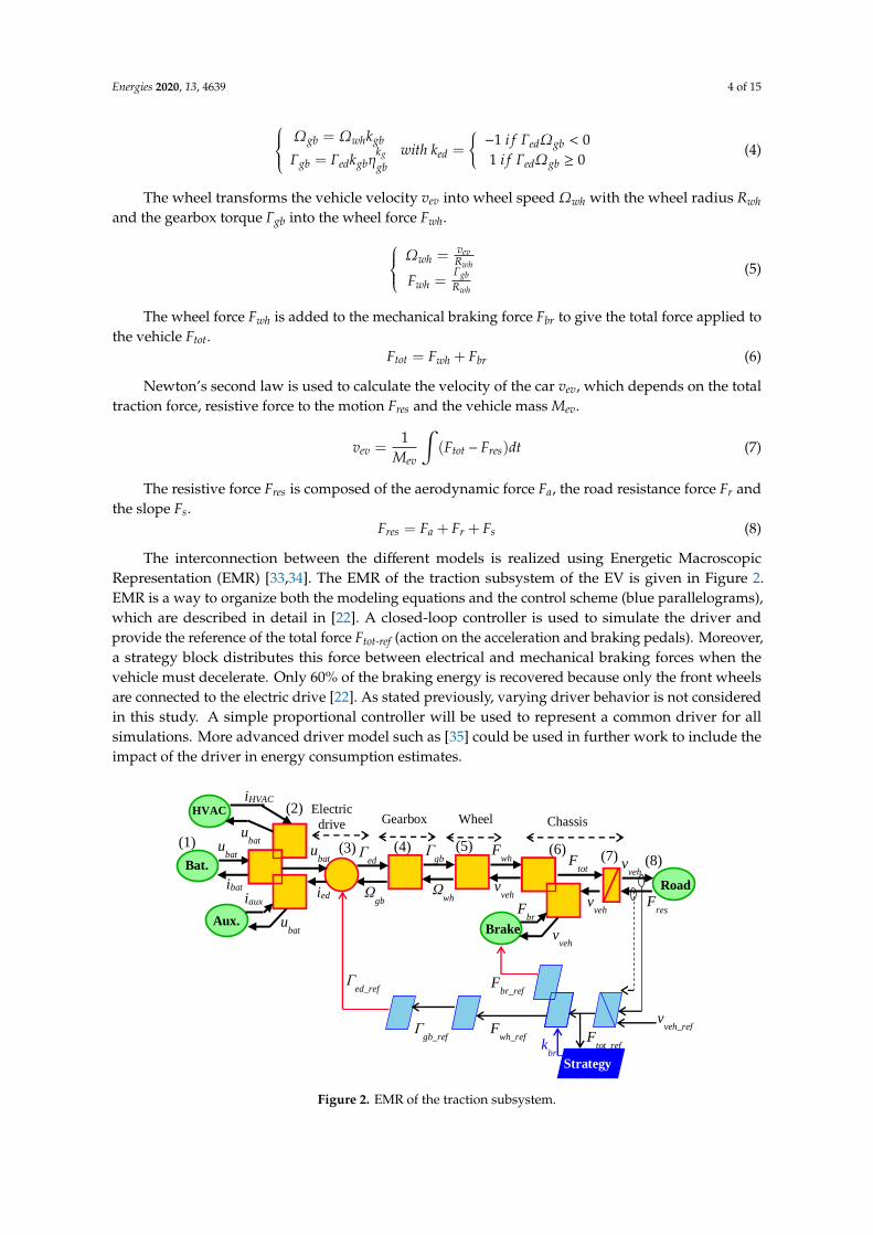
The interconnection between the different models is realized using Energetic MacroscopicRepresentation (EMR) [33,34]. The EMR of the traction subsystem of the EV is given in Figure 2.EMR is a way to organize both the modeling equations and the control scheme (blue parallelograms),which are described in detail in [22]. A closed-loop controller is used to simulate the driver andprovide the reference of the total force Ftot-ref (action on the acceleration and braking pedals). Moreover,a strategy block distributes this force between electrical and mechanical braking forces when thevehicle must decelerate. Only 60% of the braking energy is recovered because only the front wheelsare connected to the electric drive [22]. As stated previously, varying driver behavior is not consideredin this study. A simple proportional controller will be used to represent a common driver for allsimulations. More advanced driver model such as [35] could be used in further work to include theimpact of the driver in energy consumption estimates.
Energies 2020, 13, x FOR PEER REVIEW 4 of 15
𝛺𝑔𝑏 = 𝛺𝑤ℎ𝑘𝑔𝑏
𝛤𝑔𝑏 = 𝛤𝑒𝑑𝑘𝑔𝑏𝜂𝑔𝑏𝑘𝑔 with 𝑘𝑒𝑑 =
−1 𝑖𝑓 𝛤𝑒𝑑𝛺𝑔𝑏 < 0
1 𝑖𝑓 𝛤𝑒𝑑𝛺𝑔𝑏 ≥ 0 (4)
The wheel transforms the vehicle velocity vev into wheel speed Ωwh with the wheel radius Rwh
and the gearbox torque Γgb into the wheel force Fwh.
𝛺𝑤ℎ =
𝑣𝑒𝑣
𝑅𝑤ℎ
𝐹𝑤ℎ = 𝛤𝑔𝑏
𝑅𝑤ℎ
(5)
The wheel force Fwh is added to the mechanical braking force Fbr to give the total force applied to
the vehicle Ftot.
𝐹𝑡𝑜𝑡 = 𝐹𝑤ℎ + 𝐹𝑏𝑟 (6)
Newton’s second law is used to calculate the velocity of the car vev, which depends on the total
traction force, resistive force to the motion Fres and the vehicle mass Mev.
𝑣𝑒𝑣 = 1
𝑀𝑒𝑣∫(𝐹𝑡𝑜𝑡 − 𝐹𝑟𝑒𝑠)𝑑𝑡 (7)
The resistive force Fres is composed of the aerodynamic force Fa, the road resistance force Fr and
the slope Fs.
𝐹𝑟𝑒𝑠 = 𝐹𝑎 + 𝐹𝑟 + 𝐹𝑠 (8)
The interconnection between the different models is realized using Energetic Macroscopic
Representation (EMR) [33,34]. The EMR of the traction subsystem of the EV is given in Figure 2. EMR
is a way to organize both the modeling equations and the control scheme (blue parallelograms),
which are described in detail in [22]. A closed-loop controller is used to simulate the driver and
provide the reference of the total force Ftot-ref (action on the acceleration and braking pedals).
Moreover, a strategy block distributes this force between electrical and mechanical braking forces
when the vehicle must decelerate. Only 60% of the braking energy is recovered because only the front
wheels are connected to the electric drive [22]. As stated previously, varying driver behavior is not
considered in this study. A simple proportional controller will be used to represent a common driver
for all simulations. More advanced driver model such as [35] could be used in further work to include
the impact of the driver in energy consumption estimates.
Bat.
Brake
Road
Chassis Wheel Gearbox
Strategy
Γgb_ref
Γgb
ubat
Fwh
Fres
F
br
vveh
vveh
vveh
v
veh
vveh_ref
Fbr_ref
Fwh_ref
F
tot_ref
ibat Ωwh
kbr
Ftot
Aux.
Electric drive
ubat
ubat
ied iaux
Γed
Ωgb
Γed_ref
ubat
iHVAC HVAC
(1)
(2)
(3) (4) (5) (6) (7) (8)
Figure 2. EMR of the traction subsystem.
Figure 2. EMR of the traction subsystem.
Energies 2020, 13, 4639 5 of 15
2.1.2. Modeling of the Comfort Subsystem
The comfort subsystem is composed of a heat pump, a heater, a fan (HVAC) and the cabin’sthermal behavior. The HVAC subsystem modeling adapts the heating model developed in [36] foranother electric vehicle but adds air conditioning and ventilation elements.
The heat pump is composed of an electric compressor, two heat exchangers and an expansionvalve. The electric machine of the compressor is modeled with a static model where the rotation speedΩcomp is imposed by the controller, and the current ihp depends on the mechanical power, the batteryvoltage and the machine efficiency ηcom. Ωcomp = Ωcomp_re f
ihp =Γcomp Ωcomp ηcomp
ubat
(9)
Two equivalent volumetric flows of the refrigerant, one for each exchanger (qve1, qve2) and themachine torque Γcomp can be calculated as a function of the compressor speedΩcomp, the two exchangerpressures pe1 and pe2, the two refrigerant enthalpies he1 and he2 and the mass flow of the refrigerantqmcomp. The equations of the last three variables are given in [36].
Γcomp =qmcomp(he2−he1)
Ωcomp
qve1 =qmcomphe1
pe1
qve2 =qmcomp he2
pe2
(10)
For the two heat exchangers, three equations are necessary to describe their behavior. The firstequation gives the accumulation of pressure inside the exchanger. The pressure on the exchanger pe
depends on the initial pressure pinit, the volume of the refrigerant inside the exchanger Ve, and twovolumetric flows (qva and qvb,), which depend on the heat exchanger inputs (see the EMR of the heatpump). Ke is a parametric function which depends on the heat exchanger pressure. More details onthis function are given in [36].
pe = pinit exp(
1Ve
∫ ( 1Ke
(qva − qvb)dt))
(11)
The heat exchanger exchanges heat between the refrigerant and the heat exchanger wall.The refrigerant loses heat with this exchange. The volumetric flow qvb is a function of the volumetricflows qvc and qvd. It can be calculated as a function of the exchanger heat flow qse, the exchangerpressure pe and the exchanger temperature Te which depends on the temperature of the refrigerant atthe considered pressure T(pe).
qvb = qvc − qvdTe = T(pe)
qvd =Teqse
pe
(12)
The volumetric flows qva and qvc depend on the volumetric flow of the expansion valve and thecompressor (see the EMR of the heat pump in Figure 3). Convection drives the exchange betweenthe air and the heat exchanger. The heat flows qse and qse_out are a function of the temperature of theexchanger Te, the temperature of the air outside the exchanger Te_out and the convection coefficient Kairwhich depends on additional parameters. More details on this coefficient are given in [16]. qse = Kair
(Te−Te_out)Te_out
qse_out = Kair(Te−Te_out)
Te
(13)
Energies 2020, 13, 4639 6 of 15Energies 2020, 13, x FOR PEER REVIEW 6 of 15
DC bus
Cab.
Air
qshp
qse1
pe2
Te1
Tcab
qve4
qve1
qse2
qsair_e2
T
e2
Tamb
ihp
ubat
Ωcomp
Γcomp
Ωcomp_ref
pe1
pe2
qve2
qve3
pe2
pe1
pe1
qve_tot1
qve_tot2
qmcomp
Ωcomp_ref
pe1_ref
Te1_ref
qshp_ref
qv
e2_ref
qve1_mes
p
e1_mes
Tcab_mes
qv
e1_tot_mes
(14)
(13)
(13)
(11)
(11)
(10)
(12)
(12)
(9)
Compressor
Heat exchanger 1
Heat exchanger 2
Expansion valve
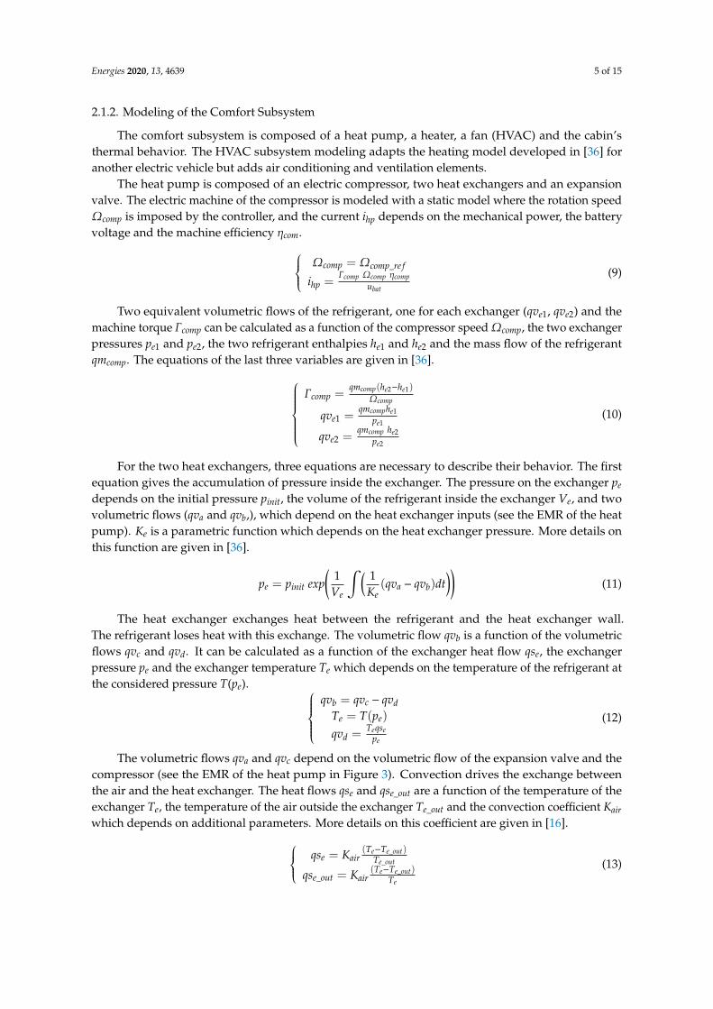
Figure 3. EMR of the heat pump.
The expansion valve gives two volumetric flows qve3 and qve4 as a function of the pressure on the
two heat exchangers pe1 and pe2, the mass flow of the refrigerant qmcomp and the enthalpy flows he3 and
he4. The equations for the enthalpy flows are given in [36].
𝑞𝑣𝑒4 =
𝑞𝑚𝑐𝑜𝑚𝑝ℎ𝑒4𝑝𝑒1
𝑞𝑣𝑒3 =𝑞𝑚𝑐𝑜𝑚𝑝ℎ𝑒3
𝑝𝑒2
(14)
The EMR of the heat pump is given in Figure 3. The control is deduced from the previous
equations by inversion: closed-loop control for accumulation elements (crossed rectangles) and direct
inversion for other elements [33].
The cabin thermal behavior is modeled following the equations given in [16]. The comfort model
is organized using EMR (Figure 4).
Figure 3. EMR of the heat pump.
The expansion valve gives two volumetric flows qve3 and qve4 as a function of the pressure on thetwo heat exchangers pe1 and pe2, the mass flow of the refrigerant qmcomp and the enthalpy flows he3 andhe4. The equations for the enthalpy flows are given in [36]. qve4 =
qmcomphe4pe1
qve3 =qmcomphe3
pe2
(14)
The EMR of the heat pump is given in Figure 3. The control is deduced from the previous equationsby inversion: closed-loop control for accumulation elements (crossed rectangles) and direct inversionfor other elements [33].
The cabin thermal behavior is modeled following the equations given in [16]. The comfort modelis organized using EMR (Figure 4).
2.2. Validation of the EV Simulation Tool
The traction subsystem has been validated in [22]. The current work validates the global vehiclemodel (combining the traction and comfort subsystems), realized with a driving test that also uses airconditioning. The vehicle is driven on an urban trip of 40 min duration (Figure 5). The trip length is14 km.

Energies 2020, 13, 4639 7 of 15Energies 2020, 13, x FOR PEER REVIEW 7 of 15
Figure 4. EMR of the comfort subsystem.
2.2. Validation of the EV Simulation Tool
The traction subsystem has been validated in [22]. The current work validates the global vehicle
model (combining the traction and comfort subsystems), realized with a driving test that also uses
air conditioning. The vehicle is driven on an urban trip of 40 min duration (Figure 5). The trip length
is 14 km.
Figure 5. Urban driving cycle measured with the vehicle.
The ambient temperature was 24 °C during this trip. During the test, the cabin temperature was
maintained at 19 °C (Figure 6), despite the ambient temperature, thanks to the HVAC subsystem.
Figure 4. EMR of the comfort subsystem.
Energies 2020, 13, x FOR PEER REVIEW 7 of 15
Figure 4. EMR of the comfort subsystem.
2.2. Validation of the EV Simulation Tool
The traction subsystem has been validated in [22]. The current work validates the global vehicle
model (combining the traction and comfort subsystems), realized with a driving test that also uses
air conditioning. The vehicle is driven on an urban trip of 40 min duration (Figure 5). The trip length
is 14 km.
Figure 5. Urban driving cycle measured with the vehicle.
The ambient temperature was 24 °C during this trip. During the test, the cabin temperature was
maintained at 19 °C (Figure 6), despite the ambient temperature, thanks to the HVAC subsystem.
Figure 5. Urban driving cycle measured with the vehicle.
The ambient temperature was 24 C during this trip. During the test, the cabin temperature wasmaintained at 19 C (Figure 6), despite the ambient temperature, thanks to the HVAC subsystem.Energies 2020, 13, x FOR PEER REVIEW 8 of 15
Figure 6. Vehicle cabin temperature.
The energy consumption is simulated and compared with the energy calculated from the
measured battery voltage and current (Figure 7). The measured velocity and ambient temperature
have been imposed as inputs for the simulation. The simulated energy consumption is 2.09 kWh
versus 2.15 kWh for the measured data. The final error on the energy consumption is about 3%.
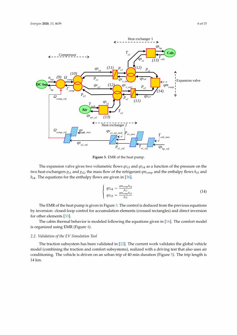
Figure 7. Measured and simulated energy consumption for the urban driving cycle.
3. Annual Variation in Energy Consumption for an Urban Driving Cycle
3.1. Case Study
Within the CUMIN program, an important objective is to have a precise estimate of the energy
needed to charge electric vehicles for commuters that come to the University of Lille. We thus take
this university campus as a case study. Lille is a city in Northern France. The climate is oceanic,
meaning that temperatures are moderate. In this study, the average daily minimal and maximal
temperature per month in 2018 are considered (Figure 8) [37]. This temperature varies from −1 °C
(February) to 16 °C (July) for the minimal daily temperature and 5 °C to 28 °C for the maximal daily
temperatures.
The energy consumption estimation is calculated for different daily commuting trips. The
outgoing trip is made in the morning around 7 a.m., and we assume this occurs when the temperature
is at its daily minimum. The return trip is assumed to occur at the maximal temperature around 5
p.m. The air conditioning subsystem is used when the temperature is higher than 25 °C, which occurs
only in July in Lille. The air conditioning must maintain the temperature 5 °C below the ambient
temperature. The heating subsystem is used when the temperature is below 13 °C and has an
objective to maintain a temperature of 20 °C in the cabin. These assumptions come from a behavioral
study from users of the University of Lille campus. While a more detailed analysis should be
conducted, this initial study provides a starting point for analysis.
Figure 6. Vehicle cabin temperature.
The energy consumption is simulated and compared with the energy calculated from the measuredbattery voltage and current (Figure 7). The measured velocity and ambient temperature have beenimposed as inputs for the simulation. The simulated energy consumption is 2.09 kWh versus 2.15 kWhfor the measured data. The final error on the energy consumption is about 3%.
Energies 2020, 13, 4639 8 of 15
Energies 2020, 13, x FOR PEER REVIEW 8 of 15
Figure 6. Vehicle cabin temperature.
The energy consumption is simulated and compared with the energy calculated from the
measured battery voltage and current (Figure 7). The measured velocity and ambient temperature
have been imposed as inputs for the simulation. The simulated energy consumption is 2.09 kWh
versus 2.15 kWh for the measured data. The final error on the energy consumption is about 3%.
Figure 7. Measured and simulated energy consumption for the urban driving cycle.
3. Annual Variation in Energy Consumption for an Urban Driving Cycle
3.1. Case Study
Within the CUMIN program, an important objective is to have a precise estimate of the energy
needed to charge electric vehicles for commuters that come to the University of Lille. We thus take
this university campus as a case study. Lille is a city in Northern France. The climate is oceanic,
meaning that temperatures are moderate. In this study, the average daily minimal and maximal
temperature per month in 2018 are considered (Figure 8) [37]. This temperature varies from −1 °C
(February) to 16 °C (July) for the minimal daily temperature and 5 °C to 28 °C for the maximal daily
temperatures.
The energy consumption estimation is calculated for different daily commuting trips. The
outgoing trip is made in the morning around 7 a.m., and we assume this occurs when the temperature
is at its daily minimum. The return trip is assumed to occur at the maximal temperature around 5
p.m. The air conditioning subsystem is used when the temperature is higher than 25 °C, which occurs
only in July in Lille. The air conditioning must maintain the temperature 5 °C below the ambient
temperature. The heating subsystem is used when the temperature is below 13 °C and has an
objective to maintain a temperature of 20 °C in the cabin. These assumptions come from a behavioral
study from users of the University of Lille campus. While a more detailed analysis should be
conducted, this initial study provides a starting point for analysis.
Figure 7. Measured and simulated energy consumption for the urban driving cycle.
3. Annual Variation in Energy Consumption for an Urban Driving Cycle
3.1. Case Study
Within the CUMIN program, an important objective is to have a precise estimate of the energyneeded to charge electric vehicles for commuters that come to the University of Lille. We thus take thisuniversity campus as a case study. Lille is a city in Northern France. The climate is oceanic, meaningthat temperatures are moderate. In this study, the average daily minimal and maximal temperatureper month in 2018 are considered (Figure 8) [37]. This temperature varies from −1 C (February) to16 C (July) for the minimal daily temperature and 5 C to 28 C for the maximal daily temperatures.
The energy consumption estimation is calculated for different daily commuting trips. The outgoingtrip is made in the morning around 7 a.m., and we assume this occurs when the temperature is at itsdaily minimum. The return trip is assumed to occur at the maximal temperature around 5 p.m. The airconditioning subsystem is used when the temperature is higher than 25 C, which occurs only in Julyin Lille. The air conditioning must maintain the temperature 5 C below the ambient temperature.The heating subsystem is used when the temperature is below 13 C and has an objective to maintain atemperature of 20 C in the cabin. These assumptions come from a behavioral study from users of theUniversity of Lille campus. While a more detailed analysis should be conducted, this initial studyprovides a starting point for analysis.Energies 2020, 13, x FOR PEER REVIEW 9 of 15
month
Temperature (°C) max min
Figure 8. Average minimal and maximal temperature per month in Lille in 2018 [37].
3.2. Generation of a Reference Driving Cycle
Measured driving cycles are affected by random conditions due to the driver, traffic jams and
stops at intersections. In this study, an ideal and constant driving cycle is used for each simulation step.
Additionally, driver behavior is isolated from other effects by assuming a fixed driver behavior using a
simple controller. Moreover, the thermal behavior of the battery is not considered in this study, which
has a minor effect for the considered temperature range [18]. This assumption can be studied later. This
setup allows for a fair comparison of the energy consumption between different scenarios that focuses
only on the HVAC and the route driven. The driving cycle is established for an average driving profile
by the driving generator developed in [22]. The generator takes data from the OpenstreetMap API [38]
to generate a driving cycle. Then this cycle is introduced into the simulation tool.
3.3. Annual Variation in Energy Consumption for an Urban Driving Cycle
The simulation is performed for every month of a complete year. This consumption is calculated
for an outgoing trip in the morning and for a return trip in the evening. The driving cycle is first
defined for a trip selected in a map-based interface (Figure 9a). Road data is used to provide the
velocity profile using the Driving Cycle Generator (Figure 9b). The velocity profile as well as the
ambient temperature are inputs for the vehicle simulation. The EMR has been transcribed into
Matlab-Simulink© thanks to the EMR library [34] (Figure 9c). The simulation process thus provides
an energy consumption estimate for a defined trip and ambient temperature.
The energy consumption for the urban driving cycle for the outgoing and return trips is
calculated for each month (Figure 10). Thus, the variation across months is attributable directly to use
of the HVAC subsystem. In the morning trip, the energy consumption increases up to 33% in
February due to heating requirements. For the return trip, the air conditioning increases the
consumption by 15% in July. Because of moderate temperatures in Lille, no air conditioning is
required except in July during the return trip. This result shows that taking into account the HVAC
subsystem can lead to additional consumption of energy that is non-trivial compared to the traction
energy, even in moderate climates like Northern France. This supplementary consumption will affect
the vehicle range, requiring more frequent charging. This point is important for drivers, but also for
the required charging infrastructure, especially if storage devices have to be included.
Figure 8. Average minimal and maximal temperature per month in Lille in 2018 [37].
3.2. Generation of a Reference Driving Cycle
Measured driving cycles are affected by random conditions due to the driver, traffic jams andstops at intersections. In this study, an ideal and constant driving cycle is used for each simulationstep. Additionally, driver behavior is isolated from other effects by assuming a fixed driver behaviorusing a simple controller. Moreover, the thermal behavior of the battery is not considered in this study,which has a minor effect for the considered temperature range [18]. This assumption can be studied later.This setup allows for a fair comparison of the energy consumption between different scenarios thatfocuses only on the HVAC and the route driven. The driving cycle is established for an average driving

Energies 2020, 13, 4639 9 of 15
profile by the driving generator developed in [22]. The generator takes data from the OpenstreetMapAPI [38] to generate a driving cycle. Then this cycle is introduced into the simulation tool.
3.3. Annual Variation in Energy Consumption for an Urban Driving Cycle
The simulation is performed for every month of a complete year. This consumption is calculatedfor an outgoing trip in the morning and for a return trip in the evening. The driving cycle is first definedfor a trip selected in a map-based interface (Figure 9a). Road data is used to provide the velocity profileusing the Driving Cycle Generator (Figure 9b). The velocity profile as well as the ambient temperatureare inputs for the vehicle simulation. The EMR has been transcribed into Matlab-Simulink© thanksto the EMR library [34] (Figure 9c). The simulation process thus provides an energy consumptionestimate for a defined trip and ambient temperature.
Energies 2020, 13, x FOR PEER REVIEW 10 of 15
a) Selected Urban trip
(University – Lille downtown)
Velocity (km/h)
distance (km)
c) Simulation tool (Matlab-Simulink © )
b) Deduced driving cycle
driving cycle
generator
Univ. Lille
Lille city Hall
Figure 9. Simulation process: (a) map-based trip selection, (b) deduced velocity profile, (c) vehicle
simulation.
Figure 10. Monthly variation in the EV energy consumption for the urban trip.
Figure 9. Simulation process: (a) map-based trip selection, (b) deduced velocity profile, (c) vehicle simulation.
The energy consumption for the urban driving cycle for the outgoing and return trips is calculatedfor each month (Figure 10). Thus, the variation across months is attributable directly to use of theHVAC subsystem. In the morning trip, the energy consumption increases up to 33% in February dueto heating requirements. For the return trip, the air conditioning increases the consumption by 15% in

Energies 2020, 13, 4639 10 of 15
July. Because of moderate temperatures in Lille, no air conditioning is required except in July duringthe return trip. This result shows that taking into account the HVAC subsystem can lead to additionalconsumption of energy that is non-trivial compared to the traction energy, even in moderate climateslike Northern France. This supplementary consumption will affect the vehicle range, requiring morefrequent charging. This point is important for drivers, but also for the required charging infrastructure,especially if storage devices have to be included.
Energies 2020, 13, x FOR PEER REVIEW 10 of 15
a) Selected Urban trip
(University – Lille downtown)
Velocity (km/h)
distance (km)
c) Simulation tool (Matlab-Simulink © )
b) Deduced driving cycle
driving cycle
generator
Univ. Lille
Lille city Hall
Figure 9. Simulation process: (a) map-based trip selection, (b) deduced velocity profile, (c) vehicle
simulation.
Figure 10. Monthly variation in the EV energy consumption for the urban trip. Figure 10. Monthly variation in the EV energy consumption for the urban trip.
4. Annual Variation in EV Energy Consumption Considering Different Commuting Trips
4.1. Studied Driving Cycles
Six daily trips are defined to represent different commuting trips to the University of Lille(Figure 11). These generated trips are associated with distinct residential areas where universitycommuters live. Their characteristics are summarized in Table 2.
Energies 2020, 13, x FOR PEER REVIEW 11 of 15
4. Annual Variation in EV Energy Consumption Considering Different Commuting Trips
4.1. Studied Driving Cycles
Six daily trips are defined to represent different commuting trips to the University of Lille
(Figure 11). These generated trips are associated with distinct residential areas where university
commuters live. Their characteristics are summarized in Table 2.
Figure 11. Different outgoing trips considered in this study.
Table 2. Characteristics of the six daily trips (one way).
Daily Trips Road Type Average Velocity (km/h) Distance (km) Duration (min)
1 Urban 28 7 15
2 Urban 34 4 7
3 Extra-urban 42 9 13
4 Extra-urban 49 16 20
5 Highway 69 27 23
6 Highway 89 20 13
4.2. Annual Variation in Energy Consumption
For each trip, energy consumption is calculated for each month with the simulation tool. These
results are presented to illustrate the variation in EV energy consumption across both commute types
and weather conditions.
4.2.1. Effect of the HVAC and Traction Subsystems on Consumption
First, the daily energy consumption of the traction subsystem (without HVAC) is calculated for
each trip (Figure 12). For a fair comparison of trips with different distances, this consumption is
represented in kWh per 100 km. The consumption is impacted by the velocity, which is the most
important factor for traction energy consumption, as already demonstrated in [22]. The number of
stops also had an impact on the traction consumption of the first trip, leading to a higher consumption
than trips 2 and 3.
Figure 11. Different outgoing trips considered in this study.

Energies 2020, 13, 4639 11 of 15
Table 2. Characteristics of the six daily trips (one way).
Daily Trips Road Type Average Velocity (km/h) Distance (km) Duration (min)
1 Urban 28 7 152 Urban 34 4 73 Extra-urban 42 9 134 Extra-urban 49 16 205 Highway 69 27 236 Highway 89 20 13
4.2. Annual Variation in Energy Consumption
For each trip, energy consumption is calculated for each month with the simulation tool.These results are presented to illustrate the variation in EV energy consumption across both commutetypes and weather conditions.
4.2.1. Effect of the HVAC and Traction Subsystems on Consumption
First, the daily energy consumption of the traction subsystem (without HVAC) is calculatedfor each trip (Figure 12). For a fair comparison of trips with different distances, this consumptionis represented in kWh per 100 km. The consumption is impacted by the velocity, which is the mostimportant factor for traction energy consumption, as already demonstrated in [22]. The number ofstops also had an impact on the traction consumption of the first trip, leading to a higher consumptionthan trips 2 and 3.Energies 2020, 13, x FOR PEER REVIEW 12 of 15
Figure 12. Energy consumption of the traction subsystem in the six sample trips.
The energy consumption of the vehicle including both traction and HVAC subsystems each
month is given in Figure 13a. for trips 1 and 6. The dashed lines represent the extremum of the energy
consumption for the two trips. The energy consumption of trip 1 is globally lower than trip 6.
However, the annual variation of trip 1 is larger. For trip 1, in June, the HVAC system is not used at
all, leading to the minimal energy consumption of the vehicle. In February, the consumption is
highest due to use of the HVAC system. The difference between the consumption of these two
months is 21% for trip 1. For trip 6, the variation is only about 8%. The six different trips are compared
in Figure 13b. The box represents the extremum of the consumption for each trip. The line inside the
box represents the median for the different trips. The variation in energy consumption is largest in
the urban trips due to the lower traction consumption and the higher time spent on the road
compared to the other trips. This is especially true in trip 1, which has more traffic stops that increase
the duration of the trip and represent time when the vehicle is heated but not driven.
Figure 13. (a) Energy consumption of the Electric Vehicle over 12 months of the year for trips 1 and 6.
The dashed lines represent the extremum of the energy consumption for each trip. (b) Energy
consumption of the Electric Vehicle for 6 different trips. The boxplot represents the extremum of the
energy consumption for the different trips. The lines inside the boxes represent the median.
4.2.2. Annual Consumption of the Electric Vehicle
Finally, the annual energy consumption is calculated (Figure 14). The yellow parts represent the
energy consumption of the traction subsystem while the dark blue bars represent the additional energy
used by the HVAC system. The HVAC system adds an average of 12% to the annual energy
consumption estimate without the HVAC system. The error varies from 5% for trip 6 to 21% for urban
trip 2. These results are for a location with a mild climate that neither requires significant heating nor
air conditioning and would be much higher for extreme cases of temperature variation, as in continental
climates. This work quantifies the contribution of HVAC energy use to overall consumption and
Figure 12. Energy consumption of the traction subsystem in the six sample trips.
The energy consumption of the vehicle including both traction and HVAC subsystems eachmonth is given in Figure 13a. for trips 1 and 6. The dashed lines represent the extremum of the energyconsumption for the two trips. The energy consumption of trip 1 is globally lower than trip 6. However,the annual variation of trip 1 is larger. For trip 1, in June, the HVAC system is not used at all, leadingto the minimal energy consumption of the vehicle. In February, the consumption is highest due touse of the HVAC system. The difference between the consumption of these two months is 21% fortrip 1. For trip 6, the variation is only about 8%. The six different trips are compared in Figure 13b.The box represents the extremum of the consumption for each trip. The line inside the box representsthe median for the different trips. The variation in energy consumption is largest in the urban trips dueto the lower traction consumption and the higher time spent on the road compared to the other trips.This is especially true in trip 1, which has more traffic stops that increase the duration of the trip andrepresent time when the vehicle is heated but not driven.

Energies 2020, 13, 4639 12 of 15
Energies 2020, 13, x FOR PEER REVIEW 12 of 15
Figure 12. Energy consumption of the traction subsystem in the six sample trips.
The energy consumption of the vehicle including both traction and HVAC subsystems each
month is given in Figure 13a. for trips 1 and 6. The dashed lines represent the extremum of the energy
consumption for the two trips. The energy consumption of trip 1 is globally lower than trip 6.
However, the annual variation of trip 1 is larger. For trip 1, in June, the HVAC system is not used at
all, leading to the minimal energy consumption of the vehicle. In February, the consumption is
highest due to use of the HVAC system. The difference between the consumption of these two
months is 21% for trip 1. For trip 6, the variation is only about 8%. The six different trips are compared
in Figure 13b. The box represents the extremum of the consumption for each trip. The line inside the
box represents the median for the different trips. The variation in energy consumption is largest in
the urban trips due to the lower traction consumption and the higher time spent on the road
compared to the other trips. This is especially true in trip 1, which has more traffic stops that increase
the duration of the trip and represent time when the vehicle is heated but not driven.
Figure 13. (a) Energy consumption of the Electric Vehicle over 12 months of the year for trips 1 and 6.
The dashed lines represent the extremum of the energy consumption for each trip. (b) Energy
consumption of the Electric Vehicle for 6 different trips. The boxplot represents the extremum of the
energy consumption for the different trips. The lines inside the boxes represent the median.
4.2.2. Annual Consumption of the Electric Vehicle
Finally, the annual energy consumption is calculated (Figure 14). The yellow parts represent the
energy consumption of the traction subsystem while the dark blue bars represent the additional energy
used by the HVAC system. The HVAC system adds an average of 12% to the annual energy
consumption estimate without the HVAC system. The error varies from 5% for trip 6 to 21% for urban
trip 2. These results are for a location with a mild climate that neither requires significant heating nor
air conditioning and would be much higher for extreme cases of temperature variation, as in continental
climates. This work quantifies the contribution of HVAC energy use to overall consumption and
Figure 13. (a) Energy consumption of the Electric Vehicle over 12 months of the year for trips 1and 6. The dashed lines represent the extremum of the energy consumption for each trip. (b) Energyconsumption of the Electric Vehicle for 6 different trips. The boxplot represents the extremum of theenergy consumption for the different trips. The lines inside the boxes represent the median.
4.2.2. Annual Consumption of the Electric Vehicle
Finally, the annual energy consumption is calculated (Figure 14). The yellow parts representthe energy consumption of the traction subsystem while the dark blue bars represent the additionalenergy used by the HVAC system. The HVAC system adds an average of 12% to the annual energyconsumption estimate without the HVAC system. The error varies from 5% for trip 6 to 21% for urbantrip 2. These results are for a location with a mild climate that neither requires significant heatingnor air conditioning and would be much higher for extreme cases of temperature variation, as incontinental climates. This work quantifies the contribution of HVAC energy use to overall consumptionand demonstrates that it is not trivial even in a favorable location like Lille, France. Estimates of energyconsumption should not neglect HVAC consumption in EVs, especially for urban trips.
Energies 2020, 13, x FOR PEER REVIEW 13 of 15
demonstrates that it is not trivial even in a favorable location like Lille, France. Estimates of energy
consumption should not neglect HVAC consumption in EVs, especially for urban trips.
Annual Consumption (kWh)
1 2 3 4 5 6
traction system consumption
HVAC consumption
Figure 14. Annual energy consumption of the Electric Vehicle in the 6 commuting trips.
5. Conclusions
A simulation tool was developed to study the energy consumption of EVs including energy
required for passenger comfort. This model has been validated through a comparison with measured
data from a real EV. An analysis of the energy consumption of an electric vehicle that includes the
comfort subsystem was performed for an oceanic climate with a temperature variation between −1 °C
and 28 °C for different daily trips. The results show the relevance of both driving cycles and climate
conditions to energy consumption. Average vehicle velocity has a large effect when the different trips
are compared. At the same time, the ambient temperature leads to a higher variation in all types of
travel, especially for urban trips, due to the use of the HVAC subsystem. The results for the campus
case study here shows an increase in consumption up to 33% in winter due to cabin heating and up
to 15% in the summer due to air conditioning. Greater amounts of charging energy should thus be
expected in these periods.
Generated driving cycles are used in order to directly and fairly compare between different trips.
Consequently, no traffic congestion, no random stops, and no driver effects impacting the driving
profile have been considered. These random conditions add even more variation to the energy
consumption of the vehicle as they impact both traction and HVAC subsystem consumption. For a
daily driving range estimator, the generated driving cycle should be as realistic as possible. This
generator can be improved to take into account traffic and driver behavior effects.
In this work, there are several important caveats. First, the analysis focuses on daily commuting
trips to the campus of the University of Lille. Reality is more complex as other trips are normally
made for different purposes (shopping, collecting children, etc.). Thus, the work can be expanded to
other trip types to understand the diversity of trips made by users. The study in this article has
addressed a limited temperature range in a moderate climate. The results of this study cannot be
directly applied in other climates, particularly for extreme climatic conditions. Moreover, the
consumption of the HVAC subsystem increases rapidly when the temperature is below 0 °C and
higher than 30 °C [14,15]. Overall, applying these methods outside the mild oceanic climate of Lille
should demonstrate stronger effects. In order to extend this to other climates with broader
temperature range, two improvements should be pursued. First, a thermal model of the battery
should be included as the energy storage and losses are affected at low and high temperature. Second,
the control strategies of the HVAC subsystem should be studied in detail because other comfort
strategies may be more appropriate for extreme temperature values (such as battery heating).
Figure 14. Annual energy consumption of the Electric Vehicle in the 6 commuting trips.
5. Conclusions
A simulation tool was developed to study the energy consumption of EVs including energyrequired for passenger comfort. This model has been validated through a comparison with measureddata from a real EV. An analysis of the energy consumption of an electric vehicle that includes thecomfort subsystem was performed for an oceanic climate with a temperature variation between −1 C

Energies 2020, 13, 4639 13 of 15
and 28 C for different daily trips. The results show the relevance of both driving cycles and climateconditions to energy consumption. Average vehicle velocity has a large effect when the different tripsare compared. At the same time, the ambient temperature leads to a higher variation in all types oftravel, especially for urban trips, due to the use of the HVAC subsystem. The results for the campuscase study here shows an increase in consumption up to 33% in winter due to cabin heating and upto 15% in the summer due to air conditioning. Greater amounts of charging energy should thus beexpected in these periods.
Generated driving cycles are used in order to directly and fairly compare between different trips.Consequently, no traffic congestion, no random stops, and no driver effects impacting the driving profilehave been considered. These random conditions add even more variation to the energy consumptionof the vehicle as they impact both traction and HVAC subsystem consumption. For a daily drivingrange estimator, the generated driving cycle should be as realistic as possible. This generator can beimproved to take into account traffic and driver behavior effects.
In this work, there are several important caveats. First, the analysis focuses on daily commutingtrips to the campus of the University of Lille. Reality is more complex as other trips are normally madefor different purposes (shopping, collecting children, etc.). Thus, the work can be expanded to othertrip types to understand the diversity of trips made by users. The study in this article has addressed alimited temperature range in a moderate climate. The results of this study cannot be directly applied inother climates, particularly for extreme climatic conditions. Moreover, the consumption of the HVACsubsystem increases rapidly when the temperature is below 0 C and higher than 30 C [14,15]. Overall,applying these methods outside the mild oceanic climate of Lille should demonstrate stronger effects.In order to extend this to other climates with broader temperature range, two improvements should bepursued. First, a thermal model of the battery should be included as the energy storage and losses areaffected at low and high temperature. Second, the control strategies of the HVAC subsystem should bestudied in detail because other comfort strategies may be more appropriate for extreme temperaturevalues (such as battery heating).
To conclude, this study quantitatively shows the importance of accounting for the effect of ambienttemperature on the energy consumption for daily trips or estimation of the vehicle range. This isrelevant for drivers but also for evaluating the design of infrastructure needed to charge a fleet ofvehicles. Further works should now be realized to consider the effects of driver behaviors and trafficjams on energy consumption independently of other effects. Then, all effects could be coupled in acomprehensive model.
Author Contributions: Conceptualization, A.D. and A.B.; methodology and software, A.D.; software validation,A.D. and A.B.; resources, A.D., E.C. and G.-M.S.; writing—original draft preparation, A.D.; writing—review andediting, E.H., A.B., R.T., E.C. and G.-M.S.; supervision, A.B., E.C. and R.T.; funding acquisition, A.B.; All authorshave read and agreed to the published version of the manuscript.
Funding: This paper has been realized thanks to the funding of the Region “Hauts-de-France” (Northern France)and University of Lille within the CUMIN program. Moreover, it has been realized within the framework of thePANDA project which has received funding from the European Union’s Horizon 2020 research and innovationprogram under grant agreement no. 824256 (PANDA).
Conflicts of Interest: The authors declare no conflict of interest.
References
1. Van Mierlo, J.; Messagie, M.; Rangaraju, S. Comparative environmental assessment of alternative fueledvehicles using a life cycle assessment. Transp. Res. Procedia 2017, 25, 3435–3445. [CrossRef]
2. Tucki, K.; Orynycz, O.; Swic, A.; Mitoraj-Wojtanek, M. The Development of Electromobility in Poland andEU States as a Tool for Management of CO2 Emissions. Energies 2019, 12, 2942. [CrossRef]
3. Global EV Outlook 2020, Entering the Decade of Electric Drive? International Energy Agency Report; InternationalEnergy Agency: Paris, France, 2020.
4. C40 Cities Organization. Fossil Fuel Free Streets Declaration. Available online: https://www.c40.org/other/green-and-healthy-streets (accessed on 20 July 2020).

Energies 2020, 13, 4639 14 of 15
5. Bouscayrol, A.; Castex, E.; Desreveaux, A.; Ferla, O.; Frotey, J.; German, R.; Lhomme, W.; Sergent, J.F. Campusof University with Mobility based on Innovation and carbon Neutral. In Proceedings of the 2017 IEEEVehicle Power and Propulsion, Belfort, France, 11–14 December 2017.
6. Neubauer, J.; Wood, E. The impact of range anxiety and home, workplace, and public charging infrastructureon simulated battery electric vehicle lifetime utility. J. Power Sources 2014, 257, 12–20. [CrossRef]
7. Giansoldati, M.; Danielis, R.; Rotaris, L.; Scorrano, M. The role of driving range in consumers’ purchasingdecision for electric cars in Italy. Energy 2018, 165, 267–274. [CrossRef]
8. Higueras-Castillo, E.; Molinillo, S.; Coca-Stefaniak, J.A.; Liébana-Cabanillas, F. Perceived Value and CustomerAdoption of Electric and Hybrid Vehicles. Sustainability 2019, 11, 4956. [CrossRef]
9. Kim, S.; Lee, J.; Lee, C. Does Driving Range of Electric Vehicles Influence Electric Vehicle Adoption?Sustainability 2017, 9, 1783. [CrossRef]
10. Rauh, N.; Franke, T.; Krems, J.F. User experience with electric vehicles while driving in a critical rangesituation—a qualitative approach. IET Intell. Transp. Syst. 2015, 9, 734–739. [CrossRef]
11. Eisel, M.; Nastjuk, I.; Kolbe, L.M. Understanding the influence of in-vehicle information systems on rangestress—Insights from an electric vehicle field experiment. Transp. Res. Part F Traffic Psychol. Behav. 2016, 43,199–211. [CrossRef]
12. Varga, B.O.; Sagoian, A.; Mariasiu, F. Prediction of Electric Vehicle Range: A Comprehensive Review ofCurrent Issues and Challenge. Energies 2019, 12, 946. [CrossRef]
13. Yi, Z.; Bauer, P.H. Effects of environmental factors on electric vehicle energy consumption: A sensitivityanalysis. IET Electr. Syst. Transp. 2017, 7, 3–13. [CrossRef]
14. Kambly, K.; Bradley, T.H. Geographical and temporal differences in electric vehicle range due to cabinconditioning energy consumption. J. Power Sources 2015, 275, 468–475. [CrossRef]
15. Yuksel, T.; Michalek, J.J. Effects of regional temperature on electric vehicle efficiency, range, and emissions inthe United States. Environ. Sci. Technol. 2015, 49, 3974–3980. [CrossRef] [PubMed]
16. Horrein, L.; Bouscayrol, A.; Lhomme, W.; Depature, C. Impact of Heating System on the Range of an ElectricVehicle. IEEE Trans. Veh. Technol. 2017, 66, 4668–4677. [CrossRef]
17. Lindgren, J.; Lund, P.D. Effect of extreme temperatures on battery charging and performance of electricvehicles. J. Power Sources 2016, 328, 37–45. [CrossRef]
18. German, R.; Shili, S.; Desreveaux, A.; Sari, A.; Venet, P.; Bouscayrol, A. Dynamical Coupling of a BatteryElectro-Thermal Model and the Traction Model of an EV for Driving Range Simulation. IEEE Trans.Veh. Technol. 2020, 69, 328–337. [CrossRef]
19. Jaguemont, J.; Boulon, L.; Dubé, Y. A comprehensive review of lithium-ion batteries used in hybrid andelectric vehicles at cold temperature. Appl. Energy 2016, 164, 99–114. [CrossRef]
20. Desreveaux, A.; Bouscayrol, A.; Trigui, R.; Castex, E.; Klein, J. Impact of the Traffic Stops on the EnergyConsumption of Electric Vehicles. In Proceedings of the 32nd Electric Vehicle Symposium, Lyon, France,19–22 May 2019.
21. Fernández, R.A.; Caraballo, S.C.; López, F.C. A probabilistic approach for determining the influence of urbantraffic management policies on energy consumption and greenhouse gas emissions from a battery electricvehicle. J. Clean. Prod. 2019, 236, 117604. [CrossRef]
22. Desreveaux, A.; Bouscayrol, A.; Trigui, R.; Castex, E.; Klein, J. Impact of the Velocity Profile on the EnergyConsumption of Electric Vehicle. IEEE Trans. Veh. Technol. 2019, 68, 11420–11426. [CrossRef]
23. Fiori, C.; Arcidiacono, V.; Fontaras, G.; Makridis, M.; Mattas, K.; Marzano, V.; Thiel, C.; Ciuffo, B. The effectof electrified mobility on the relationship between traffic conditions and energy consumption. Transp. Res.Part D Transp. Environ. 2019, 67, 275–290. [CrossRef]
24. Neubauer, J.; Wood, E. Thru-life impacts of driver aggression, climate, cabin thermal management, andbattery thermal management on battery electric vehicle utility. J. Power Sources 2014, 259, 262–275. [CrossRef]
25. Liu, K.; Wang, J.; Yamamoto, T.; Morikawa, T. Modeling the multilevel structure and mixed effects of thefactors influencing the energy consumption of electric vehicles. Appl. Energy 2016, 183, 1351–1360. [CrossRef]
26. De Cauwer, C.; Verbeke, W.; Coosemans, T.; Faid, S.; Van Mierlo, J. A data-driven method for energyconsumption prediction and energy-efficient routing of electric vehicles in real-world conditions. Energies2017, 10, 608. [CrossRef]
27. Chan, C.C.; Bouscayrol, A.; Chen, K. Electric, hybrid, and fuel-cell vehicles: Architectures and modeling.IEEE Trans. Veh. Technol. 2010, 59, 589–598. [CrossRef]

Energies 2020, 13, 4639 15 of 15
28. Baouche, F.; Billot, R.; Trigui, R.; El Faouzi, N.E. Efficient Allocation of Electric Vehicles Charging Stations:Optimization Model and Application to a Dense Urban Network. IEEE Intell. Trans. Syst. Mag. 2014, 6,33–43. [CrossRef]
29. Joud, L.; Da Silva, R.; Chrenko, D.; Kéromnès, A.; Le Moyne, L. Smart Energy Management for Series HybridElectric Vehicles Based on Driver Habits Recognition and Prediction. Energies 2020, 13, 2954. [CrossRef]
30. Chen, Z.; Lu, J.; Liu, B.; Zhou, N.; Li, S. Optimal Energy Management of Plug-In Hybrid Electric VehiclesConcerning the Entire Lifespan of Lithium-Ion Batteries. Energies 2020, 13, 2543. [CrossRef]
31. Renault, Z. Available online: http://www.renault.fr/vehicules/vehicules-electriques/zoe (accessed on20 July 2020).
32. Mayet, C.; Horrein, L.; Bouscayrol, A.; Delarue, P.; Verhille, J.N.; Chattot, E.; Lemaire-Semail, B. Comparisonof Different Models and Simulation Approaches for the Energetic Study of a Subway. IEEE Trans. Veh. Technol.2014, 63, 556–565. [CrossRef]
33. Bouscayrol, A.; Hautier, J.P.; Lemaire-Semail, B. Graphic Formalisms for the Control of Multi-Physical EnergeticSystems. Systemic Design Methodologies for Electrical Energy, Tome 1, Analysis, Synthesis and Management;Roboam, X., Ed.; ISTE: London, UK; Willey: Hoboken, NJ, USA, 2012; Chapter 3, ISBN 9781848213883.
34. EMR Website. Available online: https://www.emrwebsite.org/ (accessed on 20 July 2020).35. Martínez-García, M.; Zhang, Y.; Gordon, T. Modeling Lane Keeping by a Hybrid Open-Closed-Loop Pulse
Control Scheme. IEEE Trans. Ind. Inf. 2016, 12, 2256–2265. [CrossRef]36. Zhang, Q.; Stockar, S.; Canova, M. Energy-Optimal Control of an Automotive Air Conditioning System for
Ancillary Load Reduction. IEEE Trans. Control Syst. Technol. 2016, 24, 67–80. [CrossRef]37. Weather Data in Lille in 2018. Available online: https://www.meteofrance.fr (accessed on 20 July 2020).38. OpenStreetMap API. Available online: https://api.openstreetmap.org (accessed on 20 July 2020).
© 2020 by the authors. Licensee MDPI, Basel, Switzerland. This article is an open accessarticle distributed under the terms and conditions of the Creative Commons Attribution(CC BY) license (http://creativecommons.org/licenses/by/4.0/).