electric vehicle projections 2021
TRANSCRIPT

Electric vehicle projections 2021
Paul Graham and Lisa Havas
May 2021
Australia’s National Science Agency

Electric vehicle projections 2021 | i
Citation
Graham, P.W. and Havas, L. 2021, Electric vehicle projections 2021, CSIRO, Australia.
Copyright
© Commonwealth Scientific and Industrial Research Organisation 2021. To the extent permitted
by law, all rights are reserved and no part of this publication covered by copyright may be
reproduced or copied in any form or by any means except with the written permission of CSIRO.
Important disclaimer
CSIRO advises that the information contained in this publication comprises general statements
based on scientific research. The reader is advised and needs to be aware that such information
may be incomplete or unable to be used in any specific situation. No reliance or actions must
therefore be made on that information without seeking prior expert professional, scientific and
technical advice. To the extent permitted by law, CSIRO (including its employees and consultants)
excludes all liability to any person for any consequences, including but not limited to all losses,
damages, costs, expenses and any other compensation, arising directly or indirectly from using this
publication (in part or in whole) and any information or material contained in it.
CSIRO is committed to providing web accessible content wherever possible. If you are having
difficulties with accessing this document please contact [email protected].

Electric vehicle projections 2021 | i
Contents Acknowledgments ........................................................................................................................... iv
Executive summary ......................................................................................................................... v
1 Introduction ........................................................................................................................ 1
2 Methodology ...................................................................................................................... 2
2.1 Adoption projections method overview ............................................................... 2
2.2 Demographic factors and weights ......................................................................... 8
2.3 Role of economic growth in projection method ................................................... 9
3 Scenario definitions .......................................................................................................... 10
3.2 Financial and non-financial scenario drivers ....................................................... 14
4 Data assumptions ............................................................................................................. 23
4.1 Technology costs ................................................................................................. 23
4.2 Electricity tariffs ................................................................................................... 25
4.3 Income and population growth ........................................................................... 27
4.4 Separate dwellings and home ownership ........................................................... 28
4.5 Vehicle market segmentation ............................................................................. 30
4.6 Vehicle to home or grid ....................................................................................... 35
4.7 Shares of electric vehicle charging behaviour ..................................................... 36
4.8 Transport demand ............................................................................................... 36
4.9 Non-road electrification ...................................................................................... 42
5 Projections results ............................................................................................................ 44
5.1 Sales and fleet share ............................................................................................ 44
5.2 Electric vehicle numbers and consumption ........................................................ 46
5.3 Charging profiles .................................................................................................. 51
Additional data assumptions ............................................................................... 53
Shortened forms ........................................................................................................................... 54
References ............................................................................................................................. 57
Figures
Figure 2-1 Historical and projected electric vehicle sales by state to 2022, Current Trajectory
scenario ........................................................................................................................................... 3
Figure 2-2: Overview of transport demand model ......................................................................... 4
ii | CSIRO Australia’s National Science Agency
Figure 2-3 Adoption model methodology overview ....................................................................... 7
Figure 4-1 Assumed share of separate dwellings in total dwelling stock by scenario ................. 29
Figure 4-2 Historical (ABS Census) and projected share of homes owned outright or mortgaged,
source AIHW (2017) ...................................................................................................................... 30
Figure 4-3 Historical and projected passenger transport demand ............................................... 37
Figure 4-4 Historical and projected freight transport demand .................................................... 37
Figure 4-5 Share of passenger and freight autonomous vehicles in the road vehicle fleet by
scenario by 2050 ........................................................................................................................... 39
Figure 4-6 Comparison of 2018-19 and 2019-20 vehicle utilisation by vehicle type ................... 40
Figure 4-7 Historical and projected national road vehicle kilometres travelled, all road modes 41
Figure 4-8 Projected national road vehicle fleet by scenario ....................................................... 42
Figure 5-1 Projected sales share, all electric vehicles, compared to selected 2020 projections . 45
Figure 5-2 Projected fleet share, all electric vehicles, compared to selected 2020 projections .. 46
Figure 5-3 Projected number of BEVs in the NEM ........................................................................ 47
Figure 5-4 Projected number of BEVs in the SWIS ....................................................................... 47
Figure 5-5 Projected number of vehicles in the NEM by 2050, all electric vehicles by type ........ 48
Figure 5-6 Projected number of vehicles in the SWIS by 2050, all electric vehicles by type ....... 49
Figure 5-7 Projected electricity consumption by BEVs in the NEM .............................................. 50
Figure 5-8 Projected electricity consumption by BEVs in the SWIS.............................................. 50
Figure 5-9 Average daily charging profiles for light passenger vehicles ....................................... 51
Figure 5-10 Average daily charging profiles for rigid trucks ......................................................... 52
Apx Figure A.1 Electric vehicle fuel efficiency by road mode ....................................................... 53
Tables
Table 2-1 Weights and factors for electric vehicles ........................................................................ 9
Table 3-1 AEMO scenario definitions ............................................................................................ 12
Table 3-2 Extended scenario definitions ....................................................................................... 14
Table 3-3: Economic drivers of electric and fuel cell electric vehicles (FCEV) and approach to
including them in scenarios .......................................................................................................... 15
Table 3-4: Economic drivers of autonomous private and ride share vehicles and approach to
including them in scenarios .......................................................................................................... 16
Table 3-5: Infrastructure drivers for electric and fuel cell vehicles and approach to including
them in scenarios .......................................................................................................................... 17

Electric vehicle projections 2021 | iii
Table 3-6 Emerging or potential disruptive business models to support embedded technology
adoption ........................................................................................................................................ 18
Table 3-7 Electric vehicle policy settings by scenario ................................................................... 22
Table 4-1 Current Trajectory scenario internal combustion and electric vehicle cost
assumptions, 2020 $’000 .............................................................................................................. 24
Table 4-2 Average annual percentage growth in GSP to 2050 by state and scenario, source:
AEMO and economic consultant .................................................................................................. 28
Table 4-3 Average annual percentage rate of growth in customers to 2050 by state and scenario
(Pre-COVID-19), source: AEMO and economic consultant ........................................................... 28
Table 4-4 Non-financial limitations on electric and fuel cell vehicle uptake and the calculated
maximum market share ................................................................................................................ 32
Table 4-5 Shares of different electric vehicle charging behaviours by 2050 based on limiting
factor analysis ............................................................................................................................... 34
Table 4-6 Assumed changes in vehicle utilisation and rationale .................................................. 40
Table 4-7 Rail freight and aviation electrification assumptions ................................................... 43

iv | CSIRO Australia’s National Science Agency
Acknowledgments
This report has benefited from input from AEMO staff and the AEMO Forecasting Reference
Group.
Electric vehicle projections 2021 | v
Executive summary
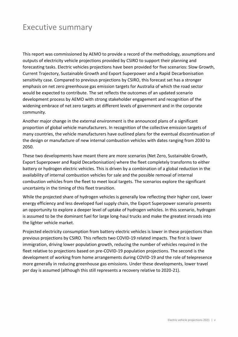
This report was commissioned by AEMO to provide a record of the methodology, assumptions and
outputs of electricity vehicle projections provided by CSIRO to support their planning and
forecasting tasks. Electric vehicles projections have been provided for five scenarios: Slow Growth,
Current Trajectory, Sustainable Growth and Export Superpower and a Rapid Decarbonisation
sensitivity case. Compared to previous projections by CSIRO, this forecast set has a stronger
emphasis on net zero greenhouse gas emission targets for Australia of which the road sector
would be expected to contribute. The set reflects the outcomes of an updated scenario
development process by AEMO with strong stakeholder engagement and recognition of the
widening embrace of net zero targets at different levels of government and in the corporate
community.
Another major change in the external environment is the announced plans of a significant
proportion of global vehicle manufacturers. In recognition of the collective emission targets of
many countries, the vehicle manufacturers have outlined plans for the eventual discontinuation of
the design or manufacture of new internal combustion vehicles with dates ranging from 2030 to
2050.
These two developments have meant there are more scenarios (Net Zero, Sustainable Growth,
Export Superpower and Rapid Decarbonisation) where the fleet completely transforms to either
battery or hydrogen electric vehicles. This is driven by a combination of a global reduction in the
availability of internal combustion vehicles for sale and the possible removal of internal
combustion vehicles from the fleet to meet local targets. The scenarios explore the significant
uncertainty in the timing of this fleet transition.
While the projected share of hydrogen vehicles is generally low reflecting their higher cost, lower
energy efficiency and less developed fuel supply chain, the Export Superpower scenario presents
an opportunity to explore a deeper level of uptake of hydrogen vehicles. In this scenario, hydrogen
is assumed to be the dominant fuel for large long-haul trucks and make the greatest inroads into
the lighter vehicle market.
Projected electricity consumption from battery electric vehicles is lower in these projections than
previous projections by CSIRO. This reflects two COVID-19 related impacts. The first is lower
immigration, driving lower population growth, reducing the number of vehicles required in the
fleet relative to projections based on pre-COVID-19 population projections. The second is the
development of working from home arrangements during COVID-19 and the role of telepresence
more generally in reducing greenhouse gas emissions. Under these developments, lower travel
per day is assumed (although this still represents a recovery relative to 2020-21).

Electric vehicle projections 2021 | 1
1 Introduction
Each year, AEMO requires updated projections of electric vehicle adoption and operation of
electric vehicle chargers for input into various planning and forecasting tasks. CSIRO has been
commissioned to provide electric vehicles projections for five scenarios: Slow Growth, Current
Trajectory, Net Zero, Sustainable Growth and Export Superpower and a Rapid Decarbonisation
sensitivity case. These are described further in the body of this report.
The report is set out in five sections. Section 2 provides a description of the applied projection
methodology. Section 3 describes the scenarios and their broad settings. Section 4 outlines the
scenario assumptions in detail and the projections are presented in Section 5.
2 | CSIRO Australia’s National Science Agency
2 Methodology
2.1 Adoption projections method overview
The projections undertaken are for periods of months, years and decades. Consequently, the
projection approach needs to be robust over both shorter- and longer-term projection periods.
The longer term adoption projections are based on a fundamental model of relevant drivers that
includes human behaviour and physical drivers and constraints. While these models are sound,
long term adoption models can overlook short term variations due to imperfect information,
unexpected shifts in key drivers and delays in observing the current state of the market. To
improve the short-term performance of the adoption models, the approach should ideally include
a second more accurate shorter-term projection approach to adjust for short term variations in
the EV market.
Short term projection approaches tend to be based on extrapolation of recent activity without
considering the fundamental drivers. These include regression analysis and other types of trend
analysis. While trend analysis generally performs best in the short term, extrapolating a simple
trend indefinitely leads to poor projection results as fundamental drivers or constraints on the
activity will assert themselves over time, shifting the activity away from past trends.
Based on these observations about the performance of short- and long-term projection
approaches, and our requirement to deliver both long and short term projections, this report
applies a combination of a short-term trend model and a long-term based transport demand and
technology adoption model.
Other than population, economic growth and assumptions about road vehicle demand, CSIRO
made no special allowance in the projections for COVID-19 pandemic impacts. Historical data
suggests electric vehicle sales were not impacted in 2020 (despite national vehicle sales of all
vehicles falling significantly).
2.1.1 Trend model
For the period between June 2019-20 and June 2021-22, trend analysis is applied to produce
projections based on historical data. The ABS motor vehicle census1 is applied and is considered
the most appropriate data set to capture current vehicle numbers, as alternative data sets appear
to contain missing data. CSIRO adjusts the sales data from other sources (e.g. the FCAI VFACTS) to
align with the identified ABS EV fleet.
The EV trend is estimated as a linear regression against a minimum of 3 years of state annual sales
data or up to 5 years for regions where the sales were too volatile to rely too heavily on only
recent data. A separate regression is run for plug-in hybrid and battery electric vehicles (PHEVs
1 Available at: https://www.abs.gov.au/statistics/industry/tourism-and-transport/motor-vehicle-census-australia
Electric vehicle projections 2021 | 3
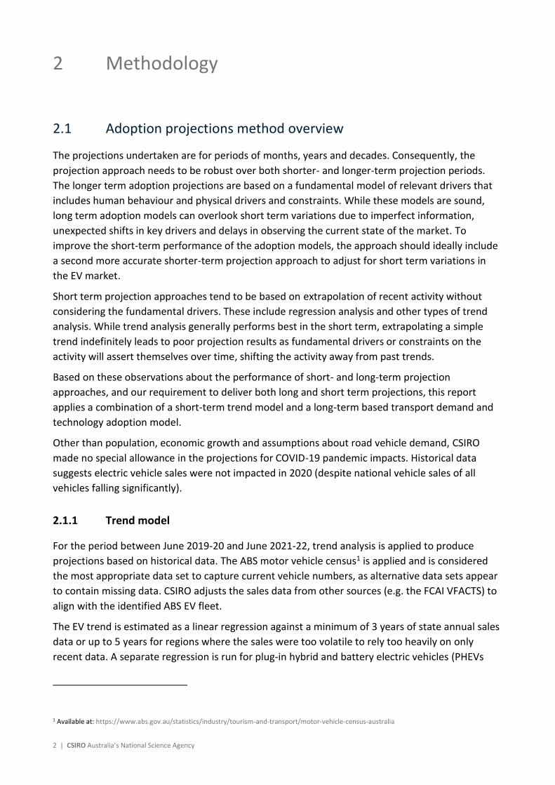
and BEVs). Figure 2-1 shows the projections from the trend analysis. The ACT has experienced a
recent jump in sales reflecting its introduction of the largest stamp duty rebates available in
Australia for electric vehicles.
The trend model also applies some variation between scenarios in the short-term to capture
uncertainty during this period. The Current Trajectory and Net Zero scenarios assume the
underlying trend remains unchanged while the trend for Slow Growth is adjusted downwards by
10% and the trend for the remainder of the scenarios is adjusted upwards to a maximum of 20%.
This captures the potential for stronger non-linear growth trends in the short term. The ranges are
based on the author’s judgement of the degree of upside and downside uncertainty in the trend.
Figure 2-1 Historical and projected electric vehicle sales by state to 2022, Current Trajectory scenario
2.1.2 Transport demand model
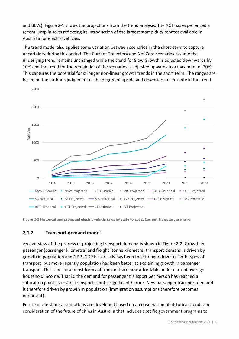
An overview of the process of projecting transport demand is shown in Figure 2-2. Growth in
passenger (passenger kilometre) and freight (tonne kilometre) transport demand is driven by
growth in population and GDP. GDP historically has been the stronger driver of both types of
transport, but more recently population has been better at explaining growth in passenger
transport. This is because most forms of transport are now affordable under current average
household income. That is, the demand for passenger transport per person has reached a
saturation point as cost of transport is not a significant barrier. New passenger transport demand
is therefore driven by growth in population (immigration assumptions therefore becomes
important).
Future mode share assumptions are developed based on an observation of historical trends and
consideration of the future of cities in Australia that includes specific government programs to
0
500
1000
1500
2000
2500
2014 2015 2016 2017 2018 2019 2020 2021 2022
Veh
icle
s
NSW Historical NSW Projected VIC Historical VIC Projected QLD Historical QLD Projected
SA Historical SA Projected WA Historical WA Projected TAS Historical TAS Projected
ACT Historical ACT Projected NT Historical NT Projected
4 | CSIRO Australia’s National Science Agency
extend airports, rail and road infrastructure. For the non-road sectors, fuel consumption
projections are based on multiplying projected demand by long term trends in fuel efficiency. In
the past CSIRO would include some changes in mode shares over time . For example, historically,
aviation had been steadily capturing more of the passenger share market. However, the COVID-19
pandemic has interrupted and reversed some of these trends. As a conservative approach, the
mode shares for passenger transport are mostly held constant at their current levels with only a
slight leaning towards previous trends. Freight transport mode shares were less impacted by
COVID-19 and so their historical trends in mode share are allowed to continue (Section 4.8 shows
the impact of these assumptions).
Figure 2-2: Overview of transport demand model
There are several more steps in projecting road sector transport demand. The first additional step
is that the demand model takes cost of travel information from the adoption model and applies a
price elasticity to demand of -0.22. That is, if the cost of road transport (passenger or freight) is
expected to fall by 10% this will lead to 2% increase in road transport demand. Conversely a 10%
increase in cost of travel would lead to a 2% decrease in transport demand. Cost of travel is
measured in dollars per kilometre and includes the whole cost of vehicle ownership and operation.
The main driver of rising transport costs in the future is expected to be fuel prices. However,
2 Transport demand elasticities have been studied for many decades. This site summarises available evidence: https://www.bitre.gov.au/databases/tedb
Additional sector calculations
Road: Cost of travel elasticity and changes in passengers/tonnes per vehicle and trip length
Non-road: Future trends on fuel efficiency and fuel shares
Apply mode share assumptions
Passenger – active, road, rail, air Freight – road, rail, air, shipping
Apply macroeconomic drivers
Passenger – population growth Freight – GDP growth

Electric vehicle projections 2021 | 5
improved fuel efficiency and higher vehicle utilisation from vehicle electrification and autonomous
vehicles respectively could see costs fall.
The second additional step is to take account of changes in the vehicle load. For example, a
decrease in passengers per vehicle implies more vehicle kilometres will be required to meet total
demand for passenger kilometres. Similarly, an increase in tonnes per vehicle capacity would
mean fewer vehicles were required to meet freight tonne kilometre demand. Tonnes per vehicle
are held constant over time for freight vehicles. Passengers per vehicle increases if the adoption
model projects greater adoption of rideshare services.
The final step takes account of changes in trip length which is measured in aggregate by kilometres
per vehicle. Kilometres per vehicle is varied to take account of changes due to the impact of
COVID-19 and of autonomous vehicles and ride sharing. COVID-19 has reduced average kilometres
per vehicle for passenger vehicles. Alternative assumptions are imposed, depending on the
scenario, about how much kilometres per vehicle recovers. In some scenarios, where there is a
strong greenhouse gas abatement imperative, it is assumed that kilometres per vehicle remains
lower in the longer term to support greater use of telepresence as an abatement measure.
The model projects the uptake of autonomous vehicles and ridesharing and their impact on
transport demand. Ride sharing increases the number of passengers per vehicle which on face
value reduces the amount of vehicle kilometres needed to meet passenger kilometre demand and
this is taken account of in the previous step. However, the most convenient service3 would pick up
and drop off each passenger at their destination meaning that each passenger takes a longer trip
than if they had used a non-ride sharing mode. These extra kilometres associated with ride sharing
trips are considered in this step.
2.1.3 Consumer technology adoption model
The consumer technology adoption curve is a whole of market scale property that is exploited for
the purposes of projecting adoption, particularly in markets for new products. The theory posits
that technology adoption will be led by an early adopter group who, despite high payback periods,
are driven to invest by other motivations such as values, autonomy and enthusiasm for new
technologies. As time passes, fast followers or the early majority take over and this is the most
rapid period of adoption. In the latter stages the late majority or late followers may still be holding
back due to constraints they may not be able to overcome, nor wish to overcome even if the
product is attractively priced. These early concepts were developed by authors such as Rogers
(1962) and Bass (1969).
Over the last 50 years, a wide range of applications seeking to use this as a projection tool have
experimented with a combination of price and non-price drivers to calibrate the shape of the
adoption curve for any given context. Price can be included directly or as a payback period or
return on investment. The adoption curve is developed by applying a payback period and a
3 Note that the Australian version of UberPool currently does not directly pick up and drop off at your desired points. Rather it includes some walking to connect you with the route an existing vehicle is travelling and may include some walking after drop-off. However, some overseas version include point to point drop-off and pick-up. https://www.uber.com/en-AU/ride/uberpool/
6 | CSIRO Australia’s National Science Agency
maximum market share assumption. Data on these two inputs are required to calibrate the shape
of the logistic curve function.
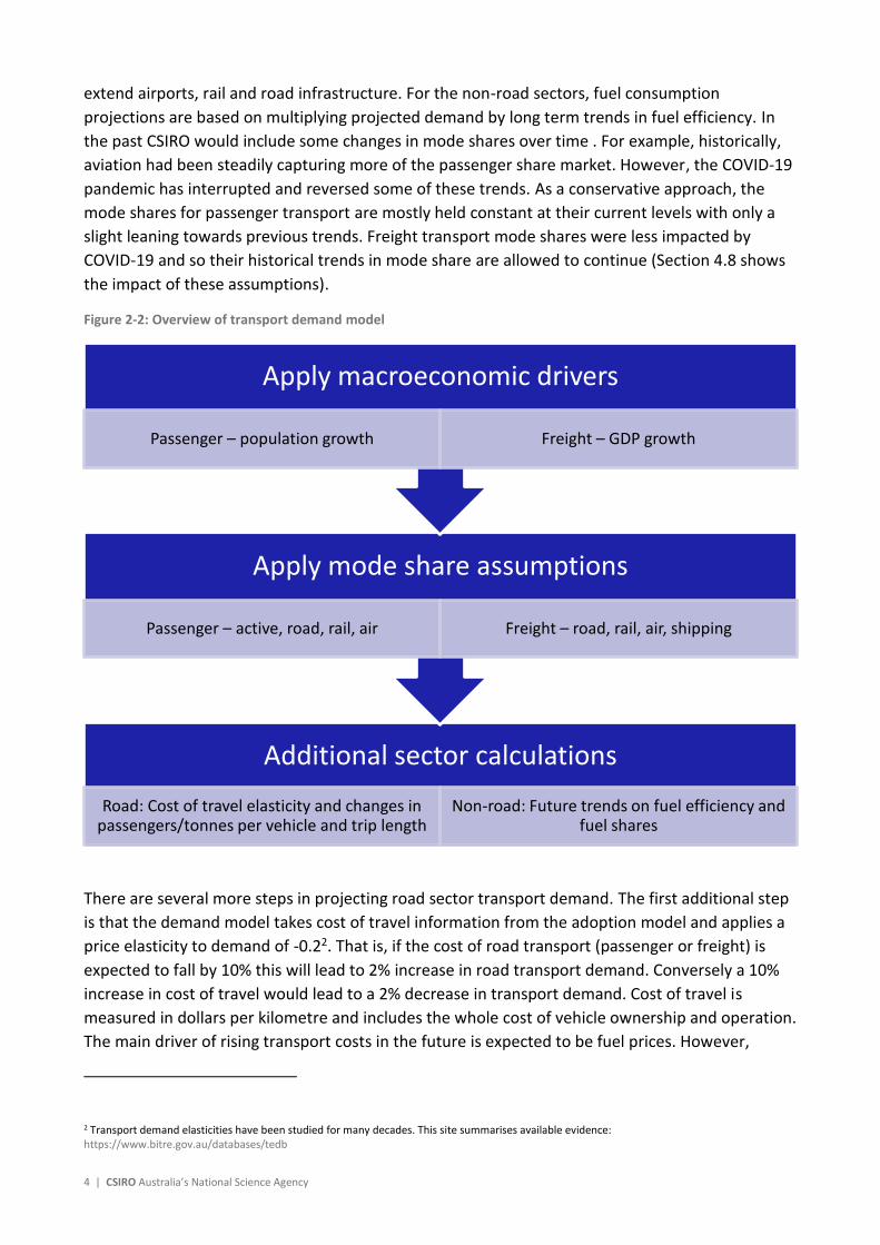
Payback periods are relatively straightforward to calculate and when compared to price also
captures the opportunity cost of staying with the technology substitute. The formula for the
payback period, expressed in years, is expressed as follows:
𝑃𝑎𝑦𝑏𝑎𝑐𝑘𝑃𝑒𝑟𝑖𝑜𝑑𝑣,𝑚,𝑠,𝑡 =𝐶𝑎𝑝𝑖𝑡𝑎𝑙𝑐𝑜𝑠𝑡𝑣,𝑚,𝑠,𝑡 − 𝐶𝑎𝑝𝑖𝑡𝑎𝑙𝐶𝑜𝑠𝑡𝐼𝐶𝐸𝑚,𝑡
𝐴𝑛𝑛𝑢𝑎𝑙𝑂𝑝𝑒𝑟𝑎𝑡𝑖𝑛𝑔𝐶𝑜𝑠𝑡𝐼𝐶𝐸𝑟,𝑚,𝑡 − 𝐴𝑛𝑛𝑢𝑎𝑙𝑂𝑝𝑒𝑟𝑎𝑡𝑖𝑛𝑔𝐶𝑜𝑠𝑡𝑟,𝑣,𝑚,𝑠,𝑡
Where:
𝐴𝑛𝑛𝑢𝑎𝑙𝑂𝑝𝑒𝑟𝑎𝑡𝑖𝑛𝑔𝐶𝑜𝑠𝑡𝑟,𝑣,𝑚,𝑠,𝑡
= 𝐴𝑛𝑛𝑢𝑎𝑙𝐹𝑢𝑒𝑙𝐶𝑜𝑠𝑡𝑣,𝑚,𝑠,𝑡 + 𝐴𝑛𝑛𝑢𝑎𝑙𝑀𝑎𝑖𝑛𝑡𝑒𝑛𝑎𝑛𝑐𝑒𝐶𝑜𝑠𝑡𝑣,𝑚
+ 𝐴𝑛𝑛𝑢𝑎𝑙𝑅𝑒𝑔𝑖𝑠𝑡𝑟𝑎𝑡𝑖𝑜𝑛𝐶𝑜𝑠𝑡𝑟,𝑣,𝑚 + 𝐴𝑛𝑛𝑢𝑎𝑙𝐼𝑛𝑠𝑢𝑟𝑎𝑛𝑐𝑒𝐶𝑜𝑠𝑡𝑟,𝑣,𝑚,𝑠,𝑡
𝐴𝑛𝑛𝑢𝑎𝑙𝑂𝑝𝑒𝑟𝑎𝑡𝑖𝑛𝑔𝐶𝑜𝑠𝑡𝐼𝐶𝐸𝑟,𝑚,𝑡
= 𝐴𝑛𝑛𝑢𝑎𝑙𝐹𝑢𝑒𝑙𝐶𝑜𝑠𝑡𝐼𝐶𝐸𝑚,𝑡 + 𝐴𝑛𝑛𝑢𝑎𝑙𝑀𝑎𝑖𝑛𝑡𝑒𝑛𝑎𝑛𝑐𝑒𝐶𝑜𝑠𝑡𝐼𝐶𝐸𝑚
+ 𝐴𝑛𝑛𝑢𝑎𝑙𝑅𝑒𝑔𝑖𝑠𝑡𝑟𝑎𝑡𝑖𝑜𝑛𝐶𝑜𝑠𝑡𝐼𝐶𝐸𝑟,𝑚 + 𝐴𝑛𝑛𝑢𝑎𝑙𝐼𝑛𝑠𝑢𝑟𝑎𝑛𝑐𝑒𝐶𝑜𝑠𝑡𝐼𝐶𝐸𝑟,𝑚,𝑡
r is the region
v is the five electric vehicle type: battery electric (short and long range), plug-in hybrid, fuel cell,
m is the ten road modes or vehicle types: passenger (3 sizes) , light commercial vehicle (3 sizes),
rigid truck, articulated truck, bus,
s is the five scenarios,
t is the financial year (to 2051-52).
The CapitalCost for internal combustion vehicles (ICE) varies by mode and time. The CapitalCost
for electric vehicles also varies by the vehicle type and scenario and is net of any subsidies.
The AnnualFuelCost for ICE vehicles is calculated as the petroleum price multiplied by average new
vehicle fuel efficiency and kilometres travelled per year. The assumptions for these factors change
by mode and over time. The AnnualFuelCost for electric vehicles is the same formula but varies by
vehicle type and scenario to recognise the use of different fuels (electricity and hydrogen) and
changes in electricity prices between scenarios.
A more difficult task than calculating the payback period is to identity the set of non-price
demographic or other factors that are required to capture other reasons that influences the
maximum market share assumption. CSIRO previously investigated the important non-price
factors and validated the approach of combining payback periods and non-price factors that
provides good locational predictive power for rooftop solar and electric vehicles (Higgins et al
2014; Higgins et al 2012).
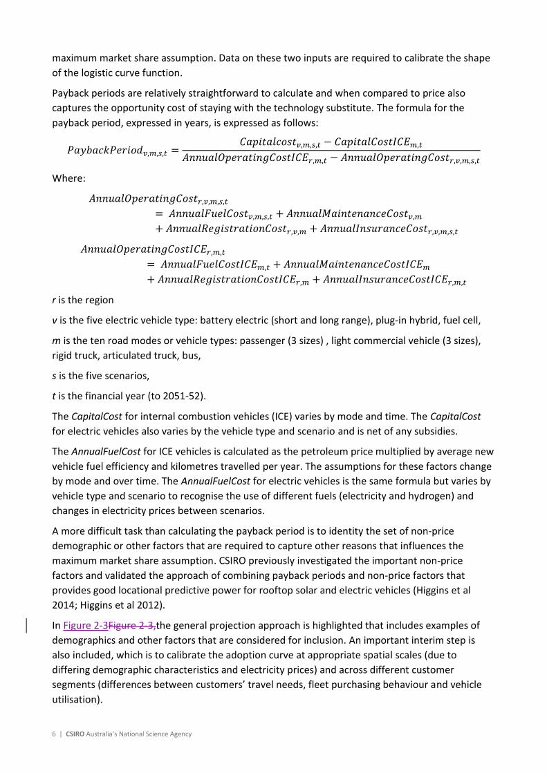
In Figure 2-3Figure 2-3,the general projection approach is highlighted that includes examples of
demographics and other factors that are considered for inclusion. An important interim step is
also included, which is to calibrate the adoption curve at appropriate spatial scales (due to
differing demographic characteristics and electricity prices) and across different customer
segments (differences between customers’ travel needs, fleet purchasing behaviour and vehicle
utilisation).

Electric vehicle projections 2021 | 7
Once the adoption curve is calibrated for all the relevant factors, the rate of adoption is evolved
over time by altering the inputs according to the outlined scenario assumptions4. For example,
differences in technology costs and prices between scenarios will alter the payback period and
lead to a different position on the adoption curve. Non-price scenario assumptions such as
available charging infrastructure or highest educational attainment in a region will result in
different adoption curve shapes (particularly the height at saturation or maximum market share).
Data on existing market shares determines the starting point on the adoption curve.
Figure 2-3 Adoption model methodology overview
The methodology also takes account of the total size of the available market and this can differ
between scenarios. For example, the total vehicle fleet requirement is relevant for electric
vehicles, while the number of customer connections is relevant for rooftop solar and battery
storage. The size of these markets is influenced by population growth, economic growth and
transport mode trends and this is discussed further in the scenario assumptions section. While a
maximum market share is set for the adoption curve based on various non-financial constraints,
maximum market share is only reached if the payback period falls. The applied maximum market
share assumptions are outlined in the Data Assumptions section.
All calculations are carried out at the Australian Bureau of Statistics Statistical Area Level 2 (SA2)
allowing the forecasts to align to the available demographic data. This also allows the conversion
of the data back to postcodes for aggregation to the state level as required. The Australian Bureau
of Statistics publishes correspondence files which provide conversion factors for moving between
4 Note that to “join” the short- and long-term projection models the trends projected to 2021-22 are seen as historical fact from the perspective of the long-term projection model and as such calibrate the adoption curve from that point.
Calculations
Key inputs Existing and new electricity load
Technology cost and electricity
tariffAge
Type/ownership of building
Educational attainment
Discretional income
Payback period Non-price factors
Multiple representative customer loads; Vehicle types and utilization rates ; ABS spatial categoriesSegmentation
Technology adoption curve calibration
Customer/ market growth
Existing and retiring capacity
Sales and market size
Customer / fleet model
t
%

8 | CSIRO Australia’s National Science Agency
commonly used spatial disaggregation. Each spatial disaggregation can also be associated with a
state for aggregation purposes.
2.1.4 Commercial vehicles
It may be argued that commercial vehicle purchasers would be more weighted to making their
decisions on financial grounds only. That is, commercial vehicle sales would rapidly accelerate
towards electric vehicles as soon as the whole of life cost of owning an EV falls (which also occurs
sooner than for residential owners because of the longer average driving distances of commercial
vehicles). However, it is assumed that infrastructure constraints including the split incentives or
landlord-renter problem which can be captured using adoption curves are also relevant for
businesses noting that many commercial vehicles park at residential premises. For business parked
vehicles, if the business does not own the building, installing charging infrastructure may not be
straight-forward. Hence, the applicability of vehicle range to a business's needs is just as relevant
as whether vehicle range will suit a household's needs.
2.2 Demographic factors and weights
The projection methodology includes selecting a set of non-price factors, typically drawn from
accessible demographic data to calibrate the consumer technology adoption curve in each SA2
region. CSIRO assigns different weights to each factor to reflect their relative importance. The next
section outlines the factors and weights chosen for electric vehicles.
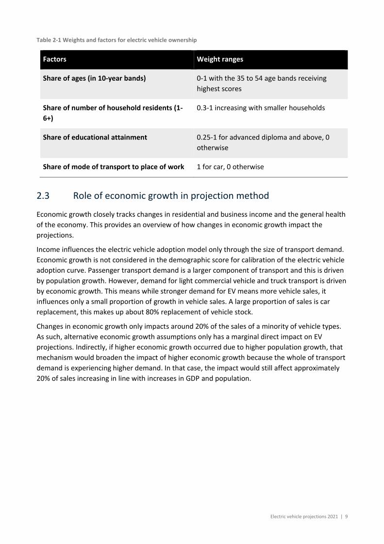
2.2.1 Weights and factors for electric vehicles
Previous analysis by Higgins et al (2012) validated several demographic factors and weights for
Victoria. A similar combination of factors and weights is applied and outlined in Table 2-1. These
weighting factors provide a guide for the adoption locations, particularly during the early adoption
phase which Australia currently remains in. However, adoption is allowed to grow in all locations
over time. It is likely that some of the factors included act as a proxy for other drivers not explicitly
included (such as income).
The weights and factors are used to calculate a score for each SA2 region to indicate relative
propensity for electric vehicle uptake. After a general level of maximum national electric vehicle
adoption is set, for example 50%, the SA2 weights and factors are used to score to adjust the local
level of adoption up or down by a maximum of plus or minus 25%. In this case the best scoring SA2
region achieves a maximum adoption of 75% and the worst scoring region 25%. The maximum
national electric vehicle adoption assumptions are outlined in Section 4 Table 4-4.
Electric vehicle projections 2021 | 9
Table 2-1 Weights and factors for electric vehicle ownership
Factors Weight ranges
Share of ages (in 10-year bands) 0-1 with the 35 to 54 age bands receiving
highest scores
Share of number of household residents (1-
6+)
0.3-1 increasing with smaller households
Share of educational attainment 0.25-1 for advanced diploma and above, 0
otherwise
Share of mode of transport to place of work 1 for car, 0 otherwise
2.3 Role of economic growth in projection method
Economic growth closely tracks changes in residential and business income and the general health
of the economy. This provides an overview of how changes in economic growth impact the
projections.
Income influences the electric vehicle adoption model only through the size of transport demand.
Economic growth is not considered in the demographic score for calibration of the electric vehicle
adoption curve. Passenger transport demand is a larger component of transport and this is driven
by population growth. However, demand for light commercial vehicle and truck transport is driven
by economic growth. This means while stronger demand for EV means more vehicle sales, it
influences only a small proportion of growth in vehicle sales. A large proportion of sales is car
replacement, this makes up about 80% replacement of vehicle stock.
Changes in economic growth only impacts around 20% of the sales of a minority of vehicle types.
As such, alternative economic growth assumptions only has a marginal direct impact on EV
projections. Indirectly, if higher economic growth occurred due to higher population growth, that
mechanism would broaden the impact of higher economic growth because the whole of transport
demand is experiencing higher demand. In that case, the impact would still affect approximately
20% of sales increasing in line with increases in GDP and population.
10 | CSIRO Australia’s National Science Agency
3 Scenario definitions
The five scenarios are Current Trajectory, Slow Growth, Net Zero, Sustainable Growth and Export
Superpower. Rapid Decarbonisation is a sensitivity of Export Superpower. The AEMO scenario
definitions are provided as short narratives and settings for key drivers in Table 3-1. For the
electric vehicles projections, this section provides an extended scenario definition table based on a
deeper consideration of the economic, infrastructure and policy drivers. The section then
describes each of the financial and non-financial drivers in more detail.
Current Trajectory scenario
The Current Trajectory scenario reflects a future energy system based around current government
policies and best estimates of all key drivers. This scenario represents the current transition of the
energy industry under current policy settings and technology trajectories, where the transition
from fossil fuels to renewable generation is generally led by market forces. Uptake of DER, energy
efficiency measures and the electrification of the transport sector proceeds in line with AEMO’s
current best estimates. The relevant purpose for this scenario is:
• To provide a basis on which to assess the development of the system under currently funded
and/or legislated policies and commitments, using the most probable value/best estimate for
each input.
Net Zero scenario
This reflects a world that is like Current Trajectory in the first decade but with a shift in policy
towards achieving Net Zero emissions economy wide by 2050.
Sustainable Growth scenario
Higher decarbonisation ambitions are supported by rapidly falling costs for battery storage and
variable renewable energy (VRE), which drive consumers’ actions and higher levels of
electrification of other sectors. Economic and population growth are similar to Current Trajectory.
The main differences to Current Trajectory are:
• Economy wide Net Zero emissions by 2050
• Increased cost-competitiveness of VRE and batteries relative to fossil fuel generation.
• DER uptake is driven by consumers seeking to take a greater degree of ownership over their
consumption, choosing when and how to consume energy. This is also aided by continued
technological advances that extend the strong uptake in DER technologies. Participation in
virtual power plant (VPP) aggregation schemes is higher.
• There are high levels of electrification of transport and energy efficiency
The relevant purposes for this scenario are:
• To understand the impact of strong decarbonisation and DER uptake on the needs of the
electricity system, and in particular to explore the potential risk of under-investment in the
infrastructure required to facilitate this transition.

Electric vehicle projections 2021 | 11
• To explore the system security impact of high penetration of DER and potential issues and
challenges in distribution and transmission networks, and what investments could address
these.
Slow Growth scenario
This scenario includes the lowest level of economic growth following the global COVID-19
pandemic, which increases the likelihood of industrial load closures. Decarbonisation at a policy
level takes a back seat, but strong uptake of distributed PV continues, particularly in the short-
term in response to a number of incentives.
• The rate of technological development and cost reductions stagnates, as falling private
investment reduces the speed of cost reductions in technologies such as battery storage.
• In search of cost savings and in response to low interest rates and government incentives to aid
the recovery from COVID-19, consumers continue to install distributed PV at high rates,
continuing the trends observed during 2020, where uptake has held up and in many regions
increased, despite adverse economic conditions. Over time these impacts dissipate and
distributed PV uptake moderates.
Key differences to the Current Trajectory scenario include:
• Lower levels of decarbonisation ambitions both internationally and domestically.
• Very low economic activity and population growth.
• Lower levels of electrification.
• Stronger level of DER uptake in the near term
The relevant purposes for this scenario for these consulting services are:
• To assess the risk of over-investment in the power system, in a future where operational
demand is much lower, and some less certain policy drivers do not proceed.
• To explore operational and system security risks associated with falling levels of minimum
demand
Export Superpower scenario
This scenario represents a world with very high levels of electrification and hydrogen production,
fuelled by strong decarbonisation targets and leading to strong economic growth. Key differences
to the Current Trajectory scenario include:
• Economy wide Net Zero emission by early 2040s
• The highest level of international decarbonisation ambition, consistent with a target of limiting
the global temperature rise to 1.5⁰C by 2100 over pre-industrial levels – this also results in the
strongest decarbonisation requirement in the NEM across the scenarios.
• Stronger economic activity and higher population growth.
• Continued improvements in the economics of hydrogen production technologies that enable the
development of a large NEM connected hydrogen production industry in Australia for both
export and domestic consumption.

12 | CSIRO Australia’s National Science Agency
• Higher levels of electrification across many sectors, with strong light vehicle electrification but
fewer large electric trucks due to competition from hydrogen fuel-cell trucks.
The relevant purpose for this scenario for these consulting services is:
• To understand the implications and needs of the power system under conditions that result in
the development of a renewable generation export economy which significantly increases grid
consumption and necessitates developments in significant regional renewable energy
generation.
• To assess the impact, and potential benefits, of large amounts of flexible electrolyser load.
Rapid Decarbonisation sensitivity
The Rapid Decarbonisation sensitivity has the same scenario settings as Export Superpower but
without a large NEM connected hydrogen industry.
Table 3-1 AEMO scenario definitions
Scenario/sensitivity SLOW GROWTH
CURRENT TRAJECTORY
NET ZERO SUSTAINABLE GROWTH
RAPID DECARBONISATION
EXPORT SUPERPOWER
Economic growth and population outlook*
Low Moderate Moderate Moderate High High
Energy efficiency improvement
Low Moderate Moderate High High High
DSP Low Moderate Moderate High High High
Distributed PV (per capita uptake tendency)
Moderate, but elevated in the short term
Moderate Moderate High High High
Battery storage installed capacity
Low Moderate Moderate High High High
Battery storage aggregation / VPP deployment by 2050
Low Moderate Moderate High High High
Battery Electric Vehicle (BEV) uptake
Low Moderate Moderate High High High*
BEV charging time switch to coordinated dynamic charging by 2030
Low Moderate Moderate High High Moderate/High
Electrification of other sectors
Low Low/Moderate Moderate Moderate/High High Moderate/High
Hydrogen uptake Minimal Minimal Minimal Minimal Minimal
Large NEM-connected export and domestic consumption
Shared Socioeconomic SSP3 SSP2 SSP2 SSP1 SSP1 SSP1
Pathway (SSP)
International Energy Agency (IEA) 2020 World Energy Outlook (WEO) scenario
Delayed Recovery Scenario (DRS)
Stated Policy Scenario (STEPS)
Stated Policy Scenario (STEPS)
Sustainable Development Scenario (SDS)
Net Zero Emissions by 2050 case (NZE2050)
Net Zero Emissions by 2050 case (NZE2050)
Representative Concentration Pathway (RCP) (mean
RCP7.0 (~4°C)
RCP4.5 (~2.6°C)
RCP4.5 (~2.6°C)
RCP2.6 (~1.8°C)
RCP1.9 (<1.5°C) RCP1.9 (<1.5°C)

Electric vehicle projections 2021 | 13
Scenario/sensitivity SLOW GROWTH
CURRENT TRAJECTORY
NET ZERO SUSTAINABLE GROWTH
RAPID DECARBONISATION
EXPORT SUPERPOWER
temperature rise by 2100)
Decarbonisation target
26-28% reduction by 2030.
26-28% reduction by 2030.
26-28% reduction by 2030
Consistent with limiting temperature rise to 2 degrees.
Consistent with limiting temperature rise to 1.5 degrees.
Consistent with limiting temperature rise to 1.5 degrees.
Economy-wide Net Zero target by 2050.
Economy-wide before 2050
Economy-wide Net Zero by early 2040s
Economy-wide Net Zero by early 2040s
Generator and storage build costs
CSIRO GenCost Central
CSIRO GenCost Central
CSIRO GenCost Central
CSIRO GenCost High VRE
CSIRO GenCost High VRE
CSIRO GenCost High VRE
Generator retirements
In line with expected closure years, or earlier if economic to do so.
In line with expected closure years, or earlier if economic.
In line with expected closure years, or earlier if economic or driven by decarbonisation objectives beyond 2030.
In line with expected closure year, or earlier if economic or driven by decarbonisation objectives
In line with expected closure year, or earlier if economic or driven by decarbonisation objectives
In line with expected closure year, or earlier if economic or driven by decarbonisation objectives
Relative project finance costs
Lower than Central, reflecting lower rates of return with lower economic growth
In line with current long-term financing costs appropriate for a private enterprise
In line with current long-term financing costs appropriate for a private enterprise
As per Central As per Central As per Central
3.1.1 Extended scenario definitions
The AEMO scenario definitions have been extended in Table 3-2 by adding additional detail on the
economic, infrastructure and business model drivers. The purpose is to fill out more detail about
how the scenarios are implemented whilst remaining consistent with the higher level AEMO
scenario definitions. The scenario definitions are in some cases described here in general terms
such as “High” or “Low”. More specific scenario data assumptions are outlined further in the next
section and in Section 4.

14 | CSIRO Australia’s National Science Agency
Table 3-2 Extended scenario definitions
Driver Slow
Growth
Current
Trajectory Net Zero
Sustainable
Growth
Export
Superpower
Rapid
Decarbonisa
tion
Economic
Timing of cost1 parity
of short-range electric
vehicles with ICE
2035 2030 2030 2025 2025 2025
Cost of fuel cell
vehicles
High Medium Medium Medium Low Medium
Infrastructure
Growth in apartment
share of dwellings
High Medium Medium Medium Low Low
Decline in home
ownership
High Medium Medium Medium Low Low
Extent of access to
variety of charging
options
Low Medium Medium
High post
2030
High High High
Business model
Feasibility of ride
sharing services
Low Medium Medium High High High
Affordable public
charging availability
Low Medium Medium
High post
2030
High High High
Vehicle to home or
grid (passenger
vehicles)
Yes from
2030
Yes from
2030
Yes from
2030
Yes from
2030
Yes from
2030
Yes from
2030
1. Upfront sales costs of vehicle, not whole of vehicle running cost. Short range is less than 300km.
3.2 Financial and non-financial scenario drivers
3.2.1 Direct economic drivers
For privately owned electric and fuel cell vehicles the economic drivers and the approach to
including them in the scenarios is listed in Table 3-3.
Future hydrogen fuel costs are hard to predict because there is a diversity of possible supply
chains, each with their own unique cost structures. While natural gas based hydrogen is currently
lowest cost, by the time fuel cell electric vehicles (FCEVs) are relevant, electrolysis hydrogen

Electric vehicle projections 2021 | 15
production is likely to be more competitive and offers the most flexibility for accessing a low
carbon energy source and allowing hydrogen to be generated at either the end-user’s location, at
fuelling stations or at dedicated centralised facilities.
Table 3-3: Economic drivers of electric and fuel cell electric vehicles (FCEV) and approach to including them in
scenarios
Driver Approach to including in scenarios
The whole cost of driving an electric or fuel
cell vehicle including vehicle, retail electricity,
the charging terminal (wherever it is
installed), hydrogen fuel, insurance,
registration and maintenance costs
Vehicle costs vary by scenario and are outlined
in Section 4.1.1. Retail electricity prices are
varied by scenario and outlined in Section
4.2.1. The remaining factors are held constant.
The whole cost of driving an internal
combustion engine (ICE) vehicle as an
alternative including vehicle, fuel, insurance,
registration and maintenance costs
Not varied by scenario
Perceptions of future changes in petroleum-
derived fuel costs including global oil price
volatility and any fuel excise changes
Not varied by scenario
The structure of retail electricity prices
relating to electric vehicle recharging
Varied by scenario and outlined in 4.7
The perceived vehicle resale value Not varied by scenario
For autonomous private and ride share vehicles the additional economic drivers compared to
electric and fuel cell vehicles and the approach to including them in scenarios is shown in Table
3-4.

16 | CSIRO Australia’s National Science Agency
Table 3-4: Economic drivers of autonomous private and ride share vehicles and approach to including them in
scenarios
Driver Approach to including in scenarios
The cost of the autonomous driving capability On-cost of autonomous features not varied by
scenario but underlying cost of electric vehicle
carried by scenario as outlined in Section 4.1.1
The value of avoided driving time Not varied by scenario but assumptions
discussed in Section 4.1.2
The lower cost of travel from higher
utilisation of the ride-share vehicle compared
to privately owned vehicles (accounting for
some increased trip lengths to join up the
routes of multiple passengers)
Not varied by scenario
The avoided cost of wages to the transport
company for removing drivers from
autonomous trucks
Not varied by scenario but assumptions
discussed in Section 4.1.2
Higher utilisation and fuel efficiency
associated with autonomous trucks
Not varied by scenario
3.2.2 Infrastructure drivers
The are several infrastructure barriers to accessing electric vehicles and associated refuelling
(Table 3-5). Electric, fuel cell and autonomous ride share vehicles all face the common constraint
of a lack of variety of models in the initial phases of supply of those vehicles. While perhaps ride
share vehicles can be more generically designed for people moving, purchasers of privately owned
vehicles will prefer access to a wider variety of models to meet their needs for the how they use
their car (including sport, sedan, SUV, people moving, compact, medium, large, utility, 4WD,
towing).

Electric vehicle projections 2021 | 17
Table 3-5: Infrastructure drivers for electric and fuel cell vehicles and approach to including them in scenarios
Driver Approach to including in scenarios
Convenient location for a power point or dedicated
charging terminal in the home garage or a frequently
used daytime parking area for passenger vehicles
and at parking or loading areas for business vehicles
such as light commercial vehicles, trucks and buses
Varied by scenario and expressed as
maximum market share in Section 4.5
Whether the residence or business has ownership or
other extended tenancy of the building or site and
intention to stay at that location to get a long-term
payoff from the upfront costs of installing the
charger.
Varied by scenario and expressed as
maximum market share in Section 4.5
Convenient access to highway recharging for owners
without access to extended range capability (or
other options, see below)
Varied by scenario and expressed as
maximum market share in Section 4.5
Access to different engine configurations of electric
vehicles (e.g. fully electric short range, fully electric
long range and plug-in hybrid electric and internal
combustion)
Varied by scenario and expressed as
maximum market share in Section 4.5
Convenient access to other means of transport such
as a second car in the household, ride sharing, train
station, airport and hire vehicles for longer range
journeys
Varied by scenario and expressed as
maximum market share in Section 4.5
Whether hydrogen distribution and refuelling
terminals have been deployed widely enough for
convenient use of fuel cell vehicles
Varied by scenario and expressed as
maximum market share in Section 4.5
Key infrastructure drivers for FCEVs are varied by scenario as maximum market share assumptions
and outlined in Section 4.5. The drivers are:
• A mature hydrogen production and distribution supply chain for FCEVs. There are many
possible production technologies and resources and many ways hydrogen can be
distributed with scale being a strong determinant of the most efficient distribution
pathway (e.g. trucks at low volumes, pipelines at high volumes).
• The greater availability of FCEVs for sale.
Sufficient electricity distribution network capacity to meet coincident charging requirements of
high electric vehicle share could also be an infrastructure constraint if not well planned for.
However, networks are obligated to expand capacity or secure demand management services to
18 | CSIRO Australia’s National Science Agency
meet load where needed and so any such constraints would only be temporary. If hydrogen supply
is based on electrolysis this will also mean increased requirements for electricity infrastructure,
but its location depends on whether the electrolysis is on site (e.g. at a service station) or
centralised (where the location might be a prospective renewable energy zone or fossil fuel
resource).
Given the constraints of commute times and cost of land in large cities, there is a slow trend
towards apartments rather than separate dwellings in the capital and large cities where most
Australians live. This is expected to result in a lower share of customers with access to their own
roof or garage space impacting all types of embedded generation (these assumptions are defined
later in the report). There has also been recent evidence of a fall in home ownership, especially
amongst younger age groups. For electric vehicles these trends might also work towards lower
adoption as denser cities tend to encourage greater uptake of non-passenger car transport
options and ride sharing services (discussed further in the next section) which result in fewer
vehicles sold. Home ownership and separate dwelling share are varied by scenario and outlined in
Section 4.4
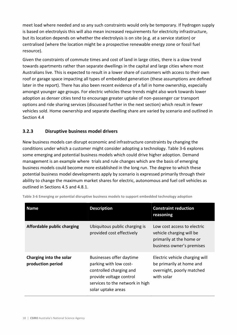
3.2.3 Disruptive business model drivers
New business models can disrupt economic and infrastructure constraints by changing the
conditions under which a customer might consider adopting a technology. Table 3-6 explores
some emerging and potential business models which could drive higher adoption. Demand
management is an example where trials and rule changes which are the basis of emerging
business models could become more established in the long run. The degree to which these
potential business model developments apply by scenario is expressed primarily through their
ability to change the maximum market shares for electric, autonomous and fuel cell vehicles as
outlined in Sections 4.5 and 4.8.1.
Table 3-6 Emerging or potential disruptive business models to support embedded technology adoption
Name Description Constraint reduction
reasoning
Affordable public charging Ubiquitous public charging is
provided cost effectively
Low cost access to electric
vehicle charging will be
primarily at the home or
business owner’s premises
Charging into the solar
production period
Businesses offer daytime
parking with low cost-
controlled charging and
provide voltage control
services to the network in high
solar uptake areas
Electric vehicle charging will
be primarily at home and
overnight, poorly matched
with solar
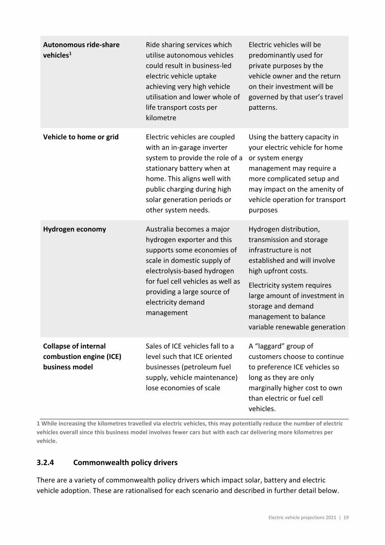
Electric vehicle projections 2021 | 19
Autonomous ride-share
vehicles1
Ride sharing services which
utilise autonomous vehicles
could result in business-led
electric vehicle uptake
achieving very high vehicle
utilisation and lower whole of
life transport costs per
kilometre
Electric vehicles will be
predominantly used for
private purposes by the
vehicle owner and the return
on their investment will be
governed by that user’s travel
patterns.
Vehicle to home or grid Electric vehicles are coupled
with an in-garage inverter
system to provide the role of a
stationary battery when at
home. This aligns well with
public charging during high
solar generation periods or
other system needs.
Using the battery capacity in
your electric vehicle for home
or system energy
management may require a
more complicated setup and
may impact on the amenity of
vehicle operation for transport
purposes
Hydrogen economy Australia becomes a major
hydrogen exporter and this
supports some economies of
scale in domestic supply of
electrolysis-based hydrogen
for fuel cell vehicles as well as
providing a large source of
electricity demand
management
Hydrogen distribution,
transmission and storage
infrastructure is not
established and will involve
high upfront costs.
Electricity system requires
large amount of investment in
storage and demand
management to balance
variable renewable generation
Collapse of internal
combustion engine (ICE)
business model
Sales of ICE vehicles fall to a
level such that ICE oriented
businesses (petroleum fuel
supply, vehicle maintenance)
lose economies of scale
A “laggard” group of
customers choose to continue
to preference ICE vehicles so
long as they are only
marginally higher cost to own
than electric or fuel cell
vehicles.
1 While increasing the kilometres travelled via electric vehicles, this may potentially reduce the number of electric
vehicles overall since this business model involves fewer cars but with each car delivering more kilometres per
vehicle.
3.2.4 Commonwealth policy drivers
There are a variety of commonwealth policy drivers which impact solar, battery and electric
vehicle adoption. These are rationalised for each scenario and described in further detail below.

20 | CSIRO Australia’s National Science Agency
Emissions Reduction Fund5 and Climate Solutions Fund
The ERF consists of several methods for emission reduction under which projects may be eligible
to claim emission reduction and bid for Australian Carbon Credit Units (ACCUs) which are currently
awarded via auction at around $15/tCO2e. The relevant method in this case is the Carbon Credits
(Carbon Farming Initiative – Land and Sea Transport) Methodology Determination 2015. It is
possible for businesses to develop projects under the ERF where each project may receive funding
for deployment of electric vehicles. However, there have been no significant uptake of this scheme
as the incentive is not significant. Although it is expected for the ACCU price to increase over time,
it currently provides an incentive of only $15/tCO2e. ICE passenger vehicle emissions is around 4
tonnes per year and this is only estimated to be roughly $60 per year in benefits.
Potential changes to Commonwealth renewable energy and climate policy
While there are currently no announced changes to renewable energy and climate policy, given
Australia’s nationally determined commitment at the Paris UNFCCC meeting, it is likely there may
be adjustments to those policies in the future. The Export Superpower and Sustainable Growth
scenarios imply the deployment of such additional policies. Given the low cost of greenhouse gas
emissions as a share of the overall cost of transport, it is more likely that a non-price mechanism
will be deployed in the transport sector to achieve emission reduction.
Australia is one of the few developed countries internationally without vehicle greenhouse gas
emissions or fuel economy standards. Consequently, vehicles sold in Australia are around 20% less
efficient than the same model sold in the UK (CCA 2014). Low emission vehicles such as electric
vehicles are expected to be adopted with or without emission standards, but new policies could
accelerate their adoption to ensure any Net Zero emission targets are met in a timely manner
(without the delay imposed by stock turnover rates). In addition, there is also currently no
Commonwealth fuel excise on electricity or hydrogen used in transport. Some states have begun
considering or introducing kilometre based electric vehicle charges. As such, CSIRO has included
state based road user charges into the modelling that is outlined in the next section.
3.2.5 State policy drivers
South Australia and Victoria have both announced new road user chargers for electric vehicles
which are otherwise exempt from fuel excise6. Other states may also be considering introducing
similar policies7. The rate of the road user charge is yet to be determined in South Australia but for
Victoria, it is 2.5 cents/km. The average driving kilometres of approximately 11,000 km/year would
represent an annual charge of $275.
5 The Emissions Reduction Fund (ERF) was extended by the Climate Solutions Fund announced in 2019
6 While policy announcements raise this point, it is not clear how one substitutes for the other in practice when fuel excise is collected by the commonwealth and road user charges are proposed to be collected by states.
7 It has been reported that the Board of Treasurers commissioned research on how to introduce road user charges: Australian states were warned road user tax on electric vehicles could discourage uptake | Electric, hybrid and low-emission cars | The Guardian
Electric vehicle projections 2021 | 21
South Australia has an $18 million EV action plan8 which includes building a fast charging network
and purchase of electric vehicles for its government fleet. This has strong similarities to Western
Australia9 which has committed $21 million to creating a fast charging network covering from
Perth to Esperance in the south, Kalgoorlie in the east and Kununurra in the north. It will also
acquire 25 electric vehicles for the state government fleet.
Victoria provides a $100 discount on annual registration fees for electric vehicles10. This represents
an ongoing subsidy of electric vehicles relative to other vehicle types. Other states offer similar
policies including stamp duty discounts. The Victorian government has also announced a target of
50% of light vehicle sales to be zero emission vehicles (i.e. including both battery and fuel cell
electric vehicles)11. The target is supported by subsidies for 20,000 vehicles available from July
2021. The first 4,000 vehicles will receive a subsidy of $3,000 with the amount of subsidy for the
remainder yet to be determined. Due to the timing of this policy announcement, this has not been
included in the modelling and may accelerate adoption of both battery and fuel cell electric
vehicles in Victoria.
The Australian Capital Territory’s policy12 offers a substantial package of financial incentives.
Interest free loans of up to $15,000 are available as well as stamp duty and registration
exemptions. Average environmental performance vehicles at or below $45,000 are normally
subject to 3% stamp duty. A 5% stamp duty is applicable for each dollar above $45,000. Electric
vehicles registered for the first time are exempt from this stamp duty. This application of different
stamp duty rates to new vehicles is an approach unique to the Australian Capital Territory. It
amounts to an upfront subsidy of $1350 on a $45,000 electric vehicle or $2110 on a $60,000
electric vehicle. Electric vehicles receive 2 years of free vehicle registration.
Given these policy developments at the Commonwealth and state level, the policies applied are
outlined in Table 3-7 and assigned to each scenario.
8 State Government’s Electric Vehicle Action Plan | LGA South Australia
9 Electric Vehicle Strategy | Western Australian Government (www.wa.gov.au)
10 Hybrid or electric vehicle registration discounts : VicRoads
11 Zero Emissions Vehicle (ZEV) Subsidy | Solar Victoria
12 Zero Emissions Vehicles - Environment, Planning and Sustainable Development Directorate - Environment (act.gov.au)

22 | CSIRO Australia’s National Science Agency
Table 3-7 Electric vehicle policy settings by scenario
Slow Growth Current Trajectory
Net Zero Sustainable Growth
Export Superpower
Rapid Decarbonisation
ICE vehicle availability
New ICE vehicles unavailable beyond 2070
New ICE vehicles unavailable beyond 2060
New vehicles unavailable beyond 2050
New vehicles unavailable beyond 2040
New vehicles unavailable beyond 2035
New vehicles unavailable beyond 2035
ICE retirement
Natural retirement
Natural retirement
Deregistered from 2055
Deregistered from 2050
Deregistered from 2045
Deregistered from 2045
Road user charges
2.5c/km from 2022
2.5c/km from 2025
2.5c/km from 2025
2.5c/km from 2030
2.5c/km from 2035
2.5c/km from 2035
Subsidies (stamp duty, registration exemptions or direct financing)
Current policies retained until 2025
Current policies retained until 2030
Current policies retained until 2030
Current policies retained until 2030
Current policies retained until 2030
Current policies retained until 2030

Electric vehicle projections 2021 | 23
4 Data assumptions
This section outlines the key data assumptions applied to implement the scenarios. Some
additional data assumptions which are used in all scenarios are described in Appendix A.
4.1 Technology costs
4.1.1 Electric and fuel cell vehicles
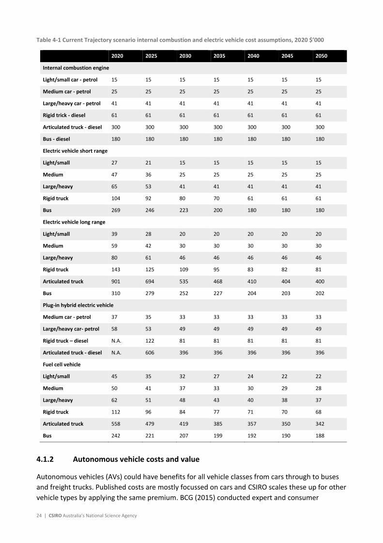
Current Trajectory scenario short-range electric vehicle (SREV) costs are assumed to reach upfront
cost of vehicle parity with internal combustion engine light vehicles in 2030 and remain at that
level thereafter (Table 4-1). Heavy SREVs are assumed to reach up front cost parity in 2040 due to
their delayed development relative to light vehicles and higher duty requirements (both load and
distance). Up front cost parity may be reached earlier in other countries where vehicle emissions
standards are expected to increase the cost of internal combustion vehicles over time. The
modelling considers SREV adoption across five vehicle classes: light, medium and large cars, rigid
trucks and buses. Long-range electric vehicles (LREVs) also include larger articulated trucks which
perform the bulk of long-distance road freight. LREVs do not reach up front vehicle cost parity
because their extra range adds around $5,000 in battery costs to light vehicles (and proportionally
more to heavy vehicles). However, from a total cost of driving perspective (i.e. $/km), LREVs are
below cost parity by 2030, paying back the additional upfront cost through fuel savings within 2-3
years.
The modelling does not consider applying a plug-in hybrid engine configuration to the small light
vehicle class as these vehicles are already efficient so the additional cost would be difficult to
payback with limited additional fuel savings.
The Slow Growth, Net Zero, Export Superpower, Sustainable Growth and Rapid Decarbonisation
assumptions are framed relative to these Current Trajectory scenario assumptions. The Net Zero
cost trajectories are the same as Current Trajectory. In the Slow Growth scenario, it is assumed
that the cost reductions are delayed by 5 years to 2035. In the Export Superpower, Rapid
Decarbonisation and Sustainable Growth scenarios it is assumed the cost reductions are brought
forward by 5 years to 2025.
Given that fuel cell and electric vehicles have significantly fewer parts than internal combustion
engines it could also have been reasonable to consider their costs reaching lower than parity with
internal combustion vehicles. However, in the context of the adoption projection methodology
applied here, when the upfront price of an electric vehicle equals the upfront price of an
equivalent internal combustion vehicle, the payback period is already zero in the sense that there
is no additional upfront cost to recover through fuel savings. After this point, adoption is largely
driven by non-financial considerations. Also, it was considered that vehicle manufacturers might
continue to offer other value-adding features to the vehicle if this point is reached rather than
continue reducing vehicle prices (e.g. luxury, information technology and sport features).
24 | CSIRO Australia’s National Science Agency
Table 4-1 Current Trajectory scenario internal combustion and electric vehicle cost assumptions, 2020 $’000
2020 2025 2030 2035 2040 2045 2050
Internal combustion engine
Light/small car - petrol 15 15 15 15 15 15 15
Medium car - petrol 25 25 25 25 25 25 25
Large/heavy car - petrol 41 41 41 41 41 41 41
Rigid trick - diesel 61 61 61 61 61 61 61
Articulated truck - diesel 300 300 300 300 300 300 300
Bus - diesel 180 180 180 180 180 180 180
Electric vehicle short range
Light/small 27 21 15 15 15 15 15
Medium 47 36 25 25 25 25 25
Large/heavy 65 53 41 41 41 41 41
Rigid truck 104 92 80 70 61 61 61
Bus 269 246 223 200 180 180 180
Electric vehicle long range
Light/small 39 28 20 20 20 20 20
Medium 59 42 30 30 30 30 30
Large/heavy 80 61 46 46 46 46 46
Rigid truck 143 125 109 95 83 82 81
Articulated truck 901 694 535 468 410 404 400
Bus 310 279 252 227 204 203 202
Plug-in hybrid electric vehicle
Medium car - petrol 37 35 33 33 33 33 33
Large/heavy car- petrol 58 53 49 49 49 49 49
Rigid truck – diesel N.A. 122 81 81 81 81 81
Articulated truck - diesel N.A. 606 396 396 396 396 396
Fuel cell vehicle
Light/small 45 35 32 27 24 22 22
Medium 50 41 37 33 30 29 28
Large/heavy 62 51 48 43 40 38 37
Rigid truck 112 96 84 77 71 70 68
Articulated truck 558 479 419 385 357 350 342
Bus 242 221 207 199 192 190 188
4.1.2 Autonomous vehicle costs and value
Autonomous vehicles (AVs) could have benefits for all vehicle classes from cars through to buses
and freight trucks. Published costs are mostly focussed on cars and CSIRO scales these up for other
vehicle types by applying the same premium. BCG (2015) conducted expert and consumer
Electric vehicle projections 2021 | 25
interviews establishing that an autonomous vehicle (AV) would have a premium of around
$15,000 and that customers would be willing to pay a premium of around $5000 to own a fully
autonomous road passenger vehicle. This last point seems to align well with the concept of valuing
people’s time saved in transport studies. If commuting via an autonomous vehicle gives back 1
hour of time for other activities per working day and if that time is valued that at around $20/hr
(slightly more than average earnings), then its value over 235 working days (assuming 5 weeks
leave) is $4700 per year.
KPMG (2018) uses a value of 20% for the AV cost premium which would be $3,000 to $8,200 for
the standard passenger vehicle types used in our modelling. CSIRO interprets this costing
approach as a focus on a larger vehicle and longer-term point of view (i.e. not a first of a kind
vehicle). This matches the expectation that the autonomous vehicles would initially be targeted
towards the larger less-budget conscious end of the market.
Based on these studies, CSIRO assumes AVs commands a premium starting at $10,000 in 2020
decreasing to $7,500 by 2030 and remaining at that level. Given how consumers value time,
significant cost reductions beyond these assumptions are not be necessary to support growth in
adoption. However, it is assumed that the vehicles will not be available for adoption until the late
2020s.
For freight vehicles, the major value from AVs are fuel consumption savings through platooning,
resting drivers so they can complete longer trips without a break or, if technically feasible,
completely removing the driver.
By removing the driver, the wages costs are avoided which are on average around $75,000 per
annum while also increasing truck utilisation. Our assumption is that AV truck premiums will be
significantly higher (proportionate to the ratio of truck to passenger car costs) owing to the
greater complications of a larger vehicle under load in terms of reaction times for autonomous
systems and the requirement of better sensing for AVs. However, if these vehicles can achieve full
autonomy, the financial incentives are significant.
These assumptions set the economic foundations for AVs which is an important driver for
adoption. The adoption of AVs, particularly those with ride share capability in the passenger
segment, results in changes to the required size of vehicle fleet and sales which has secondary
impacts on the adoption of all vehicles. These issues are discussed further in Section 4.8.1.
4.2 Electricity tariffs
4.2.1 Assumed trends in retail prices
Retail prices are stable throughout the projection period and are not a strong driver of uptake
trends or differences between scenarios. This is because electricity refuelling costs are a small
proportion of total vehicle running costs (the vehicle is the main cost). Modest differences
between a small component across scenarios therefore cannot drive major changes in vehicle
adoption.
Broadly speaking retail electricity generation prices are expected to ease in the short term
reflecting a relaxed electricity supply-demand balance. Some modest increases are assumed later

26 | CSIRO Australia’s National Science Agency
in the projection period as higher electricity generation prices are required to support investment
necessary for replacement of retiring generation capacity and to meet new demand growth. The
non-generation components of the retail price are expected to be more stable.
Retail electricity prices in Western Australia and Northern Territory are set by government and are
therefore less volatile. Commercial retail prices are assumed to follow residential retail price
trends for all scenarios, although under different tariff structures.
4.2.2 Current electricity tariff status
Electricity tariff structures are important in determining the return on investment from customer
adoption of EVs and, perhaps importantly for the electricity system, how they operate those
technologies. The vast majority of residential and some small-scale business customers have what
is called a ‘flat’ tariff structure which consists of a daily charge of $0.80 to $1.20 per day and a fee
of approximately 20 to 30c for each kWh of electricity consumed regardless of the time of day or
season of the year. Customers with rooftop solar will have an additional element which is the
feed-in tariff rate for solar exports. Customers in some states have an additional discounted
‘controlled load’ rate which is typically connected to hot water systems.
Except where flat tariffs are available to smaller businesses, in general, business customers
generally face one of two tariff structures: ‘time-of-use’ (TOU) or ‘demand’ tariffs. In addition to a
daily charge, TOU tariffs specify different per kWh rates for different times of day. Demand tariffs
impose a capacity charge in $/kW per day in addition to kWh rates (with the kWh rates usually
discounted relative to other tariff structures). Demand tariffs are more common for larger
businesses. TOU and demand tariffs may also be combined. Both types of business tariff structures
reflect the fact that, at a wholesale level, the time at which electricity is consumed and at what
capacity does affect the cost of supply. These tariff structures are not perfectly aligned with daily
wholesale market price fluctuations but are a far better approximation than a flat tariff. In that
sense, TOU and demand tariffs are also described as being more ‘cost reflective’ or ‘smart’ tariffs.
4.2.3 Future developments in DER incentives and management
While retailers make business-like TOU and demand tariff structures available to residential
customers in addition to flat tariffs, their adoption is low (0 to 20% depending on the state). For
both efficiency and equity purposes, both regulators (e.g. AEMC, 2012) and the electricity supply
chain (e.g. CSIRO and ENA, 2017) would prefer to see greater residential adoption of the more cost
reflective TOU and demand tariffs.
The AEMC has had some success in changing network tariffs charged to retailers to include more
TOU and demand elements. Also, some battery and electric vehicle owners currently engage a
third party (such as an energy service company or retailer) to control their devices to reduce
electricity costs (e.g. optimising battery charging or discharging against a TOU tariff or including
electric vehicles in controlled device tariffs usually applied to hot water systems). CSIRO’s
calculations show shifting from a flat tariff to a TOU tariff saves around 7% on a customer’s bill
with an uncertainty range around that depending on the tariff structure located in your network
zone. Customers are not given any guarantee that current TOU pricing structures or levels will
continue.

Electric vehicle projections 2021 | 27
There are no current policies which would substantially increase residential customer adoption of
alternative tariff structures. As such, given the self-evident lack of uptake of available alternatives,
the prospects for greater residential adoption are considered low13. However, customers may
indirectly participate in TOU pricing by using public charging infrastructure (daytime charging)
which is subject to a TOU tariff between the business and retailer. The assumptions for the share
of vehicles adopting such charging practices are outlined in Section 4.5. Night charging does allow
for some adoption of TOU pricing at home. This is also the more common practice for business
vehicles. Residential home convenience charging (which features charging through the peak)
assumes those customers remain on a flat tariff and these are generally in the majority.
CSIRO also considers more direct control measures. Direct control measures in the context of
electric vehicles are called vehicle to home or vehicle to grid schemes and only recently began
trialling in Australia.
This report does not outline the operation of vehicles under this scheme – this is estimated by
AEMO in their market modelling. CSIRO only estimates the number of vehicles participating in
such schemes on a static basis. CSIRO includes vehicle to home and vehicle to grid from 2030 in all
scenarios. It is strongest, however, in the Export Superpower scenario where it is assumed that the
share of participating vehicles grows to 35% by 2050. It is assumed those participating in such
schemes can access lower cost charging similar to off-peak pricing in a TOU tariff.
4.3 Income and population growth
4.3.1 Gross state product
Gross state product (GSP) assumptions by scenario are presented in Table 4-2 and these are
provided by AEMO and their economic consultant, BIS Oxford Economics. These assumptions have
been applied to project commercial and freight vehicle numbers and are relevant for calibrating
adoption functions where income is part of the adoption readiness score. However, in our
projection methodology, movement along the adoption curve is largely driven by factors other
than economic growth. As such, economic growth assumptions have only a marginal impact (no
more than 20%) on projections (for more discussion see Section 2.3).
13 Stenner et al (2015) provide further insights on customer’s responses to alternative tariffs.
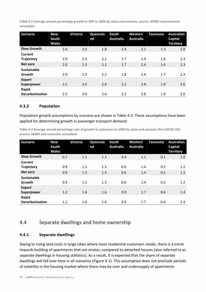
28 | CSIRO Australia’s National Science Agency
Table 4-2 Average annual percentage growth in GSP to 2050 by state and scenario, source: AEMO and economic
consultant
Scenario New South Wales
Victoria Queensland
South Australia
Western Australia
Tasmania Australian Capital Territory
Slow Growth 1.6 2.0 1.8 1.4 2.1 1.3 2.0
Current Trajectory 2.0 2.3 2.1 1.7 2.4 1.6 2.3
Net zero 2.0 2.3 2.1 1.7 2.4 1.6 2.3
Sustainable Growth 2.0 2.3 2.2 1.8 2.6 1.7 2.3
Export Superpower 2.5 3.0 2.6 2.2 2.8 1.9 2.6
Rapid Decarbonisation 2.5 3.0 2.6 2.2 2.8 1.9 2.6
4.3.2 Population
Population growth assumptions by scenario are shown in Table 4-3. These assumptions have been
applied for determining growth in passenger transport demand.
Table 4-3 Average annual percentage rate of growth in customers to 2050 by state and scenario (Pre-COVID-19),
source: AEMO and economic consultant
Scenario New South Wales
Victoria Queensland
South Australia
Western Australia
Tasmania Australian Capital Territory
Slow Growth 0.7 1.1 1.1 0.4 1.1 0.1 1.0
Current Trajectory 0.9 1.3 1.3 0.6 1.4 0.2 1.2
Net zero 0.9 1.3 1.3 0.6 1.4 0.2 1.2
Sustainable Growth 0.9 1.3 1.3 0.6 1.4 0.2 1.2
Export Superpower 1.2 1.6 1.6 0.9 1.7 0.4 1.4
Rapid Decarbonisation 1.2 1.6 1.6 0.9 1.7 0.4 1.4
4.4 Separate dwellings and home ownership
4.4.1 Separate dwellings
Owing to rising land costs in large cities where most residential customers reside, there is a trend
towards building of apartments that are stratas, compared to detached houses (also referred to as
separate dwellings in housing statistics). As a result, it is expected that the share of separate
dwellings will fall over time in all scenarios (Figure 4-1). This assumption does not preclude periods
of volatility in the housing market where there may be over and undersupply of apartments
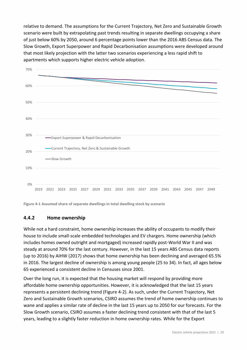
Electric vehicle projections 2021 | 29
relative to demand. The assumptions for the Current Trajectory, Net Zero and Sustainable Growth
scenario were built by extrapolating past trends resulting in separate dwellings occupying a share
of just below 60% by 2050, around 6 percentage points lower than the 2016 ABS Census data. The
Slow Growth, Export Superpower and Rapid Decarbonisation assumptions were developed around
that most likely projection with the latter two scenarios experiencing a less rapid shift to
apartments which supports higher electric vehicle adoption.
Figure 4-1 Assumed share of separate dwellings in total dwelling stock by scenario
4.4.2 Home ownership
While not a hard constraint, home ownership increases the ability of occupants to modify their
house to include small-scale embedded technologies and EV chargers. Home ownership (which
includes homes owned outright and mortgaged) increased rapidly post-World War II and was
steady at around 70% for the last century. However, in the last 15 years ABS Census data reports
(up to 2016) by AIHW (2017) shows that home ownership has been declining and averaged 65.5%
in 2016. The largest decline of ownership is among young people (25 to 34). In fact, all ages below
65 experienced a consistent decline in Censuses since 2001.
Over the long run, it is expected that the housing market will respond by providing more
affordable home ownership opportunities. However, it is acknowledged that the last 15 years
represents a persistent declining trend (Figure 4-2). As such, under the Current Trajectory, Net
Zero and Sustainable Growth scenarios, CSIRO assumes the trend of home ownership continues to
wane and applies a similar rate of decline in the last 15 years up to 2050 for our forecasts. For the
Slow Growth scenario, CSIRO assumes a faster declining trend consistent with that of the last 5
years, leading to a slightly faster reduction in home ownership rates. While for the Export
0%
10%
20%
30%
40%
50%
60%
70%
2019 2021 2023 2025 2027 2029 2031 2033 2035 2037 2039 2041 2043 2045 2047 2049
Export Superpower & Rapid Decarbonisation
Current Trajectory, Net Zero & Sustainable Growth
Slow Growth
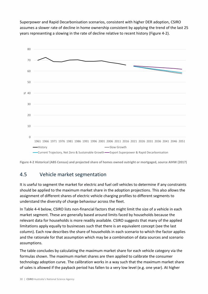
30 | CSIRO Australia’s National Science Agency
Superpower and Rapid Decarbonisation scenarios, consistent with higher DER adoption, CSIRO
assumes a slower rate of decline in home ownership consistent by applying the trend of the last 25
years representing a slowing in the rate of decline relative to recent history (Figure 4-2).
Figure 4-2 Historical (ABS Census) and projected share of homes owned outright or mortgaged, source AIHW (2017)
4.5 Vehicle market segmentation
It is useful to segment the market for electric and fuel cell vehicles to determine if any constraints
should be applied to the maximum market share in the adoption projections. This also allows the
assignment of different shares of electric vehicle charging profiles to different segments to
understand the diversity of charge behaviour across the fleet.
In Table 4-4 below, CSIRO lists non-financial factors that might limit the size of a vehicle in each
market segment. These are generally based around limits faced by households because the
relevant data for households is more readily available. CSIRO suggests that many of the applied
limitations apply equally to businesses such that there is an equivalent concept (see the last
column). Each row describes the share of households in each scenario to which the factor applies
and the rationale for that assumption which may be a combination of data sources and scenario
assumptions.
The table concludes by calculating the maximum market share for each vehicle category via the
formulas shown. The maximum market shares are then applied to calibrate the consumer
technology adoption curve. The calibration works in a way such that the maximum market share
of sales is allowed if the payback period has fallen to a very low level (e.g. one year). At higher
0
10
20
30
40
50
60
70
80
1961 1966 1971 1976 1981 1986 1991 1996 2001 2006 2011 2016 2021 2026 2031 2036 2041 2046 2051
%
History Slow Growth
Current Trajectory, Net Zero & Sustainable Growth Export Superpower & Rapid Decarbonisation

Electric vehicle projections 2021 | 31
payback periods, sales are less than the maximum market share. An exception is Net Zero,
Sustainable Growth, Export Superpower and Rapid Decarbonisation where, by design, the electric
and fuel cell vehicle adoption rate is set to achieve 100% of the fleet for cars, buses and rigid
(smaller) truck by 2055, 2050, 2045 and 2045 respectively.. This complete transformation of the
vehicle fleet to zero emission vehicles is consistent with the scenario narrative of net zero
greenhouse gas emissions in those scenarios.
In most cases, the market shares across vehicle types adds up to greater than 100%. As such they
should be interpreted as the maximum achievable share to be reached independent of
competition between vehicles. When applied in the model, the after-competition share is lower.
Note that autonomous ride share vehicles are assumed to be a subset of long-range electric
vehicles since this is the most natural vehicle type for this service (i.e. lowest fuel cost for high
kilometre per year activity). The market share limits are imposed on average. However, the
modelling allows individual locations (modelled at the ABS statistical area level 2) to vary
significantly from the average according to their demographic characteristics).

32 | CSIRO Australia’s National Science Agency
Table 4-4 Non-financial limitations on electric and fuel cell vehicle uptake and the calculated maximum market share
Current Trajectory
Slow Growth
Net zero
Sustainable Growth
Rapid Decarbonisation
Export Superpower
Rationale/formula Equivalent business constraint
Limiting factors (residential)
Separate dwelling share of households
A 58% 55% 58% 62% 62% 62% Based on housing industry forecasts Businesses located on standalone site
Share of homeowners B 59% 58% 59% 62% 62% 62% Based on historical trends Business not renting their site
Share of landlords who enable (passively or actively) EV charging onsite
C 70% 60% 70% 90% 100% 100% Data not available. Assumed range of 20-80%
Same
Off-street parking/private charging availability
D 41% 37% 44% 48% 49% 49% Assume 80% of separate dwellings have off-street parking. Formula=(0.8*A*B)+(0.8*A*(1-B)*C)
Same
Public or multi-occupant building charging availability
E 30% 25% 40% 60% 70% 70% Availability here means at your work/regular daytime parking area, apartment carpark or in your street outside your house. Assumptions are based on this type of charging being the least financially viable.
Same
Share of houses that have two or more vehicles
F 60% 58% 60% 65% 75% 75% Based on historical trends Share of businesses with two or more fleet vehicles
Share of houses where second vehicle is available for longer range trips
G 70% 67% 70% 75% 80% 80% Assumed range of 65-75%. There may be a range of reasons why second vehicle is not reliably available for longer trips
Operational availability of fleet vehicles
Share of people who would prefer ICE regardless of EV/FCEV costs or features
H 20% 25% 20% 0% 0% 0% Based on laggards generally being no larger than a third of customers. Sustainable growth assumes ICEs suffer a collapse in manufacturing due to systematic loss of supporting infrastructure
Business owner's attitudes and specific vehicle needs

Electric vehicle projections 2021 | 33
Current Trajectory
Slow Growth
Net zero
Sustainable Growth
Rapid Decarbonisation
Export Superpower
Rationale/formula Equivalent business constraint
Share of people who prefer private vehicle ownership for all household cars
I 90% 95% 90% 85% 85% 85% General preference for private vehicle ownership
Business preference for private ownership
Share of people willing for their second or more cars to be replaced with ride share
J 10% 5% 10% 15% 20% 20% Assumed that only a laggard proportion would object to this arrangement
Same
Fuel stations with access to hydrogen supply chain
K 10% 5% 10% 10% 10% 30% Data not available due to uncertainty. Assume range of 5-30%.
Same
Maximum market share
Short range electric vehicles
15% 12% 16% 25% 31% 31% Limitations are limited range and
charging. Due to range issue, assume SREVS only purchased by two or more car households and 10% of 1 car households. Formula=[(F*G*D)+(0.1*(1-F)*D)]*(1-H)
Large trucks 0%
Long range electric vehicles
57% 46% 67% 100% 100% 100% Key limitation is charging and
customer who would prefer ICE. Formula=(1-H)*(D+E)
Plug-in hybrid electric vehicles
57% 46% 67% 100% 100% 100% Same as long range
Fuel cell vehicles (light)
8% 4% 8% 10% 10% 30% Formula=(1-H)*K
Fuel cell large trucks 30% 50% 50% 90% Scenario setting
Autonomous ride-share vehicles
6% 3% 6% 10% 15% 15% Formula=J*F

34 | CSIRO Australia’s National Science Agency
Table 4-5 Shares of different electric vehicle charging behaviours by 2050 based on limiting factor analysis
Limiting factor Current Trajectory Slow Growth Net Zero
Sustainable Growth
Rapid Decarbonisation
Export Superpower Rationale/formula
Customers accessing tariffs that support prosumer behaviour and system integration L 20% 15% 25% 30% 35% 35% Scenario assumption
Residential vehicles
Home charging convenience profile 73% 78% 66% 59% 53% 53% Residual
Home charging night aligned (non-dynamic) 4% 3% 5% 6% 7% 7% Formula=0.2*L
Vehicle to home/grid (dynamic system-controlled charging) 12% 9% 18% 29% 35% 35% Formula=D*E
Public charging highway fast charge 5% 5% 5% 5% 5% 5% 90%+ of driving is within 30km of home
Public charging solar aligned (non-dynamic) 6% 5% 6% 1% 0% 0% Formula=0.8*(L-vehicle home/grid share)
Commercial vehicles
LCV - Convenience / night 74% 79% 69% 65% 60% 60% Non-highway kilometres. Formula=(1-L)*0.95
LCV - Daytime adjusted for solar alignment 19% 14% 23% 28% 32% 32% Non-highway kilometres. Formula=L*0.95
LCV highway fast charge 8% 8% 8% 8% 8% 8% Assume similar pattern to residential driving
Trucks & buses convenience / night 76% 81% 71% 67% 62% 62% Non-highway kilometres. Formula=(1-L)*0.95
Trucks & buses solar aligned 19% 14% 24% 29% 33% 33% Non-highway kilometres. Formula=L*0.95
Trucks & buses highway fast charge 5% 5% 5% 5% 5% 5% Assume similar pattern to residential driving

Electric vehicle projections 2021 | 35
4.6 Vehicle to home or grid
Once electric vehicles are established14, they will represent a large battery storage resource. For
example, if long-range electric vehicles are popular, each vehicle will represent around 100kWh of
battery storage – some nine times larger than the average 11kWh stationary batteries that are
marketed for shifting rooftop solar for households. It is therefore natural to consider whether this
battery storage resource could be used either after its life on board a vehicle or during that life.
The average vehicle in Australia travels 11,000km per year. For a SREV of 200km range the battery
size is around 40kWh, the average daily charge cycle will be 6.7kWh which is a depth of
charge/discharge of around 17%. If a driver were to travel 3 times that distance each year the shelf
life of the battery will run out before the cycle life. However, such a driver more than likely has a
long-range electric vehicle (due to their higher average kilometres per day) where the daily depth
of charge/discharge might be even lower.
Given the expected under-working of electric vehicle batteries it therefore makes sense to
consider how to get more use out of the battery while it is on the vehicle. Household yearly
average electricity demand is 6000kWh or 16.4kWh/day. As such, any full charged electric vehicle,
short or long range, can cover the required power needs with room to spare for the daily
commute. However, the most likely candidate for vehicle to home would be a long-range vehicle
with around 100-120kWh battery storage. An LREV could deliver energy to a home and would on
average only lose 100km or 20% or less of its 500+km range for the next day’s drive.
Vehicle to home would best suit a household that has access to charging via both home off-street
parking at their normal place of daytime parking (i.e. at work or in a carpark). Apart from getting
better utilisation out of an existing resource (the battery storage capacity in the vehicle), the other
financial incentive to this arrangement is the potential that the vehicle can charge up at lower
cost. This follows the general expectation that in the long term, as solar generation capacity
increases, the lowest priced period for electricity from the grid will be around midday. The
economics would also work well for the charging infrastructure provider. Instead of simply
providing electricity for each cars’ daily driving needs (around $2/day) they can instead provide
their car plus home needs ($6/day).
The process is achievable from a technical point of view with a more specialised connection to the
home. At least one current manufacturer has taken this concept forward overseas (the Nissan
Leaf).
The major difference with vehicle to grid is that it may push the boundaries further in terms of
utilisation of the vehicle battery to meet system needs. Presumably the business model in this
case would need to reach agreement with the vehicle owner on how much of the battery capacity
can be accessed so that the owner’s transport needs are not compromised. Potential faster and
deeper discharges could shorten the vehicle battery life. Nevertheless, the scale of electric vehicle
battery capacity in the higher EV uptake scenarios (even accounting for low availability and only
14 AEMO’s scenario design assumes this occurs post 2030

36 | CSIRO Australia’s National Science Agency
access half the battery) could be sufficient to avoid the need for major large-scale battery
deployment. As such, some compensation should theoretically be available to vehicle owners.
Our assumption is that commercial vehicles will not participate in either vehicle to grid or vehicle
to business (home). The rationale is that higher duty vehicles will have less excess capacity that
owners would be willing to make available to the grid. Commercial vehicles may still support the
system through non-dynamic pricing (tariffs).
4.7 Shares of electric vehicle charging behaviour
Besides setting the technology adoption saturation levels, the maximum market shares identified
in Table 4-4 are also applied, together with other assumptions, to determine what shares of
different electric vehicle charging profiles should be applied by 2050 (Table 4-5). The key
additional assumption is to assign the percentage of customers that are participating in tariffs or
other incentives for prosumer and electricity system supporting behaviour (which is a scenario
assumption).
For residential vehicles a small amount of highway charging is assumed consistent with the
observation from many trip studies that around 90% of driving is within local areas (see BITRE
2015). The amount of home charging is calculated from the amount of off-street parking
(calculated in Table 4-4). Charging at home is split between convenience and solar aligned
charging based on the tariff and other incentives assumptions. The formula allows for another
fraction of customers to participate in vehicle to grid or vehicle to home activities and charge
during the day at their daytime place of parking. This represents the subset of people who have
both off-street parking and access to public charging in that scenario.
Commercial charging profiles are aligned to the night time but could be incentivised to be aligned
with solar generation should that become the new off-peak period to support electricity system
efficiency (see Section 5.3 for charging profiles). Current tariffs faced by the commercial sector
also incentivise avoiding peak periods. It is assumed that signing up to new tariffs or incentives
could shift that part of charging which is not aligned with solar generation times into that time.
4.8 Transport demand
The future number of electric vehicles is partly determined by demand for transport and the
number of road vehicles required to meet that demand. To develop our road vehicle demand
projections, the process commences by projecting demand for passenger transport (passenger
kilometres or pkm) and freight transport (tonne kilometres or tkm) across all transport modes.
Passenger transport demand is a function of population, while freight demand is a function of
economic growth. Next, assumptions are made about the share of transport delivered by each
mode. In any normal year a simple extrapolation of past trends would be appropriate. For
example, the aviation transport mode has been steadily gaining market share in passenger
transport demand for decades. However, the COVID-19 pandemic has disrupted these trends and
is likely to have some degree of ongoing impacts. As a conservative approach the mode shares for
passenger transport are held constant at their current levels with only a slight leaning towards
previous trends. Freight transport mode shares were less impacted by COVID-19 and so historical
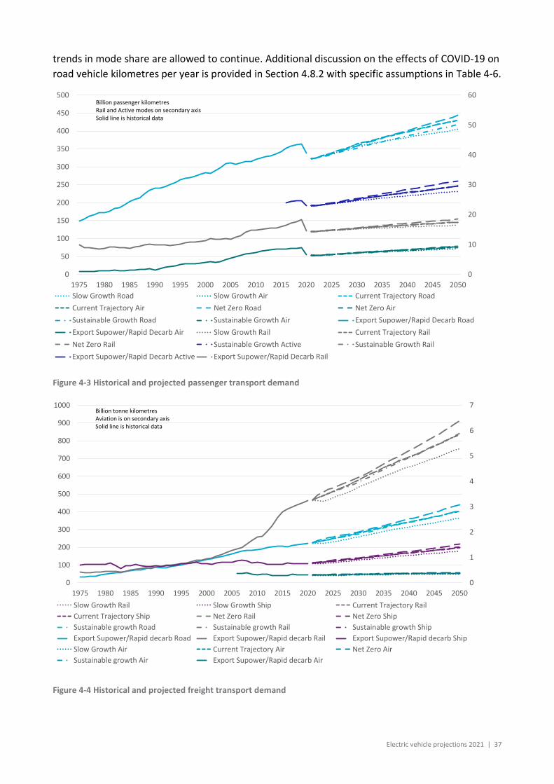
Electric vehicle projections 2021 | 37
trends in mode share are allowed to continue. Additional discussion on the effects of COVID-19 on
road vehicle kilometres per year is provided in Section 4.8.2 with specific assumptions in Table 4-6.
Figure 4-3 Historical and projected passenger transport demand
Figure 4-4 Historical and projected freight transport demand
0
10
20
30
40
50
60
0
50
100
150
200
250
300
350
400
450
500
1975 1980 1985 1990 1995 2000 2005 2010 2015 2020 2025 2030 2035 2040 2045 2050
Slow Growth Road Slow Growth Air Current Trajectory Road
Current Trajectory Air Net Zero Road Net Zero Air
Sustainable Growth Road Sustainable Growth Air Export Supower/Rapid Decarb Road
Export Supower/Rapid Decarb Air Slow Growth Rail Current Trajectory Rail
Net Zero Rail Sustainable Growth Active Sustainable Growth Rail
Export Supower/Rapid Decarb Active Export Supower/Rapid Decarb Rail
Billion passenger kilometresRail and Active modes on secondary axisSolid line is historical data
0
1
2
3
4
5
6
7
0
100
200
300
400
500
600
700
800
900
1000
1975 1980 1985 1990 1995 2000 2005 2010 2015 2020 2025 2030 2035 2040 2045 2050
Slow Growth Rail Slow Growth Ship Current Trajectory Rail
Current Trajectory Ship Net Zero Rail Net Zero Ship
Sustainable growth Road Sustainable growth Rail Sustainable growth Ship
Export Supower/Rapid decarb Road Export Supower/Rapid decarb Rail Export Supower/Rapid decarb Ship
Slow Growth Air Current Trajectory Air Net Zero Air
Sustainable growth Air Export Supower/Rapid decarb Air
Billion tonne kilometresAviation is on secondary axisSolid line is historical data

38 | CSIRO Australia’s National Science Agency
The results of these passenger and freight transport demand projections are shown in Figure 4-3
and Figure 4-4. The reduction in passenger transport demand during the COVID-19 pandemic is
strongly evident in the 2020 data. The data outlined in Figure 4-3 and Figure 4-4 are national, but
the projections are developed for each state and account for different levels of disruption from
COVID-19 by state.
To calculate road transport demand in vehicle kilometres CSIRO imposes a price elasticity
response by tracking future road transport costs (based on an initial estimate of the vehicle mix).
Views about autonomous vehicle adoption and the general level of vehicle utilisation are
discussed below.
4.8.1 Autonomous vehicles
As part of vehicle demand modelling, the uptake of automated vehicles in both the light and heavy
vehicle markets for private use and as ride share vehicles are projected. The main delay in
adopting these technologies is achieving complete safety and technological feasibility. Otherwise,
the benefits of time and wages saved from driving appear to be well above the vehicle cost on a
whole-of-life basis. The projections assume different market sizes over time across the scenarios
based around the general uncertainty to this new way of delivering road transport services.
Figure 4-5 shows the projected share of passenger and freight autonomous vehicles by scenario by
2050. Ride-share are disaggregated from privately owned autonomous vehicles. The total across
all vehicle types range from less than 1% to 20% across all scenarios by 2050. Rideshare vehicles
are of interest because they could reduce the total number of electric vehicles required on the
road and is likely to impact the total energy consumed under each vehicle charge profile.
Rideshare vehicles are only projected to reach a significant share in Sustainable Growth. While
these percentages are relatively small, each rideshare vehicle displaces other vehicles depending
on how successful they are in concentrating passengers into the rideshare vehicle. It is assumed
the displacement is initially small but increases such that each rideshare vehicle displaces 2 non-
rideshare vehicles by 2050 as the business model matures.

Electric vehicle projections 2021 | 39
Figure 4-5 Share of passenger and freight autonomous vehicles in the road vehicle fleet by scenario by 2050
4.8.2 Vehicle utilisation and numbers
To convert road passenger transport demand to vehicle numbers requires assumptions to be
made about average kilometres travelled per vehicle. According to ABS (2020), all passenger
vehicle types (motorcycles, passenger cars and buses) experienced a significant reduction in all
states (Figure 4-6) due to COVID-19. Buses suffered the strongest impact owing to the difficulty of
social distancing for passengers within such a vehicle. Light commercial vehicles and trucks
generally faired proportionally better with only modest reductions or increases in some states. In
short, Western Australia, Northern Territory and the Australian Capital Territory had the least
changes in vehicle utilisation.
The extent to which the COVID-19 pandemic will lead to sustained changes in vehicle utilisation is
uncertain. The experience has demonstrated to employers and employees that working from
home can be productively applied to some jobs. This has raised expectations that the option to
work from home may be available to employees well beyond the period in which such
arrangements are implemented purely for public health compliance reasons. The longer pandemic
conditions persist, such arrangements will be normalised. Therefore, it is not unreasonable to
expect that lower economic growth scenarios associated with lower population growth that
implies a slower recovery from the pandemic would reduce and maintain lower vehicle utilisation
into the future. Conversely, higher economic and population growth would suggest higher vehicle
utilisation. It is considered that the incidence of using telepresence for work and other activities
could increase as a greenhouse gas abatement strategy, particularly in scenarios with a net zero
emissions target. Based on this reasoning, assumptions for changes in vehicle utilisation were
developed and outlined in Table 4-6.
0%
5%
10%
15%
20%
25%
Slow Change Current Trajectory Net Zero Sustainable Growth Export Supower/RapidDecarb
Passenger Private AV Passenger AV ride-share Passenger AV bus Freight Private AV

40 | CSIRO Australia’s National Science Agency
Figure 4-6 Comparison of 2018-19 and 2019-20 vehicle utilisation by vehicle type
Table 4-6 Assumed changes in vehicle utilisation and rationale
Slow
Growth
Current
Trajectory
Net Zero Sustainable
Growth
Export
Superpower
Rapid
Decarbonisation
Extent to
which vehicle
utilisation
returns to pre-
COVID levels
75% of
difference
is
recovered
by 2030
75% of
difference
is
recovered
by 2030
75% of
difference
is
recovered
by 2030
25% of
difference is
recovered
by 2030
25% of
difference is
recovered
by 2030
25% of
difference is
recovered by
2030
COVID-19 has
accelerated
permanent
shift to greater
share working
from home
Somewhat Somewhat Somewhat Significantly Significantly Significantly
Climate policy
ambitions
encourage
greater use of
telepresence
Yes Yes Yes
0
10
20
30
40
50
60
70
80
90
100
Mo
torc
ycl
e
Pass
enge
r ca
r
Ligh
t co
mm
eric
al v
ehic
le
Rig
id t
ruck
Bus
Art
icul
ated
tru
ck
Mo
torc
ycle
Pass
enge
r ca
r
Ligh
t co
mm
eric
al v
ehic
le
Rig
id t
ruck
Bus
Art
icul
ated
tru
ck
Mo
torc
ycl
e
Pass
enge
r ca
r
Ligh
t co
mm
eric
al v
ehic
le
Rig
id t
ruck
Bus
Art
icul
ated
tru
ck
Mo
torc
ycle
Pass
enge
r ca
r
Ligh
t co
mm
eric
al v
ehic
le
Rig
id t
ruck
Bus
Art
icul
ated
tru
ck
Mo
torc
ycl
e
Pass
enge
r ca
r
Ligh
t co
mm
eric
al v
ehic
le
Rig
id t
ruck
Bus
Art
icul
ated
tru
ck
Mo
torc
ycle
Pass
enge
r ca
r
Ligh
t co
mm
eric
al v
ehic
le
Rig
id t
ruck
Bus
Art
icul
ated
tru
ck
Mo
torc
ycl
e
Pass
enge
r ca
r
Ligh
t co
mm
eric
al v
ehic
le
Rig
id t
ruck
Bus
Art
icul
ated
tru
ck
Mo
torc
ycle
Pass
enge
r ca
r
Ligh
t co
mm
eric
al v
ehic
le
Rig
id t
ruck
Bus
Art
icul
ated
tru
ck
NSW VIC QLD SA WA TAS NT ACT
Tho
usa
nd
km
/yea
r
2018-19 2019-20
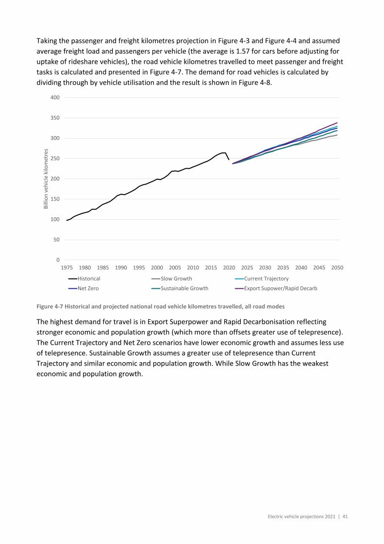
Electric vehicle projections 2021 | 41
Taking the passenger and freight kilometres projection in Figure 4-3 and Figure 4-4 and assumed
average freight load and passengers per vehicle (the average is 1.57 for cars before adjusting for
uptake of rideshare vehicles), the road vehicle kilometres travelled to meet passenger and freight
tasks is calculated and presented in Figure 4-7. The demand for road vehicles is calculated by
dividing through by vehicle utilisation and the result is shown in Figure 4-8.
Figure 4-7 Historical and projected national road vehicle kilometres travelled, all road modes
The highest demand for travel is in Export Superpower and Rapid Decarbonisation reflecting
stronger economic and population growth (which more than offsets greater use of telepresence).
The Current Trajectory and Net Zero scenarios have lower economic growth and assumes less use
of telepresence. Sustainable Growth assumes a greater use of telepresence than Current
Trajectory and similar economic and population growth. While Slow Growth has the weakest
economic and population growth.
0
50
100
150
200
250
300
350
400
1975 1980 1985 1990 1995 2000 2005 2010 2015 2020 2025 2030 2035 2040 2045 2050
Bill
ion
veh
icle
kilo
met
res
Historical Slow Growth Current Trajectory
Net Zero Sustainable Growth Export Supower/Rapid Decarb
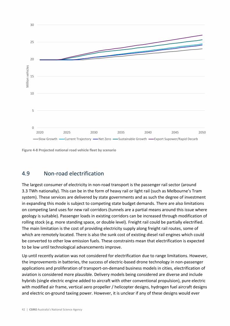
42 | CSIRO Australia’s National Science Agency
Figure 4-8 Projected national road vehicle fleet by scenario
4.9 Non-road electrification
The largest consumer of electricity in non-road transport is the passenger rail sector (around
3.3 TWh nationally). This can be in the form of heavy rail or light rail (such as Melbourne’s Tram
system). These services are delivered by state governments and as such the degree of investment
in expanding this mode is subject to competing state budget demands. There are also limitations
on competing land uses for new rail corridors (tunnels are a partial means around this issue where
geology is suitable). Passenger loads in existing corridors can be increased through modification of
rolling stock (e.g. more standing space, or double level). Freight rail could be partially electrified.
The main limitation is the cost of providing electricity supply along freight rail routes, some of
which are remotely located. There is also the sunk cost of existing diesel rail engines which could
be converted to other low emission fuels. These constraints mean that electrification is expected
to be low until technological advancements improve.
Up until recently aviation was not considered for electrification due to range limitations. However,
the improvements in batteries, the success of electric-based drone technology in non-passenger
applications and proliferation of transport-on-demand business models in cities, electrification of
aviation is considered more plausible. Delivery models being considered are diverse and include
hybrids (single electric engine added to aircraft with other conventional propulsion), pure electric
with modified air frame, vertical aero propeller / helicopter designs, hydrogen fuel aircraft designs
and electric on-ground taxiing power. However, it is unclear if any of these designs would ever
0
5
10
15
20
25
30
2020 2025 2030 2035 2040 2045 2050
Mill
ion
veh
icle
s
Slow Growth Current Trajectory Net Zero Sustainable Growth Export Supower/Rapid Decarb

Electric vehicle projections 2021 | 43
replace more than a few percent of long-haul high passenger load aviation. It is more likely that
electrification or hybrid engines will be adopted in shorter route low passenger load aviation.
The consideration of electrification of shipping is less common. This is because ships can use some
of the lowest cost liquid fuels available at present, their diesel engines are more easily adaptable
to alternatives such as very low sulphur fuel oils, LNG, biofuel, natural gas and hydrogen. The
weight of batteries and range limitation of electricity remains an unsolved issue. Consequently,
electrification of marine transport is not included in the projections.
The projections for passenger rail electricity consumption are based on the projected rail
passenger demand in Figure 4-3 multiplied by the extrapolated trend in rail energy requirements
per passenger kilometre. For rail freight and aviation electrification, CSIRO calculates their overall
energy demand and convert a share of demand over to electricity according to assumptions that
are presented in Table 4-7. These are a subjective assessment of technology readiness and
overcoming limits to adoption based on the scenario narratives.
Table 4-7 Rail freight and aviation electrification assumptions
Scenario Electrification commencement date
Rail freight Aviation
Maximum share by
2050
%
Slow Growth 2048 2047 3
Current Trajectory 2044 2042 5
Net Zero 2035 2030 7
Sustainable Growth 2035 2030 10
Export Superpower 2030 2027 20
Rapid decarbonisation 2030 2027 20

44 | CSIRO Australia’s National Science Agency
5 Projections results
In this section the projection results are presented here to 2055, as some of the assumptions
relate to years after the required projection period, such as the timing of internal combustion
vehicle deregistration in net zero emission scenarios. Some results in this section show all electric
vehicles engine types and these includes hydrogen electric vehicles while other results only
present battery electricity vehicles (BEVs). Selected CSIRO 2020 projections from AEMO’s 2020
scenario projections (Slow Change, Central and Step Change) are reproduced here for the
purposes of comparison (Graham et al., 2020).
5.1 Sales and fleet share
The projected sales and fleet shares for all electric vehicles compared to selected 2020 projections
are shown in Figure 5-1 and Figure 5-2 respectively. Previously, the 2020 Step change scenario
projections forced sales to reach 100% of electric vehicle by 2030 assuming there would be no
internal combustion vehicle available due to either global manufacturers switching out of internal
combustion vehicle supply or a government ban on sales of those vehicles (as has been announced
in some international countries). It is becoming more likely that global vehicle manufacturers will
no longer design and manufacturer internal combustion vehicles beyond a certain year. Public
announcements on cessation dates largely lie in years between 2030 through to 2040. As the
announcements are not universal with all car manufacturers, CSIRO now applies a range of 100%
electric vehicle sales across the scenarios: 2035 for Export Superpower and Rapid Decarbonisation,
2040 for Sustainable Growth, 2050 for Net zero, and beyond 2055 for the remaining scenarios.
In comparison, the 2020 Central and Slow change scenarios had no 100% sales date and instead
their sales saturated on the basis of assumed demographic and infrastructure constraints such as
access to charging (apartment buildings, no driveway/garage buildings and rented dwellings being
more difficult to arrange convenient home charging). The difference between the 2020 and the
2021 Current Trajectory and Slow Growth scenarios, is the 2021 projections assume these issues
are slowly overcome and does not cause a sales saturation effect. They are overcome because,
while the 100% sales date is much slower in comparison, CSIRO assumes it eventually does arrive
and it becomes an obligation of all landlords and apartment builders to provide charging points in
the future.
With historical scrappage rate in some states suggesting it may take up to 35 years to naturally
retire all internal combustion vehicles from the fleet, in order to represent scenario where road
transport emissions are eliminated, our approach does not solely rely on internal combustion
vehicles being unavailable for sale. A second strategy, to meet targets, should the government
choose, will be to set a date for disallowing registration renewal of internal combustion vehicles.
Our expectation is that this approach would probably only be used with a lot of lead time (e.g. ten
to fifteen years notice) so that current owners of internal combustion vehicles will be able to get
value out of their assets before they are no longer able to be registered. As such the deregistration
dates across the scenarios are set ten years after the 100% electric vehicle sales date. That is, 2045
for Export Superpower and Rapid Decarbonisation and 2050 for Sustainable Growth. For Net Zero,

Electric vehicle projections 2021 | 45
the date of 2055 is five years after the 100% electric sales data. This recognises that Net Zero
aligns most closely with Current Trajectory in the first decade after a policy shift requires net zero
emissions by 2050. It is assumed the road sector is not required to eliminate emissions by 2050
due to a later start in transforming the fleet but manages to achieve this goal five years later, by
2055, taking the pressure off the more difficult sectors for greenhouse gas emission abatement.
Figure 5-1 Projected sales share, all electric vehicles, compared to selected 2020 projections
Due to the different assumptions applied for vehicle cost reductions, both the sales and fleet share
projections display different timing of initial uptake. Short range electric vehicles are assumed to
cost the same as the equivalent size internal combustion vehicle by 2025 for Export Superpower,
Rapid Decarbonisation and Sustainable Growth, by 2030 in Current Trajectory and Net Zero, and
by 2035 in Slow Growth. The uncertainty around these dates is due to Australia’s different
approach to emission standards and mixed regional government approaches to subsidies and
rebates. This means Australia’s cost parity with EVs will differ to other international countries. In
other regions of the world, such as Europe, internal combustion vehicle costs are rising to meet
tighter emission standards and the range of vehicles available can be wider reflecting strong
government incentives.
0%
10%
20%
30%
40%
50%
60%
70%
80%
90%
100%
2015 2020 2025 2030 2035 2040 2045 2050 2055
Financial year ending
Slow growth Current trajectory Net zero Sustainable Growth
Rapid decarb/Export sup CSIRO Slow change CSIRO Central CSIRO Step change
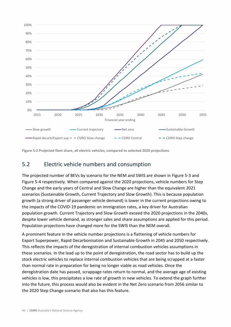
46 | CSIRO Australia’s National Science Agency
Figure 5-2 Projected fleet share, all electric vehicles, compared to selected 2020 projections
5.2 Electric vehicle numbers and consumption
The projected number of BEVs by scenario for the NEM and SWIS are shown in Figure 5-3 and
Figure 5-4 respectively. When compared against the 2020 projections, vehicle numbers for Step
Change and the early years of Central and Slow Change are higher than the equivalent 2021
scenarios (Sustainable Growth, Current Trajectory and Slow Growth). This is because population
growth (a strong driver of passenger vehicle demand) is lower in the current projections owing to
the impacts of the COVID-19 pandemic on immigration rates, a key driver for Australian
population growth. Current Trajectory and Slow Growth exceed the 2020 projections in the 2040s,
despite lower vehicle demand, as stronger sales and share assumptions are applied for this period.
Population projections have changed more for the SWIS than the NEM overall.
A prominent feature in the vehicle number projections is a flattening of vehicle numbers for
Export Superpower, Rapid Decarbonisation and Sustainable Growth in 2045 and 2050 respectively.
This reflects the impacts of the deregistration of internal combustion vehicles assumptions in
these scenarios. In the lead up to the point of deregistration, the road sector has to build up the
stock electric vehicles to replace internal combustion vehicles that are being scrapped at a faster
than normal rate in preparation for being no longer viable as road vehicles. Once the
deregistration date has passed, scrappage rates return to normal, and the average age of existing
vehicles is low, this precipitates a low rate of growth in new vehicles. To extend the graph further
into the future, this process would also be evident in the Net Zero scenario from 2056 similar to
the 2020 Step Change scenario that also has this feature.
0%
10%
20%
30%
40%
50%
60%
70%
80%
90%
100%
2015 2020 2025 2030 2035 2040 2045 2050 2055
Financial year ending
Slow growth Current trajectory Net zero Sustainable Growth
Rapid decarb/Export sup CSIRO Slow change CSIRO Central CSIRO Step change
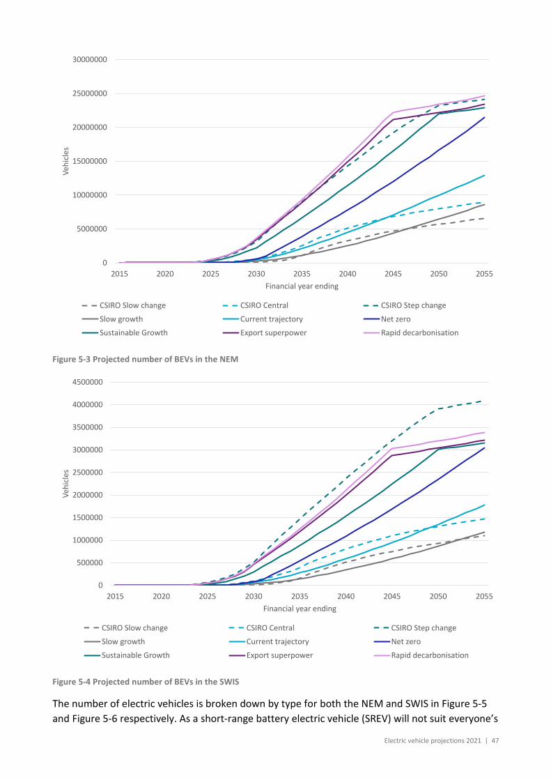
Electric vehicle projections 2021 | 47
Figure 5-3 Projected number of BEVs in the NEM
Figure 5-4 Projected number of BEVs in the SWIS
The number of electric vehicles is broken down by type for both the NEM and SWIS in Figure 5-5
and Figure 5-6 respectively. As a short-range battery electric vehicle (SREV) will not suit everyone’s
0
5000000
10000000
15000000
20000000
25000000
30000000
2015 2020 2025 2030 2035 2040 2045 2050 2055
Veh
icle
s
Financial year ending
CSIRO Slow change CSIRO Central CSIRO Step change
Slow growth Current trajectory Net zero
Sustainable Growth Export superpower Rapid decarbonisation
0
500000
1000000
1500000
2000000
2500000
3000000
3500000
4000000
4500000
2015 2020 2025 2030 2035 2040 2045 2050 2055
Veh
icle
s
Financial year ending
CSIRO Slow change CSIRO Central CSIRO Step change
Slow growth Current trajectory Net zero
Sustainable Growth Export superpower Rapid decarbonisation
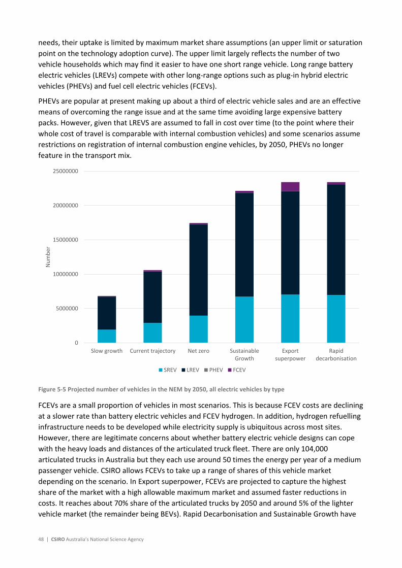
48 | CSIRO Australia’s National Science Agency
needs, their uptake is limited by maximum market share assumptions (an upper limit or saturation
point on the technology adoption curve). The upper limit largely reflects the number of two
vehicle households which may find it easier to have one short range vehicle. Long range battery
electric vehicles (LREVs) compete with other long-range options such as plug-in hybrid electric
vehicles (PHEVs) and fuel cell electric vehicles (FCEVs).
PHEVs are popular at present making up about a third of electric vehicle sales and are an effective
means of overcoming the range issue and at the same time avoiding large expensive battery
packs. However, given that LREVS are assumed to fall in cost over time (to the point where their
whole cost of travel is comparable with internal combustion vehicles) and some scenarios assume
restrictions on registration of internal combustion engine vehicles, by 2050, PHEVs no longer
feature in the transport mix.
Figure 5-5 Projected number of vehicles in the NEM by 2050, all electric vehicles by type
FCEVs are a small proportion of vehicles in most scenarios. This is because FCEV costs are declining
at a slower rate than battery electric vehicles and FCEV hydrogen. In addition, hydrogen refuelling
infrastructure needs to be developed while electricity supply is ubiquitous across most sites.
However, there are legitimate concerns about whether battery electric vehicle designs can cope
with the heavy loads and distances of the articulated truck fleet. There are only 104,000
articulated trucks in Australia but they each use around 50 times the energy per year of a medium
passenger vehicle. CSIRO allows FCEVs to take up a range of shares of this vehicle market
depending on the scenario. In Export superpower, FCEVs are projected to capture the highest
share of the market with a high allowable maximum market and assumed faster reductions in
costs. It reaches about 70% share of the articulated trucks by 2050 and around 5% of the lighter
vehicle market (the remainder being BEVs). Rapid Decarbonisation and Sustainable Growth have
0
5000000
10000000
15000000
20000000
25000000
Slow growth Current trajectory Net zero SustainableGrowth
Exportsuperpower
Rapiddecarbonisation
Nu
mb
er
SREV LREV PHEV FCEV

Electric vehicle projections 2021 | 49
around 30% of articulated trucks being hydrogen driven with smaller proportions in the remainder
of scenarios. There are no significant differences across the states except as driven by their share
of the trucking fleet15.
Figure 5-6 Projected number of vehicles in the SWIS by 2050, all electric vehicles by type
The trend in electricity consumption directly follows projected battery electric vehicle numbers
and outlined in Figure 5-7 and Figure 5-8. Lower Australian population projections, lower vehicle
numbers generally across the scenarios and lower kilometres travelled per day as a persisting
trend16 leads to lower electricity consumption compared to 2020 projections. The SWIS is more
impacted by population than the NEM, but it showed a smaller response to COVID-19 in terms of
changes in kilometres travelled per day. These opposing forces cancel out the changes in transport
activities, such that the SWIS changes in the range of electricity consumption projection compared
to 2020 is similar to the NEM.
15 That is, all states are assumed to reach the same share of fuel cell and electric vehicles, but they do not have the same share of trucks, cars and buses in their fleets
16 Due to a greater use of telepresence and work from home arrangements, due to changes to the workplace environment.
0
500000
1000000
1500000
2000000
2500000
3000000
3500000
Slow growth Current trajectory Net zero SustainableGrowth
Exportsuperpower
Rapiddecarbonisation
Nu
mb
er
SREV LREV PHEV FCEV
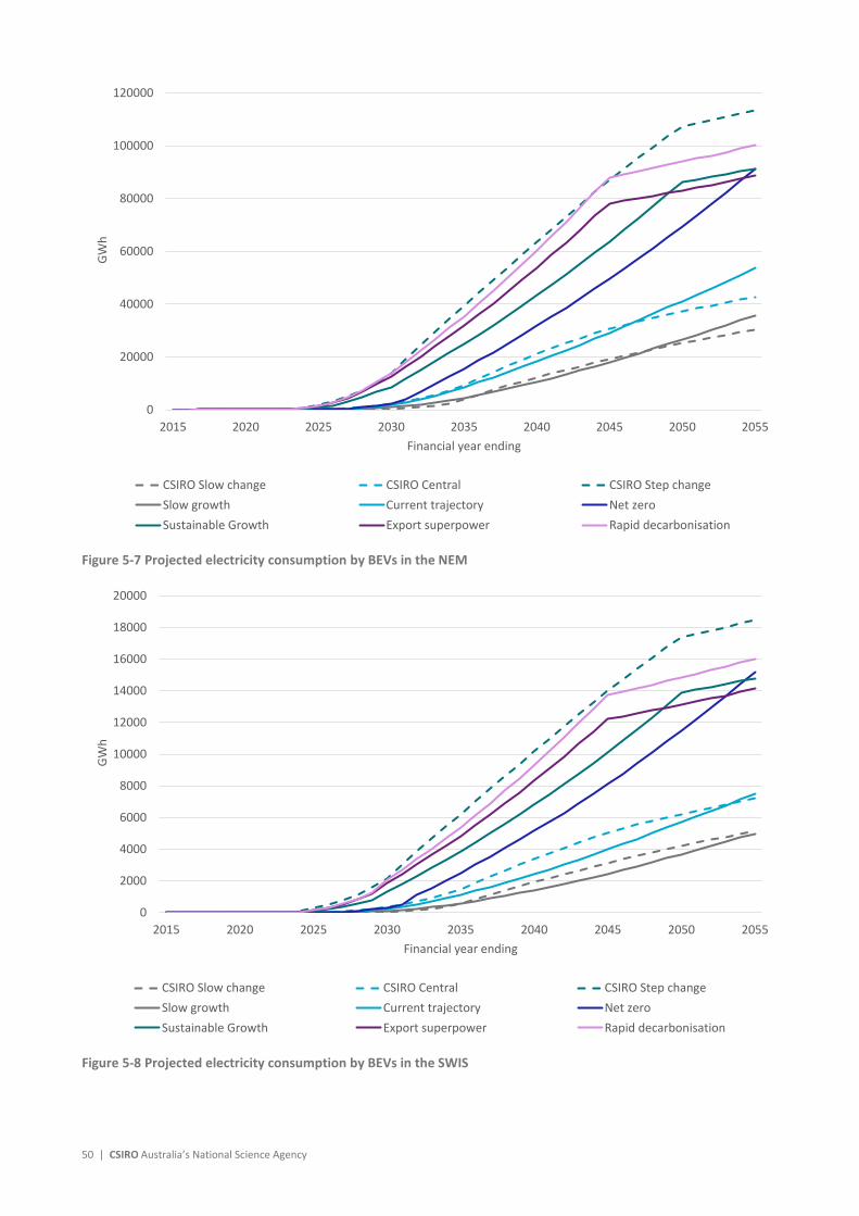
50 | CSIRO Australia’s National Science Agency
Figure 5-7 Projected electricity consumption by BEVs in the NEM
Figure 5-8 Projected electricity consumption by BEVs in the SWIS
0
20000
40000
60000
80000
100000
120000
2015 2020 2025 2030 2035 2040 2045 2050 2055
GW
h
Financial year ending
CSIRO Slow change CSIRO Central CSIRO Step change
Slow growth Current trajectory Net zero
Sustainable Growth Export superpower Rapid decarbonisation
0
2000
4000
6000
8000
10000
12000
14000
16000
18000
20000
2015 2020 2025 2030 2035 2040 2045 2050 2055
GW
h
Financial year ending
CSIRO Slow change CSIRO Central CSIRO Step change
Slow growth Current trajectory Net zero
Sustainable Growth Export superpower Rapid decarbonisation
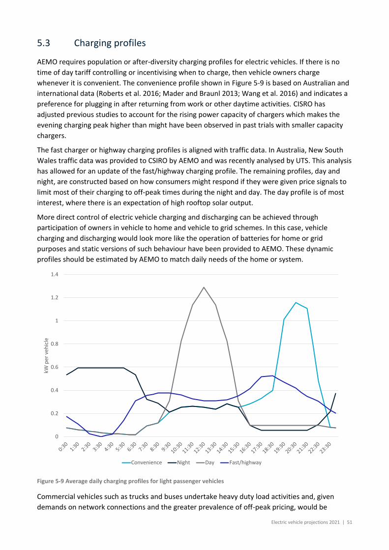
Electric vehicle projections 2021 | 51
5.3 Charging profiles
AEMO requires population or after-diversity charging profiles for electric vehicles. If there is no
time of day tariff controlling or incentivising when to charge, then vehicle owners charge
whenever it is convenient. The convenience profile shown in Figure 5-9 is based on Australian and
international data (Roberts et al. 2016; Mader and Braunl 2013; Wang et al. 2016) and indicates a
preference for plugging in after returning from work or other daytime activities. CISRO has
adjusted previous studies to account for the rising power capacity of chargers which makes the
evening charging peak higher than might have been observed in past trials with smaller capacity
chargers.
The fast charger or highway charging profiles is aligned with traffic data. In Australia, New South
Wales traffic data was provided to CSIRO by AEMO and was recently analysed by UTS. This analysis
has allowed for an update of the fast/highway charging profile. The remaining profiles, day and
night, are constructed based on how consumers might respond if they were given price signals to
limit most of their charging to off-peak times during the night and day. The day profile is of most
interest, where there is an expectation of high rooftop solar output.
More direct control of electric vehicle charging and discharging can be achieved through
participation of owners in vehicle to home and vehicle to grid schemes. In this case, vehicle
charging and discharging would look more like the operation of batteries for home or grid
purposes and static versions of such behaviour have been provided to AEMO. These dynamic
profiles should be estimated by AEMO to match daily needs of the home or system.
Figure 5-9 Average daily charging profiles for light passenger vehicles
Commercial vehicles such as trucks and buses undertake heavy duty load activities and, given
demands on network connections and the greater prevalence of off-peak pricing, would be
0
0.2
0.4
0.6
0.8
1
1.2
1.4
kW p
er v
ehic
le
Convenience Night Day Fast/highway

52 | CSIRO Australia’s National Science Agency
expected to be charging through the night mostly after the off-peak period (Figure 5-10). Hence
the “night” and convenience profile are the same. They are also assigned day and fast/highway
charging options.
Both the residential and commercial vehicle average daily charging profiles also consider further
improvements in EVs across scenarios. Within a year, these profiles are adjusted for differences in
weekend and weekday travel activity. Differences in monthly travel is also taken into account.
Over the forecast period, there are also additional annual adjustments for changes in the
efficiency of electric vehicles and in the average travelled distance per day.
Figure 5-10 Average daily charging profiles for rigid trucks
0
1
2
3
4
5
6
7
8
9
10
kW
Convenience Day Fast/Highway
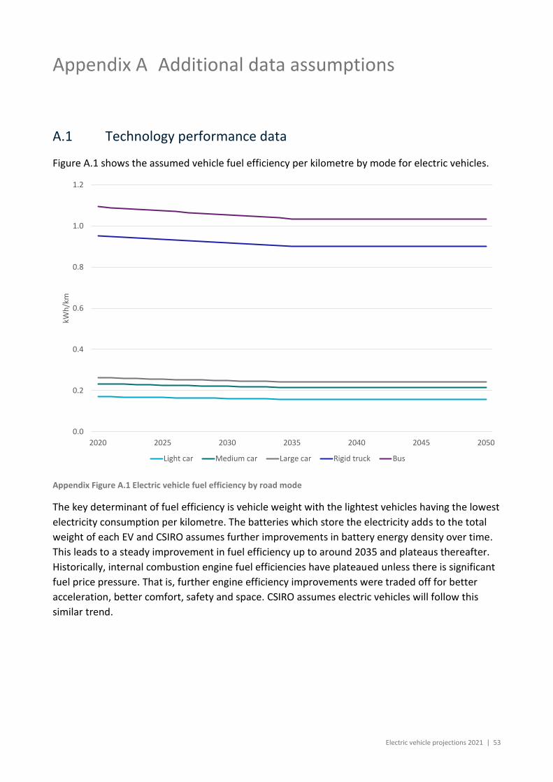
Electric vehicle projections 2021 | 53
Additional data assumptions
A.1 Technology performance data
Figure A.1 shows the assumed vehicle fuel efficiency per kilometre by mode for electric vehicles.
Appendix Figure A.1 Electric vehicle fuel efficiency by road mode
The key determinant of fuel efficiency is vehicle weight with the lightest vehicles having the lowest
electricity consumption per kilometre. The batteries which store the electricity adds to the total
weight of each EV and CSIRO assumes further improvements in battery energy density over time.
This leads to a steady improvement in fuel efficiency up to around 2035 and plateaus thereafter.
Historically, internal combustion engine fuel efficiencies have plateaued unless there is significant
fuel price pressure. That is, further engine efficiency improvements were traded off for better
acceleration, better comfort, safety and space. CSIRO assumes electric vehicles will follow this
similar trend.
0.0
0.2
0.4
0.6
0.8
1.0
1.2
2020 2025 2030 2035 2040 2045 2050
kWh
/km
Light car Medium car Large car Rigid truck Bus

54 | CSIRO Australia’s National Science Agency
Shortened forms
Abbreviation Meaning
ABS Australian Bureau of Statistics
ACCU Australian Carbon Credit Unit
AEMC Australian Energy Market Commission
AEMO Australian Energy Market Operator
APVI Australian Photovoltaic Institute
AV Autonomous Vehicle
BOP Balance of plant
CEFC Clean Energy Finance Corporation
CER Clean Energy Regulator
COVID-19 Coronavirus Disease of 2019
CSIRO Commonwealth Scientific and Industrial Research Organisation
DER Distributed energy resources
EE Energy Efficiency
ERF Emissions Reduction Fund
EV Electric Vehicle
FCAI Federal Chamber of Automotive Industries
FCAS Frequency Control Ancillary Services
FCEV Fuel Cell Electric Vehicle
GDP Gross Domestic Product
GSP Gross State Product
hrs Hours

Electric vehicle projections 2021 | 55
ICE Internal Combustion Engine
IPART Independent Pricing and Regulatory Tribunal
ISP Integrated System Plan
kW Kilowatt
kWh Kilowatt hour
LCV Light Commercial Vehicle
LGC Large-scale Generation Certificates
LRET Large-scale Renewable Energy Target
LREV Long-range electric vehicle
MW Megawatt
MWh Megawatt hour
NEM National Electricity Market
NSG Non-Scheduled Generation
PHEV Plug-in hybrid electric vehicle
pkm Passenger kilometres
PV Photovoltaic
QRET Queensland Renewable Energy Target
RET Renewable Energy Target
SA2 Statistical Area Level 2
SGSC Smart Grid Smart Cities
SREV Short-range electric vehicle
STC Small-scale Technology Certificates
SWIS South-West Interconnected System
tkm Tonne kilometres
56 | CSIRO Australia’s National Science Agency
TOU Time-of-use
TWh Terrawatt hour
UNFCCC United Nations Framework Convention on Climate Change
VPP Virtual Power Plant
VRE Variable Renewable Energy
VRET Victorian Renewable Energy Target
WEM Western Electricity Market

Electric vehicle projections 2021 | 57
References
Australian Bureau of Statistics (ABS) 2020, Survey of motor vehicle use, Australia, 12 months ended
30 June 2020, ABS.
Australian Energy Market Commission (AEMC) 2012, Directions paper: Power of choice - giving
consumers options in the way they use electricity, AEMC.
Australian Institute of Health and Welfare (AIHW) 2017, Australia’s welfare 2017, AIHW, Australia
Bass, F.M., 1969. A New Product Growth for Model Consumer Durables. Management Science, vol.
15, pp 215-227.
BCG 2015, Revolution in the driver’s seat: The road to autonomous vehicles
https://www.bcg.com/en-au/publications/2015/automotive-consumer-insight-revolution-
drivers-seat-road-autonomous-vehicles.aspx
Bureau of Infrastructure Transport and Regional Economics (BITRE) 2015, Australia’s commuting
distance: cities and regions, BITRE, Canberra.
Chen, L., Huang, X., Chen, Z. and Jin, L. 2016, Study of a new quick-charging strategy for electric
vehicles in highway charging stations, Energies, vol. 9, p744.
Climate Change Authority 2014, Light vehicle emission standards for Australia,
http://climatechangeauthority.gov.au/reviews/light-vehicle-emissions-standards-australia
CSIRO and Energy Networks Australia 2017, Electricity Network Transformation Roadmap: Final
report, ENA, Canberra.
FCAI (Federal Chamber of Automotive Industries) 2020, VFACTS report: New vehicles sales, FCAI.
Graham, P.W. and Havas, L. 2020, Projections for small-scale embedded technologies, CSIRO,
Australia.
Higgins, A., McNamara, C. and Foliente, G. 2014, Modelling future uptake of solar photo-voltaics
and water heaters under different government incentives, Technology forecasting and social
change, vol. 83, pp 142-155.
Higgins, A., Paevere, P., Gardner, J., Quezada G. 2012, Combining choice modelling and multi-
criteria analysis for technology diffusion: An application to the uptake of electric vehicles,
Technological Forecasting & Social Change, vol. 79, pp 1399–1412
KPMG 2018, Automated and zero emission vehicle infrastructure advice: Transport modelling,
Infrastructure Victoria.
Mader, T. and Bräunl, T. 2013, Western Australian electric vehicle trial 2010-2012,
http://therevproject.com/trialreport.pdf.
Roberts, D.A. 2016, My electric avenue: Learning and next steps, EA Technology
Rogers E., 1962. Diffusion of Innovations. Glencoe: Free Press

58 | CSIRO Australia’s National Science Agency
Stenner, K., Frederiks, E., Hobman, E. V., and Meikle, S. 2015, Australian consumers’ likely response
to cost-reflective electricity pricing. CSIRO, Australia
Victorian Government 2013, Creating a market: Victorian electric vehicle trial mid-term report,
State Government of Victoria, Melbourne.
Wang, H., Huang, X., Chen, L. and Zhuo, Y. 2016, Highway Electric Vehicle Charging Load Prediction
and its Impact on the Grid, 2nd International Forum on Electrical Engineering and
Automation (IFEEA 2015).


60 | CSIRO Australia’s National Science Agency
As Australia’s national science agency and innovation catalyst, CSIRO is solving the greatest challenges through innovative science and technology.
CSIRO. Unlocking a better future for everyone.
Contact us
1300 363 400 +61 3 9545 2176 [email protected] csiro.au
For further information
Energy Paul Graham +61 2 4960 6061 [email protected] csiro.au/energy