1

Electric Vehicle Fleet Management using Ant Colony

Optimisation

Javier Biera Muriel, Abbas Fotouhi *

Advanced Vehicle Engineering Centre, School of Aerospace, Transport and Manufacturing (SATM)

Cranfield University, Bedfordshire, MK43 0AL, UK

* Corresponding author, a.fotouhi@cranfield.ac.uk; abfotouhi@gmail.com

Highlights

Specific requirements of an EV fleet management system (FMS) are analysed and

a FMS case-study is simulated,

Ant Colony Optimisation (ACO) technique is used to develop a new ACO-based

EV FMS algorithm,

Comparing to other FMS algorithms such as the nearest-neighbour, ACO’s

performance is better, however, with additional computational time.

Abstract

This research is focused on implementation of the Ant Colony Optimisation (ACO)

technique to solve an advanced version of the Vehicle Routing Problem (VRP), called

fleet management system (FMS). An optimum solution of VRP can bring lots of benefits

for the fleet operators as well as contributing to the environment. Nowadays, particular

considerations and modifications are needed to be applied in the existing FMS algorithms

in response to the rapid growth of electric vehicles (EVs). For example, current FMS

algorithms don’t consider the limited range of EVs, their charging time or battery

degradation. In this study, a new ACO-based FMS algorithm is developed for a fleet of

EVs. A simulation platform is built in order to evaluate performance of the proposed FMS

algorithm under different simulation case-studies. The simulation results are validated

against a well-established method in the literature called Nearest-Neighbour technique.

At each case-study, the overall mileage of the fleet is considered as an index to measure

the performance of the FMS algorithm.

Keywords: Ant colony optimisation; vehicle routing problem; electric vehicle; fleet

management systems.

2

1. Introduction

The Travelling Salesman Problem (TSP) is defined as a salesman that is required to visit

“n” given cities just once, departing from a city or depot and returning to the same point

(Lin, 1965). The concern is which of the possible routes is the shortest so the salesman

can travel the least. For almost sixty years this problem has been approached from quite

a large variety of methods (Ma, Yang, Hou, Tan, & Liu, 2007; Saji & Riffi, 2015;

Ouaarab, Ahiod, & Yang, 2013). TSP has real applications in engineering problems as

well; a good example is the Vehicle Routing Problem (VRP) that can be considered as

form of TSP in which a vehicle is planned to visit a number of cities (Christofides, 1976).

Mathematically, the problem can be defined as a graph G = (V, A) where V = {1,…,n} is

a set of vertices that represent cities or customers with the depot located in vertex 1, and

A is a set of arcs. Every arc (i, j) i≠j is associated to an element in the distance symmetrical

matrix C=(cij) (Laporte, 1992). The aim of the TSP is to minimise the total distance (or

cost) covered by the salesman. Let xij (i≠j) be a binary variable equal to 1 if and only if

the arc (i, j) appears in the optimal solution; therefore, the main objective of the TSP is to

find the most optimal route to be followed (Laporte, 1992):

𝒎𝒊𝒏 ∑ 𝒄𝒊𝒋 ∗ 𝒙𝒊𝒋𝒏𝒊≠𝒋 (1)

The way to find the exact solution for the TSP is to calculate all the possible routes and

get the best one (depending on the cost function). This can only be implemented if the

number of cities or customers is very small. However, as the number of cities increases,

the possibilities grow exponentially and the direct search method wouldn’t work. So, an

advanced optimisation algorithm is needed to be implemented. Along the years, several

approaches have been studied in order to solve this problem. One solution is the Nearest

Neighbour algorithm that suggests travelling to the closest neighbour from the salesman’s

current position, which is also named as the “greedy algorithm”. Although the process is

fairly rapid, a visual analysis shows that the route is far to be optimal: the first distances

will tend to be very small, while the last ones are often very large (Boone, Sathyan, &

Cohen, 2015). A useful extension of the TSP is called Multiple Travelling Salesmen

Problem (MTSP). An application of MTSP is in VRP where a number of vehicles visit

all the given cities (target points). Nature has served as a window display for several

3

algorithms to solve the TSP in its different variations and mobile robots path planning

(Palmieri, Yang, Rango, & Marano, 2017; Chen, Kong, Fang, & Wu, 2011). Genetic

Algorithm, Metal Annealing, Neural Networks, Tabu Search and Ant Colony are good

examples for this.

A new application of the MTSP which is also considered in this study, is electric vehicle

(EV) fleet management system (FMS). There are few studies in the literature focusing on

this topic. In a study by Betz, Werner, & Lienkamp (2016), a mixed fleet of non-electric

and electric vehicles was assessed. Then, a new model was developed to investigate the

financial and ecological influences of replacing conventional vehicles with EVs to

generate a personalized optimal fleet composition according to the number of trips and

vehicle specifications. In a study by Hu, Morais, Sousa, & Lind (2016), a review of the

optimization and control methods of intelligent EV fleet charging is discussed and the

fleet operator services to other actors in a smart grid are presented. In a study by Chen,

Kockelman, & Hanna (2016), operation of an autonomous EV fleet has been studied by

doing simulations. The results have shown that the size of the fleet should be determined

based on the charging infrastructure and vehicle range. In another study by Chao &

Xiaohong (2013), differences between a fleet of electric buses and a fleet of diesel buses

are assessed. It is shown that such differences need significant changes in vehicle

scheduling methods when switching from diesel to electric.

Going through the comparative studies of the theoretical methods that can be considered

for VRP, the Ant Colony Optimisation (ACO) technique is one of the most promising

techniques in the literature (Tarasewich & McMullen, 2002). ACO algorithm copies the

behaviour of insects, specifically ants due to the clarity of their conduct and big research

behind. It is possible to apply ACO in MTSP by using multiple colonies since the multiple

colony approach is shown to perform better for larger problems (Bell & McMullen, 2004).

Algorithms like ACO that get the intelligence from individual elements can perform

better than the others that work based on a central thinking system (Johnson, 2001). This

advantage is quite relevant and applicable to VRP. FMS problem that is studied here, can

be considered as a particular type of VRP. Furthermore, ACO can be combined with other

algorithms which copy swarm intelligence improving mileage results (Goel and Maini,

2018).

4

This study is focused on design and simulation of a FMS algorithm for managing a fleet

of commercial EVs. The idea is to utilise an optimisation technique to minimise the

overall fleet mileage while visiting a number of target points which are randomly

distributed in a surrounded area. Vehicles depart and return to a depot which is located at

the centre of the area. Simultaneously, the depot is served as the only charging point

(overnight slow charging). This case-study has been introduced in a previous study and a

solution was obtained for it using Nearest-Neighbour technique (Fotouhi, et al., 2016). In

this study, firstly the Nearest-Neighbour FMS algorithm is improved and secondly, a new

FMS algorithm is developed based on ACO technique. Performances of both algorithms

are simulated and results are compared. Although, this is not the first time ACO is been

used to solve a VRP (Abousleiman & Rawashdeh, 2014) or the original TSP (Jaradat,

2018). Standing out among the literature, this study is novel in terms of the application of

ACO for FMS. In addition, particular requirements of an EV fleet are considered such as

EVs’ limited travel range and battery degradation minimisation via slow charging

overnight.

2. EV Fleet Management System

Considerations of an EV Routing Problem

The main differences, in terms of practicality, between VRP and Electric Vehicle Routing

Problem (EVRP) is the necessity of considering the recharging process of the EV battery

and its shorter range in comparison to the conventional vehicles (Murakami, 2017). There

are different EV charging technologies such as slow charging at depots, fast and super

charging between journeys or battery swapping. Each charging technology has its

advantages and disadvantages which are out of the framework of this study. The other

difference is the EV’s range that should be considered when vehicles are dispatched in

order to guarantee enough charge to return to depot. In this study, slow charging at depot

is considered and the proposed FMS algorithm is able to handle the EV range limitation.

Since charging between journeys is not considered here, the issues due to the charging

time are not investigated in terms of time management (assuming slow charging over

night at depot) however, this is an important subject which should be addressed in future

studies as mentioned in the literature as well (Erdoĝan & Miller-Hooks, 2012; Schiffer &

5

Walther, 2017). This is important because fleet operator companies tend to use their fleet

at the maximum capacity per day in order to amortize and renew it using the latest

technologies. In addition to the charging time, battery degradation and disposal should be

also considered. Usually a proper trade-off is needed to make a balance between the

charging time and battery degradation. Battery State of Health (SoH) is a quite important

factor for today’s devices (Barco, Guerra, Muñoz, & Quijano, 2017).

FMS Case-Study

The case-study that is considered here includes an optimisation problem in which the

overall mileage of a fleet of commercial vehicles is minimised while visiting certain

number of target points in a surrounded area. Vehicles depart from and return to a depot

which is located at the centre of the area. The depot is served as the only charging point

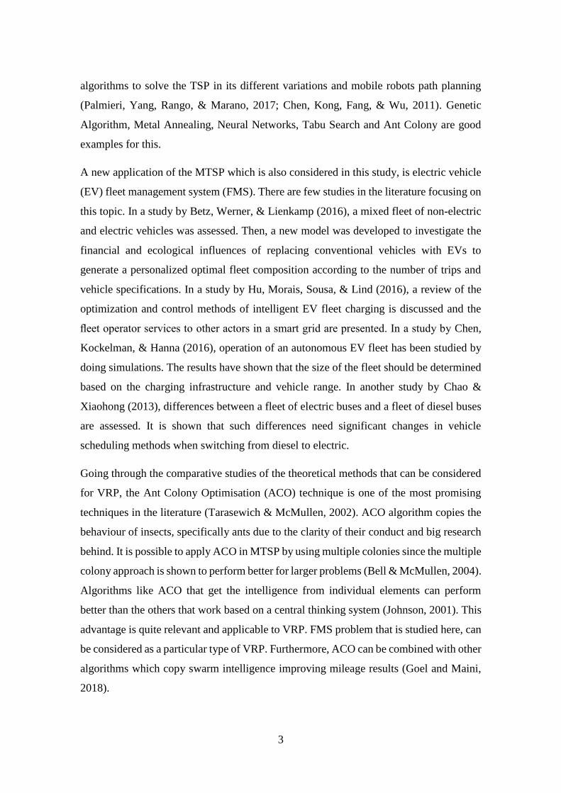
(overnight slow charging). The target points are randomly distributed in a 50 × 50 𝑘𝑚2

area. Different densities are also investigated by changing the number of target points in

the same area (50, 200, and 500 points for low, medium and high density cases) as shown

in Fig. 1.

Regarding the slow charging scenario in this case-study, the scheduling plan is prepared

for the next day by assuming that target points are known from a day before (an example

of this application is the delivery tasks which are performed by commercial fleets). So,

each EV starts its journey at fully charged state every day and operates until no more

charge is available (by considering the required charge to return to the depot). In terms of

the optimisation problem’s complexity, this is a simpler case comparing to a dynamic

demand scenario like a fleet of taxi where the next target point is unknown. The reason

for choosing the simpler scenario in this study, is the time needed for performing the

optimisation using ACO (quick real-time optimisation is left for future studies).

Therefore, the role of the FMS algorithm is to allocate the target points to a number of

EVs (depending on the number of target points and their distances) in a way to minimise

the overall mileage of the fleet. The main constraint here is the range of EV (i.e. identical

for all EVs in the fleet). The FMS algorithm would try to use each EV as much as possible

however, it should guarantee enough charge for each EV to return to the charging depot

6

after completing its task. For the sake of simplicity, no vehicle dynamics, nor topography

considerations, nor energy recovery by kinematics or heat is implemented in this study.

Fig. 1: Random distribution of target points: (a) low density, (b) medium density, and (c) high

density

The minimum range of EVs to operate in a 50 × 50 𝑘𝑚2 area is determined based on a

previous study by Fotouhi, et al., (2016) in the literature that suggests a range of 125 km

for a similar size area. It should be noted that the main conclusions of this study are not

expected to be affected by changing the range of EV. Because the only effect on results

when for example we have double range (250 km), is to dispatch less EVs however, the

7

effect is similar to the change of target points’ density which is considered in this study.

The effectiveness of ACO technique for FMS application is investigated based on the

above mentioned case-study however, it is extendable to other case-studies as well.

3. A New Algorithm for EV FMS using ACO

In this study, a new EV FMS algorithm is developed using ACO technique. Performance

of the proposed algorithm is simulated and analysed for the case-study explained in

Section 2.2. As a benchmark to evaluate the simulation results, the Nearest-Neighbour

FMS algorithm is also implemented and the results are compared. The two techniques are

fundamentally different; while the Nearest Neighbour-based FMS algorithm always tends

to travel to the closest point from the current position, the ACO-based FMS algorithm

considers a wider range of different options to travel.

A basic version of the Nearest Neighbour-based FMS algorithm has been developed in

the literature by Fotouhi, et al., (2016). However, in this study, improved versions of the

Nearest Neighbour technique are proposed and used that are called 2 Point Optimisation

(2-Opt) and 3 Point Optimisations (3-Opt) Nearest Neighbour algorithm. In both

algorithms, the original signal that is obtained from Nearest Neighbour is rechecked for

possible improvements by selecting consecutive points and evaluating all possible

scenarios to pass them to find the shortest one. In 2-Opt, each two consecutive points are

rechecked whereas in 3-Opt, same procedure is performed for each three consecutive

points. These techniques are helpful when a route line crosses itself. This is a very

common situation in Nearest Neighbour, especially in high city density scenarios.

Computation time increases, although the reduction in overall mileage over additional

time is worth the effort (Lin, 1965).

The Nearest Neighbour-based FMS algorithm is used in this study just as a benchmark to

evaluate ACO-based FMS algorithm.

Introduction to ACO

While an ant is walking it leaves pheromones along the path, the artificial pheromones in

the ACO algorithm represent the desirability of a path. The more ants decide to take that

path the more pheromones will be deposited and then the route is identified as a desired

8

route (Narasimha & Kumar, 2011). The more ants are over the graph, the more

information will be available and consequently a better result might be achievable.

Nevertheless, the technique requires additional computational effort. There are three clues

to understand the formation of optimum paths with ACO: “(i) the preference for paths

with a high pheromone level, (ii) the higher rate of growth of the amount of pheromone

on shorter paths, and (iii) the trail mediated communication among ants” (Dorigo &

Gambardella, 1997). In addition, ‘artificial’ ants have the memory of the visited points so

they can perform the whole TSP (Bell & McMullen, 2004). In such a scenario, ants are

guided along the possible routes between cities. In these kind of self-learning algorithms

the solution is not unique and might change at every attempt.

The ACO equations are designed to give a percentage of randomness in finding the

solutions that can help to avoid ‘local minima’ solutions. In general, it is very difficult to

find the ‘global minima’ for TSP especially when the number of points increases. So, here

we are talking about semi-optimum solutions and there is no mathematical prove that the

result of ACO is the best. As mentioned before, the nearest-neighbour algorithm is used

as a benchmark in all the simulation cases in order to have a better judge about the ACO

performance.

Parameter initialisation is something important that the ACO’s performance relies on it.

Indeed, using the most suitable parameters is a matter of fact to get the best results. The

ACO initialisation process contains determination of general parameters such as the

number of iterations and the number of ants (which affect the simulation time and the

algorithm convergence) and also more specific parameters (listed in Table 1) which affect

the algorithm’s performance in terms of ant behaviour. Table 1 gives a brief explanation

about four main parameters in ACO. In this study, the ACO parameters are tuned by

repeating the simulations using different set of parameters and considering the average

performance.

9

Table 1: ACO Parameter Explanation

Parameter Description

Evaporation ratio, ρ (rho) This parameter defines the percentage of pheromones that

remain after every iteration, ρ changes between 0 and 1

Pheromone exponential

weight, α (alpha)

This parameter weights the amount of initial and new

pheromones when pheromone concentration is updated, α

changes between 0 and 1

Heuristic exponential

weight, β (beta)

This parameter weights the distance and pheromone trail, β

changes between 0 and ∞

Next customer selection

parameter, Q0

This is compared with q (random) to choose equation for next

customer selection, Q0 changes between 0 and 1

FMS Algorithm using ACO

In this study, a novel FMS algorithm is developed for a fleet of EVs to operate based on

the case-study presented in Section 2.2. ACO technique is used as the main part of the

proposed FMS algorithm. Literature has covered ACO to solve the EV routing problem,

even going further in complexity than this paper’s approach, such as Zhang et al. (2018).

However, this research brings to front page the fleet behaviour using ACO, which is not

considered in literature. The algorithm is developed and simulated using MATLAB

software. As a starting point of the code generation process, a basic ACO code is used

from the literature (Heris, 2015). Essential changes have been applied to the original ACO

algorithm in order to make it applicable for EV FMS. As a result, a new algorithm has

been developed as shown in Fig. 2 in form of a flow chart. One of the main changes

applied in the baseline ACO code to propose an ACO-based FMS algorithm is the

inclusion of several EVs. While the baseline algorithm performs the whole problem with

one agent (i.e. a vehicle in this case), the proposed FMS algorithm is able to dispatch

several EVs due to their limited range. Furthermore, the proposed algorithm has different

parts including initialisation, iterations, ants’ state updating (inside iterations) and ants’

pheromone updating. There are five main functions in the algorithm: 1) determination of

the first point to start, 2) investigation of possible points to travel next, 3) selection of the

next point to travel, 4) pheromone updating, and 5) pheromone evaporation. The number

of iterations and the number of ants are initialised at the beginning.

10

Determination of the first point to travel can be performed by a random function, so any

city can be chosen. This piece of randomness in the FMS algorithm can lead to some gain

in the performance since it contributes to algorithm’s exploration. However, a previous

study in the literature by Fotouhi, et al. (2016) demonstrates that the initial point in such

a FMS case-study is quite important. Although, the results are shown for Nearest

Neighbour-based FMS algorithm, this can be extended to ACO algorithm as well. To

investigate this further, both the random (normal) initialisation and ‘best point’

initialisation approaches are simulated in Section 4. The ‘best point’ initialisation

approach comes from the literature (Fotouhi, et al., 2016) where all the existing points

are tested as the initial point at the beginning and the one that gives the best result is

selected. Previous research shows an impressive improvement with the implementation

of the best initial condition for Nearest Neighbour technique. In this study, firstly the best

initial condition is determined using the Nearest Neighbour technique and then ACO

starts from that point instead of a random point. The process of ‘best initialisation’ can be

performed only for the first EV or it can be repeated every time when a new EV is

dispatched (i.e. for all EVs at the beginning of their journeys). The results of all

initialisation techniques are investigated in Section 4.

After travelling to the first point, all other points are considered as a possible candidate

to be the second point. However, some of them might not be feasible because of the EV

range limitation. In addition to the unfeasible points in term of EV range, the visited points

should be also eliminated from the list of possible next points. This will be the input for

the next customer function that selects the next point by comparison of two variables Q0

(parameter, 0≤Q0≤1) and q (random variable with uniform probability, [0,1]) as follows

(Dorigo & Gambardella, 1997; Bell & McMullen, 2004):

𝑖𝑓 𝑄0 ≤ 𝑞 𝑗 = 𝑎𝑟𝑔𝑚𝑎𝑥𝑜𝑡ℎ𝑒𝑟𝑤𝑖𝑠𝑒 𝑆

{(𝜏𝑖𝑢)(η𝑖𝑢)𝛽} 𝑢 ∉ 𝑀𝑘 (2)

where 𝑖 is the current position and 𝑢 is the next one, τ is the pheromone concentration, η

is a heuristic function taken from the inverse of the distance between cities 𝑖 and 𝑢, β is a

parameter that weighs the distance and pheromone trail (β>0), 𝑀𝑘 is a vector that contains

all visited cities. The parameter 𝑠 is a random variable based on the probability

11

distribution 𝑃, it will favour short routes with high level of pheromones (Bell &

McMullen, 2004):

𝑃𝑖𝑠 = (𝜏𝑖𝑠)(𝜇𝑖𝑠)𝛽

∑ (𝜏𝑖𝑢)(𝜇𝑖𝑢)𝛽𝑢∈𝑀𝑘

𝑠 ∉ 𝑀𝑘

𝑜𝑡ℎ𝑒𝑟𝑤𝑖𝑠𝑒 0 (3)

Pheromone updating for TSP has been approached from the point of view that every ant

affects the pheromone concentration as it happens in real life. However, previous research

in EVRP models show that better behaviour is observed when pheromones are updated if

and only if a better solution is reached, hence, not all ants will contribute to pheromone

updating (Abousleiman & Rawashdeh, 2014). The pheromone updating equation will

select a percentage of the initial and new pheromones (Bell & McMullen, 2004):

𝜏𝑖𝑗 = (1 − 𝛼)𝜏𝑖𝑗 + (𝛼)𝜏0 (4)

where α is a parameter that weighs the amount of initial and new pheromone that will

remain (𝛼(0, 1)), 𝑖 and 𝑗 are the current and next position, τ0 is the initial pheromone

concentration ruled by the following formula (Heris, 2015):

𝜏𝑜 = 10∗ 𝑄0

𝑛𝑢𝑚𝑏𝑒𝑟 𝑜𝑓 𝑐𝑖𝑡𝑖𝑒𝑠∗𝑚𝑒𝑎𝑛(𝑑𝑖𝑠𝑡𝑎𝑛𝑐𝑒 𝑚𝑎𝑡𝑟𝑖𝑥) (5)

Pheromone evaporation takes place before the start of a new iteration (Heris, 2015):

𝜏𝑖𝑗 = (1 − 𝜌)𝜏𝑖𝑗 (6)

Where ρ is the evaporation ratio.

Referring to Fig. 2, inside every iteration loop, there is another loop regarding the number

of ants. At the end of each stage, a cost function is calculated (i.e. the overall mileage of

the fleet) and the new solution is saved if it outperforms the previous best solution. The

same check is done when updating the pheromone concentration via Equation 4. Before

going to the next iteration, the best solution is updated if necessary so the algorithm can

keep on improving. Additionally, parameters will ensure proper development of the

solutions as explained before. The solution might not improve after a certain number of

iterations. This is due to a stabilisation in pheromone concentration over the best solution

or sometimes an excessive pheromone evaporation.

12

Fig. 2: ACO-based FMS algorithm’s flow chart

13

4. FMS Simulation and Results Analysis

In this section, the proposed ACO-based FMS algorithm is simulated for the case-study

explained in Section 2.2. For each simulation case, the overall mileage of the fleet is

considered as the ‘cost function’ to evaluate performance of the FMS algorithm. Indeed,

a better performance is defined in a way to achieve less total mileage while reaching all

the target points (i.e. the constraint of the optimisation problem).

In order to have a comprehensive study of the ACO-based FMS algorithm, adjustable

parameters of the ACO algorithm are changed and performance of the fleet is investigated

in each case separately. In addition, the effect of initial condition on FMS performance is

investigated.

FMS simulation using different values of ACO parameters

In this section, the effects of ACO parameters on the FMS performance are investigated

including the number of ants, the number of iterations, pheromone evaporation rate,

pheromone concentration, weighting of pheromone trail with distance, and next city

selection process. All the simulation cases are performed for the medium density (as

defined earlier in this article) to keep consistency.

Number of ants

To investigate the impact of the number of ants on FMS performance, the FMS case-

study is simulated using different numbers of ants. Table 2 contains average and the best

results of FMS algorithm in term of the total fleet mileage using different number of ants

varying from 20 to 100. The results demonstrate that increasing the number of ants

doesn’t necessarily improve the FMS performance. This result can be explained in a way

that having more ants implies more pheromone information, hence less accuracy from a

certain value. On the other hand, having less ants would lead to lack of pheromone

concentration. So, an optimum number of ants can be obtained for each application that

is 50 ants in this case based on Table 2.

14

Table 2: the effect of number of ants on overall fleet mileage

number of ants average result

(km)

the best result

(km)

20 723.29 690.40

50 707.25 682.22

75 714.02 701.37

100 712.86 707.14

Number of iterations

According to the theory of ACO, by running the algorithm longer, the better results might

be achieved but with additional computational time. So, a proper trade-off is needed to

determine the optimum number of iterations based on the required level of accuracy in

each application. Table 3 contains average and the best results of FMS algorithm in terms

of the total fleet mileage using different number of iterations. As stated in the table, the

simulation is performed by considering 200, 500, and 1000 iterations. It should be noted

that each simulation case is repeated a number of times to avoid inaccuracy due to the

randomness that exists in ACO algorithm. Both average and best result are presented for

each case in Table 3. The results demonstrate that more iterations improve the results

however, the rate of improvement decreases after a certain number of iterations. At that

point, the computational time increases without enough benefit in terms of FMS

performance that means a proper trade-off is needed between them. According to the

results presented in Table 3, the number of iterations is set at 500.

Table 3: The effect of number of iterations on overall fleet mileage

number of

iterations

average result

(km)

the best result

(km)

200 709.35 689.19

500 702.44 680.47

1000 702.67 692.99

Pheromone concentration, alpha (α)

This parameter weights the pheromone concentration that will be deposited if a solution

better than the best one is found. According to the ACO formulation, a percentage of the

initial pheromone will remain and some new pheromone is added into the system. Short

paths will tend to accumulate pheromones quicker than non-desired routes so, the

pheromone concentration reflects path desirability. Fig. 3 shows the effect of pheromone

15

concentration factor on overall fleet mileage. According to the results, the optimum value

of this parameter is selected to be 0.75 in this case-study.

Fig. 3: The effect of pheromone concentration factor (alpha) on overall fleet mileage

Pheromone evaporation, rho (ρ)

This parameter implements a useful form of forgetting in the ACO algorithm. This is

useful for exploration of new areas in the search space. Fig. 4 shows the effect of

pheromone evaporation factor (rho) on overall fleet mileage including standard

deviations, average and best values. Based on the results in Fig. 4, the value of rho around

0.3 gives the best outcome for this case-study.

For more details about pheromone updating mechanism in ACO algorithm refer to Zhang

& Zhang (2018).

690.00

692.50

695.00

697.50

700.00

702.50

705.00

707.50

710.00

712.50

715.00

717.50

720.00

0 0.1 0.2 0.3 0.4 0.5 0.6 0.7 0.8 0.9 1

Ove

rall

flee

t m

ileag

e (k

m)

alpha

16

Fig. 4: The effect of pheromone evaporation factor (rho) on overall fleet mileage

Beta (β) and Q0

These two parameters are both related to the selection process of the next point to travel

as explained in Section 3.2. The tuning process of these parameters are performed

according to the literature and optimal values of β=6 and Q0=0.2 are considered as

discussed in previous studies (Gaertner & Clark, 2005). The only difference here in the

selection process of the next point comes from the limited range of EVs. In this study, an

additional constraint is considered to check if the EV has enough charge to catch the next

point and return to depot or not. If the charge is not enough (e.g. for the points at far

distances), those points are automatically eliminated from the list of feasible next points.

Summarising all the parametric investigations for the ACO-based FMS algorithm, Table

4 gives the best values for each parameter that are used in this study.

Table 4: optimum values of the ACO parameters for FMS case-study

parameter value

number of ants 50

number of iterations 500

α (alpha) 0.75

ρ (rho) 0.3

β (beta) 6

Q0 0.2

680.00

690.00

700.00

710.00

720.00

730.00

740.00

750.00

760.00

770.00

0 0.1 0.2 0.3 0.4 0.5 0.6 0.7 0.8 0.9 1

Ove

rall

flee

t m

ileag

e (k

m)

rho

17

FMS simulation using different initial conditions

In this section, the effect of the initial condition on performance of the proposed ACO-

based FMS algorithm is investigated by repeating same simulation using different initial

conditions as explained in Section 3.2. In Table 5, the overall fleet mileage is presented

using different initialisation techniques for ACO FMS algorithm. The results demonstrate

that the initial condition can significantly affect the overall FMS performance. In the first

case presented in Table 5, random initial condition is considered for all EVs. In the second

case, the ACO algorithm starts from the best initial point that is obtained by the nearest-

neighbour (NN) technique. In this case, the best initial condition is only obtained at the

beginning for the first EV however, the rest of the fleet (other EVs) would start randomly.

The use of NN initial condition for the first EV together with the optimum parameters of

ACO algorithm, leads to the best solution. The application of the NN best initial condition

means that the ACO algorithm starts from a very good solution at the beginning.

Although, this is kind of restriction for ACO (comparing to a random initial condition),

it helps the algorithm to generate better results because the restriction is not that much to

freeze the performance of the algorithm. If the NN initial condition is applied repeatedly

for all EVs (the third case in Table 5), the drawback is that the ACO algorithm becomes

restricted too much in terms of exploring new solutions (in this case, the results of ACO

become exactly the same to the nearest-neighbour technique). In other words, the

advantage of the random initial condition is having more chance of getting the global

optima as presented in Table 5.

Table 5: ACO best result using different initial conditions

Initial Condition Fleet overall

mileage (km) – best result

Random initial condition for all EVs 678.54

NN initial condition for EV1 661.53

NN initial condition for all EVs 687.64

FMS simulation with various densities

In this section, various densities of target points (introduced in Section 2.2) are

investigated. The influence of density on performance of a FMS algorithm can be

investigated in two aspects: (i) simulation time and (ii) total fleet mileage (objective

18

function). For this purpose, similar simulations of ACO FMS algorithm are conducted for

low, medium and high density cases (presented in Fig. 1). The results demonstrate

significant effect of density on FMS algorithm’s performance where the proposed

algorithm performs quite well for low density. However, it might face more challenge

when the density increases. In a simulation case as an example, the simulation time of

150 iterations is obtained 19 seconds for low density, 239 seconds for medium and 1925

seconds for the high density scenario. In terms of accuracy, ACO performs better at lower

densities like other optimisation algorithms. More iterations are required at higher

densities since the problem becomes more complex. In such case, a more powerful

computer is needed to decrease the run time. In addition, proper initial condition and

pheromone concentration parameter updating can also help to improve ACO FMS

algorithm’s performance at higher density scenarios. In all the following sections,

‘medium’ density is considered for consistency.

Simulation results validation vs. Nearest Neighbour algorithm

In this section, performance of the proposed FMS algorithm using ACO is validated

against the Nearest-Neighbour (NN) algorithm. For this purpose, different versions of

both algorithms are considered by changing the initial conditions and the adjustable

parameters. As presented in Table 6, the proposed ACO FMS algorithm is able to

decrease the overall fleet mileage, in the medium density case study, from 687.64 km

(best NN performance) to 661.53 km (best ACO performance) that means 3.8 %

improvement. This means lots of energy saving when we look at it in larger scale. For

example, in a fleet of twenty EVs where each EV has around 30 kWh energy on board,

the total daily energy consumption of the fleet is around 600 kWh. This is equivalent to

216,000 kWh per year. So, 3.8 % improvement in such a fleet would be equivalent to

8200 kWh energy saving per year. This is a remarkable achievement since no additional

investment is needed when applying such a change in FMS software.

Additionally ACO algorithm is able to explore and obtain a huge number of different

solutions, whereas NN algorithm has a unique solution. ACO as a self-learning algorithm,

although not proving the global minima, is able to examine and get a better solution no

matter the randomness of the environment. Complementary results demonstrate that more

improvement is achievable in the case of low density however, ACO’s performance is

19

not much better than NN in the case of high density. Consequently, ACO algorithm is

suggested to be used up to a certain level of complexity and after that, simpler algorithms

such as NN can have roughly same performance with less computational effort.

Furthermore, the implementation of ACO in this research can be followed by future

studies to try to make the algorithm closer to reality of applicable in a real case scenario.

A clear advantage over NN which performance is always limited.

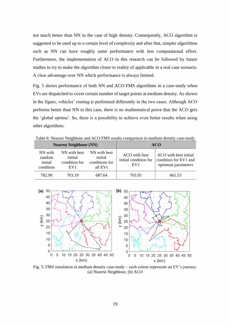
Fig. 5 shows performance of both NN and ACO FMS algorithms in a case-study when

EVs are dispatched to cover certain number of target points at medium density. As shown

in the figure, vehicles’ routing is performed differently in the two cases. Although ACO

performs better than NN in this case, there is no mathematical prove that the ACO gets

the ‘global optima’. So, there is a possibility to achieve even better results when using

other algorithms.

Table 6: Nearest Neighbour and ACO FMS results comparison in medium density case-study

Nearest Neighbour (NN) ACO

NN with

random

initial

condition

NN with best

initial

condition for

EV1

NN with best

initial

conditions for

all EVs

ACO with best

initial condition for

EV1

ACO with best initial

condition for EV1 and

optimum parameters

782.90 703.19 687.64 703.95 661.53

Fig. 5: FMS simulation in medium density case-study – each colour represents an EV’s journey:

(a) Nearest Neighbour, (b) ACO

20

5. Conclusions

In this study, a new algorithm was developed based on ACO for fleet management and

vehicle routing in an optimum way. Nearest-Neighbour algorithm was used as a

benchmark to evaluate performance of the proposed algorithm. The results demonstrated

that the new algorithm is able to improve fleet’s performance 3.8 % in terms of overall

fleet mileage that can lead to a significant save of energy in large scale over time. Even

more achievement is theoretically possible by using other versions of ACO or other

algorithms since there is no mathematical prove that the proposed ACO algorithm gets

the ‘global optima’.

Pheromone concentration was found as the most important aspect to get ACO algorithm

work properly and get the desired performance. Initial pheromone and pheromone

updating together with evaporation, which involve α and ρ parameters, are the main

matters to accomplish the self-learning characteristic of the algorithm and make the best

use of it for a FMS problem. In addition to the ACO parameters, the impacts of the initial

condition and the level of density were investigated. The results demonstrated that initial

condition has a significant effect on ACO FMS algorithm. According to the results, a

combination of random and NN initial conditions can provide the best performance of the

proposed ACO FMS algorithm. The influence of target points’ density was also

investigated by considering three levels of density. The main outcome was that the ACO

algorithm’s performance is restricted when complexity increases. In that case, a

reasonably long time is required to do the optimisation. This cannot be a feasible solution

particularly in an online application.

In this study, a particular FMS case-study was considered in which EV fleet is charged

over night at depot to be ready for operation in the next day. In comparison with literature,

ACO had been already used to perform the Travelling Salesman or Vehicle Routing

problems. However, direct implementation on FMS is what gives novelty to the research.

Combining both research areas is where real application can be done. Regarding recent

battery technology developments and increasing range of EVs, e.g. Nissan LEAF 2018

with 40 kWh battery capacity vs. the older version with 24 kWh, slow overnight charging

can be a feasible solution if the range of EV would be enough for the whole day operation

of the fleet. This would bring benefits like decreasing battery degradation due to fast

21

charging, and also more efficient interaction between EV fleet and the grid. As an

extension of this study, other scenarios can be considered as well. Examples are

considering fast charging during the day or considering more than one depot. Additionally

dynamic behaviour of the environment can be studied, e.g. the E-ACO done by Xu, Pu

and Duan (2018). The multi-depot case-study is categorised as a MTSP. In that case, more

than optimising the position of the depot, which is usually given randomly, the objective

is to show the distribution between depots and customers. A solutions of such a problem

in the literature is Minimum-Maximum MTSP where the aim is to “minimise the

maximum tour length of a single agent instead of minimising the overall sum of tour

lengths by all agents” (Kivelevitch, Cohen, & Kumar, 2012). The proposed FMS

algorithm in this study is designed to work in offline condition however, an online version

of it can be developed in future studies. In that case, the ‘optimisation time’ would be as

important as the objective function that needs proper trade-offs.

References

Abousleiman, R., & Rawashdeh, O. (2014). Energy-efficient routing for electric vehicles using metaheuristic optimization frameworks. 17th IEEE Mediterr. Electrotech. Conf., (pp. 298-304). Cernobbio, Italy.

Barco, J., Guerra, A., Muñoz, L., & Quijano, N. (2017). Optimal Routing and Scheduling of Charge for Electric Vehicles: A Case Study. Mathematical Problems in Engineering, 1-16.

Bell, J. E., & McMullen, P. R. (2004). Ant colony optimization techniques for the vehicle routing problem. Adv. Eng. Informatics, 18(1), 41-48.

Betz, J., Werner, D., & Lienkamp, M. (2016). Fleet Disposition Modeling to Maximize Utilization of Battery Electric Vehicles in Companies with On-Site Energy Generation. Transp. Res. Procedia, 19, 241-257.

Boone, N., Sathyan, A., & Cohen, K. (2015). Enhanced Approaches to Solving the Multiple Traveling Salesman Problem. AIAA Infotech @ Aerosp., 1-7.

Chao, Z. H., & Xiaohong, C. (2013). Optimizing Battery Electric Bus Transit Vehicle Scheduling with Battery Exchanging : Model and Case Study. Procedia - Soc. Behav. Sci., 96, 2725-2736.

Chen, T. D., Kockelman, K. M., & Hanna, J. P. (2016). Operations of a shared , autonomous , electric vehicle fleet : Implications of vehicle & charging infrastructure decisions. Transp. Res. Part A, 94, 243-254.

22

Chen, X., Kong, Y., Fang, X., & Wu, Q. (2011). A fast two-stage ACO algorithm for robotic path planning . Neural Computing and Applications, 22(2), 313-319.

Christofides, N. (1976). The vehicle routing problem. Revue Française a Automatique, Informatique et Recherche Opérationnel, 10(2), 55-70.

Dorigo, M., & Gambardella, L. M. (1997). Ant colonies for the travelling salesman problem. Biosystems, 43(2), 73-81.

Erdoĝan, S., & Miller-Hooks, E. (2012). A Green Vehicle Routing Problem. Transp. Res. Part E Logist. Transp. Rev., 48(1), 100-114.

Fotouhi, A., Auger, D. J., Cleaver, T., Shateri, N., Propp, K., & Longo, S. (2016). Influence of Battery Capacity on Performance of an Electric Vehicle Fleet. 5th Int. Conf. Renew. Energy Res. Appl. Birmingham, UK.

Gaertner, D., & Clark, K. (2005). On Optimal Parameters for Ant Colony Optimization algorithms TSP classifications. International Conference on Artificial Intelligence. Las Vegas, Nevada, USA.

Goel, R. and Maini, R. (2018) ‘A hybrid of ant colony and firefly algorithms ( HAFA ) for solving vehicle routing problems’, Journal of Computational Science, 25 Elsevier B.V., pp. 28–37.

Heris, S. M. (2015, September 4). MATLAB implementation of ACO for Discrete and Combinatorial Optimization Problems. Retrieved June 15, 2018, from https://uk.mathworks.com/matlabcentral/fileexchange/52859-ant-colony-optimization-aco

Hu, J., Morais, H., Sousa, T., & Lind, M. (2016). Electric vehicle fleet management in smart grids : A review of services , optimization and control aspects. Renewable and Sustainable Energy Reviews, 56, 1207-1226.

Jaradat, G. M. (2018). Hybrid elitist-ant system for a symmetric traveling salesman problem: case of Jordan. Neural Computing and Applications, 29(2), 565-578.

Johnson, S. (2001). Emergence: The Connected Lives of Ants, Brains, Cities and Software. Penguin Books.

Kivelevitch, E. H., Cohen, K., & Kumar, M. (2012). A binary programming solution to the Multiple-Depot, Multiple Traveling Salesman Problem with constant profits. AIAA Infotech Aerosp. Conf. Exhib. Garden Grove, CA, USA.

Laporte, G. (1992). The traveling salesman problem: An overview of exact and approximate algorithms. Eur. J. Oper. Res., 59(2), 231-247.

Lin, S. (1965). Computer Solutions of the Traveling Salesman Problem. Bell Syst. Tech. J., 44(10), 2245-2269.

23

Ma, J., Yang, T., Hou, Z.-G., Tan, M., & Liu, D. (2007). Neurodynamic programming: a case study of the traveling salesman problem. Neural Computing and Applications, 17(4), 347-355.

Murakami, K. (2017) ‘A new model and approach to electric and diesel-powered vehicle routing’, Transportation Research Part E, 107 Elsevier Ltd, pp. 23–37.

Narasimha, K. S., & Kumar, M. (2011). Ant Colony Optimization Technique to Solve the Min-Max Single Depot Vehicle Routing Problem. American Control Conference, (pp. 3257-3262). San Francisco, CA, USA.

Ouaarab, A., Ahiod, B., & Yang, X.-S. (2013). Discrete cuckoo search algorithm for the travelling salesman problem. Neural Computing and Applications, 24(7), 1659-1669.

Palmieri, N., Yang, X.-S., Rango, F. D., & Marano, S. (2017). Comparison of bio-inspired algorithms applied to the coordination of mobile robots considering the energy consumption. Neural Computing and Applications, 1-24.

Saji, Y., & Riffi, M. E. (2015). A novel discrete bat algorithm for solving the travelling salesman problem. Neural Computing and Applications, 27(7), 1853-1866.

Schiffer, M., & Walther, G. (2017). The electric location routing problem with time windows and partial recharging. Eur. J. Oper. Res., 260(3), 995-1013.

Tarasewich, P., & McMullen, P. R. (2002). Swarm Intelligence: Power in Numbers. Commun. ACM, 45(8), 62-67.

Xu, H., Pu, P. and Duan, F. (2018) ‘Dynamic Vehicle Routing Problems with Enhanced Ant Colony Optimization’, 2018

Zhang, Q., & Zhang, C. (2018). An improved ant colony optimization algorithm with strengthened pheromone updating mechanism for constraint satisfaction problem. Neural Computing and Applications, 30(10), 3209-3220.

Zhang, S., Gajpal, Y., Appadoo, S.S. and Abdulkader, M.M.S. (2018) ‘Electric Vehicle Routing Problem with Recharging Stations for Minimizing Energy Consumption’, International Journal of Production Economics, Elsevier B.V.