electric power quality - utkweb.eecs.utk.edu/~dcostine/ece620/fall2015/... · power quality metrics...
TRANSCRIPT

' $
& %CURENT & NUCEER Centers, Northeastern University
ELECTRIC POWER QUALITY
Hanoch Lev-Ari
Northeastern University, Boston, MA
and
Aleksandar M. Stankovic
Tufts University, Medford, MA
Sept 9, 2015
' $POWER QUALITY METRICS
& %CURENT & NUCEER Centers, Northeastern University
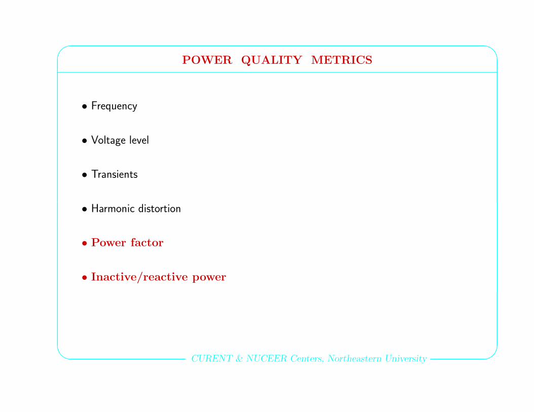
• Frequency
• Voltage level
• Transients
• Harmonic distortion
• Power factor
• Inactive/reactive power
' $HISTORICAL EVOLUTION
& %CURENT & NUCEER Centers, Northeastern University
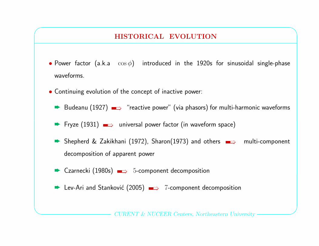
• Power factor (a.k.a cosφ) introduced in the 1920s for sinusoidal single-phase
waveforms.
• Continuing evolution of the concept of inactive power:
è Budeanu (1927) ï “reactive power” (via phasors) for multi-harmonic waveforms
è Fryze (1931) ï universal power factor (in waveform space)
è Shepherd & Zakikhani (1972), Sharon(1973) and others ï multi-component
decomposition of apparent power
è Czarnecki (1980s) ï 5-component decomposition
è Lev-Ari and Stankovic (2005) ï 7-component decomposition

Agreement on Reactive Power
Standard definitions [Buchholz, Schallenberger, Stanley]:
‖V ‖2 =< v v⊤ >0, ‖I‖2 =< i i⊤ >0, S = ‖V ‖‖I‖
P =< i⊤ v >0, Q2 = S2 − P 2, kPF =P
S
Energy Processing Laboratory – p. 4/38
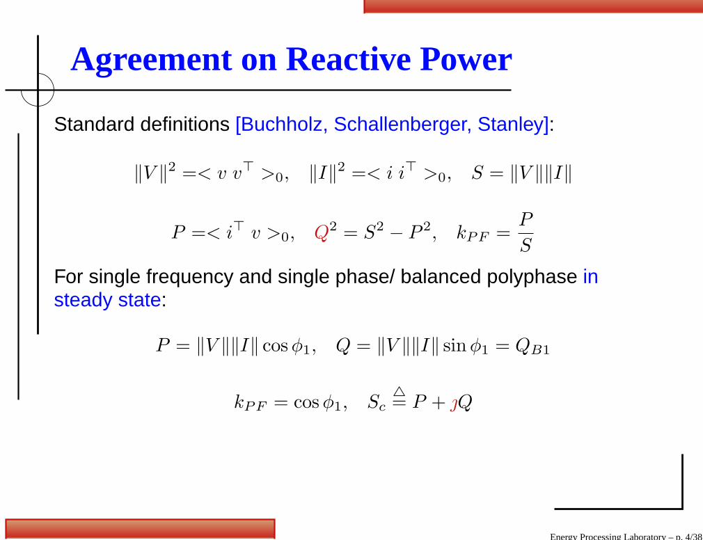
Agreement on Reactive Power
Standard definitions [Buchholz, Schallenberger, Stanley]:
‖V ‖2 =< v v⊤ >0, ‖I‖2 =< i i⊤ >0, S = ‖V ‖‖I‖
P =< i⊤ v >0, Q2 = S2 − P 2, kPF =P
S
For single frequency and single phase/ balanced polyphase insteady state:
P = ‖V ‖‖I‖ cos φ1, Q = ‖V ‖‖I‖ sinφ1 = QB1
kPF = cos φ1, Sc= P + Q
Energy Processing Laboratory – p. 4/38
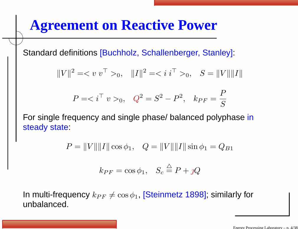
Agreement on Reactive Power
Standard definitions [Buchholz, Schallenberger, Stanley]:
‖V ‖2 =< v v⊤ >0, ‖I‖2 =< i i⊤ >0, S = ‖V ‖‖I‖
P =< i⊤ v >0, Q2 = S2 − P 2, kPF =P
S
For single frequency and single phase/ balanced polyphase insteady state:
P = ‖V ‖‖I‖ cos φ1, Q = ‖V ‖‖I‖ sinφ1 = QB1
kPF = cos φ1, Sc= P + Q
In multi-frequency kPF 6= cos φ1, [Steinmetz 1898]; similarly forunbalanced.
Energy Processing Laboratory – p. 4/38

' $OUTLINE
& %CURENT & NUCEER Centers, Northeastern University
è SINGLE-PHASE SINUSOIDAL WAVEFORMS
• Single-phase non-sinusoidal waveforms
• Euclidean waveform spaces
• Inactive power components
• Polyphase waveforms
• Dynamic power components

' $GENESIS: SINGLE-PHASE SINUSOIDAL WAVEFORMS
& %CURENT & NUCEER Centers, Northeastern University
Waveforms (via rms phasors):
v(t) =√
2<V eωt
ï Vrmsdef=
[1
T
∫ T
0
v2(t) dt
]1/2
= |V |
i(t) =√
2<I eωt
ï Irms = |I |
Instantaneous power:
p(t)def= v(t) i(t) = <V I∗ + <V I e2 ωt (more to come)
Average (“real”) power:
Pdef=
1
T
∫ T
0
p(t) dt = <V I∗
1

' $SINGLE-PHASE SINUSOIDAL WAVEFORMS (2)
& %CURENT & NUCEER Centers, Northeastern University
Power factor:
PFdef=
P
Vrms Irms=
<V I∗|V | |I | = cosφ ≤ 1 (direct manipulation)
where φdef= arg (V/I)
2
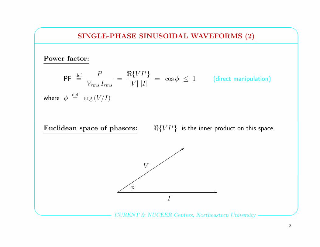
' $SINGLE-PHASE SINUSOIDAL WAVEFORMS (2)
& %CURENT & NUCEER Centers, Northeastern University
Power factor:
PFdef=
P
Vrms Irms=
<V I∗|V | |I | = cosφ ≤ 1 (direct manipulation)
where φdef= arg (V/I)
Euclidean space of phasors: <V I∗ is the inner product on this space
3
V
-
I
φ
2

' $SINGLE-PHASE SINUSOIDAL WAVEFORMS (3)
& %CURENT & NUCEER Centers, Northeastern University
Apparent power:
• When I =V
Rï φ = 0 and P = Vrms Irms
def= S
• In general P ≤ S, and so Irms ≥ P
Vrms
def= IF ï
Excessive power loss in the supply line
• Utility charges extra for imperfect power factor
è Solution – shunt compensator
3

' $SINGLE-PHASE SINUSOIDAL WAVEFORMS (4)
& %CURENT & NUCEER Centers, Northeastern University
Compensation (traditional):
CapacitiveCompensator
InductiveLoad
- -
6
Generator ∼
icomp(t)
is(t) i(t)
v(t)
6
?
Exact compensation (at a single frequency) requires that
=
ωC +1
R + ωL
= 0 ï C =L
|R + ωL|2
4

' $SINGLE-PHASE SINUSOIDAL WAVEFORMS (5)
& %CURENT & NUCEER Centers, Northeastern University
Reactive power:
Qdef= =V I∗ = Vrms Irms sinφ
Complex apparent power:
Sc = P + Q = V I∗ = Vrms Irms e φ
|Sc|2 = P 2 + Q2 ≡ S2
Power quality gap: fully explained by Q (reactive power meters)
Q = 0 ⇐⇒ cosφ = 1
5
' $OUTLINE
& %CURENT & NUCEER Centers, Northeastern University
• Single-phase sinusoidal waveforms
è SINGLE-PHASE NON-SINUSOIDAL WAVEFORMS
• Euclidean waveform spaces
• Inactive power components
• Polyphase waveforms
• Dynamic power components

' $SINGLE-PHASE PERIODIC (NON-SINUSOIDAL) WAVEFORMS
& %CURENT & NUCEER Centers, Northeastern University
Causes for multiple harmonics:
• Load nonlinearity ï multi-harmonic current
• Non-negligible line impedance ï multi-harmonic voltage
• HVDC: Transformers and converters
Metrics of harmonic distortion:
• THD
• Variation of equivalent admittances with respect to harmonic index
Challenges:
How to define Vrms , Irms, P , S, PF, reactive power?
6

' $SINGLE-PHASE PERIODIC (NON-SINUSOIDAL) WAVEFORMS (2)
& %CURENT & NUCEER Centers, Northeastern University
Waveforms:
v(t) =∑
k
√2<Vk e
k ωt
i(t) =∑
k
√2<Ik e
k ωt
V 2rms
def=
1
T
∫ T
0
v2(t) dt =∑
k
|Vk|2 =∑
k
V 2rms,k
I2rms
def=
1
T
∫ T
0
i2(t) dt =∑
k
|Ik|2 =∑
k
I2rms,k
Average power:
Pdef=
1
T
∫ T
0
p(t) dt =1
T
∫ T
0
v(t) i(t) dt =∑
k
<VkI∗k =
∑
k
Pk
7

' $OUTLINE
& %CURENT & NUCEER Centers, Northeastern University
• Single-phase sinusoidal waveforms
• Single-phase nonsinusoidal waveforms
è EUCLIDEAN WAVEFORM SPACES
• Inactive power components
• Polyphase waveforms
• Dynamic power components

' $EUCLIDEAN WAVEFORM SPACES
& %CURENT & NUCEER Centers, Northeastern University
Space elements:
v(t) and i(t) are elements in the space of all T -periodic square-integrable waveforms.
Inner product and norm:
〈〈 x(·) , y(·) 〉〉 def=
1
T
∫
T
x(s) y(s) ds , P = 〈〈 v(·) , i(·) 〉〉
Vrms = ‖v(·)‖ ≡√
〈〈 v(·) , v(·) 〉〉 , Irms = ‖i(·)‖ ≡√
〈〈 i(·) , i(·) 〉〉
8

' $EUCLIDEAN WAVEFORM SPACES
& %CURENT & NUCEER Centers, Northeastern University
Space elements:
v(t) and i(t) are elements in the space of all T -periodic square-integrable waveforms.
Inner product and norm:
〈〈 x(·) , y(·) 〉〉 def=
1
T
∫
T
x(s) y(s) ds , P = 〈〈 v(·) , i(·) 〉〉
Vrms = ‖v(·)‖ ≡√
〈〈 v(·) , v(·) 〉〉 , Irms = ‖i(·)‖ ≡√
〈〈 i(·) , i(·) 〉〉
Orthogonality of harmonics:
1
T
∫ T
0
cos(kωt + θk) cos(`ωt + θ`) dt =
0 k 6= `
12cos (θk − θ`) k = `
8

' $EUCLIDEAN WAVEFORM SPACES (2)
& %CURENT & NUCEER Centers, Northeastern University
Fourier series representation:
x(t) = X0 +
∞∑
k=1
√2<Xk e
kωt , 〈〈 x(·) , y(·) 〉〉 =
∞∑
k=0
<Xk Y∗k
Xkdef=
1T
∫
T
x(t) dt k = 0
√2
T
∫
T
x(t) e−jkωt dt k ≥ 1
(one-sided rms phasors)
9

' $EUCLIDEAN WAVEFORM SPACES (2)
& %CURENT & NUCEER Centers, Northeastern University
Fourier series representation:
x(t) = X0 +
∞∑
k=1
√2<Xk e
kωt , 〈〈 x(·) , y(·) 〉〉 =
∞∑
k=0
<Xk Y∗k
Xkdef=
1T
∫
T
x(t) dt k = 0
√2
T
∫
T
x(t) e−jkωt dt k ≥ 1
(one-sided rms phasors)
Voltage and current waveforms: (without DC component)
P = 〈〈 v(·) , i(·) 〉〉 =∞∑
k=1
<Vk I∗k
V 2rms ≡ ‖v(·)‖2 =
∞∑
k=1
|Vk|2 , I2rms ≡ ‖i(·)‖2 =
∞∑
k=1
|Ik|2
9

' $EUCLIDEAN WAVEFORM SPACES (3)
& %CURENT & NUCEER Centers, Northeastern University
Dimension:
• Sinusoidal waveforms: dimension = 2
e1(t) =√
2 cosωt , e2(t) =√
2 sinωt
• L-harmonic waveforms: dimension = 2L (no DC component)
(√
2 cos kωt ,√
2 sin kωt) ; 1 ≤ k ≤ L
• Arbitrary periodic waveforms: dimension = ∞ (Hilbert space)
è L-harmonic basis with L = ∞.
10

' $EUCLIDEAN WAVEFORM SPACES (4)
& %CURENT & NUCEER Centers, Northeastern University
Historical footnote:
• Stanis law Fryze (1885-1964), Professor at the Lwow Polytechnic (then in Poland,
now in the Ukraine), originated in 1932 the function-analytic interpretation of power
system waveforms.
• A contemporary of Fryze at the Lwow Polytechnic (and, apparently, a professional
colleague) was . . .
11

' $EUCLIDEAN WAVEFORM SPACES (4)
& %CURENT & NUCEER Centers, Northeastern University
Historical footnote:
• Stanis law Fryze (1885-1964), Professor at the Lwow Polytechnic (then in Poland,
now in the Ukraine), originated in 1932 the function-analytic interpretation of power
system waveforms.
• A contemporary of Fryze at the Lwow Polytechnic (and, apparently, a professional
colleague) was Stefan Banach (1892-1945).
11

Introduction
A history flashback
PioneersGetting basics right - Buchholz, Schallenberger, StanleyA trouble in paradise - multiple harmonics Steinmetz 1898
National schools - glowne nurty
Romania: A.D. Iliovici (1925), C. Busila, C. Budeanu, I. Antoniu (1950),F. Manea, V. Nedelcu (1960) M. Milic (1970), A. Tugulea, A. Emanuel,Poland: S. Fryze, M. Erlicki (1950), Z. Nowomiejski (1980), L.Czarnecki,Germany: F. Buchholz (1920), W. Quade (1930), R. Richter (1930), M.Depenbrock (1970), H. Fisher (1980).
Alex Stankovic (Alvin H Howell Professor) Sparse Sampling Lagow Seminar 9 / 47
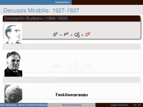
Introduction
Decussis Mirabilis: 1927-1937Constantin Budeanu (1886-1959)
S2 = P2 + Q2B + D2
Stanislaw Fryze (1885-1964)
ia(t) =< i v> >< v v> >
v(t)
Wilhelm Quade (1898-1975)
Alex Stankovic (Alvin H Howell Professor) Sparse Sampling Lagow Seminar 10 / 47

Introduction
Decussis Mirabilis: 1927-1937Constantin Budeanu (1886-1959)
S2 = P2 + Q2B + D2
Stanislaw Fryze (1885-1964)
ia(t) =< i v> >< v v> >
v(t)
Wilhelm Quade (1898-1975)
Alex Stankovic (Alvin H Howell Professor) Sparse Sampling Lagow Seminar 10 / 47

Introduction
Decussis Mirabilis: 1927-1937Constantin Budeanu (1886-1959)
S2 = P2 + Q2B + D2
Stanislaw Fryze (1885-1964)
ia(t) =< i v> >< v v> >
v(t)
Wilhelm Quade (1898-1975)
Alex Stankovic (Alvin H Howell Professor) Sparse Sampling Lagow Seminar 10 / 47

Reactive Power - Schools
Romania: A.D. Iliovici (1925), C. Busila, C. Budeanu, I.Antoniu (1950), F. Manea, V. Nedelcu (1960) M. Milic (1970),A. Tugulea, A. Emanuel,
Poland: S. Fryze, M. Erlicki (1950), Z. Nowomiejski (1980), L.Czarnecki,
Germany: F. Buchholz (1920), W. Quade (1930), R. Richter(1930), M. Depenbrock (1970), H. Fisher (1980).
Energy Processing Laboratory – p. 20/38

' $EUCLIDEAN WAVEFORM SPACES (5)
& %CURENT & NUCEER Centers, Northeastern University
Power factor:
PFdef=
P
Vrms Irms=
〈〈 v(·) , i(·) 〉〉‖v(·)‖ ‖i(·)‖ = cosψ ≤ 1
where ψ is the angle between voltage and current in the waveform space.
3
v(·)
-
i(·)ψ
PF = 1 ⇐⇒ ψ = 0 ⇐⇒ P = S ⇐⇒ i(t) =v(t)
R
12
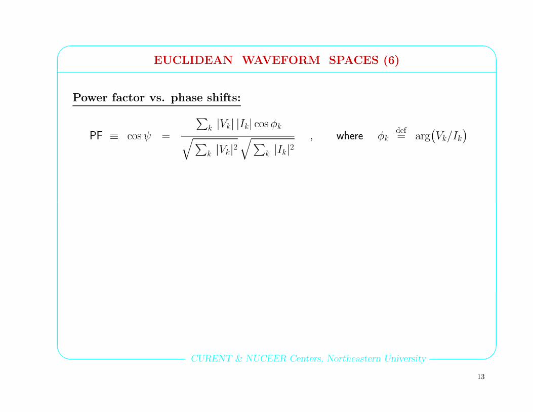
' $EUCLIDEAN WAVEFORM SPACES (6)
& %CURENT & NUCEER Centers, Northeastern University
Power factor vs. phase shifts:
PF ≡ cosψ =
∑
k |Vk| |Ik| cosφk
√∑
k |Vk|2√∑
k |Ik|2, where φk
def= arg
(Vk/Ik
)
13

' $EUCLIDEAN WAVEFORM SPACES (6)
& %CURENT & NUCEER Centers, Northeastern University
Power factor vs. phase shifts:
PF ≡ cosψ =
∑
k |Vk| |Ik| cosφk
√∑
k |Vk|2√∑
k |Ik|2, where φk
def= arg
(Vk/Ik
)
Warning:
φk = 0 for all k ï P < S (in general)
because in this case
PF =
∑
k |Vk| |Ik|√∑
k |Vk|2√∑
k |Ik|2< 1 (why?)
The guilty party: Distortion power (D)
13
' $OUTLINE
& %CURENT & NUCEER Centers, Northeastern University
• Single-phase sinusoidal waveforms
• Single-phase nonsinusoidal waveforms
• Euclidean waveform spaces
è INACTIVE POWER COMPONENTS
• Polyphase waveforms
• Dynamic power components

' $A MENAGERIE OF INACTIVE POWER COMPONENTS
& %CURENT & NUCEER Centers, Northeastern University
Budeanu reactive power: (Why ”reactive”? Why ”Budeanu”?)
QBdef=
∑
k
=Vk I∗k =
∑
k
|Vk| |Ik| sinφk
QB = 0 when φk = 0 for all k (but it can also vanish when φk 6= 0)
14

' $A MENAGERIE OF INACTIVE POWER COMPONENTS
& %CURENT & NUCEER Centers, Northeastern University
Budeanu reactive power: (Why ”reactive”? Why ”Budeanu”?)
QBdef=
∑
k
=Vk I∗k =
∑
k
|Vk| |Ik| sinφk
QB = 0 when φk = 0 for all k (but it can also vanish when φk 6= 0)
Distortion power: (Budeanu, 1927)
In general, (details on next page)
P 2 +Q2B =
∣∣∣
∑
k
Vk I∗k
∣∣∣
2
< S2
so let’s define
Ddef=
√
S2 − (P 2 +Q2B)
A purely arithmetical (unsigned) definition, with no physical meaning.
14

' $A MENAGERIE OF INACTIVE POWER COMPONENTS (2)
& %CURENT & NUCEER Centers, Northeastern University
Power quality gap:
P 2 +Q2B =
[
<∑
k
Vk I∗k
]2
+[
=∑
k
Vk I∗k
]2
=∣∣∣
∑
k
Vk I∗k
∣∣∣
2
and (using Cauchy-Schwarz inequality for complex vectors)
∣∣∣
∑
k
Vk I∗k
∣∣∣
2
≤(∑
k
|Vk|2) (
∑
k
|Ik|2)
≡ S2
P 2 +Q2B ≤ S2
ï D ≥ 0 (terminus for Budeanu)
15
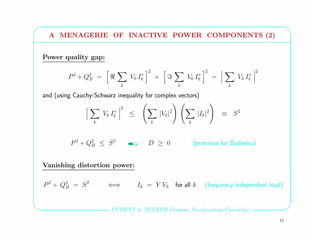
' $A MENAGERIE OF INACTIVE POWER COMPONENTS (2)
& %CURENT & NUCEER Centers, Northeastern University
Power quality gap:
P 2 +Q2B =
[
<∑
k
Vk I∗k
]2
+[
=∑
k
Vk I∗k
]2
=∣∣∣
∑
k
Vk I∗k
∣∣∣
2
and (using Cauchy-Schwarz inequality for complex vectors)
∣∣∣
∑
k
Vk I∗k
∣∣∣
2
≤(∑
k
|Vk|2) (
∑
k
|Ik|2)
≡ S2
P 2 +Q2B ≤ S2
ï D ≥ 0 (terminus for Budeanu)
Vanishing distortion power:
P 2 + Q2B = S2 ⇐⇒ Ik = Y Vk for all k (frequency-independent load)
15

' $A MENAGERIE OF INACTIVE POWER COMPONENTS (3)
& %CURENT & NUCEER Centers, Northeastern University
Equivalent load admittances: Var Yk > 0 ⇐⇒ D > 0
Ykdef=
IkVk
= gk − bk (Why I/V ? What if Vk = 0?)
(How about nonlinear loads?)
16

' $A MENAGERIE OF INACTIVE POWER COMPONENTS (3)
& %CURENT & NUCEER Centers, Northeastern University
Equivalent load admittances: Var Yk > 0 ⇐⇒ D > 0
Ykdef=
IkVk
= gk − bk (Why I/V ? What if Vk = 0?)
(How about nonlinear loads?)
Weighted mean expressions:
P =∑
k <Vk I∗k =
∑
k gk |Vk|2 ∼ weighted mean of gk
QB =∑
k =Vk I∗k =
∑
k bk |Vk|2 ∼ weighted mean of bk
16

' $A STATISTICAL (SPREAD) PERSPECTIVE
& %CURENT & NUCEER Centers, Northeastern University
Weights: wkdef=
|Vk|2
V 2rms
(∑
k wk = 1)
(Why?)
Weighted means:
µgdef=
∑
k wk gk =P
V 2rms
µbdef=
∑
k wk bk =QB
V 2rms
ï P 2 + Q2B = V 4
rms
(
µ2g + µ2
b
)
17

' $A STATISTICAL (SPREAD) PERSPECTIVE
& %CURENT & NUCEER Centers, Northeastern University
Weights: wkdef=
|Vk|2
V 2rms
(∑
k wk = 1)
(Why?)
Weighted means:
µgdef=
∑
k wk gk =P
V 2rms
µbdef=
∑
k wk bk =QB
V 2rms
ï P 2 + Q2B = V 4
rms
(
µ2g + µ2
b
)
Weighted variances: D = 0 ⇐⇒ σ2g = 0 = σ2
b
σ2g
def=
∑
k wk
(gk − µg
)2
σ2b
def=
∑
k wk
(bk − µg
)2
17
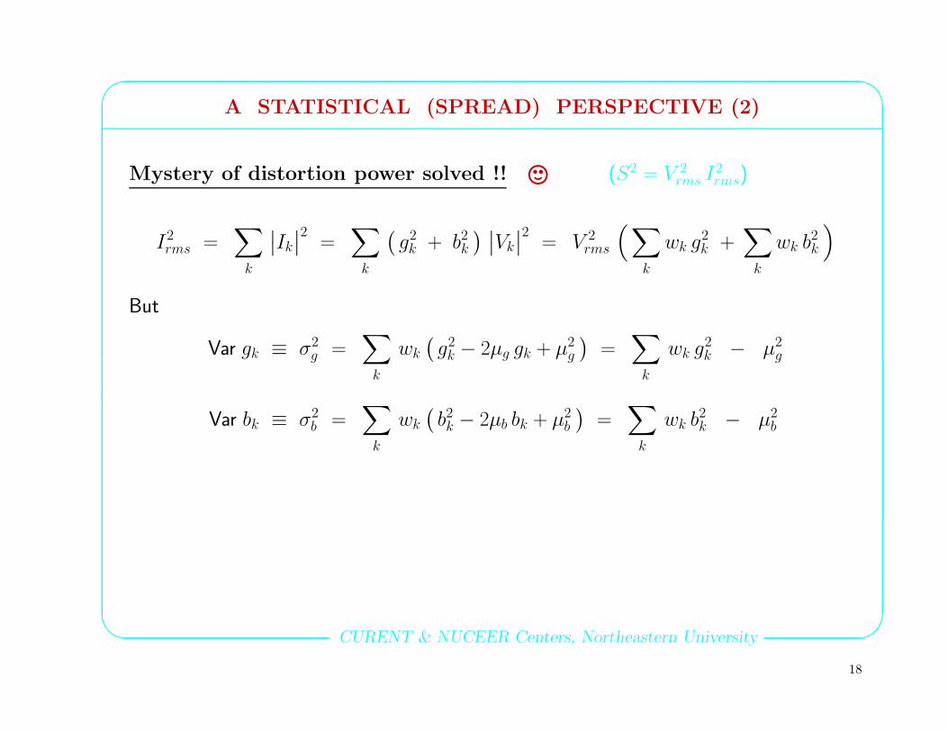
' $A STATISTICAL (SPREAD) PERSPECTIVE (2)
& %CURENT & NUCEER Centers, Northeastern University
Mystery of distortion power solved !! , (S2 = V 2rms I
2rms)
I2rms =
∑
k
∣∣Ik∣∣2
=∑
k
(g2
k + b2k) ∣∣Vk
∣∣2
= V 2rms
(∑
k
wk g2k +
∑
k
wk b2k
)
But
Var gk ≡ σ2g =
∑
k
wk
(g2
k − 2µg gk + µ2g
)=∑
k
wk g2k − µ2
g
Var bk ≡ σ2b =
∑
k
wk
(b2k − 2µb bk + µ2
b
)=∑
k
wk b2k − µ2
b
18

' $A STATISTICAL (SPREAD) PERSPECTIVE (2)
& %CURENT & NUCEER Centers, Northeastern University
Mystery of distortion power solved !! , (S2 = V 2rms I
2rms)
I2rms =
∑
k
∣∣Ik∣∣2
=∑
k
(g2
k + b2k) ∣∣Vk
∣∣2
= V 2rms
(∑
k
wk g2k +
∑
k
wk b2k
)
But
Var gk ≡ σ2g =
∑
k
wk
(g2
k − 2µg gk + µ2g
)=∑
k
wk g2k − µ2
g
Var bk ≡ σ2b =
∑
k
wk
(b2k − 2µb bk + µ2
b
)=∑
k
wk b2k − µ2
b
So
∑
k g2k
∣∣Vk
∣∣2
= V 2rms
[
µ2g + σ2
g
]
∑
k b2k
∣∣Vk
∣∣2
= V 2rms
[
µ2b + σ2
b
]
ï I2rms = V 2
rms
[
µ2g + σ2
g + µ2b + σ2
b
]
18

' $A STATISTICAL (SPREAD) PERSPECTIVE (3)
& %CURENT & NUCEER Centers, Northeastern University
Four-component decomposition:
S2 ≡ V 2rms I
2rms = V 4
rms
[
µ2g + µ2
b + σ2g + σ2
b
]
= P 2 + Q2B + N2
g + N2b
︸ ︷︷ ︸
D2
where
P 2 = V 4rms µ
2g , Q2
B = V 4rms µ
2b
N2g
def= V 4
rms σ2g , N2
bdef= V 4
rms σ2b
so that
D2 = V 4rms
(
σ2g + σ2
b
)
19

' $A STATISTICAL (SPREAD) PERSPECTIVE (4)
& %CURENT & NUCEER Centers, Northeastern University
Out-of-band current: (What if Vk = 0?)
Ωvdef= k ;
|Vk|Vrms
> ε (include only non-negligible harmonics)
I2rms =
∑
k∈Ωv
g2k
∣∣Vk
∣∣2
+∑
k∈Ωv
b2k∣∣Vk
∣∣2
+∑
k 6=Ωv
∣∣Ik∣∣2
20

' $A STATISTICAL (SPREAD) PERSPECTIVE (4)
& %CURENT & NUCEER Centers, Northeastern University
Out-of-band current: (What if Vk = 0?)
Ωvdef= k ;
|Vk|Vrms
> ε (include only non-negligible harmonics)
I2rms =
∑
k∈Ωv
g2k
∣∣Vk
∣∣2
+∑
k∈Ωv
b2k∣∣Vk
∣∣2
+∑
k 6=Ωv
∣∣Ik∣∣2
Five-component decomposition:
S2 ≡ V 2rms I
2rms = P 2 + Q2
B + N2g + N2
b + S2⊥
︸ ︷︷ ︸
D2
where
S2⊥
def= V 2
rms
( ∑
k 6=Ωv
∣∣Ik∣∣2)
20
' $OUTLINE
& %CURENT & NUCEER Centers, Northeastern University
• Single-phase sinusoidal waveforms
• Single-phase nonsinusoidal waveforms
• Euclidean waveform spaces
• Inactive power components
è POLYPHASE WAVEFORMS
• Dynamic power components

' $POLYPHASE CURRENT AND VOLTAGE WAVEFORMS
& %CURENT & NUCEER Centers, Northeastern University
Source
Load
1
2
m
m+1
···
6
v1(t)
6
v2(t)
-i1(t)
-
i2(t)
-im(t)
∑
p
ip(t)
v(t)def=
[v1(t) v2(t) . . . vm(t)
]
i(t)def=
[i1(t) i2(t) . . . im(t)
]
21

' $EUCLIDEAN/HILBERT WAVEFORM SPACES
& %CURENT & NUCEER Centers, Northeastern University
Space elements: real-valued T -periodic square-integrable polyphase waveforms
x(t) =[
x1(t) x2(t) . . . xm(t)]
(row vector)
Inner product and norm:
〈〈 x , y 〉〉 def= 1
T
∫
T
x(t) y>(t) dt ‖ x ‖ def=√
〈〈 x , x 〉〉
Vrms = ‖v(·)‖ , Irms = ‖i(·)‖ , P = 〈〈 v(·) , i(·) 〉〉
Additivity over phases:
V 2rms =
m∑
p=1
V 2rms,p , I2
rms =
m∑
p=1
I2rms,p , P =
m∑
p=1
Pp
22

' $EUCLIDEAN/HILBERT WAVEFORM SPACES (2)
& %CURENT & NUCEER Centers, Northeastern University
Fourier series representation:
x(t) = X0 +
∞∑
k=1
√2<Xk e
kωt (one-sided rms phasors)
Xkdef=
1T
∫
T
x(t) dt k = 0
√2
T
∫
T
x(t) e−jkωt dt k ≥ 1
(row vector)
Parseval identity: ( ↓ one reason for row vectors)
〈〈 x(·) , y(·) 〉〉 =
∞∑
k=0
<Xk YHk =
m∑
p=1
∞∑
k=0
<
X(p)k [Y
(p)k ]∗
X(p)k = p-th element of Xk .
23

' $SINUSOIDAL POLYPHASE WAVEFORMS
& %CURENT & NUCEER Centers, Northeastern University
Equivalent load admittances: (only fundamental harmonic)
Ypdef=
IpVp
= gp − bp(gp and bp now represent spread over phases
)
Four-component power decomposition:
S2 ≡ V 2rms I
2rms = V 4
rms
[
µ2g + σ2
g + µ2b + σ2
b
]
= P 2 + N2g + Q2
B + N2b
where
µg , σ2g = weighted mean and variance of the sequence
gp
µb , σ2b = weighted mean and variance of the sequence
bp
24

' $SINUSOIDAL POLYPHASE WAVEFORMS (2)
& %CURENT & NUCEER Centers, Northeastern University
Example 1: balanced unit voltage, R = 1 = ωL = 1/ωC
g1 = 1 , b1 = 0 ï φ1 = 0
g2 = 0 , b2 = −1 ï φ2 = 90
g3 = 0 , b3 = 1 ï φ3 = −90
R
ωL
1
ωC
1
2
3
0
Power components:
S = 3 , P = 1 , QB = 0 , Ng =√
2 , Nb =√
6 ï PF =1
3
25
' $SINUSOIDAL POLYPHASE WAVEFORMS (3)
& %CURENT & NUCEER Centers, Northeastern University
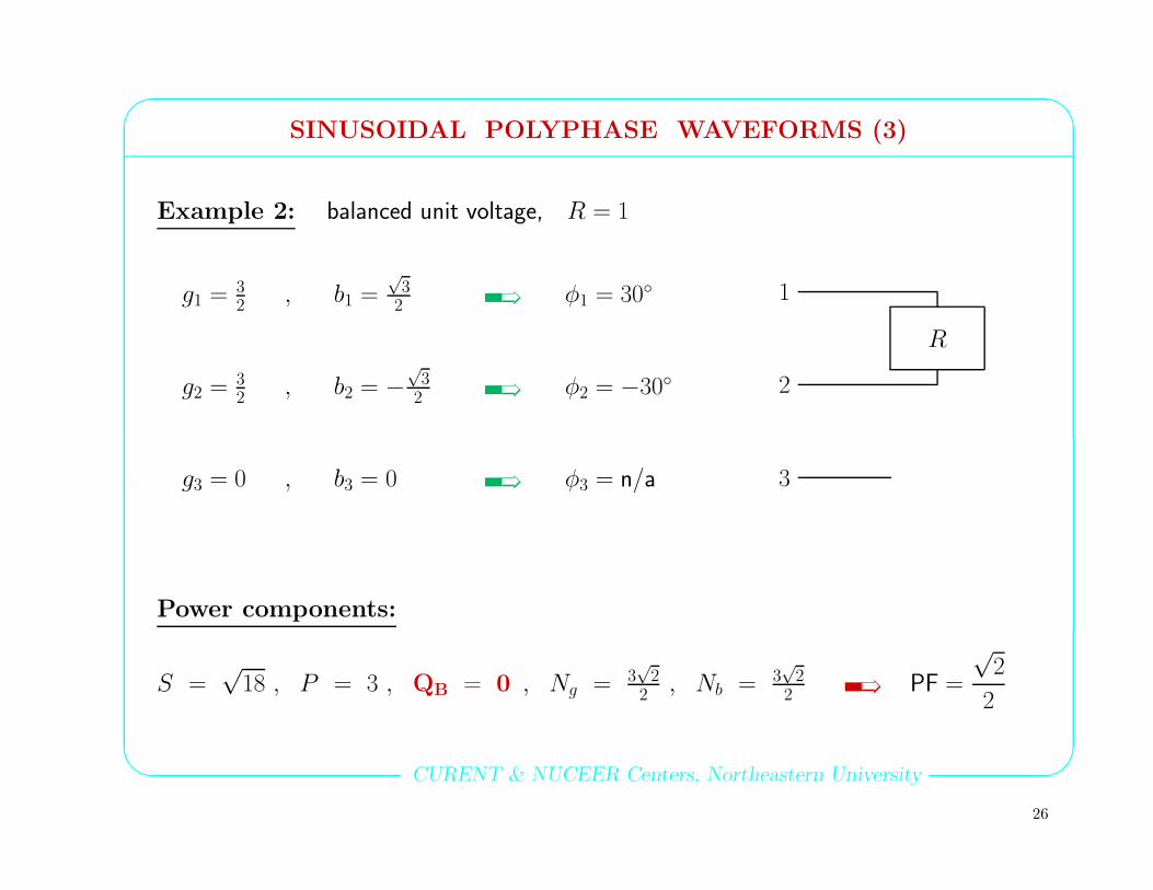
Example 2: balanced unit voltage, R = 1
g1 = 32
, b1 =√
32 ï φ1 = 30
g2 = 32
, b2 = −√
32 ï φ2 = −30
g3 = 0 , b3 = 0 ï φ3 = n/a
R
1
2
3
Power components:
S =√
18 , P = 3 , QB = 0 , Ng = 3√
22, Nb = 3
√2
2 ï PF =
√2
2
26

' $SINUSOIDAL POLYPHASE WAVEFORMS (4)
& %CURENT & NUCEER Centers, Northeastern University
Balanced voltage and current: (“standard” conditions, only positive sequence)
Y1 = Y2 = Y3 ï gp = g and bp = b for all p
Also
φ1 = φ2 = φ3def= φ
27

' $SINUSOIDAL POLYPHASE WAVEFORMS (4)
& %CURENT & NUCEER Centers, Northeastern University
Balanced voltage and current: (“standard” conditions, only positive sequence)
Y1 = Y2 = Y3 ï gp = g and bp = b for all p
Also
φ1 = φ2 = φ3def= φ
Power components:
Ng = 0 = Nb ï S2 = P 2 + Q2B
and
PF ≡ cosψ = cosφ
Indistinguishable from single-phase sinusoidal case.
27
' $NON-SINUSOIDAL POLYPHASE WAVEFORMS
& %CURENT & NUCEER Centers, Northeastern University
Equivalent load admittances:
Y(p)k
def=
I(p)k
V(p)k
= g(p)k − b
(p)k
(k is harmonic index, p is phase index
)
Seven-component power decomposition: (ANOVA: groups = harmonics)
S2 ≡ V 2rms I
2rms = V 4
rms
[
µ2g + σ2
gs + σ2gu
︸ ︷︷ ︸
σ2g
+ µ2b + σ2
bs + σ2bu
︸ ︷︷ ︸
σ2
b
]
+ S2⊥
= P 2 + N2gs + N2
gu + Q2B + N2
bs + N2bu + S2
⊥
where (”u” = within, ”s” = between)
µg , σ2g = weighted mean and variance of the “2D” sequence
g
(p)k
µb , σ2b = weighted mean and variance of the “2D” sequence
b(p)k
28

' $NON-SINUSOIDAL POLYPHASE WAVEFORMS (2)
& %CURENT & NUCEER Centers, Northeastern University
Variance components:
µg(k)def=
∑
p
g(p)k
|V (p)k |2
∑
i |V (i)k |2
, µb(k)def=
∑
p
b(p)k
|V (p)k |2
∑
i |V (i)k |2
σ2gu
def=
∑
k
(∑
p
[g
(p)k − µg(k)
]2 |V (p)k |2V 2
rms
)
(within)
σ2gs
def=
∑
k
(∑
p
[µg(k) − µg
]2 |V (p)k |2V 2
rms
)
(between)
σ2bu
def=
∑
k
(∑
p
[b(p)k − µb(k)
]2 |V (p)k |2V 2
rms
)
(within)
σ2bs
def=
∑
k
(∑
p
[µb(k) − µb
]2 |V (p)k |2V 2
rms
)
(between)
29
' $OUTLINE
& %CURENT & NUCEER Centers, Northeastern University
• Single-phase sinusoidal waveforms
• Single-phase nonsinusoidal waveforms
• Euclidean waveform spaces
• Inactive power components
• Polyphase waveforms
è DYNAMIC POWER COMPONENTS

' $DYNAMIC POWER COMPONENTS
& %CURENT & NUCEER Centers, Northeastern University
Time-variant inner product and norm:
〈〈 x(·) , y(·) 〉〉(t) def= 1
T
∫ t
t−T
x(t) y>(t) dt , ‖x(·)‖(t)def=√
〈〈 x(·) , x(·) 〉〉(t)
Vrms(t) = ‖v(·)‖(t) , Irms(t) = ‖i(·)‖(t) , P (t) = 〈〈 v(·) , i(·) 〉〉(t)
30
' $DYNAMIC POWER COMPONENTS
& %CURENT & NUCEER Centers, Northeastern University
Time-variant inner product and norm:
〈〈 x(·) , y(·) 〉〉(t) def= 1
T
∫ t
t−T
x(t) y>(t) dt , ‖x(·)‖(t)def=√
〈〈 x(·) , x(·) 〉〉(t)
Vrms(t) = ‖v(·)‖(t) , Irms(t) = ‖i(·)‖(t) , P (t) = 〈〈 v(·) , i(·) 〉〉(t)
Dynamic 7-component approach: (transient conditions)
S2(t) ≡ V 2rms(t) I
2rms(t)
= P 2(t) + N2gs(t) + N2
gu(t) + Q2B(t) + N2
bs(t) + N2bu(t) + S2
⊥(t)
è Time-invariant for periodic waveforms
30

A Simple Example
Consider a simple RL circuit (R=0.1, L=0.002) with a sin excitation(V=10), at 60Hz
0 0.01 0.02 0.03 0.04 0.05 0.06 0.07 0.08 0.09 0.1−15
−10
−5
0
5
10
15
20
25
Time
Curre
nt, A
Energy Processing Laboratory – p. 26/38

A Simple Example (2)
The dynamic phasors (according to our definition)
0 0.01 0.02 0.03 0.04 0.05 0.06 0.07 0.08 0.09 0.1−15
−10
−5
0
5
10
15
20
25
Time
Cur
rent
, A
DC
Re
Im
Energy Processing Laboratory – p. 27/38

Reactive Power in the Example
Our inductor example
0 0.02 0.04 0.06 0.08 0.10
10
20
30
40
50
60
70
80
90
100
Time
Pow
er
P
Q
S
QB1
Energy Processing Laboratory – p. 29/38

' $DYNAMIC POWER COMPONENTS (2)
& %CURENT & NUCEER Centers, Northeastern University
Industrial example:
• Power flow during a fault (sag): data collected from a large paper mill.
• Sampling rate is 140 samples/cycle: sufficient to cover multiple harmonics.
• Figures show ten cycles before the fault, and ten cycles after the fault.
31

' $DYNAMIC POWER COMPONENTS (2)
& %CURENT & NUCEER Centers, Northeastern University
Industrial example:
• Power flow during a fault (sag): data collected from a large paper mill.
• Sampling rate is 140 samples/cycle: sufficient to cover multiple harmonics.
• Figures show ten cycles before the fault, and ten cycles after the fault.
• Noticeable current distortion even before the fault: significant values of Ngs and Nbs
• Fault causes significant increase in load imbalance: Ngu and Nbu increase by
(approximately) a factor of 4 during the transient.
31
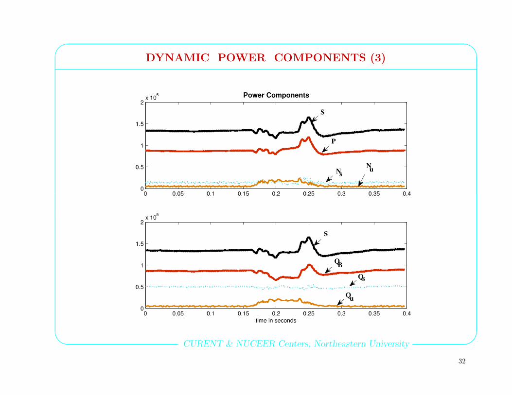
' $DYNAMIC POWER COMPONENTS (3)
& %CURENT & NUCEER Centers, Northeastern University
0 0.05 0.1 0.15 0.2 0.25 0.3 0.35 0.40
0.5
1
1.5
2x 10
5 Power Components
0 0.05 0.1 0.15 0.2 0.25 0.3 0.35 0.40
0.5
1
1.5
2x 10
5
time in seconds
s
S
B
S
N u
Q
N
P
s
Q
Q
u
32
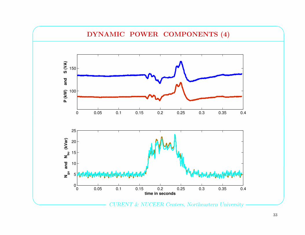
' $DYNAMIC POWER COMPONENTS (4)
& %CURENT & NUCEER Centers, Northeastern University
0 0.05 0.1 0.15 0.2 0.25 0.3 0.35 0.4
100
150P
(k
W)
a
nd
S (
VA
)
0 0.05 0.1 0.15 0.2 0.25 0.3 0.35 0.40
5
10
15
20
25
time in seconds
Ng
u
an
d
Nb
u
(kV
ar)
33

' $INSTANTANEOUS DYNAMIC POWER COMPONENTS
& %CURENT & NUCEER Centers, Northeastern University
Source
Load
1
2
m
m+1
···
6
v1(t)
6
v2(t)
-i1(t)
-
i2(t)
-im(t)
∑
p
ip(t)
v(t)def=
[v1(t) v2(t) . . . vm(t)
]∈ R
m
i(t)def=
[i1(t) i2(t) . . . im(t)
]∈ R
m
34

' $INSTANTANEOUS DYNAMIC POWER COMPONENTS (2)
& %CURENT & NUCEER Centers, Northeastern University
Instantaneous real and apparent power: (Akagi & Nabae approach)
p(t) = v(t) i>(t) , s(t)def=
√[v(t)v>(t)
] [i(t)i>(t)
]
Notice: s2(t) − p2(t) = 0 for single-phase systems.
35

' $INSTANTANEOUS DYNAMIC POWER COMPONENTS (2)
& %CURENT & NUCEER Centers, Northeastern University
Instantaneous real and apparent power: (Akagi & Nabae approach)
p(t) = v(t) i>(t) , s(t)def=
√[v(t)v>(t)
] [i(t)i>(t)
]
Notice: s2(t) − p2(t) = 0 for single-phase systems.
Lagrange identity:
s2(t) − p2(t) =∑
k<`
q2k`(t) = 1
2
∥∥∥Q(t)
∥∥∥
2
F
where (skew-symmetric matrix)
Q(t)def= i>(t) v(t) − v>(t) i(t) =
[
qk`(t)]
k,`=1:m
35

' $THREE PHASE SYSTEMS
& %CURENT & NUCEER Centers, Northeastern University
v(t) =[va(t) vb(t) vc(t)
]
i(t) =[ia(t) ib(t) ic(t)
]
ï qab(t), qbc(t), qac(t)
Coordinate transform: any orthogonal matrix M
[vα(t) vβ(t) vc0)
]=[va(t) vb(t) vc(t)
]M
[iα(t) iβ(t) ic0)
]=[ia(t) ib(t) ic(t)
]M
ï qαβ(t), qαo(t), qβo(t)
36

' $THREE PHASE SYSTEMS
& %CURENT & NUCEER Centers, Northeastern University
v(t) =[va(t) vb(t) vc(t)
]
i(t) =[ia(t) ib(t) ic(t)
]
ï qab(t), qbc(t), qac(t)
Park transform:
[vα(t) vβ(t) vc0)
]=[va(t) vb(t) vc(t)
]M
[iα(t) iβ(t) ic0)
]=[ia(t) ib(t) ic(t)
]M
ï qαβ(t), qαo(t), qβo(t)
where
M =1√3
√2 0 1
−√
22
√6
21
−√
22
−√
62
1
instantaneous “equivalent” of
symmetric sequence components
Special case: vanishing zero-sequence components
vo(t) = 0 = io(t) ï qαo(t) = 0 = qβo(t) , qαβ(t)def= qAN(t)
36

' $THREE PHASE SYSTEMS (2)
& %CURENT & NUCEER Centers, Northeastern University
Interpretations:
• Vanishing zero-sequence (Akagi-Nabae) – when v0(t) = 0 = i0(t) there is only
one non-zero (signed) reactive power quantity qAN(t), which can be conveniently
expressed in terms of the Park transform.
• Vector Calculus Approach (Dai, Liu and Gretsch, 2004) – these three reactive
power quantities can be viewed as the elements of a cross product between the current
and voltage vectors.
37

' $THREE PHASE SYSTEMS (2)
& %CURENT & NUCEER Centers, Northeastern University
Interpretations:
• Vanishing zero-sequence (Akagi-Nabae) – when v0(t) = 0 = i0(t) there is only
one non-zero (signed) reactive power quantity qAN(t), which can be conveniently
expressed in terms of the Park transform.
• Vector Calculus Approach (Dai, Liu and Gretsch, 2004) – these three reactive
power quantities can be viewed as the elements of a cross product between the current
and voltage vectors.
Warnings:
• Both interpretations fail when m > 3. Vectors, such a v(t) and i(t) consist of
m elements, but there are m(m−1)2
distinct instantaneous reactive power quantities.
• Instantaneous powers are “noisy” – hence poor indicators of power events.
37

' $THREE PHASE SYSTEMS (3)
& %CURENT & NUCEER Centers, Northeastern University
0 0.05 0.1 0.15 0.2 0.25 0.3 0.35 0.40
50
100
150
200
time (sec)
p(t
) (
KW
)
0 0.05 0.1 0.15 0.2 0.25 0.3 0.35 0.4−50
0
50
100
150
200
time (sec)
qA
N(t
) (
KV
AR
)
0 0.05 0.1 0.15 0.2 0.25 0.3 0.35 0.40
50
100
150
200
250
time (sec)
s(t
) (
KV
A)
38

' $THREE PHASE SYSTEMS (4)
& %CURENT & NUCEER Centers, Northeastern University
Observations:
• The transient is noticeable in all three waveforms: s(t), p(t) and qAN(t).
• Duration of transient is not easily discernible from either one.
• We get no information about the nature of the fault.
39

' $THREE PHASE SYSTEMS (5)
& %CURENT & NUCEER Centers, Northeastern University
0 0.05 0.1 0.15 0.2 0.25 0.3 0.35 0.4−20
0
20
40
60
80
100
120
140
160
180
time (sec)
qA
N(t
) (
KV
AR
)
40
Sub-cycle
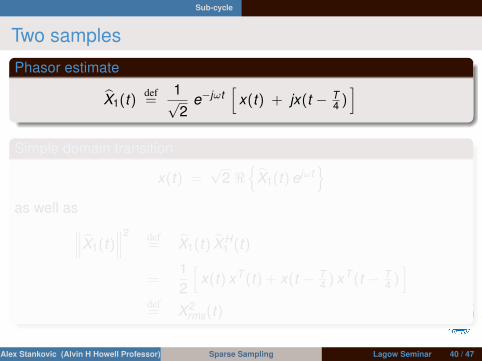
Two samples
Phasor estimate
X1(t)def=
1√2
e−jωt[
x(t) + jx(t − T4 )]
Simple domain transition
x(t) =√
2 <
X1(t)ejωt
as well as∥∥∥X1(t)∥∥∥2 def
= X1(t) X H1 (t)
=12
[x(t) xT (t) + x(t − T
4 ) xT (t − T4 )]
def= X 2
rms(t)
Alex Stankovic (Alvin H Howell Professor) Sparse Sampling Lagow Seminar 40 / 47

Sub-cycle
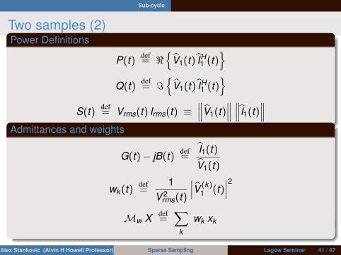
Two samples (2)Power Definitions
P(t) def= <
V1(t) IH
1 (t)
Q(t) def= =
V1(t) IH
1 (t)
S(t) def= Vrms(t) Irms(t) ≡
∥∥∥V1(t)∥∥∥ ∥∥∥I1(t)
∥∥∥Admittances and weights
G(t)− jB(t) def=
I1(t)
V1(t)
wk (t)def=
1V 2
rms(t)
∣∣∣V (k)1 (t)
∣∣∣2Mw X def
=∑
k
wk xk
Alex Stankovic (Alvin H Howell Professor) Sparse Sampling Lagow Seminar 41 / 47
Sub-cycle
Two samples (2)Power Definitions
P(t) def= <
V1(t) IH
1 (t)
Q(t) def= =
V1(t) IH
1 (t)
S(t) def= Vrms(t) Irms(t) ≡
∥∥∥V1(t)∥∥∥ ∥∥∥I1(t)
∥∥∥Admittances and weights
G(t)− jB(t) def=
I1(t)
V1(t)
wk (t)def=
1V 2
rms(t)
∣∣∣V (k)1 (t)
∣∣∣2Mw X def
=∑
k
wk xk
Alex Stankovic (Alvin H Howell Professor) Sparse Sampling Lagow Seminar 41 / 47

Sub-cycle
Two samples (3)Means and Variances
µg(t)def= Mw G(t) =
P(t)V 2
rms(t)
µb(t)def= Mw B(t) =
Q(t)V 2
rms(t)
Mw X 2 = Mw
(X − µx1
)2+ µ2
x
Mw G2(t) = µ2g(t) + σ2
g(t)
Mw B2(t) = µ2b(t) + σ2
b(t)Power decomposition
S2(t) = V 4rms[µ2
g(t) + σ2g(t) + µ2
b(t) + σ2b(t)
]= P2(t) + N2
g (t) + Q2(t) + N2b (t)
Alex Stankovic (Alvin H Howell Professor) Sparse Sampling Lagow Seminar 42 / 47

Sub-cycle
Back to the paper mill example
0 0.1 0.2 0.3 0.40
50
100
150
time (sec)
pin
st(t
) ,
P(t
)
0 0.1 0.2 0.3 0.40
50
100
150
time (sec)
qin
st(t
) ,
Q(t
)
0 0.1 0.2 0.3 0.40
20
40
60
time (sec)
Ng(t
)
0 0.1 0.2 0.3 0.40
20
40
60
time (sec)
Nb(t
)
Alex Stankovic (Alvin H Howell Professor) Sparse Sampling Lagow Seminar 43 / 47

Sub-cycle
Comparing with Full-cycle quantities
0.1 0.2 0.3 0.40
50
100
150
time (sec)
P (
KW
)
0.1 0.2 0.3 0.40
50
100
150
time (sec)
QB
( kV
ar
)
0.1 0.2 0.3 0.40
20
40
60
time (sec)
Ng
( kV
A )
0.1 0.2 0.3 0.40
20
40
60
time (sec)
Nb
( kV
A )
Alex Stankovic (Alvin H Howell Professor) Sparse Sampling Lagow Seminar 44 / 47

Sub-cycle
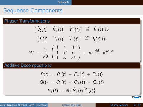
Sequence Components
Phasor Transformations[V0(t) V+(t) V−(t)
] def= V1(t)W[
I0(t) I+(t) I−(t)] def
= I1(t)W
W =1√3
1 1 11 α∗ α1 α α∗
, αdef= e j2π/3
Additive Decompositions
P(t) = P0(t) + P+(t) + P−(t)
Q(t) = Q0(t) + Q+(t) + Q−(t)
P+(t) = <
V+(t) IH+(t)
Alex Stankovic (Alvin H Howell Professor) Sparse Sampling Lagow Seminar 45 / 47
Sub-cycle
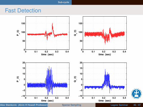
Fast Detection
0 0.1 0.2 0.3 0.40
50
100
150
time (sec)
P+
(t)
0 0.1 0.2 0.3 0.40
50
100
150
time (sec)
Q+
(t)
0 0.1 0.2 0.3 0.4−10
−5
0
5
10
15
20
time (sec)
P−
(t)
0 0.1 0.2 0.3 0.4−10
−5
0
5
10
15
20
time (sec)
Q−
(t)
Alex Stankovic (Alvin H Howell Professor) Sparse Sampling Lagow Seminar 46 / 47

ConclusionsThe reactive power story is an old (and formidable) problem,
Energy Processing Laboratory – p. 34/38

ConclusionsThe reactive power story is an old (and formidable) problem,
It has evolved as performance goals and compensationmeans have changed,
Energy Processing Laboratory – p. 34/38

ConclusionsThe reactive power story is an old (and formidable) problem,
It has evolved as performance goals and compensationmeans have changed,
Reading papers by old masters is a rewarding (andego-shrinking) experience,
Energy Processing Laboratory – p. 34/38

ConclusionsThe reactive power story is an old (and formidable) problem,
It has evolved as performance goals and compensationmeans have changed,
Reading papers by old masters is a rewarding (andego-shrinking) experience,
The electric energy engineering - Ars Longa, Vita Brevis.
Energy Processing Laboratory – p. 34/38

' $SELECTED REFERENCES
& %CURENT & NUCEER Centers, Northeastern University
• S. Fryze, “Active, Reactive and Apparent Power in Networks with Nonsinusoidal
Waveforms of Voltage and Current” (in German), Electrotechnische Zeitschrift, Vol.
53, No. 25, pp. 596-599, June 1932.
• C.I. Budeanu, “Puisance Reactives et Fictives,” Institut National Romain pour l’Etude
de l’Amenagement et de l’Utilisation des Sources de l’Energie, Vol. 2, Bucharest,
Romania, 1927.
• H. Lev-Ari and A.M. Stankovic, “A Decomposition of Apparent Power in Polyphase
Unbalanced Networks in Nonsinusoidal Operation,” IEEE Trans. on Power Systems,
Vol. 21, No. 1, pp. 438 - 440, Feb. 2006.
• H. Akagi, Y. Kanazawa and A. Nabae, “Instantaneous Reactive Power Compensators
comprising Switching Devices without Energy Storage Components,” IEEE Trans. on
Industrial Applications, Vol. 20, pp. 625-630, August 2004.
42