Electric Drives 1

9.11. FLUX OBSERVERS FOR DIRECT VECTOR CONTROL

WITH MOTION SENSORS

The motor stator or airgap flux space phasor amplitude ma and its

instantaneous position - er+a* - with respect to stator phase a axis have to be

computed on line, based on measured motor voltages, currents and, when available, rotor speed. The torque may be calculated from flux and current space phasors and thus once the flux is computed and stator currents measured, the torque problem is solved.

9.11.1. Open loop flux observers

Open loop flux observers are based on the voltage model or on the current model. Voltage model makes use of stator voltage equation in stator coordinates (from (9.32) with 1 = 0):

(9.95)s

ss

sss

s sirV

Electric Drives 2

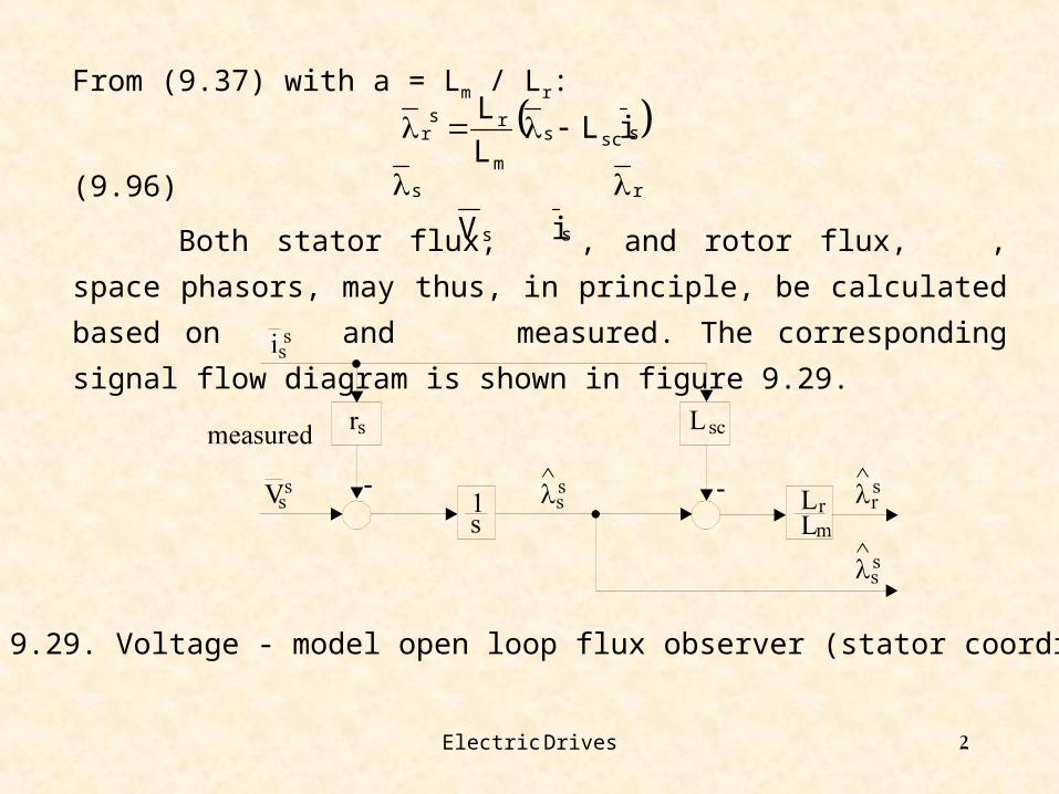
From (9.37) with a = Lm / Lr:

(9.96)

Both stator flux, , and rotor flux, , space phasors, may thus, in

principle, be calculated based on and measured. The corresponding signal

flow diagram is shown in figure 9.29.

sscs

m

rsr iL

L

L

Figure 9.29. Voltage - model open loop flux observer (stator coordinates)

s rsV si

Electric Drives 3

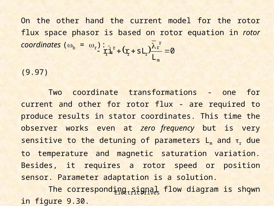
On the other hand the current model for the rotor flux space phasor is based

on rotor equation in rotor coordinates (b = r):

(9.97)

Two coordinate transformations - one for current and other for rotor

flux - are required to produce results in stator coordinates. This time the

observer works even at zero frequency but is very sensitive to the detuning of

parameters Lm and r due to temperature and magnetic saturation variation.

Besides, it requires a rotor speed or position sensor. Parameter adaptation is a

solution.

The corresponding signal flow diagram is shown in figure 9.30.

0L

sLrirm

rr

rrr

sr

Electric Drives 4

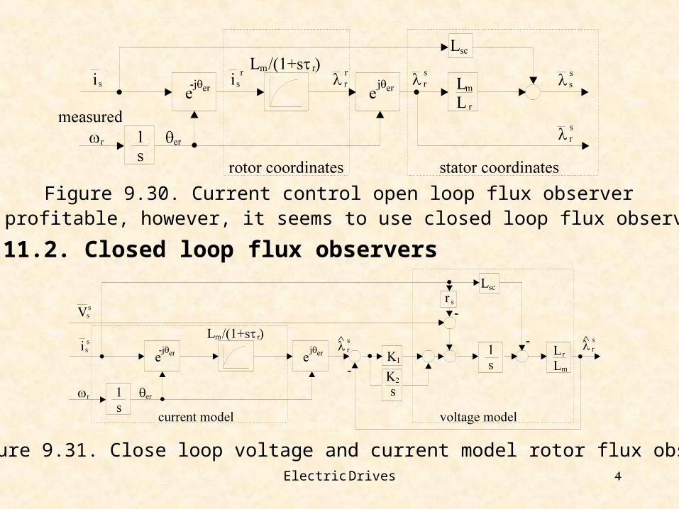
Figure 9.30. Current control open loop flux observerMore profitable, however, it seems to use closed loop flux observers.

9.11.2. Closed loop flux observers

Figure 9.31. Close loop voltage and current model rotor flux observer

Electric Drives 5

Many other flux observers have been proposed. Among them, the third flux

(voltage) harmonic estimator [21] and Gopinath observer [22], model

reference adaptive and Kalman filter observers.

They all require notable on line computation effort and knowledge of

induction motor parameters. Consequently they seem more appropiate when

used together with speed observers for sensorless induction motor drives as

shown in the corresponding paragraph, to follow after the next case study.

Electric Drives 6

9.12. INDIRECT VECTOR SYNCHRONOUS CURRENT CONTROL

WITH SPEED SENSOR - A CASE STUDY

The simulation results of a vector control system with induction motor based

on d.c. current control - are now given. The simulation of this drive is

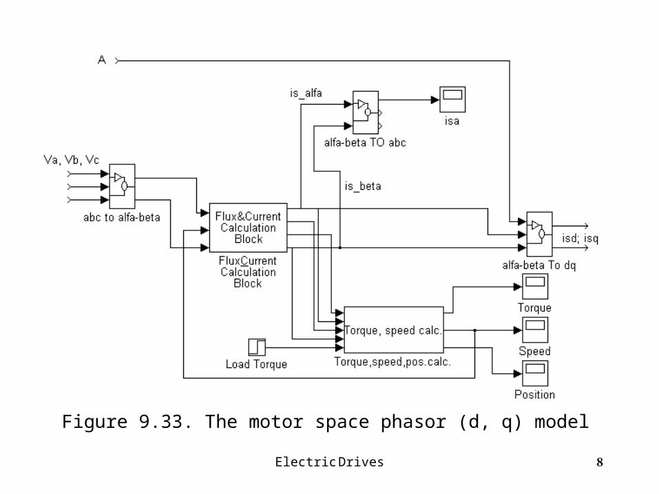
implemented in MATLAB - SIMULINK. The motor model was integrated in

two blocks, the first represents the current and flux calculation module in d -

q axis (figure 9.32), the second represents the torque, speed and position

computing module (figure 9.33).

The motor used for this simulation has the following parameters: Pn =

1100W, Vnf = 220V, 2p = 4, rs = 9.53, rr = 5.619, Lsc = 0.136H, Lr =

0.505H, Lm = 0.447H, J = 0.0026kgfm2.

Electric Drives 7

Figure 9.32. The indirect vector current control system

Electric Drives 8

Figure 9.33. The motor space phasor (d, q) model

Electric Drives 9

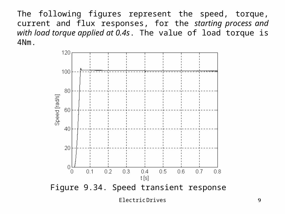
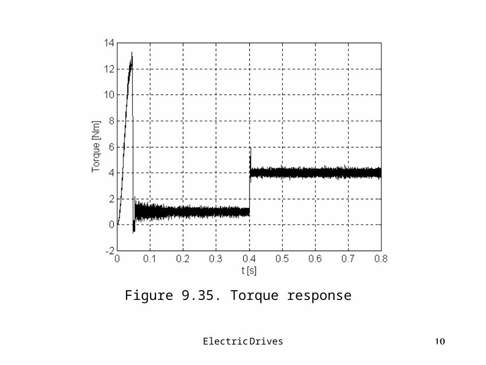
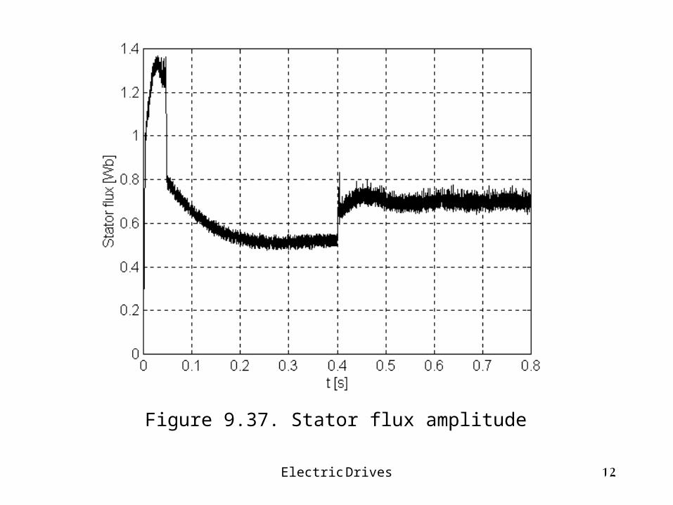
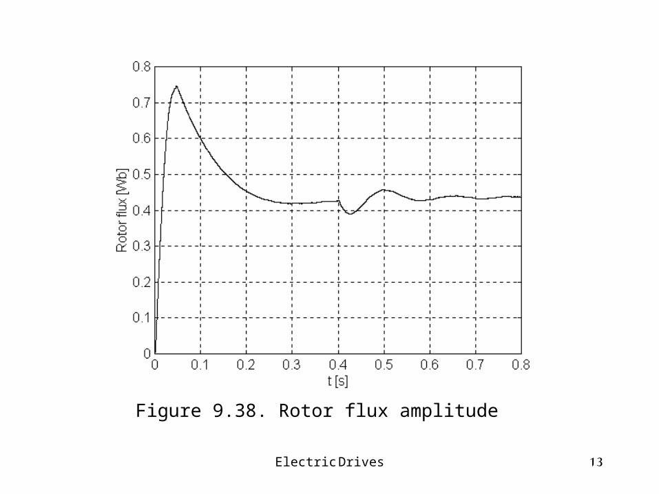
The following figures represent the speed, torque, current and flux responses, for the starting process and with load torque applied at 0.4s. The value of load torque is 4Nm.

Figure 9.34. Speed transient response

Electric Drives 10

Figure 9.35. Torque response

Electric Drives 11

Figure 9.36. Phase current waveform

Electric Drives 12

Figure 9.37. Stator flux amplitude

Electric Drives 13

Figure 9.38. Rotor flux amplitude

Electric Drives 14

9.13. FLUX AND SPEED OBSERVERS IN SENSORLESS DRIVES

Sensorless drives are becoming predominant when only up to 100 to 1 speed control range is required even in fast torque response applications (1-5ms for step rated torque response).

9.13.1. Performance criteria

To assess the performance of various flux and speed observers for sensorless drives the following performance criteria have become widely accepted:

steady state error; torque response quickness; low speed behaviour (speed range); sensitivity to noise and motor parameter detuning; complexity versus performance.

Electric Drives 15

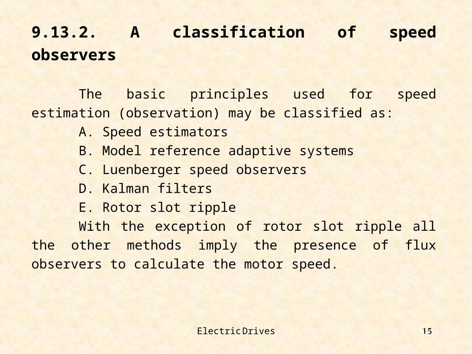
9.13.2. A classification of speed observers

The basic principles used for speed estimation (observation) may

be classified as:

A. Speed estimators

B. Model reference adaptive systems

C. Luenberger speed observers

D. Kalman filters

E. Rotor slot ripple

With the exception of rotor slot ripple all the other methods imply

the presence of flux observers to calculate the motor speed.

Electric Drives 16

9.13.3. Speed estimators

Speed estimators are in general based on the classical definition of

rotor speed :

(9.98)

where 1 is the rotor flux vector instantaneous speed and (S1) is the rotor

flux slip speed. 1 may be calculated in stator coordinates based on the

formula:

(9.99)

or (9.100)

r

^

^

11

^

r

^

S

qrdrs

rs

r1

^

j ;Argdt

d

2sr

sqr

sdr

sdr

sqr

1

^

Electric Drives 17

are to be determined from a flux observer (see figure 9.32,

for example). On the other hand the slip frequency (S1), (9.23), is:

(9.101)

Notice that is strongly dependent only on rotor resistance rr as

Lm / Lr is rather independent of magnetic saturation. Still rotor resistance is to

be corrected if good precision at low speed is required. This slip frequency

value is valid both for steady state and transients and thus is estimated

quickly to allow fast torque response.

Such speed estimators may work even at 20rpm although dynamic capacity of

torque disturbance rejection at low speeds is limited.

This seems to be a problem with most speed observers.

sqr

sdr

sdr

sqr ,,,

r

2r

mdsqrqsdr

rr2

r

mdsqrqsdr^

1

Lii

Lr/p23

Liip23

S

^

1S

r

^

Electric Drives 18

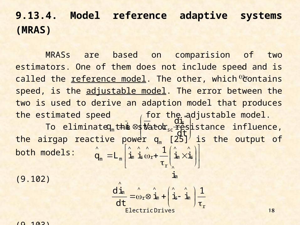
9.13.4. Model reference adaptive systems (MRAS)

MRASs are based on comparision of two estimators. One of them

does not include speed and is called the reference model. The other, which

contains speed, is the adjustable model. The error between the two is used to

derive an adaption model that produces the estimated speed for the

adjustable model.

To eliminate the stator resistance influence, the airgap reactive power

qm [25] is the output of both models:

(9.102)

(9.103)

The rotor flux magnetization current equation in stator coordinates

is ((9.15) with 1 = 0):

(9.104)

r

^

dt

idLViq

*s

scssm

s

^

m

^

r

r

^

s

^

m

^

mm

^

ii1

iiLq

m

^

i

r

m

^

s

^

m

^

r

^m

^

1iii

dt

id

Electric Drives 19

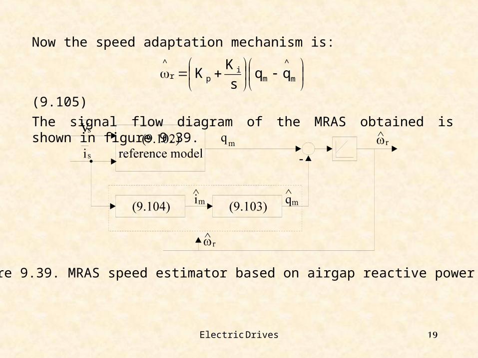
Now the speed adaptation mechanism is:

(9.105)

The signal flow diagram of the MRAS obtained is shown in figure 9.39.

m

^

mi

pr

^

qqs

KK

Figure 9.39. MRAS speed estimator based on airgap reactive power error

Electric Drives 20

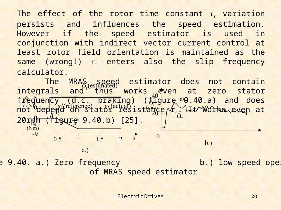
The effect of the rotor time constant r variation persists and influences the speed estimation. However if the speed estimator is used in conjunction with indirect vector current control at least rotor field orientation is maintained as the same (wrong!) r enters also the slip frequency calculator.

The MRAS speed estimator does not contain integrals and thus works even at zero stator frequency (d.c. braking) (figure 9.40.a) and does not depend on stator resistance rs. It works even at 20rpm (figure 9.40.b) [25].

Figure 9.40. a.) Zero frequency b.) low speed operation of MRAS speed estimator

Electric Drives 21

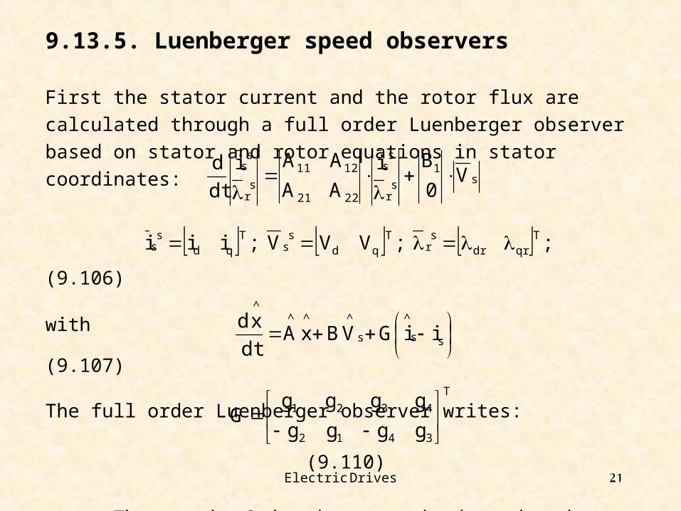
9.13.5. Luenberger speed observers

First the stator current and the rotor flux are calculated through a full order

Luenberger observer based on stator and rotor equations in stator coordinates:

(9.106)

with (9.107)

The full order Luenberger observer writes:

(9.110)

The matrix G is chosen such that the observer is stable.

(9.111)

s1

sr

ss

2221

1211

sr

ss

V0

Bi

AA

AAi

dt

d

; ;VVV ;iii Tqrdr

sr

Tqd

ss

Tqd

ss

ss

^

s

^^^^

iiGVBxAdt

xd

T

3412

4321

gggg

ggggG

Electric Drives 22

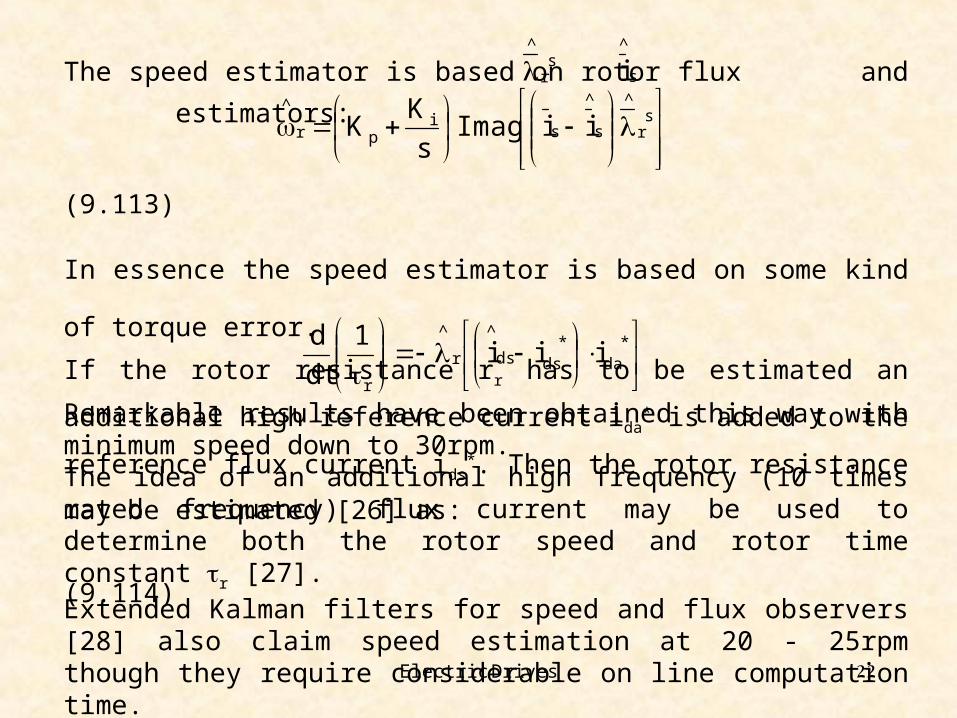
The speed estimator is based on rotor flux and estimators:

(9.113)

In essence the speed estimator is based on some kind of torque error.

If the rotor resistance rr has to be estimated an additional high reference

current ida* is added to the reference flux current ids

*. Then the rotor resistance

may be estimated [26] as:

(9.114)

sr

^

s

^

i

s

r

^

s

^

si

pr

^

iiagIms

KK

*da

*dsds

^

r

^

r

iii1

dt

d

Remarkable results have been obtained this way with minimum speed down to 30rpm.The idea of an additional high frequency (10 times rated frequency) flux current may be used to determine both the rotor speed and rotor time constant r [27].Extended Kalman filters for speed and flux observers [28] also claim speed estimation at 20 - 25rpm though they require considerable on line computation time.

Electric Drives 23

9.13.6. Rotor slots ripple speed estimators

The rotor slots ripple speed estimators are based on the fact that the

rotor slotting openings cause stator voltage and current harmonics s1,2 related

to rotor speed , the number of rotor slot Nr and synchronous speed :

(9.115)

Band pass filters centered on the rotor slot harmonics are used to

separate and thus calculate from (9.115). Various other methods have

been proposed to obtain and improve the transient performance. The

response tends to be rather slow and thus the method, though immune to

machine parameters, is mostly favorable for wide speed range but for low

dynamics (medium - high powers) applications [27].

For more details on sensorless control refer to [30].

r

^

1

^

1

^

r

^

r2,1s

^

N

2,1s

^

2,1s

^

2,1s

^

r

^

Electric Drives 24

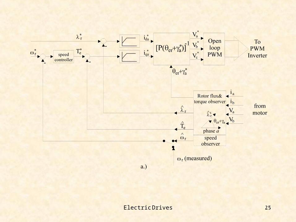
9.14. DIRECT TORQUE AND FLUX CONTROL

(DTFC)

DTFC is a commercial abbreviation for the so called direct self control

proposed initially [32 - 33] for induction motors fed from PWM voltage

source inverters and later generalized as torque vector control (TVC) in [4]

for all a.c. motor drives with voltage or current source inverters.

In fact, based on the stator flux vector amplitude and torque errors sign and

relative value and the position of the stator flux vector in one of the 6 (12)

sectors of a period, a certain voltage vector (or a combination of voltage

vectors) is directly applied to the inverter with a certain average timing.

To sense the stator flux space phasor and torque errors we need to estimate

the respective variables. So all types of flux (torque) estimators or speed

observers good for direct vector control are also good for DTFC. The basic

configurations for direct vector control and DTFC are shown on figure 9.41.

Electric Drives 25

Electric Drives 26

Figure 9.41. a.) Direct vector current control b.) DTFC control

As seen from figure 9.41 DTFC is a kind of direct vector d.c. (synchronous) current control.

Electric Drives 27

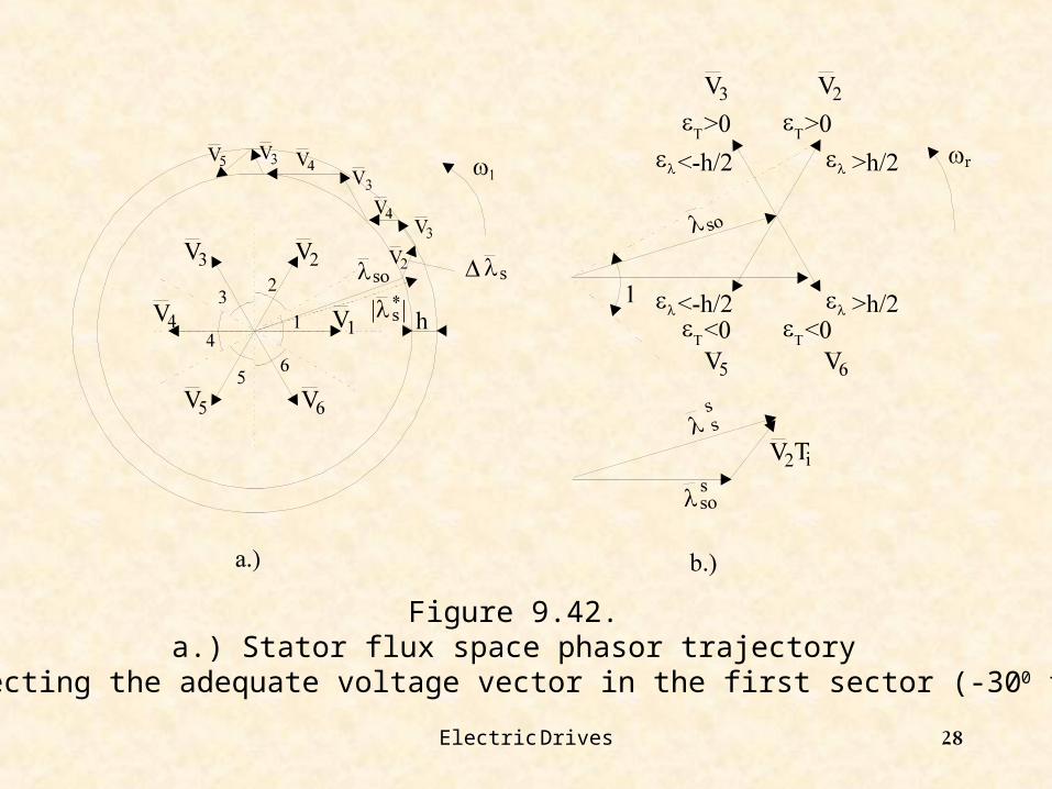
9.14.1. DTFC principle

Though figure 9.41 uncovers the principle of DTFC, finding how the

T.O.S. is generated is the way to a succesful operation.

Selection of the appropiate voltage vector in the inverter is based

on stator equation in stator coordinates:

(9.117)

By integration:

(9.118)

In essence the torque error T may be cancelled by stator flux

acceleration or deceleration. To reduce the flux errors, the flux trajectories will

be driven along appropriate voltage vectors (9.118) that increase or decrease

the flux amplitude.

iVs

sss

ss

ss

irVdt

d

is

T

0

sss

ss

s0s

ss

ss TiVdtirV

i

Electric Drives 28

Figure 9.42. a.) Stator flux space phasor trajectory

b.) Selecting the adequate voltage vector in the first sector (-300 to +300)

Electric Drives 29

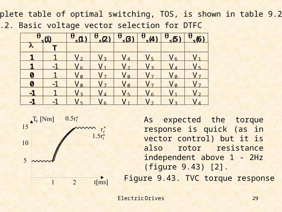
The complete table of optimal switching, TOS, is shown in table 9.2.

Table 9.2. Basic voltage vector selection for DTFC

s(i) s(1)

s(2) s(3)

s(4) s(5)

s(6) T1 1 V2 V3 V4 V5 V6 V1

1 -1 V6 V1 V2 V3 V4 V5

0 1 V0 V7 V0 V7 V0 V7

0 -1 V0 V7 V0 V7 V0 V7

-1 1 V3 V4 V5 V6 V1 V2

-1 -1 V5 V6 V1 V2 V3 V4

As expected the torque response is quick (as in vector control) but it is also rotor resistance independent above 1 - 2Hz (figure 9.43) [2].

Figure 9.43. TVC torque response

Electric Drives 30

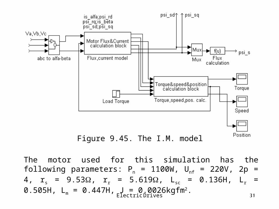
9.15. DTFC SENSORLESS: A CASE STUDYThe simulation results of a direct torque and flux control drive system for induction motors are presented. The example was implemented in MATLAB - SIMULINK. The motor model was integrated in two blocks, first represents the current and flux calculation module in d - q axis, the second represents the torque, speed and position computing module (figure 9.44).

Figure 9.44.The DTFC system

Electric Drives 31

Figure 9.45. The I.M. model

The motor used for this simulation has the following parameters: Pn = 1100W, Unf = 220V, 2p = 4, rs = 9.53, rr = 5.619, Lsc = 0.136H, Lr = 0.505H, Lm = 0.447H, J = 0.0026kgfm2.

Electric Drives 32

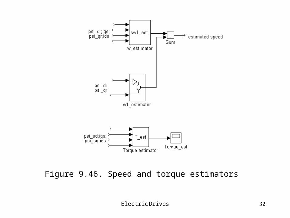
Figure 9.46. Speed and torque estimators

Electric Drives 33

Electric Drives 34

Figure 9.47. Speed transient response (measured and estimated)

Electric Drives 35

Figure 9.48. Phase current waveform (steady state)

Electric Drives 36

Electric Drives 37

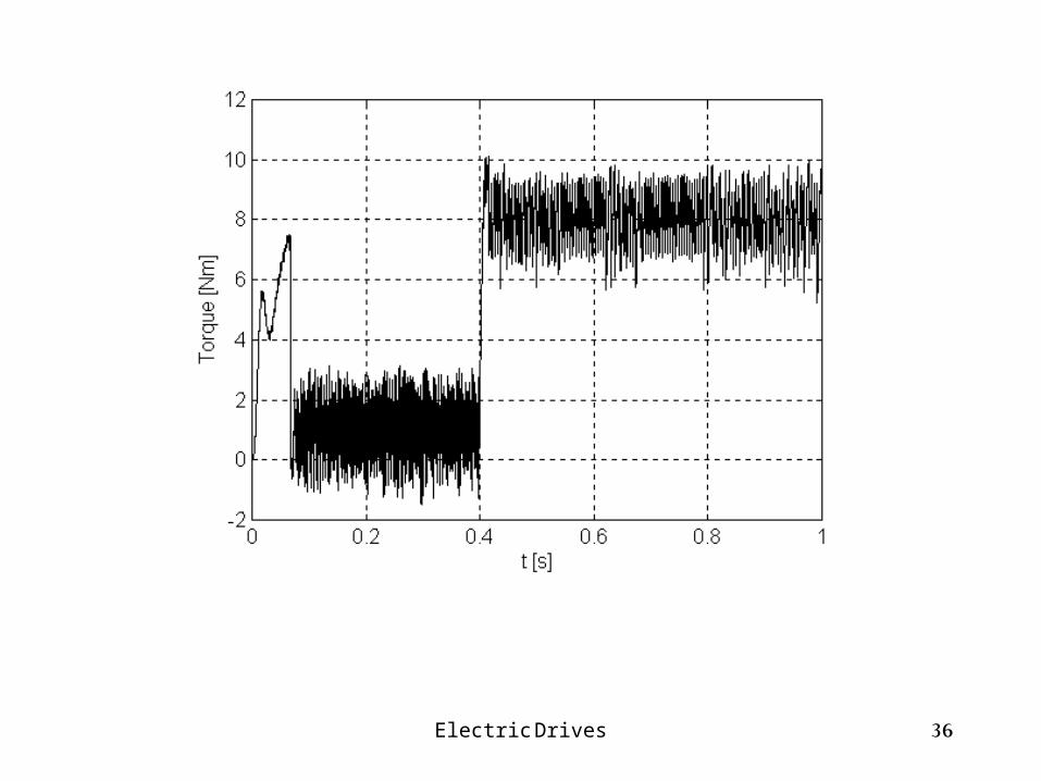
Figure 9.49. Torque response (measured and estimated)

Electric Drives 38

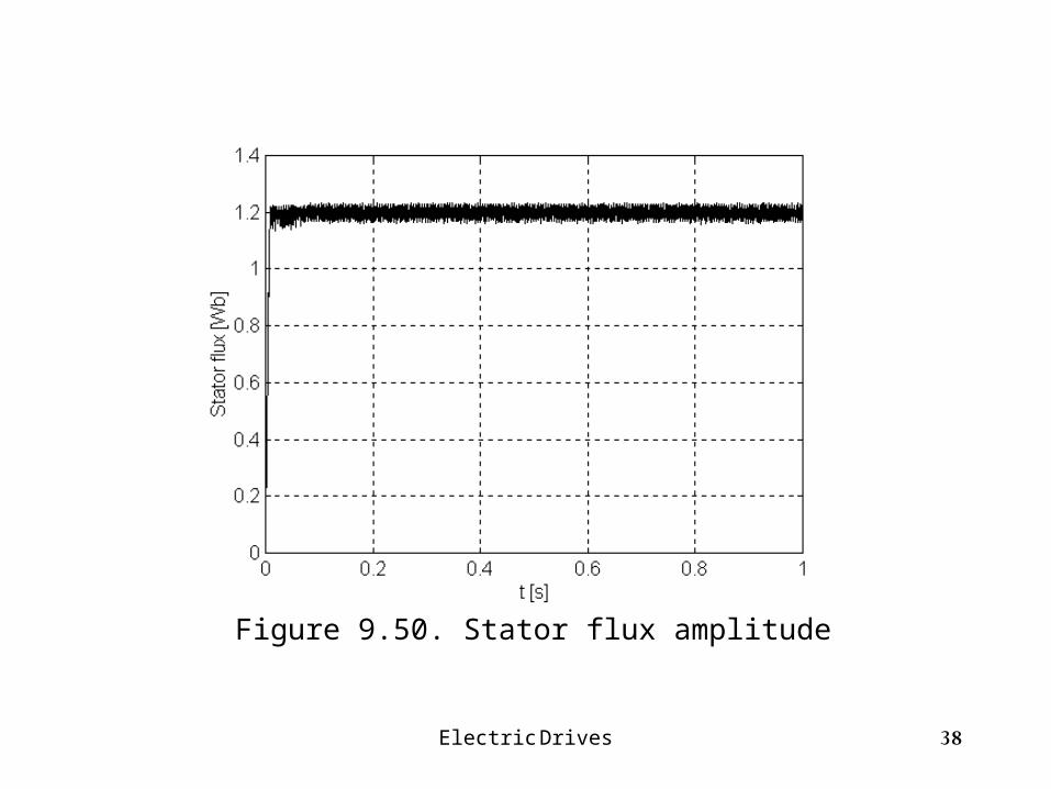
Figure 9.50. Stator flux amplitude

Electric Drives 39

Figure 9.51. Rotor flux amplitude