electoral systems and forms of...
TRANSCRIPT

ELECTORAL SYSTEMS AND FORMS
OF ABSTENTION
Orestis Troumpounis
Supervised by Enriqueta Aragones
Submitted to
Departament d’Economia i d’Historia Economica
at
Universitat Autonoma de Barcelona
in partial fulfillment of the requirements for the degree of
Doctor in Economics
May 2011
Acknowledgments
I am thankful to Enriqueta Aragon�es for giving me the chance to proudly be seen
by many political scientists as an economist, and by many economists as a political
scientist. I hope I have succeeded in absorbing part of her interdisciplinarity,
perfectionism, critical approach and spirit. Having the chance to learn from her
about Economics, Politics, Catalunya and life has been the biggest reward during
this trip. I am thoroughly obliged to her for all her e�orts and support.
I would like to thank Helios Herrera, Humberto Llavador, and Santiago Sanchez
for kindly accepting to be members of the committee, Andrea Mattozzi for his con-
structive suggestions and discussions during these years, and Caterina Calsamiglia
for her useful comments and our good collaboration.
A special thanks to Carmen Bevia for taking time to read into detail much of
my work, and always provide me with honest, direct and constructive recommen-
dations. I am grateful to Clara Ponsati, both for her comments, and for helping
me during these years with my stay in UAB and Barcelona.
I bene�ted from the discussions with Jordi Masso, Hannes Mueller, and other
IDEA faculty members. Thanks to Jon Eguia, Howard Rosenthal, and Michael
Laver for their hospitality and lessons during my stay at NYU.
Here come my fellows, Evi, E�, Dimitri, Philippe, ��0��� ���� ��� �βρ�����!.
Thanks to Riste for transmitting serenity and keeping the spirits fun, to Sabine
for making the PhD seem one day closer, or one month further depending on her
day, to Lorenzo for being my travel buddy, and all IDEA colleagues for making
these years more comfortable.
I am indebted to my parents and sister for sustaining and motivating me
constantly, although I still deny to explain them what is a PhD in economics, how
and why I am about to become a \real" economist.
Finally, thanks to Faustine for making my grey days shine with her smile and
love, for supporting me, and keeping me happy during these years.
ii

CONTENTS
Contents
1 General Introduction 1
2 Engineering Electoral Systems to Increase Turnout 4
2.1 Introduction . . . . . . . . . . . . . . . . . . . . . . . . . . . . . . 4
2.2 Related Literature . . . . . . . . . . . . . . . . . . . . . . . . . . 8
2.3 The Model . . . . . . . . . . . . . . . . . . . . . . . . . . . . . . . 10
2.4 Varying Size Parliament . . . . . . . . . . . . . . . . . . . . . . . 11
2.4.1 Comparing VSP and FSP . . . . . . . . . . . . . . . . . . 13
2.5 Introducing a participation quorum q > 0 . . . . . . . . . . . . . . 15
2.5.1 Symmetric Equilibria . . . . . . . . . . . . . . . . . . . . . 16
2.5.2 Characterizing All Possible Equilibria . . . . . . . . . . . . 20
2.6 Discussion of the Voters' Decision . . . . . . . . . . . . . . . . . . 25
2.7 Conclusion . . . . . . . . . . . . . . . . . . . . . . . . . . . . . . . 26
2.8 Appendix . . . . . . . . . . . . . . . . . . . . . . . . . . . . . . . 29
3 Participation Quorums in Costly Meetings 47
3.1 Introduction . . . . . . . . . . . . . . . . . . . . . . . . . . . . . . 47
3.2 The Model . . . . . . . . . . . . . . . . . . . . . . . . . . . . . . . 50
3.2.1 The Setup . . . . . . . . . . . . . . . . . . . . . . . . . . . 50
3.2.2 The Exit Process . . . . . . . . . . . . . . . . . . . . . . . 51
3.2.3 The Quorum Game . . . . . . . . . . . . . . . . . . . . . . 55
3.3 Results . . . . . . . . . . . . . . . . . . . . . . . . . . . . . . . . . 56
3.3.1 The Benchmark: The No-Quorum Game . . . . . . . . . . 56
3.3.2 The Quorum Game . . . . . . . . . . . . . . . . . . . . . . 60
3.4 Conclusion . . . . . . . . . . . . . . . . . . . . . . . . . . . . . . . 67
iii
CONTENTS
3.5 Appendix . . . . . . . . . . . . . . . . . . . . . . . . . . . . . . . 69
4 Institutions, Society or Protest? Understanding Blank and Null
Voting 79
4.1 Introduction . . . . . . . . . . . . . . . . . . . . . . . . . . . . . . 79
4.2 Contribution to the Literature . . . . . . . . . . . . . . . . . . . . 84
4.3 Why Voters Cast a Blank or a Null Vote? . . . . . . . . . . . . . 85
4.4 Empirical Evidence . . . . . . . . . . . . . . . . . . . . . . . . . . 89
4.4.1 Data and The Model . . . . . . . . . . . . . . . . . . . . . 89
4.4.2 Empirical Results . . . . . . . . . . . . . . . . . . . . . . . 94
4.5 Conclusion . . . . . . . . . . . . . . . . . . . . . . . . . . . . . . . 98
4.6 Appendix . . . . . . . . . . . . . . . . . . . . . . . . . . . . . . . 100
iv
Chapter 1
General Introduction
The present thesis lies at the intersection of economics and political science.
Using methods, well developed in economics, I try to understand how electoral
institutions shape individuals' behavior in di�erent political contexts. The three
chapters are closely related, and focus from three di�erent perspectives on the
decision of voters to abstain or to participate in an election.
Chapter 2 has a normative avor, and is motivated by my personal frustration
towards the dangerous combination of apathetic citizens and mediocre politicians
prevailing in contemporary politics. Focusing on the interplay between low quality
parties and citizens' apathy, I try to break the vicious cycle that links the two,
by proposing two electoral rules that increase turnout in PR elections, and at the
same time give incentives to parties to be of better quality.
First, I propose an electoral rule where the number of candidates elected de-
pends on the level of participation. Second, I propose the introduction of a par-
ticipation quorum that has to be met in order for the election to be valid. The
common feature and innovation of these rules is that turnout a�ects the electoral
outcome, and as a consequence these rules incentivize parties to care about the
level of turnout. I show that both rules, while they increase turnout they imply
lower pro�ts for parties. My results explain why parties target to increase turnout
through a certain type of measures that do not necessary improve the quality of
the vote. Moreover, I also explain the evolution of the use of the participation
quorum in certain countries.
1
General Introduction
In reality, a participation quorum is not often present neither in parliamentary
nor in presidential elections. On the contrary, in many small scale meetings, for
example, meetings of shareholders, members of societies, and clubs, the number
of attendees must exceed an exogenously given participation requirement in order
for a decision to be taken. Otherwise, the meeting can not take place, and it has
to be postponed for the future.
Chapter 3 is coauthored with Sabine Flamand, and tries to understand the
e�ect of such a participation requirement on individuals' behavior and the decision
outcome. To this end, we model a setup of repeated meetings, where a small group
of individuals has to take a decision. We show that the decision is delayed when
the quorum requirement is high and members are not harmed by postponing
the decision. Surprisingly, the presence of the quorum may decrease the number
of attendees taking the decision, while we show that in order to avoid policy
distortions, the required number of participants must be even.
Although presented as the last chapter of this thesis, Chapter 4 is the one I
completed �rst. While browsing the political science literature in order to motivate
a previous version of Chapter 2, I realized that several questions that seemed
natural to me, had not been answered. Apart from abstaining, voters that are
not willing to support any of the candidates in most parliamentary elections, are
given the choice to participate in the election and cast a blank or a null vote. A
blank vote is a disapproval vote of all competing candidates, while a null vote
is a vote cast erroneously or deliberately in a way not conforming with the legal
voting procedure.
Political scientists were treating blank and null votes in an identical way. My
attempt in this chapter is to study these two protest actions on a separate basis, in
order to understand, why in some elections blank votes are many more than null
votes and vice versa. After constructing a database considering the percentages
of blank and null votes separately, I show that the amount of blank and null
votes cast in an election are not a�ected by the same factors. Null votes convey
dissatisfaction towards the electoral and democratic institutions, while blank votes
convey dissatisfaction towards the parties. More important, my results go against
one of the prevailing criticisms of compulsory voting. The latter has no signi�cant
e�ect on the amount of uninformative votes since it has no signi�cant e�ect on the
2

amount of null votes. On the contrary, it increases only the amount of blank votes,
which by de�nition disclose information, and in particular voters' disapproval of
all competing parties.
Although abstention is one of the most studied issues both by political scien-
tists and economists, I hope that the current thesis extends our knowledge, by
giving insight into some of abstention's unexplored but widely observed aspects.
Moreover, I hope that this thesis not only succeeds in analyzing from a positive
perspective di�erent forms of abstention as political actions, but also by taking a
normative stance, and in particular by designing a set of modi�cations in existing
electoral systems. If one believes that the quality of democracy is determined by
the performance of its principal actors, then by giving incentives to parties to be
of better quality, and at the same time involving more citizens in the electoral
procedure, the suggestions of this thesis can eventually be considered as a way to
establish a better functioning of contemporaneous democracy.
3
Engineering Electoral Systems to Increase Turnout
Chapter 2
Engineering Electoral Systems toIncrease Turnout
2.1 Introduction
\Voice and exit are often alternative ways of exerting in uence, but
with regard to voting the exit option spells no in uence; only voice
can have an e�ect", Lijphart (1997)
Lijphart refers to abstention as the exit option of voters in elections. Indeed
in parliamentary elections voters abstaining do not a�ect the composition of the
parliament. In this paper we introduce two electoral rules under which the exit
option (i.e. abstention) in uences the outcome of the election. Both electoral
rules can be introduced as a solution to low turnout levels.
A well established empirical fact is that turnout is decreasing in most elections
during the last decades and more speci�cally since the mid-eighties (see Figure
1 in the appendix). A natural question that may arise is why it is of interest
going against this trend. In general, high levels of participation in democratic
elections are desirable in order to guarantee the legitimacy of the election, of
the elected government, of the representative institutions and of the democratic
political system as a whole. This can be re ected in president Barroso's speech
in 2009 right before the election for the EU parliament: “A low turnout in the
elections for the European Parliament next week would undermine the credibility
of the European Union in general and of the parliament in particular”. In this
4

2.1 Introduction
particular election the turnout rate was the lowest in the history of the EU (see
Figure 2 in the appendix) and as a result the vice-president of the EU commission
claimed that “...low turnout was a “bad result”... there is need for a radical shake-
up of how future European election campaigns are conducted by EU states, to try
to boost voter turnout”.
The most extreme among all alternatives in order to increase turnout is the
introduction of compulsory voting1. As expected, it is shown both empirically
(Jackman, 1987; Blais and Dobrzynska, 1998; Franklin, 1999, 2004) and experi-
mentally (Hirczy, 1994) that compulsory voting is associated with higher levels of
turnout. In his presidential speech of the American Political Science Association,
Lijphart endorsed compulsory voting and claimed that “it is the only institutional
mechanism that can assure high turnout virtually by itself”.
While the e�ectiveness of compulsory voting in increasing turnout can not be
challenged, there exist several arguments against it. The typical normative argu-
ment is that in the e�ort to enhance democracy the tool is highly \undemocratic"
since it restricts citizens' right not to vote. Furthermore, although compulsory
voting increases turnout, it does not improve on the quality of the vote since it
increases the numbers of uninformed voters who are forced to participate.
As a solution to low turnout under a PR system we suggest two electoral rules
that may a�ect the e�ort exerted by parties: a varying size parliament and the
introduction of a participation quorum.
In the case of a varying size parliament (VSP) the number of candidates elected
depends on the level of participation2. It is actually determined after the election
takes place and abstention is translated into empty seats in the parliament. The
di�erence between a �xed size parliament (FSP) and a VSP is the seat allocation
1As an alternative to compulsory voting, rather than punishing voters for not voting one couldreward them for voting. This form of incentives could be either a flat-rate payment to everyvoter or the right to participate in a lottery that assigns a prize to a lucky participant. While aflat rate payment has not been implemented, the case of a lottery has been practiced in the 2005parliamentary election in Bulgaria and in 1995 in municipality elections in Norway. Gerardiet al. (2009) compare theoretically and in laboratory experiments the case of compulsory votingversus incentives through a lottery. While both increase turnout, lotteries are more effective interms of information aggregation.
2The idea of a VSP is similar to a seat allocation method based on a fixed quota. Forexample, in the elections of 1919 in Weimar Republic, parties had to obtain 60.000 votes for oneseat in the parliament(Colomer, 2004).
5

Engineering Electoral Systems to Increase Turnout
after the election takes place. In the case of a FSP the number of candidates
elected is �xed and does not depend on turnout while under a VSP the number
of candidates elected depends on participation.
Alternatively, rather than varying the number of candidates elected, one could
think of varying the length of the term that elected candidates stay in o�ce. In
this case the length of the term is endogenously determined and depends on the
level of participation. If for example the normal term is four years and only half
of the population participates then the term will be reduced to two years.
A last important interpretation of the VSP with direct policy implications
is associated with parties' public funding. A VSP can be thought as a funding
system where parties are funded per vote and hence the total transfers to parties
depends on the level of participation. On the contrary, the FSP can be interpreted
as a funding system where the total amount of transfers to parties is �xed and
the funds are allocated to each party based on each party's representation in the
parliament.
The second electoral rule we analyze in order to increase turnout, is the intro-
duction of a participation quorum. If the participation quorum is not met then
candidates do not acquire any seats in the parliament thus they obtain zero ben-
e�t. In such a case a new election takes place. We assume that there are no �xed
costs for organizing an election.
The common feature of both suggested electoral rules (i.e. a switch to a VSP
and the introduction of a participation quorum) is that the level of abstention
a�ects the electoral outcome and the composition of the parliament. The advan-
tage of the two suggested alternatives over compulsory voting is that they do not
\oblige" voters to participate3. They rather incentivize parties to care about the
level of participation.
In order to study the e�ect of the two above alternatives we adapt a group-
based model of turnout (Snyder, 1989; Shachar and Nalebu�, 1999; Herrera and
Mattozzi, 2009). In this type of models parties exert some costly e�ort that is
bene�cial for voters. The e�ort that parties exert may be interpreted in several
ways. The �rst interpretation is that e�ort is directly related to the mobilization
3Under compulsory voting a voter may still abstain. We say that voters are obliged to votein order to avoid a possible sanction.
6
2.1 Introduction
actions taken by parties. Gerber and Green (2000) through a random experiment
show evidence of the relationship between mobilization and the decision to vote.
Citizens that are informed by parties on a personal basis, vote with higher prob-
ability. In general, they conclude that time consuming and costly mobilization
e�ort such as canvassing has a higher e�ect turnout than less costly e�ort such
as telephone calls and electronic mails. Similarly, e�ort can be interpreted as the
social pressure put by parties in order to mobilize voters. As Shachar and Nalebu�
(1999) claim, through social pressure parties can mobilize voters by increasing the
cost of non-voting. Indeed, Gerber et al. (2008) o�er experimental evidence and
show that individuals receiving social pressure participate in the election with
higher probability.
Another interpretation of e�ort is the quality of each party as in Carrillo and
Castanheira (2008). Hiring experts or the opportunity cost of parties of not being
corrupt (Polo, 1998) are examples of why parties' quality is costly. When parties
are of better quality, voters obtain a higher bene�t and are willing to pay the cost
of participating. No matter which interpretation we give to e�ort, the important
element for our analysis is that e�ort is costly for parties while it is desirable for
voters.
Each voter has a personal cost of voting that is private information. We assume
that each individual may vote for his favorite party or abstain, therefore there are
no swing voters. Voters are expressive and support their preferred party if the
e�ort exerted by the party is high enough to compensate the cost of participating.
In our model there are two exogenously given parties and the society is divided
into two pools of potential voters for each party. One of the parties may have a
larger support than the other and thus may enjoy an advantage. Parties' pro�ts
depend on the the absolute number of seats won. The cost that parties have to
bare depends on the e�ort they exert in order to convince their supporters to
participate.
We begin our analysis with the case FSP which is our benchmark case. We
show that despite a possible advantage of one party in terms of its initial support,
there exists a unique symmetric equilibrium. On the contrary, under a VSP the
equilibrium e�ort level is asymmetric in case of di�erent initial support for each
party. The reason why under a FSP we obtain only symmetric e�ort level is that
7
Engineering Electoral Systems to Increase Turnout
under a FSP the game is constant sum where parties share the same amount of
seats in the parliament independently of the turnout level, while under a VSP this
is not the case since the number of seats available is increasing in turnout.
More important, when comparing turnout under a FSP and a VSP, we show
that a VSP implies higher turnout only when parties obtain high bene�ts for being
represented in parliament. Moreover, when the introduction of a VSP implies
higher turnout then parties obtain lower pro�ts.
With respect to the second electoral rule, we show that there exists a range
of participation quorums that boost turnout. If the exogenously given quorum
falls in that range then in equilibrium it is always binding. We show that there
exists a unique symmetric equilibrium, where both parties exert the same amount
of e�ort. If so, parties obtain lower pro�ts when competing in an election with
a participation quorum requirement than when competing in an election with no
quorum requirement. Despite the symmetric setup in terms of support, we show
that there exist multiple asymmetric equilibria, where one party exerts higher
e�ort than the other. Even in this case, the total e�ort exerted by parties is such
that the participation quorum in equilibrium is binding.
The paper is organized as follows. In section two we compare our work to the
existing literature and discuss our contribution to it. In section three we present
the model. In section four we characterize and compare equilibria for both the
FSP and the VSP. In section �ve we introduce a participation quorum and again
we characterize and compare equilibria under both a FSP and a VSP. In section
six we o�er a spatial interpretation of the voters' decision rule and in section seven
we conclude.
2.2 Related Literature
The characterization of the optimal level of turnout and the e�ects of compul-
sory voting had received very little attention by economists till recently. The �rst
contribution focusing on compulsory voting is by B•orgers (2004). He analyzes
a costly voting model and he shows that in a symmetric setup, under majority
voting, voluntary participation Pareto dominates compulsory voting. This is be-
8
2.2 Related Literature
cause voting can be thought of as a negative externality problem. Any additional
vote makes it less likely that any other individual's vote is pivotal. Hence, in
equilibrium participation in elections is already too high and compulsory voting
moves turnout the wrong direction.
On the contrary, Krasa and Polborn (2009); Ghosal and Lockwood (2009) show
that increasing turnout may be e�cient. Under di�erent assumptions they show
that one's vote may create a positive externality on top of the negative \pivot" ex-
ternality identi�ed by B•orgers (2004). When the positive externality compensates
the negative externality then in equilibrium turnout is low and hence increasing
turnout would be bene�cial. This is the case when there exists a su�ciently large
asymmetry in terms of the support of each candidate (Krasa and Polborn, 2009)
or when voting takes place according to signals since one's vote may improve the
quality of the decision for all voters (Ghosal and Lockwood, 2009).
Our group-turnout model (Snyder, 1989; Shachar and Nalebu�, 1999; Herrera
and Mattozzi, 2009) di�ers from the above since our voters' decision to participate
depends on a bene�t associated with parties' e�ort rather than the probability
of being pivotal. Regarding group-turnout models and although our research
question is quite di�erent from the one of Shachar and Nalebu� (1999), the authors
o�er interesting interpretations of why e�ort exerted by some voters (the so called
leaders) may mobilize the rest of the voters (the so called followers). For example,
e�ort exerted by leaders may decrease the direct cost of voting and the cost of
information acquisition. We provide a spatial interpretation of the voter's decision
and we motivate e�ort as the quality of the party.
A similar group-based model is used by Herrera and Mattozzi (2009) to study
the e�ect of a participation quorum in referenda. In contrast to our setup, they
show that the participation quorum in case of referenda may result into lower
participation levels. This is the case when the party supporting the status quo has
incentives to stay passive rather than mobilizing it's supporters to vote against the
change. By not mobilizing it's voters it \wins" the referendum by not satisfying
the participation quorum. This is not the case in our model, since both parties
have incentives to mobilize the supporters in order to avoid a new election.
9

Engineering Electoral Systems to Increase Turnout
2.3 The Model
There are two exogenously given parties j = L;R. The society is divided into
two pools of potential supporters of each party. Without loss of generality, we
assume that fraction � 2 [0:5; 1) supports party L, with the remaining (1 � �)
denoting the support of party R. Each voter has a personal cost of voting c 2 [0; 1]
that is private information. We assume that parties' beliefs on the value of c are
represented by an i.i.d. uniform distribution on [0; 1].
Parties decide simultaneously the amount of e�ort to exert in order to per-
suade their supporters to vote for them. We assume that voters receive a bene�t
from voting their preferred party that is strictly concave in parties e�orts. More
speci�cally, if party j exerts e�ort �j, the bene�t of voters supporting party j is
captured by the function �(�j). Function �(�j) : R+ ! [0; 1] , is continuous for
�j > 0, strictly increasing, strictly concave and takes value �(0) = 0. The voting
rule followed by the individuals is as follows: For a given level of e�ort made by
party j, a voter that supports party j and has a voting cost equal to c votes for
party j if and only if �(�j) > c.
From the parties' point of view and the uniformly distributed cost of voting
the probability that an individual participates is Pr(�(�j) > c) = �(�j), which
implies that the expected vote share for each party is equal to its initial support
multiplied by the probability that an individual participates (i.e. vL = ��(�L)
and vR = (1� �)�(�R)).
Abstention is given by: vA = 1� vL � vR = 1� ��(�L)� (1� �)�(�R). Notice
that abstention is always decreasing in both �L and �R.
Parties pro�ts are equal to the bene�ts parties obtain for holding seats in
parliament minus the cost parties have to pay in order to exert some e�ort. Parties
pro�t function is de�ned as:
�j = bsj � �j
where b > 0 is the payo� to a party if it were to obtain all the seats in the
parliament and sj is the percentage of seats the party obtains4. For simplicity, we
4The assumption of seat maximizing parties is necessary in order to compare a VSP anda FSP system. The difference between the FSP and the VSP results from the seat allocation
10

2.4 Varying Size Parliament
assume that for both parties the marginal cost of e�ort is equal to one5.
2.4 Varying Size Parliament
We begin our analysis with our benchmark case, the FSP system. Party L
exerting e�ort �L obtains vote share vL = ��(�L) and after the seat allocation its'
seat share is given by sFL = vLvL+vR
= ��(�L)��(�L)+(1��)�(�R)
which is the vote share of
party L divided by the turnout level. In the same way party R obtains seat share
sFR = (1��)�(�R)��(�L)+(1��)�(�R)
which is the vote share of party R divided by the turnout
level.
Proposition 1. Under a FSP there exists a unique equilibrium �FL(b; �) = �FR(b; �) =
�F (b; �), where �F (b; �) is the unique solution of �0(�F )�(�F )
= 1b�(1��)
All Proofs can be found in the Appendix
According to the above proposition in case of a FSP and even in cases that
parties have di�erent support (i.e. in case that � 6= 12), both parties exert the
same level of e�ort �F (b; �). The equilibrium e�ort level depends on both the
bene�t parties obtain and on the (a)symmetry of the society.
The symmetric equilibrium in terms of e�ort level despite a possible asymmetry
in terms of each party's initial support, is a consequence of the fact that parties
compete in a constant-sum game. The constant-sum game implies that what one
party wins in terms of seat share by increasing its e�ort level is exactly what the
other party looses in terms of seat share. Given that by assumption parties have
the same marginal cost (in this case equal to one) and because of the constant-sum
nature of the game, parties stop investing in e�ort at the same level (i.e. �F (b; �)).
and the absolute number of seats that each party obtains after the election. In order for thecomparison between the two systems to make sense it has to be the case that parties care forthe absolute number of seats rather than only the probability of winning. If parties care onlyfor the majority the solution of the maximization problem would be the same under both a FSPand a VSP.
5This assumption can be relaxed and does not affect our analysis. In general if both partieshave the same support and one party were able to increase its effort at a lower cost than theother party then it would exert higher effort than the other party.
11

Engineering Electoral Systems to Increase Turnout
Proposition 2. Under a FSP, �F (b; �) is strictly increasing in b and strictly
decreasing in �.
E�ort level exerted by each party is higher in more symmetric societies. Given
that in our setup, more symmetric societies implies a closer election, our result
is in line with a well established empirical fact, turnout is higher in closer races.
Moreover, e�ort level and turnout are increasing in the bene�t parties obtain.
When the bene�t is high, parties have more incentives to mobilize their supporters
to participate. As a result of this higher e�ort, turnout is higher.
Claim 1. Under a FSP in equilibrium �FL (b; �) > �FR(b; �), with the equality
holding for � = 0:5
When one of the parties has an advantage in terms of support then it makes
higher pro�ts. This is because in equilibrium both parties exert the same e�ort,
which implies that while they bare the same cost, the same amount of e�ort
translates into more votes and hence seats in the parliament for the advantaged
party.
Now we move to the case of the varying size parliament (VSP). The di�erence
with the FSP is the seat allocation. In case of the VSP we have sVL = vL = ��(�L)
and sVR = vR = (1 � �)�(�R). Since the vote share of each party is translated in
the seat share of each party in the parliament there is no reason to divide by the
participation level as in the case of a FSP. In case of a VSP the seat share of each
party does not depend on the vote share of the other party.
Proposition 3. Under a VSP there exists a unique equilibrium (�VL (b; �); �VR(b; �)),
where �VL (b; �) is the unique solution of �0(�VL ) = 1b�
and �VR(b; �) is the unique so-
lution of �0(�VR) = 1b(1��)
.
In the case of a VSP parties do not exert the same level of e�ort when they
have di�erent support. This is di�erent than in the case of a FSP and this is a
consequence of the fact that now the game is not a constant-sum one any longer
since under a VSP the number of seats in the parliament is not �xed. Although
both parties have the same marginal cost, the marginal bene�t of their e�ort level
is di�erent (higher for the case of the advantaged party) and hence the solution
of their maximization problem is di�erent.
12
2.4 Varying Size Parliament
Proposition 4. Under a VSP �VL (b; �) > �VR(b; �) with the equality holding for
� = 0:5. Both �VL (b; �) and �VR(b; �) are strictly increasing in b. �VL (b; �) is strictly
increasing in �, while �VR(b; �) is strictly decreasing in �.
In contrast to the FSP, the advantaged party always exerts higher e�ort when
� 6= 0:5. As in the case of a FSP both parties exert higher e�ort when they
obtain higher bene�t for being in parliament. This is because they have more
incentives to mobilize their supporters given the higher bene�t. When � increases
then party's L support increases while party's R support (i.e. 1 � �) decreases.
Hence, when � increases then party L increases its e�ort and party R decrease's
its e�ort. This implies that when the society is more asymmetric, the di�erence
between the e�ort level exerted by the two parties is larger.
Claim 2. Under VSP in equilibrium �VL > �VR with the equality holding for � =
0:5.
If one party has an advantage then it makes higher pro�ts. This time the
intuition is slightly di�erent than in the case of a FSP. In contrast to a FSP
the advantaged party exerts higher e�ort than its opponent. This implies that it
bares higher costs than the disadvantaged party. At the same time the advantaged
party obtains more seats in the parliament than the disadvantaged both because
of its higher e�ort and its higher support. Eventually, despite the higher cost that
the advantaged party has to pay, because of the concavity of the voters' bene�t
function the advantaged party's higher e�ort implies much higher seat share than
the disadvantaged party and hence higher pro�ts for the advantaged party.
2.4.1 Comparing VSP and FSP
Having analyzed separately the two electoral systems and having proved the
uniqueness of equilibria in both cases, the following proposition compares the two
systems. The results of this proposition are illustrated in �gure 1.
Proposition 5. For a given �, �VL (b) > �F (b) if and only if b > b. Moreover
�VR(b) > �F (b) if and only if b > b.
13

Engineering Electoral Systems to Increase Turnout
Figure 1
0
0
b
Effor
t
bb --
εεε F
V VL R
From the above proposition we conclude that which electoral system implies
higher e�ort depends on the level of b. If b > b then by introducing a VSP e�ort
increases for both parties. In our model a VSP would imply higher e�ort by both
parties if turnout under a FSP is larger than �. In the other extreme case, if b < b
then a VSP implies lower e�ort by both parties. This is the case when turnout is
lower than 1 � �. If b < b < b (or turnout is between 1 � � and �), then a VSP
implies higher e�ort by the advantaged party and lower e�ort by the one with
lower support.
Regarding turnout, if b > b both �VL and �VR are higher than �F and this implies
that turnout under a VSP is higher than turnout under a FSP. On the other
hand, if b < b both �VL and �VR are smaller than �F . This implies that if b < b
then the introduction of a VSP would imply even lower turnout than in the case
of a FSP. If b < b < b then �VL > �F > �VR. The combination of higher e�ort
by the advantaged party and lower e�ort by the disadvantaged one under a VSP
compared to the case of a FSP does not allow us to infer the total e�ect of the
introduction of a VSP on turnout. Concluding, a VSP can always be used as a
tool to increase turnout if under a FSP turnout is higher than �. In general, a
VSP implies higher turnout if parties obtain high bene�t for obtaining seats in
the parliament.
14
2.5 Introducing a participation quorum q > 0
The formal de�nition of b and b is the following.
Definition 1. Given �, let b be the unique b such that �(�F (b)) = 1� � and b be
the unique b such that �(�F (b)) = �.
The above de�ned thresholds for b are related with turnout. As we have shown
under a FSP turnout is increasing in b. The lower threshold b is the unique value
of b such that in equilibrium under a FSP we have participation equal to 1 � �.
In the same way, b de�nes the bene�t such that participation is equal to �. If
� = 12
this is the only case when b = b = b�. If � > 12
and since �(�j) is strictly
increasing in �j , then b < b.
2.5 Introducing a participation quorum q > 0
So far we have studied the e�ect of introducing the VSP in terms of participa-
tion and e�ort. In this section we analyze the e�ect of introducing a participation
quorum in both the FSP and VSP systems. For tractability, in the participa-
tion quorum cases we assume that each party is supported by the same amount
of potential voters (i.e. � = 0:5). In case that the participation quorum is not
satis�ed the election is not valid and candidates obtain zero pro�ts. We assume
that parties are myopic and when deciding how much e�ort to exert do not form
expectations for future elections.
On the other hand voters follow as before a simple expressive voting rule not
taking in consideration possible future costs of an invalid election6. This myopic
type of voters should be best understood as individuals obtaining a reward for
supporting their favorite party rather than for a�ecting the electoral outcome.
Voters in this sense obtain a reward for the action of voting independently of the
outcome and hence are ready to support their favorite party and pay the cost of
participating whenever they are satis�ed with the e�ort the latter exerts.
A supporter of a party in our model may be comparable with a supporter of a
football team deciding whether to attend Sunday's football game. The supporter
6If voters were to take into account the possible cost of a repeated election this would implya much more complicated strategic participation calculation by each voter that may be a pathfor future research.
15
Engineering Electoral Systems to Increase Turnout
does not necessarily care for the �nal outcome of the game. He actually enjoys
seeing the players of his favorite football team being of high quality and putting
a lot of e�ort in the �eld. If the players o�er a nice spectacle, then the supporter
after taking in consideration the entrance fee, obtains positive utility independent
of the �nal score.
Despite the fact that the each party has the same support and everything is
very symmetric it may be the case that the equilibrium is asymmetric. First we
concentrate on the unique symmetric equilibrium under each system and then we
generalize and characterize all possible equilibria.
2.5.1 Symmetric Equilibria
In the following proposition we characterize the unique symmetric equilibrium
under a FSP.
Proposition 6. Under a FSP, for all b and q there exists a unique symmetric
pure strategy Nash equilibrium characterized as follows:
1. �F;qL (b; q) = �F;qR (b; q) = �F (b) if q < qF
2. �F;qL (b; q) = �F;qR (b; q) = �F;q(q) if qF 6 q < qF
3. �F;qL (b; q) = �F;qR (b; q) = 0 if q > qF
Regarding the symmetric equilibrium the above proposition suggests that in-
troducing a participation quorum that is lower than the no quorum participation
level (i.e. q < qF ) there is no e�ect on equilibrium e�ort and parties follow the
same strategy as in the non-quorum equilibrium. In case that the participation
quorum introduced is not satis�ed by the non-quorum equilibrium level of turnout
(i.e. qF 6 q), parties exert higher e�ort than in the no-quorum case and partic-
ipation is higher such that the participation quorum in equilibrium is binding
and each of the parties ful�lls half of it. An e�ective participation quorum (i.e.
q > �(�)) always results in higher levels of e�ort and hence participation unless
the participation quorum is too high (i.e. q > qF ). If the later is the case parties
do not exert any e�ort since this would imply negative pro�ts.
16
2.5 Introducing a participation quorum q > 0
The formal de�nition of the lower and upper threshold of the participation
quorum is as follows.
Definition 2. Let qF (b) be the unique solution of qF = �(�F (b)) and qF (b) the
unique solution of qF = �( b2) . Moreover, let �F;q(q) be the unique solution of
�(�F;q(q)) = q.
The lower threshold of the participation quorum qF (b) is de�ned as the equi-
librium level of participation in the no-participation quorum election. The upper
threshold qF (b) is de�ned as the level of participation when each party exerts
e�ort equal to the bene�t of obtaining half of the seats in the parliament and zero
pro�ts. Finally, �F;q is the e�ort level required by each party in order to ful�ll half
of the participation quorum.
Claim 3. The set [qF (b); qF (b)) is not empty.
This result tells us that in existing FSP systems, if we are interested in increas-
ing e�ort and participation this can always be done by introducing a participation
quorum. The participation quorum has to be chosen accordingly so that it is not
too high. Hence, in contrast with the discussion of VSP versus FSP now we ob-
tain that a participation quorum can always be used as an instrument to increase
participation.
Claim 4. Both qF (b) and qF (b) are strictly increasing in b.
Regarding the upper threshold, the fact that it is increasing in the bene�t
implies that the potential e�ect of a participation quorum in terms of participation
is higher in elections that parties obtain high bene�t. As one would expect, the
lower threshold is increasing in the bene�t as well, given that it is de�ned as the
no quorum participation level.
As before, moving to the case of a VSP, we present the results of a participa-
tion quorum in a VSP election and then we provide the formal de�nitions of the
participation quorum thresholds.
Proposition 7. Under a VSP, for all b and q there exists a unique symmetric
equilibrium characterized as follows:
17

Engineering Electoral Systems to Increase Turnout
1. �V;qL (b; q) = �V;qR (b; q) = �V (b) if q < qV
2. �V;qL (b; q) = �V;qR (b; q) = �V;q(q) if qV 6 q < qV
3. �V;qL (b; q) = �V;qR (b; q) = 0 if q > qV
The intuition is very similar to the case of a FSP. If the quorum is too low then
there is no e�ect on the equilibrium e�ort. On the other extreme if the quorum is
too high then parties exert zero e�ort since they are not able to ful�ll it without
making negative pro�ts. Finally, if the quorum is appropriately chosen, then in
equilibrium it is binding and parties exert higher e�ort than in the no quorum
case. The formal de�nition of the thresholds is as follows.
Definition 3. Let qV (b) be the unique solution of qV = �(�V (b)) and qV (b)
the unique solution of qV = �(�V;max), where �V;max is the unique solution of12b�(�V;max)��V;max = 0 . Moreover, let �V;q(q) be the unique solution of �(�V;q(q)) =
q.
Again, the lower threshold is de�ned as the no quorum VSP participation
level. The upper threshold is the case that each party exerts e�ort equal to �V;max
and makes zero pro�ts. Finally, �V;q(q) is the e�ort level required by each party
competing in a VSP in order to ful�ll half of the participation quorum.
Claim 5. Both qV (b) and qV (b) are strictly increasing in b.
The intuition of this claim is again very similar as in the case of a FSP. The
lower threshold is increasing in b, since so is turnout in the no-quorum equilibrium.
The upper threshold is de�ned as the turnout level when both parties exert the
maximum e�ort possible and obtain zero pro�ts. If b is higher then parties have
more resources to invest in e�ort and hence �V;max is higher. Given that � function
is strictly increasing in � and qV = �(�V;max) , qV is strictly increasing in b as well.
Comparing FSP and VSP
As we have seen so far the participation quorum equilibria structure is the
same both in case of a FSP and a VSP. In both cases if the participation quorum
is lower than the no quorum equilibrium participation level then the equilibrium
18
2.5 Introducing a participation quorum q > 0
is the same as in the case of no participation quorum. If the participation quorum
is higher than the no quorum equilibrium participation level, then parties increase
their e�ort level such that in equilibrium the participation quorum is binding. An
e�ective participation quorum is never slack in equilibrium. In this way indepen-
dently of b the designer can actually decide and impose the participation level
in equilibrium. The only problem arises in case that the participation quorum is
higher than the upper threshold. This is because if parties try to ful�ll such a
participation quorum this implies negative pro�ts and hence parties choose not
to exert any e�ort at all.
In both cases of a VSP or a FSP the upper threshold is increasing in b. This
implies that the designer can actually impose higher quorums, which make parties
exert higher e�ort and hence higher turnout, in elections that parties obtain high
bene�ts.
If the participation quorum is higher than the lower threshold and lower than
the upper threshold (i.e. q 2 [q; q)) then the quorum is always binding both under
a FSP and a VSP. Hence participation is the same under both a FSP and a VSP
and equal to the participation quorum. What actually varies between a VSP and
a FSP are the values of the above mentioned thresholds. The comparison of the
thresholds is the following.
Claim 6. It holds that qV (b) > qF (b) if and only if b > b�. Moreover, qF > qV
for all values of b.
The above claim compares the lower and upper thresholds of the set of e�cient
participation quorums. The upper threshold independent of b is always higher in
case of a FSP. This implies that there exist q 2 (qV ; qF ) such that participation
is zero under a VSP while it is equal to q in case of a FSP. Hence the designer
can always impose higher quorums and as a result higher turnout in the case of a
FSP than in the case of a VSP.
On the other hand, when comparing the lower thresholds, given that they are
de�ned as the no quorum equilibrium turnout level, which one is higher depends
on the level of b. When the society is equally split, remember that b� is the unique
value of b, such that turnout under a VSP and under a FSP is equal. In case that
b is higher than b� then in the absence of a participation quorum, participation is
19

Engineering Electoral Systems to Increase Turnout
higher in case of a VSP. This implies that the lower threshold for the VSP case is
higher than the lower threshold for a FSP. The opposite holds if b < b� while the
lower thresholds are equal only in the case that b = b�.
2.5.2 Characterizing All Possible Equilibria
Despite the fact that each party has the same amount of initial support it may
be the case that the equilibrium is asymmetric. This describes a situation when
one of the parties exerts higher e�ort than the other and given the opponent's
e�ort, none of the parties has incentives to deviate. Without loss of generality,
for the asymmetric equilibria we characterize the case when �L > �R. This is just
for convenience and one could think of exactly the opposite case.
Proposition 8. Under a FSP, for all b and all q 2 (qF ; qF ), (�L; �R) is an equi-
librium if and only if:
1. �L > �R
2. vL(�L) + vR(�R) = q
3. �L <b�(�L)
2q
4. �0(�R) 6 4q2
b�(�L)
The above proposition provides the necessary and su�cient conditions for
existence of both symmetric and asymmetric equilibria. Notice that the symmetric
equilibrium as described in proposition 6 satis�es all four conditions (and obviously
the �rst with equality). Regarding the asymmetric equilibria, having assumed
without loss of generality that party L is the one that exerts higher e�ort (i.e.
�L > �R), the remaining conditions can be interpreted in the following way:
The second condition implies that in equilibrium the participation quorum
has to be binding (i.e. vL(�L) + vR(�R) = q). As we show in the appendix
the participation quorum is never over-ful�lled given that one of the parties has
incentives to deviate.
From the third condition, the party exerting higher e�ort must make positive
pro�ts (i.e. �L <b�(�L)
2q). Because of the concavity of �(�j) the latter guarantees
20
2.5 Introducing a participation quorum q > 0
that the party exerting lower effort makes positive profits as well, and hence no
party has incentives to deviate to zero effort.
Finally, the party exerting lower effort has no incentives to deviate by increas-
ing its’ effort level (i.e. ρ′(εR) � 4q2
bρ(εL)). This is the case when given εL, at the
necessary effort level εR such that the participation quorum is binding, party’ s R
profits are decreasing in εR.
We illustrate the multiplicity of equilibria with an example.
Example - FSP & Quorum
Let b = 4 and ρ(εj) = 1 − e−εj . The no participation quorum equilibrium as
described in proposition 1 is unique and for this example implies εL = εR = 0.69
and turnout 50%. The lower threshold qF according to definition 2 is equal to the
no quorum participation level in equilibrium, hence qF = 0.5. The upper threshold
level of participation quorum is defined as the unique solution of qF = ρ( b2) which
for our example (i.e. b = 4) implies qF = ρ(42). Substituting with the explicit form
of the benefit function we obtain qF = 1 − e−2 and hence qF = 0.86. The set of
effective participation quorums that implies higher participation in this example
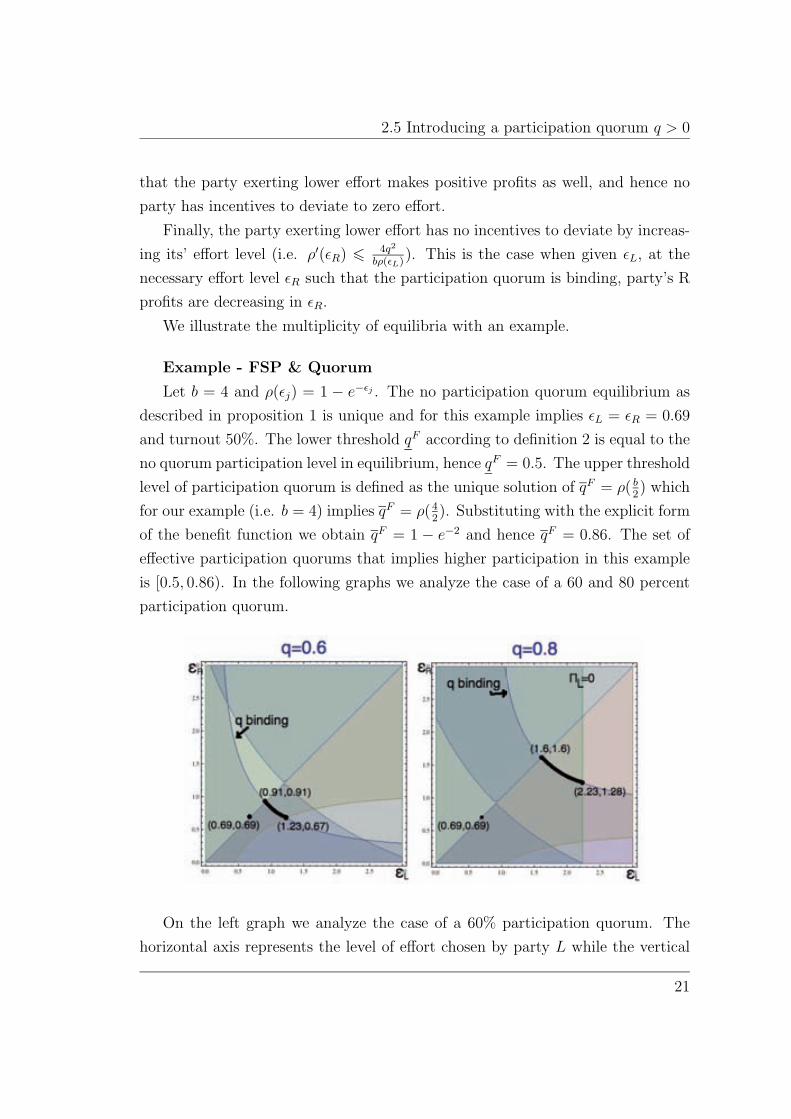
is [0.5, 0.86). In the following graphs we analyze the case of a 60 and 80 percent
participation quorum.
On the left graph we analyze the case of a 60% participation quorum. The
horizontal axis represents the level of effort chosen by party L while the vertical
21
Engineering Electoral Systems to Increase Turnout
axis represents the level of e�ort chosen by party R. The point (0:69; 0:69) is the
unique no quorum equilibrium. The downward slope curve depicts all the combi-
nations of �R and �L such that the participation quorum is binding. The unique
symmetric 60% participation quorum equilibrium is (0:91; 0:91). As expected un-
der the presence of a participation quorum parties have to increase their e�ort in
order to ful�ll it.
The bold part of the binding quorum curve depicts all the possible asymmetric
equilibria that satisfy the three conditions of proposition 8 and �L > �R. The point
(1:23; 0:67) is the most \asymmetric" among all asymmetric equilibria. This is
because if �L > 1:23 and the quorum is binding then d�Rd�R
> 0 (i.e. �0(�R) > 4q2
b�(�L)).
Hence, party R has incentives to deviate.
The case of a 80% participation quorum is depicted on the right graph. The
unique symmetric 80% participation quorum equilibrium is (1:6; 1:6). As expected
parties have to increase their e�ort in order to ful�ll the 80% participation quorum
more than in the case of the 60% quorum. Among all the asymmetric equilibria the
most \asymmetric" is the pair (2:23; 1:28). In contrast to the 60% participation
quorum, now the reason why �L can not be higher is that if �L > 2:23 and the
quorum binding then �L < 0 (i.e. �L >b�(�L)
2q).
In case of symmetric equilibria parties' pro�ts are decreasing in the level of
the participation quorum. Regarding asymmetric equilibria, in all cases of the
60% participation quorum, the party exerting higher e�ort (i.e. party L) makes
higher pro�ts. The relationship though, is exactly the opposite in the asymmetric
equilibria of the 80% participation quorum. In this case the party exerting lower
e�ort (i.e. party R) makes higher pro�ts. When the participation quorum is high,
in case of asymmetric equilibria there seems to be a free riding issue, while this is
not the case when the participation quorum is low.
Under a VSP there may exist multiple equilibria as described in the following
proposition.
Proposition 9. Under a VSP, for all b and all q 2 (qV ; qV ), (�L; �R) is an equi-
librium if and only if:
1. vL(�L) + vR(�R) = q
22
2.5 Introducing a participation quorum q > 0
2. �L <b�(�L)
2
3. �L > �R > �V (b)
According to the above proposition, in any equilibrium the quorum is binding
(i.e. vL(�L) + vR(�R) = q). Second, the party performing lower e�ort has to make
positive pro�ts (i.e. �L <b�(�L)
2). Third, the lower party's e�ort is equal or higher
than the no quorum VSP equilibrium e�ort level �V (i.e. �R > �V (b)). Notice that
the the symmetric equilibrium as described in proposition 7 satis�es all the three
conditions.
Claim 7. In case of a VSP in all asymmetric equilibria party R makes higher
profits than party L (free riding).
The party exerting lower e�ort free rides and makes higher pro�ts. This is
not always the case in the asymmetric equilibria under a FSP where which party
makes higher pro�ts actually depends on the level of the quorum. To illustrate
the multiplicity of equilibria we again proceed with an example.
Example - VSP & Quorum
As in the example of a FSP we assume that b = 4 and �(�j) = 1 � e��j . The
VSP no participation quorum equilibrium as described in the above proposition
is unique and implies �L = �R = 0:69 and turnout 50%. The lower threshold qF is
equal to the participation, hence qV = 0:5. In order to �nd the upper threshold we
�rst calculate the maximum e�ort level that each party may exert. �V;max is the
unique solution of b2�(�V;max) � �V;max = 0 and by substituting b and the explicit
form of function �(�j) we obtain 42(1 � e��V,max) � �V;max = 0. Solving for �V;max
we obtain that �V;max = 1:6. By de�nition 3 we obtain that qV = �(�V;max) = 0:8.
The set of e�ective participation quorums that implies higher participation in this
example is [0:5; 0:8). In the following graphs we analyze the case of a 60 and 80
percent participation quorum.
23

Engineering Electoral Systems to Increase Turnout
On the left graph we analyze the case of a 60% participation quorum. The
point (0.69, 0.69) is the unique no quorum equilibrium. The downward curve de-
picts all the combinations of εR and εL such that the participation quorum is bind-
ing. The unique symmetric 60% participation quorum equilibrium is (0.91, 0.91).
As expected, under the presence of a participation quorum, parties increase their
effort in order to fulfill it.
The bold part of the binding quorum curve depicts all the possible asymmetric
equilibria that satisfy the three conditions of proposition 9 and εL > εR. The point
(1.21, 0.69) is the most “ asymmetric” among all asymmetric equilibria since for
every point that εL > 1.21 and the quorum binding it is the case that party R has
incentives to deviate to εR = 0.69.
The case of an 80% participation quorum is depicted on the right graph. The
unique symmetric 80% participation quorum equilibrium is (1.6, 1.6). As expected
parties have to increase their effort even more in order to fulfill the 80% partici-
pation quorum. In this case there are no asymmetric equilibria since the partici-
pation quorum is equal to the upper threshold and both parties make zero profits.
As in the case of a FSP in case of the symmetric equilibria parties’ profits are
decreasing in the participation quorum level. The difference to the FSP system is
that in all asymmetric equilibria party R free rides and makes higher profits than
party L.
24
2.6 Discussion of the Voters' Decision
2.6 Discussion of the Voters’ Decision
In group turnout models (Shachar and Nalebu�, 1999; Herrera and Mattozzi,
2009) each voter reacts to his favorite party's e�ort and once the exerted e�ort
is high enough to compensate the voter's personal cost of voting, then the voter
rewards the party by voting for it. In general in group turnout models the ideology
of both parties and voters is not considered in detail. In this section we provide
an interpretation of why e�ort may mobilize voters in a spatial setup.
Let the society be split into two groups of voters each of them supporting one
of the two parties. For each group, voters' ideal points are uniformly distributed
on any closed interval of length two. Supporters of each party decide whether to
support their favorite party or to abstain. Each party's announced platform is
the mean of the distribution of the ideal points of its' supporters.
Formally, let xi denote voter's i ideal point and be uniformly distributed on
[� � 1; � + 1] while xj = � denotes party's j announced platform. Let �j 2 [0; 1]
be the e�ort exerted by party j. Voter i supporting party j obtains utility Ui =
�j � (xi � xj)2 if he participates in the election and votes for his favorite party j
and zero if he decides to abstain.
The above utility speci�cation implies that voter i participates in the election
and votes for his favorite party if and only ifp�j > (xi � xj). Remember that
according to the group-turnout model a voter participates in the election if and
only if �(�j) > ci. By de�ning c = jxi � xjj and function �(�j) =p�j the voters'
decision of the spatial model is equivalent to the voters' decision in the group-
turnout model. Notice that c and �(�j) satisfy all the assumptions of our model.
As in a group-turnout model, by de�ning �(�j) =p�j, the bene�t of each
voter is associated with the e�ort exerted by his favorite party. By de�ning that
c = jxi� xjj, in this spatial setup the personal cost of each voter is interpreted as
the cost of supporting a party further from own's own ideal point.
25

Engineering Electoral Systems to Increase Turnout
Figure 2: A spatial Interpretation of Group-Turnout Models
As we see from figure two, in the spatial setup, as in the group-turnout model,
turnout is increasing in effort. Actually, in the spatial setup, effort is the way to
attract voters that are not so close to the platform of their favorite party. This is
because, voters that have policy preferences different from the platform of their
favorite party are willing to participate in the election if their favorite party’ s
effort is high enough, such that it compensates the cost of supporting a policy
further from their own ideal point.
2.7 Conclusion
In this paper we study the effect of different instruments that increase turnout
in PR elections. We find that the introduction of a VSP system has a positive
effect on turnout as long as parties obtain high benefits for being in office, while
the establishment of certain participation quorums can always boost turnout.
In terms of welfare and in line with our model, if the utility of a voter is
defined as the benefit a voter obtains as a result of the effort exerted by his favorite
26
2.7 Conclusion
party minus the personal cost of voting, then an increase in turnout through the
introduction of a VSP or a participation quorum increases voters welfare. This
is a consequence of the higher levels of turnout as a result of the higher e�ort
exerted by parties in equilibrium in an expressive voting model.
We �nd that our mechanisms dominate compulsory voting in terms of voters'
welfare. If we were to introduce compulsory voting in our model, in equilibrium
parties would exert zero e�ort since they would not have incentives to exert any
e�ort in order to mobilize their voters to participate. This is because in our
model we do not allow a \none of the above" option and when voters are forced
to participate they would support their favorite party even when the latter does
not exert any e�ort at all. Hence, compulsory voting would imply negative total
welfare for voters, since all voters would obtain negative utility given that parties
would not exert any e�ort at all while all voters would have to pay the cost of
participating or the cost of a penalty in case they would decide to abstain.
The advantage of the electoral rules we propose over compulsory voting as a
solution to low turnout is that they increase the e�ort put by parties in order
to convince voters to participate. In other words, and in contrast to compulsory
voting, our mechanisms target one of the underlying reasons of low turnout (i.e.
low e�ort) rather than only the result itself (i.e. participation level).
A common feature of the two mechanisms we propose is that when appro-
priately used they increase turnout and at the same time they decrease parties'
welfare. This result may explain why parties often target to increase turnout
through other alternatives such as organizing simultaneous elections, facilitating
voters' registration, switching the election to a weekend day or allowing absen-
tee voting7. All these alternatives are costless for parties. They indeed increase
turnout by reducing the cost of voting. At the same time and in contrast to
our mechanisms they do not decrease parties' bene�ts. Hence, even when parties
recognize the need for higher turnout, given that they have the power over in-
stitutional changes, probably they will keep aiming to increase turnout through
such alternatives.
Our results may as well explain the evolution of a participation quorum sys-
7See Wattenberg (1998); Blais et al. (2003); Geys (2006) for empirical evidence.
27

Engineering Electoral Systems to Increase Turnout
tem in several post-Soviet states8. As we have shown a participation quorum is
associated with higher levels of turnout. This exactly was the reason why the
participation quorum had been established in these countries right after the fall
of Communism. The target of the electoral designers was to guarantee the legit-
imacy of the new form of government through high levels of turnout. Moreover,
we have shown that parties' pro�ts are decreasing in the level of the participation
quorum. This may explain why with the passage of time and the strengthen of
political parties, the participation quorum has been abolished or even modi�ed to
a lower level.
In well established democracies turnout levels are often decreasing. One of
the common justi�cations for this, is that voters are tired of the existing political
parties, elections and politics in general. According to our results parties and
voters have interests in con ict. Hence, voters' apathy may not stem from voters'
fatigue per se, rather than the fact that parties' pro�ts are higher when citizens
remain uninvolved.
8While a fifty percent quorum is still present in the cases of Moldova and Hungary, in Serbiaand Ukraine the quorum has been abolished. Ukraine did so for the 1998 elections after theexperience of repeated by-elections failing to reach the required turnout in 1994. Serbia abolishedthe quorum in 2004 since it had not been met and no president had been elected during twoyears and three elections. In Macedonia in 2009 the president decided to decrease the minimumlevel of participation from a 50% to a 40% probably to prevent the possibility of a new election.
28
2.8 Appendix
2.8 Appendix
Proof of Proposition 1
Parties maximize pro�ts. The optimization problem of party L is:
Max.fbsL � �Lg and by substituting sL:
Max:fb ��(�L)��(�L)+(1��)�(�R)
� �Lg
Taking F.O.C. with respect to e�ort for party L we obtain that it has to hold:
�(1� �)�(�R)�0(�L)
[��(�L) + (1� �)�(�R)]2=
1
b(2.1)
Solving the same problem for party R we get:
�(1� �)�(�L)�0(�R)
[��(�L) + (1� �)�(�R)]2=
1
b(2.2)
From equations (1) and (2) in equilibrium it has to hold that:
�(�R)�0(�L)
�(�L)�0(�R)= 1
which implies that in equilibrium:
�0(�L)
�(�L)=�0(�R)
�(�R)(2.3)
Notice that�0(�j)�(�j)
is strictly decreasing in �j for all �j > 0. This is because of
the strict monotonicity and strict concavity of function �(�j). More speci�cally
we have:d�0(�j)�(�j)
d�j=�00(�j)�(�j)� �0(�j)�0(�j)
[�(�j)]2< 0
Given that�0(�j)�(�j)
is strictly decreasing in �j and equation (3) in equilibrium
it hold that �FR = �FL = �F . By substituting �FR = �FL = �F in equation (1) or
(2) we obtain that both parties exert the same amount of e�ort that satis�es the
29
Engineering Electoral Systems to Increase Turnout
equilibrium condition:�0(�F )
�(�F )=
1
b�(1� �)(2.4)
In order to guarantee that �F is the equilibrium e�ort level it has to be the
case that both parties make positive pro�ts. Party L makes pro�ts: �FL =
b ��(�F )��(�F )+(1��)�(�F )
� �F = b� � �F . Party R makes pro�ts �FR = b(1 � �) � �F .
Given that � 2 [0:5; 1) it holds that �FL > �FR . In order to guarantee that both
parties make positive pro�ts it is enough to show that �FR > 0. From the pro�t
function �FR > 0 is true if �F < b(1 � �). Because of the concavity of �(�j) it
holds that �F < �(�F )�0(�F )
and from (4) this implies that �F < �(1� �)b. Given that
� < 1, the latter implies that �FR > 0 and hence in equilibrium both parties make
positive pro�ts for whatever values of � and b.
Proof of Proposition 2
From the equilibrium condition (4) if b increases then �0(�F )�(�F )
decreases. Given
that �0(�F )�(�F )
is strictly decreasing in �j, we conclude that �F is strictly increasing in
b.
If � increases then 1�(1��)b
increases. Again from (4), this implies that �0(�F )�(�F )
increases and hence �F is strictly decreasing in �.
Proof of Claim 1
Party L makes pro�ts: �FL = b ��(�F )��(�F )+(1��)�(�F )
� �F = b�� �F .
Party R makes pro�ts �FR = b(1� �)� �F .
Given that � 2 [0:5; 1) it holds that �FL > �FR with the equality holding for
� = 0:5.
Proof of Proposition 3
Party L solves: Max.fb��(�L) � �Lg. Taking F.O.C. with respect to �L we
obtain that the solution has to satisfy:
�0(�VL ) =1
b�(2.5)
Notice that since �(�j) is strictly concave then the solution of the maximization
is unique.
30
2.8 Appendix
Performing the same maximization for party R we obtain that:
�0(�VR) =1
b(1� �)(2.6)
In order to guarantee that �VL and �VR are part of an equilibrium both parties have
to make positive pro�ts. Because of the strict concavity of �(�j) it holds that
�VL <�(�VL )
�0(�VL )and from equation (5), �VL < b��(�VL ). Given that �VL = b��(�VL ) � �VL
we conclude that �VL > 0. In the same way for party R, �VR <�(�VR)
�0(�VR)which implies
that �VR < b(1� �)�(�VR) and hence �VR > 0.
If � = 0:5 then �VL = �VR = �V . If � > 0:5 then � > 1 � � which implies that1b�< 1
b(1��)which implies that �0(�VL ) < �0(�VR) and because of the strict concavity
of �(�j) this implies that �VL > �VR.
Proof of Proposition 4
From equilibrium condition (5) we know that �0(�VL ) = 1b�
and from (6) that
�0(�VR) = 1b(1��)
.
If b increases then both �0(�VL ) and �0(�VL ) decrease. Because of the strict
concavity of �(�j) this implies that both �VL and �VR are strictly increasing in b.
If � increases then from (5) �0(�VL ) decreases and from (6) �0(�VL ) increases.
Because of the strict concavity of �(�j) this implies that �VL is strictly increasing
in � while �VR is strictly decreasing in �.
Proof of Claim 2
Pro�ts are given by the following expressions: �VL = b��(�VL ) � �VL and �VR =
b(1� �)�(�VR)� �VR.
If � = 0:5 then from equilibrium conditions (5) and (6) it holds that �VL =
�VR = �V and hence �VL = �VR .
If � > 0:5 then from proposition 3 it holds that �VL > �VR. Because of the strict
concavity of �(�j) it holds that �0(�VL ) <�(�VL )��(�VR)
�VL��VR
which is equivalent to:
�VL � �VR <�(�VL )� �(�VR)
�0(�VL )(2.7)
In order be true that �VL > �VR it must hold that b��(�VL )��VL > b(1��)�(�VR)��VR
31
Engineering Electoral Systems to Increase Turnout
which is equivalent to:
�VL � �VR < b��(�VL )� b(1� �)�(�VR) (2.8)
Given that inequality (7) always holds in order to show that �VL > �VR it is enough
to show that the RHS of inequality (7) is smaller than the RHS of equation (8).
Hence we have to show that�(�VL )��(�VR)
�0(�VL )< b��(�VL )�b(1��)�(�VR). By substituting
�0(�VL ) = 1�b
we obtain that it has to hold b�[�(�VL ) � �(�VR)] < b��(�VL ) � b(1 ��)�(�VR) or b(1 � �)�(�VR) < b��(�VR) which is equivalent to 1 � � < � and the
latter is true given that � > 0:5. Hence, if � < 0:5 then �VL > �VR .
Proof of Proposition 5
From equilibrium conditions 4 and 5 we get that for party L it holds that
�0(�VL ) = 1b�
and �0(�F )�(�F )
= 1b�(1��)
. Combining the two we obtain that�0(�VL )
1�� = �0(�F )�(�F )
which is equivalent to:
�0(�VL )
�0(�F )=
1� ��(�F )
(2.9)
From condition (9) and the strict concavity of �(�j) we obtain that:
� �VL = �F if and only if �(�F ) = 1� �. The latter holds if and only if b = b.
� �VL > �F if and only if�0(�VL )
�0(�F )< 1 which is true if and only if 1��
�(�F )< 1 thus if
and only if �(�F ) > 1� �. The latter is true if and only if b > b.
� In the same way, �VL < �F if and only if b < b.
Performing the same approach for party R, we obtain that �VR = �F if and only if
b = b, �VR > �F if and only if b > b and �VR < �F if and only if b < b.
Proof of Proposition 6
We analyze all possible symmetric pure strategy Nash equilibria where both
parties exert the same level of e�ort �L = �R. Those can belong in the following
categories:
1. vL + vR > q (i.e. the quorum is slack)
2. vL + vR = q (i.e. the quorum is binding)
32
2.8 Appendix
3. vL + vR < q (i.e. the quorum is not ful�lled)
In general our approach is the following. For each pair of levels of e�ort (�L; �R)
we have to guarantee that there are no incentives for any of the parties to deviate.
Hence, if e�ort level �j is part of a Nash equilibrium it has to be the solution of the
(constrained) maximization problem of party j given the e�ort of the opponent
��j. Moreover, we have to guarantee that each e�ort level being part of a Nash
equilibrium implies positive pro�ts given that the deviation �j = 0 implying zero
pro�ts is always available.
1. Participation quorum slack.
Let �L = �R = � be such that vL + vR > q.
Given �R = � the maximization problem of party L is:
Max.fb �(�L)�(�L)+�(�)
� �Lg subject to vL + vR > q and by substituting the vote
shares in the constraint this is equivalent to:
Max.fb �(�L)�(�L)+�(�)
� �Lg subject to �(�L) + �(�) > 2q
The Lagrangian of this problem is:
L = b �(�L)�(�L)+�(�)
� �L + �[�(�L) + �(�)� 2q]
Taking F.O.C. with respect to �L we obtain:
L�L = b �′(�L)�(�)[�(�L)+�(�)]2
� 1 + ��0(�L)
If �L = � is part of the equilibrium it must satisfy the F.O.C. of party L.
Given that the participation quorum is slack, this means that the associated
multiplier is zero (i.e. � = 0). Hence If �L = � is part of the equilibrium it
must be true that:
b �′(�)�(�)[�(�)+�(�)]2
� 1 = 0 which implies that �′(�)�(�)
= 4b. Notice that the unique
solution of �′(�)�(�)
= 4b
is � = �F which is unique FSP no quorum equilibrium
e�ort level for � = 0:5.
In order the constraint to be slack it must be that that the level of partici-
pation is higher than the quorum. This is the case when �(�F ) > q which is
equivalent to qF > q.
33

Engineering Electoral Systems to Increase Turnout
In order to guarantee positive pro�ts it must hold that �L = b2� �F > 0.
This is true if �F < b2.
Because of the strict concavity of � it holds that �0(�F ) < �(�F )�F
which is
equivalent to �F < �(�F )�′(�F )
thus �F < b4. Hence, �F < b
2and this implies that
party L makes positive pro�ts.
The same applies for party R.
Hence, �L = �R = �F such that �′(�F )�(�F )
= 4b
is an equilibrium if q < qF
2. Participation Quorum Binding
Let �L = �R = �F;q be such that vL + vR = q.
Given e�ort �R = �F;q the maximization problem of party L is:
Max.fb �(�L)�(�L)+�(�F,q)
� �Lg subject to vL + vR > q
Given that with e�ort �R = �F;q party R ful�lls half of the quorum (i.e.
vR = 12�(�F;q) = 1
2q), the problem can be written as:
Max.fb �(�L)�(�L)+�(�F,q)
� �Lg subject to �(�L) > q
The Lagrangian of this problem is:
L = b �(�L)�(�L)+�(�F,q)
� �L + �[�(�L)� q]
Taking F.O.C. with respect to e�ort we obtain:
L�L = b�′(�L)�(�F,q)[�(�L)+q]2
� 1 + ��0(�L)
If �L = �F;q > 0 is the best response it must hold that b�′(�F,q)�(�F,q)[2�(�F,q)]2
� 1 +
��0(�F;q) = 0. Solving for the Lagrange multiplier we obtain that � =1
�′(�F,q)� b
4�(�F,q). Given that the constraint is binding it has to be that � > 0
which is true if and only if �0(�F;q) 6 4�(�F,q)b
which is true if �′(�F,q)�(�F,q)
6 �′(�F )�(�F )
or �F;q > �F i.e. �(�F;q) > �(�F ) and hence � > 0 if q > qF .
Last we have to guarantee that pro�ts are positive which holds if �F;q < b2
i.e. q < qF . By symmetry the same applies for party R.
3. Participation Quorum not Ful�lled.
34

2.8 Appendix
� �L = �R = � > 0
Given that the participation quorum is not satis�ed and parties exert
positive e�ort, parties make negative pro�ts �j = �� < 0. Hence (�; �)
can not be an equilibrium given that party j has incentives to deviate
to zero e�ort and zero pro�ts respectively.
� �L = �R = 0
Given ��j = 0 for whatever positive e�ort party j obtains all the seats in
the parliament if the participation quorum is ful�lled. The constrained
maximization problem of party j is: Max.fb��jg subject to �(�j) > 2q.
The solution of this problem is �qj such that �(�qj) = 2q. Notice that �qjis the e�ort level required by party j in order to ful�ll the quorum by
itself. Finally, in order party j to deviate to e�ort �qj it has to be that it
makes positive pro�ts. This is the true if �qj < b. If the latter inequality
does not hold then �j = 0. Hence, �L = �R = 0 is an equilibrium if
�qj > b.
Summing up the cases regarding symmetric equilibria we have obtained:
1. �L = �R = �F such that �′(�F )�(�F )
= 4b
is an equilibrium if q < qF
2. �L = �R = �F;q such that �(�F;q) = q is an equilibrium if qF 6 q < qF
3. �L = �R = 0 is an equilibrium if �qj > b where �qj is the unique solution of
�(�qj) = 2q
Hence if q < qF then we fall in case 1. If qF 6 q < qF then we fall in case 2.
Finally if q > qF then �qj > b which is the condition for case 3.
�qj > b is true since q > qF implies that �(�F;qj ) > �( b2) which implies that
�F;qj >b
2(2.10)
Moreover it holds that �qj > �F;qj which implies that�(�qj )
�qj<
�(�F,qj )
�F,qji.e. 2q
�qj< q
�F,qjwhich is equivalent to:
�F;qj <�qj2
(2.11)
35

Engineering Electoral Systems to Increase Turnout
Combining the inequalities (10) and (11) we have shown that if q > qF then
�qj > b and hence if q > qF then from case 3 the equilibrium is �L = �R = 0.
Proof of Claim 3
As we have shown in the proof of proposition 1, for � = 12
it holds that
�F (b) < b4. Given that function � is strictly increasing this implies that the set
[�(�F (b)); �( b2)) is not-empty.
Proof of Claim 4
As we have shown in proposition 2 participation in a FSP with no participation
quorum is increasing in the bene�t parties obtain. Given that the lower threshold
is de�ned as the no quorum participation level, then qF (b) is increasing in the
bene�t as well.
The upper threshold is de�ned as qF = �( b2). Given that the bene�t function
� is strictly increasing in b then qF (b) is strictly increasing in b.
Proof of Proposition 7
We analyze all possible pure strategy symmetric Nash equilibria where �L = �R.
Those can belong in the following categories:
1. vL + vR > q (i.e. the quorum is slack)
2. vL + vR = q (i.e. the quorum is binding)
3. vL + vR < q (i.e. the quorum is not ful�lled)
1. Participation quorum is slack
Let �L = �R = � be such that vL + vR > q.
Given e�ort �R = � the maximization problem of party L is:
Max.f12b�(�L)� �Lg subject to �(�L) + �(�) > 2q
The Lagrangian of this problem is:
L = 12b�(�L)� �L + �[�(�L) + �(�)� 2q]
Taking F.O.C. with respect to e�ort we obtain:
L�L = 12b�0(�L)� 1 + ��0(�L)
36
2.8 Appendix
Given the participation quorum is slack the associated Lagrange multiplier
takes value zero (i.e � = 0). Hence, if �L = � is part of the equilibrium it
must satisfy:
�0(�L) = 2b
which is the no quorum equilibrium condition and hence �L = �V .
In order the constraint to be slack it must be that �(�V ) > q which is
equivalent to qV > q.
In order to guarantee positive pro�ts it must be that �V < 12b�(�V ). Because
of the strict concavity of � it holds that �0(�V ) < �(�V )�V
which implies that
�V < �(�V )�′(�V )
and by substituting �0(�V ) = 2b
we obtain that it holds that
�V < 12b�(�V ). Hence, pro�ts are positive.
The same applies for party R.
2. Participation quorum is binding:
Let �L = �R = �V;q be such that vL + vR = q
Given e�ort �R = �V;q the Lagrangian of this problem is:
L = 12b�(�L)� �L + �[�(�L) + �(�V;q)� 2q]
Taking F.O.C. with respect to e�ort we obtain:
L�L = 12b�0(�L)� 1 + ��0(�L)
If �L = �V;q > 0 is the solution it must hold that 12b�0(�V;q)�1+��0(�V;q) = 0.
Given that the constraint is binding it has to be that � > 0 which is true
if �0(�V;q) 6 2b
and by substituting 2b
= �0(�V ) we obtain �0(�V;q) 6 �0(�V )
which is true if �V;q > �V i.e. �(�V;q) > �(�V ) or q > qV .
Finally it has to be that pro�ts are positive which holds if �V;q < 12b�(�V;q)
which is true if q < qV . The same applies for party R.
3. Participation Quorum not Ful�lled
Let �L = �R = � > 0 be such that vL + vR < 0.
Party j makes pro�ts �j = �� < 0. Hence �L = �R = � > 0 can not be an
equilibrium given that party j has incentives to deviate to �j = 0.
Let �L = �R = 0 be such that vL + vR < 0.
37

Engineering Electoral Systems to Increase Turnout
This can be an equilibrium if no party can ful�ll the quorum by itself and
make positive pro�ts.
Let �qj be such that �(�qj) = 2q. Notice that �qj is the e�ort level required by
party j in order to ful�ll the quorum by itself. In order to guarantee that
pro�ts are positive it must hold that �qj <12b�(�qj). If the later inequality does
not hold then �j = 0. Hence, �L = �R = 0 is an equilibrium if �qj > 12b�(�qj)
i.e. �qj > �V;max i.e. �(�qj) > �(�V;max) i.e. q > qV .
Summing up the cases regarding pure strategy symmetric Nash equilibria un-
der a VSP we have obtained:
1. �L = �R = �V such that �0(�V ) = 2b
is an equilibrium if q < qV .
2. �L = �R = �V;q such that �(�V;q) = q is an equilibrium if qV 6 q < qV .
3. �L = �R = 0 is an equilibrium if q > qV .
Proof of Claim 5
As we have shown participation in a VSP with no participation quorum is
strictly increasing in the bene�t parties obtain. Given that the lower threshold is
de�ned as the no quorum participation level, then qV (b) is strictly increasing in
the bene�t as well.
The upper threshold is de�ned as qV = �(�V;max), where �V;max is the unique
solution of F = 12b�(�V;max)� �V;max = 0. From the implicit function theorem we
know thatd�V;max
db= �
dFdbdF
d�V,max
= ��(�V,max)
2b2�0(�V;max)� 1
(2.12)
Given that �V;max > �V then it holds that b2�0(�V;max)� 1 < 0 and hence d�V,max
db>
0. Moreover given that qV = �(�V;max) and �(�j) is strictly increasing in �j we
conclude that qV is strictly increasing in b.
Proof of Claim 6
� The lower thresholds are de�ned as equilibrium turnout in the no quorum
case. As we have shown in Proposition 5 for the case of � = 12
there exists
38

2.8 Appendix
a unique b� such that turnout under a FSP and a VSP is the same. Hence
if b = b� then qV (b) = qF (b). If b > b� then turnout under a VSP is higher
and hence qV (b) > qF (b). If b < b� then turnout under a VSP is lower and
hence qV (b) < qF (b).
� By de�nition qF > qV if �( b2) > �(�V;max) which is true if b
2> �V;max and
given that �V;max = 12b�(�V;max) the latter inequality is equivalent to b
2>
b2�(�V;max). The latter holds since �(�V;max) < 1 for all �nite b and hence
qF > qV .
Proof of Proposition 8
We analyze all possible asymmetric Nash equilibria where without loss of gen-
erality �L > �R. Those can belong in the following categories:
1. vL + vR > q (i.e. the quorum is slack)
2. vL + vR = q (i.e. the quorum is binding)
3. vL + vR < q (i.e. the quorum is not ful�lled)
1. Participation Quorum Slack
Let �L > �R be such that vL + vR > q.
Given e�ort �R the maximization problem of party L is:
Max.fb �(�L)�(�L)+�(�R)
� �Lg subject to �(�L) + �(�R) > 2q
The Lagrangian of this problem is:
L = b �(�L)�(�L)+�(�R)
� �L + �L[�(�L) + �(�R)� 2q]
Taking F.O.C. with respect to e�ort we obtain:
L�L = b �′(�L)�(�R)[�(�L)+�(�R)]2
� 1 + �L�0(�L)
Given that the constraint is slack then it holds that �L = 0. Then it has to
hold that: b �′(�L)�(�R)[�(�L)+�(�R)]2
� 1 = 0.
In the same way for party R it has to hold that: b �′(�R)�(�L)[�(�L)+�(�R)]2
� 1 = 0.
39
Engineering Electoral Systems to Increase Turnout
Combining the above two it has to be true that �′(�L)�(�L)
= �′(�R)�(�R)
which as we
have shown is true only for �L = �R. Hence, contradiction. �L > �R such
that vL + vR > q can not be an equilibrium.
2. Participation Quorum Binding
Let �L > �R be such that vL + vR = q.
Given e�ort �R the maximization problem of party L is:
Max.fb �(�L)�(�L)+�(�R)
� �Lg subject to �(�L) + �(�R) > 2q
The Lagrangian of this problem is:
L = b �(�L)�(�L)+�(�R)
� �L + �L[�(�L) + �(�R)� 2q]
Taking F.O.C. with respect to e�ort we obtain:
L�L = b �′(�L)�(�R)[�(�L)+�(�R)]2
� 1 + �L�0(�L)
In order the participation quorum to be binding it must be the case that
q > �(�F ) i.e. q > qF .
Given the participation quorum is binding it must be that �L > 0. This is
true if and only if �0(�L) 6 4q2
b�(�R).
Performing the same maximization problem for party R we obtain that
�R > 0 if and only if �0(�R) 6 4q2
b�(�L).
Notice that since �L > �R it holds that �0(�L) < �0(�R) and 4q2
b�(�L)< 4q2
b�(�R).
Hence �0(�R) 6 4q2
b�(�L)is su�cient to guarantee that both �L and �R are
positive.
In order to guarantee positive pro�ts for both parties it must hold that �L <b�(�L)
2qand �R <
b�(�R)2q
. Notice that since �L > �R it holds that �(�L)�L
< �(�R)�R
.
Hence, �L <b�(�L)
2qis su�cient to guarantee that both parties make positive
pro�ts.
3. Participation Quorum not Ful�lled
Let �L > �R > 0 be such that vL + vR < 0.
Party L makes negative pro�ts �L = ��L < 0. Hence it can not be an
equilibrium given that it has incentives to deviate to � = 0
40
2.8 Appendix
Proof of Proposition 9
We analyze all possible pure strategy asymmetric Nash equilibria where with-
out loss of generality �L > �R. Those can belong in the following categories:
1. vL + vR > q (i.e. the quorum is slack)
2. vL + vR = q (i.e. the quorum is binding)
3. vL + vR < q (i.e. the quorum is not ful�lled)
1. Participation Quorum Slack
Let �L > �R be such that vL + vR > q.
Given e�ort �R the maximization problem of party L is:
Max.f12b�(�L)� �Lg subject to �(�L) + �(�R) > 2q
The Lagrangian of this problem is:
L = 12b�(�L)� �L + �[�(�L) + �(�R)� 2q]
Taking F.O.C. with respect to e�ort we obtain:
L�L = 12b�0(�L)� 1 + ��0(�L)
Given the participation quorum is slack the associated Lagrange multiplier
takes value zero (i.e � = 0). As before for � = 0 we would get that for party
L it should hold that: �0(�L) = 2b.
Performing the same maximization problem for party R we obtain that it
should hold that �0(�R) = 2b.
Combining the two it has to be true that �0(�L) = �0(�R) which because of
the strict concavity of �(�j) is true if and only if �L = �R.
Hence, �L > �R such that vL + vR > q can not be an equilibrium.
2. Participation Quorum Binding
Let �L > �R be such that vL + vR = q
Given e�ort �R the Lagrangian of the maximization problem of party L is:
41

Engineering Electoral Systems to Increase Turnout
L = 12b�(�L)� �L + �[�(�L) + �(�R)� 2q]
Taking F.O.C. with respect to e�ort we obtain:
L�L = 12b�0(�L)� 1 + ��0(�L)
If �L is part of an equilibrium it has to hold that 12b�0(�L)� 1 + ��0(�L) = 0.
Given that the participation quorum is binding it must be that � > 0 which
is true if and only if �0(�L) 6 2b
which is equivalent to �0(�L) 6 �0(�V ) i.e.
�L > �V .
Performing the the same maximization problem for party R we obtain that
it has to hold that �R > �V .
In order to guarantee positive pro�ts for party L it has to be that �L <b�(�L)
2
i.e.�(�L)�L
> 2b. For party R it has to hold that �R <
b�(�R)2
i.e. �(�R)�R
> 2b.
Given that �L > �R and because of the strict concavity of the � function
it holds that �(�R)�R
> �(�L)�L
. Hence in order to guarantee positive pro�ts for
both parties it is su�cient that �L <b�(�L)
2.
3. Participation Quorum not Ful�lled
Let �L > �R > 0 be such that vL + vR < 0.
Party L makes negative pro�ts �L = ��L < 0. Hence it can not be an
equilibrium given that it has incentives to deviate to � = 0
Proof of Claim 7
For the pro�t function under a VSP it holds that:
@�V
@�j=
1
2b�0(�j)� 1 (2.13)
and@2�V
@�2j=
1
2b�00(�j) < 0 (2.14)
Hence, pro�ts under a VSP are strictly concave in e�ort. Given that in asymmetric
equilibria it holds that �L > �R > �V where �V is the e�ort that maximizes pro�ts
42
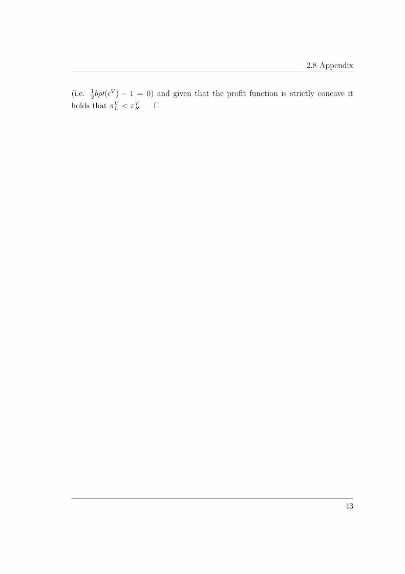
2.8 Appendix
(i.e. 12b�0(�V ) � 1 = 0) and given that the pro�t function is strictly concave it
holds that �VL < �VR .
43
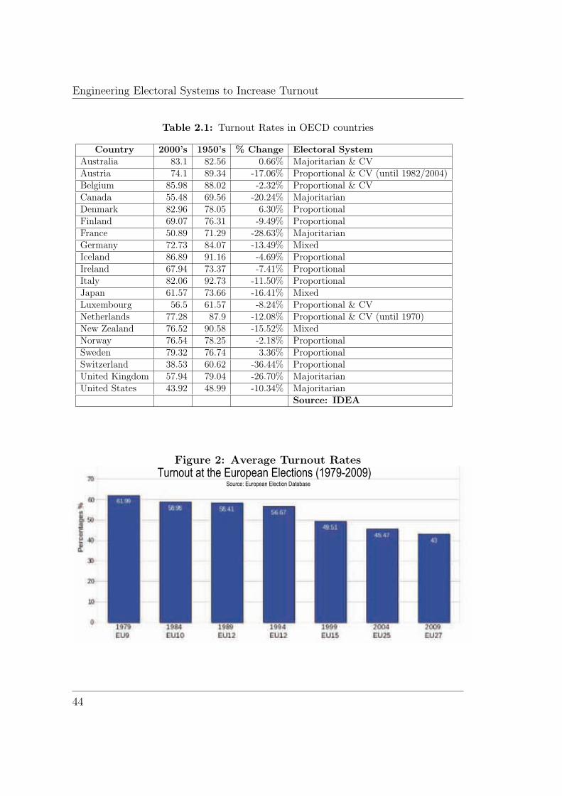
Engineering Electoral Systems to Increase Turnout
Table 2.1: Turnout Rates in OECD countries
Country 2000’s 1950’s % Change Electoral SystemAustralia 83.1 82.56 0.66% Majoritarian & CVAustria 74.1 89.34 -17.06% Proportional & CV (until 1982/2004)Belgium 85.98 88.02 -2.32% Proportional & CVCanada 55.48 69.56 -20.24% MajoritarianDenmark 82.96 78.05 6.30% ProportionalFinland 69.07 76.31 -9.49% ProportionalFrance 50.89 71.29 -28.63% MajoritarianGermany 72.73 84.07 -13.49% MixedIceland 86.89 91.16 -4.69% ProportionalIreland 67.94 73.37 -7.41% ProportionalItaly 82.06 92.73 -11.50% ProportionalJapan 61.57 73.66 -16.41% MixedLuxembourg 56.5 61.57 -8.24% Proportional & CVNetherlands 77.28 87.9 -12.08% Proportional & CV (until 1970)New Zealand 76.52 90.58 -15.52% MixedNorway 76.54 78.25 -2.18% ProportionalSweden 79.32 76.74 3.36% ProportionalSwitzerland 38.53 60.62 -36.44% ProportionalUnited Kingdom 57.94 79.04 -26.70% MajoritarianUnited States 43.92 48.99 -10.34% Majoritarian
Source: IDEA
Figure 2: Average Turnout RatesTurnout at the European Elections (1979-2009)
Source: European Election Database
44
BIBLIOGRAPHY
Bibliography
Blais, A. and A. Dobrzynska (1998): \Turnout in electoral democracies,"European Journal of Political Research, 33, 239{262.
Blais, A., L. Massicotte, and A. Dobrzynska (2003): \Why is turnouthigher in some countries than in others," Ottawa: Elections Canada.
Borgers, T. (2004): \Costly voting," American Economic Review, 94, 57{66.
Carrillo, J. and M. Castanheira (2008): \Information and Strategic Polit-ical Polarization," Economic Journal, 118, 845{874.
Colomer, J. M. (2004): Handbook of electoral system choice, Palgrave Macmil-lan.
Franklin, M. (1999): \Electoral engineering and cross-national turnout di�er-ences: what role for compulsory voting?" British Journal of Political Science.
||| (2004): Voter turnout and the dynamics of electoral competition in estab-lished democracies since 1945, Cambridge Univ Pr.
Gerardi, D., M. McConnell, J. Romero, and L. Yariv (2009): \GetOut the (Costly) Vote: Institutional Design for Greater Participation," CarloAlberto Notebooks.
Gerber, A. and D. Green (2000): \The e�ects of canvassing, telephone calls,and direct mail on voter turnout: A �eld experiment," American Political Sci-ence Review, 94, 653{663.
Gerber, A., D. Green, and C. Larimer (2008): \Social pressure and voterturnout: Evidence from a large-scale �eld experiment," American Political Sci-ence Review, 102, 33{48.
Geys, B. (2006): \Explaining voter turnout: A review of aggregate-level re-search," Electoral Studies, 25, 637{663.
45
BIBLIOGRAPHY
Ghosal, S. and B. Lockwood (2009): \Costly voting when both informationand preferences di�er: is turnout too high or too low?" Social Choice andWelfare.
Herrera, H. and A. Mattozzi (2009): \Quorum and turnout in referenda,"Journal of the European Economic Association.
Hirczy, W. (1994): \The impact of mandatory voting laws on turnout: A quasi-experimental approach* 1," Electoral Studies.
Jackman, R. (1987): \Political institutions and voter turnout in the industrialdemocracies," The American Political Science Review, 405{423.
Krasa, S. and M. K. Polborn (2009): \Is mandatory voting better thanvoluntary voting?" Games and Economic Behavior, 66, 275{291.
Lijphart, A. (1997): \Unequal participation: Democracy's unresolveddilemma," American Political Science Review.
Polo, M. (1998): \Electoral competition and political rents," IGIER e BocconiUniversity.
Shachar, R. and B. Nalebuff (1999): \Follow the leader: Theory and evi-dence on political participation," American Economic Review, 89, 525{547.
Snyder, J. (1989): \Election goals and the allocation of campaign resources,"Econometrica: Journal of the Econometric Society.
Wattenberg, M. (1998): The decline of American political parties, 1952-1996,Harvard Univ Pr.
46

Chapter 3
Participation Quorums in CostlyMeetings1
3.1 Introduction
In any kind of decision making processes where a participation quorum require-
ment applies, the decision is valid only if participation is higher than a given level.
Examples are various and include large elections such as referenda and presidential
elections, but even more frequently smaller scale decision making meetings such
as meetings of faculty members, shareholders, neighbors, or members of many
societies, and clubs2.
Although economists have extensively studied alternative voting rules, the use
of a participation quorum has received very little attention. Recently, di�erent au-
thors (Maniquet and Morelli, 2010; Herrera and Mattozzi, 2009; Aguiar-Conraria
and Magalh~aes, 2010a,b; Houy, 2009) have studied the e�ect of a participation
quorum in referenda. In this case, when not enough voters participate, the refer-
endum is considered to be invalid and the outcome is a reversal to the status quo.
On the contrary, in decision making meetings, in case the quorum is not ful�lled,
the meeting has to be repeated since a decision must be taken (i.e. in contrast to
the case of referenda there is no reversal to the status quo). The importance of
analyzing such a situation lies in the fact that, although such a participation re-
1This chapter is coauthored with Sabine Flamand2The voting procedure in shareholders’ meetings varies among most countries and is deter-
mined by each county’s corporate law (Dornseifer, 2005).
47
Participation Quorums in Costly Meetings
quirement is widely applied, as we show, it often has negative welfare implications,
including policy distortions.
We build on the model of costly meetings by Osborne et al. (2000)3. In the
general setup, which may apply to any meeting and which we refer to as the No-
Quorum Game, a group of individuals has to decide on a policy through a decision
making meeting. Each member of the group independently decides whether to
participate, at a cost, in the meeting, whose outcome is assumed to be a compro-
mise between the participants' favorite policies. In deciding whether to attend or
not, each member compares the cost of attending with the impact of her presence
on the policy decision.
Similar to Bulkley et al. (2001), we characterize the Nash equilibrium of the
one-shot attendance game by using a constructive approach as follows: We assume
a sequential exit process that starts with the full set of attendees, and at each step
of which the individual with the largest bene�t from not attending the meeting
is the one who exits. The process �nishes when no further attendee is willing
to exit. We fully characterize this exit process, and we argue that it ends at a
unique Nash equilibrium belonging to the set of equilibria of the original Osborne
et al. (2000) one-shot attendance game. Through this exit process, we are able
to characterize the unique Nash equilibrium of any such attendance game, which
consists in a set of attendees and the corresponding policy decision.
More importantly, in order to extend the attendance game to decision making
meetings for which a participation quorum applies (which we refer to as the quo-
rum game), we introduce two additional notions: the participation quorum itself,
and how much members are harmed by the fact that a decision is delayed in case
the meeting has to be postponed. Our ultimate goal is to analyze the e�ect of such
a participation quorum on the equilibrium set of attendees, the policy decision
and on total welfare.
As in Osborne et al. (2000), the equilibrium of the No-Quorum game that is
reached through the exit process is such that moderates tend to abstain, while
extremists tend to attend. Introducing a participation quorum in this setup leads
to several insights. First, there is no situation in which some individuals show up
3For other applications of Osborne et al. (2000), see, for example, Aragones and Sanchez-Pages (2009)
48
3.1 Introduction
in the �rst meeting and the quorum is not met. That is, either the participation
quorum is ful�lled and the decision is taken in the �rst meeting, or everyone
abstains in the �rst meeting and the decision is taken in the second one.
Second, the introduction of a quorum might either increase or decrease the
number of attendees in equilibrium, depending on whether the second meeting
is ever reached. More speci�cally, if the quorum requirement is higher than the
number of members who would attend if there was no quorum, the decision is
taken in the �rst meeting when individuals are harmed \enough" by delaying the
decision. In that case, the quorum is binding, and its introduction yields to an
increase in the equilibrium number of attendees with respect to the no-quorum
case. Conversely, if the second meeting is ever reached, and provided that individ-
uals value strictly less a decision that has been postponed, the introduction of a
quorum has the opposite e�ect of lowering the number of attendees in equilibrium.
Third, given that we focus on symmetric individuals' favorite policies, intro-
ducing a quorum has in most cases no e�ect on the chosen policy, no matter
whether the second meeting is reached or not. In terms of welfare, it turns out
that introducing a quorum, while having no direct policy e�ects, always yields to
a loss of aggregate welfare, even in the cases for which less individuals attend the
meeting as compared to the no-quorum equilibrium.
However, there does exist a situation in which the introduction of a quorum
might yield to a policy distortion, this situation being that the quorum is odd
and strictly higher than the number of attendees would there be no quorum.
Intuitively, such a situation might, in some cases, allow an individual to free ride
on the attendance of another committee member. As a result, the equilibrium
policy ends up being biased. This result clearly has negative implications from a
welfare perspective. Indeed, not only does the introduction of a quorum force more
individuals to attend the meeting, which, given that the policy remains una�ected,
is always a pure welfare loss, but it might also yield to policy distortions when it
is odd, which is even worse in terms of aggregate welfare.
The paper is structured as follows: In Section 2, we present the model and we
describe formally the attendance and the quorum game. In Section 3 we present
the results of our analysis and in Section 4 we conclude. All proofs can be found
in the Appendix.
49

Participation Quorums in Costly Meetings
3.2 The Model
3.2.1 The Setup
The policy space is continuous, one-dimensional, and represented by the in-
terval [0; 1]. There is a �nite group of N > 2 individuals who must collectively
choose a policy, that is, a point x 2 [0; 1]. We denote individual i's favorite
policy/position by xi 2 [0; 1]. We assume that individuals' preferences are single-
peaked and uniformly distributed in the [0; 1] interval, so that the distance between
the ideal policy of any two individuals is d = 1=(N � 1).
Each individual cares about the remoteness (but not the direction) of the
collectively chosen policy x from his favorite policy xi. Speci�cally, let individual
i's valuation of the distance between policy x and his ideal point xi be Vi(jxi�xj),where V : [0; 1] ! [0; 1] is a continuous function. We assume that with respect
to the distance between x and xi, V is strictly increasing, and strictly convex.
Furthermore, notice that it is symmetric with respect to xi, that is, the valuation
of a policy x depends only on the distance between x and xi and not on the
direction in which x di�ers from xi.
Each individual chooses whether or not to attend a meeting, at which a policy
is to be selected. Hence, the available actions of individual i are either to attend
the meeting or to abstain. Every individual who attends a meeting bears a cost
c > 0. The �nal utility of individual i is then given by
Ui = 1� Vi(jxi � xj)� c�i
where �i = 1 if i attends the meeting (and so pays a cost c) and �i = 0 if i
abstains. Therefore, U(:) is strictly decreasing and strictly concave with respect
to the distance between x and xi.
The incentive of every individual to attend a meeting lies in the fact that
he can a�ect the chosen policy to some extent. For simplicity, we assume that
the chosen policy x is the median of the favorite policies of the members who
decide to attend4. Furthermore, given the symmetric distribution of individuals'
4In case the number of attendees is even the median is defined byx N
2+x N
2 +1
2
50
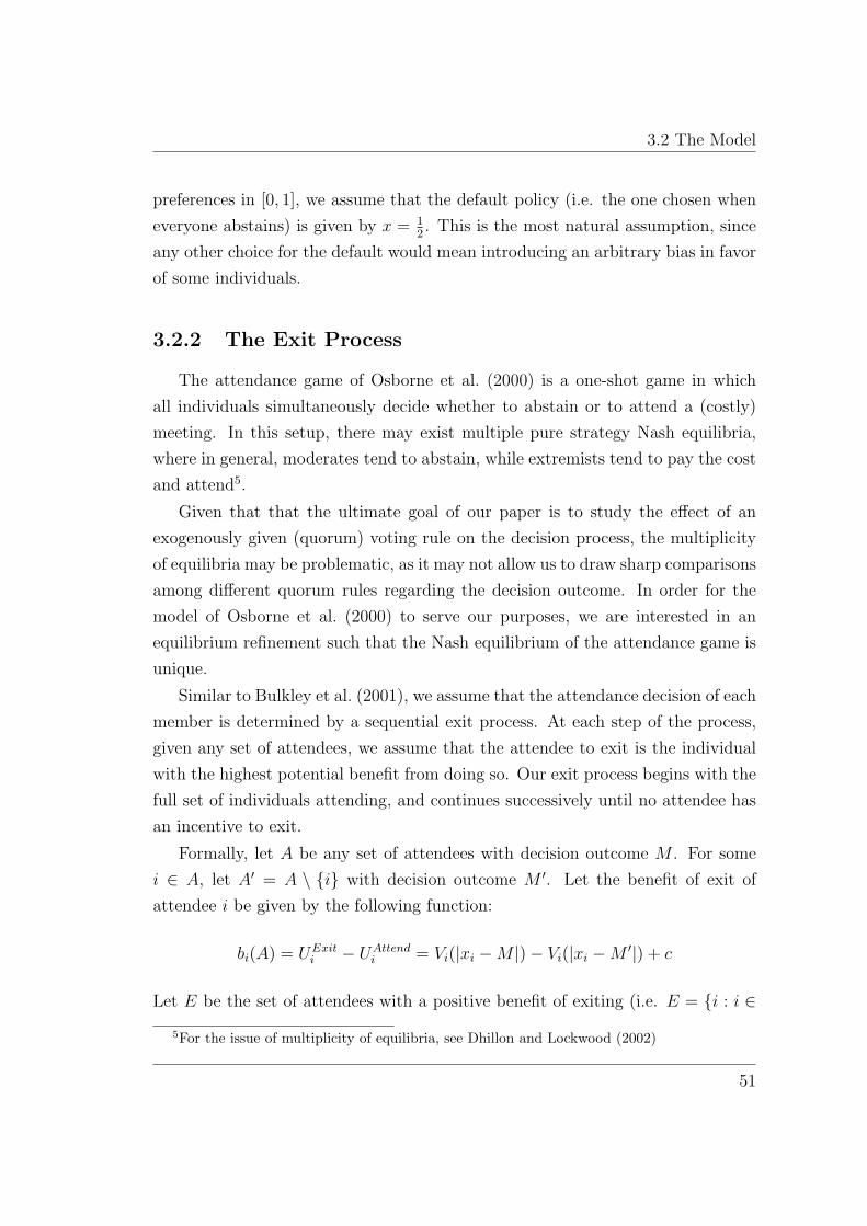
3.2 The Model
preferences in [0; 1], we assume that the default policy (i.e. the one chosen when
everyone abstains) is given by x = 12. This is the most natural assumption, since
any other choice for the default would mean introducing an arbitrary bias in favor
of some individuals.
3.2.2 The Exit Process
The attendance game of Osborne et al. (2000) is a one-shot game in which
all individuals simultaneously decide whether to abstain or to attend a (costly)
meeting. In this setup, there may exist multiple pure strategy Nash equilibria,
where in general, moderates tend to abstain, while extremists tend to pay the cost
and attend5.
Given that that the ultimate goal of our paper is to study the e�ect of an
exogenously given (quorum) voting rule on the decision process, the multiplicity
of equilibria may be problematic, as it may not allow us to draw sharp comparisons
among di�erent quorum rules regarding the decision outcome. In order for the
model of Osborne et al. (2000) to serve our purposes, we are interested in an
equilibrium re�nement such that the Nash equilibrium of the attendance game is
unique.
Similar to Bulkley et al. (2001), we assume that the attendance decision of each
member is determined by a sequential exit process. At each step of the process,
given any set of attendees, we assume that the attendee to exit is the individual
with the highest potential bene�t from doing so. Our exit process begins with the
full set of individuals attending, and continues successively until no attendee has
an incentive to exit.
Formally, let A be any set of attendees with decision outcome M . For some
i 2 A, let A0 = A n fig with decision outcome M 0. Let the bene�t of exit of
attendee i be given by the following function:
bi(A) = UExiti � UAttend
i = Vi(jxi �M j)� Vi(jxi �M 0j) + c
Let E be the set of attendees with a positive bene�t of exiting (i.e. E = fi : i 2
5For the issue of multiplicity of equilibria, see Dhillon and Lockwood (2002)
51

Participation Quorums in Costly Meetings
A and bi(A) > 0g). The exit process is de�ned as follows:
The process starts with the full set of individuals attending (i.e. A = f1; 2; :::; Ng)and proceeds in the following way:
For any committee A:
1. If E = ; then the process terminates;
2. If E 6= ; then attendee j exits, where j is de�ned by: bj(A) be the maximal
element of fbi(A)g; i 2 E;
3. If there are more than one maximal elements in E, then the attendee who
exits is drawn randomly among the ones having the maximal bi(A).
Intuitively, as in Osborne et al. (2000), when an attendee decides to exit, he
does not have to pay the cost of attending (i.e. c), while he su�ers some disutility
in terms of the decision outcome since as a result of exiting, the decision moves
further from his ideal policy (i.e. Vi(jxi�M j)�Vi(jxi�M 0j)) < 0). Notice that at
each step of the exit process, several attendees may have a positive bene�t from
exiting. Having assumed that at each step the attendee to exit is the one who has
the highest bene�t from doing so, and given that all individuals have to pay the
same cost in case of attending, the individual that actually exits is the attendee
with the smallest disutility from doing so in terms of the policy outcome (i.e. the
attendee with the lowest Vi(jxi �M 0j)� Vi(jxi �M j))).One can think of the above situation as following: Suppose that the committee
members meet in a room where the meeting has to take place. Once in the room,
the individuals have to decide whether to leave the room or to stay and pay the
(opportunity) cost of attending the meeting, and thus in uence to some extent
the decision taken. Given such a situation, and for a given cost, we assume that
the �rst individual to leave the room is the one for whom the bene�t of leaving is
the highest. After the �rst individual has left, the next member to exit (if any)
is the one with the highest bene�t from leaving given the remaining set of people
in the room, and so on.
52

3.2 The Model
A
A
A
1
2
3
A
A
A
4
5
6
A'
A'
A'
4
5
6
1 2 3 4 5
1 2 3 4 5 1 2 3 4 5X =1X =1/2X =01 3 5
X =1X =1/2X =01 3 5 X =1X =1/2X =01 3 5
d = 1N-1 = 0,25 d M
M
M
M
M
M M
M
M
l
l
l
l l
r
r
r
r r
Figure 3.1: An Example of a 5 members committee. We denote by x a member whoabstains, and with a circle a member who attends.
Example 1. In order to illustrate how a decision is reached given the exit process
defined above, suppose N = 5, so that we start with a (full) set of 5 attendees as in
situation A1. Let M denote the chosen policy for any given set of attendees, and
let M 0 denote the new chosen policy resulting from the exit of some attendee from
the committee. Then, for any given set of attendees, let m denote the attendee
located at M (when the number of attendees is odd), and let l and r denote the
first attendees on the left and on the right of M respectively.
Consider situation A1 in the figure. In that situation, we have that M = 12, which
coincides with the location of m = 3, while l = 2 and r = 4. If m exits the commit-
tee, the policy remains at 12, that is, M = M 0, so that m is willing to exit whenever
Vm(0) > Vm(0)� c, or, equivalently, c > 0. If any i 6= m exits, he would suffer a
strictly positive loss in terms of distance (i.e. Vi(jxi�M j)�Vi(jxi�M 0j) < 0 for
all i 6= m). Hence, m is the first attendee to leave (i.e. b3(A) is the max element
of E), so that we go to situation A2.
At A2, observe that both l and r are willing to leave if and only if V (14) >
V (12) � c, or, equivalently, c > V (1
2) � V (1
4). If this inequality is not satisfied,
the exit process stops here, and we are at an equilibrium (with the corresponding
policy being M = 12). Suppose now, on the contrary, that the inequality is satisfied
53

Participation Quorums in Costly Meetings
so that l and r want to leave. Notice then that at this stage, both attendees 1
and 5 might also want to exit. However, their disutility in terms of distance from
doing so is given by V (34) � V (1
2) > V (1
2) � V (1
4) by the strict convexity of V (:).
Therefore, the disutility from leaving is strictly higher for l and r than it is for 1
and 5, so that either one of the formers leaves first. Suppose, WLOG, that l exits,
so that we go to A3.
At A3, it is clear that m = 4 would exit before r = 5. Indeed, m wants to exit
if and only if c > V (14), which is true since we have assumed at stage A2 that c >
V (12)�V (1
4) and V(.) is strictly convex. Hence, m wants to leave. Then, observe
that the potential disutility of r from exiting is given by V (58)� V (1
4) > V (1
4), so
that m exits before r. Now, attendee l wants to exit if and only if c > V (78)�V (3
4).
As we cannot compare the potential disutility from exiting between m and l, either
of the two might leave first.
Suppose that V (:) is such that m exits before l, so that we are at stage A04.
Again, observe that both l = 1 and r = 5 have the same incentives to leave the
committee, that is, they want to exit if and only if c > V (1) � V (12). If this in-
equality is not satisfied, the exit process stops here, and we are at an equilibrium.
Indeed, neither l nor r want to exit, and none of the abstainers want to attend:
it is direct that neither 4 nor 2 (by symmetry) want to attend, as they just left.
Then, it is also direct that abstainer 3 has no incentive to attend, as there would be
no effect on the policy (which is already located at his ideal point) while he would
have to bear the cost of attending. Hence, as no individual wants to deviate, we
are at an equilibrium (with the corresponding policy being M = 12). Suppose now,
on the contrary, that c > V (1)�V (12), and suppose, WLOG, that l leaves, so that
we reach A05.
At A05, only attendee m is left, and the chosen policy M is at his ideal point. As
c > V (12), m leaves, and we reach A06, at which no attendee is left. As no abstainer
wants to attend, we are at an equilibrium. Indeed, it is direct that neither 5 nor
1 (by symmetry) want to attend, as they just left. Then, it follows directly that
neither 2 nor 4 want to attend either, as their potential benefit from doing so is
54
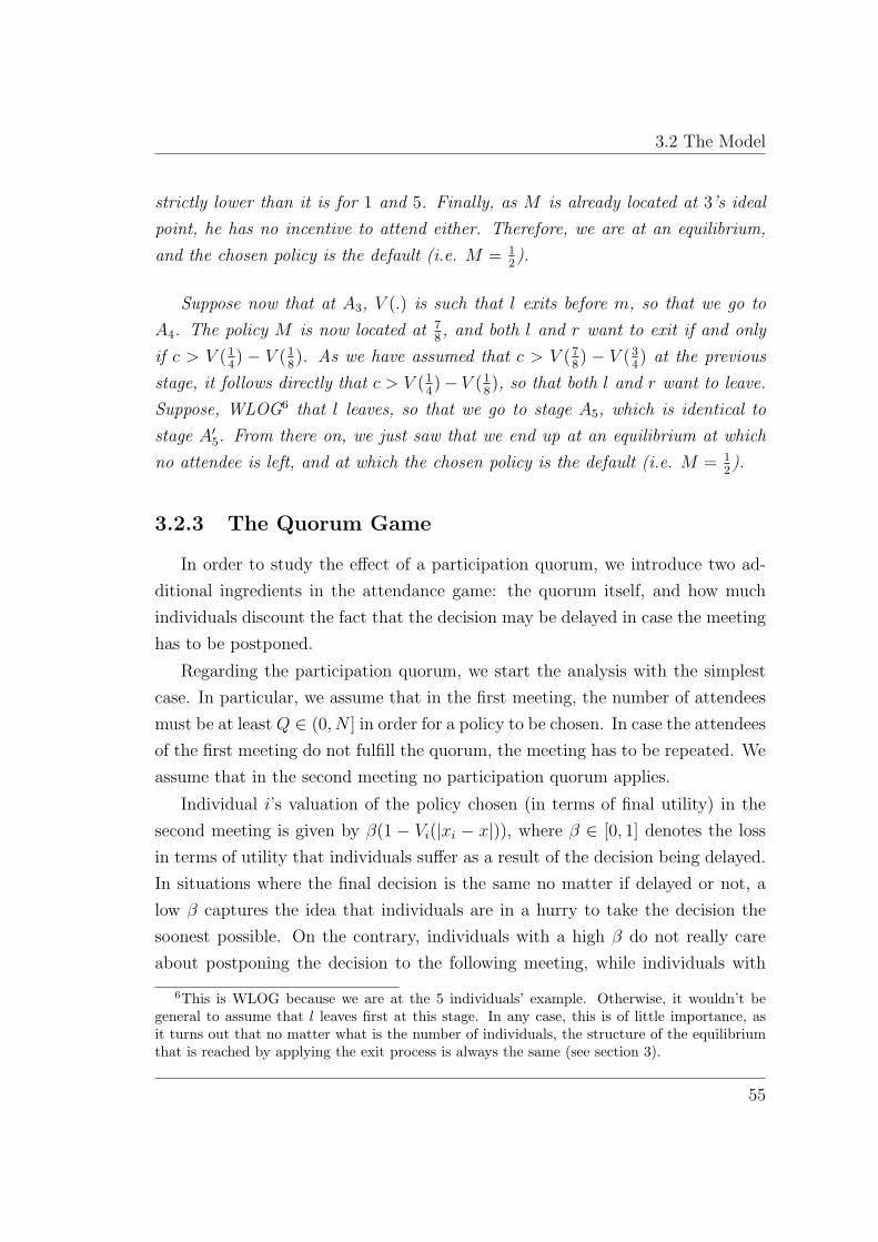
3.2 The Model
strictly lower than it is for 1 and 5. Finally, as M is already located at 3’s ideal
point, he has no incentive to attend either. Therefore, we are at an equilibrium,
and the chosen policy is the default (i.e. M = 12).
Suppose now that at A3, V (:) is such that l exits before m, so that we go to
A4. The policy M is now located at 78, and both l and r want to exit if and only
if c > V (14) � V (1
8). As we have assumed that c > V (7
8) � V (3
4) at the previous
stage, it follows directly that c > V (14)� V (1
8), so that both l and r want to leave.
Suppose, WLOG6 that l leaves, so that we go to stage A5, which is identical to
stage A05. From there on, we just saw that we end up at an equilibrium at which
no attendee is left, and at which the chosen policy is the default (i.e. M = 12).
3.2.3 The Quorum Game
In order to study the e�ect of a participation quorum, we introduce two ad-
ditional ingredients in the attendance game: the quorum itself, and how much
individuals discount the fact that the decision may be delayed in case the meeting
has to be postponed.
Regarding the participation quorum, we start the analysis with the simplest
case. In particular, we assume that in the �rst meeting, the number of attendees
must be at least Q 2 (0; N ] in order for a policy to be chosen. In case the attendees
of the �rst meeting do not ful�ll the quorum, the meeting has to be repeated. We
assume that in the second meeting no participation quorum applies.
Individual i's valuation of the policy chosen (in terms of �nal utility) in the
second meeting is given by �(1 � Vi(jxi � xj)), where � 2 [0; 1] denotes the loss
in terms of utility that individuals su�er as a result of the decision being delayed.
In situations where the �nal decision is the same no matter if delayed or not, a
low � captures the idea that individuals are in a hurry to take the decision the
soonest possible. On the contrary, individuals with a high � do not really care
about postponing the decision to the following meeting, while individuals with
6This is WLOG because we are at the 5 individuals’ example. Otherwise, it wouldn’t begeneral to assume that l leaves first at this stage. In any case, this is of little importance, asit turns out that no matter what is the number of individuals, the structure of the equilibriumthat is reached by applying the exit process is always the same (see section 3).
55

Participation Quorums in Costly Meetings
� = 1 are indi�erent whether the decision is taken in the �rst or in the second
meeting.
� Stage 1 (1st Meeting): Following the exit process de�ned above, individuals
decide whether to attend the meeting or not. If the number of attendees
is larger than Q, then a policy x is decided according to the compromise
function (here the median). Each individual gets �nal utility U1i = 1 �Vi(jxi � xj)� c�i. If the quorum is not met, the game goes to stage two.
� Stage 2 (2nd Meeting): Following the exit process de�ned above, indi-
viduals decide whether to attend the meeting or not. No matter what is
the number of participants this time, a policy x is to be chosen accord-
ing to the same compromise function. Each individual gets �nal utility
U2i = �(1� Vi(jxi � xj))� c�i.
3.3 Results
3.3.1 The Benchmark: The No-Quorum Game
In this section, we present the results for a one-shot attendance game for which
no quorum applies. Naturally, these results are similar to the ones described in
Osborne et al. (2000). To be more precise, our results characterize a unique
equilibrium that belongs to the set of equilibria of the original work by Osborne
et al. (2000). The novelty of our results lies in the fact that the equilibrium we
obtain is unique, thanks to the equilibrium re�nement through the de�ned exit
process we based on Bulkley et al. (2001).
Given the exit process we have de�ned previously, the following lemmas apply
for the equilibrium:
Lemma 1. The equilibrium number of attendees is even.
56
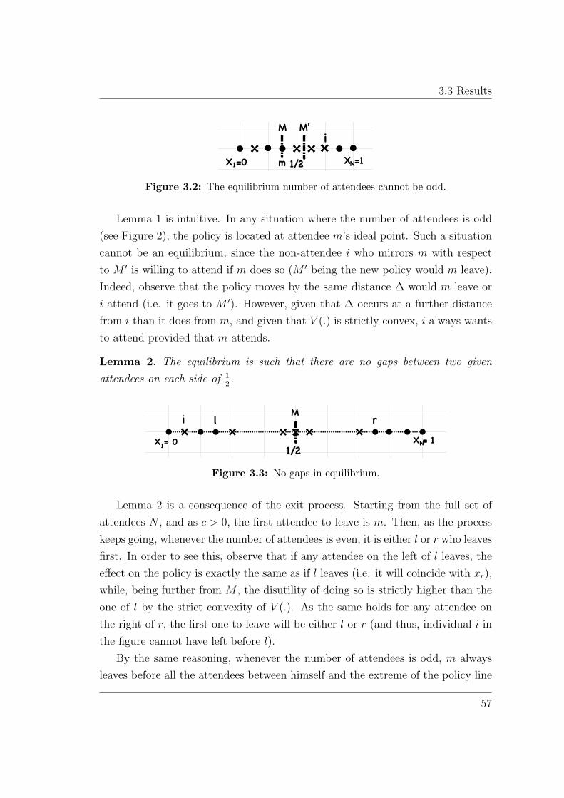
3.3 Results
N1 1/2 X =1L
X =0LK
Ml r
R
i j
i 1/2X =0 X =1
M M'
1 N
yx
m
Figure 3.2: The equilibrium number of attendees cannot be odd.
Lemma 1 is intuitive. In any situation where the number of attendees is odd
(see Figure 2), the policy is located at attendee m's ideal point. Such a situation
cannot be an equilibrium, since the non-attendee i who mirrors m with respect
to M 0 is willing to attend if m does so (M 0 being the new policy would m leave).
Indeed, observe that the policy moves by the same distance � would m leave or
i attend (i.e. it goes to M 0). However, given that � occurs at a further distance
from i than it does from m, and given that V (:) is strictly convex, i always wants
to attend provided that m attends.
Lemma 2. The equilibrium is such that there are no gaps between two given
attendees on each side of 12.
X = 01
M
X = 1N1/2
X = 01
M
X = 1N1/2
tkd t2 2
X = 01
M
X = 1N1/2
tkd t2 2
l
l
l ri
Figure 3.3: No gaps in equilibrium.
Lemma 2 is a consequence of the exit process. Starting from the full set of
attendees N , and as c > 0, the �rst attendee to leave is m. Then, as the process
keeps going, whenever the number of attendees is even, it is either l or r who leaves
�rst. In order to see this, observe that if any attendee on the left of l leaves, the
e�ect on the policy is exactly the same as if l leaves (i.e. it will coincide with xr),
while, being further from M , the disutility of doing so is strictly higher than the
one of l by the strict convexity of V (:). As the same holds for any attendee on
the right of r, the �rst one to leave will be either l or r (and thus, individual i in
the �gure cannot have left before l).
By the same reasoning, whenever the number of attendees is odd, m always
leaves before all the attendees between himself and the extreme of the policy line
57

Participation Quorums in Costly Meetings
(i.e. 0 or 1), while the same holds for the �rst attendee on the other side on 1=2
(i.e. l or r). Therefore, it is always either m, or r, or l leaving �rst, and there can
be no gaps between any two attendees on each side of 1=2 in equilibrium.
Corollary 1. If there are attendees on both sides of 1=2, the individuals located
at 0 and 1 attend.
At any stage of the exit process such that there are attendees on both sides of
1=2, the attendee located at 0 (respectively 1) has strictly higher disutility from
leaving than l (respectively r). Hence, it follows directly that any such stage, both
the individuals at 0 and 1 attend.
Lemma 3. The equilibrium is balanced. That is, the number of attendees on each
side of 12
is the same.
N1 1/2 X =1L
X =0LK
Ml r
R
i j
i 1/2X =0 X =1
M M'
1 N
yx
m
Figure 3.4: The equilibrium number of attendees can not be unbalanced.
Given that at an equilibrium, the number of attendees is even (Lemma 1), and
that there can be no gaps between any two attendees on each side of 12
(Lemma
2), then a situation in which the number of attendees is unbalanced is such that
the number of attendees between 0 and 1=2 is strictly smaller (or higher) than the
number of attendees between 1=2 and 1. Such a situation, as depicted in Figure
4, cannot be an equilibrium since if l and r are attending, any given abstainer is
also willing to attend provided that V (:) is strictly convex.
We are now ready to characterize the (unique) equilibrium of the attendance
game given the exit process:
Proposition 1. For any c > 0, let t be the unique solution of c = V (2t)� V (t).
If t > 12, then for all N > 2, A� = 0. If t < 1
2, then, for all N > 2, there exists
a unique equilibrium at which any individual i with xi 2[0; 1
2� t) [ (1
2+ t; 1
]attends. The equilibrium number of attendees is given by A� = 2(k + 1), where
k 2 N is the maximum natural number such that k < (12� t)(N � 1).
58
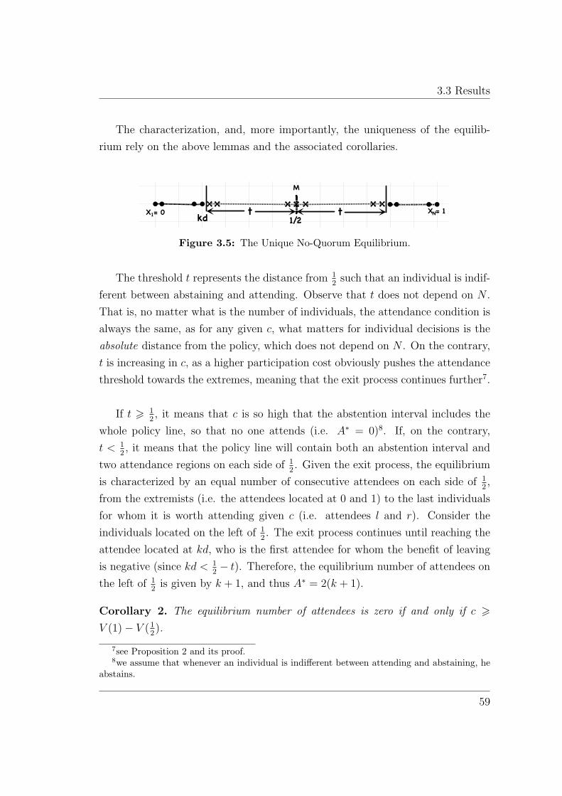
3.3 Results
The characterization, and, more importantly, the uniqueness of the equilib-
rium rely on the above lemmas and the associated corollaries.
X = 01
M
X = 1N1/2
tkd t
Figure 3.5: The Unique No-Quorum Equilibrium.
The threshold t represents the distance from 12
such that an individual is indif-
ferent between abstaining and attending. Observe that t does not depend on N .
That is, no matter what is the number of individuals, the attendance condition is
always the same, as for any given c, what matters for individual decisions is the
absolute distance from the policy, which does not depend on N . On the contrary,
t is increasing in c, as a higher participation cost obviously pushes the attendance
threshold towards the extremes, meaning that the exit process continues further7.
If t > 12, it means that c is so high that the abstention interval includes the
whole policy line, so that no one attends (i.e. A� = 0)8. If, on the contrary,
t < 12, it means that the policy line will contain both an abstention interval and
two attendance regions on each side of 12. Given the exit process, the equilibrium
is characterized by an equal number of consecutive attendees on each side of 12,
from the extremists (i.e. the attendees located at 0 and 1) to the last individuals
for whom it is worth attending given c (i.e. attendees l and r). Consider the
individuals located on the left of 12. The exit process continues until reaching the
attendee located at kd, who is the �rst attendee for whom the bene�t of leaving
is negative (since kd < 12� t). Therefore, the equilibrium number of attendees on
the left of 12
is given by k + 1, and thus A� = 2(k + 1).
Corollary 2. The equilibrium number of attendees is zero if and only if c >
V (1)� V (12).
7see Proposition 2 and its proof.8we assume that whenever an individual is indifferent between attending and abstaining, he
abstains.
59

Participation Quorums in Costly Meetings
From the above corollary, there exists a threshold value of c (which corresponds
to t = 1=2) such that no individual wants to attend the meeting. As it was the
case for t, observe that the threshold value of c is constant. In particular, it does
not depend on the number of individuals N .
Corollary 3. The equilibrium policy x� is always 12.
Given the symmetric structure of the equilibrium, it turns out that the equi-
librium policy is always located at the middle of the policy line (i.e. at 12) no
matter what is the number of attendees.
Finally, Proposition 2 below gives some comparative statics results regarding
the participation cost c and the number of individuals N on the equilibrium
number of attendees.
Proposition 2. The equilibrium number of attendees is decreasing in the atten-
dance cost. Furthermore, both the number of attendees and abstainers is nonde-
creasing in the number of individuals.
The comparative statics results in the above proposition are intuitive. For
given N , an increase in the attendance cost c implies that the exit process con-
tinues further. That is, the most moderate attendees from the original set of
attendees might not �nd it worthwhile any longer to attend, given that the cost
of participation has increased. Therefore, the equilibrium number of attendees
decreases. Moreover, given that an increase in the number of individuals N does
not alter the indi�erence threshold on the policy line between attending and ab-
staining, it follows that such an increase directly translates into a higher (or at
least equal) equilibrium number of both attendees and abstainers.
3.3.2 The Quorum Game
Having characterized the unique equilibrium of the No-Quorum Game, we
can apply the results to the analysis of the Quorum Game. Remember that the
Quorum Game consists of two meetings. In the second meeting there is no quorum
requirement, while in the �rst one, a participation quorum Q 2 (0; N ] has to be
ful�lled in order for a decision to be taken.
60

3.3 Results
Notation 1. We use subindexes 1 and 2 to refer to the first and second round of
the quorum game, while no subindex refers to the one-shot no-quorum game.
We begin the analysis of the quorum game with the second meeting, if this
were to be required.
Lemma 4 (Second Meeting). For any c > 0, let t2 be the unique solution of
c = �[V (2t2) � V (t2)]. If t2 > 12, then for all N > 2, A�2 = 0. If t2 < 1
2,
then, for all N > 2, there exists a unique equilibrium at which any individual i
with xi 2[0; 1
2� t2) [ (1
2+ t2; 1
]attends. The equilibrium number of attendees is
given by A�2 = 2(k2 + 1), where k2 2 N is the maximum natural number such that
k2 < (12� t2)(N � 1).
Lemma 4 has exactly the same avor as Proposition 1. The equilibrium has a
very similar structure, the chosen policy at the second stage is x�2 = 1=2, and the
only (but important) di�erence is that the number of attendees may decrease.
Proposition 3. A�2 6 A�
The number of attendees in the second meeting, if a�ected, is lower than that
of the no-quorum game. Remember that in the second meeting, each individual
discounts the decision taken (i.e. � 2 [0; 1]). More speci�cally, the e�ect of
one's attendance in terms of �nal utility is discounted, and hence some moderates
that would have incentives to attend the one-shot no-quorum meeting may not
participate in the second one. This is the case if their incentives to attend in
terms of their (small) in uence on the postponed decision do not compensate the
cost of attending.
In order to characterize the equilibrium of the quorum game, the following
de�nitions will be helpful. Thereafter we present the main contribution of our
analysis in Proposition 4.
Definition 1. Let the threshold values of the discount factor be defined as follows:
�1 = 1� c1�V (jkd� 1
2j) ; �2 = c
V (j1�2kdj)�V (jkd� 12j) ; �3 = 1� c
1�V (j(Q2�1)d� 1
2j);
�4 = 1�c1�V (j(Q−1
2)d� 1
2j); �5 =
1�V (j1�(Q−12
)dj)1�V ( 1
2)
61

Participation Quorums in Costly Meetings
Proposition 4. For any c > 0, N > 2 and Q 2 (0; N ] there exists a unique
equilibrium that is characterized as follows:
Table 3.1: Equilibrium of the Quorum Game
Q Q < A� Q = A� Q > A�
Q even Q odd
� � 2 [0; 1] � 2 (�1; �2] otherwise � < �3 otherwise � < minf�4; �5g otherwise
A�1 A� 0 Q Q 0 Q 0
A�2 { 2(k2 + 1) { { 2(k2 + 1) { 2(k2 + 1)
x� 1=2 1=2 1=2 1=2 1=2 (Q�12
)d 1=2
According to the above proposition, the e�ect of the quorum on the equilibrium
(i.e. A�1; A�2 and x�) depends on the level of the quorum itself (i.e. Q), and on
how much individuals discount a delayed decision (i.e. �). To be more precise,
the only case for which the equilibrium outcome is independent of � (and the
decision always taken in the �rst meeting), is when the quorum is lower than the
no-quorum attendance rate (i.e. Q < A�). On the contrary, when Q > A�, how
much individuals discount a delayed decision is crucial.
1. Q < A�: If the quorum is smaller than the no-quorum attendance rate,
then it has no e�ect on the equilibrium outcome. This is a consequence of the fact
that the quorum does not alter the exit decision of any of the individuals during
the �rst meeting and hence the policy decision remains una�ected.
2. Q = A�: When the quorum is equal to the number of attendees in the
no-quorum game, we know that A� and hence the quorum is even. Moreover, we
know that individual l located at kd is the �rst attendee who decided not to exit
the no-quorum game (see Figure 6)9.
9WLOG we analyze the decision of individual l, while the same holds for individual r.
62
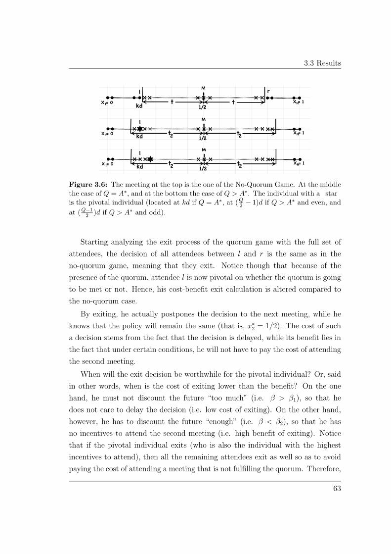
3.3 Results
X = 01
M
X = 1N1/2
tkd t
X = 01
M
X = 1N1/2
tkd t2 2
X = 01
M
X = 1N1/2
tkd t2 2
l
l r
l
Figure 3.6: The meeting at the top is the one of the No-Quorum Game. At the middlethe case of Q = A∗, and at the bottom the case of Q > A∗. The individual with a � star�is the pivotal individual (located at kd if Q = A∗, at (Q2 − 1)d if Q > A∗and even, andat (Q−1
2 )d if Q > A∗and odd).
Starting analyzing the exit process of the quorum game with the full set of
attendees, the decision of all attendees between l and r is the same as in the
no-quorum game, meaning that they exit. Notice though that because of the
presence of the quorum, attendee l is now pivotal on whether the quorum is going
to be met or not. Hence, his cost-benefit exit calculation is altered compared to
the no-quorum case.
By exiting, he actually postpones the decision to the next meeting, while he
knows that the policy will remain the same (that is, x∗2 = 1/2). The cost of such
a decision stems from the fact that the decision is delayed, while its benefit lies in
the fact that under certain conditions, he will not have to pay the cost of attending
the second meeting.
When will the exit decision be worthwhile for the pivotal individual? Or, said
in other words, when is the cost of exiting lower than the benefit? On the one
hand, he must not discount the future “ too much” (i.e. β > β1), so that he
does not care to delay the decision (i.e. low cost of exiting). On the other hand,
however, he has to discount the future “ enough” (i.e. β < β2), so that he has
no incentives to attend the second meeting (i.e. high benefit of exiting). Notice
that if the pivotal individual exits (who is also the individual with the highest
incentives to attend), then all the remaining attendees exit as well so as to avoid
paying the cost of attending a meeting that is not fulfilling the quorum. Therefore,
63
Participation Quorums in Costly Meetings
if � 2 (�1; �2), then A�1 = 0; A�2 = 2(k2 + 1) and x� = 1=2.
If the above restriction on the discount factor does not hold (i.e. � =2 (�1; �2)),
for example because the pivotal individual discounts the future a lot, then the
quorum equilibrium is identical to the no-quorum one and the quorum is binding
in the �rst round.
3. Q > A�: If the quorum is larger than the number of attendees in the
no-quorum game, its e�ect on the equilibrium varies depending on whether the
quorum is even or odd.
(a) Q Even: The intuition in this case is similar to the one where Q = A�.
However, an important di�erence is that when Q > A�, the pivotal individual is
now located at (Q2� 1)d, and hence is more moderate than the pivotal individual
at Q = A�10.
During the exit process of the quorum game, the pivotal attendee is the �rst
individual whose exit decision may be altered because of the presence of the
quorum. By exiting, he actually postpones the decision to the next meeting,
being sure that the policy will remain the same (that is x�2 = 1=2). Moreover, and
contrary to the Q = A� case, he de�nitely has no incentives to attend the second
meeting, given that he is an abstainer in the no-quorum game.
The bene�t of attending stems from the fact that the decision is not delayed,
while it implies an extra attendance cost. Hence, the pivotal individual is willing
to pay the cost, attend and make the quorum binding in the �rst meeting if he
discounts a lot a delayed decision (i.e. � < �3). On the contrary, if � > �3, the
pivotal individual has no incentives to pay the cost, the quorum is not met and as
before no one attends the �rst meeting (i.e. A�1 = 0; A�2 = 2(k2 +1) and x� = 1=2).
(b) Q Odd: The intuition in this case is similar but with a very important
di�erence with respect to the case of an even quorum. The pivotal individual
is located at (Q�12
)d, who is again more moderate than the pivotal individual at
Q = A�11.
Through the exit process of the quorum game, the pivotal attendee is the
�rst individual whose exit decision may be altered because of the presence of
10WLOG we analyze the individual located at (Q2 � 1)d. Because of symmetry, the same
analysis holds for his mirror with respect to 1/2.11For the same reasoning as Footnote 7, WLOG we analyze the individual located at (Q−1
2 )d.
64

3.3 Results
the quorum. By exiting, he actually postpones the decision to the next meeting,
being sure that the policy will remain the same (that is x�2 = 1=2). As before,
he de�nitely has no incentives to attend the second meeting, given that he is an
abstainer in the no-quorum game.
The bene�t of attending has now an additional component compared to the
case of an even quorum. In addition to not being delayed, the elected policy moves
to his ideal point (since the pivotal attendee is the new median). As before, the
cost is what the individual has to pay in order to attend the meeting. Hence,
the pivotal individual is willing to pay the cost, attend and make the quorum
binding in the �rst meeting if he discounts a lot a delayed decision (i.e. � < �4).
On the contrary, if � > �4, the pivotal individual has no incentives to pay the
cost, the quorum is not met and as before no one attends the �rst meeting (i.e.
A�1 = 0; A�2 = 2(k2 + 1) and x� = 1=2).
Notice though that the attendance of the pivotal member implies a policy
distortion. Indeed, the policy now moves to x� = Q�12d 6 1
2, and given that the
exit process is altered, it deserves a closer look. In order to guarantee that the
exit process terminates at an equilibrium, we have to make sure that no further
attendees have incentives to exit, while no further abstainers want to attend.
The process actually terminates if the attendee with the highest bene�t of
exiting is not willing to do so. Notice that the policy is biased towards the left
(i.e. x� = Q�12d 6 1
2). Moreover, any attendee that exits guarantees a delayed
policy outcome of 1=2. The individual with the highest incentives to do so is then
the extremist located the furthest from x� = Q�12d, that is, the individual located
at 1. In order for this extremist not to exit, it has to be the case that he is harmed
a lot by postponing the decision to the second meeting (i.e. � < �5).
The individual with the highest bene�t of entering is the mirror (with respect
to 1=2) of the individual located at x�. Observe that this individual is never
attending a no-quorum meeting, precisely because it is not worthwhile for him
to pay the cost so as to push the policy from x� to 1=2. Therefore, he has no
incentives to attend here either. Notice that in fact, this individual free rides
on the attendance of his `mirror" who participates so as to avoid postponing the
decision.
65

Participation Quorums in Costly Meetings
To sum up, our results regarding the Quorum Game can be summarized as
following:
� The quorum is met in the �rst round when:
1. The quorum is lower than the no-quorum attendance rate.
2. The quorum is higher than the no-quorum attendance rate and mem-
bers discount a lot a delayed decision.
� If the second meeting takes place, the number of attendees is smaller or
equal than in the no-quorum case.
� When the quorum is larger or equal than the no-quorum attendance rate,
then either no member attends the �rst meeting or the quorum is binding.
Notice that there exists no equilibrium in which a subset of members decide
to attend the �rst meeting and the quorum is not met12.
� The quorum has a di�erent e�ect when it is even or odd. An odd quorum
may create policy distortions.
Regarding the e�ect of the quorum on total welfare welfare, we conclude that
the introduction of quorum requirement is welfare decreasing. Whenever the
quorum has no e�ect on the equilibrium, that is, when the decision is taken in
the �rst meeting and both the number of attendees and the equilibrium policy
remain the same, total welfare is clearly not a�ected.
Whenever the quorum is binding, but the equilibrium policy unchanged, total
welfare is strictly lower than under the no-quorum equilibrium. Indeed, as the
presence of the quorum \forces" some moderates to attend (and thus bear the
corresponding cost) in order for the meeting not to be postponed, total welfare
is strictly lower following the introduction of the quorum. If, in addition to that,
the equilibrium policy gets distorted (i.e. x� 6= 12), the e�ect of the quorum is
even worse from a welfare perspective.
12A possible way to obtain such a result would be to introduce an exogenous probability thateach individual may be prevented from attending the meeting.
66

3.4 Conclusion
Finally, although not formally proven, through simulations we conclude that
when the decision is postponed to the second meeting, and even though less in-
dividuals attend, total welfare is lowered as a result of the quorum being present.
That is, the fact that less individuals pay the cost of attending does not compen-
sate the aggregate loss of welfare in terms of policy valuation.
3.4 Conclusion
We believe that this piece of research is a �rst step towards the understanding
of a widely used but not formally analyzed voting rule. Clearly, our results have
important policy implications, and we think that policy makers deciding on the
use of a participation quorum in small decision making meetings should take our
results into consideration.
In particular, in meetings where the preferences of individuals are symmetri-
cally distributed, introducing a participation quorum is a bad idea since it creates
welfare losses. As explained, these losses may be the result of the decision be-
ing delayed, or the consequence of the fact that individuals who are better o�
abstaining are now \forced" to attend in order to ful�ll the quorum.
One standard argument in favor of the use of a participation quorum is that it
allows to protect individuals from a policy decision being taken by a small minority
of the members. However, it turns out that the policy is in general not a�ected as
it coincides with the one that would have been taken had there been no quorum.
This is so because in a world where the the costly committee meetings are ruled
by the \citizen-candidate" spirit of Osborne et al. (2000), the individuals who are
really afraid of a unwanted decision have incentives to attend anyway. In order to
protect those individuals, there is then no need for a participation quorum since
their participation is in line with their own interest, and hence this argument does
not apply.
A �nal argument in favor of a participation quorum is that it guarantees the
legitimacy of the decision taken. Think for instance of a meeting of the share-
holders of an important enterprise deciding on the enterprise's strategy. Suppose
that all shareholders have a very high opportunity cost of attending the meeting,
67
Participation Quorums in Costly Meetings
so that the equilibrium number of attendees under no quorum is very small. In
such cases, one can think of a participation quorum as a tool to protect the legiti-
macy of the decision, since a decision taken by very few shareholders might have a
rather negative impact on the enterprise's image. According to our results, if the
shareholders are in a hurry, introducing a quorum then has the e�ect of increasing
the number of shareholders who take part in the decision. In such situations, our
analysis has policy recommendations as well. We showed that the use of a partic-
ipation quorum always lowers welfare. In any case, however, if there is a quorum
to be introduced, it should require an even number of individuals so as to avoid
policy distortions (and thus minimize welfare losses).
As the present paper constitutes a �rst attempt to analyze the use of a partic-
ipation quorum in meetings, many paths for future research remain open. Among
those, a very important feature which we wish to capture is the case in which a
positive number of members show up at the �rst meeting, but the quorum is not
ful�lled. A way to allow for such a possibility could be the introduction of an
exogenous probability that each member is prevented from attending the meet-
ing. Intuitively, this would a�ect the number of attendees in each meeting and,
more importantly, it would give rise to situations in which some individuals end
up paying the cost of attending (even though the meeting has to be postponed),
because they believe the quorum will be met.
So far our analysis has been focused on the case of uniformly distributed in-
dividuals' favorite positions. Although our results would still be valid for other
symmetric distributions, we believe it is important to extend our analysis to asym-
metric setups. Indeed, one of the main arguments favoring the use of a participa-
tion quorum is the fact that one wants to prevent the decision from being taken
by a (non-representative) minority. However, in symmetric situations such as the
one we have been analyzing here, there is no way a minority could possibly exploit
a majority.
68
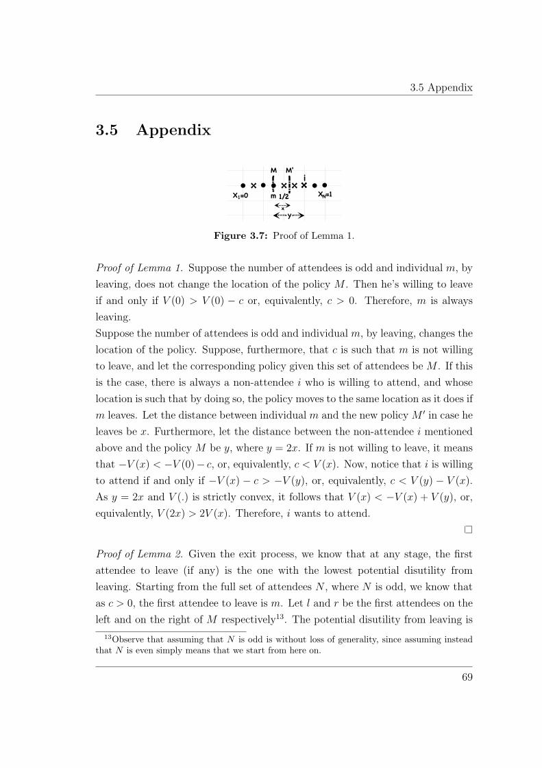
3.5 Appendix
3.5 AppendixN1 1/2 X =1
LX =0
LK
Ml r
R
i j
i 1/2X =0 X =1
M M'
1 N
yx
m
Figure 3.7: Proof of Lemma 1.
Proof of Lemma 1. Suppose the number of attendees is odd and individual m, by
leaving, does not change the location of the policy M . Then he's willing to leave
if and only if V (0) > V (0) � c or, equivalently, c > 0. Therefore, m is always
leaving.
Suppose the number of attendees is odd and individual m, by leaving, changes the
location of the policy. Suppose, furthermore, that c is such that m is not willing
to leave, and let the corresponding policy given this set of attendees be M . If this
is the case, there is always a non-attendee i who is willing to attend, and whose
location is such that by doing so, the policy moves to the same location as it does if
m leaves. Let the distance between individual m and the new policy M 0 in case he
leaves be x. Furthermore, let the distance between the non-attendee i mentioned
above and the policy M be y, where y = 2x. If m is not willing to leave, it means
that �V (x) < �V (0)� c, or, equivalently, c < V (x). Now, notice that i is willing
to attend if and only if �V (x) � c > �V (y), or, equivalently, c < V (y) � V (x).
As y = 2x and V (:) is strictly convex, it follows that V (x) < �V (x) + V (y), or,
equivalently, V (2x) > 2V (x). Therefore, i wants to attend.
Proof of Lemma 2. Given the exit process, we know that at any stage, the �rst
attendee to leave (if any) is the one with the lowest potential disutility from
leaving. Starting from the full set of attendees N , where N is odd, we know that
as c > 0, the �rst attendee to leave is m. Let l and r be the �rst attendees on the
left and on the right of M respectively13. The potential disutility from leaving is
13Observe that assuming that N is odd is without loss of generality, since assuming insteadthat N is even simply means that we start from here on.
69

Participation Quorums in Costly Meetings
the same for both of them, and is given by V (2d)� V (d). Consider now the next
attendees on the left of l and on the right of r respectively. Their disutility from
leaving is identical, and is given by V (3d) � V (2d), which is strictly higher than
V (2d)� V (d) given the strict convexity of V (:). Obviously, this will also be true
for any pair of attendees who are located even further from M . Therefore, the
�rst one to leave is either l or r. From there on, if c is high enough so that the
exit process keeps going,
1. At any stage for which the number of attendees is odd (case A3 in Example
1), either m, or one (and only one) of the attendees l or r is the �rst one to
leave. Given the exit process, a situation in which the number of attendees
is odd is such that m is next to r (l), while, as some attendees have already
left, there are gaps between m and l (r). Suppose, WLOG, that m is next to
r (as in case A3) and let kd be the distance between m and l (so that k = 3
in the example). We aim at showing that the �rst one to leave is either m
or l (that is, either the median attendee or the furthest one next to him). If
m leaves, his disutility from doing so is given by V ( (k�1)d2
). If r leaves, he
will su�er a disutility of V (kd2
+ d)� V (d). As V ( (k�1)d2
) = V ( (k+1)d2� d) <
V ( (k+1)d2
) � V (d), it follows that m always leaves before r. Obviously, this
is also true for any attendee on the right of r. Indeed, if any such attendee
leaves, the e�ect on the policy will be exactly the same as if r leaves, while,
being strictly further, the disutility from leaving in terms of distance will be
strictly higher than the one of r by the strict convexity of V (:).
Now, if l leaves, his disutility from doing so is given by V ((k+ 12)d)�V (kd).
We do not know whether it is m or l who has the lowest disutility from
leaving. However, by the same reasoning as the one just described above, we
know that any attendee on the left of l will su�er a strictly higher disutility
from leaving than l, so that l always leaves �rst. Therefore, either m or l
leaves �rst.
2. At any stage for which the number of attendees is even (cases A4 and A04
in Example 1), so that the policy is M = (xl+xr)2
, either l or r is the �rst
one to leave. Let kd be the distance between i and M , i = l; r (so that
k = 12
in situation A4 and k = 2 in situation A04). The disutility from
70

3.5 Appendix
leaving for individual i = l, r is given by V (2kd) − V (kd). Consider now
the next attendees on the left of l and on the right of r respectively. Their
disutility from leaving is strictly higher than V (2kd)−V (kd) given the strict
convexity of V (.). Furthermore, this is also true for any pair of attendees
who are located even further from M .
Proof of Corollary 1. Consider any stage of the exit process such that there are
still attendees on both sides of 1/2 (i.e. we rule out situations such as A4 in
Example 1). From Lemma 3, we know that, no matter whether the number of
attendees is even or odd, the first one to leave is always either m, or l, or r.
Therefore, it follows directly that at any such stage (i.e. such that there are
attendees on both sides of 1/2), the attendee located at 0 (respectively 1) has
strictly higher disutility from leaving than l (respectively r). Hence, at any such
stage, both the individuals at 0 and 1 attend.
Figure 3.8: Proof of Lemma 3.
Proof of Lemma 3. Let L � 0 be the number of attendees on the left of 1/2.
Similarly, let R be the number of attendees on the right of 1/2, and assume,
WLOG, that R � L, and so R = L + K, where K > 0 and is even by Lemma 1.
From Lemma 2, it follows that the L and R attendees respectively on the left and
on the right of 1/2 are consecutive (i.e. there are no gaps between them). Let M
be the chosen policy given this set of attendees, which is located at the median
of the K attendees. Observe that if the attendees l and r are not willing to leave,
it means that c is small enough so that it is worth attending to prevent M from
moving by 12d, that is, it means that c < V (d) − V (1
2d). Let i and j be the first
attendees on the left and on the right of 1/2 respectively, and consider any non-
attendee between i and j. If any such non-attendee were to come back, the policy
71
Participation Quorums in Costly Meetings
would move to xl, and he would do so if and only if c < V ((k + 12)d) � V (kd),
where kd > d is the distance between any non-attendee and l. It turns out
that if r attends, any abstainer between i and j wants to attend as well, that is,
V ((k+ 12)d)�V (kd) > V (d)�V (1
2d) for all k > 1 by the strict convexity of V (:).
Therefore, the equilibrium is such that K = 0 (i.e. balanced).
Proof of Proposition 1. By lemmas 1 to 3 and the associated corollaries, we know
that the equilibrium reached by means of the exit process is such that there is
an equal number of attendees on each side of 12
without gaps between any two
of them, and such that the individuals located at the extremes of the policy line
attend. Let t be the unique solution of c = V (2t)� V (t) and consider a situation
such as A1 in Figure 9. By de�nition of t (and by the lemmas and associated
corollaries), any such situation, that is, any situation with an equal number of
consecutive attendees starting from the extremes on both sides of 12, and such
that only individuals with xi 2[0; 1
2� t) [ (1
2+ t; 1
]attend, is an equilibrium.
Indeed, notice that the individuals with the highest potential bene�t from leaving
are l and r. However, as by de�nition of t, bl(A) = br(A) < 0, they both attend.
Furthermore, as by de�nition of t, bi(A) > 0 for any i with xi 2[
12� t; 1
2+ t],
none of such individuals is willing to attend. Therefore, the situation depicted in
the �gure is an equilibrium.
In order to derive the equilibrium number of attendees A�, observe that the
exit process stops at the individual located at kd (i.e. attendee l), who is the �rst
attendee (on the left side of 12) for whom bi(A) < 0. Therefore, the equilibrium
number of attendees on the left of 12
is given by k + 1, and thus A� = 2(k + 1).
72

3.5 Appendix
X = 01
M
X = 1N1/2
tkd t
X = 01
M
X = 1N1/2
tkd t
l r
X = 01
M
X = 1N1/2
tkd t
A
A
A
1
3
2l
l
r
r
Figure 3.9: Proof of Proposition 1: Uniqueness
It now remains to be shown that the equilibrium is unique. Consider a situ-
ation such as A2 in the �gure. That is, a situation that satis�es the equilibrium
requirements as described in the lemmas, but such that there is one (or more)
pair(s) of consecutive attendees in the interval[
12� t; 1
2+ t]
(or, equivalently,
such that xl; xr 2[
12� t; 1
2+ t]). As, by de�nition of t, bi(A) > 0 for any i with
xi 2[
12� t; 1
2+ t], it follows that, for any t, any such situation cannot be an
equilibrium.
Finally, consider a situation such as A3 in the �gure. That is, a situation that
satis�es the equilibrium requirements as described in the lemmas, but such that
there is one (or more) pair(s) of consecutive abstainers in the interval[0; 1
2� t) [ (1
2+ t; 1
].
As, by de�nition of t, bi(A) < 0 for any i with xi 2[0; 1
2� t) [ (1
2+ t; 1
], it follows
that, for any t, any such situation cannot be an equilibrium.
Proof of Corollary 2. According to the exit process, if everybody leaves, the last
attendee to exit is either the one located at 0 or the one located at 1. This
individual is indi�erent to leave if and only if c = V (1) � V (12), or, equivalently,
t = 12. Obviously, if c > V (1) � V (1
2), or, equivalently, t > 1
2, this last attendee
wants to exit, which means that no one attends.
Proof of Proposition 2. The equilibrium value of t is implicitly de�ned by ε(t) =
73
Participation Quorums in Costly Meetings
c� V (2t) + V (t) = 0. We have that
@ε
@t= �2V 0(2t) + V 0(t) < 0
@ε
@c= 1 > 0
and thus, by the implicit function theorem: @t@c
= �∂φ∂c∂φ∂t
> 0. Therefore, as the
threshold for attendance is moving towards the extremes of the policy line as c
increases, it follows directly that the equilibrium number of attendees decreases.
Given that t does not depend on the number of individuals N , it is also direct
that the absolute number of both attendees and abstainers is increasing in N .
Indeed, for a given c > 0 and given the (�xed) distance t, increasing the (uniformly
distributed) number of individuals obviously means that there will be more (or at
least an equal number of) individuals both between 0 and t (respectively t and 1)
and in the abstention interval.
Proof of Proposition 3. As t is the unique solution of c = V (2t) � V (t) and t2 is
the unique solution of c = � [V (2t2)� V (t2)], we have that
� =V (2t)� V (t)
V (2t2)� V (t2)
As � 6 1, it follows that t2 > t, and thus k2 6 k and A�2 6 A�.
Proof of Proposition 4. 1. Suppose Q < A� and consider attendees l and r of
the no-quorum game for given N and c. Thus, bl(A�) = br(A
�) < 0, the set
E is empty and there are A� attendees in equilibrium. Let now introduce a
quorum Q < A�. All moderates located between l and r of the no-quorum
game exit, as before. Then, bl(A�1) = br(A
�1) < 0 and the set E is empty, so
that the exit process stops at l and r. Therefore, A�1 = A� and x�1 = x� = 12.
Said in words, the attendance decision of any individual is the same as in
the no-quorum case (in particular, l is not pivotal regarding the quorum
requirement), and hence the equilibrium in una�ected.
74
3.5 Appendix
2. Suppose Q = A�. All moderates located between l and r of the no-quorum
game exit, as before. Then, WLOG, given that l is now pivotal regarding
Q, he exits if and only if
1� V (jkd� 1
2j)� c < �
[1� V (jkd� 1
2j)]� �lc
where �l = 1 if and only if
� >c
V (j1� 2kdj)� V (jkd� 12j)
= �2
and �l = 0 otherwise. Suppose that � < �2, so that l would not attend in
the second round (otherwise, the second round is never reached as l has no
incentive to exit in the �rst round). Then, he exits in the �rst round if and
only if
� > 1� c
1� V (jkd� 12j)
= �1
Therefore, l exits in the �rst round if and only if �1 < � < �2. Suppose
this is the case. Notice that l is the abstainer with the highest potential
bene�t from attending so as to ful�ll Q, and thus no other abstainer has
an incentive to attend either. Given that l exits, all other attendees exit
as well since the quorum is not met and c > 0. Hence, A�1 = 0 and we go
to stage 2. From there on, the characterization of the equilibrium and its
uniqueness follow the same reasoning as in Proposition 1 (with t2 being the
unique solution of c = � [V (2t2)� V (t2)] as the new attendance threshold
and x�2 = 12).
If � < �1, l has no incentive to exit in the �rst round. The exit process
stops here, and as no individual has an incentive to deviate, we are at an
equilibrium, and it follows that A�1 = A� and x�1 = x� = 12. Similarly, if
� > �2, l would attend in the second round, so that he has no incentive to
exit in the �rst round, and the same conclusion applies.
3. Suppose Q > A� is even. Then, during the exit process, WLOG, the
attendee i located at (Q2� 1)d > kd is pivotal regarding Q, so that he exits
75
Participation Quorums in Costly Meetings
if and only if
� > 1� c
1� V (j(Q2� 1)d� 1
2j)
= �3
Suppose this is the case, so that i exits. Notice that i is the abstainer with
the highest potential bene�t from attending so as to ful�ll Q, and thus no
other abstainer has an incentive to attend either. Given that i exits, all
other attendees exit as well since the quorum is not met and c > 0. Hence,
A�1 = 0 and we go to stage 2. From there on, the characterization of the
equilibrium and its uniqueness follow the same reasoning as in Proposition
1.
Suppose now that � < �3, so that i attends. Given that i is the attendee
with the highest potential bene�t from exiting, and bi(A) < 0, the exit
process stops here, and since no individual has an incentive to deviate, we
are at an equilibrium. Thus, the equilibrium number of attendees is given
by A�1 = Q and the equilibrium policy is x�1 = 12.
4. SupposeQ > A� is odd. Then, during the exit process, WLOG, the attendee
i located at (Q�12
)d > kd is pivotal regarding Q, so that he exits if and only
if
� >1� c
1� V (j(Q�12
)d� 12j)
= �4
Suppose this is the case, so that i exits. Notice that i is the abstainer with
the highest potential bene�t from attending so as to ful�ll Q, and thus no
other abstainer has an incentive to attend either. Given that i exits, all
other attendees exit as well since the quorum is not met and c > 0. Hence,
A�1 = 0 and we go to stage 2. From there on, the characterization of the
equilibrium and its uniqueness follow the same reasoning as in Proposition
1.
Suppose now that � < �4, so that i attends. Notice that at this stage, the
attendee located at 1 has the highest potential from exiting. Indeed, he's
the furthest from the policy M = (Q�12
)d, would it be implemented, and
he's pivotal with respect to Q, so that it could be bene�cial for him to exit
76
3.5 Appendix
in order for the decision to be postponed and the policy to be closer to his
ideal point. Formally, 1 exits if and only if
� >1� V (j1� (Q�1
2)dj)
1� V (12)
= �5
Suppose that � < minf�4; �5g, so that both i and 1 attend. Given that 1 is
the attendee with the highest potential bene�t from exiting, and b1(A) < 0,
the exit process stops here, and since no individual has an incentive to
deviate, we are at an equilibrium. Thus, the equilibrium number of attendees
is given by A�1 = Q and the equilibrium policy is x�1 = (Q�12
)d.
77

BIBLIOGRAPHY
Bibliography
Aguiar-Conraria, L. and P. Magalhaes (2010a): \How quorum rules dis-tort referendum outcomes: evidence from a pivotal voter model," EuropeanJournal of Political Economy.
||| (2010b): \Referendum design, quorum rules and turnout," Public Choice,144, 63{81.
Aragones, E. and S. Sanchez-Pages (2009): \A theory of participatorydemocracy based on the real case of Porto Alegre," European Economic Review,53, 56{72.
Bulkley, G., G. Myles, and B. Pearson (2001): \On the membership ofdecision-making committees," Public Choice, 106, 1{22.
Dhillon, A. and B. Lockwood (2002): \Multiple equilibria in the citizen-candidate model of representative democracy: a comment," Journal of PublicEconomic Theory, 4, 171{184.
Dornseifer, F. (2005): Corporate business forms in Europe: a compendium ofpublic and private limited companies in Europe, Sellier European Law Pub.
Herrera, H. and A. Mattozzi (2009): \Quorum and turnout in referenda,"Journal of the European Economic Association.
Houy, N. (2009): \A characterization of majority voting rules with quorums,"Theory and decision, 67, 295{301.
Maniquet, F. and M. Morelli (2010): \Approval Quorums Dominate Par-ticipation Quorums," Working Paper, Series EUI ECO, 2010/13.
Osborne, M., J. Rosenthal, and M. Turner (2000): \Meetings with costlyparticipation," American Economic Review, 90, 927{943.
78
Chapter 4
Institutions, Society or Protest?Understanding Blank and NullVoting
4.1 Introduction
\When Pierre Dupont leaves his home on those Sundays when he has
the possibility of spending a few civic moments in his bureau de vote,
he not at all so infrequently returns after having marked his ballot
va te faire foutre, encule, con, or some other libertarian expression.
These ballots, along with those that are completely blank and those
that contain errors in voting, form the category of blank and null bal-
lots. Apart from those ballots cast in error, the blanks and null votes
represent a de�nite refusal to choose among the various candidates in
the election." (Rosenthal and Sen, 1973)
The above \libertarian" expressions are not a characteristic of the French elec-
torate and can be found translated on ballots around the world. Pierre Dupont,
Juan Perez or any voter who participates in the election but is not willing to
support any of the competing candidates has to choose among two actions: vote
blank or vote null.
A blank vote is a vote for none of the competing candidates (i.e. a so called
\None Of The Above" vote), while a null vote is a vote that has been on pur-
79
Institutions, Society or Protest? Understanding Blank and Null Voting
pose or by mistake cast in a way not conforming with the legal voting procedure.
Examples of null ballots can include \libertarian" expressions, votes for more can-
didates than allowed by the electoral law, usage of numbers rather than symbols
next to the candidates' ordering etc.
The common element of the above two is that they do not systematically a�ect
the electoral outcome. Null votes are never considered to be valid and are always
treated in exactly the same way as abstention1. The case of blank votes is slightly
more complicated since the way they are treated depends on the electoral law.
In some countries, blank votes are not considered to be valid votes and hence
are equivalent to abstention and null votes. In other countries, blank votes are
considered to be valid votes, and as a result they may indirectly but not in a
systematic way a�ect the electoral outcome in two ways.
The �rst way blank votes may a�ect the electoral outcome is when parties
have to reach an exogenously given threshold of the vote share in order to obtain
representation in the parliament. Since blank ballots are considered to be valid,
the absolute number of votes required by parties (i.e. the threshold) in order to
enter the parliament is increasing in the number of blank ballots. As a result,
blank votes may harm small parties in their e�ort to obtain their �rst seat in the
parliament.
The second way that blank votes may a�ect the constitution of the parliament
is when the seat allocation is based on a largest remainder method (for example
the Hare quota or the Droop quota method). In such methods, the seat allocation
is determined by a quota and the so called remainder, both of which depend on the
number of the total valid votes. Since blank votes are considered valid, they may
a�ect both which party obtains the \�rst" seats (i.e. the ones allocated according
to the quota), and which party obtains the \last" seats in the parliament (i.e. the
seats distributed according to the larger remainders). However, in this case, it is
random whether blank votes harm the small or the big parties.
The fact that blank and null votes do not systematically a�ect the electoral
outcome is a �rst good reason why blank and null voting have received very little
attention by scholars. Furthermore, and from a practical point of view, according
1Throughout the paper, we refer to abstention as the decision of an eligible voter not toparticipate.
80

4.1 Introduction
to Power and Garand (2007) “from a macro-political and comparative perspective,
blank and null voting is notoriously difficult to interpret. Do high rates of blank
and null voting portend citizen dissatisfaction with the political system? Do blank
and null votes signify deficiencies of the electoral system or ballot structure? What
about voter error, perhaps due to socioeconomic characteristics of the electorate?”
Recent empirical research (Power and Garand, 2007; Uggla, 2008) has shed
some light on the above questions. Existing approaches though answered the
above questions analyzing invalid votes as a whole, where invalid votes are de�ned
as the summation of blank and null votes. This is where our work di�ers from
the existing literature by considering for the �rst time the analysis of blank and
null votes in a separate basis.
A common assumption in the literature is that when voters are not interested in
supporting any one of the candidates, they are indi�erent between casting a blank
or a null vote. A good justi�cation of the this assumption, and as explained above,
is that both blank and null votes do not a�ect the electoral outcome systematically.
On top of that, this assumption allows an empirical analysis of a very broad
sample, since many countries do not provide separate statistics for the percentages
of blank and null votes. On the other hand, a drawback of this assumption, is
that existing research does not explain why in some elections the percentages of
blank votes are much higher than the percentages of null votes and vice versa.
For our purposes, we constructed a database considering blank and null votes
as two di�erent variables. The database includes 80 legislative lower-house elec-
tions that took place in 14 countries, during the period 1980-20072. Observing
the percentages of blank and null votes in Figure 1, we claim that although there
exists a positive correlation between the two, the way blank and null voting has
been approached deserves a closer look3. This is because in many elections the
percentage of blank votes is much higher than the percentage of null votes and
vice versa. Thus, we aim to study empirically what are the di�erent factors that
may a�ect blank but not null voting and vice versa.
2Our initial target was a much broader sample (the countries used in Uggla (2008)). Unfortu-nately, searching on-line and contacting the electoral authorities we realized that most countriesdo not offer the statistics separately. For the time being, our sample can not be further extended.
3For a better graphic representation we depict all observations that are lower than 8%.
81
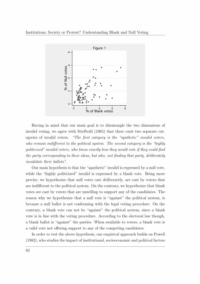
Institutions, Society or Protest? Understanding Blank and Null Voting
0
0
02
2
24
4
46
6
68
8
8% of Null votes
% o
f Nul
l vot
es
% of Null votes0
0
02
2
24
4
46
6
68
8
8% of Blank votes
% of Blank votes
% of Blank votesFigure 1Figure 1
Figure 1
Having in mind that our main goal is to disentangle the two dimensions of
invalid voting, we agree with Stiefbold (1965) that there exist two separate cat-
egories of invalid voters. “The first category is the “apathetic” invalid voters,
who remain indifferent to the political system. The second category is the “highly
politicized” invalid voters, who know exactly how they would vote if they could find
the party corresponding to their ideas, but who, not finding that party, deliberately
invalidate their ballots”.
Our main hypothesis is that the \apathetic" invalid is expressed by a null vote,
while the \highly politicized" invalid is expressed by a blank vote. Being more
precise, we hypothesize that null votes cast deliberately, are cast by voters that
are indi�erent to the political system. On the contrary, we hypothesize that blank
votes are cast by voters that are unwilling to support any of the candidates. The
reason why we hypothesize that a null vote is \against" the political system, is
because a null ballot is not conforming with the legal voting procedure. On the
contrary, a blank vote can not be \against" the political system, since a blank
vote is in line with the voting procedure. According to the electoral law though,
a blank ballot is \against" the parties. When available to voters, a blank vote is
a valid vote not o�ering support to any of the competing candidates.
In order to test the above hypothesis, our empirical approach builds on Powell
(1982), who studies the impact of institutional, socioeconomic and political factors
82
4.1 Introduction
on turnout. In order to have a complete picture of voters' decision not to vote for
any of the candidates, parallel to the decision to cast a blank or a null vote we
include in our analysis the decision to abstain.
Institutional Approach: This approach considers that invalid voting and ab-
stention is a function of the institutional design. A typical example of this category
is compulsory voting. In countries where participation is obligatory, abstention is
lower and voters who would possibly abstain either because of alienation or indif-
ference are obliged to participate and in that case cast an invalid ballot. Other
examples are district magnitude, electoral system, electoral disproportionality,
complexity of �lling the ballot etc.
Socioeconomic Approach: This approach aims to capture how invalid ballots
and abstention are a�ected by the socioeconomic characteristics of the country
or the regions studied. Examples of variables that have been used are wealth of
the country, development, urbanization, education and literacy, number of immi-
grants, social inequality etc.
Political (Protest) Approach: This approach approach captures how invalid
ballots and the level of abstention are a�ected by the characteristic of the electoral
competition and the political situation at the moment of the election. Variables
belonging in this approach are the closeness of the election, the development and
economic performance of the country during the pre-election period, any changes
in levels of democratization, etc.
Empirically, we show that blank and null votes are not a�ected by the same
factors. In particular the presence of an open list has a signi�cant e�ect only
on null votes while the number of strikes a�ects only the percentages of blank
votes. The same holds for compulsory voting since it increases the level of blank
votes while it has no signi�cant e�ect on the level of null votes. Only two of our
variables, the disproportionality of the electoral system and repression of political
rights a�ect both variables in the same way.
In order motivate theoretically our main hypothesis and understand what are
the common and di�erent features of abstaining, casting a blank or a null vote we
build a theoretical model where voters perceive a consumption bene�t of voting
(a la Riker and Ordeshook (1968)) for casting a blank or null ballot. We provide
conditions under which an individual may vote for a candidate, abstain, cast a
83
Institutions, Society or Protest? Understanding Blank and Null Voting
blank or a null ballot. We actually show that the decisions to abstain, vote blank
or vote null are associated with voters that are either indi�erent among parties,
alienated by parties or both simultaneously.
The paper is organized as follows. In section two we present the existing litera-
ture and discuss our contribution to it. In section three we motivate theoretically
why a voter may cast a blank or a null vote. In section four we perform our
empirical analysis and in section �ve we conclude. In the Appendix we provide
descriptive statistics and sources of our data.
4.2 Contribution to the Literature
Invalid voting literature is mainly empirical and consists of two groups of pa-
pers. Earlier approaches studying intra-country variation of invalid voting (Rosen-
thal and Sen, 1973; McAllister and Makkai, 1993; Power and Roberts, 1995; Zul-
�karpasic, 2001) and more recent ones studying cross-country variation of invalid
voting (Power and Garand, 2007; Uggla, 2008).
Regarding single country analyses one of the �rst contributions is by McAllister
and Makkai (1993) for the case of Australia. Their results support the social
structural hypothesis and in particular, invalid votes are explained by the number
of immigrants, since the latter have poor language skills and higher probability
to cast a null ballot by mistake. In a similar analysis for the case of Brazil by
Power and Roberts (1995), the authors show that a model incorporating political,
socioeconomic, and institutional factors is more powerful than a model relying on
any one of these alone4. In the case of provincial elections in Ontario, Galatas
(2008) shows that both demographic characteristics and party competition provide
an explanation for casting blank ballots in a way consistent with expectations of
rational choice theory.
Regarding cross-country evidence, Power and Garand (2007) focus on Latin
American countries and show that variables of all the three approaches shape the
rates of invalid voting. Variables included in the analysis with a signi�cant e�ect
are urbanization, income inequality, compulsory voting, electoral disproportion-
4The institutional approach for intra-country approaches refers to the characteristics of theelectoral system that vary within the country (e.g. district magnitude).
84

4.3 Why Voters Cast a Blank or a Null Vote?
ality, political violence and the level and direction of democratic change. Uggla
(2008) considers an extended panel, and parallel to invalid voting he analyzes vot-
ing for parties that do not reach the threshold required for representation in the
parliament. Uggla concludes that “although at first glance, invalid voting appears
irrational and politically inconsequential, it may in fact reflect political logic”.
Our empirical approach falls in the category of papers providing cross-country
evidence, and the main contribution in the invalid literature, is that we study for
the �rst time blank and null votes on a separate basis.
Rosenthal and Sen (1973) are the only authors providing a theoretical model
of voters' participation decision. As in our setup, they use a spatial model in order
to explain blank votes either because of alienation or because of indi�erence but
they do not aim to approach blank and a null ballots on a separate basis.
4.3 Why Voters Cast a Blank or a Null Vote?
According to the well-known paradox of voting (Downs, 1957) voters should
not be willing to pay the cost of voting and participate in large elections, since
the probability of a�ecting the outcome is tiny. In their seminal work, Riker and
Ordeshook (1968) (R&O) assume that voters obtain a consumption bene�t when
participating in large elections, and hence o�er an explanation of why voters may
do so. R&O actually interpret the consumption bene�t of voting as “the satis-
faction from compliance with the ethic of voting, the satisfaction from affirming
allegiance to the political system, the satisfaction of affirming one’s efficacy in the
political system, the satisfaction of deciding, going to the polls, etc”. When the
bene�t is high enough such that it compensates the cost of voting, it turns out
that the decision of a voter to participate is rational.
In a similar spirit we adapt R&O's approach to explain why a voter decides
to cast a blank or a null ballot. Departing from the standard approach we allow
the consumption bene�t of voting to vary not only among voters but also for
each voter to vary among the available choices. In particular, each voter may
perceive a di�erent bene�t for casting a null vote, a blank vote or a vote for one
of the candidates. A voter casts a blank or a null vote, when he obtains a high
85

Institutions, Society or Protest? Understanding Blank and Null Voting
consumption bene�t of voting, and performing his calculus wants to participate
but is not attracted by any of the competing candidates.
We assume a parliamentary election with two parties j = L;R. Each party is
characterized by its ideal policy xj 2 [0; 1] and a valence characteristic �j 2 [0; 1].
For each voter i, the available strategies are s 2 fj; B;N;Ag and for each voter
each strategy is associated with a consumption bene�t of voting (dSi ). Each voter
is characterized by her ideal point (xi) and her personal cost of voting (ci).
Voters evaluate both policy (xj) and non-policy characteristics (�j) of each
party. The evaluation of party j by voter i is given by: uji = �j � jxj � xij.The total reward that a voter obtains when following strategy s depends on
the consumption bene�t of voting associated with the strategy s (i.e. dsi ), on
the probability of determining the winner of the election (we refer to this as the
instrumental dimension of a voter's decision), and also on supporting a \good"
party in terms of policy and non-policy characteristics (we refer to this as the
expressive dimension of a voter's decision). We assume that voter i puts weight
�i 2 [0; 1] in the instrumental dimension (i.e. (uji � u�ji ) for all j), and weight
(1 � �i) in the expressive dimension (i.e. uji for all j). Thus, �i = 0 describes a
voter deciding in a purely expressive way, while �i = 1 describes a voter deciding
in a purely instrumental way.
The following equation represents the above described reward of individual i
from following strategy s:
Ri(s) =
�ipi(uLi � uRi ) + (1� �i)uLi + di � ci if s = L
�ipi(uRi � uLi ) + (1� �i)uRi + di � ci if s = R
dBi � ci if s = B
dNi � ci if s = N
0 if s = Awhere pi is the probability that the voter will break or create a tie between the
two parties. Having in mind the above speci�cation we can perform the \calculus"
of individual i regarding the decision to abstain, vote blank or vote null.
In order for a voter to abstain the following three conditions have to hold
simultaneously:
1. �ipi(uji � u�ji ) + (1 � �i)u
ji + dji � ci < 0 for both j: The probability of
a�ecting the outcome (pi), the corresponding utility di�erence if one party
86
4.3 Why Voters Cast a Blank or a Null Vote?
wins versus the other (uji �u�ji ), the evaluation of the policy and non-policy
characteristics of the parties (uji ), and the bene�t of voting (di) do not
compensate the cost of participating in the election (ci).
2. dBi �ci < 0: The bene�t from voting blank is not high enough to compensate
the cost of participating in the election.
3. dNi � ci < 0: The bene�t from voting null is not high enough to compensate
the cost of participating in the election.
Given the �rst condition, abstention is increasing in the cost of voting (ci),
decreasing in the bene�t of voting (dji ), decreasing in the probability of a�ecting
the outcome (pi), decreasing in the di�erence of policy and quality characteristics
of the two parties (uji � u�ji ) and decreasing in the evaluation of parties by voters
(i.e. uji ). Fianlly, given the second and third conditions abstention is decreasing
in the consumption bene�t voters obtain for voting blank or null (i.e. dBi and dNi ).
In the literature, the two most common justi�cations of voters' decision to
abstain are that voters are alienated from parties or indi�erent among them.
Notice that the predictions of our model are compatible with both explanations.
The possible indi�erence of a voter is captured by the (uji � u�ji ) term. When
this di�erence is small it implies that the voter is relatively indi�erent among
the parties and hence the probability to abstain is higher. The alienation of a
voter is captured by low evaluations for all parties (i.e. low uji for all j). Since
the probability to abstain is decreasing in uji , according to our model alienated
voters, decide to abstain with higher probability.
Regarding blank voting, the conditions such that a voter casts a blank ballot
are the following:
1. �ipi(uji � u
�ji ) + (1� �i)uji + di < dBi for both j
2. dBi � ci > 0
3. dBi > dNi
Similarly, regarding null voting, the conditions such that a voter casts a blank
ballot are the following:
87

Institutions, Society or Protest? Understanding Blank and Null Voting
1. �ipi(uji � u
�ji ) + (1� �i)uji + di < dNi for both j
2. dNi � ci > 0
3. dNi > dBi
The �rst condition is very similar both for the decision to cast a blank and a
null vote. Both blank and null votes are decreasing in the probability of a�ecting
the outcome (pi), decreasing in the di�erence between the evaluations of the two
parties (i.e. uji�u�ji for all j) and decreasing in the evaluation of parties by voters
(i.e. uji for all j). As in the case of abstention, blank and null votes are associated
both with alienated and indi�erent voters.
Given the second and third conditions both blank and null votes are decreasing
in ci. Blank votes are increasing in dBi and decreasing in dNi while null votes are
increasing in dNi and decreasing in dBi .
Notice that the conditions for a voter to cast a blank or a null ballot are very
similar. In both cases voters are not willing to support any of the parties, and
what determines whether an individual casts a blank or a null ballot is whether
dBi > dNi or dNi > dBi . Hence, the relevant question that we try to answer by
our empirical analysis is the following: When is it the case that dBi > dNi or vice
versa? If we succeed in providing an answer to this question then we may have
an answer to questions such as: Do high rates of blank and null voting portend
citizen dissatisfaction with the political system? Do blank and null votes signify
deficiencies of the electoral system or ballot structure? Do high rates of blank and
null voting portend citizen dissatisfaction with the competing parties?
By de�nition and according to the electoral law, a blank ballot is a vote for
none of the competing candidates and in line with the voting procedure. On
the contrary, a null ballot is a vote not conforming with the rules of the voting
procedure. If a blank and a null vote represent di�erent strategies and indeed
dBi 6= dNi then our hypothesis is as follows: Voter i perceives bene�t dNi that is
higher than dBi when he is not willing to approve the voting procedure and the
democratic institutions. Reinterpreting R&O we hypothesize that a high dNi is
associated with the satisfaction from non-compliance with the ethic of voting, the
satisfaction from not affirming allegiance to the political system, the satisfaction of
88

4.4 Empirical Evidence
not affirming one’s efficacy in the political system, the dissatisfaction of deciding,
going to the polls, etc.
4.4 Empirical Evidence
4.4.1 Data and The Model
Our database consists of 80 lower house parliamentary elections in 14 countries,
for the period 1980-20075. The sample is relatively small but can not be further
extended since the rest of the countries analyzed in the cross-country literature
(Power and Garand, 2007; Uggla, 2008) do not provide separate statistics for
blank and null votes. Detailed descriptive statistics of the dependent variables
and sources of our data can be found in the Appendix.
We follow the empirical literature by estimating a model using variables of
the three de�ned approaches. We suggest that the four dependent variables (i.e.
invalid, blank, null votes and abstention) are a function of institutional, socioe-
conomic and political variables. The main question we try to answer, is whether
there exist a set of independent variables that may a�ect blank but not null votes
and vice versa. As we have explained in the theory the two decisions are distinct
and in order for a voter to choose among the two he must obtain a higher con-
sumption bene�t of voting one versus the other. Estimating the model, we will be
able to see whether di�erent factors in uence each decision or not. The suggested
model is the following:
y = �0+�1Compulsory Voting+�2Disproportionality+�3Open List+�4Real GDP+
�5Democracy Level+�6Closeness+�7Change in Democracy+�8Strikes+�9Growth
where y in the four regressions of interest is the percentage of invalid, blank,
null votes and abstention. Following Powell's classi�cation, the institutional ap-
proach is captured by the three �rst independent variables (compulsory voting,
disproportionality and open list), the socioeconomic approach is captured by the
5The countries that provide separate statistics for blank and null votes are: Argentina,Bolivia, Chile, Costa Rica, Honduras, Iceland, Italy, Netherlands, Paraguay, Peru, Portugal,Spain, Switzerland, Uruguay
89
Institutions, Society or Protest? Understanding Blank and Null Voting
following two (real GDP and democracy level), while the political protest ap-
proach is captured by the last four (closeness of the election, changes in levels of
democracy, number of strikes and growth rate).
Through the institutional variables we aim to answer how institutions a�ect
blank and null voting. Through the socioeconomic variables we focus on charac-
teristics of the society, while though the political protest variables we study how
the characteristics of the election and parties' actions shape blank and null voting.
Institutional Approach
The variables belonging in this approach are meant to answer in what ways
institutions a�ect blank and null voting. This approach includes all those variables
that are not related with parties' actions and the characteristics of the society but
they will rather give us an answer on how voters react to the characteristics of the
institutions. Out of the set of all institutional variables we include in our analysis
the following three: compulsory voting, disproportionality and the presence of
an open list. We believe that those three variables can in general o�er a broad
description of the institutions and in particular the electoral law.
Compulsory Voting: The variable is provided by the International Institute
for Democracy and Electoral Assistance (IDEA) and measures not only presence
but also enforcement of compulsory voting. This variable takes value zero in case
of non-compulsory voting and value three for the case of compulsory voting with
strict enforcement. In our sample in �ve of the countries voting is voluntarily
while in the remaining nine some kind of enforcement applies.
Given that compulsory voting brings to the urns among all voters some that
under non-compulsory voting would have abstained there is evidence that com-
pulsory voting has a positive e�ect on invalid votes (Power and Garand, 2007).
We expect that compulsory voting has a positive e�ect on the percentage of blank
votes since voters not willing to vote for any of the candidates either from alien-
ation (i.e. low uji for all j) or from indi�erence (i.e. low uji � u�ji for all j) can
not any longer abstain.
We expect that compulsory voting has a positive e�ect on null ballots if voters
who are not satis�ed by the electoral procedure (i.e. dNi > dBi ) and in particular
with the obligation to vote are forced to participate.
90
4.4 Empirical Evidence
Regarding abstention, we expect that the stricter is the enforcement for a voter
when he does not participate, the lower should be the level of abstention. This
pattern is the most obvious and prevailing among empirical studies (Fornos et al.,
2004; Blais and Dobrzynska, 1998; Franklin, 1999; Jackman, 1987). Hence, we
expect that compulsory voting has a negative e�ect on the level of abstention.
Disproportionality: In order to measure the disproportionality of the elec-
toral system we construct a disproportionality index following Lijphart and Aitkin
(1994). The index measures the distortion between seat allocation and vote share
obtained for the �rst two parties in the election. High values of the index are asso-
ciated with disproportional electoral systems. In general, disproportional electoral
systems tend to harm smaller parties.
We expect a more disproportional system to be correlated with more blank
votes. Given the small number of parties competing, voters that perceive a high
consumption bene�t of voting and are willing to participate in the election, may
not be able to �nd any attractive alternatives among the competing candidates
and hence decide to cast a blank ballot.
As in the case of compulsory voting, if voters want to show their dissatisfaction
towards the electoral procedure (i.e. dNi > dBi ) and in particular the dispropor-
tionality of the electoral system then we expect a positive e�ect of this variable
on null votes.
We expect that disproportionality has a positive e�ect on abstention. This
is the case because more disproportional systems are associated with less parties
competing in the election and hence less available alternatives for voters (Jackman,
1987; Franklin, 1999; Blais and Dobrzynska, 1998).
Open List: Is a dummy variable taking value one for electoral systems that
allow voters to choose the ranking of candidates, approve a subset of them. etc.
In general it allows voters to \manipulate" the ballot and voting becomes more
complicated than casting a closed ballot. Clearly in countries using an open list
the expected e�ect should be a higher percentage of null votes because of the
higher probability of committing an error.
Regarding blank votes and abstention, this variable should have a negative on
both. This is because in case of an open list voters are o�ered more alternatives
among which they have to choose. Moreover, voters are involved in a more active
91

Institutions, Society or Protest? Understanding Blank and Null Voting
way in the electoral procedure than when they have to vote for a predetermined
list of candidates. The latter may imply higher bene�ts of voting and hence higher
participation in the case of an open list than in the case of a closed list .
Socioeconomic Approach
The two variables of this approach are included in our analysis in order to
explain how the characteristics of the economy (real GDP) and the society (level
of democracy) may a�ect blank and null votes. These two variables describe the
economic and political situation of the country not as a result of parties' actions.
Real GDP: Income per capita is the �rst socioeconomic variable. According to
the empirical evidence turnout is higher in more economically developed countries
(Blais and Dobrzynska, 1998; Norris, 2002; Fornos et al., 2004; Powell, 1982). We
expect real GDP to have a negative e�ect on abstention if high levels of GDP are
associated with more active citizens (and hence on average higher bji ).
Moreover, we expect that higher GDP per capita is associated with less null
ballots cast by mistake. This is because on average, in rich countries, voters'
competency is higher than in poor countries (Power and Garand, 2007).
Level of Democracy: As de�ned by the \Freedom House" this variable takes
value one for high levels of democracy and value seven for autocratic regimes.
We expect more null votes in more autocratic countries. The reasoning is
that in more autocratic regimes voters not voting for any of the candidates are
probably willing to show their dissatisfaction towards the autocratic regime and
institutions through a null ballot rather than showing dissatisfaction towards the
parties through a blank ballot (since dNi > dBi ). If so, the level of democracy
should not a�ect blank voting.
Regarding abstention, we expect that in more democratic regimes, voters par-
ticipate with higher probability. This is because we expect that the consumption
bene�t of voting (bji ) in case of democratic regimes is higher than in autocratic
regimes.
Political Protest Approach
The variables of this approach are included in our analysis in order to capture
the e�ect of the characteristics of the election itself (closeness of the election) and
the e�ect of parties' actions (changes in level of democracy, number of strikes
92
4.4 Empirical Evidence
and growth rate) on blank and null votes. The closeness of the election o�ers a
proxy of the probability that a single vote may be decisive for the outcome of
the election, while the other three variables are included in order to capture the
(dis)satisfaction of voters with parties' actions.
Closeness: This variable measures the competitiveness of the election calcu-
lated as the di�erence between the �rst and second party in the election. This
variable is associated with the pi term of our theoretical motivation. The closer
is the election, the higher is the actual probability of a�ecting the outcome of the
election. If voters have rational expectations then the closeness of the election can
be used as a proxy for the pi term6. According to the predictions of our model,
the lower is pi the higher is the probability that a voter abstains, casts a null or
blank ballot. Hence, we expect a positive e�ect of this variable on all independent
variables.
Change in Democracy: This variable measures the change of political rights.
Positive values are associated with a repression of political rights that during the
period of the last government. Power and Garand (2007) actually show that when
parties repress voters' rights then there is a signi�cant e�ect on the level of invalid
votes. According to our hypothesis, if a repression of political rights is associated
with dissatisfaction towards the parties (i.e. low uji for all j) then this variable
should have a positive e�ect on the level of blank votes. On the other hand,
if voters show their dissatisfaction towards then (un)democratic institutions (i.e.
dNi > dBi ) then we expect a positive e�ect on the percentages of null votes.
Strikes: This variable measures the number of strikes during the last two years.
It is used in our model as a proxy of disapproval towards the parties (i.e. low uji )7.
We use this variable in a similar way that Power and Garand (2007) show that
political violence has a positive e�ect on invalid ballots.
Since this variable captures dissatisfaction towards the political parties, we
6Notice that we proxy the ex-ante probability of being pivotal by the actual electoral outcome.This is a common feature of the empirical literature. We actually assume that voters have apresentiment of the outcome of the election (e.g. through opinion polls) and form expectationsaccordingly.
7We are aware of the fact that the number of strikes may be associated only with dissatis-faction towards rightist governments. Unfortunately, this is the only variable that we could findavailable for all elections and years of our database that can capture the notion of satisfaction.
93

Institutions, Society or Protest? Understanding Blank and Null Voting
expect a positive e�ect of the number of strikes on the level of abstention and blank
votes. If our hypothesis is correct and null votes are used to show dissatisfaction
towards the democratic institutions then we should not expect a signi�cant e�ect
of this variable on the percentage of null votes.
Growth: This variable is computed as the annual change in per capita GDP.
We use this variable as a proxy of economic performance as in the approach by
Power and Garand (2007). The expected e�ect of this variable is the same as of
the number of strikes. We expect that high rates of growth are associated with
high evaluations of parties by voters (i.e. high uji ). Hence, we expect that this
variable has a negative e�ect on the level of blank votes and abstention. It will
have no signi�cant e�ect on the level of null votes, given that according to our
hypothesis the latter are used as disapproval of the democratic institutions.
4.4.2 Empirical Results
A natural question is why the model we estimate combines variables of all the
three approaches rather than studying the e�ect of each approach on each variable
of interest in a separate regression for each approach. We have performed this
task, and concluded that a model combining the three approaches, is associated
with much higher goodness of �t (in terms of adjusted R2) rather than a model
focusing on the e�ect of each approach on each own, both for null and blank votes.
Most important, we observed joint signi�cance of all the independent variables,
in each of the three approaches when analyzed separately, for the case of blank
votes. Hence, all the three approaches have predictive power on blank votes.
This is not true though in the case of null votes. Only institutional variables had
signi�cant predictive power when studied separately. This result, gives us a �rst
hint that blank and null votes are not a�ected by the same factors.
Table 1 summarizes the results of our empirical analysis. In the �rst column the
dependent variable is invalid votes (i.e. the summation of blank and null votes).
In the second and third columns, the dependent variables are blank and null votes
respectively, while in the fourth column the dependent variable is abstention.
As we can see from the �rst column four variables have a signi�cant e�ect on
the percentage of invalid votes. Among the institutional variables, disproportion-
94
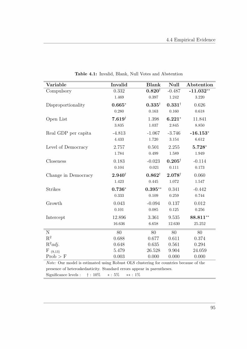
4.4 Empirical Evidence
Table 4.1: Invalid, Blank, Null Votes and Abstention
Variable Invalid Blank Null AbstentionCompulsory 0.332 0.820y -0.487 -11.032��
1.469 0.397 1.242 3.220
Disproportionality 0.665� 0.335y 0.331y 0.6260.280 0.163 0.160 0.618
Open List 7.619y 1.398 6.221� 11.8413.835 1.037 2.845 8.850
Real GDP per capita -4.813 -1.067 -3.746 -16.153�
4.433 1.720 3.154 6.612
Level of Democracy 2.757 0.501 2.255 5.728�
1.784 0.499 1.589 1.949
Closeness 0.183 -0.023 0.205y -0.1140.104 0.021 0.111 0.173
Change in Democracy 2.940y 0.862y 2.078y 0.0601.423 0.445 1.072 1.547
Strikes 0.736� 0.395�� 0.341 -0.4420.333 0.109 0.259 0.744
Growth 0.043 -0.094 0.137 0.0120.101 0.085 0.125 0.256
Intercept 12.896 3.361 9.535 88.811��
16.636 6.658 12.630 25.252
N 80 80 80 80R2 0.688 0.677 0.611 0.374R2adj: 0.648 0.635 0.561 0.294F (9;13) 5.479 26.528 9.904 24.059Prob > F 0.003 0.000 0.000 0.000Note: Our model is estimated using Robust OLS clustering for countries because of thepresence of heteroskedasticity. Standard errors appear in parentheses.Significance levels : y : 10% � : 5% �� : 1%
95
Institutions, Society or Protest? Understanding Blank and Null Voting
ality and an open list have a positive signi�cant e�ect (at 5% and 10% signi�cance
level). The sign is the one expected and is line with the approach by Power and
Garand (2007). The socioeconomic variables have no signi�cant e�ect as in the
case of Uggla (2008). Two of the variables of the political protest approach have
a signi�cant e�ect and is the expected one. More speci�cally, policies repressing
political rights and higher number of strikes are associated with higher levels of
invalid votes (signi�cant at 10 and 5% respectively).
Regarding blank votes, four variables have a signi�cant e�ect and in all cases
the sign is the expected one. Out of the institutional variables, compulsory voting
has a positive e�ect (at 10% signi�cance level) and so does the disproportionality
index. As expected, compulsory voting brings to the urns many voters that ob-
tain low consumption bene�t of voting, are not willing to support any party and
under voluntarily voting would have abstained. These voters under compulsory
voting, once \obliged" to participate, decide to cast a blank vote. Moreover, dis-
proportional electoral systems are associated with more blank votes. A possible
justi�cation may be that the more disproportional the electoral system is, the less
are the competing parties. As a consequence, in disproportional electoral systems,
voters that obtain a high consumption bene�t of voting, are not able to �nd a
party that expresses their ideology, and hence decide to participate and cast a
blank vote.
Out of the political approach, switches to more autocratic regimes and the
number of strikes have a positive e�ect (at 10 and 1% respectively) on blank
votes. In both cases the intuition is the same: dissatisfaction of voters towards
political parties is associated with higher levels of blank votes.
Regarding null votes, four variables have a signi�cant e�ect and all signs are the
expected ones. Out of the institutional variables, disproportionality and an open
list have a positive e�ect (signi�cant at 10 and 5% level respectively). Regarding
the political variables, the percentage of null votes is higher in less competitive
elections (signi�cant at 10% level) while switches to a more autocratic regime are
associated with more null votes as well (signi�cant at 10% level).
Interpreting the results regarding null votes, an open list is associated with
more null votes since the probability that a voter make an error is higher when
he is allowed to manipulate the ballot. In line with our main hypothesis, switches
96
4.4 Empirical Evidence
to a more autocratic regime and disproportional electoral systems are associated
with more null votes as a result of voters dissatisfaction towards the democratic
and electoral institutions (i.e. dNi > dBi ).
In all three regressions (invalid, null, blank) we observe very good �t of our
model to the data (in terms of R2 and adjusted R2). In particular, 68% of the
variance in blank votes, and 61% of the variation of null votes is explained by the
independent variables of our model. In both cases the independent variables are
jointly signi�cant (i.e. prob < 0:000).
Interpreting our results from a comparative perspective, we observe that when
disentangling the two dimensions of invalid voting di�erent variables have a sig-
ni�cant e�ect on blank and null voting. Notice that while compulsory voting has
a signi�cant e�ect on invalid votes, the e�ect comes only from the positive e�ect
on blank votes, since it has no signi�cant e�ect on the level of null votes. In the
same way, only blank votes are increasing in the number of strikes.
The only variable that has a signi�cant e�ect on null but not on blank votes is
the presence of an open-list. This is because an open list captures the null votes
cast by mistake. Contrary to our expectations, an open list does not reduce blank
votes. Our prior that voters have the possibility to choose among more alterna-
tives, and hence cast less blank votes is not con�rmed. Finally, two variables,
disproportionality and changes in levels of democracy, have the same (signi�cant)
e�ect on both blank and null voting.
The most important interpretation of the above results is that information
is lost when the blank and null votes are assumed as the same political action
and one considers only the case of invalid votes. According to our results, under
compulsory voting, when voters are obliged to participate they do not show their
dissatisfaction towards the obligation to vote by casting null ballots, they rather
show their dissatisfaction towards parties through blank voting. In the same spirit
when voters are not satis�ed by parties' policies (as proxied by the number of
strikes), voters show their dissatisfaction only towards the parties through blank
voting. This is not the case though when it comes to repression of democratic
freedom, since after a switch towards a more autocratic regime voters show their
dissatisfaction both by voting blank and null.
Our model is not as successful in explaining the variation of abstention, as it
97
Institutions, Society or Protest? Understanding Blank and Null Voting
is for the case of blank and null voting8. Nevertheless, we believe that the results
of this regression are important. This part of our analysis provides a \robustness"
check of the analysis of blank and null voting. Despite the restricted sample
we study, the results obtained regarding abstention are in line with the much
developed empirical literature. We believe that this gives more credit to the main
results of our analysis, and the conclusion that blank and null ballots are not
a�ected by the same factors.
In particular, abstention is lower in richer and more democratic countries (at
5% sign. level). A straightforward explanation is that voters in rich and highly
democratic countries are more politically active, than voters in poor and auto-
cratic countries. In line with one of the best established empirical regularities,
compulsory voting has a negative e�ect on abstention (at 1% signi�cance level).
Under compulsory voting, voters participate with higher probability in order to
avoid any sanctions.
4.5 Conclusion
In this paper we extend the restricted empirical evidence of the vision of in-
valid voting as a political protest action. Moreover, we make a step forward, by
showing that di�erent factors a�ect the decisions to cast a blank or a null ballot,
and it turns out that information is lost when invalid voting is considere as the
summation of null and blank votes. The kind of questions we aimed to answer
were: Do high rates of blank and null voting portend citizen dissatisfaction with
the political system? Do blank and null votes signify deficiencies of the electoral
system or ballot structure? Do high rates of blank and null voting portend citizen
dissatisfaction with the competing parties? After studying blank and null votes
on a separate basis we conclude that null votes are de�nitely associated with the
ballot structure. Dissatisfaction with the competing parties is associated with
blank votes, while dissatisfaction towards the electoral system and democratic
institutions is associated for di�erent reasons, both with blank and null votes.
An important policy implication of our analysis and a lesson for electoral
8Only 37% of the variation of abstention is explained by the independent variables.
98

4.5 Conclusion
system designers stems from the following result: Compulsory voting has a positive
signi�cant e�ect on the level of blank votes, but has no signi�cant e�ect on the
level of null votes.
This results goes against an important criticism of compulsory voting. Op-
ponents of it, claim that among other issues, compulsory voting is a bad idea,
since it increases the amount of votes that convey no information. If compulsory
voting was associated with more null votes, and given that null votes can always
be attributed to votes cast erroneously, this criticism would have been fair. On
the contrary, it turns out that compulsory voting is associated only with more
blank votes, which are always cast deliberately, can not be misjudged, and actu-
ally convey a doubtless message of voters' disapproval of all competing candidates.
Consequently, compulsory voting does not increase the amount of votes containing
no information. It rather brings to the urns alienated and indi�erent voters, who
are not willing to support any of the competing parties, and once not allowed to
abstain, express their disapproval by casting blank votes.
99
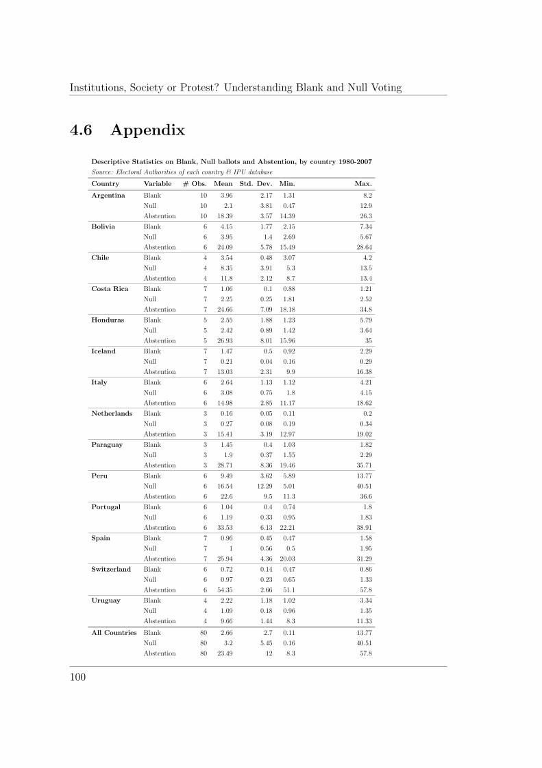
Institutions, Society or Protest? Understanding Blank and Null Voting
4.6 Appendix
Descriptive Statistics on Blank, Null ballots and Abstention, by country 1980-2007
Source: Electoral Authorities of each country & IPU database
Country Variable # Obs. Mean Std. Dev. Min. Max.
Argentina Blank 10 3.96 2.17 1.31 8.2
Null 10 2.1 3.81 0.47 12.9
Abstention 10 18.39 3.57 14.39 26.3
Bolivia Blank 6 4.15 1.77 2.15 7.34
Null 6 3.95 1.4 2.69 5.67
Abstention 6 24.09 5.78 15.49 28.64
Chile Blank 4 3.54 0.48 3.07 4.2
Null 4 8.35 3.91 5.3 13.5
Abstention 4 11.8 2.12 8.7 13.4
Costa Rica Blank 7 1.06 0.1 0.88 1.21
Null 7 2.25 0.25 1.81 2.52
Abstention 7 24.66 7.09 18.18 34.8
Honduras Blank 5 2.55 1.88 1.23 5.79
Null 5 2.42 0.89 1.42 3.64
Abstention 5 26.93 8.01 15.96 35
Iceland Blank 7 1.47 0.5 0.92 2.29
Null 7 0.21 0.04 0.16 0.29
Abstention 7 13.03 2.31 9.9 16.38
Italy Blank 6 2.64 1.13 1.12 4.21
Null 6 3.08 0.75 1.8 4.15
Abstention 6 14.98 2.85 11.17 18.62
Netherlands Blank 3 0.16 0.05 0.11 0.2
Null 3 0.27 0.08 0.19 0.34
Abstention 3 15.41 3.19 12.97 19.02
Paraguay Blank 3 1.45 0.4 1.03 1.82
Null 3 1.9 0.37 1.55 2.29
Abstention 3 28.71 8.36 19.46 35.71
Peru Blank 6 9.49 3.62 5.89 13.77
Null 6 16.54 12.29 5.01 40.51
Abstention 6 22.6 9.5 11.3 36.6
Portugal Blank 6 1.04 0.4 0.74 1.8
Null 6 1.19 0.33 0.95 1.83
Abstention 6 33.53 6.13 22.21 38.91
Spain Blank 7 0.96 0.45 0.47 1.58
Null 7 1 0.56 0.5 1.95
Abstention 7 25.94 4.36 20.03 31.29
Switzerland Blank 6 0.72 0.14 0.47 0.86
Null 6 0.97 0.23 0.65 1.33
Abstention 6 54.35 2.66 51.1 57.8
Uruguay Blank 4 2.22 1.18 1.02 3.34
Null 4 1.09 0.18 0.96 1.35
Abstention 4 9.66 1.44 8.3 11.33
All Countries Blank 80 2.66 2.7 0.11 13.77
Null 80 3.2 5.45 0.16 40.51
Abstention 80 23.49 12 8.3 57.8
100

BIBLIOGRAPHY
Bibliography
Blais, A. and A. Dobrzynska (1998): \Turnout in electoral democracies,"European Journal of Political Research, 33, 239{262.
Downs, A. (1957): \An economic theory of political action in a democracy,"The Journal of Political Economy, 65, 135{150.
Fornos, C., T. Power, and J. Garand (2004): \Explaining voter turnoutin Latin America, 1980 to 2000," Comparative Political Studies, 37, 909.
Franklin, M. (1999): \Electoral engineering and cross-national turnout di�er-ences: what role for compulsory voting?" British Journal of Political Science.
Galatas, S. (2008): \"None of the Above?" Casting Blank Ballots in OntarioProvincial Elections," Politics & Policy, 36, 448{473.
Jackman, R. (1987): \Political institutions and voter turnout in the industrialdemocracies," The American Political Science Review, 405{423.
Lijphart, A. and D. Aitkin (1994): Electoral systems and party systems: Astudy of twenty-seven democracies, 1945-1990, Oxford University Press, USA.
McAllister, I. and T. Makkai (1993): \Institutions, society or protest?Explaining invalid votes in Australian elections," Electoral Studies, 12, 23{40.
Norris, P. (2002): Democratic phoenix: Reinventing political activism, Cam-bridge Univ Pr.
Powell, G. (1982): Contemporary democracies: Participation, stability, andviolence, Harvard Univ Pr.
Power, T. and J. Garand (2007): \Determinants of invalid voting in LatinAmerica," Electoral Studies, 26, 432{444.
Power, T. and J. Roberts (1995): \Compulsory voting, invalid ballots, andabstention in Brazil," Political Research Quarterly, 48, 795.
101
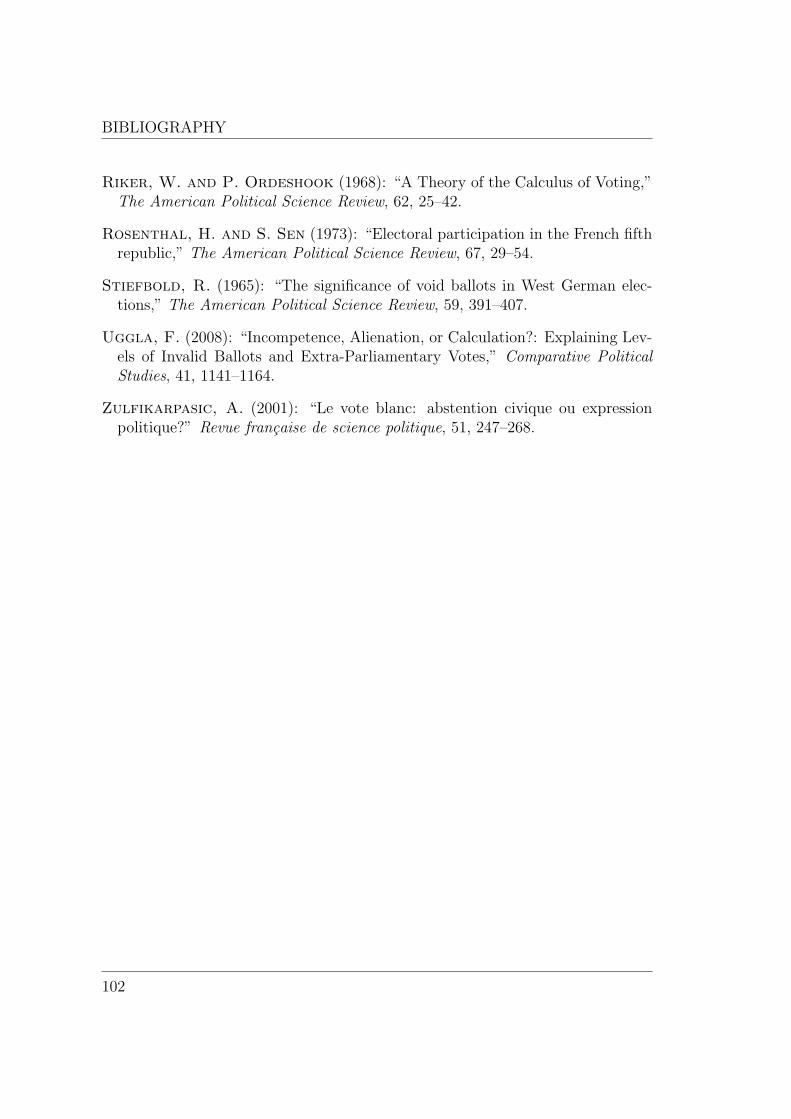
BIBLIOGRAPHY
Riker, W. and P. Ordeshook (1968): \A Theory of the Calculus of Voting,"The American Political Science Review, 62, 25{42.
Rosenthal, H. and S. Sen (1973): \Electoral participation in the French �fthrepublic," The American Political Science Review, 67, 29{54.
Stiefbold, R. (1965): \The signi�cance of void ballots in West German elec-tions," The American Political Science Review, 59, 391{407.
Uggla, F. (2008): \Incompetence, Alienation, or Calculation?: Explaining Lev-els of Invalid Ballots and Extra-Parliamentary Votes," Comparative PoliticalStudies, 41, 1141{1164.
Zulfikarpasic, A. (2001): \Le vote blanc: abstention civique ou expressionpolitique?" Revue francaise de science politique, 51, 247{268.
102