electe=n - defense technical information center security classification of this page a '....

A NEW APPROACH TO CONTROL SINGLE-LINK

FLEXIBLE ARMS. PART II: Control of theTip Position in the Presence of Joint Friction

Vicente Feliu 1, Kuldip S. Rattan 2 and H. Benjamin Brown, Jr.

tolCMU-RI-TR-89-14

ELECTE=N

The Robotics Institute

Carnegie Mellon University

Pittsburgh, Pennsylvania 15213

July 1989

Copyright @ 1989 Carnegie Mellon University

'Visiting Professor, Dpto Ingenieria Eldctrica, Electr6nica y Control, UNED, Ciudad Universitaria. Madrid-28040 Spain

2Visiting Professor. Department of Electrical Systems Engineering. Wright State University, Dayton, OH. 45435.

Ap w.. . .buc .. a..;: 89 10 10169

Unclassified

SECURITY CLASSIFICATION OF THIS PAGE a '.

REPORT DOCUMENTATION PAGEla. RJPT SECL4 TYCLASSIFICATION lb RESTRICTIVE MARKINGS

2a. SECURITY CLASSIFICATION AUTHORITY 3 DISTRIBUTION/AVAILABILITY OF REPORT

Approved for public release;2b. DECLASSIFICATION I DOWNGRADING SCHEDULE distribution unl imi ted

4 PERFORMING ORGANIZATION REPORT NUMBER(S) S. MONITORING ORGANIZATION REPORT NUMBER(S)

CMU-RI-TR-89-14

6a. NAME OF PERFORMING ORGANIZATION 6b OFFICE SYMBOL 7a. NAME OF MONITORING ORGANIZATION

The Robotics Institute (if applicable)

Carnegie Mellon University I6c. ADDRESS (City. State, and ZIP Code) 7b. ADDRESS (City, State, and ZIP Code)

Pittsburgh, PA 15213

8a. NAME OF FUNDINGISPONSORING 8b. OFFICE SYMBOL 9. PROCUREMENT INSTRUMENT IDENTIFICATION NUMBERORGANIZATION (If applicable)

Bc. ADDRESS (City, State, and ZIPCode) 10 SOURCE OF FUNDING NUMBERS

PROGRAM PROJECT TASK WORK UNITELEMENT NO. NO NO. ACCESSION NO

11 TITLE (Include Security Classification)A New Approach to Control Single-Link Flexible Arms. Part II: Control of the Tip Positionin the Presence of Joint Friction

.2 vPE A. eu, .hRattan, and H.R. Brown, Jr.

13a. eTYPE OF.REPPRT 13b. TIME COVERED 114. D T EYF 4MP(T (Year, Month, Day) 15. PA% COUNT

16. SUPPLEMENTARY NOTATI0n:

17. COSATI CODES 18. SUBJECT TERMS (Continue on reverse if necessary and identify by block number)

FIELD GROUP SUB-GROUP

19. ABSTRACT (Continue on reverse if necessary and identify by block number)

This report presents a new way to control the tip position of single-link flexible armswhen friction is present in the joint. In order to mirimize the influence of the nonlinearcomponents of this friction, the control scheme is composed of two lexted loops: an innerloop that controls the motor position, and an outer loop that controls the tip position.

It is demonstrated that proper design of the inner loop of this control scheme eliminates thffects of friction in controlling the tip position, and may significantly simplify the desigof the tip position controller.

Three control schemes are proposed for the outer loop. All of them are based on an hybridfeedforward-feedback control scheme. The first and second schemes use only tip positionfeedback while the third one uses sensing of positions at several points of the beam.

Performances of the three schemes are compared under the following disLurbances: a) rotorposition perturbations, b) unmodelled dynamics, and c) changes in the paylod.-

20. DISTRIBUTION/AVAILABILITY OF ABSTRACT 21. ABSTRACT SECURITY CLASSIFICATION

(JIUNCLASSIFIED/UNLIMITED 0 SAME AS RPT [O1 DTIC USERS Unclassified22a NAME OF RESPONSIBLE INDIVIDUAL 22b TELEPHONE (Include Area Code) 22c. OFFICE SYMBOL

DO FORM 1473,84 MAR 83 APR edition may be used until exhausted SECURITY CLASSIFICATION OF THIS PAGEAll other editions are obsolete

SECURITY CLASSIFICATION OF THIS PAGE

(19 cont'd)

Experimental results are presented for the two arms described in the Part 1; the three tipposition control schemes are compared in both arms; and finally, conclusions are drawn.

SECURITY CLASSIFICATION OF THIS PAGE

kcaeesson for

ceS91Ol aTable of Contents ITIS GRA&IDTIC TA I hiannou.nc ed []

-it I f Ieat I On-

1. Introduction D b 3A': labllitT Codes

2. General Control Scheme Avail and/or 42.1. Description Dist Special 42.2. Feedback Compensation (Sensitivity Analysis) 1 5

2.2.1. Signal-to-noise Ratio Analysis I 62.2.2. Sensitivity to Lh ., dynamic friction coefficient I'I 7

2.2.3. Comparison of the Characteristic Equations 82.3. Feedforward Compensation 9

3. Motor Position Control Loop 93.1. Description and Design 93.2. Decoupling Term 10

4. Motor Control Experimental Results 114.1. Single-Mass Flexible Arm 114.2. Two-Mass Flexible Arm 13

4.2.1. Decoupling from Tip Position Measurements 134.2.2. Decoupling from Intermediate Measurements 14

5. Tip Position Control Loop 155.1. General Scheme 15

5.1.1. Basic Concepts 155.1.2. Error Analysis 16

5.1.2.1. Discretization 165.1.2.2. Analysis 17

5.2. Open-Loop Control 185.2.1. Feedforward Term 195.2.2. Trajectories 20

5.2.2.1. Choosing the Trajectory 215.2.2.2. Designing the Parameters of the Trajectory 23

5.2.3. Considering Inner Loop Dynamics 235.3. Closed-Loop Control 25

5.3.1. Classical Control Using Tip Position Feedback 255.3.2. Control that Cancels the First Natural Frequency by Using Tip Position Feedback 265.3.3. Control Using Feedback of Position at Several Points of the Beam 26

5.3.3.1. Influence of the Payload 27

6. Tip Control Experimental Results 286.1. Single-Mass Flexible Arm 29

6.1.1. Discretization 296.1.2. Open-Loop Control 29

6.1.2.1. Simplified Fcdforward Tcrm 29

6.1.2.2. Complete Feedforward Term 30

6.1.3. Closed-Loop Control Using the First Scheme 30

6.1.4. Closed-Loop Control Using the Second Scheme 31

6.2. Two-Mass Flexible Arm 31

6.2.1. Open-Loop Control 31

6.2.1.1. Trajectory Design 31

6.2.1.2. Feedforward Term 32

6.2.2. Closed-Loop Control Using the First Scheme 32

6.2.3. Closed-Loop Control Using the Second Scheme 32

6.2.4. Closed-Loop Control Using the Third Scheme 33

7. Comparative Study of the Three Tip Position Control Methods 34

7.1. Introduction 34

7.2. Normalization of the Three Schemes 35

7.3. Comparative Study 36

7.3.1. Perturbation in the Tip Position 37

7.3.2. Unmodelled Dynamics 38

7.3.2.1. Open-Loop Control 38

7.3.2.2. Closed-Loop Control 39

7.3.3. Changes in the Payload 40

7.4. Application to our Flexible Arms 41

7.4.1. One Vibrational Mode Case 41

7.4.2. Two Vibrational Modes Case 42

7.4.2.1. Position Disturbances 43

7.4.2.2. Unmodelled Dynamics 43

7.4.2.3. Payload Changes 44

8. Conclusions 44

References 67

ii

List of Figures

Figure 1: Proposed general control scheme. 46

Figure 2: Standard controller for flexible arms (optimum controller). 46

Figure 3: Scheme of Figure 2 expressed in terms of transfer functions. 46

Figure 4: Computer control of the motor position. 47

Figure 5: Closed-loop motor position response using coupling torque compensation,and a Coulomb friction compensation of ±0 amps. (single-mass beam). 47

Figure 6: Closed-loop motor position response using coupling torque compensation,and a Coulomb friction compensation of ±0.09766 amps. (single-mass beam). 47







Figure 13: Closed-loop motor position response using coupling torque compensation,a Coulomb friction compensation of ±0.132 amps., and a limit of 2 mrad. (single-mass beam). 50

Figure 14: Closed-loop motor position response using coupling torque compensation,but not Coulomb friction compensation (single-mass beam). 50

Figure 15: Closed-loop motor position response using a Coulomb friction compensation of±0.132 amps. with a limit of 2 mrad., but not coupling torque compensation (single-mass beam). 50

Figure 16: Magnitude of the frequency responses of the exact and approximate decoupling(expression (32)) in the two-mass beam. 51

iii

Figure 17: Closed-loop motor position response using Coulomb friction compensation of±0.132 amps. with a limit of 2 mrad., and motor-beam decoupling (expression (32))(two-mass beam). 51

Figure 18: Closed-loop motor position response using Coulomb friction compensation of±0.132 amps. with a limit of 2 mrad., but not motor-beam decoupling (two-mass beam). 51

Figure 19: Closed-loop motor position response using Coulomb friction compensation of±0.132 amps. with a limit of 2 mrad., and exact motor-beam decoupling obtained byusing (30) and the Selspot camera (two-mass beam). 52

Figure 20: General computer control scheme. 52

Figure 21: Discretization and reconstruction of the angle of the motor. 52

Figure 22: Simplified computer control scheme. 53

Figure 23: Optimization scheme for the feedforward controller. 53

Figure 24: Simplified feedforward scheme. 53

Figure 25: Parabolic and quasi-parabolic trajectories. 54

Figure 26: Control scheme using tip position feedback. 54

Figure 27: Control scheme cancelling the first vibration mode. 55

Figure 28: Control scheme sensing intermediate points of the beam. 55

Figure 29: Feedforward signal in the single-mass arm case, having neglected motor loopdynamics. 55

Figure 30: Implementation of the complete feedforward term in the single-mass arm case. 56

Figure 31: Feedforward signal in the single-mass arm case, taking into account motorloop dynamics. 56

Figure 32: Tip response of the single-mass arm using the first control scheme. 56

Figure 33: Tip and motor position in the single-mass arm case, using the first controlscheme. 57

Figure 34: Second control scheme in the case of the single-mass arm. 57

Figure 35: Tip response of the single-mass arm using the second control scheme. 57

Figure 36: Tip and motor position in the single-mass arm case, using the second

iv

control scheme. 58

Figure 37: Motor position compared with its reference in the single-mass arm case,using the second control scheme. 58

Figure 38: Quasi-parabolic trajectory and optimized tip i,osition reference in thetwo-mass arm case. 59

Figure 39: Implementation of the simplified feedforward term in the two-mass arm case. 59

Figure 40: Tip response of the two-mass arm using the first control scheme. 59

Figure 41: Motor and tip position in the two-mass arm case, using the first control scheme. 60

Figure 42: Comparison between the feedforward signal and the signal generated by thefeedback controller in the two-mass arm case, using the first control scheme. 60

Figure 43: Implementation of the second control scheme in the two-mass arm case. 60

Figure 44: Tip response of the two-mass arm using the second control scheme. 61

Figure 45: Tip and middle mass position in the two-mass arm case using the secondcontrol scheme. 61

Figure 46: Motor and tip position in the two-mass arm case, using the second control scheme. 61

Figure 47: Comparison of the actual and the commanded motor position of the two-massarm using the second control scheme. 62

Figure 48: Feedforward signal for the two-mass arm in the second control scheme. 62

Figure 49: References for the different angles of the two-mass arm using the thirdcontrol scheme. 62

Figure 50: Tip response of the two-mass arm using the third control scheme. 63

Figure 51: Middle-mass position and its reference in the third control scheme. 63

Figure 52: Motor, middle-mass, and tip position in the two-mass arm case, using thethird control scheme. 63

Figure 53: Normalized first control scheme. 64

Figure 54: Normalized second control scheme. 64

Figure 55: Normalized third control scheme. 64

Figure 56: Motor disturbance applied to the first control scheme. 65

V

Figure 57: Characteristic that compares sensitivities of schemes I and 2 tounmodelled motor loop dynamics in the single-mass arm case. 65

Figure 58: Characteristics that compare rejection properties to motor positionperturbations of schemes 1 and 2, and 1 and 3 respectively, in the case of the two-massarm. 66

Figure 59: Characteristic that compares sensitivities of schemes I and 3 to changesin the tip mass, in the two-mass arm case. 66

vi

List of Symbols

A n x n constant matrix used in the dynamic model of the beam.

A n x n constant matrix used in the state space model of a system.

a(s) analog controller of the motor position control loop (feedforward term).

a(z) discrete compensator for the feedforward term of the motor position control.

ao independent term of a(z) controller.

a, term in z- 1 of a(z) controller.

ai minimum phase zeros of the tip - motor position transfer function.

a,,, : element of the first row - first column of matrix A.

5 : n x I constant matrix used in the dynamic model of the beam.

B : n x 1 constant matrix used in the state space model of a system.

b(z) : discrete compensator for the feedback term of the motor position control.

bo independent term of b(z) controller.

b :term in z- 1 of b(z) controller.

bi: non-minimum phase zeros of the tip - motor position transfer function.

b, first element of vector S.

C I x n constant matrix used in the state spac model of a system.

C(s) : transfer function between the beam deflection from basis to tip and the coupling torque.

Co constant approximation of C(s).

Ci 1 x n constant matrix used to define the transfer function between mass mi position andmotor position.

CF: Coulomb friction.

C, motor - bcam coupling torquc.

vii

C7'(s) : coupling torque estimated from the basis to tip deflection of the beam, and the transfer function

C(s).

D : number of sampling periods of delay of the transfer function of the inner loop.

d(s) : denominator of the tip - motor position transfer function.

E elasticity coefficient of the beam.

e: error between the desired trajectory and the trajectory feasible using a bounded control signal.

eo, :tracking error of the closed-loop system when following the desired tip trajectory.

e6 errors in the tip position due to perturbations.

F, extmal force applied to the tip of the beam.

F(s) transfer function of the feedforward term of the tip control scheme of Figure 1.

f(z) discrete transfer function of the correction term used in the feedforward tip control term tocompensate for inner loop dynamics.

f,(z) numerator of f(z).

fd(z) denominator of f(z).

f (s) transfer function of the filter used to generate the optimum feasible trajectory for the tip fromthe desired trajectory.

: matrix of transfer functions (closed-loop system) between the desired trajectories for the measuredpoints of the beam and the actual measurements.

G(s) generic continuous transfer function.

G(z) equivalent discrete transfer function of G(s).

GI(s) closed-loop transfer function between a motor perturbation and the tip position in the first controlscheme.

G2(s) closed-loop transfer function between a motor perturbation and the tip position in the secondcontrol schcmc.

G3(s) closed-loop transfer function between a motor perturbation and the tip position in the thirdcontrol scheme.

g,(s) transfer function between the tip and motor positions.

g,,(s) numerator of the transfer function between the tip and motor positions.

viii

g,,(s) :denominator of the transfer function between the tip and motor positions.

,,(s) :transfer function of the optimum feedforward term.

~z- 1) :transfer function of the discretized version of the optimum feedforward term.

,,,(z-1) :numerator of k,,(z- 1).

,,(z- 1) :denominator of k,,(z-').

gn grouping of all the minimum phase factors of g,(s) • gn(-s).

gn : grouping of all the non-minimum phase factors of g,(s) • g,(-s).

kni coefficient of order i of the polynomial part of k,(s).

k,,p(s) : proper rational function part of k,,(s).

gni : n row - i column element of the transfer functions matrix (.

g'(s) transfer function resulting from closing the positive feedback loop (second control scheme) inthe single-mass beam example.

g'(s) transfer function resulting from closing the positive feedback loop (second control scheme) inthe two-mass beam case.

gn'(s) transfer function resulting from closing the positive feedback loop (second control scheme) andcancelling the minimum phase dynamics in the two-mass beam case.

R : I x n constant matrix used in the expression of the motor - beam coupling torque.

hi (1 < i < n) : elements of matrix R.

h, l :coefficient that expresses the influence of the motor angle on the motor - beam coupling torque.

h,2 :coefficient that expresses the influence of the external torque applied to the tip of the arm onthe motor - beam coupling torque.

I cross-section inertia of the beam.

In identity matrix.

Iuu(s) transfer function obtained from the input of the beam system u(t) by multiplyingu(s). u(-s).

I+IIuu(s) grouping of all the minimum phase factors of Ilujjs).

ix

I-u(s) : grouping of all the non-minimum phase factors of Iuu(s).

i* motor current.

i, feedforward current term used to compensate for Coulomb friction and motor-beam coupling.

it: part of the motor current that moves the linear part of the system (i less the current wasted inCoulomb friction).

1(s) : current that moves the linearized and decoupled motor (i = i - i,).

3 cost index used in optimization problems.

J. inertia of the motor.

j" imaginary number.

K: electromechanical constant of the D.C. motor.

K": gain of the transfer function between motor and tip position.

K, :I x n feedback vector that represents the controller used to place the closed-loop poles of thesystem.

K, part of K, that weights the influence of states others than the tip position in the control.

k : integer used to represent sampling instants.

k¢i : element of K, that weights the influence the tip position in the control.

L(s): generic transfer function of a closed-loop system, used in sensitivity analyses.

.A : n x n diagonal constant matrix that represents the influence of masses mi on the dynamics ofthe beam.

M(z) : discrete transfer function of the motor control loop.

ml I < i < n : lumped mass at position i.

mn, :lumped mass at the tip of the beam.

m ° • nominal lumped mass at the tip of the beam.

m(s) : transfer function of the motor after having removed the effects of Coulomb friction.

ih(s) : transfer function of the motor after decoupling and linearizing by using i.

N(z) : discrete transfer function of the feedforward term of the first control scheme.

'C

n: number of oscillation modes.

i: number of states of a system.

n,, :order of the denominator of gn(s).

n, number of minimum phase zeros.

n2: number of non-minimum phase zeros.

n, order of polynomial F_ s in expressions (48) and (49).

n,, :number of parameters of the inner loop transfer function.

n, number of zeros of M(z) that are outside the unit circle, or are real negative.

P(s) : polynomial in s vector that defines the influence of the tip position measurement in thereconstruction of the state vector of the flexible arm (expression (5)).

Pp : reference trajectory, without considering non-minimum phase corrections.

p : parameter used to model the dynamics of the single-mass flexible beam (expressions (96) and (97)).

Q(s): polynomial in s vector that defines the influence of the current measurement in the reconstructionof the state vector of the flexible arm (expression (5)).

R(s) : closed-loop controller of the tip position.

R(z) : discrete version of the closed-loop controller of the tip position.

R(s) • closed-loop controller of the tip position using the standard pole placement design metho.'.

RI 2 • n x 2 • n state weighting matrix in the optimization of the tip feedback controller.

R2: constant that weights the control signal (motor angle) in the optimization of the tip feedback controller.

r1,0 : independent coefficient of the P.D. controller used in the first control scheme for the single-massbeam.

r1,1 : first order coefficient of the P.D. controller used in the first control scheme for the single-massbeam.

r2,o : independent coefficient of the P.D. controller used in the second control scheme.

r2, :first order coefficient of the P.D. controller used in the second control scheme.

SL,, : sensitivity of transfer function L to changes in parameter IL.

xi

ST,mM . sensitivity of transfer function T to changes in the tip mass.

ST,,,, :sensitivity of the i-scheme to changes in the tip mass.

ST, CI sensitivity of transfer function T to changes in the parameter i of the inner loop.

s : Laplace transform variable.

T: sampling period.

T, : external torque applied to the tip of the arm.

T(s) generic transfer functions.

Ti(s) transfer function of the i-scheme.

t : time.

U(z) factor of the feedforward term that is 1 if the perfect inversion of the arm dynamics ispossible. If not, it is a discrete transfer function close to 1 (if the feedforward term is welldesigned).

u(s) laplace transform of the input to the beam transfer function.

V : dynamic friction of the motor.

W(z) : rational function in z used to express the condition that the feedforward term must follow secondorder parabolas without any steady state error.

W,(z): polynomial in z- .

Xl(z - 1 ) : z-factor of the hold in computer control systems.

X2(s) numerator of the s-terms of the hold in computer control systems.

X3 (s) denominator of the s-terms of the hold in computer control systems.

x states of the system.

xi: i-state.

x, vector reference of the states.

1(t) : feedforward signal.

Z : discretization function.

xii

z : z-transform variable.

z. positive zero of g,(s) transfer function.

a': vector of dimension n, of parameters of the inner loop transfer function.

a' ° vector of parameters of the inner loop transfer function in the nominal conditions(M(s) = 1).

ai coefficients of the second order factor that appears in the numerator of filter (49).

a, : absolute value of the zeros of the two-mass flexible beam.

cei element i of the vector of parameters of the inner loop transfer function.

-y : control signal generated by the feedback controller of the tip position.

6(z) : discrete transfer function that represents the perturbations of the system.

&(z) "numerator of 6(z).

6 1 : amplitude of the perturbation in the motor position (step).

61(s) • transfer function of the perturbations in the motor position (the same as e).

62(S) : transfer function of the perturbations in the tip position.

E(s) • transfer function of the perturbation current applied to the motor in the robustness analysis ofthe nested loop scheme.

e(s) : perturbation in the motor angle (the same as 61).

Si - th closed-loop pole od Scheme j.

9 • vector of dimension n that represents the angular positions of the lumped masses of thebeam.

• vector of dimension n that represents the angular velocities of the lumped masses of thebeam.

69, • position reference of the lumped masses.

Oi I < i < n • angular position of mass mi.

Oi I < i < n • angular velocity of mass mi.

0.. motor angular position.

xiii

0,, :reference of the motor angular position.

e,,, : feedforward signal for the tip control.

0., angular position of the tip.

0,,: reference of the angular position of the tip.

A: 2 . n row vector that represents a "P.D. type" feedback controller for the tip position, in thethird control scheme.

A, : n row vector that represents the "P." terms of the feedback controller for 'he tip position,in the third control scheme.

A2 : n row vector that represents the "D." terms of the feedback controller for the tip position,

in the third control scheme.

ij :ratio between the sensitivity to changes in the tip mass of control schemes i and j.

M : changing parameter in the sensitivity analysis.

v : difference between the orders of numerator and denominator of gn(z- 1 ) -. (z-I).

r 7r number.

p: ratio between the output component due to the input command and the output component dueto perturbations.

Pid :ratio between the effects of motor position perturbation in schemes i and j.

ei : zeros of the inner loop discrete transfer function that are outside the unit circle or are realnegative.

"i, :ratio between the sensitivity to unmodelled motor control loop dynamics of control schemes iand j.

Y : n column vector of transfer functions that relates the references for the position of masses miwith the reference for the tip angle.

X(s): transfer function that represents the coupling between the motor and the beam in the motortransfer function.

O(s) : transfer function that relates the angle of the motor with the motor-beam coupling torque.

l, w 2 : first and second vibrational modes of the two-mass flexible beam in rad/sec.

* variables are also used as integer indexes to represent elements of other vectorial variables.

xiv

Abstract

This report presents a new way to control the tip position of single-link flexible arms when frictionis present in the joint. In order to minimize the influence of the nonlinear components of this friction,the control scheme is composed of two nested loops: an inner loop that controls the motor position, andan outer loop that controls the tip position.

It is demonstrated that proper design of the inner loop of this control scheme eliminates the effectsof friction in controlling the tip position, and may significantly simplify the design of the tip positioncontroller.

Three control schemes are proposed for the outer loop. All of them are based on an hybrid feedforward-feedback control scheme. The first and second schemes use only tip position feedback while the thirdone uses sensing of positions at several points of the beam.

Performances of the three schemes are compared under the following disturbances: a) motor positionperturbations, b) unmodelled dynamics, and c) changes in the payload.

Experimental results are presented for the two arms described in the Part I; the three tip positioncontrol schemes are compared in both arms; and, finally, conclusions are drawn.

I I I I I I2

1. Introduction

Very little effort has been devoted to the control of flexible arms when static and dynamic frictionsare present in the joints, in spite of this being common in practice, as was mentioned in the GeneralIntroduction (see the first report of this serie of three). The effects of friction are especially important inlightweight flexible arms, or in flexible arms moving at low speeds and accelerations.

In this second report, control of single-link flexible arms with friction in the joint is studied. A generalcontrol scheme is proposed in Section 2 to compensate for it. Existing methods to control flexible arms[1-6] are based on explicit control of the tip position. In these schemes, the controller generates a controlsignal, which is the current (after being properly amplified), for the DC motor that drives th.o arm. Wepropose here a new method which is based on the simultaneous control of the joint motor position andtip position, and the implementation of two nested closed loops: an inner loop that controls the motorposition and another outer loop that controls the tip position. In our scheme, the tip position is controlledby using the motor position instead of the current as control signal. Friction is compensated in our schemeby using controllers of high gains in the inner loop. It is demonstrated that this can be done even in thecase in which the arm is non-minimum phase.

Section 3 describes the design of the inner loop controller. Compensation of Coulomb friction andthe coupling torque between the motor and the beam is carried out. It is stated that, in many cases, thedynamics of the motor position control loop is negligible compared to the dynamics of the beam (secondsubmodel in Section 2 of Part I). This allows us to simplify the design of the outer loop. Section 4presents the experimental results obtained when closing the inner loop in the cases of two lumped-massflexible arms that we have built in our laboratory: a single-mass arm, and a two-mass arm (they weredescribed in Part I). Because the first arm is minimum phase and the second non-minimum phase, all thepossible cases of single-link flexible arm control are included in our experiments.

The outer control loop is described in Section 5. Three control schemes for the tip position treproposed in this report: two schemes based on classical frequency domain techniques, and a third schemebased on state-space methods. All three schemes combine a feedforward term with a feedback controller.It is shown that, with this hybrid feedforward-feedback scheme, high position accuracy may be achievedfor the tip of a flexible arm. The feedforward term is designed to drive the motor in such a way that thetip of the arm approximately follows the desired trajectory. The closed-loop controller compensates forthe deviations of the tip from the nominal trajectory. If the feedforward term is properly designed, theseerrors are small, allowing us to use simple controllers. The feedback control law is implemented in thetwo first schemes by sensing the tip position. The feedback law of the third scheme uses sensing of theposition in several intermediate points of the arm. The second method exploits a special feature that thegeneral control scheme proposed here exhibits: the first (lowest) natural frequency of the beam, which isthe dominant one, may be easily cancelled by closing a positive feedback loop of the tip position.

Are presented in Section 6 experimental results of tip position control, that were obtained applyingthe three methods to our two flexible arms. Performances of the three schemes are compared in Section7 under the following disturbances: a) motor position perturbations, b) unmodelled dynamics, and c)changes in the payload are present.

Finally, conclusions are drawn in Section 8.

3

2. General Control Scheme

2.1. Description

As it was mentioned in the introduction, there are many applications in which the friction must betaken into account when controlling a flexible arm. Only when friction torque is much smaller than beamtorque, can it be ignored. This happens in cases such as very large flexible structures, or direct-drivearms designed for minimum friction.

Several methods have been proposed to minimize the effects of friction in the control of DC motors,that can be directly applied to the control of rigid arms. The simplest method is to use a high-gain linearfeedback. This is based on the property that the robustness of a closed loop system to perturbations andchanges in its parameters is improved when the open loop gain is increased (Kuo [7]). This has beenused by Wu and Paul [8], for example. The main limitation of this method when applied to rigid armsis that the nonlinearities will dominate any linear compensation for small errors tending to give smallpermanent errors in the positioning. More significant limitation appears when this is applied to control offlexible arms, which are typically non-minimum phase systems. This means that a high-gain tip positionloop leads to system instability (this is consequence of having the system zeros in the righ half-plane).Consequently, this method is unsuitable for flexible arms.

Another method for compensating friction is the use of force sensors and the mechanization of afeedback loop around the motor torque. Examples are Handlykken and Turner [9], and Cannon andSchmitz [1] (the latter is an application to flexible arms). Finally, other methods are based on the use ofa calculated compensation term which is added to the current of the motor in order to compensate thefriction torque. Examples are Walrath [10] that used a model of the friction in order to predict its value,and more recently Canudas et al. [11] that used a parameter identification procedure (a recursive leastsquares algorithm) in order to obtain this term.

In this section we propose a new simple control scheme to reduce the effects of the friction. Thisscheme is based on a modification of the classical high gain position closed loop procedure, in order toallow its application to flexible arms. This method does not need extra sensors (to measure the torque ofthe motor) and allows much simpler calculations than other compensation methods. Our control schemealso incorporates a constant feedforward term in order to remove the remaining steady state errors becauseof the Coulomb friction. This method practically eliminated friction nonlinearities in our flexible arms.

In order to reduce the effects of the friction, the basic control scheme of Figure 1 is proposed. Thisscheme has two variables: motor and tip positions: 0,, and 9 respectively (using the nomenclature definedin Figure 1 of Part I). These two variables are controlled by two nested closed loops, and two differentcontrollers (R(s) and a(s)) are used, each one being designed separately according to different criteria. InFigure 1, r(s) is the motor open-loop transfer function between the current and the angle of the motor. Itis easy to show that m(s) always has all its poles and zeros in the left half-plane. The open-loop transferfunction of the flexible beam gn(s) relates the angle of the tip of the beam to the angle of the motor.gn(s) has all its poles in the left half-plane but may have (for arms with more than one vibrational mode)some zeros in the right half-plane (non-minimum phase system). F(s) is an open-loop term designed inconjunction with R(s).

Existing control schemes for flexible arms basically generate a current for the DC motor as functionof the tip position error and/or its derivatives. If we try to compensate for friction in these schemes,by increasing the gains of the controller, the closed-loop system becomes unstable because of the right

4

half-plane zeros of g,(s). But in our proposed scheme, because m(s) is minimum phase, the gains for theinner loop can be arbitrarily increased (using an appropiate controller a(s)) without making the systemunstable. So, intuitively, the high gain inner loop that controls the motor position makes the systeminsensitive to the friction and, then, a second outer loop may be designed to control the tip position. Thissecond loop cannot have a high gain because gn(s) is non-minimum phase, but now it does not matterbecause the friction effects have been nearly removed by having closed first the high gain inner loop.

2.2. Feedback compensation (sensitivity analysis)

The previous ideas justify intuitively the interest of using our control scheme. This subsection givesanalytical proof of it (Rattan et al. [12]). The analysis carried out here is quite straightforward and willgive a quantitative idea of how much the robustness to friction is increased by using our nested multipleloop scheme. In order to do this comparison, a typical control scheme like the one shown in Figure 2 willbe used (Cannon [1], a.e.). The sensitivity characteristics of this system will be taken as representativeof the exisung methods because they are based on controlling the tip position using only a controller thatgenerates a command for the current of the DC motor. So the sensitivities of all them are of the sameorder of magnitude. Two comparative analyses will be carried out: one checking the signal-to-noise ratio(considering that the Coulomb friction is the noise), the other checking the sensitivity to variations in thedynamic friction coefficient.

In order to do these comparative analyses, we first express the state space control scheme of Figure 2in terms of its equivalent transfer functions.

Assume that the plant is represented by the state space equations:

.t(t) = A . x(t) + B . it(t), (1)

O(t)=C.x(t); C= ( 1 0 0 ... 0 (2)

the system being of dimension h. it is the part of the current given by the controller and actuator, whichis applied to the linear part of the model. The remaining quantity of i(t) is used to compensate for jointfriction. Assume also that the controller is a row vector of dimension h of the form:

where 1, is a vector of dimension i - 1, and kI1 is the coefficient corresponding to the feedback of thetip position error (error in the first state).

Differentiating the state space equations h - I times we get:

5

C-AX(°)AJ (EflLA -I C A2

Observability Matrix

0o o o.. 0 0CoB 0 0 ... 0 0

C.A.B C-B 0 ... 0 0IiJ (4)

C.-A" - 2 . B C.A - - B C.A - - B .. C.B 0 i,-

and if the system is observable (which is true in all the models of flexible arms), then the states x of thesystem may be reconstructed from measurements of the input ij and the output 0,, using a linear law ofthe form:

x(s) = P(s) .O(s) + Q(s) . ij(s) (5)

where P and Q are polynomial in s column vectors. This last equation is easily obtained from (4) byinverting the observability matrix. Substituting this ix the scheme of Figure 2, substituting also the statespace equation of the plant by gn(s) r m(s), and operating we get the equivalent transfer function schemeshown in Figure 3. In this figure:

F*s re(s), g,(s)F(s) = P(s) m(s) . g.(s) + Kc . Q(s)' (6)

and

R(s) =-Kc . P(s) . m(s) . gn(s) + Kc " Q(s)r(s) gn(s) (7)

Now, the comparative analysis may be done between the schemes of Figures 1 and 3.

2.2.1. Signal-to-noise ratio analysis

The signal-to-noise ratio of the output of a system is defined (Kuo [7]) as:

Output due to signal

Output due to noise'

and is a measure of the insensitivity of the system to perturbation signals (in this case Coulomb friction).

6

The comparison of the ratios of the schemes of Figures 1 and 3 is done here, for the same levels of input,0, and perturbation E (which is added to the current of the motor).

Operating the nested double loop scheme we get from Figure 1 that:

0,(s) = M(S) g.( - ~s) r(s) g,-(s) + c(s)). (9)1 + r(s) a(s) + gn(s) , m(s) . R(s) . a(s)

And the signal-to-noise ratio for this scheme easily follows:

po,, = R(s) .a(s) .F(s). (10)

We get from Figure 3 that

,.(s) +r(s) g,.(s) • (R(s). F(s)O,,(s) + ((s)) (11)1 + g.(s), rn(s), R(s)

Po,., = R(s) . F(s) = k, 1 . (12)

Comparing both results, expression (10) may be made very large because the gains of controller a(s)may be designed arbitrarily high. But k,1 in expression (12), and all the parameters of R(s) in general,are limited by the stability margin because the system is non-minimum phase. The gains of R(s) ofFigure 1 are limited for the same reason too. Therefore, expression (10) may be made larger than (12)in general, just by choosing properly the gains of the controller of the inner loop. In practice, the gainsof the inner loop will be limited by the saturation of the amplifier, unmodelled high frequency dynamics,or discretization of the signals when using digital controllers. But in general case these limits are muchlarger than the ones imposed by the non-minimum phase characteristic.

2.2.2. Sensitivity to the dynamic friction coefficient

Dynamic friction is another component of friction. It is normally assumed to be linear, and it is in-cluded in the model of the plant. Often, however, the dynamic friction coefficient changes noticeablydcpending on the sense of rotation of the motor (see Figure 8 of the first report), or the position of therotor relative to the s:ator (confronted poles), etc. Performing the sensitivity analysis of both systems tochanges in the dynamic friction coefficient, we show here that the robustness to this parameter may besignificantly improved also using our nested double loop scheme.

The sensitivity of a system, whose closed-loop transfer function is L(s), to changes in a parameter it,is defined (Kuo [7]) as

OL(s) itSt.., = l "L~s--' "(13)

Opt L(s)

The motor submodel is described by (sec Subsection 2.2 of Part 1):

7

d2 0m d~rmK. i =J .!to m +V. m + C,+CF (14)

dt2 dt

Ct = " (9 + h,+l - 0,, + hn+2 • Tn (15)

In order to do this analysis, we assume that CF and T, are 0; and, from (14),(15), we express r(s) inthe form:

Krn(s) = s2 + V., (16)

which is the typical transfer function of a DC motor with the exception of the term \(s), that representsthe coupling between the beam and the motor. This allows us to characterize the influence of the dynamicfriction coefficient V in the general transfer function.

Carrying out some calculations, we obtain that the sensitivity to V of the closed-loop system of FigureI is:

SLY -S. V (17)(1 + a(s) . m(s) . (I + R(s) • g,(s))) . (J . s2 + V. s + X (s))(

The sensitivity to V of the system of Figure 3 is:

SLV =-S. VS.v=(I +R(s) • me(s),- g,(s)) . (J. s2 + V. s + X((s))" 8

Comparing both sensitivities, expression (17) will normally be significantly smaller than (18) becausea(s) • (1 + R(s) • g,(s)) >> R(s) • g.(s). Notice again that the gains of R(s) and R(s) are bounded by astability margin, but the gain of a(s) may be increased arbitrarily. Consequently, scheme of Figure 1 ismore robust in general to changes in the dynamic friction than the scheme of Figure 3, by a factor ofapproximately a(s).

2.2.3. Comparison of the characteristic equations

The previous analysis gives a quantitative justification of how the robustness of the system is increasedusing the two nested loops schemc. A bceacr 4ualita'"ve understanding of how the nested loops modifythe stability of the system, allowing higher gains, may be obtained just by looking at the characteristicequations of the two systems.

In the standard control scheme, the robustness depends on /(s), and the characteristic equation is

1 + R(s) ms) • gn(s) = 0;

8

or, substituting R(s) by (7) in this equation:

& . P(s)1+ m(s).- g'()IK (s) = 0, (19)

which expresses the characteristic equation in terms of me feedback gains. Notice that, in this lastequation, the right half-plane zeros of gn(s) limit the gains K, and, consequently, the gains of R(s).

In the proposed scheme we have, from equation (10), that the signal-to-noise robustness depends onthe product a(s) R(s); and, from equation (17), that the sensitivity depends on this product and alsodepends on an a(s) term. The characteristic equation of the system is:

1 +a(s). m(s) • (1 +g.(s).R(s)) = 0. (20)

and, if the factor I + gn(s) -R(s) had all its zeros in the left half-plane, then the gains of a(s) could bemade arbitrarily large. Because gn(s) is stable, there always exists an R(s) of moderately low gains thatmakes the mentioned factor have all its zeros in the left half-plane (this may be justified from the rootlocus plot of gn(s) R(s)) and, consequently, the product a(s) R(s) may be arbitrarily large improving therobustness of the system.

2.3. Feedforward compensation

The scheme of Figure 1 overcomes the stability problems which are caused when implementing highgain feedback loops in non-minimum phase systems in order to increase its robustness to friction. Butstill small steady state errors may be present.

A feedforward term can be added to the current of the motor to remove this. This term is a constantone that changes its sign depending on the sign of the motor velocity. This term is used to compensate foran ideal Coulomb friction torque, and the value used here is the averaged one given by the identificationmethod described in Section 5 of Part I.

3. Motor Position Control Loop

3.1. Description and Design

A main objective of the inner loop design is to remove the modelling errors and the nonlinearitiesintroduced by the friction by means of very high gains. Another important goal is to make the responseof the inner loop significantly faster than the response of the outer loop and, of course, very much fasterthan the motions produced by the vibrational modes of the arm. This will simplify the design of the outerloop. In fact, if the inner loop is relatively fast we can substitute for the inner loop of Figure 1 a blockwith unity transfer function. This allows us to study the flexible arm just as a system of g,(s) transferfunction whose control signal is the angle of the motor.

In order to design the controller of the inner loop, three approaches may be used. provided that a

feedforward term is used to compensate for the Coulomb friction:

1. Design a regulator to control the linear part of the motor submodel (16). This part is minimumphase but may be quite complex, even having zeros in the imaginary axis.

2. Consider the coupling torque between the motor and the beam just as another perturbation, anddesign a regulator to control the reduced equation obtained from (16):

d2 Om(t) d~m(t)K. i(t) = J. t) V. d- (21)

3. Design a regulator to control the system represented by (14),(15), but using another feedforwardterm to compensate for the coupling between the motor and the beam. This may be estimated frommeasurements of a strain gauge installed in the basis of the beam, or can be calculated from themeasurements of the angles of the motor and the tip, by using (15).

We use the third approach because it simplifies the design of the inner controller, and because wewant explore the posibilities of estimating the coupling torque from measurements of the motor and tipposition. Because the control is robust, an approximate estimation of this torque is adequate. The errorsproduced by this approximation will be compensated by the high gain inner loop. These points will bedeveloped in the next subsection, and illustrated by the experiments of Section 4.

Assume in what follows that we are able to calculate by some method the coupling torque C, betweenthe motor ard the beam. Then the system may be approximately decoupled and linearized by adding tothe current the following term:

i,(t) = (CI(t) + CF(sign of motor velocity))/K. (22)

Then the motor transfer function used to design the controller is reduced to the typical one for DCmotors:

Ore(S) _ K/J 23OM.s = I = h(s). (23)is s, (s + v/r)

A digital controller of the form shown in Figure 4 is suggested in order to get a very fast responsewithout overshooting. This figure represents the inner loop to control the motor position, where 0,,, isthe commanded motor position, and a(z) and b(z) are phase-lead controllers. The limits in the gains ofa(z) (resembling a(s) of Figure 1) depend upon the current limit of the amplifier of the DC motor as wellas beam deflection limits. In the cases where the coupling torque is high, it is necessary to take intoaccount in the design the current drained by the coupling 9o.npensation term. This will lower the valueof the maximum current that is available for the feedback control of Figure 4. A delay term is includedin this scheme in order to take into account the delay in the control signal because of the computations.

3.2. Decoupling term

Coupling torque C, can be exactly compensated by using expression (15), if measurements of all the

10

angles 0.,01,...,0. are available (we assume in what follows that T. is 0). But often, we only havemeasurements of the motor angle 0.. and the tip angle 0. Under these circumstances, the coupling torquehas to be approximated from an expression

C't(s) = C(s) . (0.(s) - On(s)), (24)

where C(s) is a transfer function to be designed.

If we denote

C(s) = tp(s) ,,(s); (25)

then the C(s) that exactly compensates the coupling torque can be calculated from the expression

C(s) = - gn(s) (26)

But C(s) usually has its poles in the imaginary axis. This kind of transfer function is difficult to implement,especially in a computer, because discretizations easily produce unstable compensators.

The simplest approach is to assume that C(s) is a constant. Selecting the adequate value for this con-stant, compensator (24) cancels exactly the low frequency behavior of Ct (up to the first natural frequencyof the beam). Notice that, in this case, Ct(s) and Cr(s) have the same poles (resonant frequencies), theyonly differ in their zeros.

If we want to improve the compensation at middle and high frequencies, more complex transfer func-tions C(s) can be tested. Coefficients of C(s) may be obtained from optimization techniques (Feliu [131)that minimize the error between the spectrum of the coupling torque ant its estimation (in this case, theerror between TI(s) and C(s) . (1 - g,,(s)).

4. Motor Control Experimental Results

The validity of the control scheme proposed in Sections 2 and 3 is tested here. We show that theinner loop removes nearly completely the nonlinear effects of Coulomb friction and time-changing dy-namic friction. We show too that the assumption of the dynamics of the motor control loop being fasterthan the dynamics of the beam is normally achieved. The two lumped-mass arms described and modelledin Section 6 of Part I are used here: a single-mass flexible arm, and a two-mass flexible arm.

4.1. Single-mass flexible arm

The inner loop incorporates compensation terms for the Coulomb friction and the coupling betweenthe motor and the beam. In the case of the single-mass flexible arm, this coupling may be expressedin terms of the difference between the angle of the motor and the angle of the tip of the beam. Motor

11

control is built according to the scheme of Figure 4, where the parameters estimated in Section 6 of PartI are used for the compensations. The sampling period of this loop is 3 msec.

An optimization program was developed to get the best controllers using the model obtained forthe motor. The settling time (considering an error less than 1%) of the response of the motor to stepcommands in the motor angle reference input was minimized. Step inputs were assumed as referencesfor the inner loop because, in order to get a good control action, the command angle for the motor shouldexperience very sharp changes. In fact in our experiments the motor angle varied much faster than theangle of the tip. The following constraints were used in the design:

1. bo - bt = 1: in order to guarantee the zero steady state error of the motor position response.

2. ao - a," = 15: in order to limit the peak of the current of the motor. It was dimensioned taking intoaccount that a step of amplitude 400 mrad. should produce a peak of 6 amps.

3. The response cannot exhibit any overshooting.

The optimum controllers were:

a(z) = 17.442 - 2.442 • z- (27)

b(z) = 6.667 - 5.667. z- . (28)

The coupling torque compensation term is given by (equation (34) of Part I):

Cf = 0.674 lb.in./rad. • (O,, - 01). (29)

Figures 5 to 12 show the position responses, to step commands, of the motor loop closed with thesecontrollers, for different values of the Coulomb friction feedforward compensation term (motor-beamdecoupling term is being used). These responses were obtained keeping the tip of the arm fixed in thezero angle position. This means that, in the steady state of this experiment, there is always a couplingtorque Ct caused by the bending of 50 mrad. existing between the angle of the motor and the angle of thetip. Analyzing permanent errors in these figures, we conclude that the best compensation term is obtainedassuming an equivalent Coulomb friction of a value between 0.1318 amps. and 0.1367 amps. The valueestimated from the frequency method of Section 5 of Part I was 0.132 amp., which sustantially agreeswith the values obtained from this closed-loop motor experiment. The estimates of Coulomb frictionobtained from standard temporal methods were 0.161 amps. for positive velocities, and 0.152 amps. fornegative velocities (see Figure 8 of Part I). Figures 11 and 12 show that bad compensation is achievedusing these values, and that, therefore, the estimate of Coulomb friction given by our method is moreaccurate. When the Coulomb friction compensator has a value higher than the real value of the Coulombfriction (Figures 10-12), a permanent ripple appears as a result of using excessive compensation.

Notice that a transient ripple appears in Figures 5-12. This is because of the method of estimatingthe actual velocity of the motor, used to calculate the sign of the compensation term. This estimation isdone by substracting the motor position value of the previous sample from the value of the actual sample.It produces a delay in the estimate of the sign of the velocity, causing this transient effect. This effect

12

may be easily avoided defining a limit value. If the difference between the actual motor position andthe previous one is larger (in absolute value) than this limit, then the general compensation algorithmis applied. If it is smaller, then the algorithm looks at the error between the desired and actual motorpositions, and the sign of the Coulomb friction compensation is the sign of this error, in order have itcorrected. The value for this limit was obtained experimentally. Good results were achieved using a limitof 2 mrad.

Figure 13 shows the comparison between the simulated response, using the obtained optimum controllerwith all the compensation terms, and the experimental one. The above limit value of 2 mrad was used.Both responses are very close and demonstrate the validity of the parameters estimated in Part I, and ofthe compensation terms obtained from them. These responses were obtained keeping again the tip ofthe arm fixed in the zero angle position. The coupling torque C:, caused by the bending of 200 mrad.existing between the angle of the motor and the angle of the tip, is very noticeable. The zero steady stateerror shown for the experimental data demonstrates the effectiveness of compensation achieved for theCoulomb friction and for the coupling of the motor with the beam. The settling time achieved for themotor is 33 msec. which is significantly faster than the dynamics of the beam. This allows us to assumethat the equivalent transfer function of all the inner loop is 1, which simplifies the design of the outerloop in the next sections.

Figure 14 shows the response, when the compensation friction term is removed, of the same experi-ment of Figure 13; and Figure 15 when the decoupling term is removed. These results show that thesecompensation terms do not improve significantly the dynamic response of this system, but they practicallyeliminate the steady state errors.

4.2. Two-mass flexible arm

We use the same motor here as in the previous case. Then the dynamics of the motor submodel arethe same as in the single-mass arm, with exception of the coupling torque. This torque is representednow by equation (40) of Part 1:

Ct = -6.159/91 + 2.053 9 2 + 4.106 9m. (30)

Consequence of all this is that the same controllers a(z) and b(z) of the previous arm may be used here,as well as the same Coulomb friction compensation term. Only the decoupling term has to be redesigned.We will consider here two cases: a) we only have measurements of the tip and motor positions 01 and0,,; b) we have measurements of all the positions 91, 92 and 9.

4.2.1. Decoupling from tip position measurements

From expression (30), and taking into account the dynamic model of the beam (equation (39) of Part I),we get that the coupling torque may be expressed as a function of the measured variables:

Ct(s) = 2.05274. 1591.625 +2 • (- Gm(S) - 02(S)). (31)1682.575 + s 2

We implemented a decoupling term using this expression, and we were unable to compensate forthe second natural frequency of the beam. Moreover, depending on the discretization method used for

13

this decoupling compensator, sometimes the system became unstable. This supports the statement ofSubsection 3.2. about the difficulty of implementing such decoupling terms when the transfer functionC(s) has imaginary poles.

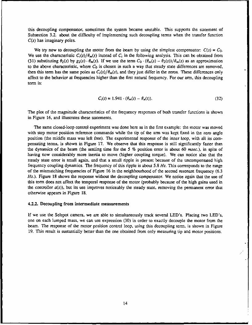
We try now to decoupling the motor from the beam by using the simplest compensator: C(s) = Co.We use the characteristic Ct(s)/Om(s) instead of C, in the following analysis. This can be obtained from(31) substituting 02(s) by g2(s) O m(S). If we use the term Co . (Om(s) - 02(S))/Om(s) as an approximationto the above characteristic, where Co is chosen in such a way that steady state differences are removed,then this term has the same poles as CI(s)/Om(s), and they just differ in the zeros. These differences onlyaffect to the behavior at frequencies higher than the first natural frequency. For our arm, this decouplingterm is:

C1(t) = 1.941 • (0m(t) - 0.(t)). (32)

The plot of the magnitude characteristics of the frequency responses of both transfer functions is shownin Figure 16, and illustrates these statements.

The same closed-loop control experiment was done here as in the first example: the motor was movedwith step motor position reference commands while the tip of the arm was kept fixed in the zero angleposition (the middle mass was left free). The experimental response of the inner loop, with all its com-pensating terms, is shown in Figure 17. We observe that this response is still significantly faster thanthe dynamics of the beam (the settling time for the 5 % position error is about 60 msec.), in spite ofhaving now considerably more inertia to move (higher coupling torque). We can notice also that thesteady state error is small again, and that a small ripple is present because of the uncompensated highfrequency coupling dynamics. The frequency of this ripple is about 5.8 Hz. This corresponds to the rangeof the mismatching frequencies of Figure 16 in the neighbourhood of the second resonant frequency (6.3Hz.). Figure 18 shows the response without the decoupling compensator. We notice again that the use ofthis term does not affect the temporal response of the motor (probably because of the high gains used inthe controller a(z)), but its use improves noticeably the steady state, removing the permanent error thatotherwise appears in Figure 18.

4.2.2. Decoupling from intermediate measurements

If we use the Selspot camera, we are able to simultaneously track several LED's. Placing two LED's,one on each lumped mass, we can use expression (30) in order to exactly decouple the motor from thebeam. The response of the motor position control loop, using this decoupling term, is shown in Figure19. This result is sustantially better than the one obtained from only measuring tip and motor positions.

14

5. Tip Position Control Loop

5.1. General Scheme

5.1.1. Basic Concepts

This section studies the control of the tip position. Sections 2 to 4 showed that the use of adequatecompensators and high gain controllers in the inner loop allows us to remove the effects of the friction.Once this has been achieved, the inner loop may be represented, for tip position control purposes, as alinear system of constant coefficients whose input is the desired angle of the motor 0,,,, and the output isthe actual angle of the motor 0re.

Another important result attained by closing the inner loop is that, because high gains are used in themotor position controller, the response of this inner loop may be quite fast compared with the dynamicsof the mechanical beam. This means that we can assume in many cases that this inner loop may berepreseLr..d by a unity transfer function. This is especially true in lightweight flexible arms. When thereaction torque of the flexible arm is important compared with the motor input torque then this assumptionno longer remains true. But it still may be used as an approximation in the design of the tip positioncontrol loop, and correction terms may be added later in order to compensate for the delays that appearin the response of the servocontrolled motor.

Assuming the previous statement, the only dynamics to take into account are those of the beamsubmodel, which are given by the transfer function g,,(s) of Figure 1. This transfer function relates theangle of the motor (input) with the tip position (output). This assumption allows us greatly simplify thedesign of the tip controller and to relate in an easy way the commanded trajectories with the mechanicallimitations of the beam, as the maximum stress in the structure for example. These two facts suggest thatthe two nested closed loops scheme here proposed is of general interest, and may be useful even in thecase where the friction in the joints is not important.

Several approaches may be used to control the tip position, either from state space or frequency domaintechniques, or either using feedback or feedforward controllers.

Feedforward terms have been often used in the control of rigid arms : Craig [ 14], Khosla and Kanade[15] a.e. The feedforward term generates, in these schemes, a torque (current) to drive the arm thatis function of the desired trajectory. The feedback control loop compensates for the tracking errorsproduced by perturbations. Feedforward functions may be generated off-line previous to the motion, butit is desirable to be able to generate them in real time in order to face unexpected changes in the trajectoryas for example happens in robots with sensors. Feedforward functions have been used to drive flexiblestructures without exciting the resonant modes (Meckl and Seering [161 a.e.), but they are complex anddifficult to use for real time control, especially when several resonant modes have to be considered.

The other approach is the design of feedback controllers to actively damp the vibrations producedwhen moving these flexible structures. Several methods have been proposed and experimental results areavailable. Examples are Cannon et al. [1], Matsuno et al. [2] and, recently Kotnick et al. [17] . Mostof these methods are based on state space techniques. They use optimal control and normally need toreconstruct from tip and motor measurements some states of the system by using observers or filters.

A simple general scheme is proposed here that combines a feedforward term with a feedback controller.Three different feedback schemes are described here. It is shown that, with our simple scheme, high

15

positioning performances may be achieved for the tip o: a flexible arm. In this scheme, the feedforwardterm is mainly responsible for driving the motor in such a way that the tip of the arm follows thedesired trajectory. The closed-loop controller compensates for the deviations of the tip from the nominaltrajectory. If the feedforward term is properly designed, these errors will be small allowig us to use verysimple controllers to compensate for them.

The feedforward term is studied in Subsection 5.2 neglecting dynamics of the inner loop. A correc-tion term is also proposed in this subsection to take into account the dynamics of this loop. Feedbackcontrollers are described in Subsection 5.3.

5.1.2. Error Analysis

The scheme proposed here combines a feedforward term very simple to generate, with a simple feedbackcontroller. We show that we can get controls that provide high dynamic performance by using some sim-ple rules from the classical frequency domain control methods. Combined feedforward/feedback controlschemes have been used before for flexible structures, as for example Dougherty et al. [18], that usedacceleration feedforward in the pointing control of the Space Telescope, or recently Gebler [19], that usedan approximate feedforward term to control a two degree of freedom flexible arm. Our feedforward termdiffers in that it uses motor angle rather than torque as the generated signal. Thus the feedforward termmay be defined as the inverse of the dynamics of the beam (in the minimum phase case). This term issimpler than the terms generated in the above mentioned methods, and can be easily computed in realtime.

Figure 20 represents this scheme. We have included in the arm model two kinds of perturbations, onein the angle of the motor and other in the angle of the tip. The first one (bl (s)) models residual errors inthe positioning of the motor because of the Coulomb friction, residual errors in modelling the dynamics ofthe motor (because of changes in the dynamic friction for example), errors because of the assumption thatthe transfer function of the inner loop is equal to one, and even errors because of unexpected permanentbending in the beam. The worst errors are those due to the Coulomb friction and the permanent bendingof the beam because they cause steady state errors. This is modelled by a step input: 61 (s) = 61 Is. Thesecond perturbation (62(s)) models deviations of the tip from the desired trajectory because of externaldisturbances. Perturbation 62(s) is modelled in this case by a polynomial in s because it is a transienterror. Finally, notice that in Figure 20, gn(s) = g,,(s)/gM(s).

5.1.2.1. Discretization.

The system of Figure 20 is a hybrid system in the sense that it has analog and discrete components.In order to simplify the design, a discretization of the analog blocks is done, and a digital controller inthe z - plane is designed. The discretization is done using the residues formula for continuous-discreteequivalent sampled systems with generalized holds (Feliu [201, e.g.):

G(z) = X (z'). Z [G(s) • X2(s)/X 3(s)I, (33)

where G(s) is the transfer function of the continuous plant, and X 1, X 2 and X3 are polynomials thatcharacterize the hold and its interpolation properties.

This way of discretization is preferred to others (Tustin transform for example) because it gives anexact matching between the discrete and analogical signals at sampling instants (VanLandingham [21],

16

e.g.).

The following assumption is made: if we sample the angle of the motor 0, with period T, then thissignal may be approximately reconstructed from its samples by interpolating between the samples bystraight lines. It can be shown that it is equivalent to reconstruct the signal from its samples using a firstorder non-causal hold. In this case:

X(z - 1) = z. (1 - z-) 2 , X2(s) = lT, X 3(s) = s2, (34)

and g,,(z) is obtained from (33) using this hold and making G(s) = g,,(s). Transfer function A(z) is the

sampled-data equivalent transfer function of the motor ih(s) after having removed the Coulomb friction

and the beam-motor coupling by using compensating terms. A zero order hold is used to obtain thisdiscrete transfer function from expression (33). Now G(s) = in(s), and:

Xt(z - 1) = 1 - z 1 , X2 (s) = 1, X3(s) = s. (35)

The partial scheme of Figure 21, that does not include the perturbations, illustrates this discretizationprocess. The scheme of Figure 22 is obtained where:

,M(z) = a(z) .A(z) (36)1 + a(z) . b(z). th(z)"

It can be easily shown that the two mentioned perturbations may be grouped for control purposes in aunique perturbation 6(z) (Fig. 22). It is now of the form:

6(z) = )"(1 ) (37)

6,, being a polynomial in z- 1 , and g,,d(z- 1) the denominator of g,,(z). The factor I - z- 1 of the denominatoris produced by the pole in the origin of perturbation 61, and numerator 6, is a combination of bothperturbations b, and b2.

The only approximation made for deriving Figure 22 is the mentioned interpolation. Transfer functionsh5(z) and M(z) are exact in the sense that they model exactly the behavior of the motor and inner loopat sampling instants because the input to the motor comes from a D/A converter and it is adequatelymodelled by a zero order hold.

5.1.2.2. Analysis.

From the block diagram of Figure 22 we get:

O(z) = M(z) . g,,(z) " (R(z) + N(z)) (38)

O9r(Z) I + M(z) . g,.(z) " R(z)

O,(z) 1

6(z) 1 + M(z) . g,,(z) . R(z) (39)

17

If the feedforward term is of the form:

N(z) = g-' I (z) .M-' (z) . U(z), (40)

then the error in O due to the reference trajectory (assuming no perturbations) is:

1 - U(z)eo,,(z) = 1 + M(z) . gn,(z) - R(z) Or(Z). (41)

The error due to the perturbations is, combining (37) and (39):

-(1 -z-)e6 (z) = .(VndZ) (I--))(42)1 + M(z). gn(z). R(z)

The steady state error analysis indicates that it is necessary to use a controller with integral feedback toeliminate steady state errors. So, it suggests that R(z) should be a P.I.D. controller.

5.2. Open-Loop Control

Expression (41) gives a very straightforward criterion for choosing the feedforward term: the closerU(z) is to 1, the less eo,,(z) is. Ideally, we just need to make U(z) equal to 1 to get a zero tracking error.U(z) = I means that the feedforward term does the perfect inversion of the dynamics of the arm whichis expressed as a relation between the commanded angle for the motor and the angle of the tip. But,unfortunately, it is not possible to do this in many cases when trying to control flexible arms. There arethree causes that preclude the use of the perfect inversion of the system as a feedforward:

1. Transfer function gn(s) (or gn(z)) is normally non-minimum phase. It means that this transferfunction has zeros in the right half-plane. When inverting it, the feedforward term becomes unstableproducing unbounded control signals.

2. Transfer function M(z) is non-minimum phase or has zeros such that their real component is negative.The same as above applies here when M(z) is non-minimum phase. In the other case, the invertedterm remains stable but the feedforward control signal generated is extremely oscillatory.

3. Delays in M(z). When inverting it, the feedforward term becomes noncausal. If the feedforwardcontrol signal is precomputed, it is not a problem. But it impedes the real time generation of thissignal. It is important to mention that gn(z) does not present this problem because it was calculatedusing a non causal hold.

Notice that the first problem is related to the inversion of the dynamics of gn(s), and the other two tothe inversion of the dynamics of the inner loop. So, if the inner loop is much faster than the dynamics ofthe beam, we can assume that M(z) = I and we just have to face the first problem. Subsubsection 5.2.1. isdevoted to the study of this simplified case. The profile of the tip trajectory is deduced in Subsubsection5.2.2., assuming this simplified case. The general case, where thL, dynamics of the inner loop are includedin the feedforward term, is studied in Subsubsection 5.2.3.

18

5.2.1. Feedforward term

An original method is proposed here that allows us to generalize the use of the inverse dynamics feed-forward term to non-minimum phase systems. It will be seen that in this case an approximate inversedynamics term is generated that minimizes the differences between the desired and actual behavior of thetip of the arm.

Let us assume a stable system whose transfer function is g(s). Assume that we want its output tofollow a nominal trajectory, represented by its Laplace transform u(s), as close as possible minimizingthe ISE error (integral squared error):

ISE f e(t)_dt_ f "cOISE= 2 (t). dt e(s) -e(-s) -ds. (43)

Then the feedforward term (see Figure 23) that optimizes this with the constraint of being stable is givenby the expression:

g.(-S).tUUS)]

US) = g.(s).+Iu(s) (44)

where:

gn(s), gn(-s) = g+(s), g (s),

g+(s) groups all the poles and zeros of g,(s) • gn(-s) that are in the left half-plane, and g-(s) all whichare in the right half-plane;

Iuu(s) = u(s) .u(-s) = J+u(S) .IUU(s),

where again 1 >uu(S) groups all the poles and zeros of Iuu(s) in the left half-plane and 13U(s) all which arein the right half-plane; and

gn(-s). Iuu(s) [g.(-s) Iuu(s)1 + [gn(-s). Iuu(s)1g -(s) u(S) L ; J + L g;_ (S) - 'UU(S)

where, assuming that the partial fraction expansion of the left hand member of the above equation hasbeen done, the + term represents the grouping of the fractions corresponding to the roots placed in theleft half-plane and the - term represents the grouping of the ones corresponding to the roots in the righthalf-plane.

This method is just a slighi modification for open-loop control of the technique to obtain optimalcontrollers described and demonstrated in Gupta and Hasdorff [221. Notice that we are minimizing a costof the form

19

J - 0j [u(s) (1 - ,,(s). g.(s))]. [u(-s) •(1 - g,(-s))] • ds,j.00

therefore if gn(s) is minimum phase, then k,,(s) = g-l(s) and, as consequence of all this, the continuousfeedforward term in this simplified case will be of the form

N(s) =

This method allows us to design an analog feedforward term that nearly cancels (if non-minimumphase system) or completely cancels (if minimum phase) the dynamics of gn(s). If we denote the desiredtrajectory for the tip position as Pp, the tip will not follow exactly this reference in the non-minimumcase. Instead, it will follow a new reference profile 0,, obtained from passing Pp through a filter whosetransfer function can be easily seen that is g,(s) -,(s). Then:

0,.(s) = gn(s). (s) . PP(s). (45)

In the minimum phase case, this filter will be 1. The property of this filter, according to (43), is thatthe new reference trajectory 0,,(t) is as close as possible to the desired reference Pp(t), but taking intoaccount the constraint of a bounded 0,,.

Finally, we have to mention that, in the scheme of Figure 22, the feedforward term is discrete. Thisterm is implemented by generating the signal 1(t) of Figure 23 and sampling it with period T to producethe sequence i(k) used in the control as it is shown in Figure 24. A discrete version of formula (44) alsoexists that directly gives a discrete feedforward term g,(z). We preferred to use the continuous veronand then sample the output because it is easier to compute and because the use of the discrete versioncan easily produce feedforward terms with the problem stated above of having stable poles with negativereal component, generating a high frequency oscillatory control signal.

It will be stated in the next subsubsection that the nominal trajectories used in this work for the tipposition are second order parabolas. It can be easily shown that, for this class of trajectories, i(k) may begenerated from the samples of the nominal trajectory O,,(k) passing this sequence through a block N(z)(see Fig. 22) whose transfer function is:

- ) [ = N(z) (46)ST2 .z . (l+z - ) s3

5.2.2. Trajectories

Most of the work done on closed-loop control of flexible arms is based on the use of step functionsas command signals because they are easy to generate, and the responses of the arm to such inputs maybe easily analyzed. But the command signals typically utilized in existing industrial and research robotsare parabolic trajectories of order at least two. This is because the desired trajectories for a robot needto have bounded derivatives until at least the second order, in order to take into account the mechanicallimitations of the arm. In fact, the second derivative of the trajectory is its acceleration, whose value

20

is bounded by the maximum torque permissible in the mechanical structure and, in some castes, by themaximum current allowed in the motor.

These considerations are also important in flexible arms. If the purpose of a flexible arm is to carry aload at a high speed using a lightweight arm, the acceleration must be limited to prevent excesive bendingin the structure that could damage it.

Further, it is apparent that relaxing the sharpness of the trajectory allows the arm to follow thetrajectory better, avoiding in some cases undesired movements (overshooting) that may be producedusing step inputs, and avoiding excessive control signals that can saturate the amplifiers. For example,Cannon et al. [1] reported this beneficial effect in the control of flexible arms when rounding the comersof the steps.

In the opposite sense, sophisticated trajectories have been used to open-loop drive flexible structures.Different optimization criteria have been used that take into account the limitations of the mechanicalstructure: Farrenkopf [23], Turner and Junkins [24] or Meckl and Seering [16], a.e. The generationof trajectories using these techniques is computationally laborious making them not suitable for on-linecontrol of flexible arms with several yibrating modes, when computer capacity is limited.

In this subsection we propose a family of trajectories that compromise the above considerations. Theymust be simple enough to be generated in real time (and to allow a real time generation of the feedforwardcontrol signal), but they must take into account the physical limitations of the mechanical structure. Thesimplest trajectories that fulfill this are the parabolic trajectories. For this reason they are usually utilizedin rigid arms. We are going to show here that they can also be utilized for minimum phase flexible arms,but not for non-minimum phase flexible arms because the feedforward signal cannot be generated in thiscase. We propose here a family of trajectories for this last case. We call them quasi-parabolic trajectories.

These trajectories are represented in Figure 25. They are characterized by the fact of being verysimilar to the parabolic trajectories, but having bounded derivatives up to forth order. The accelerationprofile of the quasi-parabolic trajectory is the same as the parabolic trajectory with a slight rounding inthe comers. So, the quasi-parabolic trajectory behaves most of the time as a parabolic trajectory. Only invery small intervals of time, that conespond to !he :t-L'oes in *= : zclzration, both trajectories behavedifferently.

5.2.2.1. Choosing the trajectory

Here we give a criterion for choosing between the two trajectories described in Figure 25. We willalso justify the necessity of the quasi-parabolic trajectories.

In order to calculate the feedforward term, we assume in expression (44) that the nominal trajectoryis a parabola whose Laplace transform is u(s) = 2/s 3. Taking this into account and operating (44) we getthe general expression used in this paper to calculate the feedforward term:

s 3 g g(- s) Ig,.(s) = -_s) g (s) s3 J (47)

and assuming that g,(s) is of the form:

21

rJ(S - a,). l-I( -g.(s) = RK. i=1 j=1

d(s)

where ai < 0, 1 < i < n1; bj > 0, 1 < i n2, and all the roots of d(s) are in the left half-plane, operatingwe obtain that:

d(s). (a2" S2 + 011 • S + a0)

Ws) =2 (48)x. I(S - ca,). II(s + ji=1 j= 1

Rt2

fJ(s + bj)where the a coefficients are obtained from the partial fraction expansion of j_- aO..a2

,3 fl(s -b)j=1

being the coefficients corresponding to the terms whose denominators are s, S2, S3 respectively The filterof expression (45) is then

n2

1l(s- bj)gn(s)" -N(S) = (a2 S2 + al • s + a0) - =1 (49)

l1 (s + bj)J=1

and the following lemma is deduced, that justifies the necessity of the quasi-parabolic trajectories.

Lemma 1:

Assume we want to control a flexible arm using parabolic or nearly parabolic commands, and wewant to use a feedforward term to drive the arm. Then, with the exception of rare degenerate cases,the order of the numerator of the feedforward term k.(s), calculated from (47), may exceed the orderof the denominator by a value of 2 if gn(s) is minimum phase, or by a maximum value of 4 if ga(s) isnon-minimum phase.

This lemma is easily proven using equation (48). If the system is minimum phase, then a2 = a1 = 0.If it is non-minimum phase, in general these coefficients will be nonzero. We denote the order of thispolynomial as na,. Moreover, the difference between the order of the denominator of g,(s) and the orderof its numerator is 2 because of the form of the dynamic model of the beam (see equation (13) of Part IReport), with the exception of the rare cases in which the n element of vert': 6 is 0. Then we find thatthe difference between the order of the numerator and denominator of ,(s) is n, + 2 which is always lessthan or equal to 4.

If the system is minimum phase then this number is 2. If it is non-minimum phase, may be up to 4,and the lemma is proven.

Notice that the feedforward term may then be expressed as

22

9.(S) =" gn4 " S

4 4 +gk3 " S3 +" N2 " S2 +t gn I + -k ,O + gap(S), (50)

wlere kno,... , g4 are constants that may take the 0 value, and gp(s) is a proper rational function in s.Notice also that, as result of this, the difference between the orders of the numerator and denominatorof k,,(s) gives the order of the maximum derivative of the nominal trajectory needed to generate thefeedforward signal, and that consequently has to be bounded. From this and the previous lemma itfollows that parabolas (bounded up to the second derivative) can be used for minimum phase systems,but normally cannot be used for non-minimum phase systems. Quasi-parabolic trajectories with derivativesbounded up to the fourth order may be used in these cases.

Finally, when we use quasi-parabolic trajectories, the feedforward term of expression (47) is just anapproximation (it was obtained for a parabolic reference). But because of the closeness between thesetwo kinds of trajectories, this approximation is normally sufficient.

5.2.2.2. Designing the parameters of the trajectory

The parameters of the trajectory: maximum acceleration and second derivative of the acceleration, maybe designed approximately from expression (50), taking into account the physical limitations of the me-chanical structure. In general, these limitations may be expressed in terms of the coupling torque betweenthe beam and the motor, which may be expressed as a function of the beam deflection:

C1(s) = C(s) deflection(s), k5 1)

where C(s) is scalar for massless beam case.

This deflection may then be expressed as

deflection(s) = [9 4 g •S3 + kn2 S2 + gnl • S + (9,0 - 1) + gnp(s)l - 01r(s) (52)

and, in many cases, the deflection may be kept between the safe boundaries just by choosing an appropiatevalue for the maximum derivative of 0nr, needed to compute the above expression. This will be illustratedwith examples.

For massless beam, stresses at all points will be proportional to deflection. So torque limit is propor-tional to deflection.

Another physical limitation is the maximum current allowable in the motor. Conditions for the deriva-tives of the trajectory may be obtained from (50) in conjunction with the model of the motor. But theyare normally quite more complex than the conditions derived from (52) for the deflection. Moreover, inour two flexible arms, the above developed mechanical condition is more restrictive than the one obtainedfrom the motor current limit, making unnecessary the consideration of this last constraint.

5.2.3. Considering inner loop dynamics

We mentioned before that, if the inner loop is fast enough compared with the outer loop, then M(:) = I.In this case, problems 2) and 3) described in the beginning of Subsection 5.2. do not exist, the procedure

23

described in Subsubsection 5.2. 1. applies, and the feedforward term is significantly simplified. It willbe seen in the experiments of the next section that this assumption is very often true when controllinglightweight arms, although there are cases in which the dynamics of the inner loop must be taken intoaccount. In these cases, the problems caused by the non-minimum phase zeros of M(z) may be overcomeby using the discrete version of the method described in the previous section. But the oscillations causedby the inversion of the zeros that have a negative real component cannot be removed. In order to avoidboth kinds of problems as well as the above stated noncausality problem, an optimization method withconstraints is proposed.

Assume the system has n, zeros in th. situations described in the case 2). Let us call them pi. Assumealso there are D delays in M(z) (D pole3 in the origin). Then a feedforward term of the following formmay be used:

NWz= (z').M()[nl ' = i Z "zD'f(z)=g'lI(z)'M-(z)'U(z)' (53)1i - 'oi

where k,(z- 1 ) = kn,(z- 1 )/d,,(z - 1' is the term calculated in Subsubsectior, 5.2.1. from gn(s), gn(z- 1 ) =

g,,(z-')/g,(z-'), and f(z) =f,(z)/fd(z) is a correction term whose calc,:1ation is the objective of thissubsubsection.

It has been mentioned that trajectories based on second order parabolas are used here. It seemsdesiderable to make the arm follow these parabolas without steady state error. In order to guarantee this,it can be easily seen from equation (41) that the following condition must be fulfilled:

I - U(z) = (1 - z-) 2 . W(z), (54)

W being a rational function in z. Combining this with equation (53) we get:

1-I(1-oi).-,,,a(z-l).-gnd(z-').'fa(z)-I - oi - ).- ° .,(z-t).g gn(z-').fn (z) = z(- z-t).(z), (55)

where W,(z) is a polynomial. Transfer function f(z) may be calculated in such a way that the trackingerror is minimized. Again we propose to minimize the integral squared error of (41):

00

Cost = e 2 (k).k=O

But now, apart from the stability condition as given in Subsubsection 5.2.1., the following constraintsshould be also fulfilled by the feedforward term:

* Zero steady state tracking error of a parabola (equation (55)).

e No stable poles in the left half plane.

@ It must be a causal term (no zeros in the origin). This condition is optional, depending on if a realtime feedforward term is wanted or not.

24

A numerical method is proposed to calculate the optimum f(z) that accomplishes all these conditions.Previous to its calculation, the form of f(z) should be defined (orders of numerator and denominator).This is given by the following lemma.

Lemma 2:

Assume that the difference between the orders of the numerator and denominator of k,(z- 1 ) • gn(z - ' )

is v, n. is the number of zeros causing problem 2), and D is the number of delays of M(z). Then theminimum order of the denominator of f(z) that accomplishes the above optimization constraints is given(exceptuating degeneracies) by:

order fd(z) = n, + D + v + 1 (56)

and the order of the numerator is

order f(z) = 1. (57)

This lemma may be easily proved taking into account that the accomplishment of the constraintsimplies that a number of order fd(z) parameters must be tuned to make f(z) stable, plus two parametersmore in order to make I - U(z) have two zeros at 1 (null tracking error condition).

Knowing the order of the f(z) transfer function, its coefficients can be chosen in such a way to op-timize the above defined cost. Some of the existing numerical search methods may be used to get theoptimum parameters of f(z).

5.3. Closed-loop control

5.3.1. Classical control using tip position feedback

The use of a controller with an integral term is proposed, in order to remove permanent errors (Fig.26). We mentioned before that the use of a feedforward term allows us to simplify this controller. Often,simple PID controllers may be used to get good positioning performances. Moreover, the examples willshow that if a perfect compensation of Coulomb friction is provided, the feedback controller may even besimpler because the integral action is not needed. All this allows us to use high sampling rates improvingthe general behavior of the digital control system.

These controllers may be easily designed using, for example, classical frequency domain techniques.The function of this controller is to compensate for the deviation of the tip position from the desiredtrajectory. To move the arm to the desired angle, most of the control action required is provided by thefeedforward term. When the arm is not moving and a deviation from the -.ference position is producedby an external disturbance, the control action to recover the desired position is provided by the controllerR(z). The fact that this controller compensates for only small deviations allows us to use high gains (whenthe system is minimum phase) without saturating the amplifier of the motor. This produces a significantimprovement in the dynamic performances of the controlled system.

25

5.3.2. Control that cancels the first natural frequency by using tip position feedback

This scheme is composed of two loops: a loop that cancels the first natural frequency, and a classi-cal P.D. controller with a feedforward term as shown in Figure 27. The control components are designedin three steps:

1. A positive unity feedback loop is closed to remove the first vibrational mode. This loop alwaysremoves the first vibrational mode because g.(O) = 1 in all flexible arms.

2. A compensator is designed that cancels the poles of the remaining system, and its minimum phasezeros.

3. A P.D. controller is designed (in the case of a single non-minimum phase zero) with a feedforwardterm. In the case of more than one non-minimum phase zeros, a controller designed using thestandard pole assignment technique may be used, instead of the P.D. controller.

The feedforward term is designed here using the procedure described in Subsection 5.2., but takinginto account that now the g,(s) transfer function that has to be used is the resulting from steps I and 2of the above described method.

5.3.3. Control using feedback of position at several points of the beam

The general scheme of this controller is also composed of two terms: the feedforward term discussed inSubsection 5.2., and a feedback controller that uses the measurements of positions at intermediate pointsof the beam.

Feedback controllers may be designed using any of the standard control design methods. Good resultsare achieved using optimization techniques ([25], e.g.) to design a controller: y(s) = -A . x(t) that drivesx from an initial state to the zero state minimizing a cost function of the form:

. (xT(t) • R, -x(t) + R2 - t (58)

where R 1 E R2"nx2 "n,R2 E R are weighting matrices, and x E R2n is the state vector of the system. Fromequation (13) of Part I, and making T, = F, = 0, we get the state equation of the system:

it)0 I. .xWt + ,,0 - OMWt (59)(t= E.I.M-1 -A 0 E.-I. .I1

A B

where xT(t) ( 6 T7 ), and &n E R"'XA is the identity matrix. This model is simpler than modelsused in other approaches (that relate 0,(t) and Om(t) with i(t)), producing simpler controllers.

If there were dynamic friction in the tip, then F would be proportional to the speed of the tip massand a coefficient would appear in the position (2 • n. 2 • n) of matrix A of the before equation.

26

This feedback scheme uses the errors between the desired and the actual states to generate the control

signal. Defining A = ( At A 2 ); Ai, A2 E R-1 we can express the control signal (y) as a function

of the measured variables: 7(s) (A, + A2 . s). (O,(S) - e(s)).

The reference vector for the measured variables ((9,) may be obtained from the reference 0, by usingthe following expression:

(9,(S) = T(s) . O,, (60)

C1 • Adj(M -$2 - E . I.A). E .1 13

C2.Adj(M s2 - E .I.A).E..3 I (61)

s=Cn.Adj(M s2 - E .1.A). E..3 (61)

Cn.Adj(M S2 - E.1. A). E .13

where Ci = (0 ... 0 1 0 ... 0) the I being in the i - th column. These last equations are

obtained from equation (16) of Part I. Logically T = I results.

In the case of a non-minimum phase system, the denominator of T has some positive real componentroots. But they are cancelled with the zeros of filter (49), leaving (9,(t) bounded. Cancellation may beexactly done because all these terms are computed.

This feedback control scheme presents important advantages over other existing schemes when im-plementing it with a digital computer. Other control methods need to reconstruct the whole state x frommeasurements of the motor and tip of the arm by means of filters or observers. They involve a largeamount of computation. In many cases, these reconstructions are distorted by the noise of the measuredsignals making the control difficult. But in our case, because a) we have simplified the arm dynamicsby clos'ng the motor position loop, and b) we are using more sensing in the beam, all the states maybe easily obtained: positions are measured and velocities may be approximated by the simple differenceequation O(k. T) = (0(k. 7) - 9((k - 1) • T))/T where T is the sampling period and k is an integer.Because only the first derivative of measured signals is needed, this approximation of the velocities ofthe mass points is reasonable in many cases, even having relatively high levels of measurement noise.

Figure 28 shows the details of this control scheme. Notice that first derivatives of the position errorsignals are used instead of first derivatives of the position states.

5.33.1. Influence of the payload

We study in this subsection how changes in the payload affect the dynamics of the controlled sys-tem.

Inner loop

The motor position control loop is not directly affected by changes in the payload. Payload influences thedynamics of this loop only through the coupling torque between the motor and the beam. This coupling isbeing compensated by using expression (15) to estimate the coupling torque from position measurements.Coefficients hi are independent of the payload and consequently no term of the inner loop needs to betuned as a function of die payload.

27

Payload affects this loop indirectly if we consider the saturation limits of the motor current. If thepayload is too high, the current saturates and control performance deteriorates. But for the normal rangeof payloads, performance of this inner loop may be considered invariant.

Feedforward term

Because of the Zero Invariancy Property described in Part I, the filter expressed in (49) is indepen-dent on the load, and variations in the feedforward term (48) are due only to the factor d(s)/K. So k^(s)can be easily tuned to payload changes by changing only one parameter in its numerator as it will beillustrated in the example.

Feedback term

The gain factor and poles of the closed-loop transfer functions matrix 9 (((s) = 9(s) • er(s)) changewith the payload. But zeros of the transfer functions gt,i; I < i < n of the last row of this matrix remainconstant. Notice that these transfer functions characterize the closed-loop dynamic behavior of the tip ofthe arm.

Proof of zeros invariancy: the closed-loop state equation (without the feedforward term) is:

x(t) =- S.Aj) -E.I.M-.B.A 2 ) + ( E.I.M-.13.A1 E.I.M-S.B.A 2

e( W (In 0 ).x(t),

where x7 is the state reference; and operating:

0(s) = (s2 -M + s - .E . . A2 + E. I. (-A + B. A,)) - ' ,. .3. (Al + s. A2). Or(s).

In this expression, 9(s) shows the same dependence of M as expression (16) of Part I. Then, thesame reasoning that supports the Zeros Invariancy Property is applied here to demonstrate this.

Finally, only numerators of 2 are affected by changes in the payload. Their dependence on m, issimilar to the dependence of kn(s).

6. Tip Control Experimental Results

Control methods described in this report are applied here to our two flexible arms, whose dynamicswere modelled in Part I. Experimental results are shown.

28

6.1. Single-mass flexible arm

6.1.1. Discretization

This system has only one vibrational mode and it is minimum phase. The transfer function of thebeam was found to be (see Part I):

43.75s2 + 0.06 s + 43.75 (62)

Applying the discretization method suggested in Subsubsection 5.1.2.1. we get:

gi(z) = 0.6583. o10- - I + 3.984848485. z- I + z - 21 - 1.999423 • z- 1 + 0.999817 • z- 2 (63)

And the sampled data equivalent transfer function of the inner loop is

0.0309247. z-2 (1 + 0.857737056 • z- ' - 0.139691015. z- 2)1 - 1.993393 • z- '+ 1.199567748 - z- 2 + 0.00159364 • z- 3 - 0.179119249. z- 4 +0.0244809 •- 5

(64)

We can notice that M(z) has a delay D = 2, and a zero in -0.99774394.

6.1.2. Open-loop control

6.1.2.1. Simplified feedforward term

The settling time to a step input of the inner loop was found to be 30 msec. So it is much fasterthan the dynamics of the beam and it may be assumed that M(z) = 1.

Because gl(s) is minimum phase, we get from (48) that kl(s) = g- 1(s). And because of the assumptionM(z) = 1, we have that the feedforward signal 1(k) is given directly by sampling the output of ti(s).

Because the system is minimum phase we use the parabolic trajectory to command the arm. The onlyparameter to calculate there is the maximum acceleration and this can be easily obtained from equation(50), taking into account that in this case C(s) of expression (51) is a constant. It means that the torqueis directly proportional to the deflection. The maximum allowed deflection for this beam is 400 mrad.(23 degrees). Using equation (50) we get the simple expression:

deflection = acceleration/43.75, (65)

and, therefore, the maximum acceleration is 8750 mrad/sec2 . We have assumed a deflection of 200 mrad.

29

(50 % of the maximum deflection) to calculate this acceleration, in order to allow some extra deflection

for the action of the c, atroller R(z). Figure 29 shows the resulting feedforward signal.

6.1.2.2. Complete feedforward term

Because there is a zero of M(z) in the left half-plane (n, = 1), and a delay of two sampling periods(D = 2), the inverse of M(z) cannot be directly used for a real time feedforward compensation of itsdynamics. In the experiments carried out here, the feedforward term is precomputed so, the delays arenot a problem. Ih order to cancel the effects of the left half-plane zero in -0.997744 then, according toSubsubsection 5.2.3., M-1 (z) is multiplied by the factor (1 + 0.997744 . z-1 )/1.997744. And a correctivef(z) term is calculated taking into account the conditions stated in those subsubsection:

f(z) = 1.20912 - 0.870105 z-

1 - 0.661 • z-1

Notice that, according to Lemma 2, the order of the denominator should have been 2. This is adegenerate case where the coefficient corresponding to z- 2 is 0. Figure 30 shows the implementationscheme of this feedforward term, and Figure 31 shows the feedforward signal generated.

From comparing Figures 29 and 31 we see that both feedforward signals are quite similar. The onlysignificant difference is given by some impulses produced at the instants when the value of the acceler-ation changes. These impulses tend to speed up the motor in these changes, in order to compensate thedynamics of M(z). Experiments showed that including the dynamics of M(z) in the feedforward term didnot produce any significant improvement in the control of this arm. So in what follows, we will use thesimplified feedforward signal shown in Figure 29.

6.1.3. Closed-loop control using the first scheme

The first scheme coincides with the third one in the case of a single-mass flexible arm.

R(z) was chosen to be a simple digital P.I.D. controller and was obtained by minimizing the timeneeded by the arm to recover its desired position when changes in the position were produced becauseof external perturbations. The perturbation model represented by equation (37) was used. We assumedthat we had a combination of two perturbations : a permanent error position perturbation in the angle ofthe motor, and a perturbation on the tip because of erroneous initial conditions. The resulting optimumcontroller was

= 100. (1 -0.98. z-). (1 -0.99. z- 1)(I - z-1) •-(I - 0.61 -z- 1)

Figure 32 shows the tip response of the parabolic profile. It shows that the arm slightly leads thereference because of the feedforward term. The settling time is of 0.22 sec. A comparison between theangle of the tip and the angle of the motor is given in Figure 33, showing that the dynamics of the innerloop is very much faster than the outer loop, and the movements required are larger.

30

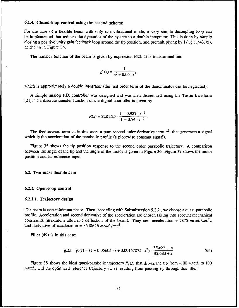
6.1.4. Closed-loop control using the second scheme

For the case of a flexible beam with only one vibrational mode, a very simple decoupling loop canbe implemented that reduces the dynamics of the system to a double integrator. This is done by simplyclosing a positive unity gain feedback loop around the tip position, and premultiplying by 1/w2 (1/43.75),cz!' , .-i in Figure 34.

The transfer function of the beam is given by expression (62). It is transformed into

1s2 +0.06. s'

which is approximately a double integrator (the first order term of the denominator can be neglected).

A simple analog P.D. controller was designed and was then discretized using the Tustin transform[21]. The discrete transfer function of the digital controller is given by

1 - 0.987*•z-1R(z) = 3281.25 -0.74z

1

1- 0.74.-z- 1

The feedforward term is, in this case, a pure second order derivative term s2, that generates a signalwhich is the acceleration of the parabolic profile (a piecewise constant signal).

Figure 35 shows the tip position response to the second order parabolic trajectory. A comparisonbetween the angle of the tip and the angle of the motor is given in Figure 36. Figure 37 shows the motorposition and its reference input.

6.2. Two-mass flexible arm

6.2.1. Open-loop control

6.2.1.1. Trajectory design

The beam is non-minimum phase. Then, according with Subsubsection 5.2.2., we choose a quasi-parabolicprofile. Acceleration and second derivative of the acceleration are chosen taking into account mechanicalconstraints (maximum allowable deflection of the beam). They are: acceleration = 7875 mrad./sec2 .,2nd derivative of acceleration = 8648646 mrad./sec4 ..

Filter (49) is in this case:

g,(s) . b(s) = (1 + 0.05605 • s + 0.00157075. s2 35.683 - s (66)35.683 +s

Figure 38 shows the ideal quasi-parabolic trajectory Pp(s) that drives the tip from -100 mrad. to 100mrad., and the optimized reference trajectory On,(s) resulting from passing Pp through this filter.

31

6.2.1.2. Feedforward term

It is given by expression (48) (expressed in function of the payload m2):

(0.12136.m2.s4+(176.6032.m2+2.6791).s +852.81575). 14 0.05605 -s + 0.00157075 -s 2

0.6697676. (s + 35.68333)2

m2 appears only in the first factor. Then this feedforward term may be easily tuned as function of thepayload using the scheme shown in Figure 39. Particularizing to our example (m2 = 0.12136 Lb.):

g,,(s) = (s4 + 1637.1 • s 2 + 57903.3175). 1 + 0.05605 . s + 0.00 157075 s 2 (68)45.475 (s + 35.68333)2

6.2.2. Closed-loop control using the first scheme

In the inner loop, the motor was decoupled approximately from the beam by using expression (32).

The feedforward term expressed in (68) was implemented, and a digital P.D. controller was used whoseparameters were experimentally tuned. It was of the form

R(z) = 4.891 1 - 0.985111 - 0.94174 • z-

Figure 40 shows the tip response to the quasi-parabolic profile. Notice that the first vibrational modeis completely cancelled, and the second one is reduced to a small damped ripple (the amplitude of thelargest ripple is less than 3% of the step amplitude). The settling time is 0.3 sec. Figure 41 shows thecomparison between the angle of the motor and the angle of the tip, and Figure 42 shows the tip positioncontrol action provided by the feedforward term compared with the one provided by the controller R(z).Notice that the use of a P.I.D. controller has not been necessary because the effective compensation of theCoulomb friction and static coupling torque carried out in the inner loop removed the permanent errors.

A more complex controller could have been designed here in order to remove the remaining ripple,and include some integral action, as was suggested in Subsubsection 5.3.1. However, this has not beendone because the purpose of this example was to show that it is possible to control flexible arms of rela-tively complex dynamics with a simple feedback controller (in this case with a PD. controller) if a properfeedforward term is used. This feedforward term was shown to be easy to generate. Therefore, flexiblearms of complex dynamics may be controlled using control units of modest computing capabilities.

6.2.3. Closed-loop control using the second scheme

We use here the same method as in 6.2.2. to decouple the motor from the beam.

The transfer function of the two-mass flexible beam is:

32

-T. (s2 - Q2)

gM(s) = (s2 +.).(s 2 + .2 )

2 2

where w and W2 are the natural frequencts of the two vibration modes; and k = w • W2/ or.

The method to design the tip position controller is

1. Cancellation of the first (lowest frequency) vibration mode by closing the positive feedback:

-K . (s- - a,)gn'(S) =2+s2 . (s2 + W2 + W2+

2. Cancellation of the remaining minimum phase dynamics. We use a compensator of the form

52 + +W2 +/k

R . (s + az)

to reduce the dynamics of the beam to

g2(s) = a " (69)

3. Feedforward term. We apply expressions (48)-(49), but using g,(s) instead of g,(s). We get thatthe feedforward term of scheme of Figure 34 is of the form:

- . (1 +--.S+--. s2 )

$ + z az a2

It is easy to prove that the filter of expression (49) is the same in all three methods.

4. Feedback controller: a P.D. controller is used to place the poles of system (69) in the desiredlocations. Again, the controller is designed in the s-plane and then discretized. The discretetransfer function of this system is shown in Figure 43.

Figure 44 shows the reference and the experimental tip position and Figure 45 shows a comparisonbetween the tip response and the response of the middle mass (01). A comparison between the tip positionresponse and the angle of the motor is given in Figure 46 whereas Figure 47 gives a comparison betweenthe commanded and the actual motor position. Figure 48 shows the output of the feedforward term.

6.2.4. Closed-loop control using the third scheme

We first need to calculate 7(s), that gives the references for the measured variables. Using (61) weget:

33

545.7 (s2 + 106.10833) 1 1-45.465. (s2 - 1273.3) J -45.465 (s2 - 1273.3) (70)

The numerator of the first element of vector Y may be tuned, as a function of the payload, in the

same way as the feedforward term.

Figure 49 shows the plots of the references Or(t), 0,(t) and 0,,(t) (feedforward term).

In order to get the feedback controller, we chose a cost function (58) of the form: R, = diag(l, 2,0. 0),R2 = 1, where we weighted the tip position twice the middle mass and motor positions. The optimumcontroller that minimizes this cost is:

A= ( 0.4428 0.5572 0.0534 0.1828 ). (71)

This places the closed-loop poles at -3.79 ± j. 7.375, -6.61 ± j. 40.506.

Because of the limited speed of our computer, the feedback loop had to be implemented with asampling period of 6 msec. (twice that of the motor control loop).

Figure 50 shows the tip response, Figure 51 the response of the middle mass, and Figure 52 the motorresponse compared with the middle mass and tip responses.

The 4-th parabola reaches the target position in 0.36 sec. Figure 50 shows that the tip reaches thisposition with an error less than 2% in 0.4 sec. Then fast and accurate motions are achieved for this drn.Tracking errors in Figure 50 are significantly smaller when the trajectory i. lower. Notice the high levelof noise of the camera measurements 01 and 02.

7. Comparative Study of the Three Tip Position Control Methods

7.1. Introduction

We showed in this report that tip position control of flexible arms with friction in the joint may beachieved by using a robust scheme composed of two nested loops. We showed too that the design ofthe inner loop is quite straightforward consisting of a simple P.D. controller, but the design of the outerloop may be approached in several ways. Three methods have been proposed here: a feedforward basedcontrol scheme, a method that removes the first natural frequency of the beam, and a method that usesposition measurements at intermediate points of the beam. All three methods have been experimentallytested exhibiting similar behavior when tracking a specified trajectory. In order to decide which one is thebest, we study theoretically in this section the sensitivity of them to several disturbances that are likelyto happen.

In the ideal case, when there are no perturbations, these three control schemes produce the samedynamic behavior in the arm. This section compares their performances when perturbations and unmod-elled dynamics are present. In particular, three cases are considered: external disturbances at the motor,unmodelled dynamics in the inner loop, and changes in the carried load.

34

Because we compare here control schemes instead of controllers, such analysis is quite complicated.A standarization criterion had to be defined among control schemes, in order to compare controllers ofthe different schemes wih equivalent characteristics. The criterion chosen was to compare controllers thatplaced the closed-loop dominant poles in the same positions, and secondary poles as close as possible.

The thr" schcmzs are normalized in Subsection 7.2. An analytical study of the behavior of thesemethods in the presence of the three mentioned disturbances is carried out in Subsection 7.3. And theresults of this study are applied to our two arms in Subsection 7.4.

7.2. Normalization of the three schemes

The three schemes are represented in Figures 53-55. The first scheme is the feedforward based con-trol scheme, the second is the method that removes the first natural frequency of the beam, and the thirdone is the method that uses sensing at intermediate points of the beam.

We denote as "beam" in Figure 55 the model of equation (13) of Part I (assuming no forces or torquesapplied at the tip):

d20M • d12 = E. I. [A4.9 + S. Ome], (72)

where M = diag(ml, m2,... , m"), (9 T = (01, 02,..., 0n), A is an n x n constant matrix, and 8 is a constantn x I column vectors. A and B depend only on the geometry of the beam. The values of the lumpedmasses only influence the matrix M.

This model is exact in the case of lumped-mass flexible arms, mi being the lumped masses; and isa reasonable approximation in the case of flexible arms distributed-mass, represented by mi, (i < n)coefficients, which are related in some way with the distribution of masses along the beam, and mn beingthe tip payload. We easily obtain from equation (72) that

e(s) = (M . S2 - A) - ' 3. Om(s). (73)

These three methods are based on the assumption that the response of the motor 0.. (after havingclosed the motor position inner loop), to changes in its reference 0,,,., is faster than beam dynamics, and,therefore, that the dynamics of the inner loop are represented by the unity transfer function (M(s) = 1).

The three methods differ in the importance given to the "a priori" knowledge of the plant (representedby the model) relative to the importance given to the on-line measured signals. The use of the flexiblearm model in the control reduces the number of variables to be measured. A way of using this modelis by implementing a controller with a feedforward component. This term can be computed off-line, andallows us to simplify the feedback component of the controller, that uses on-line measurements. Someadvantages from the stability point of view have been reported [261 for these schemes when applied torigid arms, that seem to be extendable to flexible arms. But these schemes are more sensitive to changesin the parameters of the plant than other schemes, this being especially critical in flexible arms becauseof their undamped nature.

The three schemes have a feedforward component, but the first scheme is the one that relies most on

35

the model of the arm. All the driving action is carried on by the feedforward term in this scheme, beinggenerated from the desired tip position trajectory and the model of the arm. The measurements of the tipposition are used only to correct small perturbations when following the desired trajectory.

The second scheme uses measurements of the tip position to compensate for tracking crors (as inthe first method), but these measurements are also used to cancel the first natural frequency of the beam,which is the dominant frequency in most of flexible beams. The positive unity gain feedback loop shownin Figure 54 always removes the first vibrating mode, independently of the transfer function of the beam.Higher modes are canceled by implementing the inverse of the minimum phase factors of the transferfunction resulting after having closed the above positive feedback loop. The feedforward term used hereis much simpler than the one used in the first scheme. Now, part of the driving action is generated fromon-line measurements of the tip position, through the positive unity feedback.

The third scheme uses sensing at several points of the structure allowing us to simplify the feedbackcontroller. It includes the feedforward term of the first scheme. But now the feedback loop does notdepend so strongly on the model because it uses multiple sensing.

We denote the filter ga(s) - (s) as f (s).

In the ideal case, when there are no perturbations, the three schemes give the same response 8,(s) =f(s) .Pp(s). Consequently, we will denote this signal as 0,,, and we will use it as reference for the feedbackcontroller.

Differences among the three control schemes appear when there are perturbations that have to becompensated by a feedback controller R(s). This is developed in the next subsection.

7.3. Comparative study

Three types of disturbances are considered here. Our three control systems are compared studying theirresponses to them.

The first disturbance represents errors in the position when following a trajectory. This is the distur-bance used in most of the perturbation analyses. In our flexible arms, they may be produced by extemaldisturbances, or by any remaining effect of the Coulomb friction, e.g..

The second disturbance is specific to the control method proposed here: it is produced by the un-modelled dynamics of the inner loop. As it was mentioned, a unity transfer function was assumed forthe inner loop. This is only approximate. In general, it is given by a transfer function M(s, a'), wherea' E R",-' represents a vector of parameters a , I < i < n,. We denote as a'° the set of parameters athat make M(s, a') = I. The sensitivity of the system to small variations of a' around a0o will be studiedas an index of which control scheme best supports the assumption M(s) = 1.

The third disturbance considered here is produced by changes in the tip payload.

As commented in Subsection 7.1., we have chosen the normalizing criterion that equivalent controlschemes are the ones that have their closed-loop poles in the same locations (if possible). Then, in whatfollows, we assume that the controllers R(s) of each scheme have been designed in such a way that allthree schemes have the same dominant closed-loop poles, and the secondary poles are placed as close aspossible to each other.

36

For the sake of simplicity, we assume here that the number of right half-plane zeros is 0 or 1. Thisassumption covers many practical cases. Exp.essions similar to the ones shown here may be obtained forhigher numbers of positive zeros. In what follows, zp, is the positive zero. If there is not a positive zero.we use the convention of making zp = o.

7.3.1. Perturbation in the motor position

We denote this perturbatio, as e(s) and it is added to the reference motor position signal:

0.m(S) = 0,, ,(s) + E(s). (74)

Figure 56 represents this for the first control scheme.

From schemes of Figures 53-55 we get:

first scheme:

0.(s) g.(s) (75)e(s) I + RI(s) . g,(s)"

second scheme:

O(s) gn(s)- G 2 (s) (76)E(s)(- g"(s)).( + )

third scheme:

O(s) = G3(S) gn(s) (77)6(s) I + g,(s) . (A I + A2 •s) Y(s) (77

We denote from now on G1,G2 ,G 3 as the transfer functions corresponding to schemes 1, 2 and 3respectively; and R1,R2, AI + A2 • s as the feedback controllers in these schemes.

Assuming that the order of the denominator of g,(s) is ng., expression (76) shows that n., - 2 polesof the closed-loop system are fixed in Scheme 2, and are given by the zeros of (I - gn(s))/s 2. This fixedpoles are normally far away from the origin, being of secondary importance compared with the dominantpoles that can be assigned. If we have 0 or I positive zeros, two dominant poles may be arbitrarily placedby a P.D. controller: R2 (s) = r2,o + r2, • s.

We define the index p,,,(s) = i,j < 3 to compare these schemes. Assuming that the controllersdo not increase the order of the system we have:

37

P2,1(S) +R(s) g(s) S2 I(s- ()7s2 +f(s) . R 2 (s) I - gn(s) r, -

(Z7) IJ(S -7h

i=1

M7Js - 74P3,1(S) = G3(s) I + Ri(S). g ,,(S) = i=1 (79)

G (s) 1 + gn(s) . (A1 + A2 s). T(s) ""(9H(S - 77 )i=1

where Tli is the i - th closed-loop pole of Scheme j.

And P3,2 may be obtained from

P3,2(S) = P3,1(s)1P2,1(S). (80)

Expression (78) is used to compare the frequency characteristics of schemes I and 2. If I p-2,(j-w) I< 1,then Scheme 2 attenuates more than 1 the component of frequency w of the spectrum of the perturbationE. If I P2,1 U -w) I> 1, then Scheme I attenuates more this frequency. Expressions (79) and (80) are usedin the same sense.

7.3.2. Unmodelled dynamics

We consider the dynamics of the inner loop M(s) in this subsection. In order to compare the effectsof M(s) in the overall performance of the three schemes, we assume that small variations in the parame-ters a , i < n,, may happen around the parameter values vector Q,0 that gives the ideal M(s) = 1. Thenwe use the sensitivity function [7]:

OT(s) ai!STC =1 0c7 T(s) (81)

where T(s) is the transfer function that relates the output On(s) with the input Pp(s), and c is the parameterof M(s) that varies. The scheme most appropiate for a design assuming M(s) = I will be the one thatexhibits the smallest sensitivity to changes in the parameters a'.

First we analyze the effects of M(s) in open loop control (just using the feedforward terms of schemes1-3). Then we study the case of the complete schemes, including their feedforward and feedback terms.

7.3.2.1. Open-loop control

Schemes I and 3 use the same fcedforward term, intermediate sensing is only used in Scheme 3 forthe feedback control. Then, we only have to compare here schemes I and 2.

38

We get from Figures 53, 54 that

first scheme:

(S) =T 1(s)=f (s) .M(s), (82)Pp,(s)

second scheme:

On(s) = T( !() M(s) (1 - gn(s)) (83)PP(s) 1 - M(s). g"(s)

And the sensitivity functions with respect to a parameter a i of M(s) are:

= M(s) . ato (84)

1 OM(s) ,oST2,' = 1 - g,(s) Ocr ' (85)

for the first and second scheme respectively.

The beam does not exhibit any deflection when the arm is stopped. Then, applying the Final ValueTheorem [7], we have that g,(O) = 1 and lim-.o I gn(s)/(1 -g,(s)) 1= 00 in (85). Consequently, comparingexpressions (84) and (85), we get that Scheme 1 is much better than Scheme 2 at low frequencies (upto the first natural frequency), while at high frequencies both schemes are similar (lirno.g,(s) = 0 =lim... ) = 1). At medium frequencies, both sensitivity functions are of the same order.

Low frequencies dominate in the spectrum of reference signal P.. Therefore open loop control ofScheme 1 is more insensitive to the dynamics of the inner loop M(s) than Scheme 2.

7.3.2.2. Closed-loop control

We get from Figures 53-55, using expression (81) and particularizing a' = &O° (or M(s) = 1), that:

Scheme 1:

I + g.(s). R,(s)P(S-) = TI(s) =f(s) .M(s) 1 +g,,(s) . M(s) . R1(s)i Pa(s)

1 O9M(s). '. 86: ST, (86)=

I ' M +g,(s). RI(s) 0o(6

Scheme 2:9s)R2(s) .f(s) m__________s)________

O_(s) = r2(s) =fs. (1 0 g(s)). 0 + M))Pa(s) sz)(1I 1 + M(s) (f(s). R2(s) - g(s))

39

I OM(s) (87)(1 - g.(s)). (1 +f ) " g --s()

Scheme 3:

Os(s) M(s) . (1 + g.(s) " (A, + A2 . s) T(s))PP(S)3(s) =f(S) 1 + g,(s) (A 1 + A2 s). T(s)

1 &M(s) /o

ST3, = I + g,(s) " (AI + A2 "s) .T(s) 0a -*0 .a(88)

We define indexes ri,(s) = STj,,(s)/ST,oa(s); ij < 3. Like in Subsubsection 7.3.1., if I rid(" w.) I< 1,then Scheme i is better (less sensitive) than Scheme j; and Scheme j is better than i if I wrid(J w) 1> 1.Operating with expressions (86)-(88) we gr, that

Tij(S) = pij(s); Vi,j. (89)

7.3.3. Changes in the payload

We use in this subsubsection the sensitivity function:

OT(s) m,,STe. -T(s (90)

where m, is the tip payload, and m ° is the nominal tip payload for which the controllers have beendesigned. Model (72)-(73) expresses the dependence on the payload, so we use this to study the sensitivityin the three schemes.

Scheme I:

S 2 C A 2'M = 2C2A 0 = 8 dg.W(s) M(9I)

Srmmn Sn s +i(s) ) - (s)(1+ R1 (s). g,.(s)) Ormn

Scheme 2:

St,,,= -s 2 . C"- (M • s2 - A - £3. C,, + R2 (s) .f(s) (1 - g(s)) .B. C,,)-' C. =g"(S) " S 2

1 dg(s) 0=L,_ - .. m, (92)

gn(s) • ,(1 - g-(s) (1 + T- )m,

Scheme 3:

40

ST3 ,m, = -S 2 (M s2 - A + 13 (A 1 + A2 S)) Cn , =

1g(s). (A1 + A2 -s). r-/-g)d gn(s)-~ ~ o, n ". ,,. Og- ' n.s)3

gn(s) (1 + gn(s) . (Al + A2 s) . Y(s)) m ". (93)

We define indexes ,\ij(s) = ST,,,(S)/ST,m.(S); i,j < 3 with the same meaning as in Subsubsections7.3.1-2. We have now:

A2,1 (s) = P2,1 (s) (94)

A3,1(S) = P3,1(S) - (I - g2(s). (1l1 + A2 -S) . . (95)

7.4. Application to our flexible arms

The above considerations are applied here to the cases of flexible arms with one and two vibrationalmodes. We use as examples the two flexible arms that we have built in our laboratory.

Expressions obtained in Subsection 7.3. are exact for flexible arms that can be modelled as lumpedmasses. In the case of flexible arms with distributed masses, the analyses of subsubsections 7.3.1. and7.3.2. are exact if we assume that the infinite dimension dynamic models of these arms have been properlytruncated. The expressions of Subsubsection 7.3.3. are just approximate because they use the assumptionthat matrices A, 13 do not depend on the mass of the tip. This is a good approximation in many cases.

7.4.1. One vibrational mode case

In general, the model of a single vibrational mode flexible beam is given by

M1 O.(s) = _p . 01(s) + P . 0,(S), (96)

or by

p/mi 97gi(s) = s2 +p/m (97)

the resonant frequency being wl = ,P-7" .

In this case, schemes I and 3 coincide. Then we only compare here schemes 1 and 2.

41

The system described by (97) is minimum phase f(s) = 1, and has only two poles #- P.D. controllersmay place the poles of this system wherever we want. Denoting RI(s) = r1,o + r1, • s, R2(s) = r2,0 + r2,1 • s,and taking into account that closed-loop poles of schemes 1 and 2 are placed in the same location weget that P2,1 = 1. This means that both closed-loop schemes exhibit the same behavior in presence ofdisturbances 1 and 2. We get from (94) that A2,1 = P2j. Then both schemes exhibit the same sensitivityto changes in the payload.

In the case of having M(s) unmodelled dynamics in the open loop control, we get from (84)-(85) that

7-2,() = 1 - a which agrees with subsubsection 7.3.2.1. (see Fig. 57).

The parameters of our single-mass flexible arm are: ml = 0.12136 lb.,p = 5.3095 = = 6.614rad./sec. We place the closed-loop poles at -5.03 and -32.58. Then the controllers designed to achievethis are: R1(s) = 0.86 . s + 2.748,R 2(s) = 37.61 • s+ 163.98.

7.4.2. Two vibrational modes case

The identified parameters of our two-mass flexible beam are (Part I):

( 0.12136 0 A (-176.6032 110.377 L ( 66.2262 (

0 0.12136 A = 27.59425 -22.0754 -5.51885 . (98)

We get from this:

Wn$-0 2 . 02 02_ 2

a2 (s2 + W2). (s2 + W2) (99)

where wl = 6.014 rad./sec., w 2 = 40.0116 rad./sec.,a a = 35.683.

Dominant poles of the closed-loop system are placed at -3.79 ±j. 7.375. This is a good compromisebetween the error in the response and the amplitude of the control signal. The plant has four poles, andthe controllers are designed in such a way that they do not increase the complexity of the system, thenumber of closed-loop poles remaining four.

We use here the following controllers:

" A = ( 0.4428 + 0.0534. s 0.5572 + 0.1828 .s ), that places the closed-loop poles at: -3.79 j.

7.375, -6.61 ±j. 40.506.

" We chose a controller R1 that placed the dominant poles in the same positions as the dominant polesof Scheme 3, and the secondary poles in positions close to the secondary poles of Scheme 3. Infact, we imposed as proximity criterion between secondary poles to have the same real component.The controller designed was Rj(s) = -0.457438 • (s2 - 6.58135 • s + 23.45615)/(s + 35.683), thatplaced the closed-loop poles at: -3.79 ±j. 7.375, -6.61 ±j -23.35. The pole of RI was -a,, thatcancelled the negative zero of the plant.

42

* R2(s) = 7.5226 • (S + 7.21292), that places the closed-loop poles at: -3.79 ± j. 7.375, +j. 41.02.The secondary poles of this scheme are fixed.

These controllers are compared in the next paragraphs.

7.4.2.1. Position disturbances

We first compare Schemes 1 and 2.

If we denote as 773 and 7741 the pair of secondary conjugate poles that appear in the closed-loop transferfunction of Scheme 1, we get from (78):

P2,1(S) I (S - ) (s - 4I - r2,1/a, s2 +W2 +W2 + 2 / 1 / . (100)

We compare the frequency characteristics of the two schemes making s = .w in the above expression.At high frequencies p = 1/(1 - r2,1/az). The Routh-Hurwitz stability criterion states that 0 < r2,1 < azis condition for the stability of Scheme 2. Then p,1 > 1 at high frequencies.

At low frequencies we have that:

P2,1 7 - 7. 2 (101)

The function p2,1(w) is plotted in Figure 58. It shows that Scheme 2 removes better than I low andmedium frequency components of the perturbation, and removes worst high frequencies. If high frequencycomponents of normal position disturbances are small, then we conclude that Scheme 2 removes betterthan I position perturbations. While secondary poles of Scheme 2 are fixed, secondary poles of Scheme Imay be placed with certain limitations. It can be shown that Scheme 2 behaves better than I independentlyof the placement of these poles.

A similar analysis is done to compare Schemes 3 and 1. Figure 58 plots p3,1(w) too. It shows thatScheme 3 behaves better than I at low frequencies, independently of the secondary poles of Scheme 1,and that both schemes behave approximately the same at high frequencies. So we conclude that Scheme3 is better than 1.

Substracting P3,1 and p2,1 in Figure 58, we get P3,2. Scheme 3 behaves better than 2 at all frequencies.The secondary poles of Scheme 3 can be arbitrarily assigned while the secondary poles of 2 are fixed.It means that, with a proper design, we can make Scheme 3 remove considerably better than Scheme 2position perturbations.

7.4.2.2. Unmodelled dynamics

Expression (89) means that the results of the previous analysis are valid also for unmodelled dynam-ics in the motor position control loop.

43

7.4.2.3. Payload changes

Comparison between schemes 1 and 2 made in 7.4.2.1. remains valid in this case, because of expression(94).

Operating (95) we have that

(A, + A2" - 0

\3,1() = P3,1(S)• (1+ b• i s). ( )" (102)mi . s - &iti

A3,1(J .W) is plotted in Figure 59, and shows that Scheme 3 is better than I at low frequencies, whichare the most significant.

From (94) we have that A3,2(s) = A3,1(s)/p 2,1(s). And comparing Figure 58 with Figure 59 we getthat Scheme 3 is slightly better than Scheme 2 both at low and high frequencies. Again, a proper choiceof the secondary poles in Scheme 3 would make it significantly better than Scheme 2 and, hence, thanScheme 1.

8. Conclusions

This report studied the control of the tip position of flexible arms with friction in the joints. A newgeneral method for their control has been proposed. This is a robust control scheme, proposed in orderto reduce the effects of friction and the effects of the inaccuracies in its modelling. The method consistsof designing two loops: an inner loop that considers basically the dynamics of the motor (a compensatoris designed that decouples the motor from the beam) and a second loop that considers the dynamics ofthe flexible beam. The first control loop can be designed using any standard method. It must have highgains in order to remove the effects of the friction in the control of the motor position. The second looprequires the use of sophisticated techniques in order to drive the beam without producing oscillations.

In order to design the outer loop, some new ideas have been explored. The use of a simple feedforwardterm has been proposed in conjunction with the use of feedback controllers. The design method for thefeedforward term was generalized in order to include non-minimum phase systems. Also, a method toinclude the dynamics of the inner loop in the feedforward term (when it is necessary) was proposed. Theuse of parabolic or quasi-parabolic command profiles is also proposed. These trajectories are adequateenough to be generated in real-time, as well as the corresponding feedforward terms, but are complex totake into account the physical limitations of the beam (the maximum allowable torque). Some criteria tochoose these trajectories and their parameters have been proposed. It was found that only two kind oftrajectories are needed: parabolas for minimum phase systems and quasi-parabolas of up to fourth finitederivatives for non-minimum phase systems. This result does not depend on the number of zeros that thesystem has in the right-half plane. The use of these trajectories allows us to also improve the dynamicresponse of the system because they facilitate the control action, when compared with step references.

Three feedback schemes have been proposed to control the tip position. The first one uses a simplecontroller to place the poles of the beam where desired, usir only tip measurements. The second oneuses a positive feedback loop to remove the first vibrational mode, and then cancels all the minimumphase dynamics of the beam. The third one uses position measurements of intermediate points of thebeam in addition to the tip position measurement. The feedforward signal is basically the same in all

44

three schemes, but the feedforward controller is modified in the second scheme, to take into account thepositive feedback loop.

All three schemes give the same response in ideal conditions, but they differ in their behavior whendisturbances are present. Three types of disturbances were used to compare them: perturbations in thetip position, unmodelled dynamics in the inner loop, and changes in the payload. The second type ofperturbation happens because of our particular control structure, which assumes that the response of themotor position loop is instantaneous compared to the response of the outer loop, while in reality there isalways a delay (time constant of inner loop dynamics).

An analytical comparative study of the three methods was carried out in Section 7. Expressionsobtained there demonstrated that Scheme 3 is the scheme less sensitive to all the disturbances. Thenfollows Scheme 2, and Scheme 1 is the most sensitive. The results of this section can be summarized as:

" When the system only has one vibrational mode, all three schemes are equivalent.

" Having fixed the closed-loop dominant poles, the sensitivity characteristic of Scheme 3 may beconsiderably improved by placing the secondary closed-loop poles as far away as possible from theorigin.

" Secondary poles of Scheme 2 are fixed, a disadvantage compared with Scheme 3.

" Scheme 2 exhibits the worst characteristic of the three schemes at high frequencies.

" Secondary poles may be moved in Scheme 1, but not arbitrarily placed (as in Scheme 3). Inde-pendently of where they are placed, Scheme 1 presents worse performance at low frequencies thanScheme 2.

All these methods have been applied to a class of very slender flexible arms. These arms could bemoved very fast, but the effects of friction are important and should be considered. Since, the couplingtorque is relatively small, the design of the inner loop is simple (when designing the controllers, the currentnccdcd to decouple the motor from the beam was not taken into account in the saturation condition for thecurrent of the motor). This allowed us to obtain a very fast response of the inner loop. These techniqueswere applied to two of these arms, one that had only one vibrational mode and was minimum phase,and other that had two vibrational modes and was non-minimum phase, with satisfactory results. Thedesigned controllers were simple and provided fast and precise motion of the tip.

Finally, these control schemes are general, and can be applied to heavier flexible arms. However, inthis case (depending on the dimension of the motor), the compensation in the inner loop for the couplingbetween the motor and the beam will be large. This will make the design of controllers for this loop morecomplex and the assumption of M(s) = 1 will not hold, making necessary corrections in the feedforward(Subsubsection 5.2.3.) and feedback terms.

45

figure 1: Proposed general control scheme

I.T

Figure 2: Standard controller for flexible arms (optimum controller)

Figure 3: Scheme of Figure 2 expressed in terms of transfer functions

46

Figre : Cmpuer ontol f te mtorpostio

£4T

em( +8+ UcL MT0IlR T

CFSg3o

.3r :Cmuercnrlo hemtrpsto

VMS. (SecOnds)

4W-

Figure 5: Closed-loop motor position response using coupling torque Compensation,~and a Coulomb friction compensation of ±O wips. (single-mass beam)

-I J 4 .14 L

Urn. (seconds)

Figure 6: Closed-loop motor position response using coupling torque compensation.

and a Coulomb friction compensation of ±0.09766 amps. (single-mass beam)

47

I.

A m tr. 350 SA .An

"o (seconds)

410

Figure 7: Closed-loop motor position response using coupling torque compensation,

and a Coulomb friction compensation of ±0.1172 amps. (single-mass beam)

UMe (seconds)

A4

Figure 8: Closed-loop motor position response using coupling torque compensation,and a Coulomb friction compensation of ±0.127 amps. (single-mass beam)

SR

L50 £ 50 10 150 4.0 4.50 £to &Mtime (seconds)

A4 0

I

D


48

UU

A'r

4M

-ads - n n 11 h -U r. (Seconds)


F U

A.

449

Step reference

I Simulated model response

Exeimental response

""

4M.

Figure 13: Closed-loop motor position response using coupling torque compensation, a Coulombfriction compensation of ±0.132 amps., and a limit of 2 mrad. (single-mass beam)

AW4.[

Figure 14: Closed-loop motor position response using coupling torque compensation,but not Coulomb friction compensation (single-mass beam)II

a-

'-A

da S" "

Figure 14: Closed-loop motor position response using a Coulomb friction compensation of ,0.132 amps.with a limit of 2 mrad., but not coupling torque compensation (single-mass beam)

50

II

MC( - 0)/e characteristic

Coupling torque C t/e0 characteristic

Resonant frequencies

4LO 6.014 rad./sec.z 40.0116 rad./sec.

Figure 16: Magnitude of the frequency responses of the exact and approximate decoupling(expression (32)) in the two-mass beam

Ui'n (Aea

are.

Figure 17: Closed-loop motor position response using Coulomb friction compensation of±0.132 amps. with a limit of 2 mrad., and motor-beam decoupling (expression (32))(two-mass beam)

A".'

4151

I

I: --

4-

4.

Figure 19: Closed-loop motor position response using Coulomb friction compensation of±0.132 aps. with a limit of 2 mrad., and exact motor-beam decouplingobtained by using (30) and the SeIspot camera (two-mass bean')

rmotor

beamn

b(z)

Figure 21: Discretization and reconstruction of the angle of the motor

52

Figure 22: Simplified computer control scheme

U(S) 2~) (s) + e(s)

Figure 23: Optimization scheme for the fecdforward controller

i~z)feedforwardcontroller

Figure 24: Simplified feedforward scheme

53

t

t [ -lt

Parabolic trajectory. Quasi-parabolic trajectory.

Figure 25: Parabolic and quasi-parabolic trajectories

Figure26: Co tro sceeusn(ik ps)o febc

T4

r-~

Figure 27: Control scheme cancelling the first vibration mode

PP g IrA+A 1 M

SS

Figure 29: Feedforward signal in the single-mass arm case, havingneglected motor loop dynamics

55

OWf IIk -I M -I()!z

Figure ZO. implementauoa of the complete fee~dorward term in the single-mass arm case

Am (oann

" am

460

Figure 31: Feedforward signal in the single-mass arm case, taking into account motorloop dynamics

I .Experimental responseI , Reference

& LI.

rn@ (Secong,)

4LL

Figure 32: Tip response of the single-mass arm using the first control scheme

56

'Motor response

LA Tip response

tm n. (econds

464

~U

Figure 33: Tip and motor position in the single-mass arm case, using the first controlscheme

Figure 34: Second control scheme in the case of the single-mass ann

I tip parabolic reference

tip response

4W

Figure 35: Tip response of the single-mass arm using the second control scheme

57

motor response~ideal motor response

tip response

4 m

Figure 36: Tip and motor position in the single-mass arm case, using the secondcontrol scheme

low emr motor referencemotor response

4W

Figure 37: Motor position compared with its reference in the single-mass arm case,

using the second control scheme

58

t 02r(t)

4U'l

Figure 38: Quasi-parabolic trajectory aaid optimized tip position reference in thetwo-mass arm case

SF.

+ - 1,';.qCg g f*o. ?oP61 Z-Z _

P,,t) 4

Figure 39: Implementation of the simplified feedforward term in the two-mass arm case

I Experimental responseReference

4"-V. ,v v-.

Figure 40: Tip response of the two-mass arm using the first control scheme

59

motor response

Tip response

\Reference

Orn. (Seconds)

AW-

Figure 41: Motor and tip position in the two-mass arm case, using the first control scheme

W output of 4(Z)Output of R(z

AA-A

Figure 42: Comparison between the feedforward signal and the signal generated by the

feedback controller in the two-mass arm case, using the first control scheme

I US' + 0.05603.9 + 0.00157075s4.1' 0.0014 23 1=1. r Samplng:

2-Sangnssd ov 40.o S~I + 0.056Mj. + 0.001' 707a~ Ss Saplngs)8-

P'(1) T0.009 sec. I

Figure 43: Implementation of the second control scheme in the two-mass arm case

60

/ experimental tip response (02)

tip reference (92,)

4-

Figure 44: Tip response of the two-mass arm using the second control scheme

tip reference (92,) experimental tip response (02)

OW experimental middle-mass response (01)Figure 45: Tip and middle mass position in the two-mass arm case using the second

control scheme

i°= /experimental angle of the motor (0m)

4U

experimental tip response (02)xpren e

Figure 46: Motor and tip position in the two-mass arm case, using the second control scheme

61

motor reference (9,,,I experimental angle of the motor (0,.)

V ,tip reference (02,)

AW

Figure 47: Comparison of the actual and the commanded motor position of the two-massarm using the second control scheme

feedforward term

am

AS.

a.

.1tip reference (02,)

Figure 48: Feedforward signal for the two-mass arm in the second control scheme

Omir~t)

a.r

Figure 49: References for the different angles of the two-mass arm using the third

control scheme

62

02(t)

02,.,(t)am

Figure 50: Tip response of the two-mass arm using the third control scheme

Z a's

02m(t) v

40

amw

en w

02(t))

ASO 01(t))LOS

Figure 52: Motor, middle-mass, and tip position in the two-mass arm case, using thethird control scheme

63

RpfS ++ (s) S O g(s) of Os Omr - as us

b(s)

Figure 53: Normalized first control scheme

M(s) z

4s* + em

I b(s)

Figure 54: Normalized second control scheme

Lf(s) A + a(s F(s Bcam Cr .

Figure 55: Normalized third control scheme

64

_-1(sM(s) -- 1

P, F, I- 6,?t (fS) 8 -sr(s) g(s) -

b(s)

Figure 56: Motor disturbance applied to the first control scheme

6-.

C4

1O.Iog(- t)

.20.00 45.00 -10.00 ..0 -10.00 15.00 20.00

-40.004 0. 00

Figure 57: Characteristic that compares sensitivities of schemes 1 and 2 tounmodelled motor loop dynamics in the single-mass arm case

65

Sam

00 nD

o P2,1

.10.00 -5.000 1000 20.00 25.00 30.W

-MO. P ,1: : 1 lO og(w)

•P3,1

Figure 58: Characteristics that compare rejection properties to motor position perturbationsof schemes I and 2, and 1 and 3 respectively, in the case of the two-mass arm

3-

N .

.5.00 5.00 10.00 '00 20.00 250a 30.00

__:J 10 log(w)

Figure 59: Characteristic that compares sensitivities of schemes I and 3 to changes

in the tip mass, in the two-mass arm case

66

References

[1] Cannon, R. H., and Schmitz, E.Precise Control of Flexible Manipulators.Robotics Research, 1985.

[2] Matsuno, F., Fukushima, S. et al.Feedback Control of a Flexible Manipulator with a Parallel Drive Mechanism.International Journal of Robotics Research. Vol. 6, No. 4, Winter, 1987.

[3] Harahima, F. and Ueshiba, T.Adaptive Control of Flexible Arm using the End-Point Position Sensing.Proceedings Japan-Usa Symposium of Flexible Automation. Osaka (Japan), July, 1986.

[4] Siciliano, B., Yuan, B.S. and Book, W.J.Model Reference Adaptive Control of a One Link Flexible Arm.25th IEEE Conference on Decision and Control. Athens (Greece), December, 1986.

[5] Rovner, D.M. and Cannon, R.H.Experiments Towards on-line Identification and Control of a Very Flexible One-Link Manipulator.International Journal of Robotics Research. Vol. 6, No. 4, Winter, 1987.

[6] Ower, J. C. and Van de Vegte, J.Classical Control Design for a Flexible Manipulator: Modeling and Control System Design.IEEE Journal of Robotics and Automation. Vol. RA-3, No. 5, October, 1987.

[7] Kuo, B.C.Automatic Control Systems. Prentice-Hall, 1982.

[8] Wu, C-h. and Paul. P.Manipulator Compliance Based on Joint Torque Control.9th IEEE Conference on Decision and Cont-ol. Vol. 1, 1980.

[9] Handlykken, M. and Turner T.Control System analysis and Synthesis for a Six Degree-of-Freedom Universal Force ReflectingHand Controller.9th IEEE Conference on Decisica and Control. Vol. 1, 1980.

[10] Walrath, C. D.Adaptive Gearing Friction Compensation Based on Recent Knowledge of Dynamic Friction.Automatica. Vol. 20, 1984.

[11] Canudas, C., Astrom K.J., and Braun K.Adaptive Friction Compensation in DC-Motor Drives.IEEE Journal of Robotics and Automation. Vol. RA-3, n-6, December, 1987.

67

[121 Rattan, K.S., Feliu, V., and Brown, H.B.A Robust Control Scheme for Flexible Arms with Friction in the Joints.1988 NASA - Air Force Workshop on Space, Operation, Automation and Robotics. Dayton (USA),July, 1988.

[13] Feliu, V.Disefio Automitico con Computador de Sistemas Discretos de Control Multivariables.Ph.D. Thesis, E.TS.I. Industriales of Universidad Politicnica of Madrid. September 1982.

[14] Craig, J.J.Introduction to Robotics. Mechanics & Control. Addison-Wesley Publishing Company, 1986.

[15] Khosla, P.K., and Kanade, T.Experimental Evaluation of Nonlinear Feedback and Feedforward Control Schemes for Manipulators.The International Journal of Robotics Research. Vol. 7, n-l. 1988.

[16] Meckl, P.H. and Seering W.PReducing Residual Vibration in Systems with Uncertain Resonances.IEEE Control Systems Magazine. Vol. 8, no. 2, April 1988.

[17] Kotnick, T., Yurkovich, S. and Ozguner U.Acceleration Feedback for Control of a Flexible Manipulator ArmJournal of Robotic Systems. Vol, 5, n-3, June 1988.

[18] Dougherty, H., Tompetrini, K., Levinthal, J. and Nurre, G.Space Telescope Pointing Control System.AIAA Journal of Guidance, Control, and Dynamics. Vol. 5, n-4, July-Aug. 1982.

[19] Gebler, B.Feed-forward Control Strategy for an Industrial Robot with Elastic Links and Joints.IEEE International Conference on Robotics and Automation. Raleigh (North Carolina-USA),April 1987.

[20] Feliu, V.A Transformation Algorithm to Estimate System Laplace Transform from Sampled Data.IEEE Trans. on Systems, Man & Cybernetics. Vol. SMC-16, January 1986.

[21] VanLandingham, H.F.Introduction to Digital Control Systems. MacMillan Publishing Company, 1985.

[221 Gupta, S.C., and Hasdorff, L.Fundamentals of Automatic Control. John Wiley & Sons, inc., 1970.

[231 Farrcnkopf, R.L.Optimal Open-Loop Maneuver Profiles for Flexible Spacecraft.J Guid. Contr. Vol. 2, no. 6, Nov-Dcc., 1979.

[24] Turcr, J.D. ;ind Junkins, J.L.

68

Optimal Large-Angle Single-Axis Rotational Maneuvers of Flexible Spacecrafts.J. Guid. Contr. Vol. 3, no. 6, Nov-Dec., 1980.

[25] Lee, E.B., and Markus, L.Foundations of Optimal Control Theory. Krieger Publishing Co.. Florida 1986.

[26] Khosla P.K.Real-Time Control and Identification of Direct-Drive ManipulatorsPh.D. Thesis, Robotics Institute, Carnegie Mellon University, August 1986.

69

electe=n - defense technical information center security classification of this page a '....

Documents