Chapter 7

Performance Analysis

Learning Objectives

Predict performance of parallel programs

Understand barriers to higher performance

Outline

General speedup formula Amdahl’s Law Gustafson-Barsis’ Law Karp-Flatt metric Isoefficiency metric

Speedup Formula

timeexecution Parallel

timeexecution Sequential Speedup

Execution Time Components

Inherently sequential computations: (n) sigma

Potentially parallel computations: (n) phi

Communication operations: (n,p) kappa

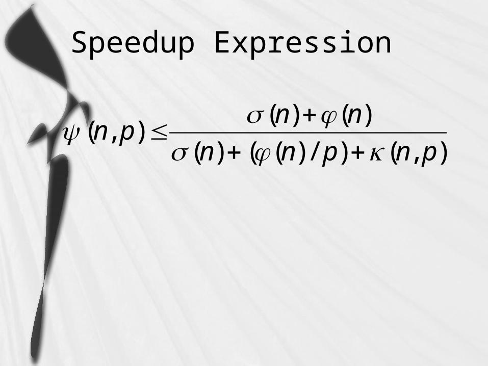
Speedup Expression

),()/)(()(

)()(),(

pnpnn

nnpn

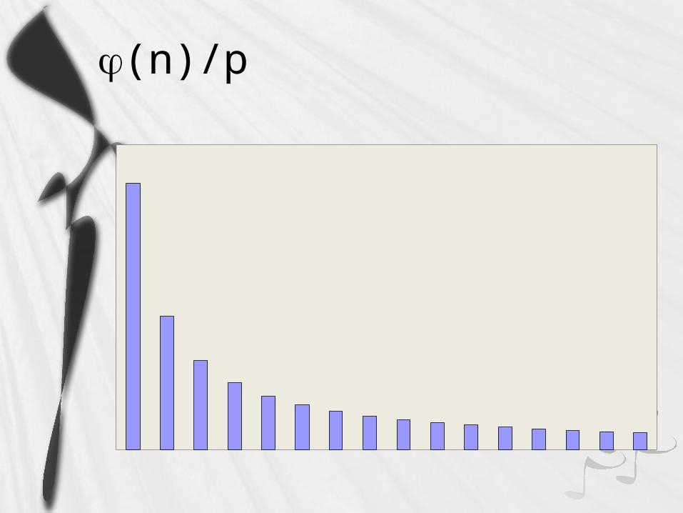
(n)/p

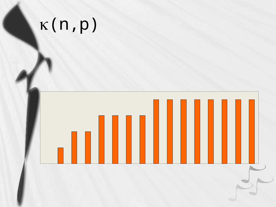
(n,p)

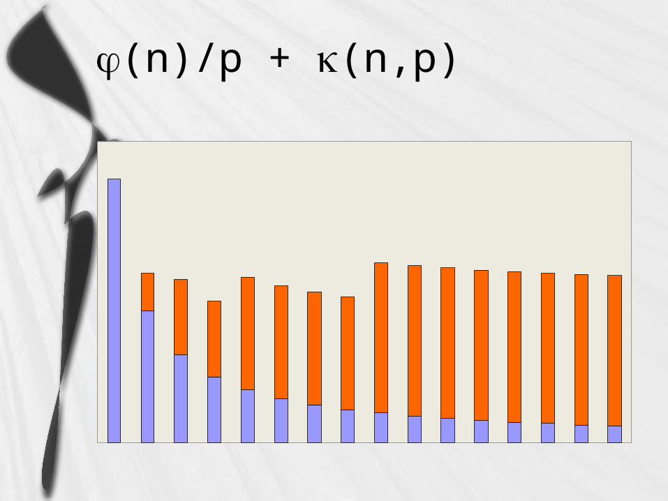
(n)/p + (n,p)

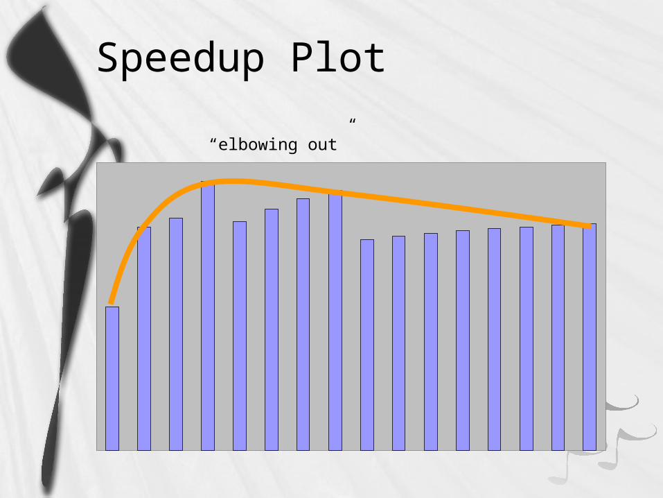
Speedup Plot

“elbowing out”

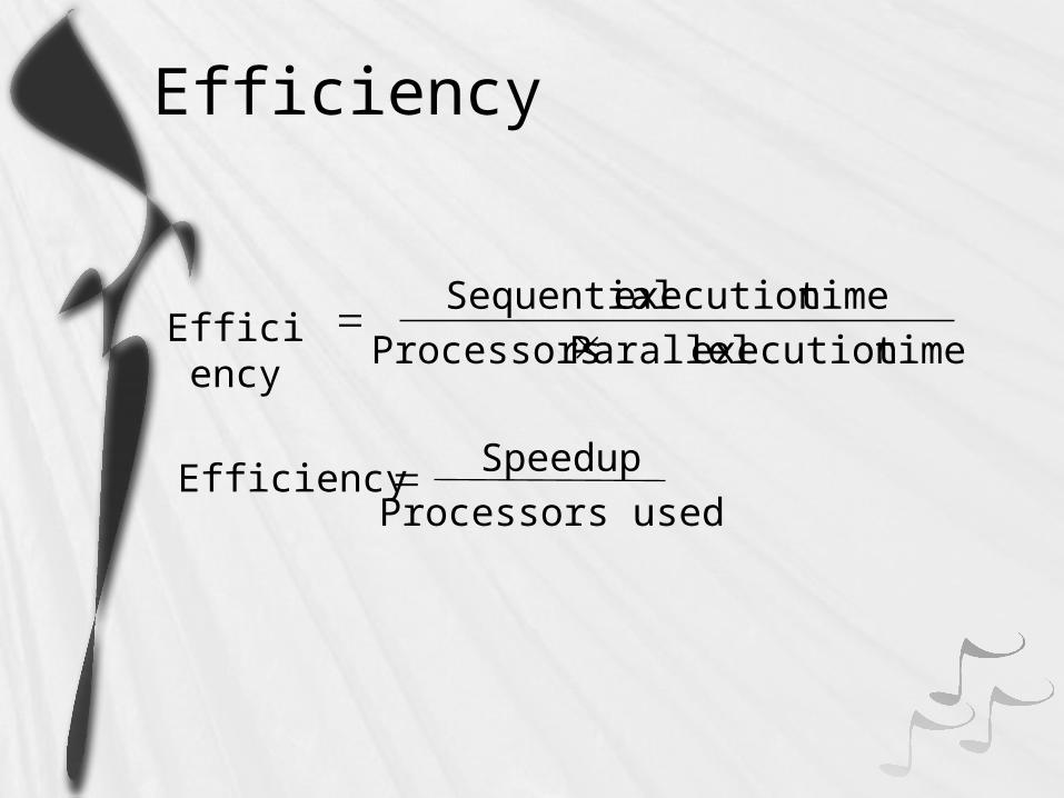
Efficiency

Processors used

Speedup Efficiency

timeexecution Parallel Processors

timeexecution Sequential Efficiency

=

´ =

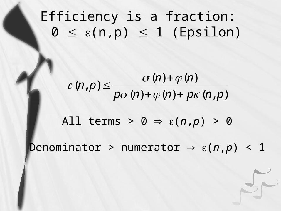
Efficiency is a fraction:0 (n,p) 1 (Epsilon)

),()()(

)()(),(

pnpnnp

nnpn

All terms > 0 (n,p) > 0

Denominator > numerator (n,p) < 1

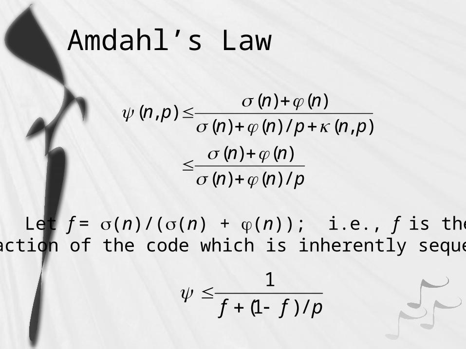
Amdahl’s Law

pnn

nn

pnpnn

nnpn

/)()(

)()(

),(/)()(

)()(),(

Let f = (n)/((n) + (n)); i.e., f is the fraction of the code which is inherently sequential

pff /)1(

1

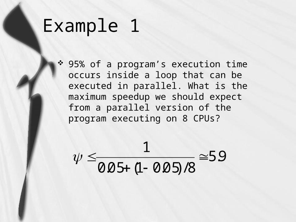
Example 1

95% of a program’s execution time occurs inside a loop that can be executed in parallel. What is the maximum speedup we should expect from a parallel version of the program executing on 8 CPUs?

9.58/)05.01(05.0

1

15CS 491 – Parallel and Distributed Computing

gprof

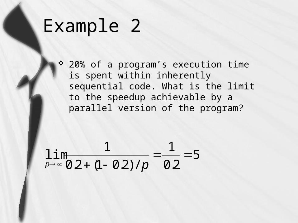
Example 2

20% of a program’s execution time is spent within inherently sequential code. What is the limit to the speedup achievable by a parallel version of the program?

52.0

1

/)2.01(2.0

1lim

pp

Pop Quiz

An oceanographer gives you a serial program and asks you how much faster it might run on 8 processors. You can only find one function amenable to a parallel solution. Benchmarking on a single processor reveals 80% of the execution time is spent inside this function. What is the best speedup a parallel version is likely to achieve on 8 processors?

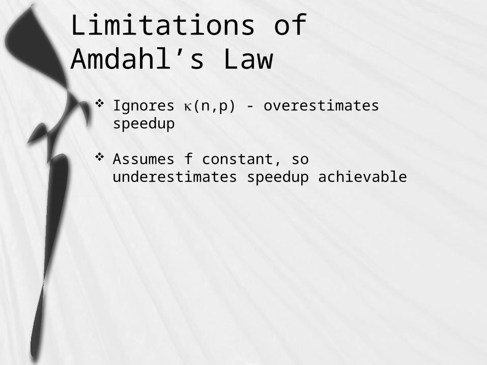
Limitations of Amdahl’s Law

Ignores (n,p) - overestimates speedup

Assumes f constant, so underestimates speedup achievable

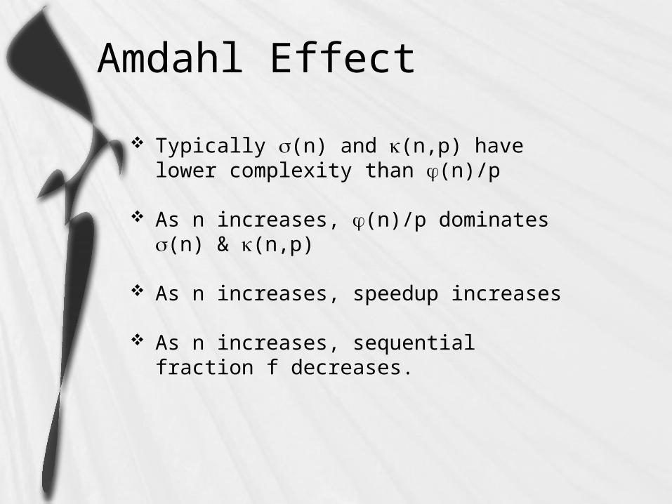
Amdahl Effect

Typically (n) and (n,p) have lower complexity than (n)/p

As n increases, (n)/p dominates (n) & (n,p)

As n increases, speedup increases

As n increases, sequential fraction f decreases.

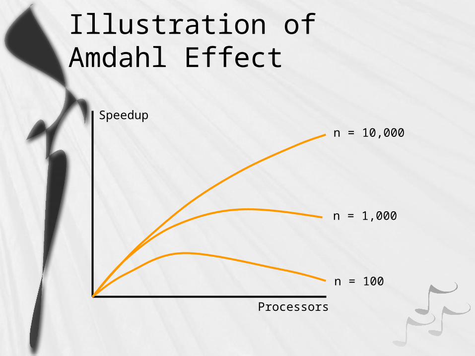
Illustration of Amdahl Effect

n = 100

n = 1,000

n = 10,000

Speedup

Processors

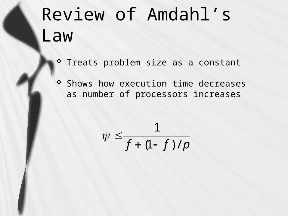
Review of Amdahl’s Law

Treats problem size as a constant

Shows how execution time decreases as number of processors increases

pff /)1(

1

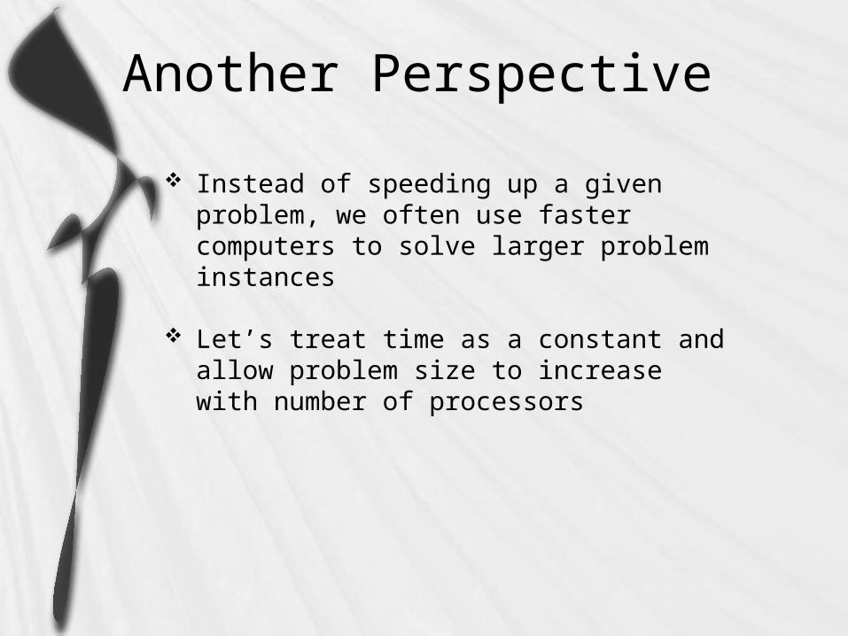
Another Perspective

Instead of speeding up a given problem, we often use faster computers to solve larger problem instances

Let’s treat time as a constant and allow problem size to increase with number of processors

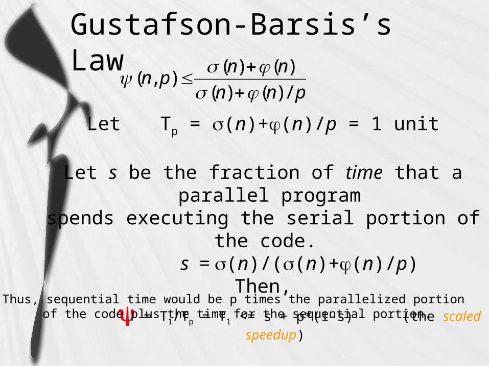
Gustafson-Barsis’s Law

pnn

nnpn

/)()(

)()(),(

Let Tp = (n)+(n)/p = 1 unit

Let s be the fraction of time that a parallel program spends executing the serial portion of the code.

s = (n)/((n)+(n)/p)Then,

= T1/Tp = T1 <= s + p*(1-s) (the scaled speedup)

Thus, sequential time would be p times the parallelized portion of the code plus the time for the sequential portion.

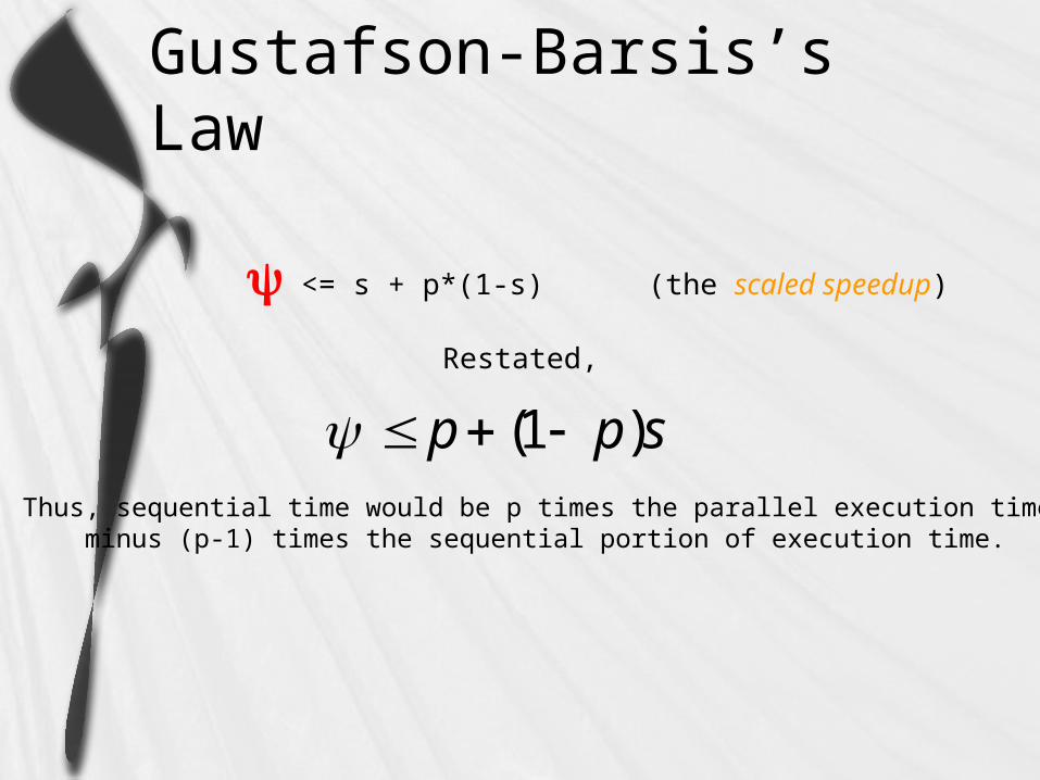
Gustafson-Barsis’s Law

<= s + p*(1-s) (the scaled speedup)

Restated,

spp )1( Thus, sequential time would be p times the parallel execution time

minus (p-1) times the sequential portion of execution time.

Gustafson-Barsis’s Law

Begin with parallel execution time and estimate the time spent in sequential portion.

Predicts scaled speedup (Sp - - same as T1) Why “scaled speedup”?

Estimate sequential execution time to solve same problem (s)

Assumes that s remains fixed irrespective of how large is p - thus overestimates speedup.

Problem size (s + p*(1-s)) is an increasing function of p

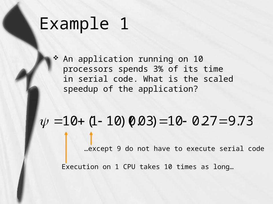
Example 1

An application running on 10 processors spends 3% of its time in serial code. What is the scaled speedup of the application?

73.927.010)03.0)(101(10

Execution on 1 CPU takes 10 times as long…

…except 9 do not have to execute serial code

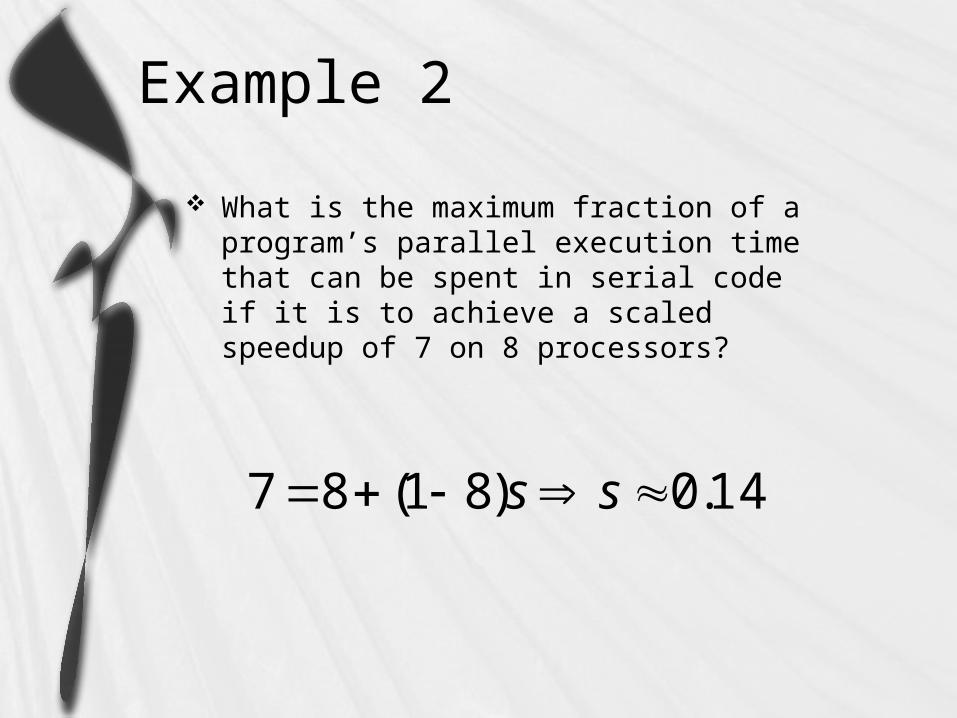
Example 2

What is the maximum fraction of a program’s parallel execution time that can be spent in serial code if it is to achieve a scaled speedup of 7 on 8 processors?

14.0)81(87 ss

Pop Quiz

A parallel program executing on 32 processors spends 5% of its time in sequential code. What is the scaled speedup of this program?

The Karp-Flatt Metric

Amdahl’s Law and Gustafson-Barsis’ Law ignore (n,p)

They can overestimate speedup or scaled speedup

Karp and Flatt proposed another metric

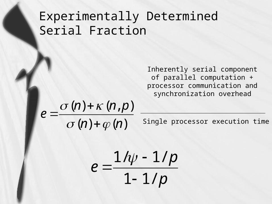
Experimentally Determined Serial Fraction

)()(

),()(

nn

pnne

Inherently serial componentof parallel computation +

processor communication andsynchronization overhead

Single processor execution time

p

pe

/11

/1/1

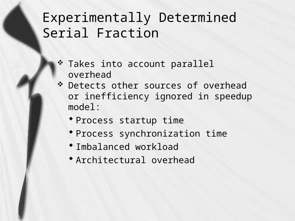
Experimentally Determined Serial Fraction

Takes into account parallel overhead Detects other sources of overhead or

inefficiency ignored in speedup model: Process startup time Process synchronization time Imbalanced workload Architectural overhead

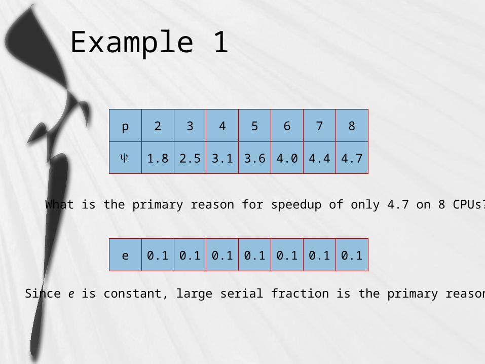
Example 1

p 2 3 4 5 6 7

1.8 2.5 3.1 3.6 4.0 4.4

8

4.7

What is the primary reason for speedup of only 4.7 on 8 CPUs?

e 0.1 0.1 0.1 0.1 0.1 0.1 0.1

Since e is constant, large serial fraction is the primary reason.

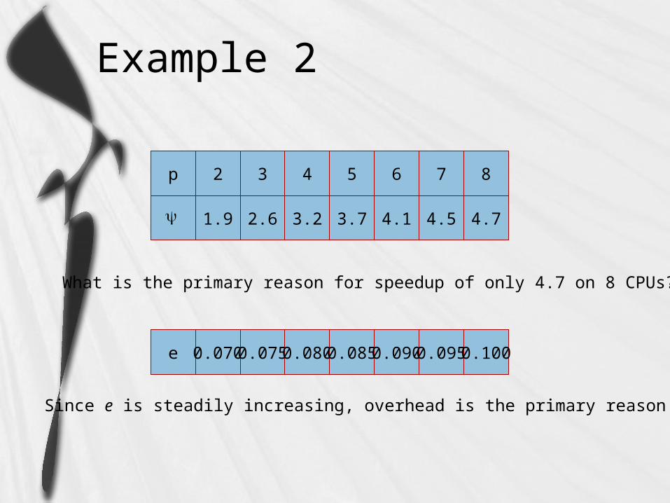
Example 2

p 2 3 4 5 6 7

1.9 2.6 3.2 3.7 4.1 4.5

8

4.7

What is the primary reason for speedup of only 4.7 on 8 CPUs?

e 0.070 0.075 0.080 0.085 0.090 0.095 0.100

Since e is steadily increasing, overhead is the primary reason.

Isoefficiency Metric

Parallel system: parallel program executing on a parallel computer

Scalability of a parallel system: measure of its ability to increase performance as number of processors increases

A scalable system maintains efficiency as processors are added

Isoefficiency: way to measure scalability

This process is also a way to get at what “problem size” mean in the Gustafson-Barsis environment

Isoefficiency Derivation Steps

Begin with speedup formula Compute total amount of overhead Assume efficiency remains constant Determine relation between sequential

execution time and overhead

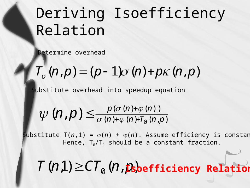
Deriving Isoefficiency Relation

),()()1(),( pnpnppnTo

Determine overhead

Substitute overhead into speedup equation

),()()())()((

0),( pnTnn

nnppn

Substitute T(n,1) = (n) + (n). Assume efficiency is constant. Hence, T0/T1 should be a constant fraction.

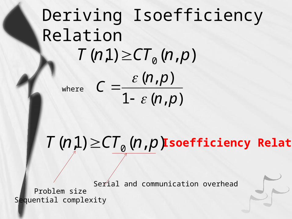
),()1,( 0 pnCTnT Isoefficiency Relation

Deriving Isoefficiency Relation

),(1

),(

pn

pnC

where

Isoefficiency Relation

),()1,( 0 pnCTnT

Problem sizeSequential complexity

Serial and communication overhead

),()1,( 0 pnCTnT

Scalability Function

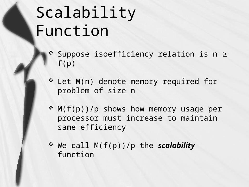
Suppose isoefficiency relation is n f(p)

Let M(n) denote memory required for problem of size n

M(f(p))/p shows how memory usage per processor must increase to maintain same efficiency

We call M(f(p))/p the scalability function

Meaning of Scalability Function

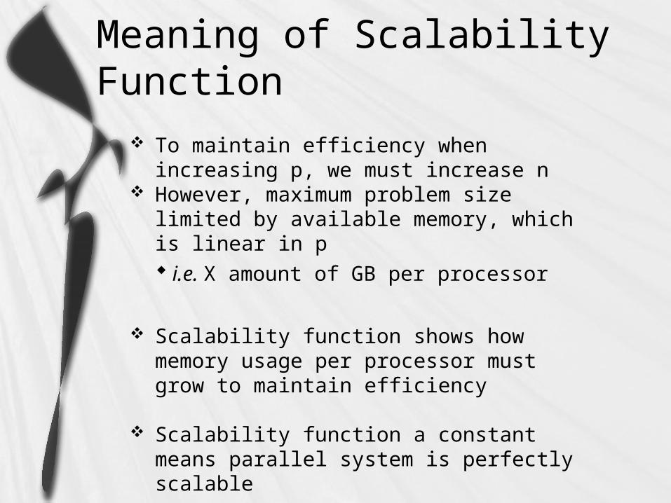
To maintain efficiency when increasing p, we must increase n

However, maximum problem size limited by available memory, which is linear in p i.e. X amount of GB per processor

Scalability function shows how memory usage per processor must grow to maintain efficiency

Scalability function a constant means parallel system is perfectly scalable

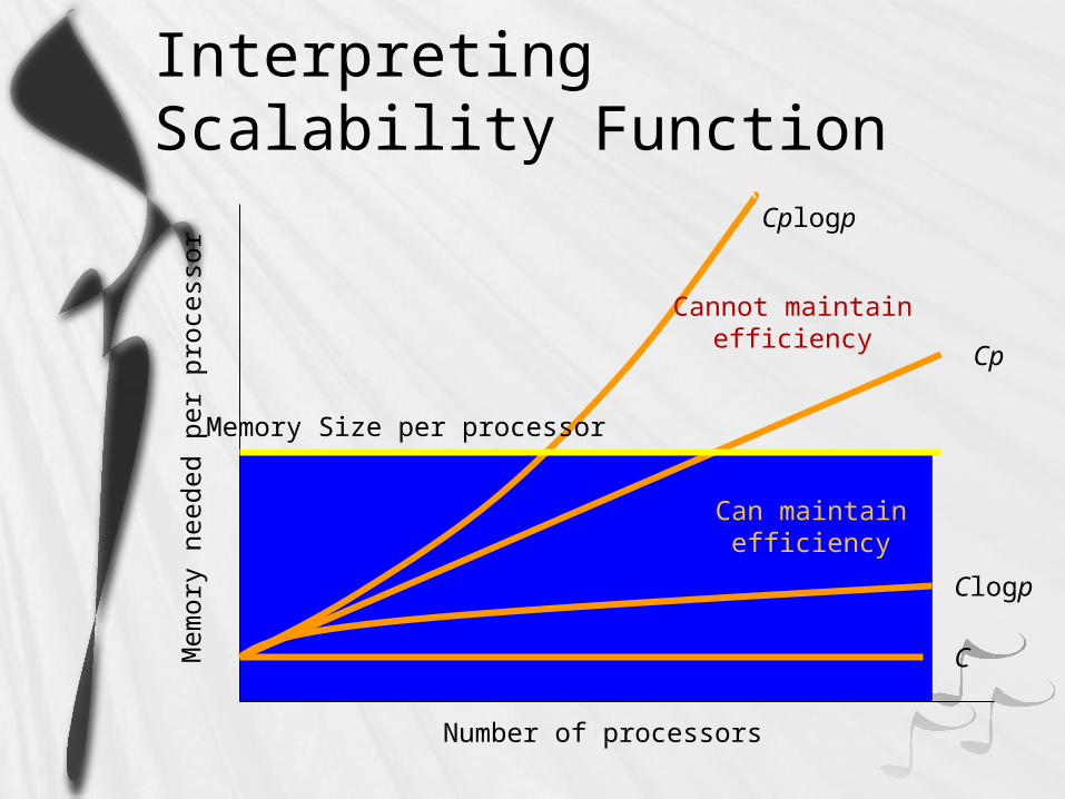
Interpreting Scalability Function

Number of processors

Mem

ory

need

ed p

er p

roce

ssor

Cplogp

Cp

Clogp

C

Memory Size per processor

Can maintainefficiency

Cannot maintainefficiency

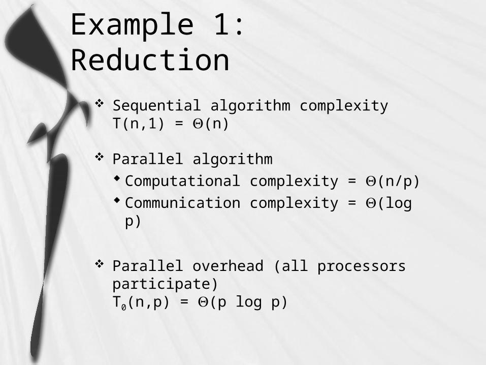
Example 1: Reduction

Sequential algorithm complexityT(n,1) = (n)

Parallel algorithm Computational complexity = (n/p) Communication complexity = (log p)

Parallel overhead (all processors participate)T0(n,p) = (p log p)

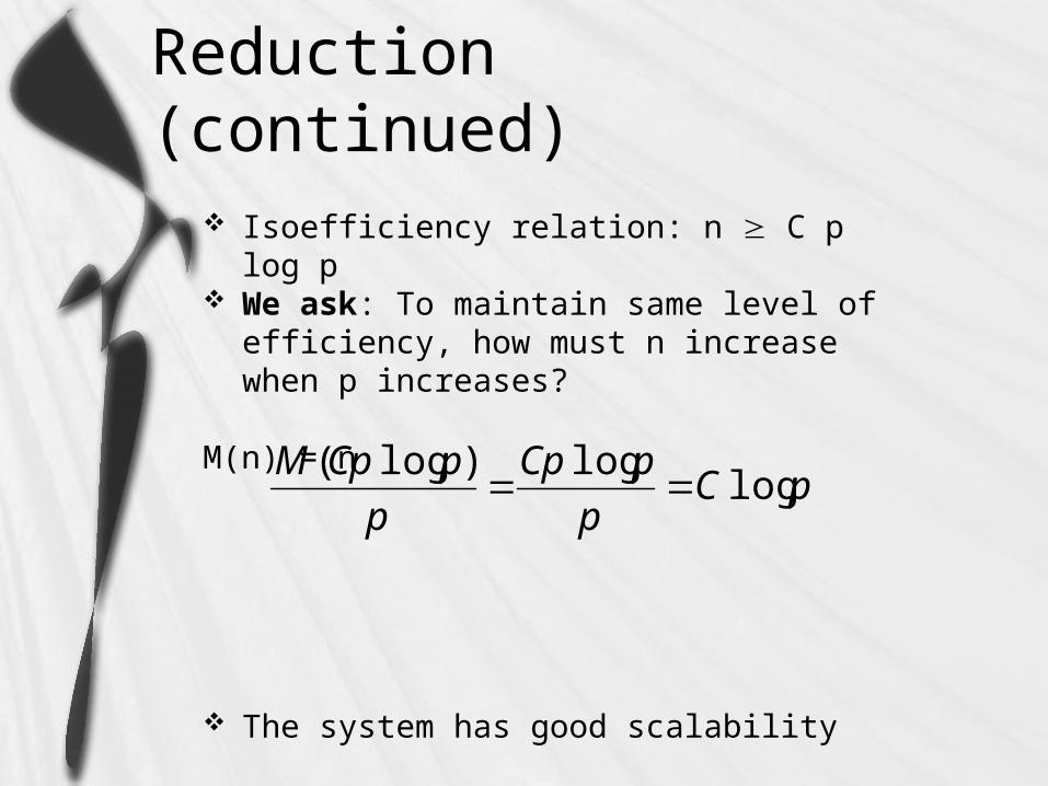
Reduction (continued)

Isoefficiency relation: n C p log p We ask: To maintain same level of

efficiency, how must n increase when p increases?

M(n) = n

The system has good scalability

pCp

pCp

p

pCpMlog

log)log(

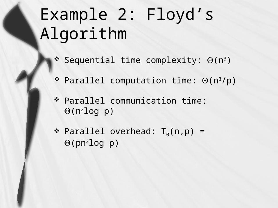
Example 2: Floyd’s Algorithm

Sequential time complexity: (n3)

Parallel computation time: (n3/p)

Parallel communication time: (n2log p)

Parallel overhead: T0(n,p) = (pn2log p)

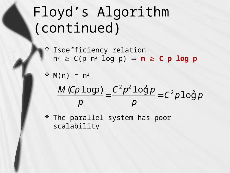
Floyd’s Algorithm (continued)

Isoefficiency relationn3 C(p n2 log p) n C p log p

M(n) = n2

The parallel system has poor scalability

ppCp

ppC

p

pCpM 22222

loglog)log(

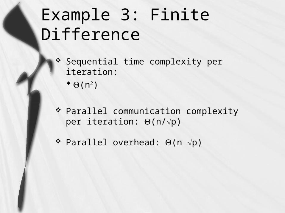
Example 3: Finite Difference

Sequential time complexity per iteration: (n2)

Parallel communication complexity per iteration: (n/p)

Parallel overhead: (n p)

Finite Difference (continued)

Isoefficiency relationn2 Cnp n Cp

M(n) = n2

This algorithm is perfectly scalable

22)(

Cp

pC

p

pCM

Summary (1/3)

Performance terms Speedup Efficiency

Model of speedup Serial component Parallel component Communication component

Summary (2/3)

What prevents linear speedup? Serial operations Communication operations Process start-up Imbalanced workloads Architectural limitations

Summary (3/3)

Analyzing parallel performance Amdahl’s Law Gustafson-Barsis’ Law Karp-Flatt metric Isoefficiency metric