elasto-plastic strain hardening mohr-coulomb...
TRANSCRIPT

double precision, intent(inout) :: ep
double precision, intent(out) :: f
double precision :: c, H
integer, intent(out) :: region, error
if (this%s_type==1) then
error=1
return
else if (this%s_type==2 .or. this%s_type==3) then
allocate(A(4,4))
else if (this%s_type==4) then
allocate(A(6,6))
end if
call this%getcH(ep, c, H)
call toprincipal(sigb, sigbp, A, s_typein=this%s_type)
region=0
f=this%k*sigbp(1,1)-sigbp(3,1)-2*c*sqrt(this%k)
if (f > 0) then
call this%getregion(sigbp, ep, region)
end if
select case(region)
case(0)
sigcp=sigbp
case(1)
call this%returntoMCP(sigbp, ep, sigcp, error)
call this%DepcMCP(sigbp, sigcp, ep, Depcp)
case(2)
call this%returntoMCL1(sigbp, ep, sigcp, error)
call this%DepcMCL1(sigbp, sigcp, ep, Depcp)
case(3)
call this%returntoMCL6(sigbp, ep, sigcp, error)
call this%DepcMCL6(sigbp, sigcp, ep, Depcp)
case(4)
call this%returntoMCS(sigbp, ep, sigcp, error)
call this%DepcMCS(sigbp, sigcp, ep, Depcp)
end select
call fromprincipal(sigcp, sigc, A, Depcp, Depc, s_typein=this%s_type)
end subroutine update
subroutine getregion(this, sigb, ep, region)
implicit none
class(MohrCoulomb) :: this
double precision, dimension(3,1), intent(in) :: sigb
double precision, intent(in) :: ep
double precision, dimension(4,1) :: BPeval
double precision :: c, H, apex
integer, intent(out) :: region
call this%getcH(ep, c, H)
apex=2*c*sqrt(this%k)/(this%k-1)
BPeval(1,1)=dot_product(this%nL1(:,1),sigb(:,1)-apex)
BPeval(2,1)=dot_product(this%nL6(:,1),sigb(:,1)-apex)
BPeval(3,1)=dot_product(this%nP1(:,1),sigb(:,1)-apex)
dododouble precisionon, intent(inout) :: ep
dodoubububle precisionon, intent(out) :: f
doubublelele precision :: c, H
integegerr, intent(out) :: regioion, error
else if (this%s_t_typype==4) then
allocate(A(6,6
end d if
call this%ge
call topri
reregigion
f=
s_type)
subroutine get
implicit none
class(MohrCoulomb) :: this
doub
do
call this%getcH(ep, c, H)
apex=2*c*sqrt(this%k)/(this%k-1)
BPeval(1,1)=dot_product(this%nL1(:,1),sigb(:,1)-apex)
BPeval(2,1)=dot_product(this%nL6(:,1),sigb(:,1)-apex)
BPeval(3,1)= (this%nP1(:,1),sigb(:,1)-apex)
ifif (thisisis%s_typype=e==1) then
errororor=1
reretuturn
elelse iff (thisis%s_t_typype==2=2 . .or. thththis%s_t_typype==3) thenen
alallolocate(A(A(4(4,4))))allocate(A(4,4)) allocate(A(4,4))allocate(A(4,4))
outine get
one
:: this
s_ty
e==4) then_typype=
(6,6
s%ge
opri
gigion
f=
igigcp, , ererror)r)r)
ep, Depcpcp)p)
bp, epepep, sisigcgcgcp,p,p,p, e error)
bp, sisigcp,p, ep, D Depepcp))
toMCMCL6L6(sigbpbp, ep, sigcp,p,p, erroror
pcMCMCL6(s(sigigbp, sisigcgcp, e ep,p, Depepepcp)
his%returnrnrntotoMCMCS(S(sisisigbgbp,p, e ep, sigigcp, erererro
thihis%DepcMCMCMCMCS(sigbp,p, sigcpcpcp, , epep, , DeDepcp)p)
ct
ll frompririncncipipipipipalalalalalalal(sigcp, sigc, A,A, D Depepcp, Depc, s_s_s_ty
end subroutine update
tine g getetreregigion(thihis, sigb, e ep,p, r regegion)n)
one
this
igcpcp
ep,
bpbpbp
bp,
toMC
pcMCMC
his%
thi
ct
llll f
end
outine g
one
this
or)
or
ro
s_s_ty
igcpcp
ep,
bpbpbp
bp,
toMC
pcMCMC
his%
t thihi
ct
llll f
end
or)))
oror))
ror)r)r)
s_tytytypepepeininin=t=t=t=t=this%s%s%s%s_ty
or)
or
ro
s_s_tyty s_ty
e=e==4=4=4) ) ) th
s_t_typypypeieiein=n=ththisisis%s%s_typypype)e)e)e)e)
(t(thihis%s%k)k)k)
=4) the=e=e=
s s_t
(t(t(thi
_typype=e=
(6,6))
s%getcH(H(epep, c,c, H)
opririncncipipipal(sigigb,b, sigbp, A,A, s_t_t
gigionon=0
f=thisis%k%k*s*sigigigbpbpbpbpbpbpbpbp(1(1(1,1,1)-)-sisigbgbp(p(3,3,3,1)1)1)1)-2*c*sqrt(thi
if ( (f f > 0)0) ththenen
call t thihis%getregioion(n(sisigbp, ep,p,p, regioion)n)
e=e==4
s_t
(t(t(thi
_typyp
(6,6
s%
op
gigi
f=
end ifif
selelectct casase(regegioion)n)
cacasese(0)
sigcgcp=p=sigbgbp
case(1(1))
call this%rereturnrntotototoMCP(sisigbgbp, e e ep,p, sigigcp
call t thihis%DeDepcMCMCP(P(P(sigbp, sigcpcpcp, , , ep,
casese(2)
cacallll this%s%returntotoMCMCMCL1(sigigbp,
callll this%DeDepcMCL1(s(s(s(sigigbp,
case(3)
call this%retututurntoMC
call this%DepcpcMCMC
casese(4)
call thihis%
cacall thi
end select
call f
end
igigcp
ep,
igbpbp
bp
toMC
pcMCMC
his%
t thihi
ct
llll f
end
doublele prerecicision, didimensnsion(3(3,1), inin sigb
doublele prerecicision, inintentnt(in) :: ep
doublele prerecicision, didimensnsion(4(4,1) :::: BPevaval
doublele prerecicision :: c, H, , apexex
integeger, ininintent(o(out) :::: r regioion
,1), inin sigb,1), inintent(i(in) :: : ,1), inin sigbsigbdouble precision dimension(3,1 gb
do
,1), gb,1), intent(in),1 sigbgbgb
Emil Smed Sørensen, Aalborg University
M.Sc. 4th Semester, 8 June 2012
Elasto-Plastic Strain Hardening Mohr-Coulomb ModelDerivation and Implementation into the Finite Element Model using Principal Stress Space


School of Engineering
and Science
Sohngårdsholmsvej 57
Telefon 96 35 97 31
Fax 98 13 63 93
http://ses.aau.dk
Title: Elasto-plastic Hardening Mohr-Coulomb Model - Derivation and Implemen-tation into the Finite Element Method UsingPrincipal Stress SpaceTheme: Master ThesisProject period: M.Sc. 4th semester, spring2012Project group: B124CParticipants:
Emil Smed Sørensen
Supervisor: Johan Clausen
Circulation: 3Number of pages:70Submitted: 8th of June 2012
Summary:
The purpose of this report is to derive and implementa strain hardening Mohr-Coulomb model based on re-turn mapping in principal stress space by the use ofboundary planes. The report aims at modeling strainhardening rock material through a Mohr-Coulomb ap-proximation of the generalized Hoek-Brown criterion.Firstly, the classification of rock materials as wellas the generalized Hoek-Brown criterion are pre-sented. Afterwards follows an introduction to theMohr-Coulomb criterion and the approximations usedfor the generalized Hoek-Brown criterion.Next, the fundamentals of plasticity and hardening ispresented along with the theory behind return map-ping in general stress space, including the derivationof the consistent constitutive matrix used in the globalFEM equilibrium iterations. Then the advantages ofreturn mapping in principal stress space is outlined.Following is the derivation of a non-associatedisotropic strain hardening Mohr-Coulomb modelbased on the introduced theory.
Finally, the derived model is implemented in two ex-
amples. The first example tries to model a strip foot-
ing while the second example models a tunnel exca-
vation. The obtained results are compared with per-
fectly plastic solutions utilizing the peak and residual
strength of the rock material.

Contents
1 Introduction 11.1 Statement of Intent. . . . . . . . . . . . . . . . . . . . . . . . . . . . . . . . . . . . . . . 31.2 Prerequisites. . . . . . . . . . . . . . . . . . . . . . . . . . . . . . . . . . . . . . . . . . . 3
2 Classification of Rock Materials and the Generalized Hoek-Brown Criterion 5
3 The Mohr-Coulomb Criterion 93.1 Mohr-Coulomb Approximation of Hoek-Brown criterion. . . . . . . . . . . . . . . . . 10
4 Plasticity Fudamentals 134.1 The Yield Function. . . . . . . . . . . . . . . . . . . . . . . . . . . . . . . . . . . . . . . 134.2 Plastic Potential. . . . . . . . . . . . . . . . . . . . . . . . . . . . . . . . . . . . . . . . . 154.3 Hardening and Softening. . . . . . . . . . . . . . . . . . . . . . . . . . . . . . . . . . . . 154.4 State Parameters. . . . . . . . . . . . . . . . . . . . . . . . . . . . . . . . . . . . . . . . 164.5 Time-Independency. . . . . . . . . . . . . . . . . . . . . . . . . . . . . . . . . . . . . . . 174.6 Infinitesimal Constitutive Matrix. . . . . . . . . . . . . . . . . . . . . . . . . . . . . . . 174.7 Multiple Yield Functions. . . . . . . . . . . . . . . . . . . . . . . . . . . . . . . . . . . . 18
5 Return Mapping in General Stress Space 215.1 Non-linear Finite Element Method. . . . . . . . . . . . . . . . . . . . . . . . . . . . . . 215.2 Return Mapping Basics. . . . . . . . . . . . . . . . . . . . . . . . . . . . . . . . . . . . 225.3 Return to One Active Yield Function. . . . . . . . . . . . . . . . . . . . . . . . . . . . . 245.4 Return to Two Active Yield Functions. . . . . . . . . . . . . . . . . . . . . . . . . . . . 255.5 Return to Three Active Yield Functions. . . . . . . . . . . . . . . . . . . . . . . . . . . 285.6 Determination of Correct Return Type. . . . . . . . . . . . . . . . . . . . . . . . . . . . 28
6 Return Mapping in Principal Stress Space 296.1 Modificaton Matrix. . . . . . . . . . . . . . . . . . . . . . . . . . . . . . . . . . . . . . . 306.2 Boundary Planes. . . . . . . . . . . . . . . . . . . . . . . . . . . . . . . . . . . . . . . . 31
7 Implementation of Strain Hardening Mohr-Coulomb Model 337.1 Basic Premises. . . . . . . . . . . . . . . . . . . . . . . . . . . . . . . . . . . . . . . . . 33
v
vi Contents
7.2 Derivatives. . . . . . . . . . . . . . . . . . . . . . . . . . . . . . . . . . . . . . . . . . . . 337.3 Yield Criterion Regions. . . . . . . . . . . . . . . . . . . . . . . . . . . . . . . . . . . . 347.4 Return Regions and Boundaries. . . . . . . . . . . . . . . . . . . . . . . . . . . . . . . . 367.5 Return Algorithms. . . . . . . . . . . . . . . . . . . . . . . . . . . . . . . . . . . . . . . 387.6 Consistent Constitutive Matrix. . . . . . . . . . . . . . . . . . . . . . . . . . . . . . . . 41
8 Computational Example: Strip Footing 438.1 The Model. . . . . . . . . . . . . . . . . . . . . . . . . . . . . . . . . . . . . . . . . . . . 438.2 Material Parameters. . . . . . . . . . . . . . . . . . . . . . . . . . . . . . . . . . . . . . 448.3 Mesh Coarseness. . . . . . . . . . . . . . . . . . . . . . . . . . . . . . . . . . . . . . . . 458.4 Results. . . . . . . . . . . . . . . . . . . . . . . . . . . . . . . . . . . . . . . . . . . . . . 45
9 Computational Example: Tunnel Excavation 519.1 The model. . . . . . . . . . . . . . . . . . . . . . . . . . . . . . . . . . . . . . . . . . . . 519.2 Material Parameters. . . . . . . . . . . . . . . . . . . . . . . . . . . . . . . . . . . . . . 529.3 Mesh Coarseness. . . . . . . . . . . . . . . . . . . . . . . . . . . . . . . . . . . . . . . . 539.4 Results. . . . . . . . . . . . . . . . . . . . . . . . . . . . . . . . . . . . . . . . . . . . . . 53
10 Conclusion 59
Bibliography 61
Chapter1
Introduction
A large part of the earth’s crust consists of material which can be classified as rock. With advanceswithin the field of civil engineering and the ever growing need for real estate and infrastructure, moreand more structures are build in or on rock material. For some civil engineering structures, this is amajor advantage, since rock material is often very strong and stiff. Properties which are beneficial fora foundation. However, rock material also tends to be quite brittle and posses inferior tensile strength.Properties, which are dangerous to tunnel excavations.
Civil engineering problems involving rock material, as well as many other problems, are often hand-led by the use of finite element modeling, where the generally non-linear governing equations of themodel are discretized into a finite number of elements, for which the solution to thegoverning equationscan be approximated with polynomials. Afterwards the system of equations is solved in an incrementaliterative manner until equilibrium is reached. A crucial part in the finite element method is the choiceof constitutive model, which gives the relationship between the strains and thestresses in a given point.
Part of the constitutive model is to predict when plastic straining of the materialoccurs, which isdictated by the yield criterion. For rock materials, two often used yield criteria are the old-fashionedand thoroughly tested Mohr-Coulomb criterion and the fairly new generalized Hoek-Brown criterion.The Mohr-Coulomb criterion describes a linear relationship between the shear stress in the materialand the corresponding normal stress, which when satisfied, results in plastic straining of the material.The Hoek-Brown criterion is an empirical non-linear refinement of the Mohr-Coulomb criterion andis specifically designed for rock-like materials. However, due to the simplicity of the Mohr-Coulombcriterion, many calculations regarding rock-like material is still carried out using this simpler criterion.
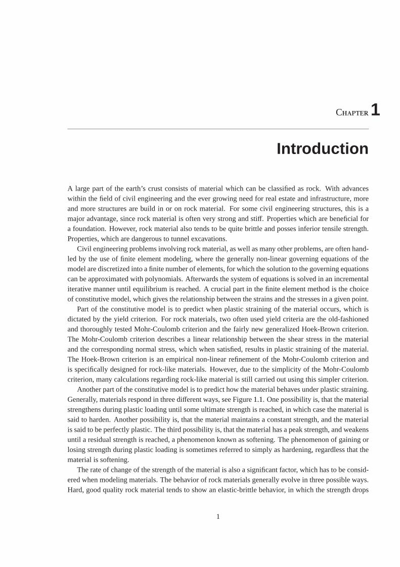
Another part of the constitutive model is to predict how the material behavesunder plastic straining.Generally, materials respond in three different ways, see Figure1.1. One possibility is, that the materialstrengthens during plastic loading until some ultimate strength is reached, in which case the material issaid to harden. Another possibility is, that the material maintains a constant strength, and the materialis said to be perfectly plastic. The third possibility is, that the material has a peakstrength, and weakensuntil a residual strength is reached, a phenomenon known as softening.The phenomenon of gaining orlosing strength during plastic loading is sometimes referred to simply as hardening, regardless that thematerial is softening.
The rate of change of the strength of the material is also a significant factor, which has to be consid-ered when modeling materials. The behavior of rock materials generally evolve in three possible ways.Hard, good quality rock material tends to show an elastic-brittle behavior, in which the strength drops
1
2 Chapter 1. Introduction
Residual strength
Yield strength
Ultimate strength
Initial yield strengthPeak strength
Str
ess
Str
ess
Str
ess
StrainStrainStrain
a) Hardening b) Perfectly plastic c) Softening
Figure 1.1:Material behaviour under plastic loading.
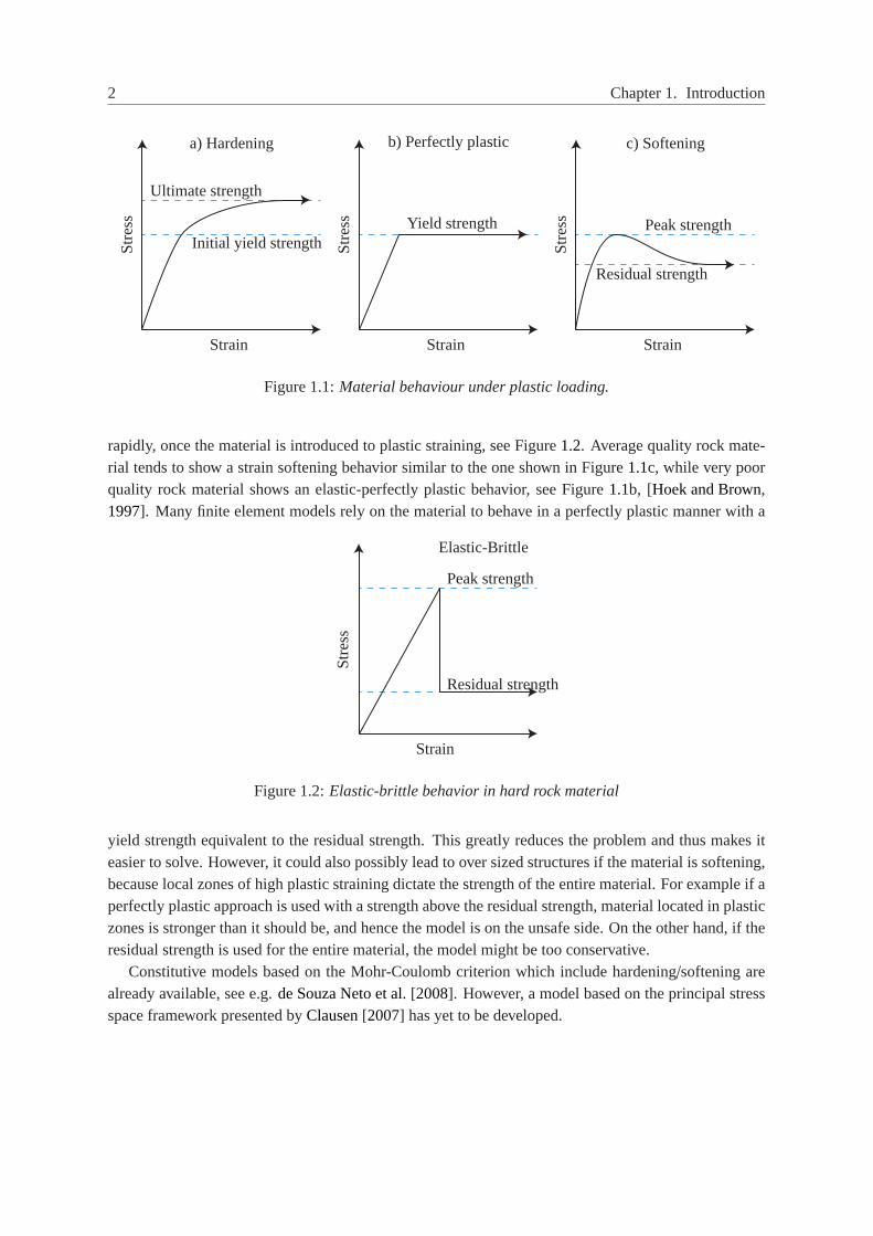
rapidly, once the material is introduced to plastic straining, see Figure1.2. Average quality rock mate-rial tends to show a strain softening behavior similar to the one shown in Figure1.1c, while very poorquality rock material shows an elastic-perfectly plastic behavior, see Figure 1.1b, [Hoek and Brown,1997]. Many finite element models rely on the material to behave in a perfectly plastic manner with a
Elastic-Brittle
Str
ess
Peak strength
Residual strength
Strain
Figure 1.2:Elastic-brittle behavior in hard rock material
yield strength equivalent to the residual strength. This greatly reduces the problem and thus makes iteasier to solve. However, it could also possibly lead to over sized structures if the material is softening,because local zones of high plastic straining dictate the strength of the entirematerial. For example if aperfectly plastic approach is used with a strength above the residual strength, material located in plasticzones is stronger than it should be, and hence the model is on the unsafe side. On the other hand, if theresidual strength is used for the entire material, the model might be too conservative.
Constitutive models based on the Mohr-Coulomb criterion which include hardening/softening arealready available, see e.g.de Souza Neto et al.[2008]. However, a model based on the principal stressspace framework presented byClausen[2007] has yet to be developed.
1.1. Statement of Intent 3
1.1 Statement of Intent
The aim of this project is to derive a strain hardening/softening constitutive model for use in finiteelement calculations based on the Mohr-Coulomb criterion which utilize derivations in principal stressspace, both regarding the updated stress state and the consistent constitutive matrix needed for theglobal equilibrium iterations.
To test and demonstrate the usefulness of the model, it is used to estimate the influence of thehardening/softening properties on the bearing capacity of a strip footing as well as therisk of failureduring a tunnel excavation.
1.2 Prerequisites
Strains and stresses are tensors of the 2nd order and the constitutive relation between them is a 4thorder tensor. However, symmetric properties of the strain and stress tensors allow for a formulation inwhich they can be expressed equally accurate as vectors, and the constitutive relation can be expressedas a matrix. In this report, the latter formulation will be used due to its simplicity and ease of use whenwriting computer code. Throughout the report, a number of variables, vectors and matrices are used.To keep track of these, a number of guidelines will be presented in the following.
A scalar is presented in ordinary text asσ1, whereas a vector or a matrix is symbolized in bold ase.g.σσσ or DDD. By default, vectors are 6×1 and matrices are 6×6. Vectors and matrices with an overline,e.g. σσσ andDDD are related to the principal stress components and have dimensions of 3×1 and 3×3respectively. Vectors and matrices with a tilde, e.g.σσσ andTTT are related to the shear stress componentsand have dimensions of 3×1 and 3×3 respectively. Vectors and matrices with a hat, e.g.σσσ andDDD arefull 6×1 vectors and 6×6 matrices, where the axes are aligned with those of the principal stresses.
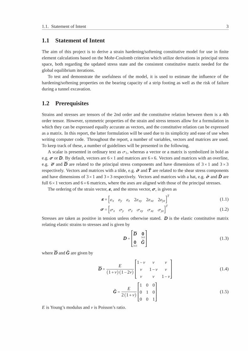
The ordering of the strain vector,εεε, and the stress vector,σσσ, is given as
εεε = [εx εy εz 2εxy 2εxz 2εyz]T (1.1)
σσσ = [σx σy σz σxy σxz σyz]T (1.2)
Stresses are taken as positive in tension unless otherwise stated.DDD is the elastic constitutive matrixrelating elastic strains to stresses and is given by
DDD =⎡⎢⎢⎢⎢⎢⎣DDD 000
3x3
0003x3
GGG
⎤⎥⎥⎥⎥⎥⎦(1.3)
whereDDD andGGG are given by
DDD = E(1+ν)(1−2ν)⎡⎢⎢⎢⎢⎢⎢⎣1−ν ν ν
ν 1−ν ν
ν ν 1−ν⎤⎥⎥⎥⎥⎥⎥⎦
(1.4)
GGG = E
2(1+ν)⎡⎢⎢⎢⎢⎢⎢⎣1 0 0
0 1 0
0 0 1
⎤⎥⎥⎥⎥⎥⎥⎦(1.5)
E is Young’s modulus andν is Poisson’s ratio.

Chapter2
Classification of Rock Materials and theGeneralized Hoek-Brown Criterion
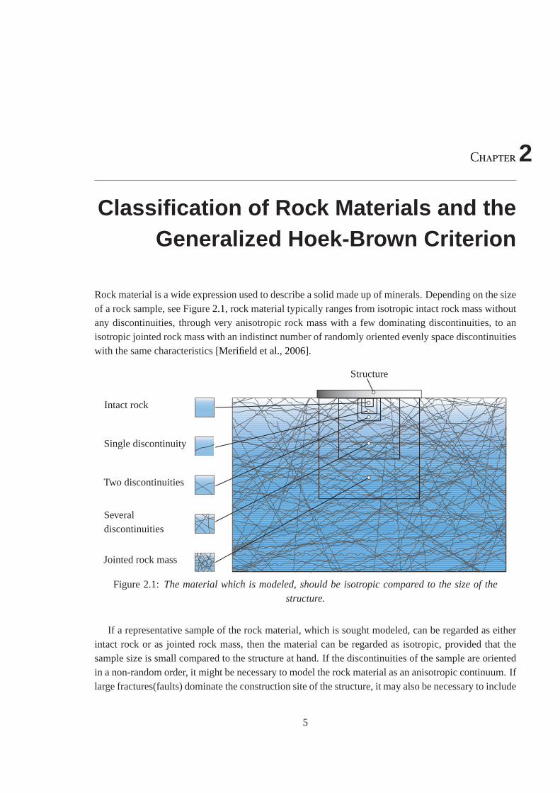
Rock material is a wide expression used to describe a solid made up of minerals. Depending on the sizeof a rock sample, see Figure2.1, rock material typically ranges from isotropic intact rock mass withoutany discontinuities, through very anisotropic rock mass with a few dominating discontinuities, to anisotropic jointed rock mass with an indistinct number of randomly oriented evenlyspace discontinuitieswith the same characteristics [Merifield et al., 2006].
Intact rock
Single discontinuity
Two discontinuities
Severaldiscontinuities
Jointed rock mass
Structure
Figure 2.1:The material which is modeled, should be isotropic compared to the size of thestructure.
If a representative sample of the rock material, which is sought modeled, canbe regarded as eitherintact rock or as jointed rock mass, then the material can be regarded as isotropic, provided that thesample size is small compared to the structure at hand. If the discontinuities of the sample are orientedin a non-random order, it might be necessary to model the rock material asan anisotropic continuum. Iflarge fractures(faults) dominate the construction site of the structure, it mayalso be necessary to include
5
6 Chapter 2. Classification of Rock Materials and the Generalized Hoek-Brown Criterion
such fractures in the model mesh. In the following, it is assumed, that the rock material can be modeledas an isotropic continuum.
In order to be able to include rock material in finite element models, the properties of the rockmaterial need to be known and somehow quantified. Extensive empirical research has lead to theformulation of the generalized Hoek-Brown criterion, equation (2.1), which predict the stress statesthat cause failure in rock materials [Hoek and Brown, 1997].
σ′1 =σ′3+σci(mbσ′3
σci+ s)a
(2.1)
σ′1 andσ′3 are the major and minor effective principal stresses respectively, where compression is takenas positive. As the criterion suggests, four parameters are needed in order to asses the strength ofthe rock material, namely the uniaxial compressive strength of the intact rockmaterial,σci, and theconstantsmb, s anda. The constants can be estimated based on the Geological Strength Index(GSI),the disturbance factor,D, and the intact rock material constant,mi , by using the following expressions[Hoek et al., 2002]
mb =mi exp(GSI−10028−14D
) (2.2)
s= exp(GSI−1009−3D
) (2.3)
a= 12+ 1
6(exp(−GSI
15)−exp(−20
3)) (2.4)
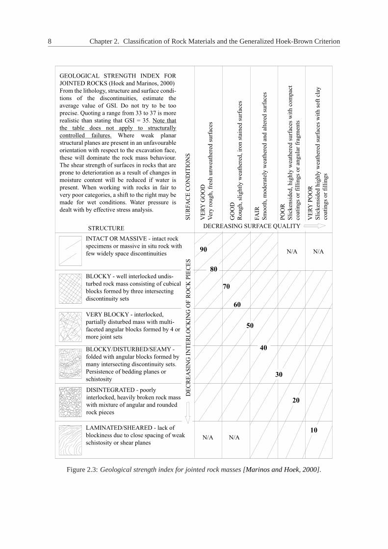
The Geological Strength Index is a measure of the rock material’s quality based on field observations,which takes into account the composition and structure of the in-situ rock material as well as the surfaceconditions, see Figure2.3 on page8. Based on this, the GSI is assigned on a scale ranging from 0 to100, where 100 indicates a very good quality [Hoek, 2007].
The disturbance factor,D, is used to take into account the blast damage, that part of the rock mate-rial might suffer from. It ranges from 0 to 1, where 0 indicates undisturbed rock material. The materialconstantmi and the uniaxial compressive strength of the intact rock material,σci, is found using labo-ratory tests on the intact rock material. The elastic modulus of the rock material can be estimated by[Hoek and Diederichs, 2006]
Erm = 100,000 MPa( 1−D/21+exp((75+25D−GS I)/11)) (2.5)
Once the rock material has reached a stress state which causes failure, itloses some of its strength,as mentioned inchapter 1. The manner in which the strength drops is not entirely determined, butthree possible characteristics are mentioned inHoek and Brown[1997]. One possibility is to assume anelastic-brittle behavior, where the strength of the rock material rapidly drops to some residual strengthonce the failure criteria is reached, see Figure1.2. Another possibility is to assume a strain soften-ing relationship between the strength of the material and the plastic straining which it undergoes, seeFigure1.1c. The third options is to assume that the rock material exhibits in a elastic-perfectly plasticway, see Figure1.1b. In this report, it is assumed that the rock material behaves in a strain-softeningmanner. For an implementation of an elastic-perfectly plastic generalized Hoek-Brown criterion seeClausen[2007] andSørensen[2012].
Chapter 2. Classification of Rock Materials and the Generalized Hoek-Brown Criterion 7
In order to conform with most finite element codes, where tension is taken aspositive, the gener-alised Hoek-Brown criterion can be expressed as
σ3 =σ1−σci(s−mbσ1
σci)a
(2.6)
where the apostrophes signifying effective stresses have been omitted for simplicity. In order to expressthe above as a yield function, resulting in a negative number for elastic statesand a positive number fornon-allowable states, it can further be rewritten to the following
f (σσσ,σci,s,mb,a) =σ1−σ3−σci(s−mbσ1
σci)a = 0 (2.7)
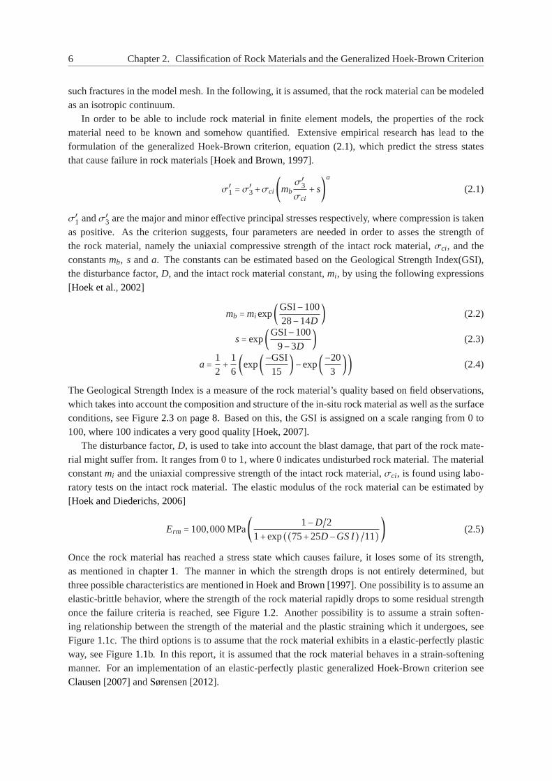
The stress states which are solutions to the above equation form a six sided pyramid along the hydro-static axis with curved sides as can be seen in Figure2.2. Any stress state inside the pyramid is elastic,whereas any stress state located outside is unobtainable.
σ3
σ2
σ1
Hydrostatic axis,σ1 =σ2 =σ3
Figure 2.2:The generalized Hoek-Brown criterion visualized in principal stress space.
8 Chapter 2. Classification of Rock Materials and the Generalized Hoek-Brown Criterion
GEOLOGICAL STRENGTH INDEX FOR
JOINTED ROCKS (Hoek and Marinos, 2000)
From the lithology, structure and surface condi-
tions of the discontinuities, estimate the
average value of GSI. Do not try to be too
precise. Quoting a range from 33 to 37 is more
realistic than stating that GSI = 35. Note that
the table does not apply to structurally
controlled failures. Where weak planar
structural planes are present in an unfavourable
orientation with respect to the excavation face,
these will dominate the rock mass behaviour.
The shear strength of surfaces in rocks that are
prone to deterioration as a result of changes in
moisture content will be reduced if water is
present. When working with rocks in fair to
very poor categories, a shift to the right may be
made for wet conditions. Water pressure is
dealt with by effective stress analysis.
SU
RFA
CE
CO
ND
ITIO
NS
STRUCTURE
INTACT OR MASSIVE - intact rock
specimens or massive in situ rock with
few widely space discontinuities
BLOCKY - well interlocked undis-
turbed rock mass consisting of cubical
blocks formed by three intersecting
discontinuity sets
VERY BLOCKY - interlocked,
partially disturbed mass with multi-
faceted angular blocks formed by 4 or
more joint sets
BLOCKY/DISTURBED/SEAMY -
folded with angular blocks formed by
many intersecting discontinuity sets.
Persistence of bedding planes or
schistosity
DISINTEGRATED - poorly
interlocked, heavily broken rock mass
with mixture of angular and rounded
rock pieces
LAMINATED/SHEARED - lack of
blockiness due to close spacing of weak
schistosity or shear planes
DE
CR
EA
SIN
G I
NT
ER
LO
CK
ING
OF
RO
CK
PIE
CE
S
VE
RY
GO
OD
Ver
y r
ough, fr
esh u
nw
eath
ered
surf
aces
FA
IR
Sm
ooth
, m
oder
atel
y w
eath
ered
and a
lter
ed s
urf
aces
GO
OD
Rough, sl
ightl
y w
eath
ered
, ir
on s
tain
ed s
urf
aces
PO
OR
Sli
cken
sided
, hig
hly
wea
ther
ed s
urf
aces
wit
h c
om
pac
t
coat
ings
or
fill
ings
or
angula
r fr
agm
ents
VE
RY
PO
OR
Sli
cken
sided
hig
hly
wea
ther
ed s
urf
aces
wit
h s
oft
cla
y
coat
ings
or
fill
ings
DECREASING SURFACE QUALITY
N/A N/A
N/A N/A90
80
70
60
50
40
30
20
10
Figure 2.3:Geological strength index for jointed rock masses [Marinos and Hoek, 2000].
Chapter3
The Mohr-Coulomb Criterion
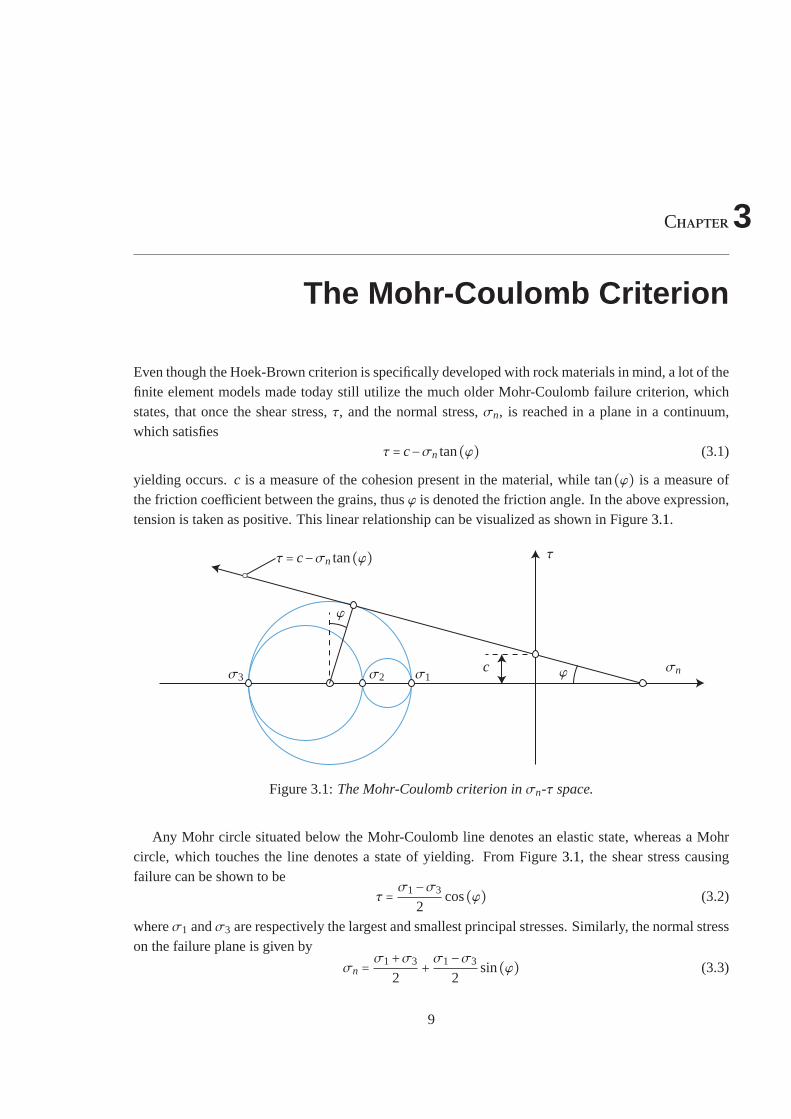
Even though the Hoek-Brown criterion is specifically developed with rock materials in mind, a lot of thefinite element models made today still utilize the much older Mohr-Coulomb failure criterion, whichstates, that once the shear stress,τ, and the normal stress,σn, is reached in a plane in a continuum,which satisfies
τ = c−σn tan(ϕ) (3.1)
yielding occurs.c is a measure of the cohesion present in the material, while tan(ϕ) is a measure ofthe friction coefficient between the grains, thusϕ is denoted the friction angle. In the above expression,tension is taken as positive. This linear relationship can be visualized as shown in Figure3.1.
σ1σ2σ3c ϕ
ϕ
τ = c−σn tan(ϕ) τ
σn
Figure 3.1:The Mohr-Coulomb criterion inσn-τ space.
Any Mohr circle situated below the Mohr-Coulomb line denotes an elastic state, whereas a Mohrcircle, which touches the line denotes a state of yielding. From Figure3.1, the shear stress causingfailure can be shown to be
τ = σ1−σ3
2cos(ϕ) (3.2)
whereσ1 andσ3 are respectively the largest and smallest principal stresses. Similarly, thenormal stresson the failure plane is given by
σn = σ1+σ3
2+ σ1−σ3
2sin(ϕ) (3.3)
9
10 Chapter 3. The Mohr-Coulomb Criterion
Substitution back into (3.1) and rewriting results in
σ1−σ3+(σ1+σ3)sin(ϕ) = 2ccos(ϕ) (3.4)
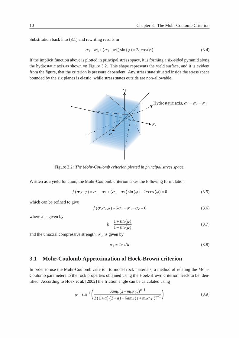
If the implicit function above is plotted in principal stress space, it is forming a six-sided pyramid alongthe hydrostatic axis as shown on Figure3.2. This shape represents the yield surface, and it is evidentfrom the figure, that the criterion is pressure dependent. Any stress state situated inside the stress spacebounded by the six planes is elastic, while stress states outside are non-allowable.
σ1
σ2
σ3
Hydrostatic axis,σ1 =σ2 =σ3
Figure 3.2:The Mohr-Coulomb criterion plotted in principal stress space.
Written as a yield function, the Mohr-Coulomb criterion takes the following formulation
f (σσσ,c,ϕ) =σ1−σ3+(σ1+σ3)sin(ϕ)−2ccos(ϕ) = 0 (3.5)
which can be refined to givef (σσσ,σc,k) = kσ1−σ3−σc = 0 (3.6)
wherek is given by
k= 1+sin(ϕ)1−sin(ϕ) (3.7)
and the uniaxial compressive strength,σc, is given by
σc = 2c√
k (3.8)
3.1 Mohr-Coulomb Approximation of Hoek-Brown criterion
In order to use the Mohr-Coulomb criterion to model rock materials, a method of relating the Mohr-Coulomb parameters to the rock properties obtained using the Hoek-Brown criterion needs to be iden-tified. According toHoek et al.[2002] the friction angle can be calculated using
ϕ = sin−1( 6amb(s+mbσ3n)a−1
2(1+a)(2+a)+6amb(s+mbσ3n)a−1) (3.9)
3.1. Mohr-Coulomb Approximation of Hoek-Brown criterion 11
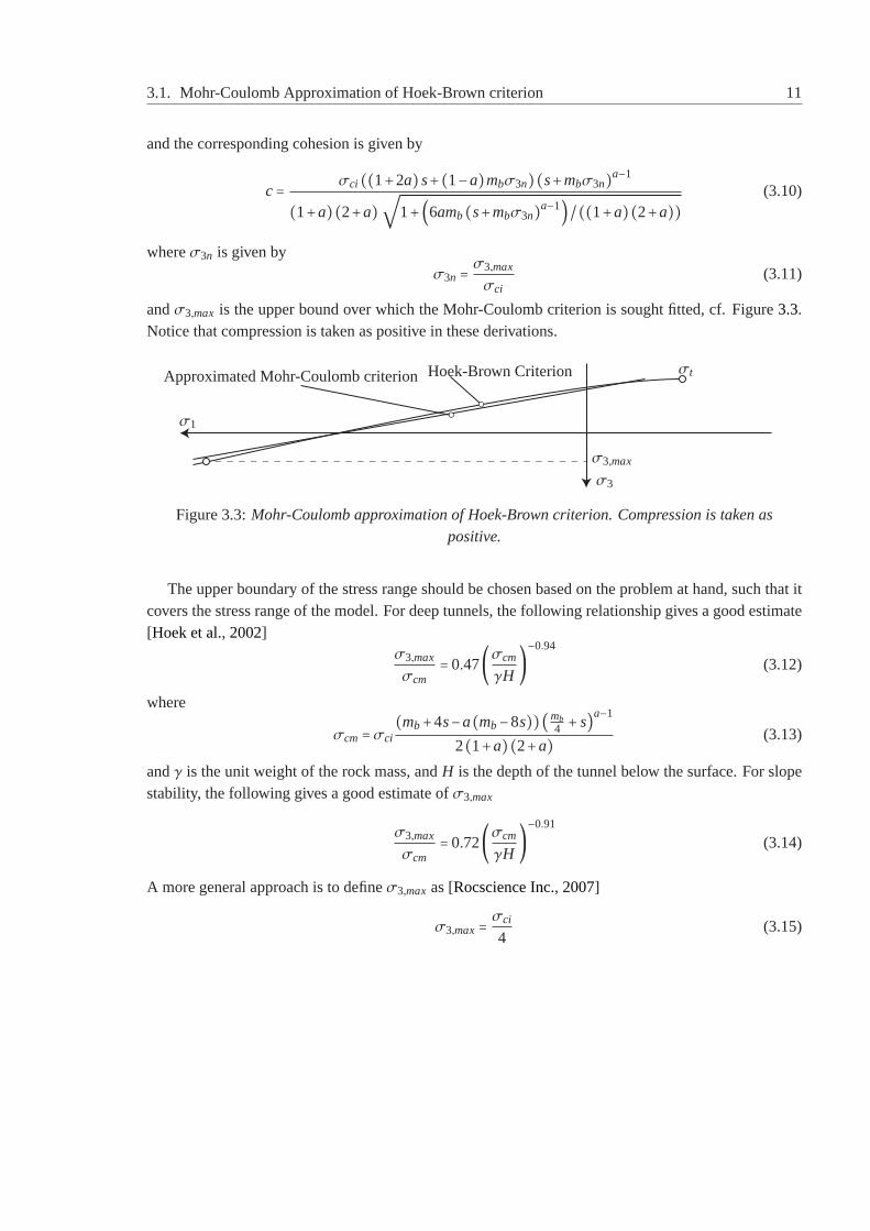
and the corresponding cohesion is given by
c= σci ((1+2a)s+(1−a)mbσ3n)(s+mbσ3n)a−1
(1+a)(2+a) √1+(6amb(s+mbσ3n)a−1)/((1+a)(2+a)) (3.10)
whereσ3n is given byσ3n = σ3,max
σci(3.11)
andσ3,max is the upper bound over which the Mohr-Coulomb criterion is sought fitted, cf. Figure3.3.Notice that compression is taken as positive in these derivations.
σ1
σ3
σ3,max
σtApproximated Mohr-Coulomb criterionHoek-Brown Criterion
Figure 3.3:Mohr-Coulomb approximation of Hoek-Brown criterion. Compression istaken aspositive.
The upper boundary of the stress range should be chosen based on the problem at hand, such that itcovers the stress range of the model. For deep tunnels, the following relationship gives a good estimate[Hoek et al., 2002]
σ3,max
σcm= 0.47(σcm
γH)−0.94
(3.12)
where
σcm=σci(mb+4s−a(mb−8s))(mb
4 + s)a−1
2(1+a)(2+a) (3.13)
andγ is the unit weight of the rock mass, andH is the depth of the tunnel below the surface. For slopestability, the following gives a good estimate ofσ3,max
σ3,max
σcm= 0.72(σcm
γH)−0.91
(3.14)
A more general approach is to defineσ3,max as [Rocscience Inc., 2007]
σ3,max= σci
4(3.15)

Chapter4
Plasticity Fudamentals
In this chapter, some of the basics of material plasticity is outlined. However, adetailed descriptionis beyond the scope of this report. For a more thorough exposition, seede Souza Neto et al.[2008],Ottosen and Ristinmaa[2005] andCrisfield[2000].
4.1 The Yield Function
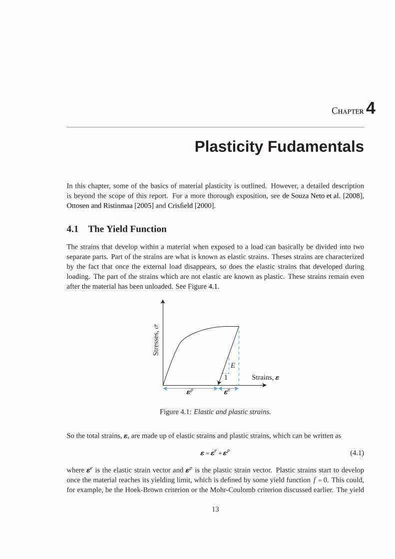
The strains that develop within a material when exposed to a load can basicallybe divided into twoseparate parts. Part of the strains are what is known as elastic strains. Theses strains are characterizedby the fact that once the external load disappears, so does the elastic strains that developed duringloading. The part of the strains which are not elastic are known as plastic.These strains remain evenafter the material has been unloaded. See Figure4.1.
Str
esse
s,σ
Strains,εεε
εεεp εεεe
1
E
Figure 4.1:Elastic and plastic strains.
So the total strains,εεε, are made up of elastic strains and plastic strains, which can be written as
εεε = εεεe+εεεp (4.1)
whereεεεe is the elastic strain vector andεεεp is the plastic strain vector. Plastic strains start to developonce the material reaches its yielding limit, which is defined by some yield functionf = 0. This could,for example, be the Hoek-Brown criterion or the Mohr-Coulomb criterion discussed earlier. The yield
13
14 Chapter 4. Plasticity Fudamentals
function, f , is a function of the stresses as well as some hardening parameters,KKK, which describe thestrength of the material, i.e.
f = f (σσσ,KKK) (4.2)
Sometimes, a material might require more than one yield function in order to be modeled sufficientlyaccurate, this is discussed insection 4.7. The hardening parameters are usually determined by somestate parameters,κκκ, that determine the internal state of the material
KKK =KKK (κκκ) (4.3)
The yield function is a scalar valued function, which gives a negative value for all stress states that areelastic. Once the yield function reaches a value of zero, plastic strains start to develop. The stress stateswhich fulfill this criterion form a surface in stress space known as the yieldsurface, see e.g. Figure2.2and3.2. Further, the yield function remains zero during plastic loading, which implies that the timederivative of f during plastic loading is zero, which can be written as
d f
dt= ∂ f
∂t
dt
dt+( ∂ f
∂σσσ)T dσσσ
dt+( ∂ f
∂KKK)T ∂KKK
∂κκκ
dκκκ
dt= 0 (4.4)
which is known as the consistency relation. Since the yield function is time-independent, it simplifiesto
d f
dt=aaaT dσσσ
dt+( ∂ f
∂KKK)T ∂KKK
∂κκκ
dκκκ
dt= 0 (4.5)
whereaaa is given by
aaa= ∂ f
∂σσσ(4.6)
The time-dependency is discussed further insection 4.5. A stress state which returns a positive valueof the yield function is inadmissible. The stress state within the material is determinedby the elasticstrains through the constitutive matrix,DDD, as
σσσ =DDDεεεe=DDD(εεε−εεεp) (4.7)
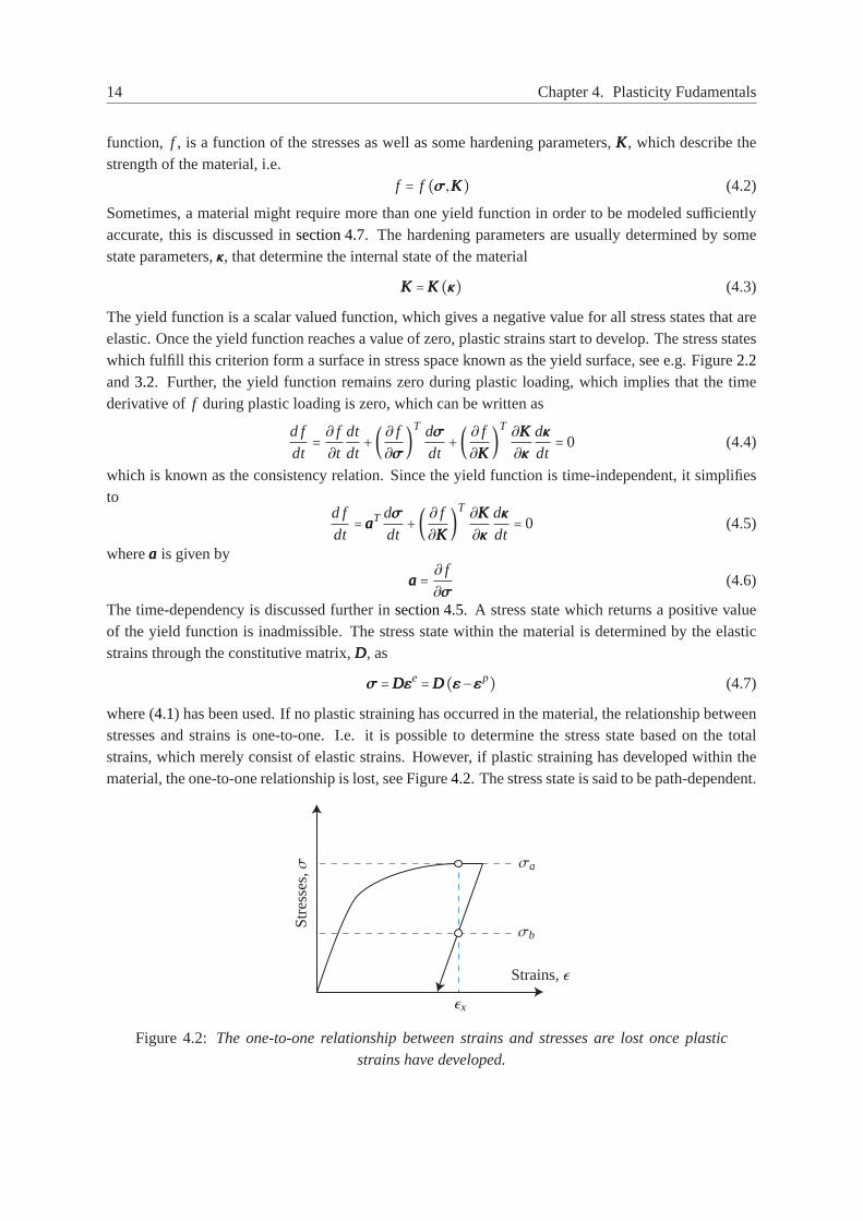
where (4.1) has been used. If no plastic straining has occurred in the material, the relationship betweenstresses and strains is one-to-one. I.e. it is possible to determine the stressstate based on the totalstrains, which merely consist of elastic strains. However, if plastic straininghas developed within thematerial, the one-to-one relationship is lost, see Figure4.2. The stress state is said to be path-dependent.
Str
esse
s,σ
Strains,ǫ
σa
σb
ǫx
Figure 4.2: The one-to-one relationship between strains and stresses are lost onceplasticstrains have developed.
4.2. Plastic Potential 15
Because of this path-dependence, it is necessary to adopt an incremental approach in order to findmatching strain-stress relations. This is done by taking the time derivative of (4.7), which can bewritten as
dσσσ
dt=DDD
dεεε
dt=DDD(dεεε
dt− dεεεp
dt) (4.8)
4.2 Plastic Potential
Once the yield function reaches zero and plastic strains start to develop, itis crucial to know in whichdirection they develop. However there is no conclusive way to determine this. A way to get aroundthis, is to define a plastic potential function,g. The plastic potential is a scalar valued function, whichusually depends upon the stress state and some hardening parameters
g= g(σσσ,KKK) (4.9)
The partial derivative of this plastic potential with respect to the stresses define the direction of theplastic strains. A common choice for the plastic potential is to use the yield function. If this is the case,it is referred to as associated plasticity. If another function is chosen, it isreferred to as non-associatedplasticity. The length of the incremental plastic strain is controlled by a so called plastic multiplier,dλ,which is a non-negative scalar. Thus the plastic strain increment is given by
dεεεp
dt= dλ
dt
∂g
∂σσσ= dλ
dtbbb (4.10)
where the abbreviationbbb has been introduced to improve readability. This relation is known as the flowrule.
4.3 Hardening and Softening
As mentioned earlier, rock material tend to lose some of its strength once plastic straining occurs,which is known as softening. However many metals tend to show an increase instrength during plasticstraining, see Figure1.1a, which is known as hardening. Usually both phenomena are simply referredto as hardening. If the material is considered perfectly plastic, the yield criterion is independent of thehardening parametersKKK, and simply reduces to
f (σσσ,KKK) = f (σσσ) = F (σσσ) = 0 (4.11)
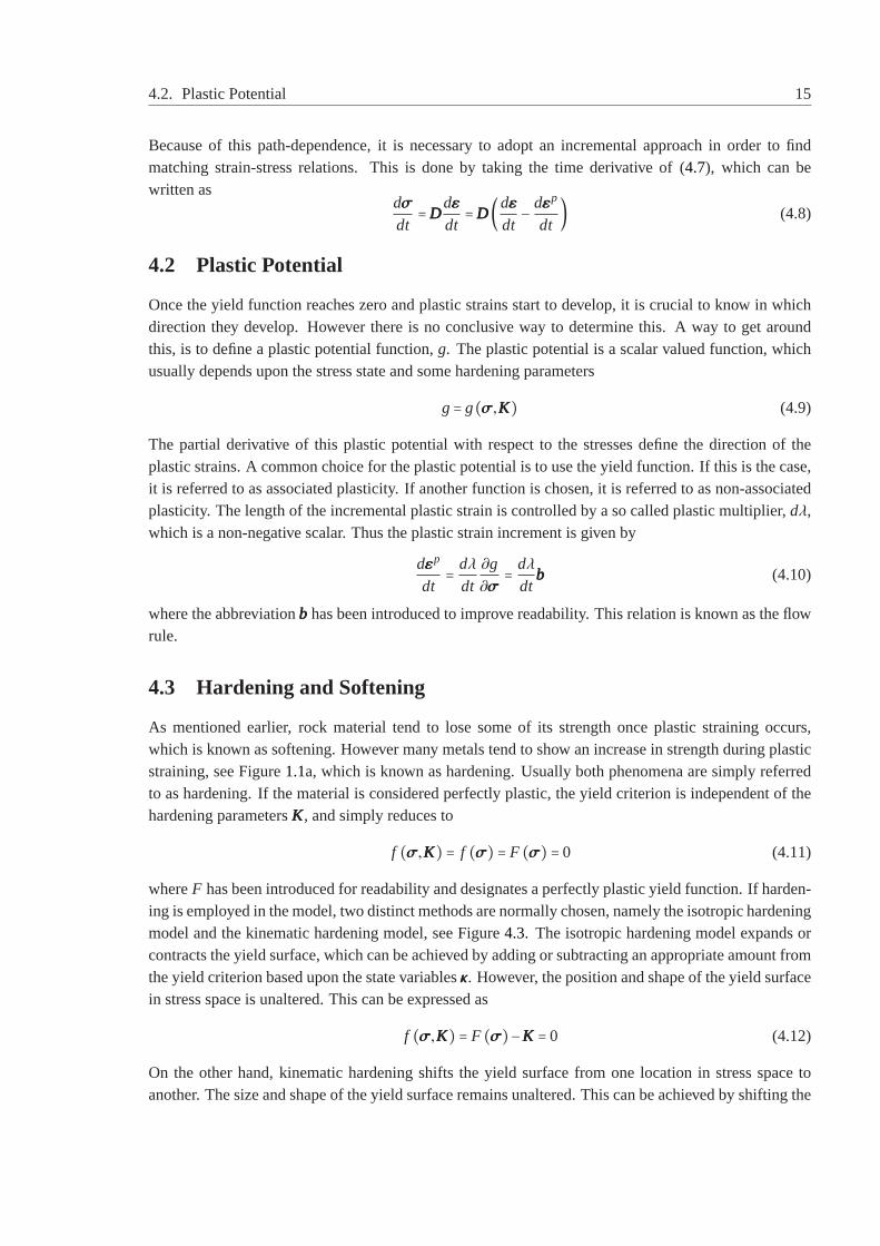
whereF has been introduced for readability and designates a perfectly plastic yieldfunction. If harden-ing is employed in the model, two distinct methods are normally chosen, namely the isotropic hardeningmodel and the kinematic hardening model, see Figure4.3. The isotropic hardening model expands orcontracts the yield surface, which can be achieved by adding or subtracting an appropriate amount fromthe yield criterion based upon the state variablesκκκ. However, the position and shape of the yield surfacein stress space is unaltered. This can be expressed as
f (σσσ,KKK) = F (σσσ)−KKK = 0 (4.12)
On the other hand, kinematic hardening shifts the yield surface from one location in stress space toanother. The size and shape of the yield surface remains unaltered. Thiscan be achieved by shifting the
16 Chapter 4. Plasticity Fudamentals
stresses by some amount defined by the state variables as
f (σσσ,KKK) = F (σσσ−KKK) = 0 (4.13)
The two different hardening models can be used simultaneously, in which case it is referred to as mixedhardening. Mixed hardening alters the size and position of the yield surface and leaves the shapeunaltered. This can be written as
f (σσσ,KKK) = F (σσσ−KKKkin)−KKK iso= 0 (4.14)
whereKKKkin andKKK iso are the hardening parameters associated with kinematic hardening and isotropichardening respectively.
F (σσσ)F (σσσ)F (σσσ)
F (σσσ)−KKK F (σσσ−KKK)F (σσσ−KKKkin)−KKK iso
Figure 4.3:Isotropic, kinematic and mixed hardening.
4.4 State Parameters
The state parameters which control the hardening of the material need to be identified and their time rateof change has to be established, the so-called evolution law. The two most common state parametersare the accumulated plastic strain, denoted,εp, and the dissipated plastic work,Wp, defined by
Wp = ∫ εεεp
0σσσTdεεεp (4.15)
The accumulated plastic strain can be defined in different manners, in which the most common is theVon Mises accumulated plastic strain defined by
εp = ∫ t
0
√23(dεεεp
dt)T dεεεp
dtdt (4.16)
Alternatively, the state parameters can also be defined by some potential function, j, which is a functionof the stress state and the hardening variables
j = j (σσσ,KKK) (4.17)
4.5. Time-Independency 17
and a plastic multiplier, using the following expression
dκκκ
dt= −dλ
dt
∂ j
∂KKK(4.18)
For instance, if the state parameter is the accumulated plastic strain,εp, and the hardening parameter isthe cohesion,c, the increment of the accumulated plastic strain is given as
dεp
dt= −dλ
dt
∂ j
∂c(4.19)
If j is assumed equal tof , the evolution law is said to be associated, and ifj is different from f , theevolution law is said to be non-associated.
4.5 Time-Independency
As can be seen from the above equations, there are a lot of first ordertime derivatives, which representthe load rate of the problem. If a solution is sought, which is independent of the load rate, these timerate of changes can simply be thought of as changes in the variables whichare being differentiated. Forexample, the time rate of change of the plastic strains
dεεεp
dt(4.20)
can be replaced withdεεεp (4.21)
and thought of as a nothing more than an infinitesimal change in the plastic strains, regardless of time.By adopting this independency, the consistency relation, equation (4.5), can be written as
d f =aaaTdσσσ+( ∂ f
∂KKK)T ∂KKK
∂κκκdκκκ = 0 (4.22)
The stress increment, equation (4.8), can be written as
dσσσ =DDD(dεεε−dεεεp) (4.23)
The flow rule, equation (4.10), can be written as
dεεεp = dλbbb (4.24)
and finally, the evolution law defined by a potential function, equation (4.18), can be written as
dκκκ = −dλ∂ j
∂KKK(4.25)
4.6 Infinitesimal Constitutive Matrix
The infinitesimal constitutive matrix,DDDep, relates infinitesimal strain increments with infinitesimalstress increments as follows
dσσσ =DDDepdεεε (4.26)
18 Chapter 4. Plasticity Fudamentals
Combining the consistency relation, equation (4.22), the infinitesimal stress increment, equation (4.23),the plastic flow rule, equation (4.24), and the evolution law, a solution for the infinitesimal incrementof the plastic multiplier,dλ, can be found. If the hardening law is assumed to be defined by a potentialfunction, j, as in equation (4.25), dλ is found to be
dλ = aaaTDDDdεεε
aaaTDDDbbb+( ∂ f∂KKK )T ∂KKK
∂κκκ
∂ j∂KKK
(4.27)
If this solution is substituted back into equation (4.23), the infinitesimal constitutive matrix can be foundto be
DDDep=DDD− DDDbbbaaaTDDD
aaaTDDDbbb+( ∂ f∂KKK )T ∂KKK
∂κκκ
∂ j∂KKK
(4.28)
4.7 Multiple Yield Functions
Some yield criteria might consist of multiple yield functions
f1(σσσ,KKK) , f2(σσσ,KKK) , . . . , fn(σσσ,KKK) (4.29)
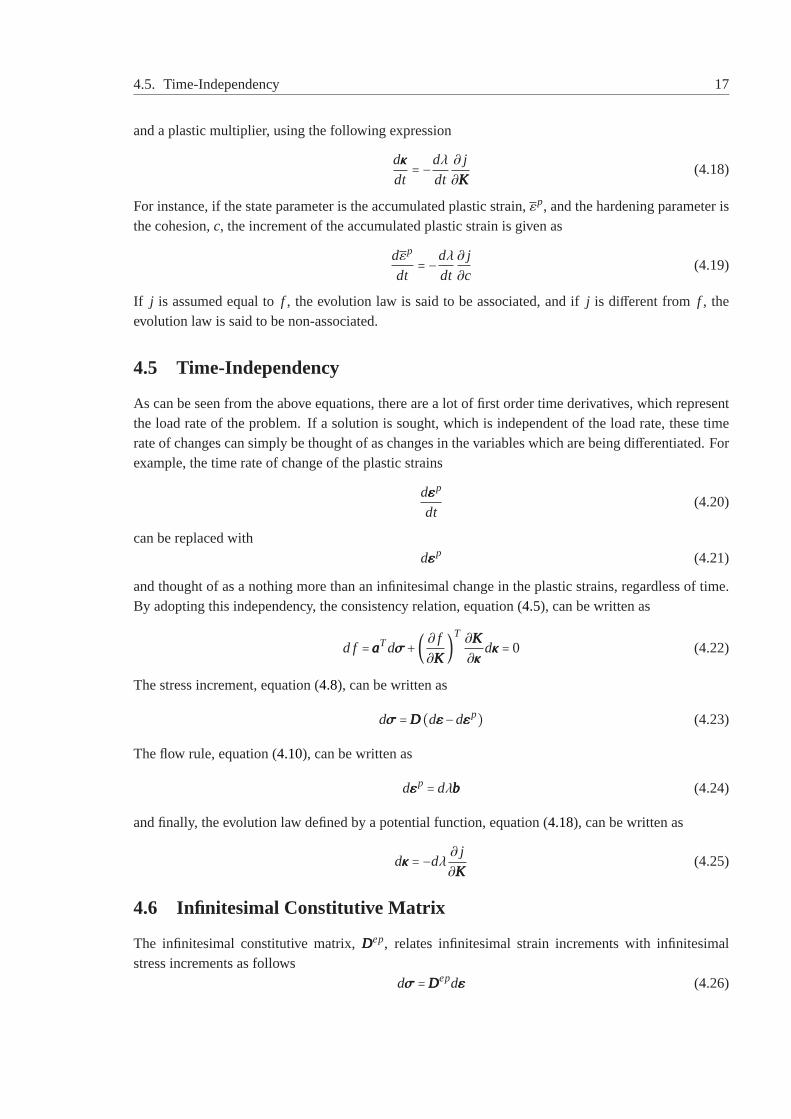
Each yield function defines a surface in stress space. In this case, the elastic stress states are boundedby the stress states which return a negative value of all the yield functions.See Figure4.4
f1 = 0
f2 = 0
f1 < 0
f2 < 0
f1 < 0∩ f2 < 0
Discontinuity
Discontinuity
Figure 4.4:The elastic stress states (blue) of a yield criterion with multiple yield functions(green).
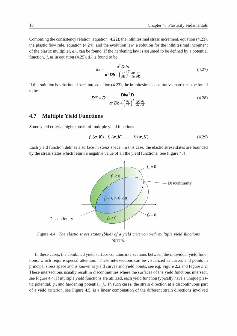
In these cases, the combined yield surface contains intersections betweenthe individual yield func-tions, which require special attention. These intersections can be visualized as curves and points inprincipal stress space and is known as yield curves and yield points, seee.g. Figure2.2and Figure3.2.These intersections usually result in discontinuities where the surfaces ofthe yield functions intersect,see Figure4.4. If multiple yield functions are utilized, each yield function typically have a unique plas-tic potential,gi , and hardening potential,j i . In such cases, the strain direction at a discontinuous partof a yield criterion, see Figure4.5, is a linear combination of the different strain directions involved
4.7. Multiple Yield Functions 19
[Koiter, 1953]
dεεεp = k∑i=1
dλibbbi (4.30)
wherek is the number of plastic potentials, that is part of the intersection at hand. Similarly, theevolution law is given by
dκκκ = − k∑i=1
dλi∂ j i∂KKK
(4.31)
bbb1
bbb2
dεεε
f1 < 0∩ f2 < 0 f1
f2
Figure 4.5:The plastic strain direction at a discontinues part of the yield criteria.

Chapter5
Return Mapping in General StressSpace
In this chapter, the theory behind return mapping is introduced. However,a short introduction to thenon-linear finite element method is given first, in order show the need and applicability of return map-ping. For a more detailed description of the theory behind return mapping andfinite element methods,seede Souza Neto et al.[2008], Cook et al.[2002] andCrisfield[2000]. The derivations of this chapterrely on a evolution law of the form given by equation (4.25) and (4.31).
5.1 Non-linear Finite Element Method
Problems involving the displacement and stress distribution throughout a modelcan be formulatedas partial differential equations made up of the governing equations behind the problem and someboundary conditions, which make the model unique. However, for complexmodels, an analyticalsolution to these boundary value problems is very hard or simply impossible to establish. Becauseof this, the problem is sought solved through numerical integration, which iswhere the finite elementmethod comes into play.
As the name suggests, the model is discretized into a finite number of elements, for which thesolution to the governing equations can be approximated with polynomials. A large range of differentelements exist, each with advantages and disadvantages, however this is beyond the scope of this report.Based on this discretization, the stiffness of the entire model can be calculated. Because the stiffnessof the model is non-linear and path dependent, the boundary conditions are applied incrementally inwhat is known as load steps. The system of equations is solved iteratively ineach load step, to makesure that equilibrium is fulfilled. Usually by the use of a Newton-Raphson scheme. This process can beschematized as shown in Table5.1. The highlighted points of the procedure are material dependent andis the main focus of this report. The updated stress state should ideally be found through and integrationof the infinitesimal elasto-plastic constitutive matrix along the path of the strain increment as
σσσk =σσσk−1+∫ εεεk−1+∆εεε
εεεk−1
dσσσ =σσσk−1+∫ εεεk−1+∆εεε
εεεk−1
DDDepdεεε (5.1)
where equation (4.26) has been used. However, the integration of equation (5.1) is no easy task, sincethe strain path is unknown andDDDep is stress dependent. Several methods exist, which try to circumventthis problem. Return mapping is one of these methods, and is the method used throughout this report.
21
22 Chapter 5. Return Mapping in General Stress Space
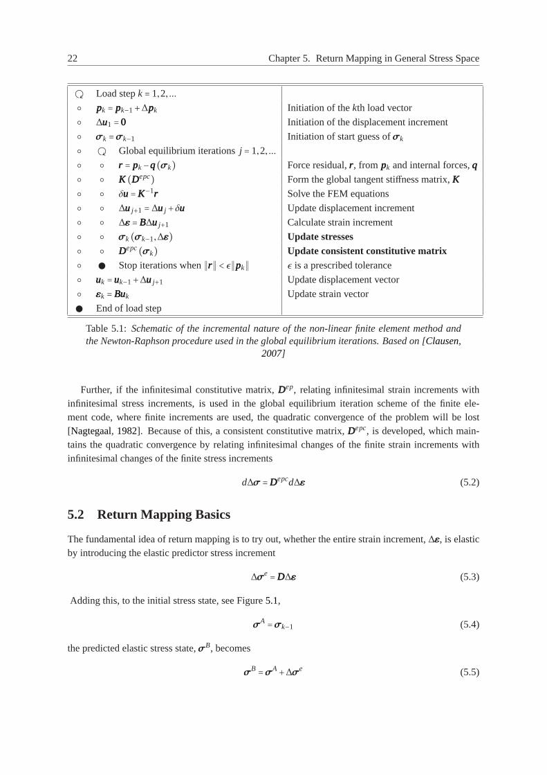
ÿ Load stepk= 1,2, ...○ pppk = pppk−1+∆pppk Initiation of thekth load vector○ ∆uuu1 =000 Initiation of the displacement increment○ σσσk =σσσk−1 Initiation of start guess ofσσσk○ ÿ Global equilibrium iterationsj = 1,2, ...○ ○ rrr = pppk−qqq(σσσk) Force residual,rrr, from pppk and internal forces,qqq○ ○ KKK (DDDepc) Form the global tangent stiffness matrix,KKK○ ○ δuuu=KKK−1rrr Solve the FEM equations○ ○ ∆uuu j+1 = ∆uuu j +δuuu Update displacement increment○ ○ ∆εεε =BBB∆uuu j+1 Calculate strain increment○ ○ σσσk(σσσk−1,∆εεε) Update stresses○ ○ DDDepc(σσσk) Update consistent constitutive matrix○ Stop iterations when∥rrr∥ < ǫ∥pppk∥ ǫ is a prescribed tolerance○ uuuk =uuuk−1+∆uuu j+1 Update displacement vector○ εεεk =BBBuuuk Update strain vector
End of load step
Table 5.1:Schematic of the incremental nature of the non-linear finite element methodandthe Newton-Raphson procedure used in the global equilibrium iterations. Based on [Clausen,
2007]
Further, if the infinitesimal constitutive matrix,DDDep, relating infinitesimal strain increments withinfinitesimal stress increments, is used in the global equilibrium iteration scheme of the finite ele-ment code, where finite increments are used, the quadratic convergenceof the problem will be lost[Nagtegaal, 1982]. Because of this, a consistent constitutive matrix,DDDepc, is developed, which main-tains the quadratic convergence by relating infinitesimal changes of the finitestrain increments withinfinitesimal changes of the finite stress increments
d∆σσσ =DDDepcd∆εεε (5.2)
5.2 Return Mapping Basics
The fundamental idea of return mapping is to try out, whether the entire strain increment,∆εεε, is elasticby introducing the elastic predictor stress increment
∆σσσe=DDD∆εεε (5.3)
Adding this, to the initial stress state, see Figure5.1,
σσσA =σσσk−1 (5.4)
the predicted elastic stress state,σσσB, becomes
σσσB =σσσA+∆σσσe (5.5)
5.2. Return Mapping Basics 23
∆σσσe -∆σσσp
∆σσσ
σσσA
σσσB
σσσC
f (σσσA,KKKA) = 0
f (σσσC,KKKC) = 0
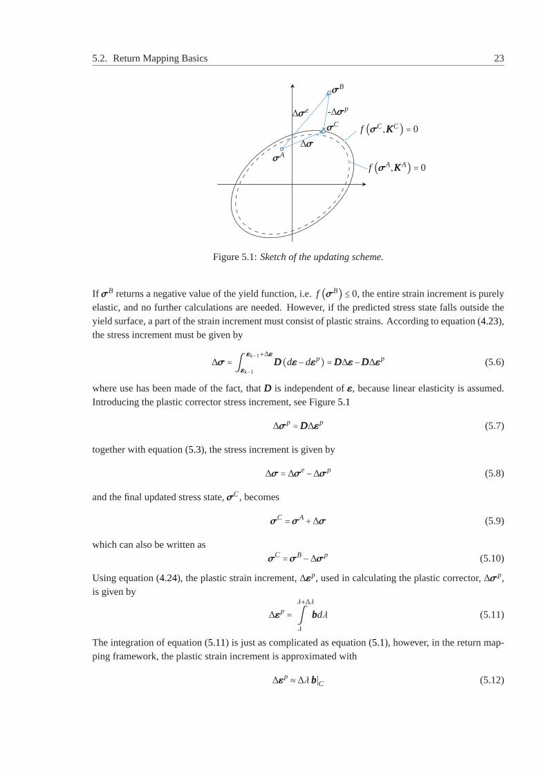
Figure 5.1:Sketch of the updating scheme.
If σσσB returns a negative value of the yield function, i.e.f (σσσB) ≤ 0, the entire strain increment is purelyelastic, and no further calculations are needed. However, if the predicted stress state falls outside theyield surface, a part of the strain increment must consist of plastic strains. According to equation (4.23),the stress increment must be given by
∆σσσ =∫ εεεk−1+∆εεε
εεεk−1
DDD(dεεε−dεεεp) =DDD∆εεε−DDD∆εεεp (5.6)
where use has been made of the fact, thatDDD is independent ofεεε, because linear elasticity is assumed.Introducing the plastic corrector stress increment, see Figure5.1
∆σσσp =DDD∆εεεp (5.7)
together with equation (5.3), the stress increment is given by
∆σσσ = ∆σσσe−∆σσσp (5.8)
and the final updated stress state,σσσC, becomes
σσσC =σσσA+∆σσσ (5.9)
which can also be written asσσσC =σσσB−∆σσσp (5.10)
Using equation (4.24), the plastic strain increment,∆εεεp, used in calculating the plastic corrector,∆σσσp,is given by
∆εεεp =λ+∆λ
∫λ
bbbdλ (5.11)
The integration of equation (5.11) is just as complicated as equation (5.1), however, in the return map-ping framework, the plastic strain increment is approximated with
∆εεεp ≈ ∆λ bbb∣C (5.12)
24 Chapter 5. Return Mapping in General Stress Space
which results in the plastic corrector increment,∆σσσp, can be written as
∆σσσp ≈ ∆λDDD bbb∣C (5.13)
and thus the problem boils down to finding the updated stress state,σσσC, which fulfills equation (5.10)and lies on the yield surface. If the updated stress state belongs to a single active yield function, cf.equation (4.24), the plastic corrector increment is given as shown above. However, ifthe updated stressstate belongs to an intersection of two or more yield functions, the plastic strain direction is given byequation (4.30). Because of this, slightly different return mapping procedures have to be deployed,depending on the number of active yield functions that the updated stress state,σσσC, belongs to.
5.3 Return to One Active Yield Function
The updated stress state,σσσC, belongs to the yield surface defined by the yield function hence
f (σσσC,KKKC) = 0 (5.14)
whereKKKC are the updated hardening variables
KKKC =KKK (κκκC) (5.15)
andκκκC are the updated state parameters. In case of a hardening law based upona potential function,this could be written as follows
κκκC = κκκA−∆λ ∂ j
∂KKK∣C
(5.16)
In order to find the correct updated stress state and the plastic multiplier, equation (5.10) and (5.14) aresolved using an iterative procedure, for instance a Newton-Raphson procedure, which is used in thistext.
5.3.1 Consistent Constitutive Matrix
DDDepc is derived by taking the total derivative of (5.8) with respect to∆εεε, using (5.3) and (5.13) as follows
d∆σσσ
d∆εεε= dDDD∆εεε
d∆εεε− ∂∆λDDDbbb
∂∆λ⋅ d∆λd∆εεε− ∂∆λDDDbbb
∂∆σσσ⋅ d∆σσσd∆εεε
(5.17)
Multiplying with d∆εεε on both sides yields
d∆σσσ =DDDd∆εεε−DDDbbbd∆λ−∆λDDD∂bbb
∂σσσd∆σσσ (5.18)
Rearranging leads to
d∆σσσ = (III +∆λDDD∂bbb
∂σσσ)−1
DDD(d∆εεε−d∆λbbb) (5.19)
which can be written on the formd∆σσσ =DDDcd∆εεε−d∆λDDDcbbb (5.20)
where
DDDc =TTTDDD (5.21)
TTT = (III +∆λDDD∂bbb
∂σσσ)−1
(5.22)
5.4. Return to Two Active Yield Functions 25
TTT is known as the modification matrix. Using the consistency condition, (4.22), an expression ford∆λcan be found in much the same way as it was found in (4.27), and substituted back into (5.20), whichgives the consistent constitutive matrix as
DDDepc=DDDc− DDDcbbbaaaTDDDc
aaaTDDDcbbb+( ∂ f∂KKK )
T∂KKK∂κκκ
∂ j∂KKK
(5.23)
If aaa is equal tobbb, it is seen, thatDDDepc is symmetric.
5.4 Return to Two Active Yield Functions
If the yield criterion consists of two yield functions,f1 and f2, with the appertaining plastic potentialsg1 andg2 and the hardening potentialsj1 and j2, it is possible, that the updated stress state belongs tothe intersection of these two yield surfaces, see Figure4.4. If this is the case, the direction of the plasticstrains is given by equation (4.30), and thus the corrector stress is also a linear combination of the stressdirections involved giving
∆σσσp = ∆λ1DDD bbb1∣C+∆λ2DDD bbb2∣C (5.24)
where
bbb1 = ∂g1
∂σσσ(5.25)
bbb2 = ∂g2
∂σσσ(5.26)
(5.27)
Similarly, the hardening law, equation (5.16) expands to
κκκC = κκκA−∆λ1∂ j1∂KKK∣C−∆λ2
∂ j2∂KKK∣C
(5.28)
when using the hardening potential method. The updated stress state belonging to the yield curve stillneeds to fulfill (5.10) as well asf1(σσσC,KKKC) =0 andf2(σσσC,KKKC) =0. This results in eight equations witheight unknowns, namelyσσσC, ∆λ1 and∆λ2. To find the updated stress state,σσσC, an iterative procedureis implemented in which the residual,rrr, of equation (5.10) is defined by
rrr (σσσC,∆λ1,∆λ2) =σσσC−(σσσB−∆λ1DDD bbb1∣C−∆λ2DDD bbb2∣C) =000 (5.29)
Expandingrrr in a first order Taylor series leads to
rrr (σσσCi+1,∆λ1,i+1,∆λ2,i+1) =rrr (σσσC
i +dσσσ,∆λ1,i +d∆λ1,∆λ2,i +d∆λ2)=rrr (σσσC
i ,∆λ1,i ,∆λ2,i)+ ∂rrr∂σσσ
dσσσ+ ∂rrr
∂∆λ1d∆λ1+ ∂rrr
∂∆λ2d∆λ2
(5.30)
where
∂rrr
∂σσσ= ∂σσσ
C
∂σσσ− ∂σσσB
∂σσσ+ ∂∆λ1DDDbbb1
∂σσσ+ ∂∆λ2DDDbbb2
∂σσσ(5.31)
= III +∆λ1DDD∂bbb1
∂σσσ+∆λ2DDD
∂bbb2
∂σσσ(5.32)
26 Chapter 5. Return Mapping in General Stress Space
and∂rrr
∂∆λ1=DDDbbb1 (5.33)
∂rrr
∂∆λ2=DDDbbb2 (5.34)
substituting back into (5.30) yields
rrr (σσσCi+1,∆λ1,i+1,∆λ2,i+1) =rrr (σσσC
i ,∆λ1,i ,∆λ2,i)+(III +∆λ1DDD∂bbb1
∂σσσ+∆λ2DDD
∂bbb2
∂σσσ)dσσσ+
+DDDbbb1 ⋅d∆λ1+DDDbbb2 ⋅d∆λ2
(5.35)
and solving forrrr (σσσCi+1,∆λ1,i+1,∆λ2,i+1) = 0 gives
dσσσ = (III +∆λ1DDD∂bbb1
∂σσσ+∆λ2DDD
∂bbb2
∂σσσ)−1
(−rrr (σσσCi ,∆λ1,i ,∆λ2,i)−DDDbbb1d∆λ2−DDDbbb2d∆λ2)
= −TTTrrr (σσσCi ,∆λ1,i ,∆λ2,i)−DDDcbbb1d∆λ2−DDDcbbb2d∆λ2
(5.36)
where
TTT = (III +∆λ1DDD∂bbb1
∂σσσ+∆λ2DDD
∂bbb2
∂σσσ)−1
(5.37)
Having an initial guess ofσσσCi , ∆λ1,i and∆λ2,i , a Taylor expansion of the two yield criteria results in
f1(σσσCi+1,KKK
Ci+1) = f1(σσσC
i +dσσσ,KKKCi +dKKK)
= f1(σσσCi ,KKK
Ci )+aaaT
1 dσσσ+(∂ f1∂KKK)
T
dKKK(5.38)
where
dKKK =∂KKK∂κκκ
∂κκκ
∂∆λ1d∆λ1+ ∂KKK
∂κκκ
∂κκκ
∂∆λ2d∆λ2
=− ∂KKK∂κκκ
∂ j1∂KKK
d∆λ1− ∂KKK∂κκκ
∂ j2∂KKK
d∆λ2 (5.39)
which gives
f1(σσσCi+1,KKK
Ci ) = f1(σσσC
i ,KKKCi+1)−aaaT
1TTTrrr (σσσCi ,∆λ1,i ,∆λ2,i)−aaaT
1DDDcbbb1d∆λ2−aaa1DDDcbbb2d∆λ2−
(∂ f1∂KKK)
T
(∂KKK∂κκκ
∂κκκ
∂∆λ1d∆λ1+ ∂KKK
∂κκκ
∂κκκ
∂∆λ2d∆λ2)
(5.40)
and similarly for f2
f2(σσσCi+1,KKK
Ci ) = f2(σσσC
i ,KKKCi+1)−aaaT
2TTTrrr (σσσCi ,∆λ1,i ,∆λ2,i)−aaaT
2DDDcbbb1d∆λ2−aaa2DDDcbbb2d∆λ2−
(∂ f2∂KKK)
T
(∂KKK∂κκκ
∂κκκ
∂∆λ1d∆λ1+ ∂KKK
∂κκκ
∂κκκ
∂∆λ2d∆λ2)
(5.41)
Equating (5.40) and (5.41) with 0, leads to two equations with two unknowns, namelyd∆λ1 andd∆λ2
which can be found. Onced∆λ1 andd∆λ2 are obtained,dσσσ can be found using (5.36), which leads toa newσσσC
i+1. Further∆λ1 and∆λ2 are updated by
∆λ1,i+1 = ∆λ1,i +d∆λ (5.42)
∆λ2,i+1 = ∆λ2,i +d∆λ (5.43)
And new values ofd∆λ1 andd∆λ2 can again be found. The above-mentioned steps are repeated untilsatisfactory precision is reached.
5.4.1. Consistent constitutive matrix 27
5.4.1 Consistent constitutive matrix
The consistent constitutive matrix of a point belonging to two active yield functions is found in much thesame was as it was found for the point belonging to one yield function, namelyby taking the derivativeof (5.8) and utilizing (5.24)
d∆σσσ
d∆εεε= dDDD∆εεε
d∆εεε− ∂∆λ1DDDbbb1
∂∆λ1⋅ d∆λ1
d∆εεε− ∂∆λ1DDDbbb1
∂∆σσσ⋅ d∆σσσd∆εεε− ∂∆λ2DDDbbb2
∂∆λ2⋅ d∆λ2
d∆εεε− ∂∆λ2DDDbbb2
∂∆σσσ⋅ d∆σσσd∆εεε
(5.44)
which can be rewritten tod∆σσσ =TTTDDD(d∆εεε−d∆λ1bbb1−d∆λ2bbb2) (5.45)
Using the consistency condition of both yield criteria together with equation (5.36) and (5.39), resultsin
aaaT1 d∆σσσ+(∂ f1
∂KKK)
T
dKKK =aaaT1TTTDDD(d∆εεε−d∆λ1bbb1−d∆λ2bbb2)−(∂ f1∂KKK)
T
(∂KKK∂κκκ
∂ j1∂KKK
d∆λ1+ ∂KKK∂κκκ
∂ j2∂KKK
d∆λ2) = 0
(5.46)
aaaT2 d∆σσσ+(∂ f1
∂KKK)
T
dKKK =aaaT2TTTDDD(d∆εεε−d∆λ1bbb1−d∆λ2bbb2)−(∂ f2∂KKK)
T
(∂KKK∂κκκ
∂ j1∂KKK
d∆λ1+ ∂KKK∂κκκ
∂ j2∂KKK
d∆λ2) = 0
(5.47)
This can also be written as ⎡⎢⎢⎢⎢⎣aaaT
1DDDc∆εεε
aaaT2DDDc∆εεε
⎤⎥⎥⎥⎥⎦−AAA⎡⎢⎢⎢⎢⎣dλ1
dλ2
⎤⎥⎥⎥⎥⎦=⎡⎢⎢⎢⎢⎣0
0
⎤⎥⎥⎥⎥⎦(5.48)
where
AAA=⎡⎢⎢⎢⎢⎣A11 A12
A21 A22
⎤⎥⎥⎥⎥⎦(5.49)
Aik =aaaTi DDDcbbbk+(∂ fi
∂KKK)T ∂KKK
∂κκκ
∂ jk∂KKK
(5.50)
Thus,dλ1 anddλ2 can be found to be
⎡⎢⎢⎢⎢⎣dλ1
dλ2
⎤⎥⎥⎥⎥⎦=BBB⎡⎢⎢⎢⎢⎣aaa1DDDcd∆εεε
aaa2DDDcd∆εεε
⎤⎥⎥⎥⎥⎦(5.51)
where
BBB=AAA−1 =⎡⎢⎢⎢⎢⎣B11 B12
B21 B22
⎤⎥⎥⎥⎥⎦(5.52)
Substituting back into (5.45) gives
d∆σσσ =DDDc(d∆εεε−B11aaaT1DDDcd∆εεεbbb1−B12aaa
T2DDDcd∆εεεbbb1
−B21aaaT1DDDcd∆εεεbbb2−B22aaa
T2DDDcd∆εεεbbb2) (5.53)
Using (5.53), DDDepc can be derived to
DDDepc=DDDc−B11bbb1aaaT1DDDc−B12bbb1aaa
T2DDDc−B21bbb2aaa
T1DDDc−B22bbb2aaa
T2DDDc (5.54)
28 Chapter 5. Return Mapping in General Stress Space
which can also be written as
DDDepc=DDDc− 2∑i=1
2∑j=1
Bi jbbbiaaaTj DDDc (5.55)
If needed, the infinitesimal constitutive matrix is found by replacingDDDc in (5.55) with DDD.
5.5 Return to Three Active Yield Functions
An updated stress state might also be returned to the intersection of three yieldsurfaces,f1, f2 and f3,with the plastic potentialsg1, g2 andg3 and the hardening potentialsj1, j2 and j3. This scenario is verysimilar to the scenario with two active yield surfaces, which was discussed in the previous section, andwill only be touched upon briefly. The plastic corrector is given by
∆σσσp = ∆λ1DDD bbb1∣C+∆λ2DDD bbb2∣C+∆λ3DDD bbb3∣C (5.56)
and the evolution law is assumed to be given by
κκκC = κκκA−∆λ1∂ j1∂KKK∣C−∆λ2
∂ j2∂KKK∣C−∆λ3
∂ j3∂KKK∣C
(5.57)
The return algorithm is almost identical to the one mentioned in the previous section, except that anextra unknown,∆λ3 needs to be found, which is possible because of the extra equation introducedby the consistency condition of the third yield criterion. The derivation of thisprocedure is omitted,however the modification matrix,TTT, is given by
TTT = (III +∆λ1DDD∂bbb1
∂σσσ+∆λ2DDD
∂bbb2
∂σσσ+∆λ3DDD
∂bbb3
∂σσσ)−1
(5.58)
Similarly, the consistent constitutive matrix can be found to be given by
DDDepc=DDDc− 3∑i=1
3∑j=1
Bi jbbbiaaaTj DDDc (5.59)
whereBBB is the 3×3 equivalent matrix to the one in the previous section.
5.6 Determination of Correct Return Type
In the general six-dimensional stress space, there is no easy way of determining, which of the abovementioned return algorithms, that should be applied to a certain predictor stress. Because of this, acommonly used strategy is to start out with returning to a single yield surface. The updated stress stateis then evaluated based upon some specific requirements. In case these requirements are not met, thepredictor stress is returned using a return to two yield surfaces and so on. In general stress space, it istheoretically possible, that an updated stress state has to be returned usingas much as six active yieldsurfaces. However, in the three dimensional principal stress space, geometric arguments can be applied,to establish which method is to be applied.
Chapter6
Return Mapping in Principal StressSpace
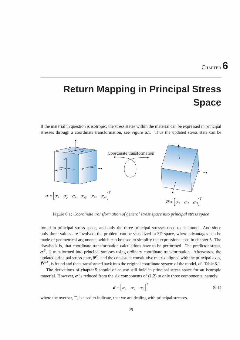
If the material in question is isotropic, the stress states within the material can be expressed in principalstresses through a coordinate transformation, see Figure6.1. Thus the updated stress state can be
σσσ = [σx σy σz σxy σxz σyz]Tσσσ = [σ1 σ2 σ3]T
Coordinate transformation
Figure 6.1:Coordinate transformation of general stress space into principal stressspace
found in principal stress space, and only the three principal stresses need to be found. And sinceonly three values are involved, the problem can be visualized in 3D space,where advantages can bemade of geometrical arguments, which can be used to simplify the expressionsused inchapter 5. Thedrawback is, that coordinate transformation calculations have to be performed. The predictor stress,σσσB, is transformed into principal stresses using ordinary coordinate transformation. Afterwards, theupdated principal stress state,σσσC, and the consistent constitutive matrix aligned with the principal axes,DDD
epc, is found and then transformed back into the original coordinate system ofthe model, cf. Table6.1.
The derivations ofchapter 5should of course still hold in principal stress space for an isotropicmaterial. However,σσσ is reduced from the six components of (1.2) to only three components, namely
σσσ = [σ1 σ2 σ3]T (6.1)
where the overbar, , is used to indicate, that we are dealing with principal stresses.
29
30 Chapter 6. Return Mapping in Principal Stress Space
○ σσσB→σσσB Transform predicted stress state into principal stresses
○ σσσC(σσσB) Find the updated principal stress state
○ DDDepc(σσσC) Find consistent constitutive matrix aligned with principal axes
○ σσσC→σσσC Transform updated principal stress state to general stresses
aligned with model axes
○ DDDepc→DDDepc Transform consistent constitutive matrix into general stresses
aligned with model axes
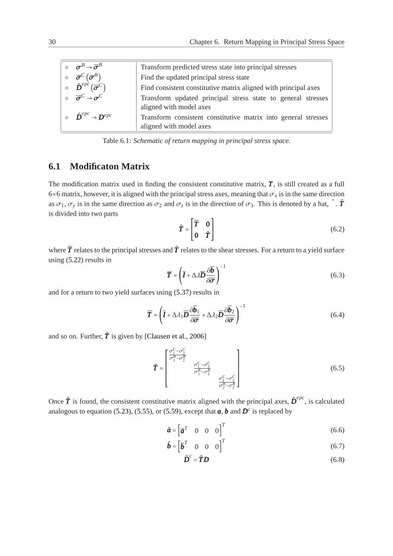
Table 6.1:Schematic of return mapping in principal stress space.
6.1 Modificaton Matrix
The modification matrix used in finding the consistent constitutive matrix,TTT, is still created as a full6×6 matrix, however, it is aligned with the principal stress axes, meaning thatσx is in the same directionasσ1, σy is in the same direction asσ2 andσz is in the direction ofσ3. This is denoted by a hat,ˆ . TTTis divided into two parts
TTT =⎡⎢⎢⎢⎢⎣TTT 000
000 TTT
⎤⎥⎥⎥⎥⎦(6.2)
whereTTT relates to the principal stresses andTTT relates to the shear stresses. For a return to a yield surfaceusing (5.22) results in
TTT = (III +∆λDDD∂bbb
∂σσσ)−1
(6.3)
and for a return to two yield surfaces using (5.37) results in
TTT = (III +∆λ1DDD∂bbb1
∂σσσ+∆λ2DDD
∂bbb2
∂σσσ)−1
(6.4)
and so on. Further,TTT is given by [Clausen et al., 2006]
TTT =⎡⎢⎢⎢⎢⎢⎢⎢⎢⎣
σC1−σ
C2
σB1−σ
B2
σC1−σ
C3
σB1−σ
B3
σC2−σ
C3
σB2−σ
B3
⎤⎥⎥⎥⎥⎥⎥⎥⎥⎦(6.5)
OnceTTT is found, the consistent constitutive matrix aligned with the principal axes,DDDepc
, is calculatedanalogous to equation (5.23), (5.55), or (5.59), except thataaa, bbb andDDDc is replaced by
aaa= [aaaT 0 0 0]T (6.6)
bbb= [bbbT0 0 0]T (6.7)
DDDc = TTTDDD (6.8)
6.2. Boundary Planes 31
6.2 Boundary Planes
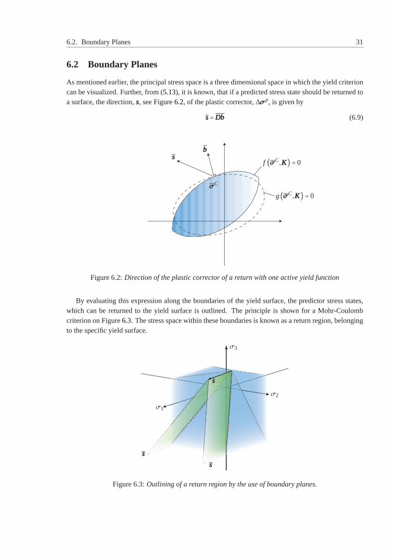
As mentioned earlier, the principal stress space is a three dimensional space in which the yield criterioncan be visualized. Further, from (5.13), it is known, that if a predicted stress state should be returned toa surface, the direction,sss, see Figure6.2, of the plastic corrector,∆σσσp, is given by
sss=DDDbbb (6.9)
sssbbb
f (σσσC,KKK) = 0
g(σσσC,KKK) = 0σσσC
Figure 6.2:Direction of the plastic corrector of a return with one active yield function
By evaluating this expression along the boundaries of the yield surface, the predictor stress states,which can be returned to the yield surface is outlined. The principle is shownfor a Mohr-Coulombcriterion on Figure6.3. The stress space within these boundaries is known as a return region, belongingto the specific yield surface.
σ1
σ2
σ3
sss
sss
sss
Figure 6.3:Outlining of a return region by the use of boundary planes.
32 Chapter 6. Return Mapping in Principal Stress Space
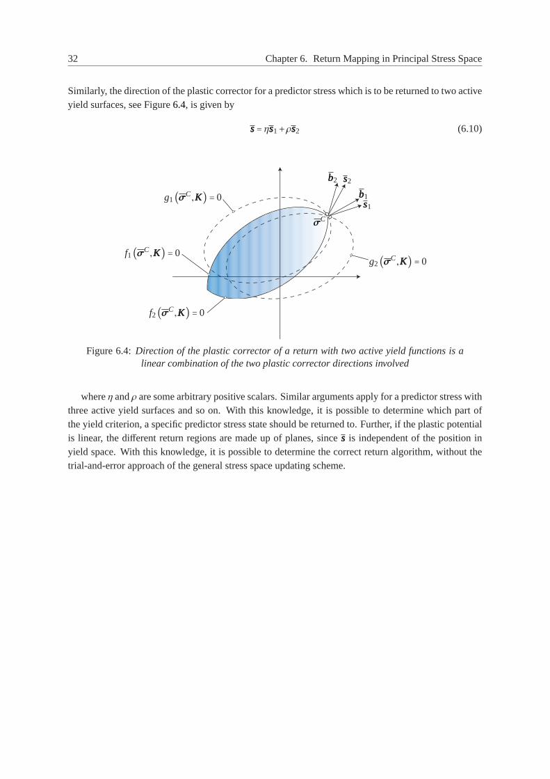
Similarly, the direction of the plastic corrector for a predictor stress which is tobe returned to two activeyield surfaces, see Figure6.4, is given by
sss= ηsss1+ρsss2 (6.10)
g1(σσσC,KKK) = 0
f1(σσσC,KKK) = 0g2(σσσC,KKK) = 0
f2(σσσC,KKK) = 0
bbb2
bbb1sss1
sss2
σσσC
Figure 6.4:Direction of the plastic corrector of a return with two active yield functions is alinear combination of the two plastic corrector directions involved
whereη andρ are some arbitrary positive scalars. Similar arguments apply for a predictorstress withthree active yield surfaces and so on. With this knowledge, it is possible to determine which part ofthe yield criterion, a specific predictor stress state should be returned to. Further, if the plastic potentialis linear, the different return regions are made up of planes, sincesss is independent of the position inyield space. With this knowledge, it is possible to determine the correct returnalgorithm, without thetrial-and-error approach of the general stress space updating scheme.
Chapter7
Implementation of Strain HardeningMohr-Coulomb Model
In this chapter, the theory of the previous chapters will be applied to a Mohr-Coulomb model usinglinear elasticity, non-associated plasticity and isotropic strain hardening, along with the evolution lawsof equation (4.25) and (4.31).
7.1 Basic Premises
As mentioned inchapter 3, the Mohr-Coulomb yield criterion can take the form of
f (σσσ,σc,k) = kσ1−σ3−σc = 0 (7.1)
which will be used in the current implementation due to its simplicity compared to (3.5). The yieldcriterion is a function of both the friction angle,ϕ, and the cohesionc. In this implementation, it isassumed, that the friction angle remains constant. Thus, the hardening parameters vector,KKK, simplifiesto a scalar, namely the cohesion,c. Further the state parameters vector,κκκ, of the material, is chosen tobe the scalar accumulated plastic strain, ¯εP. Thus
KKK (κκκ) = c(εP) (7.2)
The plastic potential,g, is chosen as
g= (σσσ,c,ψ) =σ1−σ3+(σ1+σ3)sin(ψ)−2ccos(ψ) (7.3)
whereψ represents the angle of dilation. The evolution of the accumulated plastic strainis given by thehardening potential function,j, cf. equation (4.25), and is chosen as
j = (σσσ,c,ϕ) =σ1−σ3+(σ1+σ3)sin(ϕ)−2ccos(ϕ) (7.4)
7.2 Derivatives
The derivative off with respect toσσσ is given by
aaa= ∂ f
∂σσσ=⎡⎢⎢⎢⎢⎢⎢⎣
k
0
−1
⎤⎥⎥⎥⎥⎥⎥⎦(7.5)
33
34 Chapter 7. Implementation of Strain Hardening Mohr-Coulomb Model
The derivative off with respect to the harding variable,c, is given by
∂ f
∂KKK= ∂ f
∂c= ∂ f
∂σc
dσc
dc= −2√
k (7.6)
The derivative ofg with respect toσσσ is given by
bbb= ∂g
∂σσσ=⎡⎢⎢⎢⎢⎢⎢⎣
1+sin(ψ)0
−1+sin(ψ)
⎤⎥⎥⎥⎥⎥⎥⎦(7.7)
The derivative ofj with respect to the hardening variables is given by
∂ j
∂KKK= ∂ j
∂c= −2cos(ϕ) (7.8)
Finally, the derivative of the hardening parameters,KKK, with respect to the state parameters,κκκ, is givenby
∂KKK
∂κκκ= ∂c
∂εP= H (7.9)
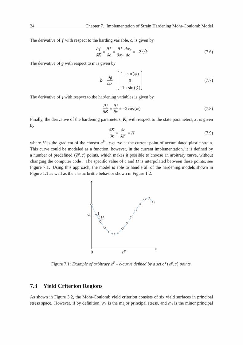
whereH is the gradient of the chosen ¯εP−c-curve at the current point of accumulated plastic strain.This curve could be modeled as a function, however, in the current implementation, it is defined bya number of predefined(εp,c) points, which makes it possible to choose an arbitrary curve, withoutchanging the computer code . The specific value ofc andH is interpolated between these points, seeFigure7.1. Using this approach, the model is able to handle all of the hardening models shown inFigure1.1as well as the elastic brittle behavior shown in Figure1.2.
c
0 εp
1H
Figure 7.1:Example of arbitraryεP−c-curve defined by a set of(εp,c) points.
7.3 Yield Criterion Regions
As shown in Figure3.2, the Mohr-Coulomb yield criterion consists of six yield surfaces in principalstress space. However, if by definition,σ1 is the major principal stress, andσ3 is the minor principal
7.3. Yield Criterion Regions 35
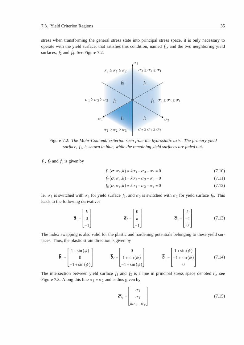
stress when transforming the general stress state into principal stress space, it is only necessary tooperate with the yield surface, that satisfies this condition, namedf1, and the two neighboring yieldsurfaces,f2 and f6. See Figure7.2.
f1 f2
f3
f4f5
f6
σ1 ≥σ2 ≥σ3 σ2 ≥σ1 ≥σ3
σ2 ≥σ3 ≥σ1
σ3 ≥σ2 ≥σ1σ3 ≥σ1 ≥σ2
σ1 ≥σ3 ≥σ2
σ1 σ2
σ3
Figure 7.2:The Mohr-Coulomb criterion seen from the hydrostatic axis. The primary yieldsurface, f1, is shown in blue, while the remaining yield surfaces are faded out.
f1, f2 and f6 is given by
f1(σσσ,σc,k) = kσ1−σ3−σc = 0 (7.10)
f2(σσσ,σc,k) = kσ2−σ3−σc = 0 (7.11)
f6(σσσ,σc,k) = kσ1−σ2−σc = 0 (7.12)
Ie. σ1 is switched withσ2 for yield surfacef2, andσ3 is switched withσ2 for yield surfacef6. Thisleads to the following derivatives
aaa1 =⎡⎢⎢⎢⎢⎢⎢⎣
k
0
−1
⎤⎥⎥⎥⎥⎥⎥⎦aaa2 =⎡⎢⎢⎢⎢⎢⎢⎣
0
k
−1
⎤⎥⎥⎥⎥⎥⎥⎦aaa6 =⎡⎢⎢⎢⎢⎢⎢⎣
k
−1
0
⎤⎥⎥⎥⎥⎥⎥⎦(7.13)
The index swapping is also valid for the plastic and hardening potentials belonging to these yield sur-faces. Thus, the plastic strain direction is given by
bbb1 =⎡⎢⎢⎢⎢⎢⎢⎣
1+sin(ψ)0
−1+sin(ψ)
⎤⎥⎥⎥⎥⎥⎥⎦bbb2 =⎡⎢⎢⎢⎢⎢⎢⎣
0
1+sin(ψ)−1+sin(ψ)
⎤⎥⎥⎥⎥⎥⎥⎦bbb6 =⎡⎢⎢⎢⎢⎢⎢⎣
1+sin(ψ)−1+sin(ψ)
0
⎤⎥⎥⎥⎥⎥⎥⎦(7.14)
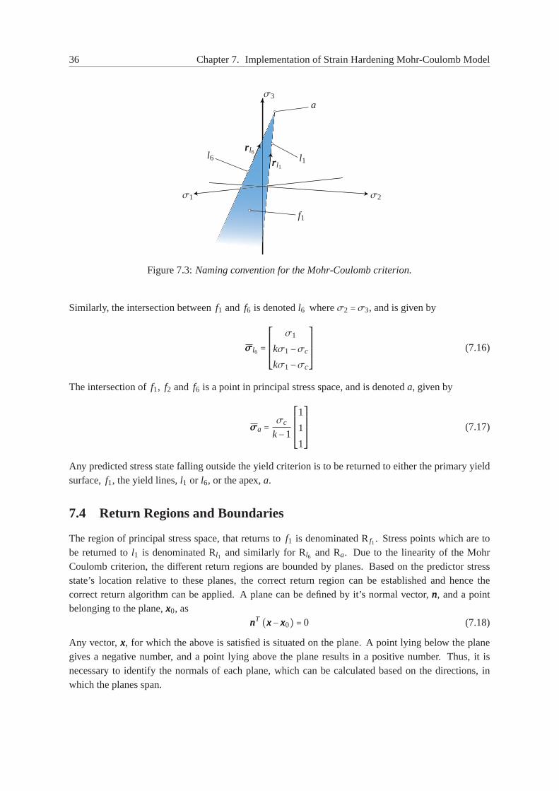
The intersection between yield surfacef1 and f2 is a line in principal stress space denotedl1, seeFigure7.3. Along this lineσ1 =σ2 and is thus given by
σσσl1 =⎡⎢⎢⎢⎢⎢⎢⎣
σ1
σ1
kσ1−σc
⎤⎥⎥⎥⎥⎥⎥⎦(7.15)
36 Chapter 7. Implementation of Strain Hardening Mohr-Coulomb Model
σ1 σ2
σ3a
l1l6
f1
rrr l1
rrr l6
Figure 7.3:Naming convention for the Mohr-Coulomb criterion.
Similarly, the intersection betweenf1 and f6 is denotedl6 whereσ2 =σ3, and is given by
σσσl6 =⎡⎢⎢⎢⎢⎢⎢⎣
σ1
kσ1−σc
kσ1−σc
⎤⎥⎥⎥⎥⎥⎥⎦(7.16)
The intersection off1, f2 and f6 is a point in principal stress space, and is denoteda, given by
σσσa = σc
k−1
⎡⎢⎢⎢⎢⎢⎢⎣
1
1
1
⎤⎥⎥⎥⎥⎥⎥⎦(7.17)
Any predicted stress state falling outside the yield criterion is to be returned to either the primary yieldsurface,f1, the yield lines,l1 or l6, or the apex,a.
7.4 Return Regions and Boundaries
The region of principal stress space, that returns tof1 is denominated Rf1. Stress points which are tobe returned tol1 is denominated Rl1 and similarly for Rl6 and Ra. Due to the linearity of the MohrCoulomb criterion, the different return regions are bounded by planes. Based on the predictor stressstate’s location relative to these planes, the correct return region can beestablished and hence thecorrect return algorithm can be applied. A plane can be defined by it’s normal vector,nnn, and a pointbelonging to the plane,xxx0, as
nnnT (xxx−xxx0) = 0 (7.18)
Any vector,xxx, for which the above is satisfied is situated on the plane. A point lying below theplanegives a negative number, and a point lying above the plane results in a positive number. Thus, it isnecessary to identify the normals of each plane, which can be calculated based on the directions, inwhich the planes span.
7.4. Return Regions and Boundaries 37
The plastic corrector direction belonging to a surface return to yield surface f1 is given by
sss1 =DDDbbb1 = − E
(1+ν)(2ν−1)⎡⎢⎢⎢⎢⎢⎢⎣
1+sin(ϕ)−2ν
2νsin(ϕ)2ν−1+sin(ϕ)
⎤⎥⎥⎥⎥⎥⎥⎦(7.19)
and the intersection between thef1-yield surface and thef2-yield surface is fully determined byσσσl1,(7.15), which by differentiation gives the direction of the intersection line,rrr l1, see Figure7.3,
rrr l1 = ∂σσσl1
∂σ1=⎡⎢⎢⎢⎢⎢⎢⎣
1
1
k
⎤⎥⎥⎥⎥⎥⎥⎦(7.20)
By taking the cross product betweenrrr l1 andsss1, the normal of the plane separating the return regionbelonging to yield surfacef1, and those belonging to linel1can be established as
nnnRf1→Rl1= sss1×rrr l1 (7.21)
where the arrow designates, that the normal of the plane is pointing from theregion belonging tof1, tothe region belonging tol1. Similarly, the direction ofl6 is given by
rrr l6 = ∂σσσl6
∂σ1=⎡⎢⎢⎢⎢⎢⎢⎣
1
k
k
⎤⎥⎥⎥⎥⎥⎥⎦(7.22)
and thus the normal of the plane which creates the boundary between the region of predictor stressesbelonging tof1 and those belonging tol6 can be found to give
nnnRl6→Rf1= sss1 ×rrr l6 (7.23)
The boundary plane separating Rl1 from Ra is spanned by the direction ofsss1 andsss2, which is the plasticcorrector direction belonging tof2. Thus
nnnRl1→Ra = sss1×sss2 (7.24)
and similarly for the boundary plane which separates Rl6 from Ra
nnnRl6→Ra = sss6×sss1 (7.25)
In order to completely define the boundary planes, a point on each plane isalso needed. Since all theplanes go through the apex of the criterion, this point is simply chosen to represent all four boundaryplanes. Based upon this, four boundary planes, see Figure7.4, can be defined by
pRf1→Rl1(σσσB) =nnnT
Rf1→Rl1(σσσB−σσσa) = 0 (7.26)
pRl6→Rf1(σσσB) =nnnT
Rl6→Rf1(σσσB−σσσa) = 0 (7.27)
pRl1→Ra (σσσB) =nnnTRl1→Ra
(σσσB−σσσa) = 0 (7.28)
pRl6→Ra (σσσB) =nnnT
Rl6→Ra(σσσB−σσσa) = 0 (7.29)
Using these boundary planes, a rule set can be set up, which determinesthe correct return algorithmbased upon the evaluation of these planes, which has been done in Table7.1.
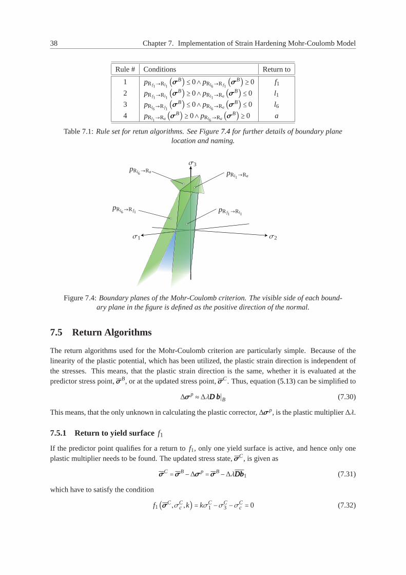
38 Chapter 7. Implementation of Strain Hardening Mohr-Coulomb Model
Rule # Conditions Return to
1 pRf1→Rl1(σσσB) ≤ 0∧ pRl6
→Rf1(σσσB) ≥ 0 f1
2 pRf1→Rl1(σσσB) ≥ 0∧ pRl1→Ra (σσσB) ≤ 0 l1
3 pRl6→Rf1(σσσB) ≤ 0∧ pRl6
→Ra (σσσB) ≤ 0 l64 pRl1→Ra (σσσB) ≥ 0∧ pRl6
→Ra (σσσB) ≥ 0 a
Table 7.1:Rule set for retun algorithms. See Figure7.4 for further details of boundary planelocation and naming.
σ1 σ2
σ3
pRl1→Ra
pRf1→Rl1
pRl6→Ra
pRl6→Rf1
Figure 7.4:Boundary planes of the Mohr-Coulomb criterion. The visible side of eachbound-ary plane in the figure is defined as the positive direction of the normal.
7.5 Return Algorithms
The return algorithms used for the Mohr-Coulomb criterion are particularly simple. Because of thelinearity of the plastic potential, which has been utilized, the plastic strain directionis independent ofthe stresses. This means, that the plastic strain direction is the same, whether itis evaluated at thepredictor stress point,σσσB, or at the updated stress point,σσσC. Thus, equation (5.13) can be simplified to
∆σσσp ≈ ∆λDDD bbb∣B (7.30)
This means, that the only unknown in calculating the plastic corrector,∆σσσp, is the plastic multiplier∆λ.
7.5.1 Return to yield surfacef1
If the predictor point qualifies for a return tof1, only one yield surface is active, and hence only oneplastic multiplier needs to be found. The updated stress state,σσσC, is given as
σσσC =σσσB−∆σσσp =σσσB−∆λDDDbbb1 (7.31)
which have to satisfy the condition
f1(σσσC,σCc ,k) = kσC
1 −σC3 −σC
c = 0 (7.32)
7.5.2. Return to yield linesl1 andl6 39
With the use of equation (7.31), σC1 andσC
3 can be expressed as
σC1 =σB
1 −∆λs1,1 (7.33)
σC3 =σB
3 −∆λs1,3 (7.34)
wheres1,1 ands1,3 is the first and third component ofsss1 respectively. Further, with the use of equation(5.16), the uniaxial compressive strength of the updated stress state,σC
c , depends on the accumulatedplastic strain at the updated stress state,εp,C, which is given as
εp,C = εp,A−∆λ∂ j
∂c= εp,A+∆λ2cos(ϕ) (7.35)
where equation (7.8) has been used. Thus, the compressive uniaxial strength of the updated stress state,σC
c , is given byσC
c = 2c(εp,C) √k (7.36)
Substituting back into equation (7.32) gives
f1(∆λ) = k(σB1 −∆λs1,1)−(σB
3 −∆λs1,3)−σCc = 0 (7.37)
which is solved using an ordinary Newton-Raphson iteration procedure with respect to∆λ. The gradientof the equation with respect to∆λ is
d f1d∆λ
= −ks1,1+ s1,3− dσCc
dcC
dcC
dεp,C
dεp,C
d∆λ= −ks1,1+ s1,3+dσc (7.38)
where
dσc = −dσCc
dcC
dcC
dεp,C
dεp,C
d∆λ= 4H cos(ϕ) √k (7.39)
using equation (7.9), (7.35) and (7.36). An initial guess of∆λ is made and then updated via
∆λi+1 = ∆λi −( d f1d∆λ∣i)−1
f1(∆λi) (7.40)
until the required precision is reached.
7.5.2 Return to yield linesl1 and l6
Returning to one of the yield lines,l1 and l6 is a simple expansion of the procedure used for thef1return. However, in this case, the plastic corrector is given by
σσσC =σσσB−∆σσσp =σσσB−∆λ1DDDbbb1−∆λ1DDDbbb2 (7.41)
where∆λ1 and∆λ2 are unknown.σσσC has to fulfill both yield criteria. For thel1 return, this results in
f1(σσσC,σCc ,k) = kσC
1 −σC3 −σC
c = 0 (7.42)
f2(σσσC,σCc ,k) = kσC
2 −σC3 −σC
c = 0 (7.43)
where
σC1 =σB
1 −∆λ1s1,1−∆λ2s2,1 (7.44)
σC2 =σB
2 −∆λ1s1,2−∆λ2s2,2 (7.45)
σC3 =σB
3 −∆λ1s1,3−∆λ2s2,3 (7.46)
40 Chapter 7. Implementation of Strain Hardening Mohr-Coulomb Model
The accumulated plastic strain of the updated stress state is given by
εp,C = εp,A− 2∑i=1∆λi
∂ j i∂c= εp,A−2cos(ϕ)(∆λ1+∆λ2) (7.47)
The two yield criteria are embedded in the residual vectorFFF as
FFF (∆λλλ) =⎡⎢⎢⎢⎢⎣
f1(∆λ1,∆λ2)f2(∆λ1,∆λ2)
⎤⎥⎥⎥⎥⎦=⎡⎢⎢⎢⎢⎣k(σB
1 −∆λ1s1,1−∆λ2s2,1)−(σB3 −∆λ1s1,3−∆λ2s2,3)−σC
c
k(σB2 −∆λ1s1,2−∆λ2s2,2)−(σB
3 −∆λ1s1,3−∆λ2s2,3)−σCc
⎤⎥⎥⎥⎥⎦=⎡⎢⎢⎢⎢⎣0
0
⎤⎥⎥⎥⎥⎦(7.48)
where
∆λλλ =⎡⎢⎢⎢⎢⎣∆λ1
∆λ2
⎤⎥⎥⎥⎥⎦(7.49)
The gradient is found to be
∂FFF
∂∆λλλT=⎡⎢⎢⎢⎢⎣−ks1,1+ s1,3+dσc −ks2,1+ s2,3+dσc
−ks1,2+ s1,3+dσc −ks2,2+ s2,3+dσc
⎤⎥⎥⎥⎥⎦(7.50)
wheredσc is given by (7.39). The system of equations is solved using a Newton-Raphson iteration,where an initial guess of∆λλλ is made, an afterwards updated as
∆λλλi+1 = ∆λλλi −( ∂FFF
∂∆λλλT∣i)−1
FFF (∆λλλi) (7.51)
until the required precision is reached. The return algorithm for thel6 return is analogous to the above,except that thef2 yield surface is replaced by thef6 yield surface. This gives
FFF (∆λλλ) =⎡⎢⎢⎢⎢⎣
f1(∆λ1,∆λ2)f6(∆λ1,∆λ2)
⎤⎥⎥⎥⎥⎦=⎡⎢⎢⎢⎢⎣k(σB
1 −∆λ1s1,1−∆λ2s2,1)−(σB3 −∆λ1s1,3−∆λ2s2,3)−σC
c
k(σB1 −∆λ1s1,1−∆λ2s2,1)−(σB
2 −∆λ1s1,2−∆λ2s2,2)−σCc
⎤⎥⎥⎥⎥⎦=⎡⎢⎢⎢⎢⎣0
0
⎤⎥⎥⎥⎥⎦(7.52)
with the corresponding gradient
∂FFF
∂∆λλλT=⎡⎢⎢⎢⎢⎣−ks1,1+ s1,3+dσc −ks2,1+ s2,3+dσc
−ks1,1+ s1,2+dσc −ks2,1+ s2,2+dσc
⎤⎥⎥⎥⎥⎦(7.53)
7.5.3 Return to apex pointa
The return algorithm to the apex of the Mohr-Coulomb criterion is a further expansion of thel1 andl6algorithms, in which casef1, f2 and f3 needs to be fulfilled. The approach is similar to the above and
7.6. Consistent Constitutive Matrix 41
only the main results will be given here. The residual vector is found to be given by
FFF (∆λλλ) =⎡⎢⎢⎢⎢⎢⎢⎣
f1(∆λ1,∆λ2,∆λ3)f2(∆λ1,∆λ2,∆λ3)f6(∆λ1,∆λ2,∆λ3)
⎤⎥⎥⎥⎥⎥⎥⎦=⎡⎢⎢⎢⎢⎢⎢⎣
k(σB1 −∆λ1s1,1−∆λ2s2,1−∆λ3s3,1)−(σB
3 −∆λ1s1,3−∆λ2s2,3−∆λ3s3,3)−σCc
k(σB2 −∆λ1s1,2−∆λ2s2,2−∆λ3s3,2)−(σB
3 −∆λ1s1,3−∆λ2s2,3−∆λ3s3,3)−σCc
k(σB1 −∆λ1s1,1−∆λ2s2,1−∆λ3s3,1)−(σB
2 −∆λ1s1,2−∆λ2s2,2−∆λ3s3,2)−σCc
⎤⎥⎥⎥⎥⎥⎥⎦=⎡⎢⎢⎢⎢⎢⎢⎣
0
0
0
⎤⎥⎥⎥⎥⎥⎥⎦
(7.54)
where
∆λλλ =⎡⎢⎢⎢⎢⎢⎢⎣
∆λ1
∆λ2
∆λ3
⎤⎥⎥⎥⎥⎥⎥⎦(7.55)
and the gradient matrix is given by
∂FFF
∂∆λλλT=⎡⎢⎢⎢⎢⎢⎢⎣
−ks1,1+ s1,3+dσc −ks2,1+ s2,3+dσc −ks3,1+ s3,3+dσc
−ks1,2+ s1,3+dσc −ks2,2+ s2,3+dσc −ks3,2+ s3,3+dσc
−ks1,1+ s1,2+dσc −ks2,1+ s2,2+dσc −ks3,1+ s3,2+dσc
⎤⎥⎥⎥⎥⎥⎥⎦(7.56)
7.6 Consistent Constitutive Matrix
In the evaluation of the consistent constitutive matrix, the modification matrix aligned with the principalstresses,TTT is needed. The part related to the principal stresses,TTT, see equation (6.3), simplifies to theunit matrix
TTT =⎡⎢⎢⎢⎢⎢⎢⎣
1 0 0
0 1 0
0 0 1
⎤⎥⎥⎥⎥⎥⎥⎦(7.57)
because the derivative ofbbb with respect toσσσ results in the zero-matrix
∂bbb
∂σσσ=⎡⎢⎢⎢⎢⎢⎢⎣
0 0 0
0 0 0
0 0 0
⎤⎥⎥⎥⎥⎥⎥⎦(7.58)
The part ofTTT, that relates to the shear stresses,TTT, is simply evaluated by equation (6.5). Thus it ispossible to evaluateDDD
c. Afterwards, the consistent constitutive matrix aligned with the principal axes,
DDDepc
, is calculated using either equation (5.23), (5.55) or (5.59), depending on the return algorithm usedin finding the updated stress state.

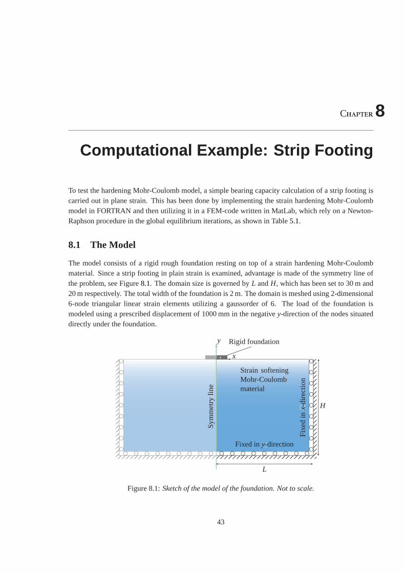
Chapter8
Computational Example: Strip Footing
To test the hardening Mohr-Coulomb model, a simple bearing capacity calculation of a strip footing iscarried out in plane strain. This has been done by implementing the strain hardening Mohr-Coulombmodel in FORTRAN and then utilizing it in a FEM-code written in MatLab, which relyon a Newton-Raphson procedure in the global equilibrium iterations, as shown in Table5.1.
8.1 The Model
The model consists of a rigid rough foundation resting on top of a strain hardening Mohr-Coulombmaterial. Since a strip footing in plain strain is examined, advantage is made of the symmetry line ofthe problem, see Figure8.1. The domain size is governed byL andH, which has been set to 30 m and20 m respectively. The total width of the foundation is 2 m. The domain is meshedusing 2-dimensional6-node triangular linear strain elements utilizing a gaussorder of 6. The loadof the foundation ismodeled using a prescribed displacement of 1000 mm in the negativey-direction of the nodes situateddirectly under the foundation.
Sym
met
rylin
e
Rigid foundation
Fix
edin
x-di
rect
ion
Fixed iny-direction
Strain softeningMohr-Coulombmaterial
H
L
x
y
Figure 8.1:Sketch of the model of the foundation. Not to scale.
43
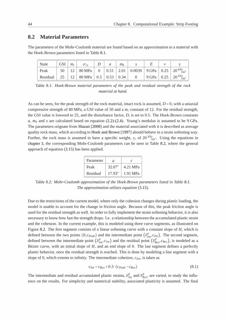
44 Chapter 8. Computational Example: Strip Footing
8.2 Material Parameters
The parameters of the Mohr-Coulomb material are found based on an approximation to a material withthe Hoek-Brown parameters listed in Table8.1.
State GSI mi σci D a mb s E ν γ
Peak 50 12 80 MPa 0 0.51 2.01 0.0039 9 GPa 0.25 20kN/m3
Residual 25 12 80 MPa 0.5 0.53 0.34 0 9 GPa 0.25 20kN/m2
Table 8.1: Hoek-Brown material parameters of the peak and residual strength ofthe rockmaterial at hand.
As can be seen, for the peak strength of the rock material, intact rock is assumed,D = 0, with a uniaxialcompressive strength of 80 MPa, a GSI value of 50 and ami constant of 12. For the residual strength,the GSI value is lowered to 25, and the disturbance factor,D, is set to 0.5. The Hoek-Brown constantsa, mb and s are calculated based on equation (2.2)-(2.4). Young’s modulus is assumed to be 9 GPa.The parameters orignate fromSharan[2008] and the material associated with it is described as averagequality rock mass, which according toHoek and Brown[1997] should behave in a strain softening way.Further, the rock mass is assumed to have a specific weight,γ, of 20kN/m3. Using the equations inchapter 3, the corresponding Mohr-Coulomb parameters can be seen in Table8.2, where the generalapproach of equation (3.15) has been applied.
Parameter ϕ c
Peak 32.07○ 4.21 MPa
Residual 17.93○ 1.91 MPa
Table 8.2:Mohr-Coulomb approximation of the Hoek-Brown parameters listed in Table 8.1.The approximation utilizes equation(3.15).
Due to the restrictions of the current model, where only the cohesion changes during plastic loading, themodel is unable to account for the change in friction angle. Because of this, the peak friction angle isused for the residual strength as well. In order to fully implement the strain softening behavior, it is alsonecessary to know how fast the strength drops. I.e. a relationship between the accumulated plastic strainand the cohesion. In the current example, this is modeled using three curvesegments, as illustrated onFigure8.2. The first segment consists of a linear softening curve with a constant slope ofH, which isdefined between the two points(0,cPeak) and the intermediate point(εp
Int,cInt). The second segment,defined between the intermediate point(εp
Int,cInt) and the residual point(εpRes,cRes), is modeled as a
Bézier curve, with an initial slope ofH, and an end slope of 0. The last segment defines a perfectlyplastic behavior, once the residual strength is reached. This is done by modeling a line segment with aslope of 0, which extents to infinity. The intermediate cohesion,cInt, is taken as
cInt = cRes+0.3 ⋅ (cPeak−cRes) (8.1)
The intermediate and residual accumulated plastic strains,εpInt andεp
Res, are varied, to study the influ-ence on the results. For simplicity and numerical stability, associated plasticity is assumed. The final
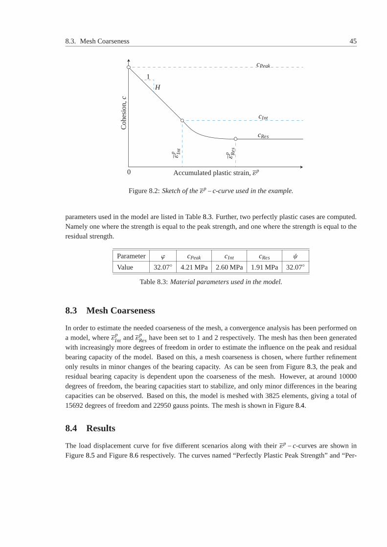
8.3. Mesh Coarseness 45
Coh
esio
n,c
cPeak
cInt
cRes
Accumulated plastic strain,εpε
p Int
εp R
es
0
1
H
Figure 8.2:Sketch of theεp−c-curve used in the example.
parameters used in the model are listed in Table8.3. Further, two perfectly plastic cases are computed.Namely one where the strength is equal to the peak strength, and one wherethe strength is equal to theresidual strength.
Parameter ϕ cPeak cInt cRes ψ
Value 32.07○ 4.21 MPa 2.60 MPa 1.91 MPa 32.07○
Table 8.3:Material parameters used in the model.
8.3 Mesh Coarseness
In order to estimate the needed coarseness of the mesh, a convergence analysis has been performed ona model, whereεp
Int andεpReshave been set to 1 and 2 respectively. The mesh has then been generated
with increasingly more degrees of freedom in order to estimate the influence on the peak and residualbearing capacity of the model. Based on this, a mesh coarseness is chosen, where further refinementonly results in minor changes of the bearing capacity. As can be seen fromFigure8.3, the peak andresidual bearing capacity is dependent upon the coarseness of the mesh. However, at around 10000degrees of freedom, the bearing capacities start to stabilize, and only minordifferences in the bearingcapacities can be observed. Based on this, the model is meshed with 3825 elements, giving a total of15692 degrees of freedom and 22950 gauss points. The mesh is shownin Figure8.4.
8.4 Results
The load displacement curve for five different scenarios along with theirεp− c-curves are shown inFigure8.5 and Figure8.6 respectively. The curves named “Perfectly Plastic Peak Strength” and “Per-
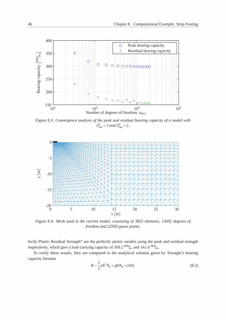
46 Chapter 8. Computational Example: Strip Footing
Number of degrees of freedom,ndo f
Bea
ring
capa
city
,[MN/ m]
Peak bearing capacityResidual bearing capacity
102 103 104 105150
200
250
300
350
400
Figure 8.3:Convergence analysis of the peak and residual bearing capacity of a model withε
pInt = 1 andεp
Int = 2.
x [m]
y[m]
0 5 10 15 20 25 30-20
-15
-10
-5
0
Figure 8.4:Mesh used in the current model, consisting of 3825 elements, 15692 degrees offreedom and 22950 gauss points.
fectly Plastic Residual Strength” are the perfectly plastic models using the peak and residual strengthrespectively, which give a load carrying capacity of 309.2 MN/m and 141.6 MN/m.
To verify these results, they are compared to the analytical solution given by Terzaghi’s bearingcapacity formula
R= 12γb2Nγ+qbNq+cbNc (8.2)
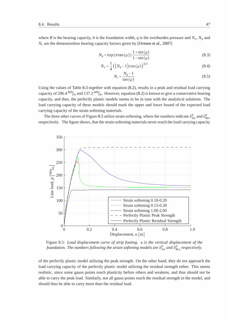
8.4. Results 47
whereR is the bearing capacity,b is the foundation width,q is the overburden pressure andNγ, Nq andNc are the dimensionless bearing capacity factors given by [Ovesen et al., 2007]
Nq = exp(π tan(ϕ))1+sin(ϕ)1−sin(ϕ)
(8.3)
Nγ = 14((Nq−1)cos(ϕ))3/2 (8.4)
Nc = Nq−1
tan(ϕ)(8.5)
Using the values of Table8.3 together with equation (8.2), results in a peak and residual load carryingcapacity of 296.4MN/m and 137.2MN/m. However, equation (8.2) is known to give a conservative bearingcapacity, and thus, the perfectly plastic models seems to be in tune with the analytical solutions. Theload carrying capacity of these models should mark the upper and lower bound of the expected loadcarrying capacity of the strain softening materials.
The three other curves of Figure8.5utilize strain softening, where the numbers indicateεpInt andεp
Res
respectively. The figure shows, that the strain softening materials neverreach the load carrying capacity
Displacement,u [m]
Line
load
,p[M
N/ m]
Perfectly Plastic Peak StrengthPerfectly Plastic Residual Strength
Strain softening 0.10-0.20Strain softening 0.15-0.30Strain softening 1.00-2.00
00 0.2 0.4 0.6 0.8 1.0
50
100
150
200
250
300
350
Figure 8.5: Load displacement curve of strip footing. u is the vertical displacement ofthefoundation. The numbers following the strain softening models areε
pInt andεp
Resrespectively.
of the perfectly plastic model utilizing the peak strength. On the other hand, they do not approach theload carrying capacity of the perfectly plastic model utilizing the residual strength either. This seemsrealistic, since some gauss points reach plasticity before others and weakens, and thus should not beable to carry the peak load. Similarly, not all gauss points reach the residual strength in the model, andshould thus be able to carry more than the residual load.
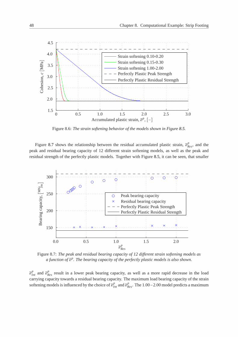
48 Chapter 8. Computational Example: Strip Footing
Accumulated plastic strain,εp, [−]
Coh
esio
n,c[M
Pa]
Perfectly Plastic Peak Strength
Perfectly Plastic Residual Strength
Strain softening 0.10-0.20Strain softening 0.15-0.30Strain softening 1.00-2.00
0 0.5 1.0 1.5 2.0 2.5 3.01.5
2.0
2.5
3.0
3.5
4.0
4.5
Figure 8.6:The strain softening behavior of the models shown in Figure8.5.
Figure 8.7 shows the relationship between the residual accumulated plastic strain,εpRes, and the
peak and residual bearing capacity of 12 different strain softening models, as well as the peak andresidual strength of the perfectly plastic models. Together with Figure8.5, it can be seen, that smaller
εpRes
Bea
ring
capa
city
,[MN/ m]
Peak bearing capacityResidual bearing capacity
Perfectly Plastic Residual StrengthPerfectly Plastic Peak Strength
0.0 0.5 1.0 1.5 2.0
150
200
250
300
Figure 8.7:The peak and residual bearing capacity of 12 different strain softening models asa function ofεp. The bearing capacity of the perfectly plastic models is also shown.
εpInt and εp
Res result in a lower peak bearing capacity, as well as a more rapid decreasein the loadcarrying capacity towards a residual bearing capacity. The maximum load bearing capacity of the strainsoftening models is influenced by the choice ofε
pInt andεp
Res. The 1.00−2.00 model predicts a maximum
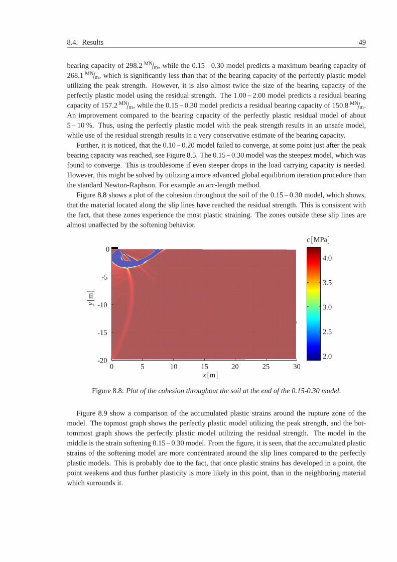
8.4. Results 49
bearing capacity of 298.2 MN/m, while the 0.15−0.30 model predicts a maximum bearing capacity of268.1 MN/m, which is significantly less than that of the bearing capacity of the perfectly plastic modelutilizing the peak strength. However, it is also almost twice the size of the bearing capacity of theperfectly plastic model using the residual strength. The 1.00−2.00 model predicts a residual bearingcapacity of 157.2 MN/m, while the 0.15−0.30 model predicts a residual bearing capacity of 150.8 MN/m.An improvement compared to the bearing capacity of the perfectly plastic residual model of about5−10 %. Thus, using the perfectly plastic model with the peak strength results in an unsafe model,while use of the residual strength results in a very conservative estimate ofthe bearing capacity.
Further, it is noticed, that the 0.10−0.20 model failed to converge, at some point just after the peakbearing capacity was reached, see Figure8.5. The 0.15−0.30 model was the steepest model, which wasfound to converge. This is troublesome if even steeper drops in the load carrying capacity is needed.However, this might be solved by utilizing a more advanced global equilibrium iteration procedure thanthe standard Newton-Raphson. For example an arc-length method.
Figure8.8shows a plot of the cohesion throughout the soil of the 0.15−0.30 model, which shows,that the material located along the slip lines have reached the residual strength. This is consistent withthe fact, that these zones experience the most plastic straining. The zonesoutside these slip lines arealmost unaffected by the softening behavior.
5 10 15 20 25 30
-20
-15
-10
-5
0
0
2.0
2.5
3.0
3.5
4.0
c[MPa]
x[m]
y[m]
Figure 8.8:Plot of the cohesion throughout the soil at the end of the 0.15-0.30 model.
Figure 8.9 show a comparison of the accumulated plastic strains around the rupture zone of themodel. The topmost graph shows the perfectly plastic model utilizing the peak strength, and the bot-tommost graph shows the perfectly plastic model utilizing the residual strength.The model in themiddle is the strain softening 0.15−0.30 model. From the figure, it is seen, that the accumulated plasticstrains of the softening model are more concentrated around the slip lines compared to the perfectlyplastic models. This is probably due to the fact, that once plastic strains has developed in a point, thepoint weakens and thus further plasticity is more likely in this point, than in the neighboring materialwhich surrounds it.
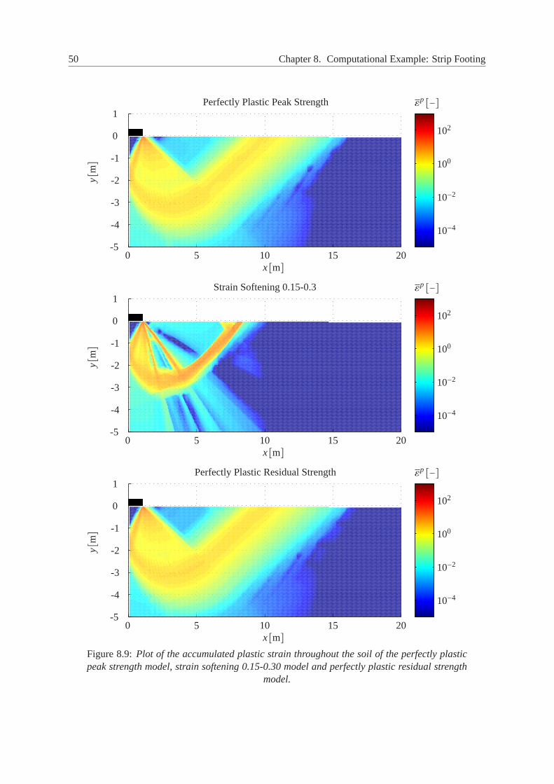
50 Chapter 8. Computational Example: Strip Footing
0
0
0
5
5
5
10
10
10
15
15
15
20
20
20
-5
-5
-5
-4
-4
-4
-3
-3
-3
-2
-2
-2
-1
-1
-1
0
0
0
1
1
1
10−4
10−4
10−4
10−2
10−2
10−2
100
100
100
102
102
102
εp[−]
εp[−]
εp[−]
x[m]
x[m]
x[m]
y[m]
y[m]
y[m]
Perfectly Plastic Peak Strength
Strain Softening 0.15-0.3
Perfectly Plastic Residual Strength
Figure 8.9:Plot of the accumulated plastic strain throughout the soil of the perfectly plasticpeak strength model, strain softening 0.15-0.30 model and perfectly plastic residual strength
model.

Chapter9
Computational Example: TunnelExcavation
To further test the approach, a tunnel excavation is carried out using an axisymmetric model, where thepurpose is to estimate the tunnel wall displacement as well as the plastic zone.
9.1 The model
The idea behind the model is to simulate a tunnel excavation in an infinite rock mass. This is done byreducing the pressure,p, on the tunnel wall, from the in situ stress state,pinf , to zero, see Figure9.1,and record the ensuing tunnel wall displacement. The radius of the tunnelis given byrT, which hasbeen set to 2,5 m. The tunnel axis is aligned in the z-direction.
Tunnel wall
Strain softening Mohr-Coulomb material
rT
p
zr
θ
Figure 9.1:Concept of the tunnel model.
The axisymmetric properties of the problem is utilized, and a 1 m section of the tunnel in thez-direction is modeled, see Figure9.2. Further, the infinite rock mass is bounded by a domain with aradius ofrBC, which has been set to 50 m in the example at hand. As with the example inchapter 8, the
51
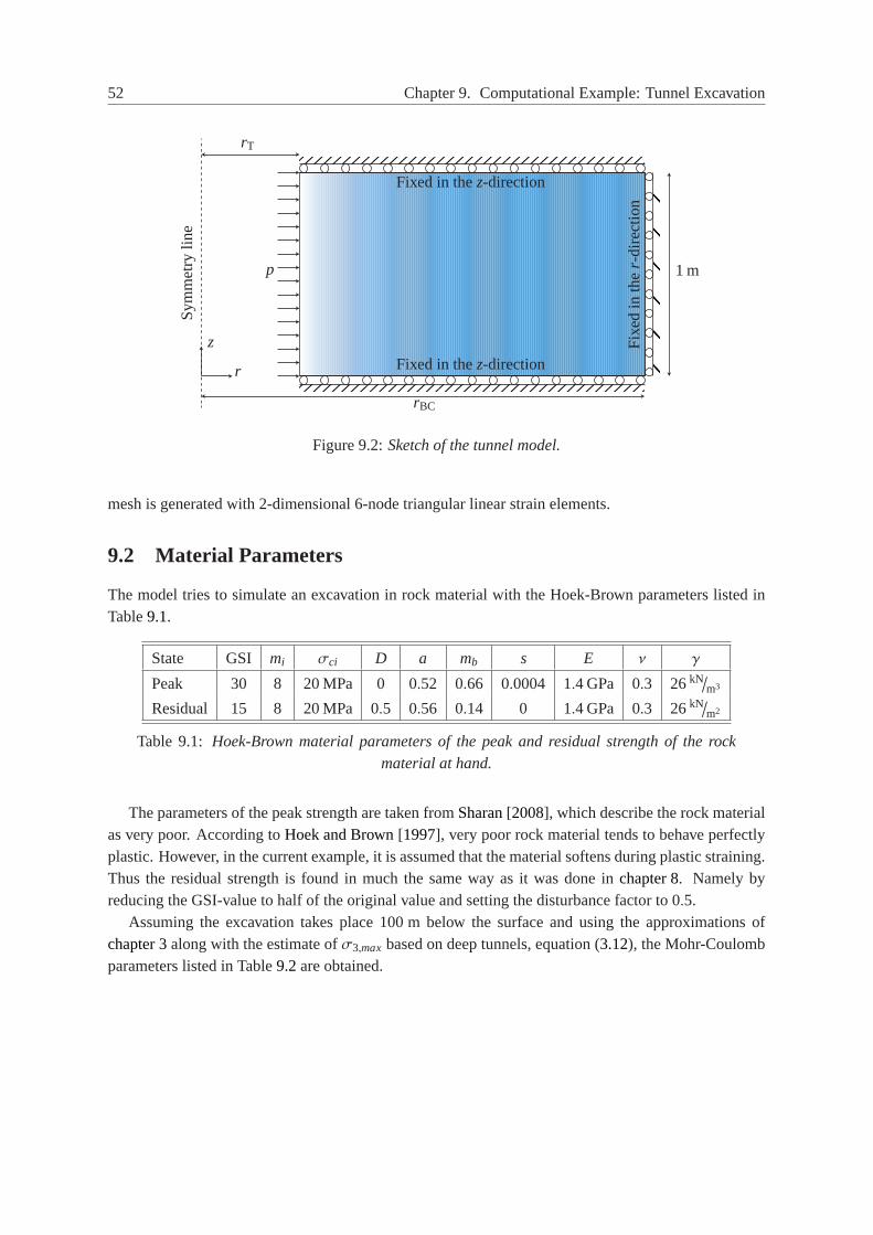
52 Chapter 9. Computational Example: Tunnel Excavation
����������������������������������������������������������������������������������������������������������������������������������������������������������������������������������������������������������������������������������������������������������������������������������������������������������������������������������������������������������������������������������������������������������������������������������������������������������������������������������������������������������������������������������������yyyyyyyyyyyyyyyyyyyyyyyyyyyyyyyyyyyyyyyyyyyyyyyyyyyyyyyyyyyyyyyyyyyyyyyyyyyyyyyyyyyyyyyyyyyyyyyyyyyyyyyyyyyyyyyyyyyyyyyyyyyyyyyyyyyyyyyyyyyyyyyyyyyyyyyyyyyyyyyyyyyyyyyyyyyyyyyyyyyyyyyyyyyyyyyyyyyyyyyyyyyyyyyyyyyyyyyyyyyyyyyyyyyyyyyyyyyyyyyyyyyyyyyyyyyyyyyyyyyyyyyyyyyyyyyyyyyyyyyyyyyyyyyyyyyyyyyyyyyyyyyyyyyyyyyyyyyyyyyyyyyyyyyyyyyyyyyyyyyyyyyyyyyyyyyyyyyyyyyyyyyyyyyyyyyyyyyyyyyyyyyyyyyyyyyyyyyyyyyyyyyyyyyyyyyyyyyyyyyyyyyyyyyyyyyyyyyyyyyyyyyyyyyyyyyyyyyyyyyyyyyyyyyyyyyyyyyyyyyyyyyyyyyyyyyyyyyyyyyyyyyyyyyyyyyyyyyyyyyy����������������������������������������������������������������������������������������������������������������������������������������������������������������������������������������������������������������������������������������������������������������������������������������������������������������������������������������������������������������������������������������������������������������������������������������������������������������������������������������������������������������������������������������yyyyyyyyyyyyyyyyyyyyyyyyyyyyyyyyyyyyyyyyyyyyyyyyyyyyyyyyyyyyyyyyyyyyyyyyyyyyyyyyyyyyyyyyyyyyyyyyyyyyyyyyyyyyyyyyyyyyyyyyyyyyyyyyyyyyyyyyyyyyyyyyyyyyyyyyyyyyyyyyyyyyyyyyyyyyyyyyyyyyyyyyyyyyyyyyyyyyyyyyyyyyyyyyyyyyyyyyyyyyyyyyyyyyyyyyyyyyyyyyyyyyyyyyyyyyyyyyyyyyyyyyyyyyyyyyyyyyyyyyyyyyyyyyyyyyyyyyyyyyyyyyyyyyyyyyyyyyyyyyyyyyyyyyyyyyyyyyyyyyyyyyyyyyyyyyyyyyyyyyyyyyyyyyyyyyyyyyyyyyyyyyyyyyyyyyyyyyyyyyyyyyyyyyyyyyyyyyyyyyyyyyyyyyyyyyyyyyyyyyyyyyyyyyyyyyyyyyyyyyyyyyyyyyyyyyyyyyyyyyyyyyyyyyyyyyyyyyyyyyyyyyyyyyyyyyyyyyyyyy������������������������������������������������������������������������������������������������������������������������������������������������������������������������������������������������
yyyyyyyyyyyyyyyyyyyyyyyyyyyyyyyyyyyyyyyyyyyyyyyyyyyyyyyyyyyyyyyyyyyyyyyyyyyyyyyyyyyyyyyyyyyyyyyyyyyyyyyyyyyyyyyyyyyyyyyyyyyyyyyyyyyyyyyyyyyyyyyyyyyyyyyyyyyyyyyyyyyyyyyyyyyyyyyyyyyyyyyyyyyyyyyyrT
rBC
Sym
met
rylin
e
1 mp
z
r
Fixed in thez-direction
Fixed in thez-direction
Fix
edin
ther
-dire
ctio
n
Figure 9.2:Sketch of the tunnel model.
mesh is generated with 2-dimensional 6-node triangular linear strain elements.
9.2 Material Parameters
The model tries to simulate an excavation in rock material with the Hoek-Brown parameters listed inTable9.1.
State GSI mi σci D a mb s E ν γ
Peak 30 8 20 MPa 0 0.52 0.66 0.0004 1.4 GPa 0.3 26kN/m3
Residual 15 8 20 MPa 0.5 0.56 0.14 0 1.4 GPa 0.3 26kN/m2
Table 9.1: Hoek-Brown material parameters of the peak and residual strength ofthe rockmaterial at hand.
The parameters of the peak strength are taken fromSharan[2008], which describe the rock materialas very poor. According toHoek and Brown[1997], very poor rock material tends to behave perfectlyplastic. However, in the current example, it is assumed that the material softens during plastic straining.Thus the residual strength is found in much the same way as it was done inchapter 8. Namely byreducing the GSI-value to half of the original value and setting the disturbance factor to 0.5.
Assuming the excavation takes place 100 m below the surface and using the approximations ofchapter 3along with the estimate ofσ3,max based on deep tunnels, equation (3.12), the Mohr-Coulombparameters listed in Table9.2are obtained.
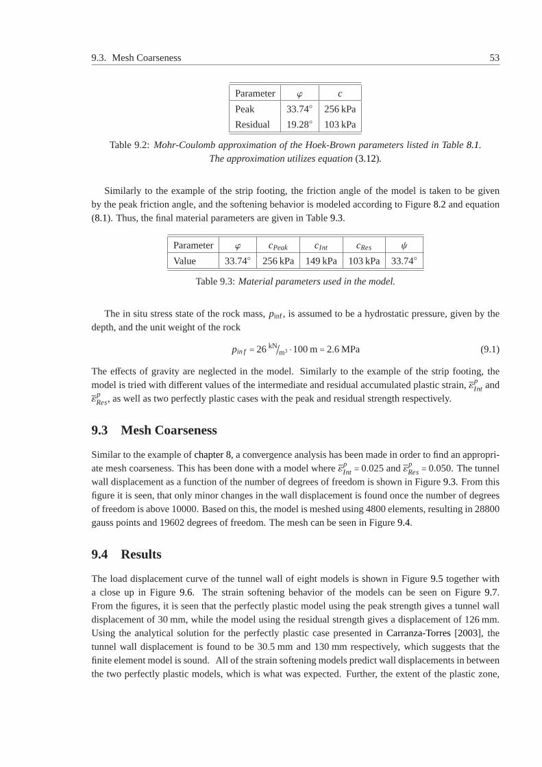
9.3. Mesh Coarseness 53
Parameter ϕ c
Peak 33.74○ 256 kPa
Residual 19.28○ 103 kPa
Table 9.2:Mohr-Coulomb approximation of the Hoek-Brown parameters listed in Table 8.1.The approximation utilizes equation(3.12).
Similarly to the example of the strip footing, the friction angle of the model is taken to be givenby the peak friction angle, and the softening behavior is modeled accordingto Figure8.2and equation(8.1). Thus, the final material parameters are given in Table9.3.
Parameter ϕ cPeak cInt cRes ψ
Value 33.74○ 256 kPa 149 kPa 103 kPa 33.74○
Table 9.3:Material parameters used in the model.
The in situ stress state of the rock mass,pinf , is assumed to be a hydrostatic pressure, given by thedepth, and the unit weight of the rock
pin f = 26kN/m3 ⋅100 m= 2.6 MPa (9.1)
The effects of gravity are neglected in the model. Similarly to the example of the strip footing, themodel is tried with different values of the intermediate and residual accumulated plastic strain,ε
pInt and
εpRes, as well as two perfectly plastic cases with the peak and residual strength respectively.
9.3 Mesh Coarseness
Similar to the example ofchapter 8, a convergence analysis has been made in order to find an appropri-ate mesh coarseness. This has been done with a model whereε
pInt = 0.025 andεp
Res= 0.050. The tunnelwall displacement as a function of the number of degrees of freedom is shown in Figure9.3. From thisfigure it is seen, that only minor changes in the wall displacement is found once the number of degreesof freedom is above 10000. Based on this, the model is meshed using 4800elements, resulting in 28800gauss points and 19602 degrees of freedom. The mesh can be seen in Figure9.4.
9.4 Results
The load displacement curve of the tunnel wall of eight models is shown in Figure 9.5 together witha close up in Figure9.6. The strain softening behavior of the models can be seen on Figure9.7.From the figures, it is seen that the perfectly plastic model using the peak strength gives a tunnel walldisplacement of 30 mm, while the model using the residual strength gives a displacement of 126 mm.Using the analytical solution for the perfectly plastic case presented inCarranza-Torres[2003], thetunnel wall displacement is found to be 30.5 mm and 130 mm respectively, which suggests that thefinite element model is sound. All of the strain softening models predict wall displacements in betweenthe two perfectly plastic models, which is what was expected. Further, the extent of the plastic zone,
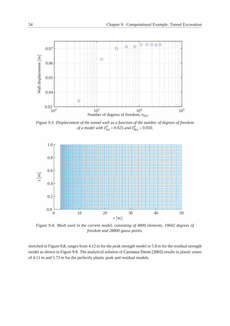
54 Chapter 9. Computational Example: Tunnel Excavation
Number of degrees of freedom,ndo f
Wal
ldis
plac
emen
t[m]
102 103 104 1050.03
0.04
0.05
0.06
0.07
Figure 9.3:Displacement of the tunnel wall as a function of the number of degrees offreedomof a model withεp
Int = 0.025andεpRes= 0.050.
r [m]
z[m]
0 10 20 30 40 500.0
0.2
0.4
0.6
0.8
1.0
Figure 9.4:Mesh used in the current model, consisting of 4800 elements, 19602 degrees offreedom and 28800 gauss points.
sketched in Figure9.8, ranges from 4.12 m for the peak strength model to 5.8 m for the residual strengthmodel as shown in Figure9.9. The analytical solution ofCarranza-Torres[2003] results in plastic zonesof 4.11 m and 5.72 m for the perfectly plastic peak and residual models.
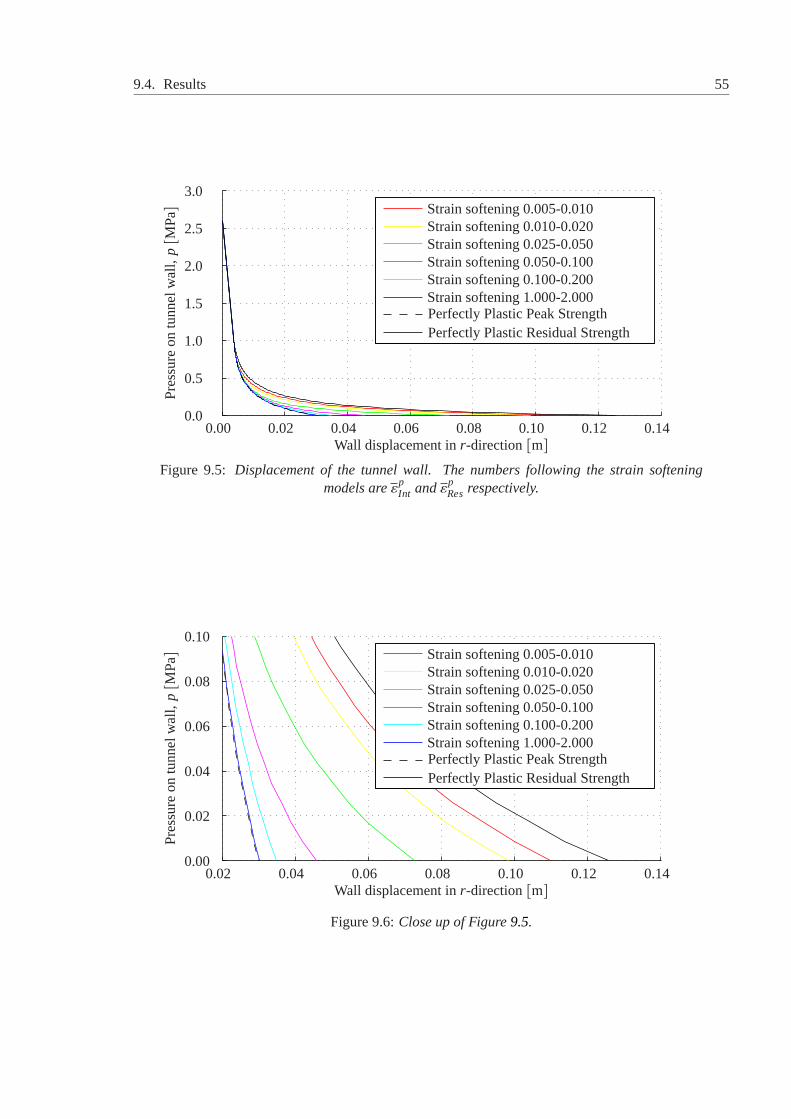
9.4. Results 55
Wall displacement inr-direction[m]
Pre
ssur
eon
tunn
elw
all,p[M
Pa]
Perfectly Plastic Peak StrengthPerfectly Plastic Residual Strength
Strain softening 0.005-0.010Strain softening 0.010-0.020Strain softening 0.025-0.050Strain softening 0.050-0.100Strain softening 0.100-0.200Strain softening 1.000-2.000
0.00 0.02 0.04 0.06 0.08 0.10 0.12 0.140.0
0.5
1.0
1.5
2.0
2.5
3.0
Figure 9.5: Displacement of the tunnel wall. The numbers following the strain softeningmodels areεp
Int andεpResrespectively.
Wall displacement inr-direction[m]
Pre
ssur
eon
tunn
elw
all,p[M
Pa]
Perfectly Plastic Peak StrengthPerfectly Plastic Residual Strength
Strain softening 0.005-0.010Strain softening 0.010-0.020Strain softening 0.025-0.050Strain softening 0.050-0.100Strain softening 0.100-0.200Strain softening 1.000-2.000
0.02 0.04 0.06 0.08 0.10 0.12 0.140.00
0.02
0.04
0.06
0.08
0.10
Figure 9.6:Close up of Figure9.5.
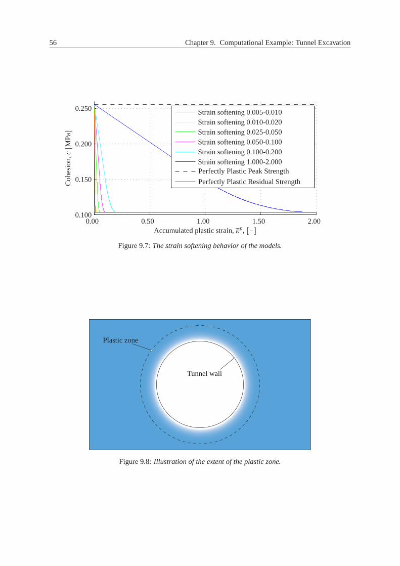
56 Chapter 9. Computational Example: Tunnel Excavation
Accumulated plastic strain,εp, [−]
Coh
esio
n,c[M
Pa]
Perfectly Plastic Peak Strength
Perfectly Plastic Residual Strength
Strain softening 0.005-0.010Strain softening 0.010-0.020Strain softening 0.025-0.050Strain softening 0.050-0.100Strain softening 0.100-0.200Strain softening 1.000-2.000
0.00 0.50 1.00 1.50 2.000.100
0.150
0.200
0.250
Figure 9.7:The strain softening behavior of the models.
Plastic zone
Tunnel wall
Figure 9.8:Illustration of the extent of the plastic zone.

9.4. Results 57
r, [m]
Acc
umul
ated
plas
ticst
rian,ε
p,[−]
Perfectly Plastic Peak StrengthPerfectly Plastic Residual Strength
Strain softening 0.005-0.010Strain softening 0.010-0.020Strain softening 0.025-0.050Strain softening 0.050-0.100Strain softening 0.100-0.200Strain softening 1.000-2.000
2.50 3.00 3.50 4.00 4.50 5.00 5.50 6.000.000
0.050
0.100
0.150
0.200
Figure 9.9:The extent of the plastic zone of the models.

Chapter10
Conclusion
The successful derivation and implementation of the strain hardening Mohr-Coulomb criterion de-scribed inchapter 7shows, that it is possible to make use of return mapping in principal stress spacefor materials, which exhibit hardening/softening properties.
The proof-of-concept examples of the strip footing and tunnel excavation show the expected results,where the strain softening materials result in solutions somewhere in between the two extremities of theperfectly plastic models using the peak and residuals strengths. Thus the hardening properties allow fora more detailed description of the problem at hand, which should result in a more safe solution, than amodel utilizing perfect plasticity along with the peak strength, as well as less conservative solution thana model utilizing perfect plasticity along with the residual strength.
Since the implemented model can handle any arbitrary development of the cohesion during plasticstraining, it should be applicable to a great deal of problems. However, as is evident from the examples,approximations to the Hoek-Brown parameters with a Mohr-Coulomb failure criterion suggest, that thefriction and dilation angles change during plastic straining as well. Something that the current model isunable to account for.
To further test the use of hardening properties along with principal stress updating schemes, a moreadvanced constitutive model, utilizing several hardening and state parameters could be developed. Forexample a Mohr-Coulomb model, where the friction and dilation angles are dependent of the stateparameters of the material. Moreover, the expressions for the consistentconstitutive matrix of two andthree active yield surfaces, equation (5.55) and (5.59), together with return mapping in principal stressspace, allows for a fairly straight forward way of developing a hardening Hoek-Brown model, whicheliminate the need for the Mohr-Coulomb approximation of hardening rock material.
Next step would be to implement these models into commercial finite element programs, in order tobe truly useful for the professional engineering community, which require ease of use and accessibility.
59

Bibliography
Carlos Carranza-Torres. Dimensionless graphical representation ofthe exact elasto-plastic solution ofa circular tunnel in a mohr-coulomb material subject to uniform far-field stresses.Rock Mechanicsand Rock Engineering, 36:237–253, 2003.
Johan Clausen.Efficient Non-Linear Finite Element Implementation of Elasto-Plasticity for Geotech-nical Problems. PhD thesis, Aalborg University, 2007.
Johan Clausen, Lars Damkilde, and Lars Andersen. Efficient return algorithms for associated plasticitywith multiple yield planes.International Journal For Numerical Methods In Engineering, 66:1036–1059, 2006.
Robert D. Cook, David S. Malkus, Michael E. Plesha, and Robert J. Witt. Concepts and Applicationsof Finite Element Analysis. John Wiley & Sons, Ltd., 2002.
Michael Anthony Crisfield.Non-Linear Finite Element Analysis. John Wiley & Sons, Ltd., 2000.
Eduardo de Souza Neto, Djordje Peric, and David Owens.Computational Methods for Plasticity -Theory and Applications. John Wiley & Sons, Ltd., 2008.
Evert Hoek.Practical Rock Engineering. 2007.
Evert Hoek and Edwin T. Brown. Practical estimates of rock mass strength. International Journal ofRock Mechanics& Mining Sciences, 34, No. 8:1165–1186, 1997.
Evert Hoek and Mark S. Diederichs. Empirical estimation of rock mass modulus. International Journalof Rock Mechanics& Mining Sciences, 43:203–215, 2006.
Evert Hoek, Carlos Carranza-Torres, and Brent Corkum. Hoek-Brown failure criterion - 2002 edition,2002.
Warner Tjardus Koiter. Stress-strain relations, uniqueness and variational theorems for elasto-plasticmaterials with a singular yield surface.Quarterly of applied mathematics., 11:350–354, 1953.
Paul Marinos and Evert Hoek. GSI: A geologically friendly tool for rock mass strength estimation.In Proceedings of the International Conference on Geotechnical and Geological Engineering, Geo-Eng2000, 2000.
61
62 Bibliography
Richard S. Merifield, Andrei V. Lyamin, and Scott W. Sloan. Limit analysis solutions for the bearingcapacity of rock masses using the generalised Hoek-Brown criterion.International Journal of RockMechanics& Mining Sciences, 43:920–937, 2006.
Joop C. Nagtegaal. On the implementation of inelastic constitutive equations with special reference tolarge deformation problems.Computer Methods in Applied Mechanics and Engineering, 33:469–484, 1982.
Niels Saabye Ottosen and Matti Ristinmaa.The Mechanics of Constitutive Modeling. Elsevier Ltd,2005.
Niels Krebs Ovesen, Leif Fuglsang, Gunnar Bagge, Anette Krogsbøll, Carsten S. Sørensen, BentHansen, Klaus Bødker, Lotte Thøgersen, Jens Galsgaard, and Anders H. Augustesen.Lærebog iGeoteknik. Polyteknisk Forlag, 2007.
Rocscience Inc. Roclab - user’s guide, 2007.
Shailendra K. Sharan. Analytical solutions for stresses and displacements around a circular opening ina generalized Hoek-Brown rock.International Journal of Rock Mechanics& Mining Sciences, 45:78–85, 2008.
Emil Smed Sørensen. Modified generalised Hoek-Brown model, 2012. Aalborg University, M.Sc. 3rdsemester report.