elasticity in microstructure sensitive design through the
TRANSCRIPT

Brigham Young University Brigham Young University
BYU ScholarsArchive BYU ScholarsArchive
Theses and Dissertations
2002-05-31
Elasticity in Microstructure Sensitive Design Through the use of Elasticity in Microstructure Sensitive Design Through the use of
Hill Bounds Hill Bounds
Benjamin L. Henrie Brigham Young University - Provo
Follow this and additional works at: https://scholarsarchive.byu.edu/etd
Part of the Mechanical Engineering Commons
BYU ScholarsArchive Citation BYU ScholarsArchive Citation Henrie, Benjamin L., "Elasticity in Microstructure Sensitive Design Through the use of Hill Bounds" (2002). Theses and Dissertations. 94. https://scholarsarchive.byu.edu/etd/94
This Thesis is brought to you for free and open access by BYU ScholarsArchive. It has been accepted for inclusion in Theses and Dissertations by an authorized administrator of BYU ScholarsArchive. For more information, please contact [email protected], [email protected].

ELASTICITY IN MICROSTRUCTURE SENSITIVE DESIGN THROUGH
THE USE OF HILL BOUNDS
by
Benjamin L. Henrie
A thesis submitted to the faculty of
Brigham Young University
in partial fulfillment of the requirements for the degree of
Master of Science
Department of Mechanical Engineering
Brigham Young University
August 2002
BRIGHAM YOUNG UNVERISTY
GRADUATE COMMITTEE APPROVAL
of a thesis submitted by
Benjamin L. Henrie
This thesis has been read by each member of the following graduate committee and by majority vote has been found to be satisfactory. ____________________________ __________________________________________ Date Brent L. Adams, Chair ____________________________ __________________________________________ Date Larry L Howell ____________________________ __________________________________________ Date Tracy W. Nelson

BRIGHAM YOUNG UNVERSITY As chair of the candidate's graduate committee, I have read the thesis of Benjamin L. Henrie in its final form and have found that (1) its format, citations, and bibliographical style are consistent and acceptable and fulfill university and department style requirements; (2) its illustrative materials including figures, tables, and charts are in place; and (3) the final manuscript is satisfactory to the graduate committee and is ready for submission to the university library. ____________________________ __________________________________________ Date Brent L. Adams, Chair Accepted for the Department __________________________________________ Larry L Howell Department Chair Accepted for the College __________________________________________ Douglas M Chabries Dean, College of Engineering and Technology
ABSTRACT
ELASTICITY IN MICROSTRUCTURE SENSITIVE DESIGN THROUGH
THE USE OF HILL BOUNDS
Benjamin L. Henrie
Department of Mechanical Engineering
Master of Science
In engineering, materials are often assumed to be homogeneous and isotropic; in
actuality, material properties do change with sample direction and location. This variation
is due to the anisotropy of the individual grains and their spatial distribution in the
material. Currently there is a lack of communication between the design engineer,
material scientist, and processor for solving multi-objective/constrained designs. If
communication existed between these groups then materials could be designed for
applications, instead of the reverse. Microstructure sensitive design introduces a common
language, a spectral representation, where both design properties and microstructures are
expressed.
Using Hill bounds, effective elastic properties are expressed within the spectral
representation. For the elastic properties, two FCC materials, copper and nickel, were
chosen for computation and to demonstrate how symmetry enters into the methodology.
This spectral representation renders properties as hyper-surfaces that translate through a
multi-dimensional Fourier space depending on the property value of the hyper-surface.
Property closures are generated by condensing the information contained within the
multi-dimensional Fourier space into a 2-D representation. This compaction of
information is beneficial for a quick determination of property limits for a particular alloy
system. The design engineer can now dictate the critical design properties and receive
sets of microstructures that satisfy the design objectives.

ACKNOWLEDGMENTS
This research was supported by funding from the army research office (ARO).
This assistance is gratefully acknowledged.
I would like to thank Dr. Brent L. Adams for the many hours he has spent going
over theory and encouragement. I want to especially thank him for the opportunity to
work with him and his research team. He has greatly influenced my path through
schooling, and through out my life.
I also want to thank my graduate committee, Dr. Nelson and Dr. Howell.
I would like to thank my parents for helping me to have the dream to pursue my
education and their financial help in the beginning. They have been a source of
encouragement even when they thought that I would never finish.
My wife has been wonderful through the entire experience. Alisa has forever
changed the way my life is headed: First by marrying me and then by redirecting my
degree from Electrical Engineering to Mechanical Engineering. She is responsible for
starting my undergraduate research with Dr. Adams and encouraging me when life was
hard. She is the best thing that has ever happened to me.

Table of Contents
List of Figures .................................................................................................................... ix
List of Tables ..................................................................................................................... xi
1 Introduction................................................................................................................. 1
1.1 Overview......................................................................................................... 1
1.2 History of Microstructure Sensitive Design ................................................... 2
1.3 Elasticity ......................................................................................................... 4
2 Local State Space........................................................................................................ 7
2.1 Overview......................................................................................................... 7
2.2 Local States..................................................................................................... 7
2.3 Local State Space............................................................................................ 8
2.4 Basis Functions ............................................................................................... 9
2.5 Fourier Representation of the Local State Space.......................................... 10
2.6 Microstructure Hull....................................................................................... 11
3 Elasticity, Hill Bounds .............................................................................................. 13
3.1 Overview....................................................................................................... 13
3.2 Elastic Homogenization Relations................................................................ 13
3.3 Fourier Representation of the Upper Bound................................................. 15
3.4 Fourier Representation of the Lower Bound ................................................ 18
3.4.1 Inversion of the Lower Bound .......................................................... 20
4 Alloy System............................................................................................................. 23
4.1 Overview....................................................................................................... 23
4.2 Elastic Bounds with Crystal and Sample Symmetry .................................... 23
5 Elastic Properties in Fourier Space ........................................................................... 29
5.1 Overview....................................................................................................... 29
5.2 Hyper-Surfaces in the Fourier Space ............................................................ 29
vii
5.3 Extraction of Microstructures from the Fourier Space ................................. 33
6 Property Closures...................................................................................................... 35
6.1 Overview....................................................................................................... 35
6.2 Generation of the Property Closures............................................................. 35
6.3 Benefits of the Property Closures ................................................................. 36
7 Conclusions and Recommendations ......................................................................... 39
7.1 Conclusions................................................................................................... 39
7.2 Recommendations......................................................................................... 40
References......................................................................................................................... 41
Appendix........................................................................................................................... 45
Appendix A : Property Closures ............................................................................... 45
Appendix B : Inversion for cubic-orthorhombic symmetry ..................................... 52
Appendix C :Program for generation of the property closures................................. 54
Appendix D : Program for generation of the upper-bound....................................... 57
Appendix E : Program for generation of the lower-bound ....................................... 59
Appendix F : Program for computing the ηφ 1*lrD coefficients................................... 63
Appendix G : Harmonics.h subroutine ..................................................................... 65
Appendix H : Property.h subroutine ......................................................................... 76
viii
List of Figures
Figure 1.1 Ashby chart of youngs modulus vs. strength (Ashby, 1992) ............................ 2
Figure 1.2 MSD paradigm –new approach ......................................................................... 4
Figure 2.1 Piecewise constant function ............................................................................ 10
Figure 2.2 Cubic-orthorhombic microstructure hull ......................................................... 12
Figure 3.1 Elastic constants of Cu-Ni alloys for values predicted by Hartley and those
obtained from experiments. Hartley (2001).............................................................. 17
Figure 4.1 Copper-Nickel alloy system ............................................................................ 24
Figure 4.2 Number of linearly independent spherical harmonics of different symmetries
as a function of degree l (for even l). (Bunge1982).................................................. 26
Figure 4.3 Number of linearly independent spherical harmonics of different symmetries
as a function of degree l (for odd l). (Bunge 1982) .................................................. 26
Figure 5.1 Elastic upper-bound of >< 1111C and >< 1212C in the microstructure hull.... 30
Figure 5.2 Elastic lower-bound of the hyper-surface < 11111−>S in the microstructure hull
................................................................................................................................... 32
Figure 5.3 Microstructure hull with < 11111−>S and >< 1212C hyper-surfaces. The area in
yellow contains those microstructures that fulfill the design constraints. ................ 33
Figure 5.4 One extracted microstructure that satisfy both the < 11111−>S and
>< 1212C bounds........................................................................................................ 34
Figure 6.1 Property closure of C *1111 vs. *
1212C of the Cu-Ni alloy system........................ 37
Figure 6.2 Property closure of C *1111 vs. *
1212C with design constraints added at A and B 37
Figure A.1 Property closure of C vs. ................................................................. 45 *1111
*2222C
Figure A.2 Property closure of C vs. ................................................................. 45 *1111
*3333C
Figure A.3 Property closure of C vs. ................................................................. 46 *1111
*2323C
ix
Figure A.4 Property closure of C vs. ................................................................. 46 *1111
*3131C
Figure A.5 Property closure of C vs. ................................................................ 47 *2222
*3333C
Figure A.6 Property closure of C vs. ................................................................ 47 *2222
*2323C
Figure A.7 Property closure of C vs. ................................................................. 48 *2222
*3131C
Figure A.8 Property closure of C vs. ................................................................. 48 *2222
*1212C
Figure A.9 Property closure of C vs. ................................................................. 49 *3333
*2323C
Figure A.10 Property closure of C vs. ............................................................... 49 *3333
*3131C
Figure A.11 Property closure of C vs. ............................................................... 50 *3333
*1212C
Figure A.12 Property closure of C vs. ............................................................... 50 *2323
*3131C
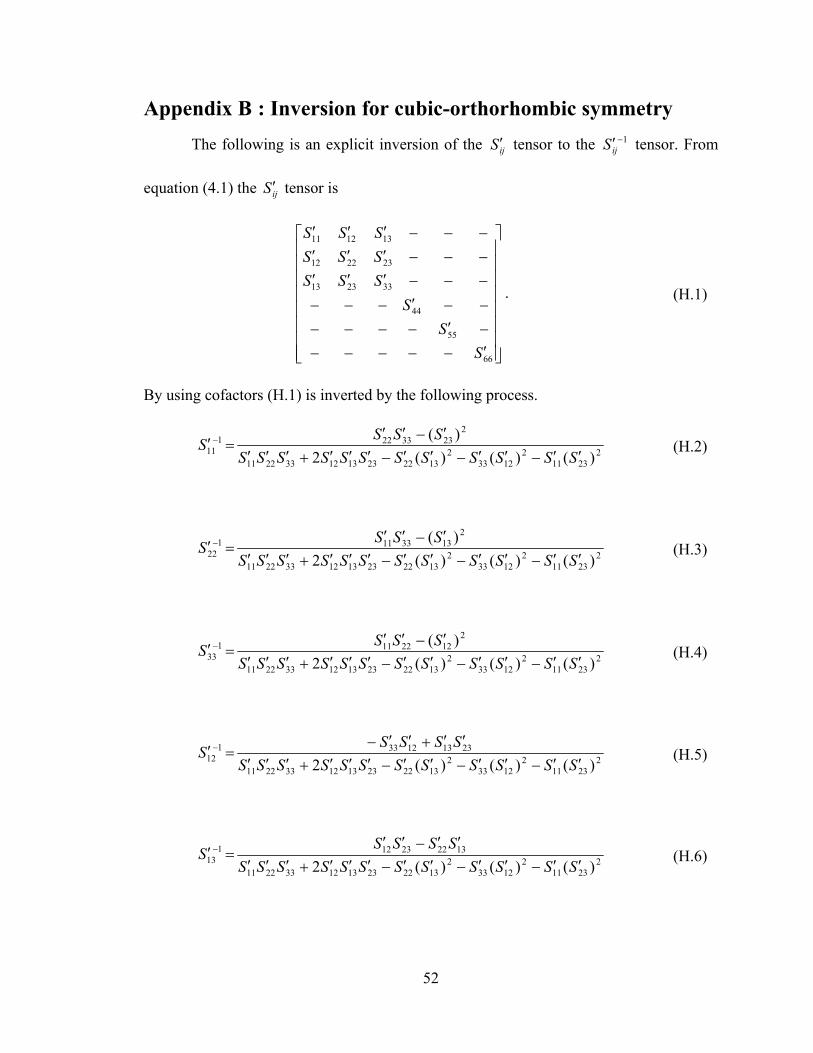
Figure A.13 Property closure of C vs. ............................................................... 51 *2323
*1212C
Figure A.14 Property closure of C vs. ............................................................... 51 *3131
*1212C
x

List of Tables
Table 3.1 Transforming from four indices, ijkmS , to two indices, ijS ............................... 21
Table 5.1 µ1
lD coefficients for the cubic-orthorhombic case for the on-diagonal elements
................................................................................................................................... 31
xi

xii

1 Introduction
1.1 Overview
In engineering, materials are assumed to be homogeneous and isotropic; in
actuality, material properties do change with sample direction and location. This variation
is due to the anisotropy of the individual grains and their spatial distribution in the
material. This thesis will develop the basic methodology of Microstructure Sensitive
Design, through the use of elastic bounds (Hill bounds), and demonstrate how
microstructures can be used as a design parameter.
Charts, such as Ashby charts ( Figure 1.1, Ashby, 1992), have been compiled to
show property limits of the generic materials database, but these charts do not take into
account the microstructure of the material. If microstructure and composition are taken
into account, more property variance is predicted.
With highly constrained design, e.g. space shuttle, the design engineer may
discover that there are no materials that will satisfy the design objectives. Typically
design materials are selected first for design work, but if the material is a design variable
than great design freedom can be achieved.
The traditional approach for material insertion is Material Scientist Processor
Design Engineering. Scientists and Processing Engineers try to develop materials
with improved properties to impart to the Design Engineers. If the new material has
→
→
1
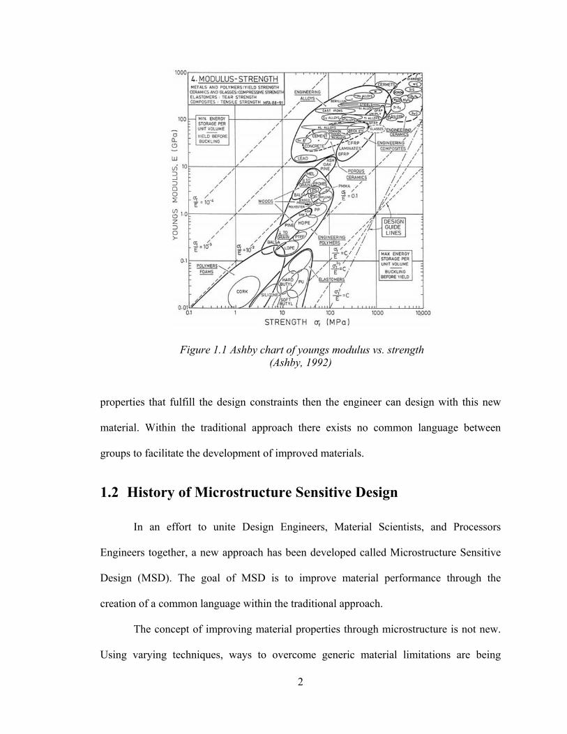
Figure 1.1 Ashby chart of youngs modulus vs. strength (Ashby, 1992)
properties that fulfill the design constraints then the engineer can design with this new
material. Within the traditional approach there exists no common language between
groups to facilitate the development of improved materials.
1.2 History of Microstructure Sensitive Design
In an effort to unite Design Engineers, Material Scientists, and Processors
Engineers together, a new approach has been developed called Microstructure Sensitive
Design (MSD). The goal of MSD is to improve material performance through the
creation of a common language within the traditional approach.
The concept of improving material properties through microstructure is not new.
Using varying techniques, ways to overcome generic material limitations are being
2
developed. Larsen (et al., 1997) used topology optimization to find microstructures that
exhibit negative poison’s ratios for compliant micro-mechanisms. Design of
piezocomposities by the same method was performed by Sigmund (et al., 1998). Olhoff
(et al., 1998) extended these methods to consider three-dimensional elastic continuum
structures. Olsen (1998) and Subbarayan and Raj (1999) have proposed methods of
integrating material science with engineering to improve the development of new
materials.
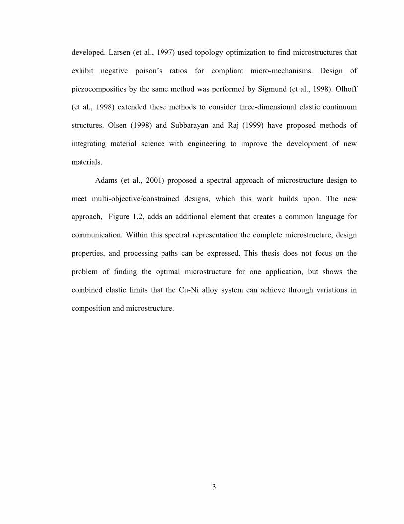
Adams (et al., 2001) proposed a spectral approach of microstructure design to
meet multi-objective/constrained designs, which this work builds upon. The new
approach, Figure 1.2, adds an additional element that creates a common language for
communication. Within this spectral representation the complete microstructure, design
properties, and processing paths can be expressed. This thesis does not focus on the
problem of finding the optimal microstructure for one application, but shows the
combined elastic limits that the Cu-Ni alloy system can achieve through variations in
composition and microstructure.
3

Figure 1.2 MSD paradigm –new approach
1.3 Elasticity
One material property of importance to many designs is elasticity. For example
beam deflection, as required in compliant mechanisms (Howell, 2001), depends on this
material property. The prediction of elastic properties has been a recurring undertaking in
the literature. Voigt (1928) proposed to estimate the elastic moduli by the assumption that
strain is uniform throughout an aggregate. Reuss (1929) proposed to estimate the elastic
moduli using the assumption that stress is uniform throughout an aggregate. Hill (1952)
demonstrated that the Voigt and Reuss averages had produced upper and lower bounds to
the measured elastic moduli. Hashin and Shtrikman (1962a, 1962b), using a variation
principle, developed narrower bounds than those obtained by the Voigt and Reuss
averages. Beran (et al., 1996) adapted the Hashin and Shtrikman variational principle to
obtain improved bounds for the effective stiffness tensor in orthotropic materials.
4

In the present work the Hill bounds are used to produce combined elastic
properties closures for the Cu-Ni system covering the complete range of composition and
microstructure. These closures permit an engineer to identity if the Cu-Ni system satisfies
the required elasticity for a design. Additionally the Hill bounds are expressed as a
Fourier series for use in the spectral representation.
5

6

2 Local State Space
2.1 Overview
Before properties can be expressed within the common language, the spectral
representation must be defined. The local states space is defined on the premise that
salient local properties are dependent upon a small number of local state variables. The
local state space is a collection of all possible local states. This state space is later
translated into a set of Dirac functions in the Fourier space. Weighted combinations of
these Dirac functions will be used to represent all possible microstructures on the local
state space. Representation of the local state space and the set of all possible
microstructures in their Fourier components constitutes the spectral representation.
2.2 Local States
The basic premise behind MSD is that salient local properties, pi, are dependent
upon a small number of local state variables, h, that are presumed known to the observer,
)(hpp ii = . (2.1)
Local states can be crystal orientation, composition, reference shear stress for dislocation
slip, and others. Through homogenization relationships the local properties, and their
distribution in the microstructure, are linked with estimated effective (macroscopic)
properties (Chapter 3).
7
In this work three local state variables are employed
),,( λφ gh = , (2.2)
where φ is phase, g is lattice orientation, and λ is composition. These local state
variables belong to the sets Φ=∈ }...,3,2,1{ nφ , , and Γ= φφGSOg /)3(∈ Λ=∈ ]1,0[λ .
is the 3-dimensional special orthogonal group of rotations of the crystal lattice,
and is the crystallographic symmetry subgroup of phase
)3(SO
Gφ φ . Thus, φΓ represents the
set of all physically distinctive orientations of the crystal lattice associated with phase φ
(Adams and Olson 1998). λ represents composition for this work, but λ can be utilized
for any scalar parameter.
2.3 Local State Space
The local state space, H, shall consist of all possible (ordered) sets of local state
variables. Local state is defined as one element of the local state space. If only a single
phase material is considered then
Λ×Γ=∈ φHh . (2.3)
If the material is a two phase system then
)( 21 HHHh ∪=∈ . (2.4)
where 1H and 2H are defined by
Λ×Γ= φφH . (2.5)
8
2.4 Basis Functions
Following Bunge (1982), the classical crystal symmetric generalized spherical
harmonic functions, , are used to represent the orientation dependence on )(gT mnl Γφ .
The crystal symmetric basis functions, , are special linear combinations of the
generalized spherical harmonic functions,
)(gTlµυφ &&&
∑ ∑+
−=
+
−=
=l
lm
l
ln
mnl
nl
mll gTAAgT )()( υφµφµυφ &&&&&& .
(2.6)
The symmetry coefficients, , carry the crystal symmetry and the coefficients, ,
carry the sample symmetry. The functions form a complete system of
orthonormal functions with the following property:
µφ mlA&& υφ n
lA&
)(gT mnl
∫Γ
′′′+=
φ
δδδ nnmmllmn
lmn
l ldggTgT
121)()( * ,
(2.7)
where * is the complex conjugate.
Piecewise constant functions are used to provide the basis for composition
dependence on . Λ )(λχ r are defined to be piecewise constant functions (Keener, 2000)
defined on subintervals of the range of rλ (as enumerated by the index r), as shown in
Figure 2.1. Thus,
∈
=otherwise
ifM rrr 0
)(/1)(
λλλλχ .
(2.8)
These form a complete system of orthonormal functions
∫ ′′ =
r r
rrrr M
dλ λ
δλλχλχ
)()()( ,
(2.9)
9
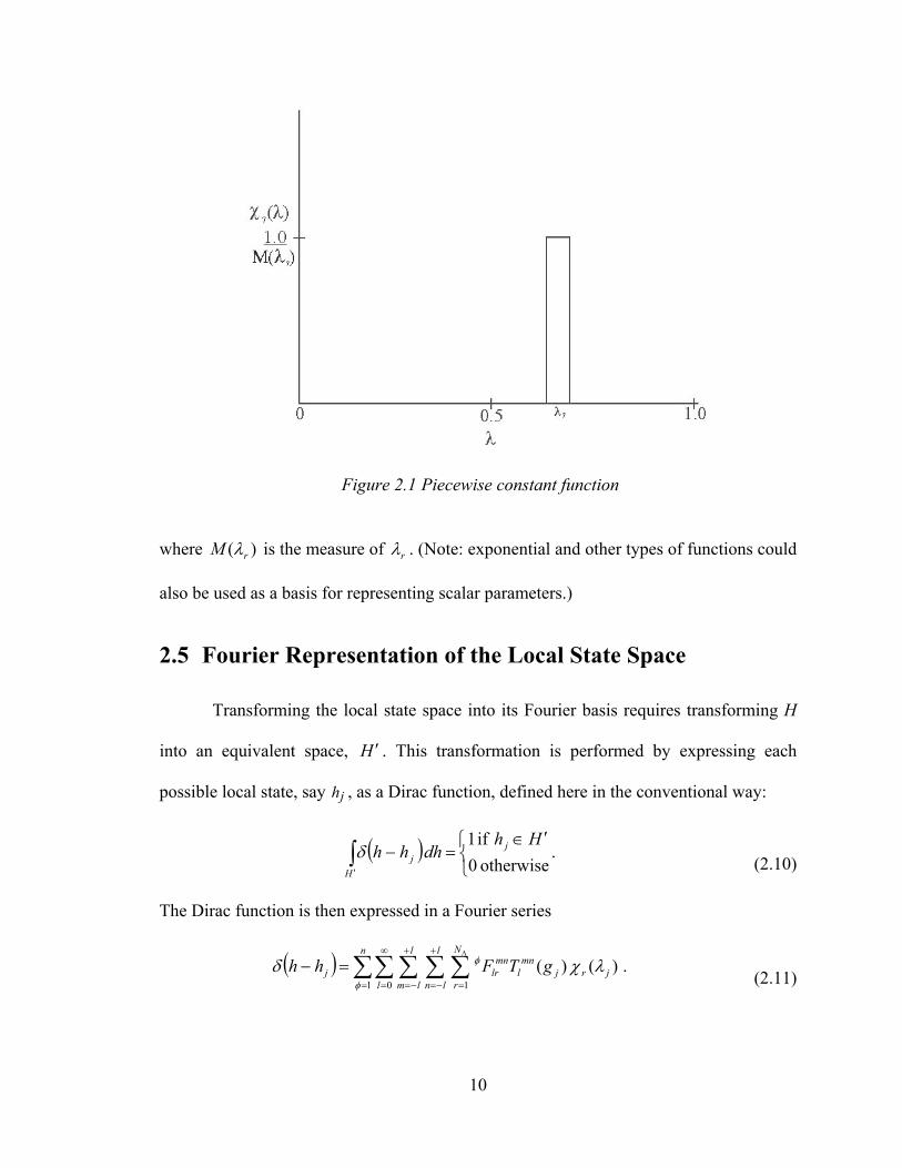
Figure 2.1 Piecewise constant function
where )( rM λ is the measure of rλ . (Note: exponential and other types of functions could
also be used as a basis for representing scalar parameters.)
2.5 Fourier Representation of the Local State Space
Transforming the local state space into its Fourier basis requires transforming H
into an equivalent space, H ′ . This transformation is performed by expressing each
possible local state, say h , as a Dirac function, defined here in the conventional way: j
( ) ′∈
=−∫′ otherwise 0
if 1 Hhdhhh j
Hjδ .
(2.10)
The Dirac function is then expressed in a Fourier series
( ) ∑∑ ∑ ∑ ∑=
∞
=
+
−=
+
−= =
Λ
=−n
l
l
lm
l
lnjrj
N
r
mnl
mnlrj gTFhh
1 0 1)()(
φ
φ λχδ . (2.11)
10
From relations (2.7) and (2.9), the Fourier coefficients of the Dirac function have the
form
)()()()12( *jrj
mnlj
mnlr gTMlF λχλφ += .
(2.12)
2.6 Microstructure Hull
For the homogenization relations of interest in Chapter 3, microstructure is
specified by the local state distribution function, , which defines the volume fraction
of sample volume that lies within a range dh of local state h:
)(hf
VdV /
dhhfVdV )(= . (2.13)
(2.13)
Here dh is the invariant measure (see Bunge, 1982). The local state distribution function,
, is normalized ,as can be seen from equation , according to )(hf
∫ = 1)( dhhf (2.14)
and expressed as a series of generalized spherical harmonics functions (Courant and
Hilbert, 1989),
)()()(0 1 1
λχφr
l
l
n
l
lm
N
r
mnl
mnlr gTFhf ∑∑∑∑
∞
=
+
−=
+
−= =
Λ
= . (2.15)
It is convenient to represent as a summation of Dirac functions, weighted by the
appropriate volume fractions,
)(hf
jν ,
∑=
−=N
jjj hhhf
1)()( δν .
(2.16)
The set of volume fractions, jν , are constrained to sum to one:
11
∑ =j
j 1ν . (2.17)
This local state distribution resides in an infinite-dimensional Fourier space, although the
homogenization relations introduced in Chapter 3 require only finite-dimensional
approximations of . )(hf
The set of all possible is called the microstructure hull; it consists of all
possible microstructures pertinent to the chosen homogenization relations and local state
space. Formally, the microstructure hull, as described in the Fourier space, obtained from
relations (2.11, 12, and 14) when constrained by (2.15) (see Adams et al. 2001).
Graphically, this microstructure hull is difficult to view because of the infinite-
dimensional nature of the Fourier space in which it resides; however for the
homogenization relations (Hill bounds) of interest in this thesis (Chapter 3), with cubic-
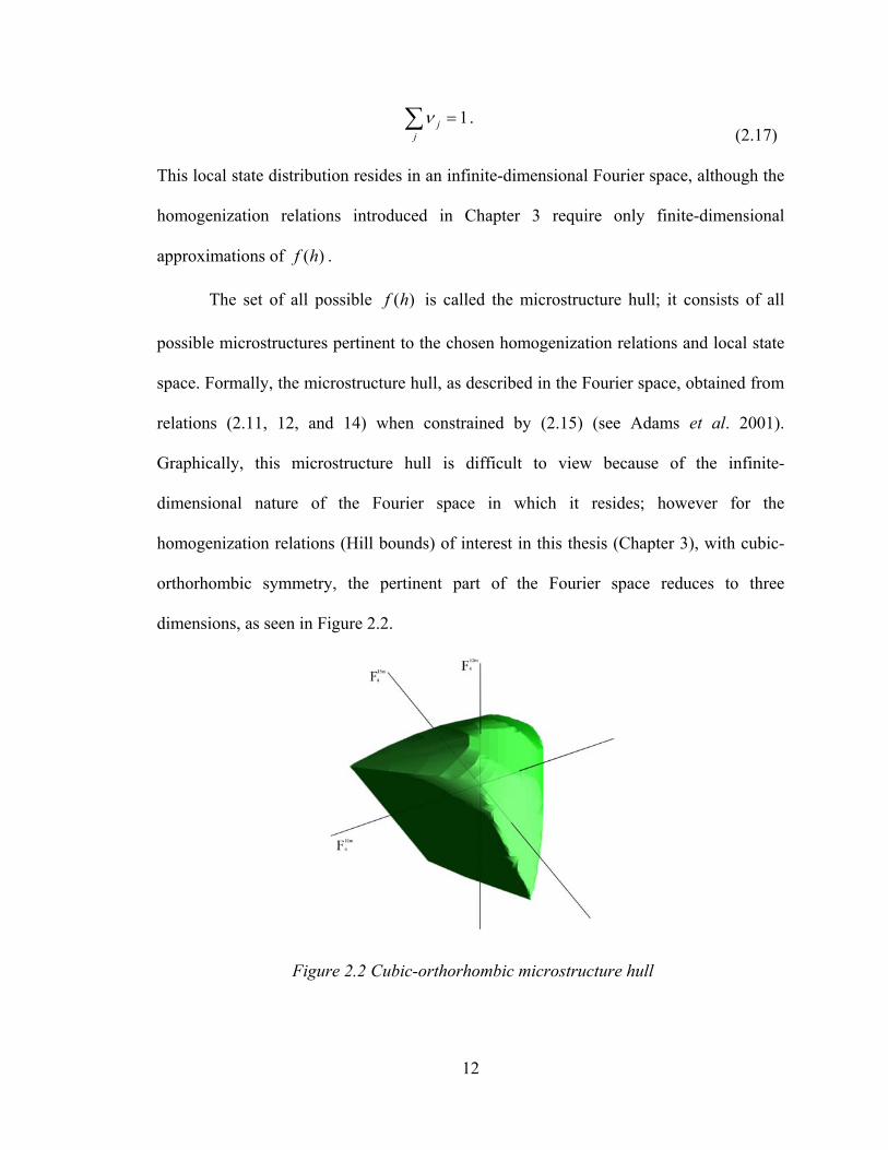
orthorhombic symmetry, the pertinent part of the Fourier space reduces to three
dimensions, as seen in Figure 2.2.
)(hf
Figure 2.2 Cubic-orthorhombic microstructure hull
12

3 Elasticity, Hill Bounds
3.1 Overview
The design engineer's input into MSD is to specify the significant effective
properties. By specifying the local properties, the designer makes certain that
microstructures are chosen that fulfill the design objectives. Through the use of elastic
homogenization relationships the effective elastic properties are linked with the local
elastic properties, and their distribution in the microstructure. Using work performed by
Hill (1952) the effective elastic properties are estimated through upper and lower bounds.
These bounds are then represented by a series of basis functions described in section 2.4.
For this chapter, consideration of symmetry is omitted to simplify the general overview
of the theoretical development.
3.2 Elastic Homogenization Relations
The stiffness tensor, Cijkm1, relates stress to strain by Hooke’s law
kmijkmij C εσ = . (3.1)
Here σij is the stress tensor, and εkm is the strain tensor. The compliance tensor, Sijkm, is
derived from the stiffness tensor by
1 Repeated indices implies summation over the integers 1,2,3 according to the Einstein summation convention, except as otherwise noted.
13

][21
jpiqjqipkmpqijkm SC δδδδ += (3.2)
where δip is the Kronecker Delta2. Compliance is defined by the relation
kmijkmij S σε = . (3.3)
Hill (1952) demonstrated that the Voigt and Reuss averages were really upper and
lower elastic bounds. Following Hill, we define the effective stiffness, C , as *ijkm
kmij ijkmC εσ *= ,
(3.4)
where < > denotes volume average quantities. The effective tensor is determined from
knowledge of the single crystal tensor and the statistical properties of the microstructure.
Compliance has a similar effective tensor.
Beran (1996) showed that the upper and lower bounds of the effective tensor can
be calculated through two classical variational principles: the principle of minimum
potential energy, and the principle of complementary energy. These principles for the
effective stiffness tensor form lower and upper bounds
kmijkmijkmijkmijkmijkmij CCS εεεεεε ≤≤− *1 . (3.5)
A similar expression for can be derived. *ijkmS
Evaluation of (3.5) does not directly provide bounds for all components of C .
Direct bounds obtained only for (no sum on i) and C (no sum on i or j,
*ijkm
*iiiiC *
ijij ji ≠ ).
Bounds can be found for off diagonal elements, but some additional work is required.
This thesis will focus on bounds for the “on-diagonal” cases.
2 The Kronecker Delta function is expressed as
≠=
=)(0)(1
piifpiif
δ
14
3.3 Fourier Representation of the Upper Bound
Equation (3.5) for the upper bound can be expressed in terms of the local state
density function as
∑ ∫∫∫ ∫= Λ
=n
GSOijkmijkm dgdgCgfC
1 /)3(
),(),,(φ
φ λλλφφ
(3.6)
where dg is the invariant measure in orientation space, 21)sin( ϕθϕθ ddd , and 21 ,, ϕθϕ
are the Euler angles defined by Bunge(1982). Both ),,( λφ g (φCijkmf and are real-
valued functions on the local state space, H.
),λg
Since is the elastic stiffness tensor in the sample coordinate frame a
relationship must be found to relate with the elastic stiffness tensor in the
crystal coordinate frame, . This relationship is required because the elastic
constants, i.e. (Hirth and Lothe 1968), are measured in the
crystal coordinate frame. is
),( λφ gCijkm
),(11 λ φφ oC
),( λφ gCijkm
)(λ
)(λφ oijkmC
),( 4412 λ φ oo C
)(λoijkmC
C
φ
])[()()( 4412 jkimjmikkmijijkm CCC δδδδλδδλλ φφφ ++= ooo . (3.7)
Using the “passive” notation3, as used by Bunge (1982), the direction cosines, gij,
are defined as
ojiji ege = .
(3.8)
The rotation from the crystal frame to the sample frame is performed as
3 The passive notation is of the form )()( gfggf =oφ
φg where g transforms a sample fixed coordinate
system, Ka into a crystal fixed coordinate system Kb. is a rotation that transforms a crystal from one orientation to a symmetrically equivalent orientation.
15

)(),( λλ φφ oijkmdmckbjaiabcd CgggggC = .
(3.9)
For cubic symmetry (3.9) can be written in a simpler form as
rmrkrjri
jkimjmikkmijijkm
ggggCCC
CCgC
)](2)()([
])[()(),(
441211
4412
λλλ
δδδδλδδλλφφφ
φφφ
ooo
oo
−−
+++=.
(3.10)
The relationship implies a summation over r from 1 to 3: rmrkrjri gggg
mkjimkjimkjirmrkrjri gggggggggggggggg 333322221111 ++= (3.11)
Hartley (2001) describes a method for finding the material constants, , for a
homogenous composition of two materials. Figure 3.1 shows Hartley's predictions for the
material constants of the Cu-Ni alloy system, and their comparison to measured values.
)(λφ oijC
Relation (3.10) is divided into two parts
])[()( 4412 jkimjmikkmijijkm CCA δδδδλδδλ φφφ ++= oo (3.12)
and
rmrkrjriijkm ggggZ )(λβφφ = (3.13)
for a more simple transformation with basis functions. is given as )(λβφ
∑Λ
=
=−−=N
rrrCCC
1441211 )()(2)()()( λχβλλλλβ φφφφφ ooo . (3.14)
Also, (3.12) is expressed using piecewise functions,
∑Λ
=
=N
rrrijkm ijkmkA
1
)()( λχφφ , (3.15)
and (3.13) as a combination of piecewise and generalized spherical harmonic functions,
∑ ∑ ∑∑=
+
−=
+
−= =
Λ
=4
0 1
** )()()(l
l
lm
l
ln
N
rr
mnl
mnlrijkm gTijkmDZ λχβ φφφ . (3.16)
16

Figure 3.1 Elastic constants of Cu-Ni alloys for values predicted by Hartley and those obtained from experiments. Hartley (2001)
The two coefficients and maybe expressed as one coefficient, but the
coefficients do not change with composition. From this property the
coefficients are only calculated once for a set symmetry. The
coefficients change for each alloy system, and require much less computational time.
rβφ )(* ijkmD mn
lφ
)(* ijkmD mnl
φ
)(* ijkmD mnl
φrβ
φ
Equation (3.16) shows that l needs to be enumerated only up to 4, due to the fact
that it is the product of four direction cosines (Bunge, 1982):
∑ ∑ ∑=′
+
−=′
+
−=′
′′′
′′′=
4
0
** )()(l
l
lm
l
ln
nml
nmlrmrkrjri gTijkmDgggg φ .
(3.17)
Combining (3.15) and (3.16), becomes ijkmCφ
17

∑ ∑∑∑∑Λ Λ
= =
+
−=
+
−= =
+=N
r l
l
lm
l
ln
N
rr
mnl
mnlrrrijkm gTijkmDijkmkC
1
4
0 1
** )()()()()( λχβλχ φφφφ . (3.18)
By combining equations (2.15), (3.6), and (3.18) the stiffness upper bound
becomes
mnlr
mnlrl
n
l
l
lm
l
ln
N
rrijkmijkm FijkmDijkmkCC φφφ
φ
φ βδ )]()([ *0
1
4
0 1
* +=≤ ∑∑∑∑∑= =
+
−=
+
−= =
Λ
. (3.19)
From (3.19) the upper bound can be calculated for all pertinent microstructures and
compositions. Note that the upper-bound relationship in (3.18) comprises, for fixed
, a hyper-plane within the Fourier space. This hyper-plane consists of all Fourier
components
Cijkm*
φFlrmn , representing microstructures, which possess the same upper bound on
effective stiffness.
3.4 Fourier Representation of the Lower Bound
The procedure for finding the elastic property closures for the lower bound is
similar to the upper bound approach except for an inversion. From equation (3.5) the
lower bound is
1−
ijkmS .
(3.20)
Before the inversion can be performed the average compliance tensor is computed from
the local state distribution function:
∑ ∫∫∫ ∫= Λ
=n
GSOijkmijkm dgdSgfS
1 /)3(
)(),,(φ
φ λλλφφ
. (3.21)
Relation (3.9) is changed to
)(),( λλ φφ oijkmdmckbjaiabcd SgggggS = ,
(3.22)
18

where is oijkmSφ
))(()()( 4412 jkimjmikkmijijkm SSS δδδδλδδλλ φφφ ++= ooo . (3.23)
Equation (3.22) can be expressed in a simpler form for cubic symmetry as
rmrkrjri
jkimjmikkmijijkm
ggggSSS
SSgS
)](2)()([
])[()(),(
441211
4412
λλλ
δδδδλδδλλφφφ
φφφ
ooo
oo
−−
+++=.
(3.24)
Hartley's method is again utilized (see section 3.3) for a homogenous composition of two
materials. Equation (3.24) is broken up into two parts
])[()( 4412 jkimjmikkmijijkm SSE δδδδλδδλ φφφ ++= oo (3.25)
and
rmrkrjriijkm ggggQ )(λαφφ = , (3.26)
where is αφ
∑Λ
=
=−−=N
rrrSSS
1441211 )()(2)()()( λχαλλλλα φφφφφφ ooo . (3.27)
(3.25) is expressed with piecewise constant functions,
∑Λ
=
=N
rrrijkm ijkmkE
1)()( λχφφ , (3.28)
and (3.26) is a combination of piecewise and harmonic functions,
∑∑ ∑∑=
+
−=
+
−= =
Λ
=4
0 1
** )()()(l
l
lm
l
ln
N
rr
mnl
mnlrijkm gTijkmDQ λχα φφφ . (3.29)
Combining (3.28) and (3.29), becomes ijkmSφ
∑ ∑ ∑∑∑=
+
−=
+
−= ==
ΛΛ
+=4
0 1
**
1)()()()()(
l
l
lm
l
ln
N
rr
mnl
mnlr
N
rrrijkm gTijkmDijkmkS λχαλχ φφφφ . (3.30)
19

The stiffness lower bound, before inversion, is found by joining equations (2.15), (3.21),
and (3.30),
mnlr
mnlrl
n
l
l
lm
l
ln
N
rrijkm FijkmDijkmkS φφφ
φ
φ αδ )]()([ *0
1
4
0 1+=∑ ∑∑ ∑∑
= =
+
−=
+
−= =
Λ
. (3.31)
3.4.1 Inversion of the Lower Bound
By setting jiij σσ = and jiij εε = the fourth rank tensor reduces from 81 terms to
36 terms, which can be written in matrix form as
(3.32)
(3.32)
=
12
31
23
12
31
23
33
22
11
121231122312
311231312331
231223312323
121231122312
311231312331
231223312323
331222121112
333122311131
332322231123
121231122312
311231312331
231223312323
121231122312
311231312331
231223312323
331222121112
333122311131
332322231123
331233313323
221222312223
111211311123
331233313323
221222312223
111211311123
333322331133
223322221122
113311221111
12
31
23
12
31
23
33
22
11
σσσσσσσσσ
εεεεεεεεε
SSSSSSSSS
SSSSSSSSS
SSSSSSSSS
SSSSSSSSS
SSSSSSSSS
SSSSSSSSS
SSSSSSSSS
SSSSSSSSS
SSSSSSSSS
.
is furthered reduced by applying crystal symmetry. Since the determinant of a
fourth-order tensor is typically zero, equation (3.32) is reduced by symmetry to a six-by-
six tensor (Hirth and Lothe 1968). One shortcoming of the six-by-six tensor is that
rotations can only be performed on the fourth rank tensor. Using a two index method,
Table 3.1, the fourth-order tensor reduces to, S ij
20

Table 3.1 Transforming from four indices, , to two indices, ijkmS ijS
Four Indices 11 22 33 23 31 12
Two Indices 1 2 3 4 5 6
665646
565545
464544
262616
352515
342414
263534
262524
161514
332313
232212
131211
SSSSSSSSS
SSSSSSSSS
SSSSSSSSS
SSSSSSSSS
. (3.33)
This six-by-six tensor is then inverted forming a new six-by-six primed tensor4, ijS ′ ,
′′′′′′′′′
′′′′′′′′′
′′′′′′′′′
′′′′′′′′′
665646
565545
464544
262616
352515
342414
263534
262524
161514
332313
232212
131211
SSSSSSSSS
SSSSSSSSS
SSSSSSSSS
SSSSSSSSS
. (3.34)
This new prime tensor is transformed back to the unprimed state by
6,5,441
6,5,421
3
isjandibothwhereSS
isjorieitherwhereSS
jandiwhereSS
ijij
ijij
ijij
′=
′=
≤′=
. (3.35)
4 There is some disagreement in the literature on which tensor should be primed, this work choose to use the same terminology as Hirth and Lothe (1968).
21
After the prime tensor has been transformed into the unprimed state, it is a simple matter
to unfold the six-by-six tensor back into the fourth rank tensor. From the fourth rank
tensor the correct 1−
ijkmS is extracted.
22

4 Alloy System
4.1 Overview
The elastic bounds are dependent on material constants, i.e. and .
The isomorphous FCC alloy of copper and nickel was chosen for analysis, to demonstrate
how symmetry enters into the equations of Chapter 3. The phase diagram for the Cu-Ni
system is shown in Figure 4.1 (Massalski, 1986). Hartley's study of this system at room
temperature reported negligible discontinuity in slope of the elastic constants at
compositions where the ordered
)(λφ oijC )(λφ o
ijS
α1 and α2 phases make their appearance (see Figure
3.5).
4.2 Elastic Bounds with Crystal and Sample Symmetry
The crystal symmetry of the Cu-Ni system is cubic. Additionally, orthorhombic
sample symmetry is introduced. Orthorhombic sample symmetry occurs for thin sheets
where out of plane stress and strain can be ignored. It consists of three mutually-
perpendicular 2-fold rotations, associated with the principal directions of the processing
(usually rolling) (Knocks et. al. 1998). From these symmetries, equation (3.21) is
reduced from 36 elements to 9 independent elements, represented by a six-by-six tensor
of the form:
23
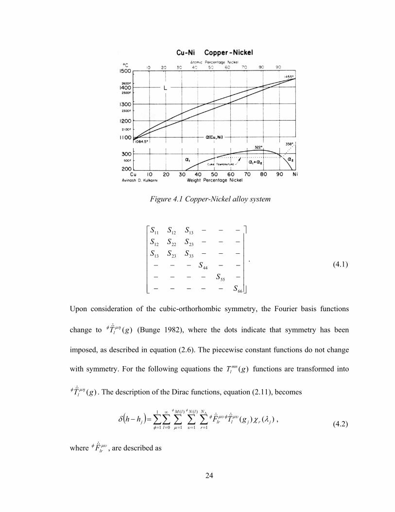
Figure 4.1 Copper-Nickel alloy system
−−−−−−
−−−−−−−−−
−−−−−−−−−
66
55
44
332313
232212
131211
SS
SSSSSSSSSS
. (4.1)
Upon consideration of the cubic-orthorhombic symmetry, the Fourier basis functions
change to (Bunge 1982), where the dots indicate that symmetry has been
imposed, as described in equation (2.6). The piecewise constant functions do not change
with symmetry. For the following equations the T functions are transformed into
. The description of the Dirac functions, equation (2.11), becomes
)(gTlµηφ &&&
)(gmnl
)(gTlµηφ &&&
( ) ∑∑ ∑ ∑ ∑=
∞
= = = =
Λ
=−1
1 0
)(
1
)(
1 1)()(
φ µ υ
µυφµυφφ φ
λχδl
lM lN
jrj
N
rllrj gTFhh &&&&&& , (4.2)
where , are described as µυφlrF&&&
24

)()()()12( *jrjljlr gTMlF λχλ µυφµυφ &&&&&& += . (4.3)
Here enumerates the crystal symmetric subspaces associated with the phase )(lMφ φ
and the index l, and enumerates the sample symmetric subspaces (Bunge (1982),
as tabulated in Figures 4.2 and 4.3
)(lNφ
When symmetry is considered, the local state distribution function, (2.15),
becomes
)()(),,(0
)(
1
)(
1 1
λχλφφ φ
µ υ
µυφµυφr
l
lM lN N
rllr gTFgf ∑ ∑ ∑ ∑
∞
= = = =
Λ
= &&&&&& . (4.4)
changes to (3.16)
∑ ∑ ∑= = =
=4
4,0
)(
1 1
1*1* )()()(l
lN N
rrllrijkm
r
gTijkmDZφ
υ
υφυφφφ λχβ &&&&&& , (4.5)
and (3.17) transforms into
∑ ∑=′ =′
′′
′′=
4
4,0
)(
1
11 )()(l
lN
llrmrkrjri gTijkmDggggφ
υ
υφυφ &&&&&& . (4.6)
Equation (3.18) becomes
∑ ∑ ∑ ∑Λ Λ
= = = =
+=N
r l
lN N
rrllrrrijkm gTijkmDijkmkC
1
4
4,0
)(
1 1
1*1* )()()()()(φ
υ
υφυφφφφ λχβλχ &&&&&& . (4.7)
Looking at the lower bound, (3.29) becomes
∑ ∑ ∑= = =
Λ
=4
4,0
)(
1 1
1*1* )()()(l
lN N
rrllrijkm gTijkmDQ
φ
υ
υφυφφφ λχα &&&&&& , (4.8)
and (3.30) is
∑ ∑ ∑∑= = ==
ΛΛ
+=4
4,0
)(
1 1
1*1*
1)()()()()(
l
lN N
rrllr
N
rrrijkm gTijkmDijkmkS
φ
υ
υφυφφφφ λχαλχ &&&&&& . (4.9)
25

Figure 4.2 Number of linearly independent spherical harmonics of different symmetries as a function of degree l (for even l).
(Bunge1982)
Finally equations (3.19) and (3.31) carry the cubic-orthorhombic symmetry, and for two-
phase examples these become
Figure 4.3 Number of linearly independent spherical harmonics of different symmetries as a function of degree l (for odd l). (Bunge
1982)
26
µφµφφ
φ µ
φ βδφ
11*0
1
1
4
4,0
)(
1 1
* )]()([ lrlrll
lN N
rrijkmijkm FijkmDijkmkCC &&&&&&+=≤ ∑ ∑ ∑ ∑
= = = =
Λ
, (4.10)
1
11*0
1
1
4
0
)(
1 1
1* )]()([−
= = = =
−
+=≥ ∑∑ ∑ ∑
Λµφµφφ
φ µ
φ αδφ
lrlrll
lN N
rrijkmijkm FpqstDpqstkSC &&&&&& . (4.11)
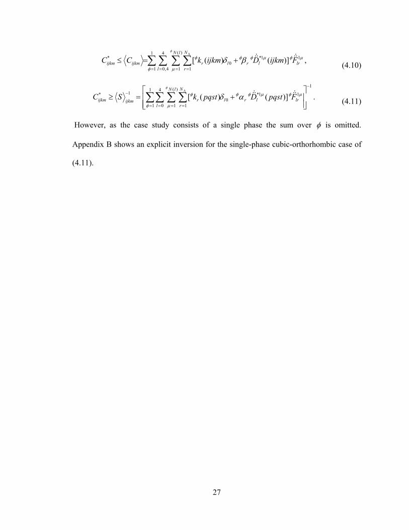
However, as the case study consists of a single phase the sum over φ is omitted.
Appendix B shows an explicit inversion for the single-phase cubic-orthorhombic case of
(4.11).
27

28

5 Elastic Properties in Fourier Space
5.1 Overview
The elastic bounds are expressed as a hyper-plane (4.10) for the upper-bound, and
a hyper-surface (4.11) for the lower-bound on C , within the common spectral
language. These hyper-surfaces translate through the microstructure hull depending on
the selected property value of C . From these translations the extreme property limits
are computed. Additionally these hyper-surfaces are used to identify pockets of
microstructures that fulfill the design objectives.
ijkm*
ijkm*
5.2 Hyper-Surfaces in the Fourier Space
Chapter 2 introduced the microstructure hull which represents all possible
microstructures, expressed by equation (2.16). Points outside the microstructure hull are
fictitious microstructures, having no physical meaning. The hyper-surfaces therefore only
have meaning within the microstructure hull.
A graphical depiction of (4.10) shows that the elastic upper-bound forms hyper-
planes in the multidimensional Fourier space, as shown in Figure 5.1. These hyper-planes
have a set property-bound value for all points that lie upon the plane, i.e. in Figure 5.1 the
plane has a value of 200 GPa. As the hyper-planes are translated through the
spectral representation, property extremes are observed. These extremes are used to
>< 1111C
29

Figure 5.1 Elastic upper-bound of >< 1111C and >< 1212C in the microstructure hull
identify the property closures introduced in Chapter 6. Figure 5.1 shows that each plane
traverses through the microstructure hull with different plane normals. These plane
normals are listed in Table 5.1 for the cubic-orthorhombic case.
Some characteristic of the hyper-planes are that the >< 1111C
124F
144F
hyper-plane yields
higher stiffness values as the plane moves negatively along the axis. < yields
higher stiffness values as the plane translates positively along the axis. Appendix D
contains computer code for calculating points on a set hyper-plane.
>1212C
30
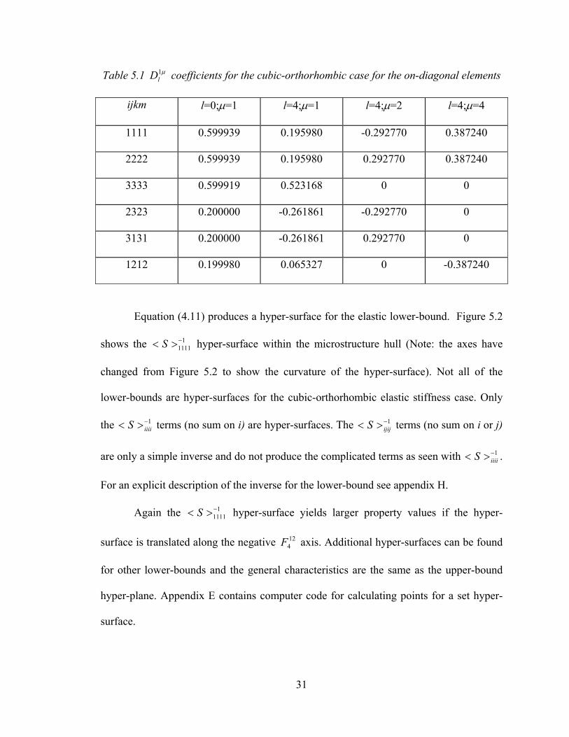
Table 5.1 coefficients for the cubic-orthorhombic case for the on-diagonal elements µ1lD
ijkm l=0;µ=1 l=4;µ=1 l=4;µ=2 l=4;µ=4
1111 0.599939 0.195980 -0.292770 0.387240
2222 0.599939 0.195980 0.292770 0.387240
3333 0.599919 0.523168 0 0
2323 0.200000 -0.261861 -0.292770 0
3131 0.200000 -0.261861 0.292770 0
1212 0.199980 0.065327 0 -0.387240
Equation produces a hyper-surface for the elastic lower-bound. Figure 5.2
shows the hyper-surface within the microstructure hull (Note: the axes have
changed from Figure 5.2 to show the curvature of the hyper-surface). Not all of the
lower-bounds are hyper-surfaces for the cubic-orthorhombic elastic stiffness case. Only
the terms (no sum on i) are hyper-surfaces. The < terms (no sum on i or j)
are only a simple inverse and do not produce the complicated terms as seen with < .
For an explicit description of the inverse for the lower-bound see appendix H.
11111−>< S
1−>< iiiiS 1−> ijijS
1−> iiiiS
(4.11)
Again the < hyper-surface yields larger property values if the hyper-
surface is translated along the negative axis. Additional hyper-surfaces can be found
for other lower-bounds and the general characteristics are the same as the upper-bound
hyper-plane. Appendix E contains computer code for calculating points for a set hyper-
surface.
11111−>S
124F
31

Figure 5.2 Elastic lower-bound of the hyper-surface n the microstructure hull
11111−>< S i
As these hyper-surfaces are added to the microstructure hull, they are used to find
groups of microstructures that fulfill the design objectives. As more design properties are
included, it becomes more difficult to find microstructures that fulfill all design
constraints. Looking at two properties such as C and C , an area of the
microstructure hull is found that satisfies both constraints and is represented as the area in
yellow on Figure 5.3. For C the lower bound < is used, and for the upper
bound is expressed. This area contains multiple microstructures that satisfy the design
constraints chosen by the design engineer..
*1111
*1111>
*1212
*1111 S *
1212C
32
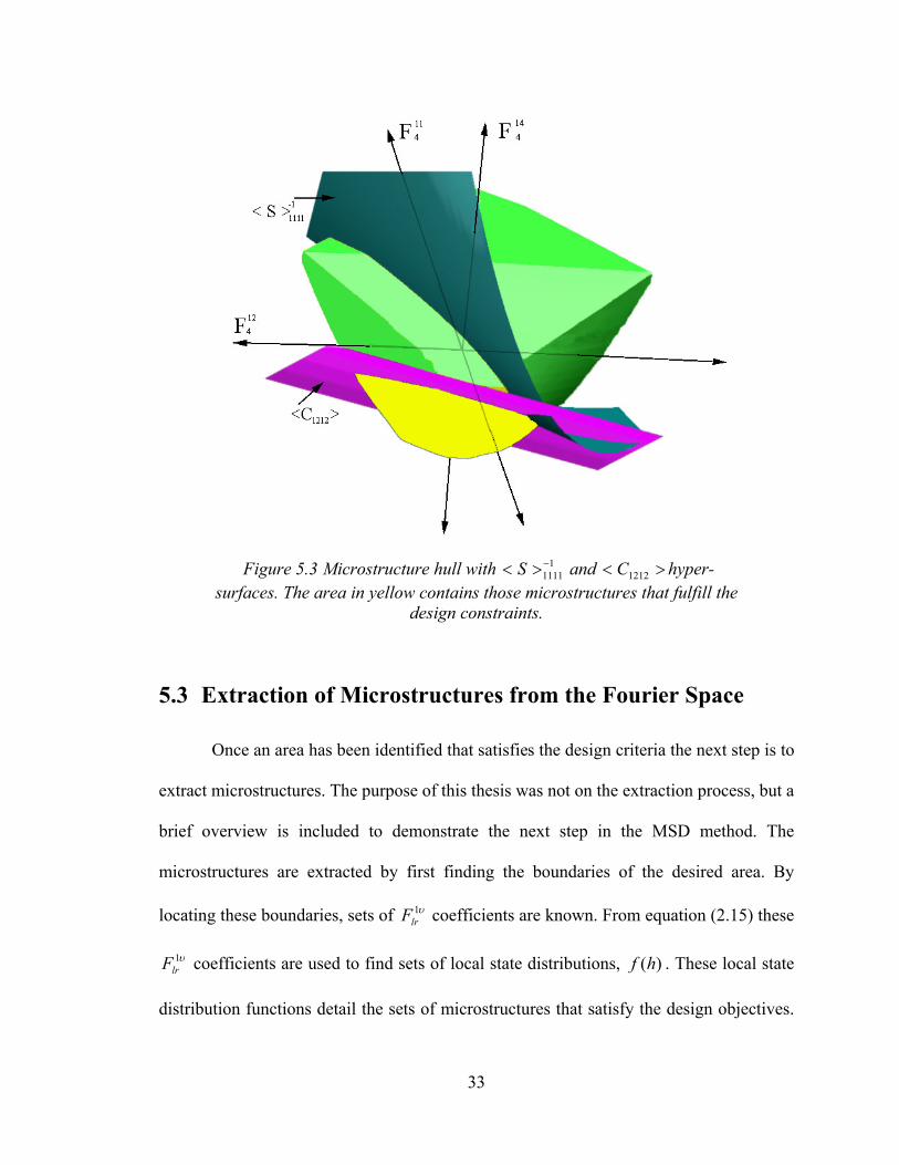
Figure 5.3 Microstructure hull with < and 11111−>S >< 1212C hyper-
surfaces. The area in yellow contains those microstructures that fulfill the design constraints.
5.3 Extraction of Microstructures from the Fourier Space
Once an area has been identified that satisfies the design criteria the next step is to
extract microstructures. The purpose of this thesis was not on the extraction process, but a
brief overview is included to demonstrate the next step in the MSD method. The
microstructures are extracted by first finding the boundaries of the desired area. By
locating these boundaries, sets of coefficients are known. From equation (2.15) these
coefficients are used to find sets of local state distributions, . These local state
distribution functions detail the sets of microstructures that satisfy the design objectives.
υ1lrF
υ1lrF )(hf
33

Figure 5.4 One extracted microstructure that satisfy both the < and 1
1111−>S >< 1212C bounds.
Figure 5.4 shows one microstructure extracted from the yellow area in Figure 5.3. The
constraints associated with the yellow region in Figure 5.3 are described in section 6.3.
34

6 Property Closures
6.1 Overview
Property closures are generated by condensing the information contained within
the multi-dimensional Fourier space into representations of lower-dimensionality (e.g., 2-
D). This compaction of information is beneficial for a quick determination of combined
property limits for a particular alloy system. The property closures are determined by
taking two (or more) property hyper-surfaces found in Chapter 4 through the entire
microstructure hull. From this analysis a closure is formed that encompasses all possible
values for the combined properties. The property closures contain only partial
information from the microstructure hull. The property closures can be used to identify if
there are any microstructures that fulfill the design criteria, but individual microstructures
can only be extracted from the microstructure hull.
6.2 Generation of the Property Closures
For computation of property closures, two properties are selected. These could be
elastic properties or any other property expressed with Fourier coefficients. Only the
upper bound, (4.10), is required for computation of an elastic property closure since the
bounds on elastic properties coincide for single crystalline microstructures, and these
35
occur at the periphery of the microstructure hull, and also at the periphery of the
properties closures.
One approach to generating a 2-D property closure was: one property, i.e. C , is
kept constant while the other property, i.e. , is allowed to move through the
microstructure hull. Since the microstructure hull is calculated from discrete points there
are no formulas for the boundaries. Due to this limitation of the microstructure hull,
another approach was used for generating property closures. The cubic-orthorhombic
orientation space was divided into equal volume boxes. These boxes were then used to
calculate the properties over all orientations, including multiple orientations. From these
calculations the extremes were found by keeping one property constant, i.e. C , and
find the min and max of the second property, i.e. . These extremes form the outer
region of the property closure. Various algorithms can be used since finding the property
closures is simply a min/max problem (Belegundu and Chandrupatla, 1999). For
calculating many property closures, or higher-dimensional closures, a faster algorithm
would be required. Figure 6.1 shows how these extremes are viewed in a 2-D
representation.
*1111
*1111
*1212C
C *1212
6.3 Benefits of the Property Closures
The property closures, used in conjunction with the microstructure hull and the
hyper-surface construction, can identify alloy microstructures that fulfill the selected
design objectives. The design criteria dictates the minimum property values that fulfill
the design objective. These criteria are used to set the effective properties, e.g
property and . For example, if must be greater then 320 GPa, illustrated *1111C *
1212C *1111C
36
Figure 6.1 Property closure of C vs. of the Cu-Ni alloy system *1111
*1212C
by A in Figure 6.2, must be less than 63 GPa, illustrated by B. From Figure 6.2
there is a small area of microstructures that can fulfill both property objectives.
Therefore, it is known that for these two effective properties, sets of microstructures exist
that solve the design objectives. Additional property closures, for the on-diagonal
elements, can be found in Appendix A.
*1212C
Figure 6.2 Property closure of C vs. with design constraints added at A and B
*1111
*1212C
37

38

7 Conclusions and Recommendations
7.1 Conclusions
Through the use of MSD a method of communication between the Design
Engineer, Material Scientist, and Materials Manufacturing Specialist (Processor) has
been developed. This common language allows the design criteria to dictate what
properties are improved, instead of the Material Scientist and Processor guessing what
properties will be of importance. The Fourier space yields sets of solutions that can
include both single and polycrystalline materials. These polycrystalline solutions yield
less expensive solutions compared to single crystal solutions.
The property closures contain only partial information from the microstructure
hull. The property closures can be used to identify if there are any microstructures that
fulfill the design criteria, but individual microstructures can only be extracted from the
microstructure hull. Through this combination of MSD tools difficult design problems
may be solved for multiple design constraints.
The process of transforming properties into the spectral representation is
mathematically intensive, but once this process has been achieved the properties can be
employed to solve a multitude of design problems. For design problems of equal local
state variables, the spectral representation remains the same.
39

7.2 Recommendations
The Hill bounds were used to find the effective stiffness tensor; for the Hill
bounds the variance from actual results is large compared to the elastic bounds recovered
from two-point statistics (Mason, 1999). Hill bounds may be used for design work, but
there is a significant spread of results from the upper and lower bounds. By using the
two-point statistics this spread is greatly reduced and more accurate results can be
achieved. The two-point statistics are realized through Green’s functions. These Green’s
functions increase the degree of difficultly in transforming the bounds, but the additional
accuracy may be sufficient to warrant the effort.
The off diagonal elements of the effective stiffness tensor are required in some
design problems. It is known that these elements have a coupling with the diagonal
elements (Cherkaev, 2000). A better understanding of this coupling and how to recover
the off diagonal elements is of importance.
As design problems leave the simple case of cubic-orthorhombic symmetry the
dimensionality of the Fourier space increases dramatically. Therefore optimization
routines are required for solving multiple design criteria in 10, 50, or an even larger
number of Fourier dimensions.
40
References
Adams, B. L., Henrie, A., Henrie, B., Lyon, M., Kalidindi, S. R., Garmestani, H. (2001)
Microstructure-Sensitive Design of a Compliant Beam, Journal of Mechanics and
Physics of Solids, 49:1639-1663.
Adams, B. L., Olsen T. (1998) The mesostructure-properties linkage in polycrystals,
Progress in Material Science, 43:1-88.
Ashby, M. F. (1992) Materials Selection in Mechanical Design, Pergamon Press Inc.,
New York.
Belegundu, A. D., Chandrupatla, T. R. (1999), Optimization Concepts and Applications
in Engineering, Prentice-Hall, Inc, New Jersy.
Beran, M. J., Mason, T. A., Adams, B. L., and Olson, T. (1996) Bounding elastic
constants of an orthotropic polycrystal from measurements of the microstructure,
Journal of Mechanics and Physics of Solids, 44:1543-63.
Bunge, H. J. (1982) Texture Analysis in Materials Science, Butterworths, London.
Cherkaev, A. (2000) Variational Methods for structural optimization, Springer, New
York.
Courant, R., and Hilbert, D. (1989) Methods of Mathematical Physics, Willey-Inter-
science, New York.
Hartley, C. S. (2001) Single Crystal Elastic Module of Disordered Cubic Alloys Part I:
Face-Centered Cubic Systems, Submitted for publication.
Hashin, Z., and Shtrikman, S. (1962a) On some Variational Principles in Anisotropic and
Nonhomogeneous Elasticity, J. Mech. Phy. Solids, 10: 335-342.
41

Hashin, Z., and Shtrikman, S. (1962b) A Variational Approach to the Theory of the
Elastic Behavior of Polycrystals, J. Mech. Phy. Solids, 10: 343-352.
Hill, R. (1952) The Elastic Behavior of a Crystalline Aggregate, Proc. Phys. Soc. Lond.,
A 65: 349-354.
Hirth, J. P. and Lothe, J. (1968) Theory of Dislocations, McGraw-Hill, Inc.
Howell, L.L., (2001) Compliant Mechanisms, Wiley-Interscience.
Keener, J. P., (2000) Principles of Applied Mathematics, 2nd Ed., Perseus, Cambridge,
Mass.
Knocks, U. F., Tome, C. N., and Wenk H.-R. (1998) Texture and Anisotropy, Cambridge
University Press.
Larsen, U. D., Sigmund, O., and Bouwstra, S. (1997) Design and Fabrication of Compli-
ant Micromechanisms and Structures with Negative Poisson’s Ratio, Journal of
Microelectromechanical Systems, Vol 6, No 2: 99-106.
Mason, T. A., and Adams, B. L., (1999) Use of Microstructural Statistics in Predicting
Polycrystalline Material Properties, Metturgical and Materials Transaction A,
30A:969-79.
Massalski, T. B. (1986), Binary Alloy Phase Diagrams, American Society for Metals.
Olhoff, N., Ronholt, E., and Scheel, J. (1998) Topology Optimization of Three-Dimen-
sional Structures using Optimum Microstructures, Structural Optimization, 16: 1-18.
Olsen, G. B. (1998) System design of hierarchically structured materials: Advanced
steels, Journal of computer-aided materials design, Vol 4, issue 3 143-156.
Reuss, A. (1929) Z. Angew. Math. Mech., 9: 49-58.
Sigmund, O., Torquato, S., and Aksay, I. A. (1998) On the Design of 1-3
Piezocomposites using Topology Optimization, J. Mater. Res. 13: 1038-1048.
Strayer, J. K. (1989) Linear Programming and Its Applications, Springer-Verlag New
York Inc.
42

Subbarayan, G., and Raj, R. (1999) A Methodology for Integrating Materials Science
with System Engineering, Materials and Design, 20: 1-12.
Voigt, W. (1928) Lehrbuch der Kristallphysik, Teubner, Leipzig.
43

44

Appendix
Appendix A : Property Closures The following property closures are for the Cu-Ni alloy system.
Figure A.1 Property closure of s. *1111C v *
2222C
Figure A.2 Property closure of s. *1111C v *
3333C
45

Figure A.3 Property closure of s. *1111C v *
2323C
Figure A.4 Property closure of s. *1111C v *
3131C
46
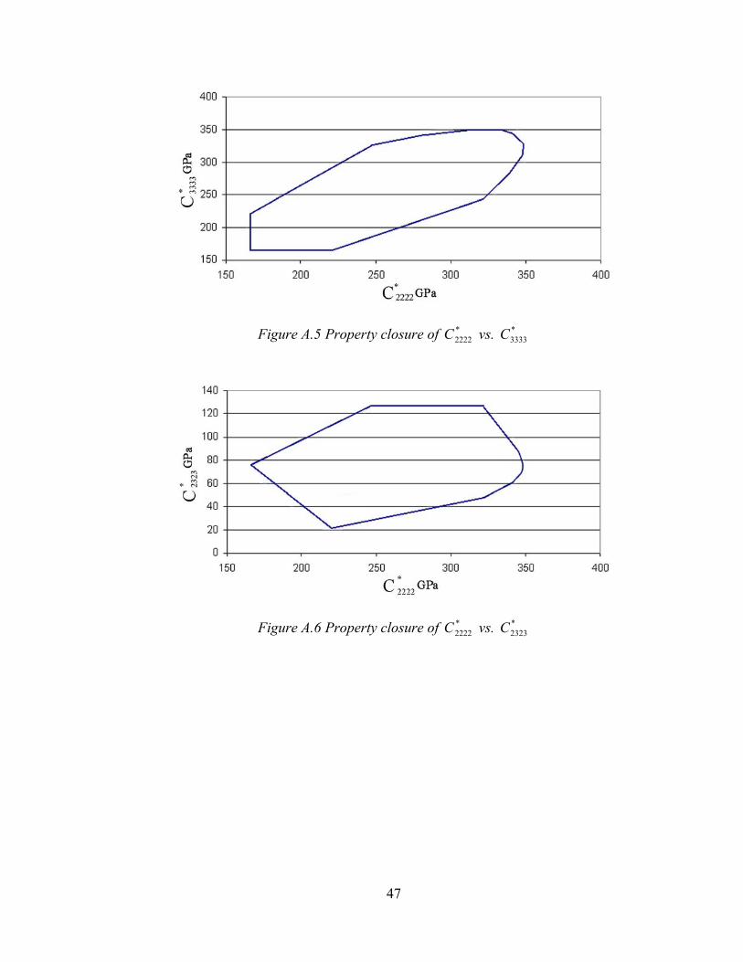
Figure A.5 Property closure of s. *2222C v *
3333C
Figure A.6 Property closure of s. *2222C v *
2323C
47
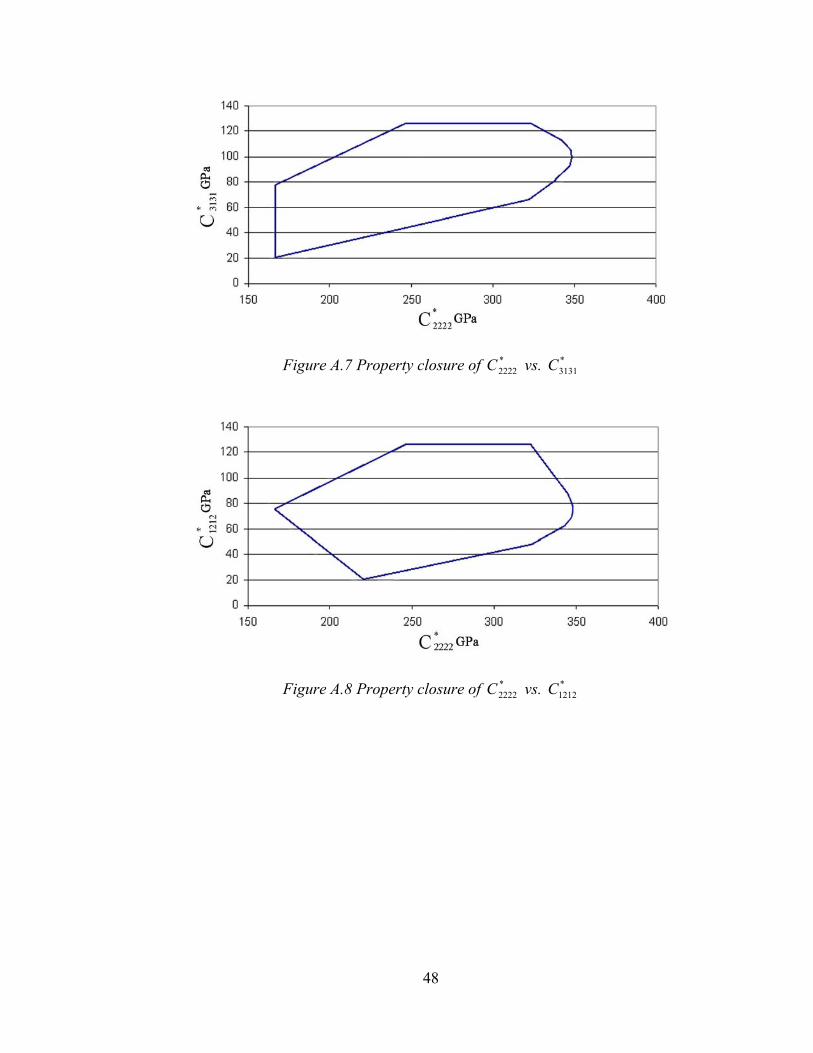
Figure A.7 Property closure of C vs. C *2222
*3131
Figure A.8 Property closure of C vs. C *2222
*1212
48

Figure A.9 Property closure of C vs. C *3333
*2323
Figure A.10 Property closure of s. *3333C v *
3131C
49
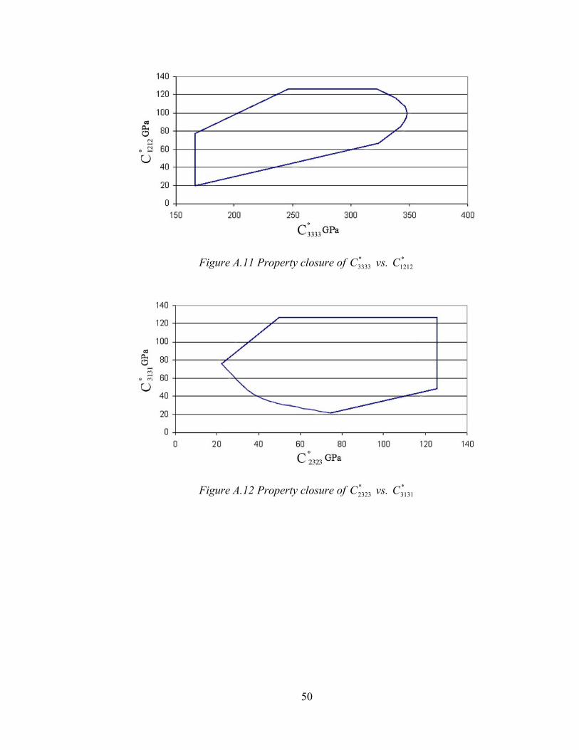
Figure A.11 Property closure of s. *3333C v *
1212C
Figure A.12 Property closure of vs. *2323C *
3131C
50
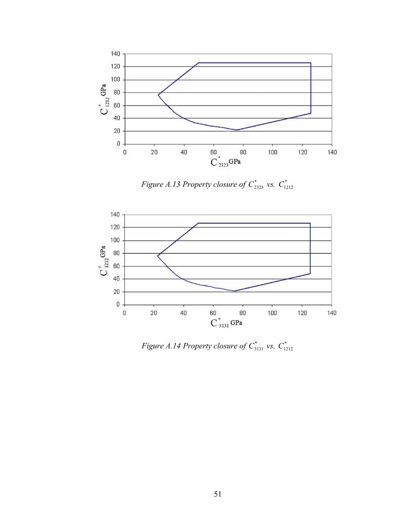
Figure A.13 Property closure of vs. *2323C *
1212C
Figure A.14 Property closure of C vs. C *3131
*1212
51
Appendix B : Inversion for cubic-orthorhombic symmetry The following is an explicit inversion of the ijS ′ tensor to the tensor. From
equation (4.1) the S tensor is
1−′ijS
ij′
′−−−′−−−′
−−−−−−−−−
−−−−−−−−−
′′′′′′′′′
66
55
44
332313
232212
131211
SS
SSSSSSSSSS
. (H.1)
By using cofactors (H.1) is inverted by the following process.
22311
21233
21322231312332211
22333221
11 )()()(2)(
SSSSSSSSSSSSSSS
S′′−′′−′′−′′′+′′′
′−′′=′− (H.2)
22311
21233
21322231312332211
21333111
22 )()()(2)(
SSSSSSSSSSSSSSS
S′′−′′−′′−′′′+′′′
′−′′=′− (H.3)
22311
21233
21322231312332211
21222111
33 )()()(2)(
SSSSSSSSSSSSSSSS
′′−′′−′′−′′′+′′′′−′′
=′− (H.4)
22311
21233
21322231312332211
23131233112 )()()(2 SSSSSSSSSSSS
SSSSS
′′−′′−′′−′′′+′′′′′+′′−
=′− (H.5)
22311
21233
21322231312332211
13222312113 )()()(2 SSSSSSSSSSSS
SSSSS
′′−′′−′′−′′′+′′′′′−′′
=′− (H.6)
52

22311
21233
21322231312332211
13122311123 )()()(2 SSSSSSSSSSSS
SSSSS
′′−′′−′′−′′′+′′′′′+′′−
=′− (H.7)
44
144
1S
S′
=′− (H.8)
55
155
1S
S′
=′− (H.9)
66
166
1S
S′
=′− (H.10)
As can be seen equations (H.8), (H.9), and (H.10) are only a simple inverse and therefore
produce a hyper-plane, and not a hyper-surface such as (H.2), (H.3), and (H.4).
53

Appendix C :Program for generation of the property closures Property_C.c /* property closer of <Cijkm> for the cubic orthorombic symmetry case , but only for Ciiii and Cijij This program used a tie-line method for the material constants, but only a small changed was made to use discrete points from Hartley (). */ #include<stdio.h> #include<stdlib.h> #include<math.h> #include<string.h> #include"property.h" /* these are where is is set which property closure to make */ #define C1 "C1111" #define G1 "g1111" #define K1 C1111 #define g1 g1111 #define C2 "C1212" #define G2 "g1212" #define K2 C1212 #define g2 g1212 #define PI 3.1415926 #define step PI / 25.0 #define N 1 #define ofiles "hartley_base.txt" FILE *outfile; void main() { /********************************************************************** Initalize all variables *************************************************************************/ int I = 1, J = 1, K = 1, M = 2, count = 0; double Land[N+3], landdumb, Ms, aa, bb; /* these are in dynes/cm^2 */ /*double C111 = 1.684e12, C112 = 1.214e12, C144 = 0.754e12; double C211 = 2.465e12, C212 = 1.473e12, C244 = 1.247e12;*/ /* these are in GPa */ double C111 = 168.4, C112 = 121.4, C144 = 75.4; /* copper */ double C211 = 246.5, C212 = 147.3, C244 = 124.7; /* nickel */ double C1111, C2222, C3333, C2323, C3131, C1212, C1122, C1133, C2233; double a1111, a2222, a3333, a2323, a3131, a1212, a1122, a1133, a2233; double b1111, b2222, b3333, b2323, b3131, b1212, b1122, b1133, b2233; double g1111, g2222, g3333, g2323, g3131, g1212, g1122, g1133, g2233; double phi1, PHI, phi2; int pp, p, r; /*********************************************************************** Open the output file and getGs loads in the orientations for a cubic euler space **********************************************************************/ outfile = fopen(ofiles, "w");
54

/********************************************************************** Compute the composition variable by compostition diversion set by N ***********************************************************************/ Ms = 1.0 / N; Land[1] = Ms / 2.0; Land[0] = 0.0; landdumb = Land[1]; for(pp = 2; pp < N + 1; pp++) { landdumb = landdumb + Ms; Land[pp] = landdumb; } Land[N+1] = 1.0; /*********************************************************************
Compute the variables that don't change with composition or orientation **********************************************************************/ a1111 = Aijkm(1,1,1,1,C112,C144); a2222 = Aijkm(2,2,2,2,C112,C144); a3333 = Aijkm(3,3,3,3,C112,C144); a2323 = Aijkm(2,3,2,3,C112,C144); a3131 = Aijkm(3,1,3,1,C112,C144); a1212 = Aijkm(1,2,1,2,C112,C144); a1122 = Aijkm(1,1,2,2,C112,C144); a1133 = Aijkm(1,1,3,3,C112,C144); a2233 = Aijkm(2,2,3,3,C112,C144); b1111 = Bijkm(1,1,1,1,C112,C144,C212,C244); b2222 = Bijkm(2,2,2,2,C112,C144,C212,C244); b3333 = Bijkm(3,3,3,3,C112,C144,C212,C244); b2323 = Bijkm(2,3,2,3,C112,C144,C212,C244); b3131 = Bijkm(3,1,3,1,C112,C144,C212,C244); b1212 = Bijkm(1,2,1,2,C112,C144,C212,C244); b1122 = Bijkm(1,1,2,2,C112,C144,C212,C244); b1133 = Bijkm(1,1,3,3,C112,C144,C212,C244); b2233 = Bijkm(2,2,3,3,C112,C144,C212,C244); aa = C111 - C112 - (2.0 * C144); bb = C211 - C111 + C112 - C212 + (2.0 * C144) - (2.0 * C244); fprintf(outfile, "%s \t %s \t phi1 \t PHI \t phi2 \t %s \t %s \n",C1,C2,G1,G2); /*********************************************************************
Find the minimum & maximum values for a set Ckmkm (which is the Y axes on the property closure)
********************************************************************/ for(p = 0; p < N + 2; p++) { for(phi1 = 0.0001; phi1 <= 2 * PI; phi1+= step) {
for(PHI = 0.0001; PHI <= PI / 2.0; PHI+= step) { for(phi2 = 0.0001; phi2 <= PI / 2.0; phi2+= step) { C1111 = 0.0; C2222 = 0.0; C3333 = 0.0; C2323 = 0.0; C3131 = 0.0; C1212 = 0.0; C1122 = 0.0; C1133 = 0.0; C2233 = 0.0; g1111 = 0.0; g2222 = 0.0; g3333 = 0.0; g2323 = 0.0; g3131 = 0.0; g1212 = 0.0; g1122 = 0.0; g1133 = 0.0; g2233 = 0.0; /**************************************************************** This for loop calculates a value of Ckmkm ************************************************************/ for(r = 1; r < 4; r++) {
55
C1111 += (aa + bb * Land[p]) * Gir(1,r,phi1,PHI,phi2) * Gir(1,r,phi1,PHI,phi2) * Gir(1,r,phi1,PHI,phi2) * Gir(1,r,phi1,PHI,phi2); C2222 += (aa + bb * Land[p]) * Gir(2,r,phi1,PHI,phi2) * Gir(2,r,phi1,PHI,phi2) * Gir(2,r,phi1,PHI,phi2) * Gir(2,r,phi1,PHI,phi2); C3333 += (aa + bb * Land[p]) * Gir(3,r,phi1,PHI,phi2) * Gir(3,r,phi1,PHI,phi2) * Gir(3,r,phi1,PHI,phi2) * Gir(3,r,phi1,PHI,phi2); C2323 += (aa + bb * Land[p]) * Gir(2,r,phi1,PHI,phi2) * Gir(3,r,phi1,PHI,phi2) * Gir(2,r,phi1,PHI,phi2) * Gir(3,r,phi1,PHI,phi2); C3131 += (aa + bb * Land[p]) * Gir(3,r,phi1,PHI,phi2) * Gir(1,r,phi1,PHI,phi2) * Gir(3,r,phi1,PHI,phi2) * Gir(1,r,phi1,PHI,phi2); C1212 += (aa + bb * Land[p]) * Gir(1,r,phi1,PHI,phi2) * Gir(2,r,phi1,PHI,phi2) * Gir(1,r,phi1,PHI,phi2) * Gir(2,r,phi1,PHI,phi2); C1122 += (aa + bb * Land[p]) * Gir(1,r,phi1,PHI,phi2) * Gir(1,r,phi1,PHI,phi2) * Gir(2,r,phi1,PHI,phi2) * Gir(2,r,phi1,PHI,phi2); C1133 += (aa + bb * Land[p]) * Gir(1,r,phi1,PHI,phi2) * Gir(1,r,phi1,PHI,phi2) * Gir(3,r,phi1,PHI,phi2) * Gir(3,r,phi1,PHI,phi2); C2233 += (aa + bb * Land[p]) * Gir(2,r,phi1,PHI,phi2) * Gir(2,r,phi1,PHI,phi2) * Gir(3,r,phi1,PHI,phi2) * Gir(3,r,phi1,PHI,phi2); g1111 += Gir(1,r,phi1,PHI,phi2) * Gir(1,r,phi1,PHI,phi2) * Gir(1,r,phi1,PHI,phi2) * Gir(1,r,phi1,PHI,phi2); g2222 += Gir(2,r,phi1,PHI,phi2) * Gir(2,r,phi1,PHI,phi2) * Gir(2,r,phi1,PHI,phi2) * Gir(2,r,phi1,PHI,phi2); g3333 += Gir(3,r,phi1,PHI,phi2) * Gir(3,r,phi1,PHI,phi2) * Gir(3,r,phi1,PHI,phi2) * Gir(3,r,phi1,PHI,phi2); g2323 += Gir(2,r,phi1,PHI,phi2) * Gir(3,r,phi1,PHI,phi2) * Gir(2,r,phi1,PHI,phi2) * Gir(3,r,phi1,PHI,phi2); g3131 += Gir(3,r,phi1,PHI,phi2) * Gir(1,r,phi1,PHI,phi2) * Gir(3,r,phi1,PHI,phi2) * Gir(1,r,phi1,PHI,phi2); g1212 += Gir(1,r,phi1,PHI,phi2) * Gir(2,r,phi1,PHI,phi2) * Gir(1,r,phi1,PHI,phi2) * Gir(2,r,phi1,PHI,phi2); g1122 += Gir(1,r,phi1,PHI,phi2) * Gir(1,r,phi1,PHI,phi2) * Gir(2,r,phi1,PHI,phi2) * Gir(2,r,phi1,PHI,phi2); g1133 += Gir(1,r,phi1,PHI,phi2) * Gir(1,r,phi1,PHI,phi2) * Gir(3,r,phi1,PHI,phi2) * Gir(3,r,phi1,PHI,phi2); g2233 += Gir(2,r,phi1,PHI,phi2) * Gir(2,r,phi1,PHI,phi2) * Gir(3,r,phi1,PHI,phi2) * Gir(3,r,phi1,PHI,phi2); } C1111 += a1111 + b1111 * Land[p]; C2222 += a2222 + b2222 * Land[p]; C3333 += a3333 + b3333 * Land[p]; C2323 += a2323 + b2323 * Land[p]; C3131 += a3131 + b3131 * Land[p]; C1212 += a1212 + b1212 * Land[p]; C1122 += a1122 + b1122 * Land[p]; C1133 += a1133 + b1133 * Land[p]; C2233 += a2233 + b2233 * Land[p]; ++count; fprintf(outfile,"%lf\t %lf\t %lf\t %lf\t %lf\t %lf\t %lf\n",K1, K2,phi1,PHI,phi2, g1, g2); } } } fprintf(stderr,"%i\n", p); } return; }
56

Appendix D : Program for generation of the upper-bound Upper.c
/* This program finds the hyperplanes for <Cijkm> */ #include<stdio.h> #include<stdlib.h> #include<math.h> #include<string.h> #include"property.h" #define I 1 #define J 1 #define K 1 #define M 1 /* Set this value to find the hyperplane */ #define Cijkm 23.0e11 #define step 0.5 /* output files */ #define xfiles "C1111_x_23.txt" #define yfiles "C1111_y_23.txt" #define zfiles "C1111_z_23.txt" #define ofiles "C1111_23 .txt" FILE *xoutfile; FILE *youtfile; FILE *zoutfile; FILE *outfile; void main() { /* variabels */ double D1111[5][4],D2222[5][4],D3333[5][4],D1122[5][4],D1133[5][4],D2233[5][4],D2323[5][4], D3131[5][4],D1212[5][4]; double D[5][4], F411, F412, F413; double Kijkm, aa; /* These are for copper and are in dynes/cm^2 */ double C111 = 16.84e11, C112 = 12.14e11, C144 = 7.54e11; /* these are for Nickel and are in dynes/cm^2 */ /* double C111 = 24.65e11, C112 = 14.73e11, C144 = 12.47e11; */ /* dummy variables */ int r = 0; /* open files */ xoutfile = fopen(xfiles, "w"); youtfile = fopen(yfiles, "w"); zoutfile = fopen(zfiles, "w"); outfile = fopen(ofiles, "w"); fprintf(stderr,"C%i%i%i%i\n",I,J,K,M); /* input the D coefficients that don't change with composition of same phase FCC */ D1111[0][1]= 0.599939; D1111[4][1]= 0.195980; D1111[4][2]= -0.292770; D1111[4][3]= 0.387240; D2222[0][1]= 0.599939; D2222[4][1]= 0.195980; D2222[4][2]= 0.292770; D2222[4][3]= 0.387240; D3333[0][1]= 0.599919; D3333[4][1]= 0.523168; D3333[4][2]= 0.000000; D3333[4][3]= 0.000000; D1122[0][1]= 0.199980; D1122[4][1]= 0.065327; D1122[4][2]= 0.000000; D1122[4][3]= -0.387240; D1133[0][1]= 0.200000; D1133[4][1]= -0.261861; D1133[4][2]= 0.292770; D1133[4][3]= 0.000000; D2233[0][1]= 0.200000; D2233[4][1]= -0.261861; D2233[4][2]= -0.292770; D2233[4][3]= 0.00000; D2323[0][1]= 0.200000; D2323[4][1]= -0.261861; D2323[4][2]= -0.292770; D2323[4][3]= 0.00000; D3131[0][1]= 0.200000; D3131[4][1]= -0.261861; D3131[4][2]= 0.292770; D3131[4][3]= 0.000000; D1212[0][1]= 0.199980; D1212[4][1]= 0.065327; D1212[4][2]= 0.000000; D1212[4][3]= -0.387240;
57
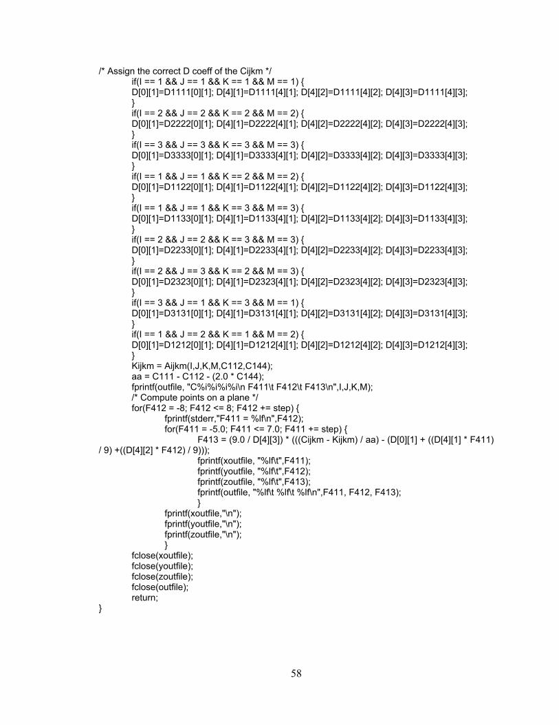
/* Assign the correct D coeff of the Cijkm */ if(I == 1 && J == 1 && K == 1 && M == 1) { D[0][1]=D1111[0][1]; D[4][1]=D1111[4][1]; D[4][2]=D1111[4][2]; D[4][3]=D1111[4][3]; } if(I == 2 && J == 2 && K == 2 && M == 2) { D[0][1]=D2222[0][1]; D[4][1]=D2222[4][1]; D[4][2]=D2222[4][2]; D[4][3]=D2222[4][3]; } if(I == 3 && J == 3 && K == 3 && M == 3) { D[0][1]=D3333[0][1]; D[4][1]=D3333[4][1]; D[4][2]=D3333[4][2]; D[4][3]=D3333[4][3]; } if(I == 1 && J == 1 && K == 2 && M == 2) { D[0][1]=D1122[0][1]; D[4][1]=D1122[4][1]; D[4][2]=D1122[4][2]; D[4][3]=D1122[4][3]; } if(I == 1 && J == 1 && K == 3 && M == 3) { D[0][1]=D1133[0][1]; D[4][1]=D1133[4][1]; D[4][2]=D1133[4][2]; D[4][3]=D1133[4][3]; } if(I == 2 && J == 2 && K == 3 && M == 3) { D[0][1]=D2233[0][1]; D[4][1]=D2233[4][1]; D[4][2]=D2233[4][2]; D[4][3]=D2233[4][3]; } if(I == 2 && J == 3 && K == 2 && M == 3) { D[0][1]=D2323[0][1]; D[4][1]=D2323[4][1]; D[4][2]=D2323[4][2]; D[4][3]=D2323[4][3]; } if(I == 3 && J == 1 && K == 3 && M == 1) { D[0][1]=D3131[0][1]; D[4][1]=D3131[4][1]; D[4][2]=D3131[4][2]; D[4][3]=D3131[4][3]; } if(I == 1 && J == 2 && K == 1 && M == 2) { D[0][1]=D1212[0][1]; D[4][1]=D1212[4][1]; D[4][2]=D1212[4][2]; D[4][3]=D1212[4][3]; } Kijkm = Aijkm(I,J,K,M,C112,C144); aa = C111 - C112 - (2.0 * C144); fprintf(outfile, "C%i%i%i%i\n F411\t F412\t F413\n",I,J,K,M); /* Compute points on a plane */ for(F412 = -8; F412 <= 8; F412 += step) { fprintf(stderr,"F411 = %lf\n",F412); for(F411 = -5.0; F411 <= 7.0; F411 += step) { F413 = (9.0 / D[4][3]) * (((Cijkm - Kijkm) / aa) - (D[0][1] + ((D[4][1] * F411) / 9) +((D[4][2] * F412) / 9))); fprintf(xoutfile, "%lf\t",F411); fprintf(youtfile, "%lf\t",F412); fprintf(zoutfile, "%lf\t",F413); fprintf(outfile, "%lf\t %lf\t %lf\n",F411, F412, F413); } fprintf(xoutfile,"\n"); fprintf(youtfile,"\n"); fprintf(zoutfile,"\n"); } fclose(xoutfile); fclose(youtfile); fclose(zoutfile); fclose(outfile); return; }
58
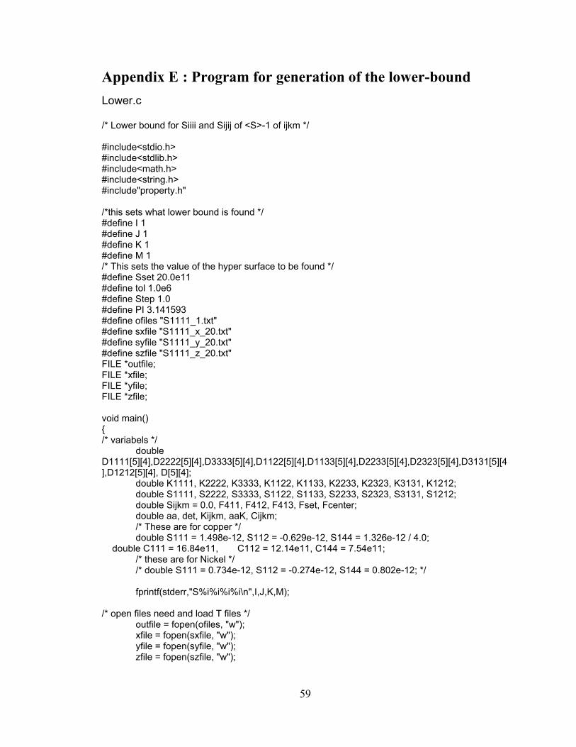
Appendix E : Program for generation of the lower-bound Lower.c
/* Lower bound for Siiii and Sijij of <S>-1 of ijkm */ #include<stdio.h> #include<stdlib.h> #include<math.h> #include<string.h> #include"property.h" /*this sets what lower bound is found */ #define I 1 #define J 1 #define K 1 #define M 1 /* This sets the value of the hyper surface to be found */ #define Sset 20.0e11 #define tol 1.0e6 #define Step 1.0 #define PI 3.141593 #define ofiles "S1111_1.txt" #define sxfile "S1111_x_20.txt" #define syfile "S1111_y_20.txt" #define szfile "S1111_z_20.txt" FILE *outfile; FILE *xfile; FILE *yfile; FILE *zfile; void main() { /* variabels */ double D1111[5][4],D2222[5][4],D3333[5][4],D1122[5][4],D1133[5][4],D2233[5][4],D2323[5][4],D3131[5][4],D1212[5][4], D[5][4]; double K1111, K2222, K3333, K1122, K1133, K2233, K2323, K3131, K1212; double S1111, S2222, S3333, S1122, S1133, S2233, S2323, S3131, S1212; double Sijkm = 0.0, F411, F412, F413, Fset, Fcenter; double aa, det, Kijkm, aaK, Cijkm; /* These are for copper */ double S111 = 1.498e-12, S112 = -0.629e-12, S144 = 1.326e-12 / 4.0; double C111 = 16.84e11, C112 = 12.14e11, C144 = 7.54e11; /* these are for Nickel */ /* double S111 = 0.734e-12, S112 = -0.274e-12, S144 = 0.802e-12; */ fprintf(stderr,"S%i%i%i%i\n",I,J,K,M); /* open files need and load T files */ outfile = fopen(ofiles, "w"); xfile = fopen(sxfile, "w"); yfile = fopen(syfile, "w"); zfile = fopen(szfile, "w");
59
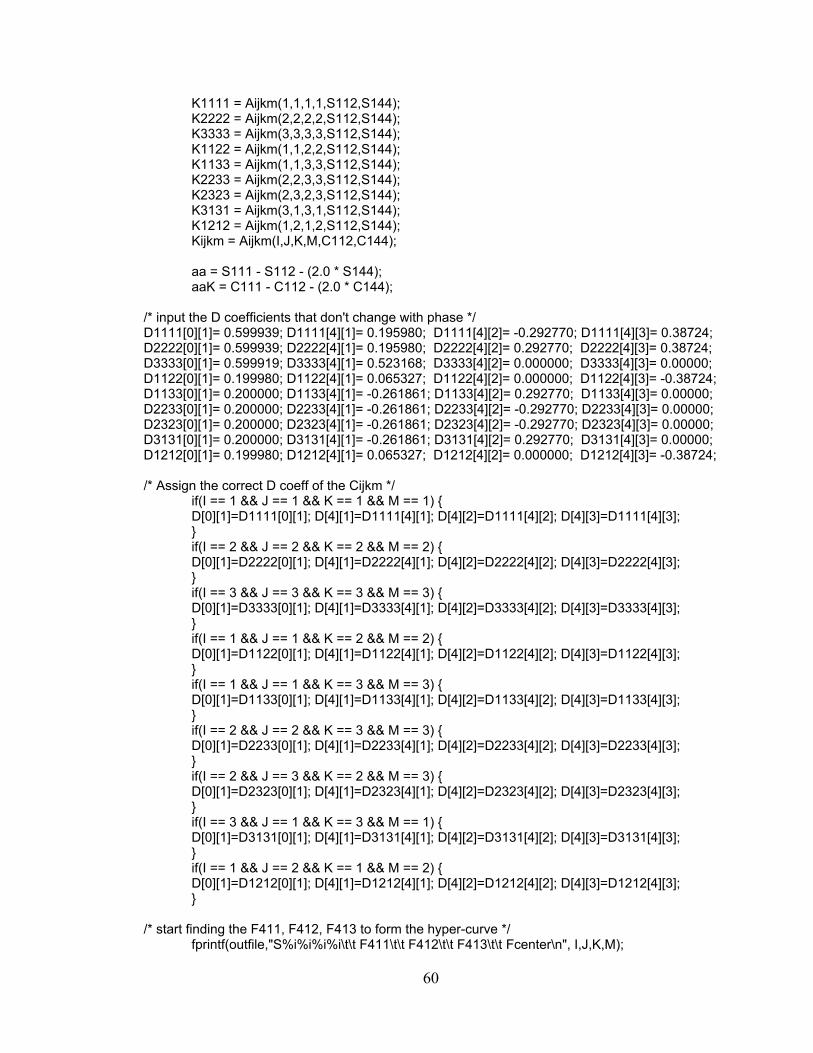
K1111 = Aijkm(1,1,1,1,S112,S144); K2222 = Aijkm(2,2,2,2,S112,S144); K3333 = Aijkm(3,3,3,3,S112,S144); K1122 = Aijkm(1,1,2,2,S112,S144); K1133 = Aijkm(1,1,3,3,S112,S144); K2233 = Aijkm(2,2,3,3,S112,S144); K2323 = Aijkm(2,3,2,3,S112,S144); K3131 = Aijkm(3,1,3,1,S112,S144); K1212 = Aijkm(1,2,1,2,S112,S144); Kijkm = Aijkm(I,J,K,M,C112,C144); aa = S111 - S112 - (2.0 * S144); aaK = C111 - C112 - (2.0 * C144); /* input the D coefficients that don't change with phase */ D1111[0][1]= 0.599939; D1111[4][1]= 0.195980; D1111[4][2]= -0.292770; D1111[4][3]= 0.38724; D2222[0][1]= 0.599939; D2222[4][1]= 0.195980; D2222[4][2]= 0.292770; D2222[4][3]= 0.38724; D3333[0][1]= 0.599919; D3333[4][1]= 0.523168; D3333[4][2]= 0.000000; D3333[4][3]= 0.00000; D1122[0][1]= 0.199980; D1122[4][1]= 0.065327; D1122[4][2]= 0.000000; D1122[4][3]= -0.38724; D1133[0][1]= 0.200000; D1133[4][1]= -0.261861; D1133[4][2]= 0.292770; D1133[4][3]= 0.00000; D2233[0][1]= 0.200000; D2233[4][1]= -0.261861; D2233[4][2]= -0.292770; D2233[4][3]= 0.00000; D2323[0][1]= 0.200000; D2323[4][1]= -0.261861; D2323[4][2]= -0.292770; D2323[4][3]= 0.00000; D3131[0][1]= 0.200000; D3131[4][1]= -0.261861; D3131[4][2]= 0.292770; D3131[4][3]= 0.00000; D1212[0][1]= 0.199980; D1212[4][1]= 0.065327; D1212[4][2]= 0.000000; D1212[4][3]= -0.38724; /* Assign the correct D coeff of the Cijkm */ if(I == 1 && J == 1 && K == 1 && M == 1) { D[0][1]=D1111[0][1]; D[4][1]=D1111[4][1]; D[4][2]=D1111[4][2]; D[4][3]=D1111[4][3]; } if(I == 2 && J == 2 && K == 2 && M == 2) { D[0][1]=D2222[0][1]; D[4][1]=D2222[4][1]; D[4][2]=D2222[4][2]; D[4][3]=D2222[4][3]; } if(I == 3 && J == 3 && K == 3 && M == 3) { D[0][1]=D3333[0][1]; D[4][1]=D3333[4][1]; D[4][2]=D3333[4][2]; D[4][3]=D3333[4][3]; } if(I == 1 && J == 1 && K == 2 && M == 2) { D[0][1]=D1122[0][1]; D[4][1]=D1122[4][1]; D[4][2]=D1122[4][2]; D[4][3]=D1122[4][3]; } if(I == 1 && J == 1 && K == 3 && M == 3) { D[0][1]=D1133[0][1]; D[4][1]=D1133[4][1]; D[4][2]=D1133[4][2]; D[4][3]=D1133[4][3]; } if(I == 2 && J == 2 && K == 3 && M == 3) { D[0][1]=D2233[0][1]; D[4][1]=D2233[4][1]; D[4][2]=D2233[4][2]; D[4][3]=D2233[4][3]; } if(I == 2 && J == 3 && K == 2 && M == 3) { D[0][1]=D2323[0][1]; D[4][1]=D2323[4][1]; D[4][2]=D2323[4][2]; D[4][3]=D2323[4][3]; } if(I == 3 && J == 1 && K == 3 && M == 1) { D[0][1]=D3131[0][1]; D[4][1]=D3131[4][1]; D[4][2]=D3131[4][2]; D[4][3]=D3131[4][3]; } if(I == 1 && J == 2 && K == 1 && M == 2) { D[0][1]=D1212[0][1]; D[4][1]=D1212[4][1]; D[4][2]=D1212[4][2]; D[4][3]=D1212[4][3]; } /* start finding the F411, F412, F413 to form the hyper-curve */ fprintf(outfile,"S%i%i%i%i\t\t F411\t\t F412\t\t F413\t\t Fcenter\n", I,J,K,M);
60

for(F412 = -8.0; F412 <= 8.0; F412 += Step) { fprintf(stderr,"F412 = %lf\n",F412); for(F411 = -6.0; F411 <= 8.0; F411 += Step) { F411 = -0.1447497; F412 = 0.04706759; F413 = -0.2128656; Fcenter = (9.0 / D[4][3]) * (((Sset - Kijkm) / aaK) - (D[0][1] + ((D[4][1] * F411) / 9) +((D[4][2] * F412) / 9))); Cijkm = Kijkm + aaK * (D[0][1] + ((D[4][1] * F411) / 9.0) + ((D[4][2] * F412) / 9.0) + ((D[4][3] * Fcenter) / 9.0)); Fset = Fcenter + 30.0; for(F413 = Fcenter - 30.0; F413 <= Fset; F413 += 0.00001) { F411 = -0.1447497; F412 = 0.04706759; F413 = -0.2128656; S1111 = K1111 + aa * (D1111[0][1] + (D1111[4][1] / 9.0) * F411 + (D1111[4][2] / 9.0) * F412 + (D1111[4][3] / 9.0) * F413); S2222 = K2222 + aa * (D2222[0][1] + (D2222[4][1] / 9.0) * F411 + (D2222[4][2] / 9.0) * F412 + (D2222[4][3] / 9.0) * F413); S3333 = K3333 + aa * (D3333[0][1] + (D3333[4][1] / 9.0) * F411 + (D3333[4][2] / 9.0) * F412 + (D3333[4][3] / 9.0) * F413); S1122 = K1122 + aa * (D1122[0][1] + (D1122[4][1] / 9.0) * F411 + (D1122[4][2] / 9.0) * F412 + (D1122[4][3] / 9.0) * F413); S1133 = K1133 + aa * (D1133[0][1] + (D1133[4][1] / 9.0) * F411 + (D1133[4][2] / 9.0) * F412 + (D1133[4][3] / 9.0) * F413); S2233 = K2233 + aa * (D2233[0][1] + (D2233[4][1] / 9.0) * F411 + (D2233[4][2] / 9.0) * F412 + (D2233[4][3] / 9.0) * F413); S2323 = K2323 + aa * (D2323[0][1] + (D2323[4][1] / 9.0) * F411 + (D2323[4][2] / 9.0) * F412 + (D2323[4][3] / 9.0) * F413); S3131 = K3131 + aa * (D3131[0][1] + (D3131[4][1] / 9.0) * F411 + (D3131[4][2] / 9.0) * F412 + (D3131[4][3] / 9.0) * F413); S1212 = K1212 + aa * (D1212[0][1] + (D1212[4][1] / 9.0) * F411 + (D1212[4][2] / 9.0) * F412 + (D1212[4][3] / 9.0) * F413); /* this is where the inverse is calculated */ det = (S1111 * S2222 * S3333) + (2 * S1122 * S1133 * S2233) - (S2222 * S1133 * S1133) - (S3333 * S1122 * S1122) - (S1111 * S2233 * S2233); /* this is for S1111 */ /* S1111 */ if(I == 1 && J == 1 && K == 1 && M == 1) { Sijkm = ((S2222 * S3333) - (S2233 * S2233)) / det; } /* S2222 */ if(I == 2 && J == 2 && K == 2 && M == 2) { Sijkm = ((S1111 * S3333) - (S1133 * S1133)) / det; } /* S3333 */ if(I == 3 && J == 3 && K == 3 && M == 3) { Sijkm = ((S1111 * S2222) - (S1122 * S1122)) / det; } /* S1122 */ if(I == 1 && J == 1 && K == 2 && M == 2) { Sijkm = ((-1 * S3333 * S1122) + (S1133 * S2233)) / det; } /* S1133 */ if(I == 1 && J == 1 && K == 3 && M == 3) {
61
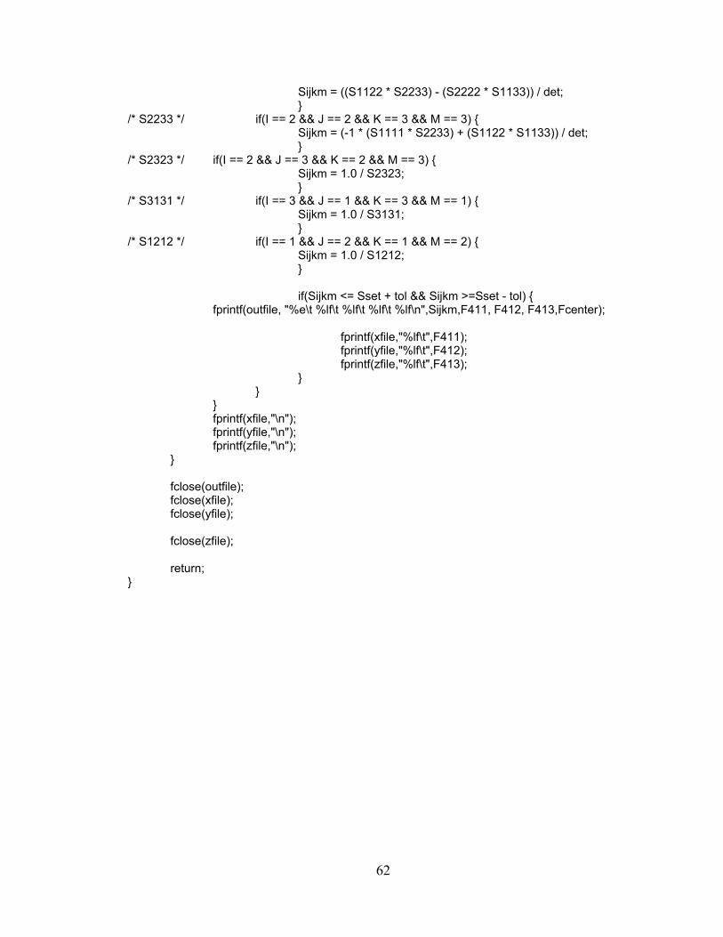
Sijkm = ((S1122 * S2233) - (S2222 * S1133)) / det; } /* S2233 */ if(I == 2 && J == 2 && K == 3 && M == 3) { Sijkm = (-1 * (S1111 * S2233) + (S1122 * S1133)) / det; } /* S2323 */ if(I == 2 && J == 3 && K == 2 && M == 3) { Sijkm = 1.0 / S2323; } /* S3131 */ if(I == 3 && J == 1 && K == 3 && M == 1) { Sijkm = 1.0 / S3131; } /* S1212 */ if(I == 1 && J == 2 && K == 1 && M == 2) { Sijkm = 1.0 / S1212; } if(Sijkm <= Sset + tol && Sijkm >=Sset - tol) { fprintf(outfile, "%e\t %lf\t %lf\t %lf\t %lf\n",Sijkm,F411, F412, F413,Fcenter); fprintf(xfile,"%lf\t",F411); fprintf(yfile,"%lf\t",F412); fprintf(zfile,"%lf\t",F413); } } } fprintf(xfile,"\n"); fprintf(yfile,"\n"); fprintf(zfile,"\n"); } fclose(outfile); fclose(xfile); fclose(yfile); fclose(zfile); return; }
62

Appendix F : Program for computing the coefficients ηφ 1*lrD
D_coeff.c
/* this finds the D coefficients need by the other programs */ #include<stdio.h> #include<stdlib.h> #include<math.h> #include<string.h> #include"property.h" #include"harmonics.h" #define I 1 #define J 1 #define K 1 #define M 1 #define L 4 #define n 3 #define step PI / 100 /* #define PI 3.141593 // from harmonics.h file */ #define ofiles "D_1111.txt" FILE *outfile; void main() { /* variabels */ double D[5][4], test, phi1, phi2, PHI, Gs; double factor; /* dummy variables */ int r; /* open files need and load T files */ outfile = fopen(ofiles, "w"); getFourieras(); getCubicBs(); factor = 1.0 / (8.0 * PI * PI); test = 0.0; D[0][1] = 0.0; D[4][1] = 0.0; D[4][2] = 0.0; D[4][2] = 0.0; for(phi1 = 0.0001; phi1 <= 2 * PI; phi1 += step) { for(PHI = 0.0001; PHI <= PI; PHI += step) { for(phi2 = 0.0001; phi2 <= 2.0 * PI;phi2 +=step) { test += CubLowerT(4,1,n,phi1,PHI,phi2).re * CubLowerT(4,1,n,phi1,PHI,phi2).re * sin(PHI) * factor * (step * step * step); Gs = 0.0; for(r = 1; r < 4; r++) { Gs += Gir(I,r,phi1,PHI,phi2) * Gir(J,r,phi1,PHI,phi2) * Gir(K,r,phi1,PHI,phi2) * Gir(M,r,phi1,PHI,phi2); } D[0][1] += Gs * factor * sin(PHI) * (step * step * step); D[L][1] += Gs * factor * sin(PHI) * (step * step * step) * CubLowerT(L,1,1,phi1,PHI,phi2).re; D[L][2] += Gs * factor * sin(PHI) * (step * step * step) * CubLowerT(L,1,2,phi1,PHI,phi2).re;
63
D[L][3] += Gs * factor * sin(PHI) * (step * step * step) * CubLowerT(L,1,3,phi1,PHI,phi2).re; } } } fprintf(stderr, "T41%i intergration = %lf\n",n,9 * test); /* times in the 2l+1 factor */ D[0][1] = D[0][1] * (2.0 * 0 + 1.0); D[L][1] = D[L][1] * (2.0 * L + 1.0); D[L][2] = D[L][2] * (2.0 * L + 1.0); D[L][3] = D[L][3] * (2.0 * L + 1.0); fprintf(stderr, "D011 = %lf\t D411 = %lf\t D412 = %lf\t D413 = %lf\n",D[0][1],D[L][1],D[L][2],D[L][3]); fprintf(outfile, "C%i%i%i%i D coefficients \n",I,J,K,M); fprintf(outfile, "D011 = %lf\t D411 = %lf\t D412 = %lf\t D413 = %lf\n",D[0][1],D[L][1],D[L][2],D[L][3]); fclose(outfile); return; }
64

Appendix G : Harmonics.h subroutine Harmonics.h
/* ------------------------------------------------------------------------------------ * This library of routines contains functions for calculating an ODF using a * Generalized Spherical Harmonic Series Expansion (GSHE) from single orientation * measurements existing in the form of orientation matrices. Unless otherwise noted * the mathematics for the code are found in: * * H.J. Bunge, Texture Analysis in Materials Science. Butterworths, London (1982) * * Stuart Wright, Yale University (1991). * * Pole Figures routines have been added. The output and inputs for these routines * are formatted according to popLA conventions. * * Stuart Wright, Los Alamos National Lab (1993). * ---------------------------------------------------------------------------------- */ /* ------------------------------------------------------------------------------------ * The U.S. Government is licensed to use, reproduce, and distribute this software. * Permission is granted to the public to copy and use these portions of the software * without charge, provided that this notice and the following statement of authorship * are reproduced in all copies. * * Neither the U.S. Government nor S. I. Wright makes any warranty, express or * implied, or assumes liability or responsibility for the use of this software. * * ---------------------------------------------------------------------------------- */ /* ------------------------------------------------------------------------------------ * The following is an initializing routine required before using any of the * GSHE routines. It returns an error code according to the following: * 0: No errors encounterd. * 1: Invalid symmetry combination. * 2: Problem reading Cubic symmetry coefficients. * 3: Problem reading Fourier Coefficients. * 4: Not enough memory to allocate arrays. * 5: Not enough memory for Taylor Factor calculations. * * cv: Verbose - show error messages * l: Rank for harmonic expansions * Csym: Crystal Symmetry * Psym: Processing, sample or statistical symmetry * EXAMPLE: GSHEInit(1,16,cubic,triclinic) * ---------------------------------------------------------------------------------- */ /* Portions of the above mentioned software is included in the file harmonics.h*/ /* Functions getFourieras(void), getCubicBs(void) -
65

Load tables of values required for all other functions. complex kfnc(int l, int m, double phi, double beta) - Calculates surface spherical harmonic functions without symmetry. double kcbcfnc(int l, int m, double phi, double beta) - Calculates surface spherical harmonic functions with cubic crystal symmetry. complex CubTriclT(int l,int mu,int nu,float phi1,float PHI,float phi2) - This function calculates the T functions with cubic-triclinic symmetry. complex TriLowerT(int l,int mu,int nu,float phi1,float PHI,float phi2) - This function calculates the T functions when the crystal is triclinic and the right-hand symmetry is lower. complex LowerTriT(int l,int mu,int nu,float phi1,float PHI,float phi2) - This function calculates the T functions when the right-hand symmetry is triclinic and the crystal symmetry is lower. complex LowLowerT(int l,int mu,int nu,float phi1,float PHI,float phi2) - This function calculates the T functions when both symmetries are lower. (Bunge eqn. (14.258)). complex CubLowerT(int l,int mu,int nu,float phi1,float PHI,float phi2) - This function calculates the T functions when the processing symmetry is 'low' and the crystal symmetry is 'high' (cubic) (Bunge eqn. (14.261)). complex CubCubicT(int l,int mu,int nu,float phi1,float PHI,float phi2) - This function calculates the T functions cubic-cubic symmetry (Bunge eqn. (14.271)). complex TriTriclT(int l,int mu,int nu,float phi1,float PHI,float phi2) - This function calculates the T functions when both symmetries are triclinic. */ #include<stdio.h> #include<stdlib.h> #include<string.h> #include<time.h> #include<math.h> #define rank 34 #define triclinic 0 #define orthorhombic 11 #define orthotropic 11 #define tetragonal 12 #define hexagonal 13 #define axial 14 #define monoclinic 15 #define trigonal 20 #define cubic 1 #define PI 3.1415926535897931 #define sign(l) (((l)%2) ? -1:1) #define sq2pi 2.506628274631
66
#define sq2 1.414213562373 typedef struct complex { double re; double im; } complex; double B[35][9][4]; double a[35][35][35][35]; char path[200]; double sinPHI[50]; double cosPHI[50]; int processSym,crystalSym, *M,*N ,SymCombo,bsize; /*getFourieras function from GSHELib.c from Stuart Wright*/ /* ------------------------------------------------------------------------------------ * The following function reads in the Fourier coefficients (a'lmns) from file almnsp. * It returns a = 1 if successful. * ---------------------------------------------------------------------------------- */ int getFourieras(void) { FILE *asFile; int l,m,n,s; double almns; /* read in Fourier coefficients from file almnsp */ asFile = fopen("almnsp","r"); if (!asFile) return 0; for (l=0; l<rank; ++l) { for (m=0; m<=l; ++m) for (n=0; n<=m; ++n) for (s=0; s<=l; ++s) { if(fscanf(asFile,"%lf",&almns)==EOF) return(0); a[l][m][n][s] = almns; a[l][n][m][s] = almns; } } fclose(asFile); return 1; } /*getCubicBs function from GSHELib.c from Stuart Wright*/ /* ------------------------------------------------------------------------------------ * The following function reads in the cubic symmetry coefficients (Bl4mn) from file * CubicBs. It returns a = 1 if successful. * ---------------------------------------------------------------------------------- */ int getCubicBs() { FILE *BsFile; int l,m,n; double Blmn; /* read in cubic symmetry coefficients from file CubicBs */ BsFile = fopen("CubicBs","r"); if (!BsFile) return 0; for (;;) {
67

if (fscanf(BsFile,"%i %i %i %lf",&l,&m,&n,&Blmn)==EOF) break; if (l > rank) break; B[l][m][n] = Blmn; } fclose(BsFile); return 1; } double Pfnc(int m, int l, double phi) { int mevent,moddt,s,slevent,sloddt; int m2event,m2oddt; double anpc,asnpc,aspc; double rv; double angl; rv=0; mevent= (m / 2.0) +.1; moddt= (m / 2.0) +.9; if(mevent==moddt) { for(s=0;s<=l;s++) { anpc=a[l][m][0][s]; slevent= ((l+s) / 2.0) +.1; sloddt= ((l+s) / 2.0) +.9; m2event= (m / 4.0) +.1; m2oddt= (m / 4.0) +.9; if(m2event==m2oddt)asnpc= anpc / (sqrt((2.0 / (2 * l + 1)))); if(m2event!=m2oddt)asnpc= (-anpc) / (sqrt((2.0 / (2 * l + 1)))); if(slevent==sloddt)aspc=asnpc; if(slevent!=sloddt)aspc=0; angl=(s * phi); rv+=(aspc * (cos(angl))); } } if(mevent!=moddt) { for(s=0;s<=l;s++) { anpc=a[l][m][0][s]; slevent= ((l+s) / 2.0) +.1; sloddt= ((l+s) / 2.0) +.9; m2event= ((m-1) / 4.0) +.1; m2oddt= ((m-1) / 4.0) +.9; if(m2event==m2oddt)asnpc= (-anpc) / (sqrt((2.0 / (2 * l + 1)))); if(m2event!=m2oddt)asnpc= (anpc) / (sqrt((2.0 / (2 * l + 1)))); if(slevent==sloddt)aspc=asnpc; if(slevent!=sloddt)aspc=0; angl=(s * phi); rv+=(aspc * (sin(angl))); } rv=-rv; } return(rv);
68

} complex kfnc(int l, int m, double phi, double beta) { complex value1,value3; double value2; int me,mo; me=getCubicBs(); mo=getFourieras(); value2=Pfnc(m,l,phi); value1.re=((cos (m * beta)) / sqrt((2 * PI))); value1.im=((sin (m * beta)) / sqrt((2 * PI))); me= (m / 2.0) +.1; mo= (m / 2.0) +.9; if(me==mo) { value3.re=value1.re * value2; value3.im=value1.im * value2; } if(me!=mo) { value3.re=value1.re * value2; value3.im=value1.im * value2; /*value3.re=(-1 * value1.im * value2); value3.im=(value1.re * value2);*/ } return(value3); } double kcbcfnc(int l, int m, double phi, double beta) { int n; double rv; int ne ,no ; rv=0; for(n=0;n<=l;n++) { /*ne = (n / 2.0) +.1; no = (n / 2.0) +.9; if(ne==no) rv.re+=(B[l][n][m] * Pfnc(n,l,phi) * cos((n * beta))); if(ne!=no) rv.im+=(B[l][n][m] * Pfnc(n,l,phi) * cos((n * beta)));*/ ne= ((n) / 4.0) + .1; no= ((n) / 4.0) + .9; if(ne==no) rv+=(B[l][ne][m] * Pfnc(n,l,phi) * cos((n * beta))); } return(rv); } /* ------------------------------------------------------------------------------------ * This function calculates the T functions cubic-triclinic symmetry. * ---------------------------------------------------------------------------------- */ complex CubTriclT(int l,int mu,int nu,float phi1,float PHI,float phi2) {
69
complex Tlmn,R; int m,s; float cc,cs,ss,sc,cnp1,snp1,cmp2,smp2; double sum1,sum2; double sinPHI[50]; double cosPHI[50]; Tlmn.re = 1; Tlmn.im = 0; if (l==0) return Tlmn; /* --- Attempt to speed up calculations --- */ Tlmn.im = Tlmn.re = 0; cnp1 = (float) cos(nu * phi1); snp1 = (float) sin(nu * phi1); if ((nu%2)!=0) { for (s=1; s<=l; ++s) sinPHI[s] = sin(s * PHI); for (m=0; m<=l; m+=4) { sum1 = sum2 = 0.0; cmp2 = (float) cos(m * phi2); smp2 = (float) sin(m * phi2); cc = cmp2 * cnp1; ss = smp2 * snp1; sc = smp2 * cnp1; cs = cmp2 * snp1; for (s=2; s<=l; s+=2) sum1 += a[l][m][nu][s] * sinPHI[s]; for (s=1; s<=l; s+=2) sum2 += a[l][m][nu][s] * sinPHI[s]; R.re = -cs * sum1 -sc * sum2; R.im = cc * sum1 - ss * sum2; Tlmn.re += (B[l][m/4][mu] * R.re); Tlmn.im += (B[l][m/4][mu] * R.im); } } else { for (s=0; s<=l; ++s) cosPHI[s] = cos(s * PHI); for (m=0; m<=l; m+=4) { sum1 = sum2 = 0.0; cmp2 = (float) cos(m * phi2); smp2 = (float) sin(m * phi2); cc = cmp2 * cnp1; ss = smp2 * snp1; sc = smp2 * cnp1;
70
cs = cmp2 * snp1; for (s=0; s<=l; s+=2) sum1 += a[l][m][nu][s] * cosPHI[s]; for (s=1; s<=l; s+=2) sum2 += a[l][m][nu][s] * cosPHI[s]; R.re = cc * sum1 - ss * sum2; R.im = cs * sum1 + sc * sum2; Tlmn.re += (B[l][m/4][mu] * R.re); Tlmn.im += (B[l][m/4][mu] * R.im); } } Tlmn.re *= sq2pi; Tlmn.im *= sq2pi; return Tlmn; } /* ------------------------------------------------------------------------------------ * This function maps the mu or nu indices to the corresponing m or n value * for triclinic symmetry. * ---------------------------------------------------------------------------------- */ int TriMap(int mu) { if (mu%2) return (mu+1)/2; else return -mu/2; } complex noSymT(int l, int m, int n, float phi1, float PHI, float phi2) { complex Tlmn; double sum1=0,cc,ss,cs,sc; int s,mp,np; mp = abs(m); np = abs(n); cc = cos(n * phi1) * cos(m * phi2); ss = sin(n * phi1) * sin(m * phi2); cs = cos(n * phi1) * sin(m * phi2); sc = sin(n * phi1) * cos(m * phi2); if (!((mp+np)%2)) { /* --- m+n even --- */ if (m * n<0) for (s=0; s<=l; ++s) sum1 += sign(l+s) * a[l][mp][np][s] * cos(s * PHI); else for (s=0; s<=l; ++s) sum1 += a[l][mp][np][s] * cos(s * PHI); Tlmn.re = (cc - ss) * sum1; Tlmn.im = (cs + sc) * sum1; } else { /* --- m+n odd --- */ if (m * n<0) for (s=0; s<=l; ++s) sum1 += sign(l+s) * a[l][mp][np][s] * sin(s * PHI); else for (s=0; s<=l; ++s) sum1 += a[l][mp][np][s] * sin(s * PHI); Tlmn.im = (cc - ss) * sum1; Tlmn.re = -(cs + sc) * sum1; } return Tlmn; }
71
/* ------------------------------------------------------------------------------------ * This function calculates the Slmn functions (Bunge eqn. (14.257)). * ---------------------------------------------------------------------------------- */ complex Slmn(int l, int m, int n, float phi1, float PHI, float phi2) { double sum1=0.0,sum2=0.0,cc,ss; complex rS; int s; rS.re = 0.0; rS.im = 0.0; cc = cos(n * phi1) * cos(m * phi2); ss = sin(n * phi1) * sin(m * phi2); for (s=0; s<=l; s+=2) sum1 += a[l][m][n][s] * cos(s*PHI); for (s=1; s<=l; s+=2) sum2 += a[l][m][n][s] * cos(s*PHI); rS.re = sum1 * cc - sum2 * ss; return rS; } complex Rlmn(int l, int m, int n, float phi1, float PHI, float phi2) { complex R; double sum1=0,sum2=0,cc,ss,cs,sc,cnp1,snp1,cmp2,smp2; int s,lf,np; cnp1 = cos(n * phi1); snp1 = sin(n * phi1); cmp2 = cos(m * phi2); smp2 = sin(m * phi2); cc = cnp1 * cmp2; ss = snp1 * smp2; cs = cnp1 * smp2; sc = snp1 * cmp2; /* cc = cos(n * phi1) * cos(m * phi2); ss = sin(n * phi1) * sin(m * phi2); cs = cos(n * phi1) * sin(m * phi2); sc = sin(n * phi1) * cos(m * phi2); */ if (n%2) { /* --- n odd --- */ if (n>=0) { /* for (s=0; s<=l; s+=2) sum1 += a[l][m][n][s] * sin(s * PHI); */ for (s=2; s<=l; s+=2) sum1 += a[l][m][n][s] * sin(s * PHI); for (s=1; s<=l; s+=2) sum2 += a[l][m][n][s] * sin(s * PHI); } else { lf = sign(l); np = abs(n); /* for (s=0; s<=l; s+=2) sum1 += lf * a[l][m][np][s] * sin(s * PHI); for (s=2; s<=l; s+=2) sum1 += lf * a[l][m][np][s] * sin(s * PHI); lf *= -1; for (s=1; s<=l; s+=2) sum2 += lf * a[l][m][np][s] * sin(s * PHI); */
72

for (s=2; s<=l; s+=2) sum1 += a[l][m][np][s] * sin(s * PHI); for (s=1; s<=l; s+=2) sum2 += a[l][m][np][s] * sin(s * PHI); sum1 *= lf; sum2 *= (-lf); } R.re = -sc * sum1 -cs * sum2; R.im = cc * sum1 - ss * sum2; } else { /* --- n even --- */ if (n>=0) { for (s=0; s<=l; s+=2) sum1 += a[l][m][n][s] * cos(s * PHI); for (s=1; s<=l; s+=2) sum2 += a[l][m][n][s] * cos(s * PHI); } else { lf = sign(l); np = abs(n); /* for (s=0; s<=l; s+=2) sum1 += lf * a[l][m][np][s] * cos(s * PHI); lf *= -1; for (s=1; s<=l; s+=2) sum2 += lf * a[l][m][np][s] * cos(s * PHI); */ for (s=0; s<=l; s+=2) sum1 += a[l][m][np][s] * cos(s * PHI); for (s=1; s<=l; s+=2) sum2 += a[l][m][np][s] * cos(s * PHI); sum1 *= lf; sum2 *= (-lf); } R.re = cc * sum1 - ss * sum2; R.im = sc * sum1 + cs * sum2; } return R; } /* ------------------------------------------------------------------------------------ * This function calculates the normalization factors (Bunge eqns.(14.259) and (14.260). * ---------------------------------------------------------------------------------- */ float normFactor(int symmetry,int l,int mu,int *m) { int Z; if (symmetry==axial) { *m = 0; if (mu==1) return 1; else return 0; } else { if (symmetry==orthorhombic) Z = 2; if (symmetry==tetragonal) Z = 4; if (symmetry==hexagonal) Z = 6; } /* if (l%2) *m = Z*mu; */ /* is this really true? otherwise Rlmn = 0 */ /* else *m = Z*(mu-1); */ /* for l=7,9,11 and 13 for hexagonal symmetry. */ *m = Z * (mu-1); /* however, this is what the red bible says! */ if (*m==0) return 1; else return (float) 1.414213562; /* square root of 2 */ }
73

/*Complex addition*/ complex cx_add(complex AAA, complex BBB) { complex CCC; CCC.re = AAA.re + BBB.re; CCC.im = AAA.im + BBB.im; return(CCC); } /* ------------------------------------------------------------------------------------ * This function calculates the T functions when the crystal is triclinic * and the right-hand symmetry is lower. * ---------------------------------------------------------------------------------- */ complex TriLowerT(int l,int mu,int nu,float phi1,float PHI,float phi2) { complex Tlmn; float En; int mup,n; mup = TriMap(mu); En = normFactor(processSym,l,nu,&n); Tlmn = cx_add(noSymT(l,mup,n,phi1,PHI,phi2),noSymT(l,mup,-n,phi1,PHI,phi2)); Tlmn.re *= En; Tlmn.im *= En; return Tlmn; } /* ------------------------------------------------------------------------------------ * This function calculates the T functions when the right-hand symmetry is triclinic * and the crystal symmetry is lower. * ---------------------------------------------------------------------------------- */ complex LowerTriT(int l,int mu,int nu,float phi1,float PHI,float phi2) { complex Tlmn; float Em; int mup; Em = normFactor(crystalSym,l,mu,&mup); Tlmn = Rlmn(l,mup,nu,phi1,PHI,phi2); Tlmn.re *= Em/2.0; Tlmn.im *= Em/2.0; return Tlmn; } /* ------------------------------------------------------------------------------------ * This function calculates the T functions when both symmetries are lower. * (Bunge eqn. (14.258)). * ---------------------------------------------------------------------------------- */ complex LowLowerT(int l,int mu,int nu,float phi1,float PHI,float phi2) { complex Tlmn; float En,Em; int m,n; Em = normFactor(crystalSym,l,mu,&m); En = normFactor(processSym,l,nu,&n); fprintf(stderr,"Test 1"); Tlmn = Slmn(l,m,n,phi1,PHI,phi2); Tlmn.re *= (Em * En);
74

Tlmn.im *= (Em * En); return Tlmn; } /* ------------------------------------------------------------------------------------ * This function calculates the T functions when the processing symmetry is 'low' * and the crystal symmetry is 'high' (cubic) (Bunge eqn. (14.261)). * ---------------------------------------------------------------------------------- */ complex CubLowerT(int l,int mu,int nu,float phi1,float PHI,float phi2) { complex Tlmn,S; int n,m; float En,sqt2PI; sqt2PI = (float) 2.506628275; En = normFactor(11,l,nu,&n); Tlmn.im = 0.0; Tlmn.re = 0.0; for (m=0; m<=l; m+=4) { S = Slmn(l,m,n,phi1,PHI,phi2); Tlmn.re += B[l][m/4][mu] * S.re; } Tlmn.re *= (En * sqt2PI); return Tlmn; } /* ------------------------------------------------------------------------------------ * This function calculates the T functions cubic-cubic symmetry (Bunge eqn. (14.271)). * ---------------------------------------------------------------------------------- */ complex CubCubicT(int l,int mu,int nu,float phi1,float PHI,float phi2) { complex Tlmn,S; int m,n; Tlmn.im = Tlmn.re = 0.0; for (m=0; m<=l; m+=4) for(n=0; n<=l; n+=4) { S = Slmn(l,m,n,phi1,PHI,phi2); Tlmn.re += B[l][m/4][mu] * B[l][n/4][nu] * S.re; } Tlmn.re *= (2 * PI); return Tlmn; } /* ------------------------------------------------------------------------------------ * This function calculates the T functions when both symmetries are triclinic. * ---------------------------------------------------------------------------------- */ complex TriTriclT(int l,int mu,int nu,float phi1,float PHI,float phi2) { complex Tlmn; int nup,mup; nup = TriMap(nu); mup = TriMap(mu); Tlmn = noSymT(l,mup,nup,phi1,PHI,phi2); return Tlmn; }
75
Appendix H : Property.h subroutine Property.h
/* This file contains all of the subroutines for property_C.c*/ #include<stdio.h> #include<stdlib.h> #include<math.h> /* Compute the Kronecker Delta function*/ int Kdelta(int x, int z) { int exit = 0; if( x == z) exit = 1; else exit = 0; return exit; } /* Compute the Aijkm function for the Kp function*/ double Aijkm(int i, int j, int k, int m, double C112, double C144) { double temp = 0.0; temp = (C112 * Kdelta(i,j) * Kdelta(k,m)) + C144 * (Kdelta(i,k) * Kdelta(j,m) + Kdelta(i,m) * Kdelta(j,k)); return temp; } /* Compute the Bijkm function for the Kp function*/ double Bijkm(int i, int j, int k, int m, double C112, double C144, double C212, double C244) { double temp = 0.0; temp = (C212 - C112) * (Kdelta(i,j) * Kdelta(k,m)) + (C244 - C144) * (Kdelta(i,k) * Kdelta(j,m)) + (C244 - C144) * (Kdelta(i,m) * Kdelta(j,k)); return temp; } /* Compute the gir values */ double Gir(int i, int r, double phi1, double PHI, double phi2) { double temp = 0.0; if(i == 1) if (r == 1) /* g[1][1] */ temp = cos(phi1)*cos(phi2) - sin(phi1)*sin(phi2)*cos(PHI); else if(r == 2)
76

77
/* g[1][2] */ temp = -cos(phi1)*sin(phi2) - sin(phi1)*cos(phi2)*cos(PHI); else /* g[1][3] */ temp = sin(phi1)*sin(PHI); else if(i == 2) if(r == 1) /* g[2][1] */ temp = sin(phi1)*cos(phi2) + cos(phi1)*sin(phi2)*cos(PHI); else if(r == 2) /* g[2][2] */ temp = -sin(phi1)*sin(phi2) + cos(phi1)*cos(phi2)*cos(PHI); else /* g[2][3] */ temp = -cos(phi1)*sin(PHI); else if(r == 1) /* g[3][1] */ temp = sin(phi2)*sin(PHI); else if(r == 2) /* g[3][2] */ temp = cos(phi2)*sin(PHI); else /* g[3][3] */ temp = cos(PHI); return temp; }