elastic and plastic buckling of spherical shells …results of moderately thick and thin...
TRANSCRIPT

ELASTIC AND PLASTIC BUCKLING OF SPHERICAL SHELLS UNDER VARIOUS
LOADING CONDITIONS
by
SHAHIN NAYYERI AMIRI
B.Sc., University of Tabriz, 2000
M.Sc., University of Tabriz, 2003
M.Phil., University of Tabriz, 2006
M.Sc., Kansas State University, 2010
AN ABSTRACT OF A DISSERTATION
submitted in partial fulfillment of the requirements for the degree
DOCTOR OF PHILOSOPHY
Department of Civil Engineering
College of Engineering
KANSAS STATE UNIVERSITY
Manhattan, Kansas
2011

Abstract
[Spherical shells are widely used in aerospace, mechanical, marine, and other industrial
applications. Accordingly, the accurate determination of their behavior becomes more and more
important. One of the most important problems in spherical shell behavior is the determination of
buckling loads either experimentally or theoretically. Therefore, in this study some elastic and
plastic buckling problems associated with spherical shells are investigated.
The first part of this research study presents the analytical, numerical, and experimental
results of moderately thick and thin hemispherical metal shells into the plastic buckling range
illustrating the importance of geometry changes on the buckling load. The hemispherical shell is
rigidly supported around the base circumference against horizontal translation and the load is
vertically applied by a rigid cylindrical boss (Loading actuator) at the apex. Kinematics stages
of initial buckling and subsequent propagation of plastic deformation for a rigid-perfectly plastic
shell models are formulated on the basis of Drucker- Shield's limited interaction yield
condition. The effect of the radius of the boss used to apply the loading, on the initial and
subsequent collapse load is studied. In the numerical model, the material is assumed to be
isotropic and linear elastic perfectly plastic without strain hardening obeying the Tresca or Von
Mises yield criterion. Finally, the results of the analytical solution are compared and verified
with the numerical results using ABAQUS software and experimental findings. Good agreement
is observed between the load-deflection curves obtained using three different fundamental
approaches.
In the second part, the Southwell’s nondestructive method for columns is analytically
extended to spherical shells subjected to uniform external pressure acting radially. Subsequently
finite element simulation and experimental work shown that the theory is applicable to spherical
shells with an arbitrary axi-symmetrical loading too. The results showed that the technique
provides a useful estimate of the elastic buckling load provided care is taken in interpreting the
results. The usefulness of the method lies in its generality, simplicity and in the fact that, it is
non-destructive. Moreover, it does not make any assumption regarding the number of buckling
waves or the exact localization of buckling.]

ELASTIC AND PLASTIC BUCKLING OF SPHERICAL SHELLS UNDER VARIOUS
LOADING CONDITIONS
by
SHAHIN NAYYERI AMIRI
B.Sc., University of Tabriz, 2000
M.Sc., University of Tabriz, 2003
M.Phil., University of Tabriz, 2006
M.Sc., Kansas State University, 2010
A DISSERTATION
submitted in partial fulfillment of the requirements for the degree
DOCTOR OF PHILOSOPHY
Department of Civil Engineering
College of Engineering
KANSAS STATE UNIVERSITY
Manhattan, Kansas
2011
Approved by:
Major Professor
Dr. Hayder A Rasheed

Copyright
SHAHIN NAYYERI AMIRI
2011
Abstract
[Spherical shells are widely used in aerospace, mechanical, marine, and other industrial
applications. Accordingly, the accurate determination of their behavior becomes more and more
important. One of the most important problems in spherical shell behavior is the determination of
buckling loads either experimentally or theoretically. Therefore, in this study some elastic and
plastic buckling problems associated with spherical shells are investigated.
The first part of this research study presents the analytical, numerical, and experimental
results of moderately thick and thin hemispherical metal shells into the plastic buckling range
illustrating the importance of geometry changes on the buckling load. The hemispherical shell is
rigidly supported around the base circumference against horizontal translation and the load is
vertically applied by a rigid cylindrical boss (Loading actuator) at the apex. Kinematics stages
of initial buckling and subsequent propagation of plastic deformation for a rigid-perfectly plastic
shell models are formulated on the basis of Drucker- Shield's limited interaction yield
condition. The effect of the radius of the boss used to apply the loading, on the initial and
subsequent collapse load is studied. In the numerical model, the material is assumed to be
isotropic and linear elastic perfectly plastic without strain hardening obeying the Tresca or Von
Mises yield criterion. Finally, the results of the analytical solution are compared and verified
with the numerical results using ABAQUS software and experimental findings. Good agreement
is observed between the load-deflection curves obtained using three different fundamental
approaches.
In the second part, the Southwell’s nondestructive method for columns is analytically
extended to spherical shells subjected to uniform external pressure acting radially. Subsequently
finite element simulation and experimental work shown that the theory is applicable to spherical
shells with an arbitrary axi-symmetrical loading too. The results showed that the technique
provides a useful estimate of the elastic buckling load provided care is taken in interpreting the
results. The usefulness of the method lies in its generality, simplicity and in the fact that, it is
non-destructive. Moreover, it does not make any assumption regarding the number of buckling
waves or the exact localization of buckling.]

vi
Table of Contents
List of Tables ................................................................................................................................. ix
List of Figures ................................................................................................................................. x
Acknowledgements....................................................................................................................... xv
Dedication .................................................................................................................................... xvi
Preface......................................................................................................................................... xvii
A Review of Literature ................................................................................................................ xxi
I. Historical Background of the Spherical Shell Buckling....................................................... xxi
II. A Brief History of Yield Line Theory.............................................................................. xxxii
III. Historical Background of the Southwell Method .......................................................... xxxiii
CHAPTER 1 - Plastic Buckling of Hemispherical Shell Subjected to Concentrated Load at the
Apex ........................................................................................................................................ 1
1.1 Introduction and Purpose of this Chapter ............................................................................. 1
1.2 Preliminary Considerations................................................................................................... 3
1.3 Analytical Formulation ......................................................................................................... 4
1.3.1. Kinematics Assumptions .............................................................................................. 4
1.3. 2. The Initial Collapse Load and Reversal of Curvature.................................................. 7
1.3.3. Propagation of the Dimple .......................................................................................... 12
1.3.4. Solution of the Complete Problem.............................................................................. 17
1.4. Nonlinear Finite Element Analysis (FEA)......................................................................... 22
1.4.1 Elements and Modeling ............................................................................................... 22
1.4.2 Numerical Results ........................................................................................................ 26
1.5. Experimental Program ....................................................................................................... 30
1.5.1 Parameters and test setup ............................................................................................. 30
1.5.2 Experimental Results: .................................................................................................. 35
1.6 Results and Discussion ....................................................................................................... 44
1.7 Conclusions......................................................................................................................... 52
Notation used in this chapter......................................................................................................... 54
CHAPTER 2 - Nondestructive Method to Predict the Buckling Load in Elastic Spherical Shells
............................................................................................................................................... 55
vii
2.1 Introduction and Purpose of this chapter ............................................................................ 55
2.2 Southwell Method in Columns ........................................................................................... 56
2.3 Agreement of Test Results in Columns .............................................................................. 64
2.4 An Extension of the Southwell Method for columns in a Frame structure ........................ 71
2.4.1 Formulation of the Governing Equations .................................................................... 71
2.4.2 Member Formulations and Solutions........................................................................... 75
2.4.3 Southwell Plot.............................................................................................................. 76
2.4.4 Case Study .................................................................................................................. 77
2.4.5 Discussion Results and Conclusion ............................................................................. 79
2.5 The Southwell Method Applied to Shells........................................................................... 83
2.5.1 Deformation of an Element of a Shell of Revolution .................................................. 84
2.5.2 Equations of Equilibrium of a Spherical shell............................................................. 88
2.5.3 Equations of Equilibrium for the Case of Buckled Surface of the Shell ..................... 90
2.5.4 Buckling of Uniformly Compressed Spherical Shells ................................................. 93
2.5.5 Southwell Procedure Applied to Shells ..................................................................... 100
2.6. Nonlinear Finite Element Analysis (FEA)....................................................................... 106
2.7. Experimental Program ..................................................................................................... 124
2.8. Results and Discussion .................................................................................................... 134
2.8.1 Experimental work findings....................................................................................... 135
2.8.2 Numerical Study results............................................................................................. 140
2.8.2.1. For uniform radial pressure case with hinge support:........................................ 140
2.8.2.2. For uniform downward pressure case with hinge support: ................................ 142
2.8.2.3. For uniform radial pressure case with roller support : .......................................143
2.8.2.4. For Ring load case with hinge support: ............................................................. 144
2.9. Conclusion ....................................................................................................................... 146
Notation that used in this chapter................................................................................................ 148
References................................................................................................................................... 149
Appendix A - Collapse load of circular plate ............................................. 158
Solution for Tresca Plate......................................................................................................... 160
Appendix B - Axisymmetrically Loaded Circular Plates ........................... 162

viii
Appendix C - Effect of Axial Force on the Stiffness of the Frame Member
................................................................................................................................. 165

ix
List of Tables
Table 2. 1: Nos. 1, 2, 3a, 3b, 4a, 4b, 5 and 6. Mild steel: Modulus of
Elasticity 22170000cm
kgf= ............................................................................................... 66
Table 2. 2: T. Von Karman’s tests ................................................................................................ 69
Table 2. 3: Robertson’s Strut No:5. Mild steel: Effective length- 22.25 inches........................... 69
Table 2. 4: Characteristics of Wood’s Frame ............................................................................... 78
Table 2. 5: Results for Member 8 of Wood’s Frame subjected to the given loading pattern Pkips,
inches................................................................................................................................... 79

x
List of Figures
Figure 1. 1: Sample construction procedure for the experimental study ........................................ 2
Figure 1. 2: Geometry and post buckling of hemispherical shells subjected to a concentrated load
................................................................................................................................................. 3
Figure 1. 3: Initial buckling under concentrated load ..................................................................... 4
Figure 1. 4: Post buckling deformation at initial collapse load 0
P ................................................ 5
Figure 1. 5: Plastic buckling deformation extends outward under an increasing load P .............. 6
Figure 1. 6: n-sided regular polygon plate carrying a single concentrated load at its center..........8
Figure 1. 7: Profile of deformation during initial buckling and post buckling behavior .............. 10
Figure 1. 8: Equilibrium of an axisymmetric shell element.......................................................... 13
Figure 1. 9: Deformed part of hemispherical shell shape before the secondary bifurcation point19
Figure 1. 10: Effect of axial force on plastic moment capacity .................................................... 19
Figure 1. 11: Deformation pattern of the hemispherical shell using 8 node axisymmetric
rectangular shell element. ..................................................................................................... 23
Figure 1. 12: Different cuts of the deformed moderately thick shell 100/ 0 ≤tR ......................... 24
Figure 1. 13: Deformation pattern of the moderately thick shell 100/ 0 ≤tR using six node
triangular shell element......................................................................................................... 25
Figure 1. 14: Buckling initiation of thin shell 100/ 0 ftR using six node triangular shell
elements. ............................................................................................................................... 26
Figure 1. 15: Subsequent deformation of thin shell 100/ 0 ftR showing the secondary
bifurcation phenomenon. ...................................................................................................... 27
Figure 1. 16: Different cuts of the deformed thin shell 100/ 0 ftR ............................................ 28
Figure 1. 17: Deformation pattern of the thin shell 100/ 0 ftR showing the secondary
bifurcation phenomenon. ...................................................................................................... 29
Figure 1. 18: Different hemispherical shell samples were made for experimental study............. 31
Figure 1. 19: Three different boss size used for loading ( )mmb 0.5,5.2,25.1= .......................... 31
Figure 1. 20: Grooved base plate as a support for two sizes of hemispherical shells...................32

xi
Figure 1. 21: Riehle Universal testing machine for displacement control mesurments ............... 33
Figure 1. 22: Stress strain diagram for copper alloy. .................................................................... 34
Figure 1. 23: Stress strain diagram for Bronze. ............................................................................ 34
Figure 1. 24: Stress strain diagram for Stainless Steel.................................................................. 35
Figure 1. 25: Deformation of the moderately thick shell (Copper alloy 75/0
≈tR ) .................... 36
Figure 1. 26: Initial buckling and post buckling of the thin shell (Stainless Steel 166/ 0 ≈tR ). . 36
Figure 1. 27: Degeneration of axisymmetric deformation of the thin shell (Stainless Steel
166/ 0 ≈tR ). ......................................................................................................................... 37
Figure 1. 28: Secondary bifurcation deformation of the thin shell (stainless steel 166/ 0 ≈tR ) . 38
Figure 1. 29: Initial buckling and axisymmetric post buckling of the thin shell (Bronze
)250/ 0 ≈tR .......................................................................................................................... 39
Figure 1. 30: Degeneration of the axisymmetric deformation of the thin shell (Bronze
)250/ 0 ≈tR .......................................................................................................................... 40
Figure 1. 31: Secondary bifurcation deformation of the thin shell (Bronze )250/ 0 ≈tR ........... 41
Figure 1. 32: Different stages of the triangular with secondary bifurcation (Bronze 250/ 0 ≈tR )
............................................................................................................................................... 42
Figure 1. 33: Final deformation of the thin shell (Bronze 250/ 0 ≈tR ) ....................................... 43
Figure 1. 34: Dimensionless Load deflection curve for copper alloy shell ( 75/ 0 ≈tR ) ............ 45
Figure 1. 35: Comparison of initial collapse response for copper alloy shell ( 75/ 0 ≈tR ).......... 45
Figure 1. 36: Dimensionless initial collapse load vs boss size for copper alloy shell ( 75/ 0 ≈tR )
............................................................................................................................................... 46
Figure 1. 37: Dimensionless initial collapse load vs initial collapse angle for copper alloy
( 75/ 0 ≈tR )........................................................................................................................... 46
Figure 1. 38: Initial collapse angle vs boss size for copper alloy ( 75/ 0 ≈tR ) ............................ 47
Figure 1. 39: Dimensionless Load vs knuckle meridional angle in rad for copper alloy shell
( 75/ 0 ≈tR )........................................................................................................................... 47
Figure 1. 40: Dimensionless Load deflection curve for Bronze shell ( 250/ 0 ≈tR )................... 48
Figure 1. 41: Comparison of initial collapse response for Bronze shell ( 250/ 0 ≈tR )................ 48

xii
Figure 1. 42: Dimensionless initial collapse load vs boss size for Bronze shell ( 250/ 0 ≈tR ) ... 49
Figure 1. 43: Dimensionless Load deflection curve for Stainless Steel shell ( 166/ 0 ≈tR ) ....... 49
Figure 1. 44: Comparison of initial collapse response for Stainless Steel shell ( 166/ 0 ≈tR )..... 50
Figure 1. 45: Dimensionless initial collapse load vs boss size for Stainless Steel shell
( 166/ 0 ≈tR ) ......................................................................................................................... 50
Figure 1. 46: Numerical bifurcation point for Bronze, Stainless Steel, and Copper alloy versus
( 0/ tR ). .................................................................................................................................. 51
Figure 2. 1: Column under compression force.............................................................................. 57
Figure 2. 2: Load Deflection curve in Southwell Method ............................................................ 61
Figure 2. 3: Notation for member and structure ........................................................................... 72
Figure 2. 4: Wood’s frame............................................................................................................ 81
Figure 2. 5: Loading of frame, Soutwell plot for member 8......................................................... 82
Figure 2. 6: Element taken from a shell by two pairs of adjacent plans normal to the middle
surface ................................................................................................................................... 85
Figure 2. 7: Spherical shell element and corresponding forces .................................................... 89
Figure 2. 8: Meridian of a spherical shell before and after buckling............................................ 92
Figure 2. 9: Deformation pattern for hemispherical shell with hinge support under radially
uniform pressure ................................................................................................................. 107
Figure 2. 10: Subsequent deformation of hemispherical shell with hinge support under radially
uniform pressure ................................................................................................................. 108
Figure 2. 11: Deformation of hemispherical shell with hinge support under maximum radially
uniform pressure ................................................................................................................. 109
Figure 2. 12: Different cuts of the deformed hemispherical shell with hinge support under
radially uniform pressure .................................................................................................... 110
Figure 2. 13: Subsequent deformations in the cuts of the deformed hemispherical shell with
hinge support under radially uniform pressure ................................................................... 111
Figure 2. 14: Buckling initiation of the hemispherical shell with roller support under radially
uniform pressure ................................................................................................................. 112

xiii
Figure 2. 15: Subsequent deformation of the hemispherical shell with roller support under
radially uniform pressure .................................................................................................... 113
Figure 2. 16: Second mode of the deformation in hemispherical shell with roller support under
radially uniform pressure .................................................................................................... 114
Figure 2. 17: Buckling initiation of the hemispherical shell with hinge support under ring load in
2R ...................................................................................................................................... 115
Figure 2. 18: Buckling of the hemispherical shell with hinge support under ring load at 2R .. 116
Figure 2. 19: Subsequent deformation of the hemispherical shell with hinge support under ring
load at 2R .......................................................................................................................... 117
Figure 2. 20: Large deformation of the hemispherical shell with hinge support under ring load
distributed at 2R ................................................................................................................ 118
Figure 2. 21: Buckling initiation of the hemispherical shell with hinge support under ring load in
3R ...................................................................................................................................... 119
Figure 2. 22: Buckling of the hemispherical shell with hinge support under ring load at 2R .. 120
Figure 2. 23: Large deformation of the hemispherical shell with hinge support under ring load
distributed at 3R ................................................................................................................ 121
Figure 2. 24: Buckling initiations of the hemispherical shell with hinge support under gravity
loading................................................................................................................................. 122
Figure 2. 25: Subsequent deformation of the hemispherical shell with hinge support under
gravity loading .................................................................................................................... 123
Figure 2. 26: Hemispherical shells samples made of polyethylene ............................................ 125
Figure 2. 27: A test made of R=75 mm shell using suction pressure and three displacement
gages at various points. ....................................................................................................... 126
Figure 2. 28: Deformation measurement with three gages at different locations in hemispherical
shells under uniform suction pressure (R= 75mm)............................................................. 127
Figure 2. 29: Tests made of R=50 mm shells with suction pressure and three displacement gages
at different locations hemispherical shells under uniform suction pressure (R= 50 mm). . 128
xiv
Figure 2. 30: Deformation measurement with three gages in different locations at hemispherical
shells under uniform suction pressure (R= 50 mm)............................................................ 129
Figure 2. 31: Initial buckling of hemispherical shells under uniform suction pressure (R= 50
mm). .................................................................................................................................... 130
Figure 2. 32: Initial buckling of hemispherical shells under uniform suction pressure (R= 50
mm). .................................................................................................................................... 131
Figure 2. 33: Initial buckling of hemispherical shells under uniform suction pressure (R= 75
mm). .................................................................................................................................... 132
Figure 2. 34: Several tests made on different samples using suction pressure with three and five
gages at different locations. ................................................................................................ 133
Figure 2. 35: Plot of pw against w ( mmR 50= , mmt 5.00 = )................................................ 135
Figure 2. 36: Plot of pw against w ( mmR 50= , mmt 5.00 = )................................................ 136
Figure 2. 37: Plot of pw against w ( mmR 50= , mmt 5.00 = )................................................ 137
Figure 2. 38: Plot of pw against w ( mmR 75= , mmt 5.00 = )................................................ 138
Figure 2. 39 : Plot of pw against w ( mmR 75= , mmt 5.00 = )............................................... 139
Figure 2. 40: Plot of pw against w ( mmR 50= , mmt 5.00 = )................................................ 140
Figure 2. 41: Plot of p against w ( mmR 75= , mmt 5.00 = )................................................... 141
Figure 2. 42: Plot of pw against w ( mmR 50= , mmt 5.00 = )................................................ 142
Figure 2. 43: Plot of pw against w ( mmR 50= , mmt 5.00 = )............................................... 143
Figure 2. 44: Plot of pw against w ( mmR 50= , mmt 5.00 = )............................................... 144
Figure 2. 45: Comparison of Southwell experimental prediction to theoretical buckling pressures.
............................................................................................................................................. 145

xv
Acknowledgements
First and most, all praises be to source of all goodness who is the Lord of the universe,
the most gracious, and the most merciful.
I would like to express my deepest gratitude to my advisor, Prof. Hayder Rasheed, for the
immeasurable amount of support, guidance and valuable advice throughout the research, and also
for his outstanding performance in teaching Advanced Structural Analysis I, Advanced
Structural Analysis II, and Theory of Structural Stability courses. His continued support led me
to the realization of this work.
I would also like to extend my appreciation to my committee members: Dr. Asad Esmaeily, Dr.
Hani Melhem, and Dr. Jones Byron for their advice during my research.
I extend my sincere thanks to Mr. Saeid Kalami for helping me to draw the figures and
for his friendship.
I am also indebted to the entire staff of the Khak Kavan test Laboratory, which has
performed the experiments that are related to this study with patience, care and perseverance.
Special sincere thanks are due to Mr. Amirali Mahouti the manager of this lab, for his
cooperative guidance, careful supervision and very helpful suggestions
Finally, very special thanks are for all the faculty members of the Civil Engineering
Department at Kansas State University, for their contributions to my education at the graduate
level.

xvi
Dedication
This dissertation is dedicated to my mother, who has always given me the encouragement
to complete all tasks that I undertake and continuously supports me whenever I face any
difficulty in my life as well as for her love and sacrifice. To my sister, Yasaman, who has always
inspired and helped me.
xvii
Preface
A shell can be defined as a body that is bounded by two closely spaced parallel curved
surfaces. A shell is identified by its three features: its reference surface that is the locus of points
which are equidistant from the bounding surfaces, its thickness, and its edges. Of these, the
reference surface is the most significant because it defines the shape of the shell where its
behavior is governed by the behavior of its reference surface. The thickness of a point of a shell
is the length of the normal bounded by the bounding surfaces at that point. Edges of the shell are
designed by appropriate values of the coordinates that are established on the reference surface.
Shells may have no edges at all, in which case they are referred to as closed or complete shells.
A spherical shell is a generalization of an annulus to three dimensions. A spherical shell is
therefore the region between two concentric spheres of differing radii.
A shell is called “thin” if the ratio of its thickness to its minimum principle radius of
curvature is small compared to unity. A shell is said to be “shallow” if the ratio of its maximum
rise to the base diameter is small.
The analysis of shells of revolution considering nonlinearities is of importance in various
engineering areas. When analyzing a shell structure subjected to a given loading one could make
use of the general equations of the three dimensional theory of elasticity to come up with the
state at stress at any given point. However, these equations are quite complicated and in only a
few idealized cases can a solution be achieved. For this reason, three dimensional incident is
approximated by making use of two dimensional theory of elasticity. The following assumptions
are the basis for the classical linear shell theory.
1. Shell thickness is small

xviii
2. The displacements and rotations are small
3. The normals to the shell surface before loading remain normal after loading
4. The transverse normal stress is negligible
The most common shell theories are based on linear elasticity concepts. Linear shell
theories adequately predict stresses and deformations for shells exhibiting small elastic
deformations, that is, deformations for which it is assumed that the equilibrium equation
conditions for deformed elements are the same as if they were not deformed and Hook’s law
applies.
The nonlinear theory of elasticity forms the basis for the finite deflection and stability
theories of shells. Large deflection theories are often required when dealing with shallow shells,
highly elastic membranes and buckling problems. The nonlinear shell equations are considerably
more difficult to solve and for this reason are more limited in use.
Shells play an important part in all branches of engineering applications, especially in
aerospace, nuclear, marine and petrochemical industries. The sophisticated use of shells
incomponents are being made, such as missiles, space vehicles, submarines, nuclear reactor
vessels, and refinery equipment is very common. As the shells are subjected to various loading
conditions such as external pressure, seismic and/or thermal loads, compressive membrane
forces are developed which may cause the shells to fail due to buckling or compressive
instability. Among shell structures, the spherical shell is used frequently in the form of a
spherical cap or a hemisphere and recently, the problem of the buckling of spherical shells has
received considerable attention. Accordingly, in the present study, a treatise of two independent
parts elastic and plastic buckling of spherical shells under various loading conditions are
investigated.

xix
Objectives and Research Methodology
Spherical shell structures are widely used in several branches of engineering. The class of shells
covered here in are thin, and moderately thick so failure by buckling is often the controlling
design criterion. It is therefore essential that the buckling behavior of these shells is properly
understood and then suitable mathematical models can be established. The objectives of this
study are stated below:
The first chapter of this study presents the analytical, numerical, and experimental results
of moderately thick and thin hemispherical metal shells into the plastic buckling range
illustrating the importance of geometry changes on the buckling load. The hemispherical shell is
rigidly supported around the base circumference against vertical horizontal translation and the
load is vertically applied by a rigid cylindrical boss actuatar at the apex. Kinematic stages of
initial buckling and subsequent propagation of plastic deformation for rigid-perfectly plastic
shells are formulated on the basis of Drucker- Shield's limited interaction yield condition.
The effect of the radius of the boss, used to apply the loading, on the initial and subsequent
collapse load is studied. In the numerical model, the material is assumed to be isotropic and
linear elastic perfectly plastic without strain hardening obeying the Tresca or Von Mises yield
criterion. Both axisymmmetric and 3D models are implemented in the numerical work to verify
the absence of non-symmetric deformation modes in the case of moderately thick shells. In the
end, the results of the analytical solution are compared and verified with the numerical results
using ABAQUS software and experimental findings. Good agreement is observed between the
load-deflection curves obtained using three different approaches.
xx
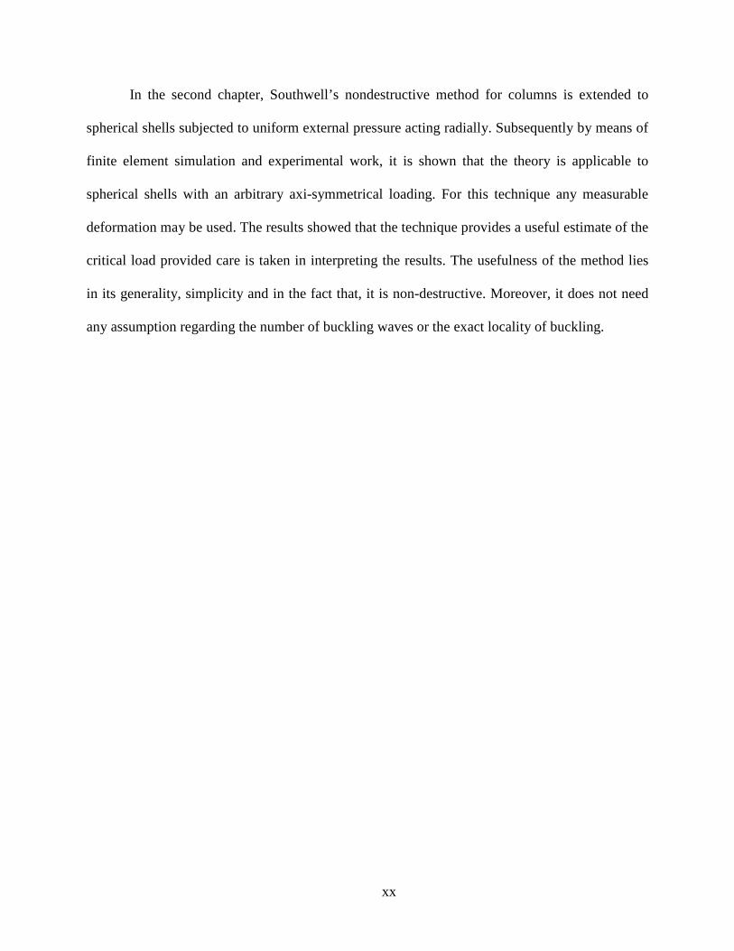
In the second chapter, Southwell’s nondestructive method for columns is extended to
spherical shells subjected to uniform external pressure acting radially. Subsequently by means of
finite element simulation and experimental work, it is shown that the theory is applicable to
spherical shells with an arbitrary axi-symmetrical loading. For this technique any measurable
deformation may be used. The results showed that the technique provides a useful estimate of the
critical load provided care is taken in interpreting the results. The usefulness of the method lies
in its generality, simplicity and in the fact that, it is non-destructive. Moreover, it does not need
any assumption regarding the number of buckling waves or the exact locality of buckling.
xxi
A Review of Literature
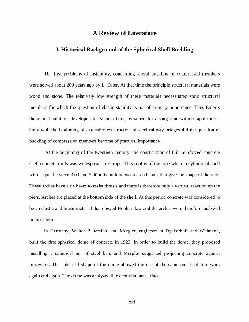
I. Historical Background of the Spherical Shell Buckling
The first problems of instability, concerning lateral buckling of compressed members
were solved about 200 years ago by L. Euler. At that time the principle structural materials were
wood and stone. The relatively low strength of these materials necessitated stout structural
members for which the question of elastic stability is not of primary importance. Thus Euler’s
theoretical solution, developed for slender bars, remained for a long time without application.
Only with the beginning of extensive construction of steel railway bridges did the question of
buckling of compression members become of practical importance.
At the beginning of the twentieth century, the construction of thin reinforced concrete
shell concrete roofs was widespread in Europe. This roof is of the type where a cylindrical shell
with a span between 3.00 and 5.00 m is built between arch beams that give the shape of the roof.
These arches have a tie beam to resist thrusts and there is therefore only a vertical reaction on the
piers. Arches are placed at the bottom side of the shell. At this period concrete was considered to
be an elastic and linear material that obeyed Hooke's law and the arches were therefore analyzed
in these terms.
In Germany, Walter Bauersfeld and Mergler, engineers at Dyckerhoff and Widmann,
built the first spherical dome of concrete in 1922. In order to build the dome, they proposed
installing a spherical net of steel bars and Mergler suggested projecting concrete against
formwork. The spherical shape of the dome allowed the use of the same pieces of formwork
again and again. The dome was analyzed like a continuous surface.

xxii
The construction of the dome at Jena city was made possible by Prof. Spangenberg's report.
Construction began in the winter of 1923-1924. The bars close to the edge started to buckle and
some stabilization bars were needed. In this construction, Bauersfeld analyzed the bending
moment and deformation. In the first dome (Jena, 16.00 m span), not only were the in plane
tension and compression in the plan of the dome taken into account, but bending moments and
deformation were also studied.
The theory of the rigid of dome rotation was published by Föppl, Drang and Zwang. Second
order differential equations were needed to solve the problem. Bauersfeld found an approach
which yielded a solution, in which the Zoelly formula was used to analyze the problem of
buckling, which gives a safety factor of 13.
Bauersfeld asked Dr. Geckeler to undertake some experiments. He did many tests and
found that in the loads close to the Zoelly formula buckling start.
In the autumn of 1933 Torroja began several projects with shell structures. The first
project he undertook was the roof of Algeciras Market. This was a dome of 46.22 m span,
supported by 8 piers. The shell consisted of a spherical concrete construction. The shell was built
using wooden formwork on a scaffold. With this method there was no problem with bars
buckling as had happened to Bauersfeld with the construction of his first dome in Jena.
In 1934 Flügge proposed a value for the critical buckling load of spherical shells. However the
expression was given for a full sphere.
Von Karman and Tsien (1939) showed that the state of stability of some structures,
usually shell like structures, is weak. In other words, a small disturbance might cause them to
snap into a badly deformed configuration. They also attempted to explain the discrepancy
between the classical and excremental buckling pressures for clamped shallow spherical shells

xxiii
under a uniform pressure. After the studies of Von Karman and Tsien (1939), the buckling
problem of spherical shell has been examined both theoretically and experimentally by many
investigators under various types of loading. Tsien (1942) showed that a small disturbance in a
test would cause the shell to jump to a new configuration with large displacements as soon as the
buckling load was exceeded.
Kaplan and Fung (1954) and Simons (1955) studied the buckling behavior of spherical
caps from pressure deflection curve. Their analysis was based on integration of nonlinear finite
deflection equations. Kaplan and Fung (1954) made some experiments for very shallow clamped
spherical caps under a uniform pressure. They compared these results with the ones obtained by
a perturbation solution of the governing nonlinear equations and observed that the agreement
was satisfactory.
Buckling of clamped shallow spherical shells under external pressure has been studied
extensively both experimentally and theoretically. In 1954, Kaplan and Fung performed an
analytical and experimental investigation of clamped shallow spherical shells. Thurston (1961)
obtained a numerical solution for the nonlinear equations for clamped shallow spherical shells
under external pressure and presented the results in the post buckling range not previously
computed. Then he compared the upper buckling and lower post buckling pressures with the
experimental data of Kaplan and Fung (1954).
Huang (1964) worked on the problem of clamped shallow spherical shells for symmetric
and unsymmetric buckling as well. Huang compared his numerical finding with the experimental
results.
Famili and Archer (1965) investigated the buckling behavior of shallow shells by using
the nonlinear equations, considering the asymmetric deformations at the beginning of the

xxiv
buckling to be finite. The nonlinear eigenvalue problem was solved numerically. Their results
were in agreement with those of Huang (1965).
Thurston and Penning (1966) conducted an extensive experimental and analytical
investigation of the buckling of clamped shells with axisymmetric imperfections. They basically
compared the pressure strain and pressure deflection results obtained both experimentally and
theoretically. They found out that the effect of axisymmetric imperfections is not large enough to
give good agreement between theory and experiments for very thin shells.
Hutchinson (1967) studied the initial post buckling behavior of a shallow section of a
spherical shell subjected to external pressure. He found out that imperfection in the shell
geometry have the same severe effect on the buckling strengths of spherical shells as
demonstrated for axially compressed cylindrical shells.
Budiansky (1969) and Weinitschke (1970) also determined the axisymmetric buckling
pressures of shallow spherical shells numerically. There is a good agreement among all the
results obtained.
Fitch (1968) studied the elastic buckling and initial post buckling behavior of clamped
shallow spherical shells under concentrated loading. He determined that bifurcation into an
asymmetric pattern will occur before axisymmetric snap- buckling unless the ratio of the shell
rise to the thickness lies within a narrow range corresponding to moderately thick shells. Fitch
(1970) also investigated the elastic buckling and initial post buckling behavior of clamped
shallow spherical shells under axisymmetric load. He found out that as the area of the loaded
region increase, the buckling behavior changes from asymmetric bifurcation to axisymmetric
snap-through, and then back to asymmetric bifurcation.

xxv
Stricklin and Martinez (1969) studied nonlinear analysis of shells of revolution by the
matrix displacement method. The nonlinear strain energy expression was evaluated using linear
functions for all displacements. Five different procedures were examined for solving the
equations of equilibrium, with Houbolt’s method to be the most suitable. Solutions were
presented for the symmetric and asymmetric buckling of shallow caps under step pressure
loadings and a wide variety of other problems including some highly nonlinear ones. The
difficulty of repeated solutions of a large number of equations has been circumvented by placing
the nonlinear terms on the right hand side of the equations of equilibrium and treating them as
additional loads. The solutions of the governing equations were obtained by iterations and found
to yield accurate results for some practical problems. For highly nonlinear problems, the
equations were solved by the Newton-Raphson procedure, with the coupling between harmonics
being ignored when the nonlinear terms were treated as pseudo loads and taken to the right hand
side of the equations.
Huang (1969) studied the behavior of axisymmetric dynamic snap-through of elastic
clamped shallow spherical shells under impulsive and step loading with infinite duration. It was
observed that the dynamic snap-through buckling was not possible under impulsive loads but it
was achieved under step loading conditions. The results obtained for static uniform pressure and
dynamic loading formed a benchmark for many investigators in the verification of their results.
Axisymmetric and dynamic buckling of spherical caps due to centrally distributed
pressure was studied by Stephens and Fulton (1969). Sanders’ axisymmetric nonlinear elastic
shell theory was approximated by finite difference equations including the Houbolt backward
difference formulation in time. The equations were linearized using an iterative Newton-Raphson
procedure. Axisymmetric buckling loads were given for a spherical cap subjected to a constant

xxvi
static pressure or step pulse of infinite duration distributed axisymmetrically over a portion over
the center of the shell. The influence of the size of the loaded area and of moment and inplane
boundary conditions on both static and dynamic buckling was studied, as well as various
buckling criteria to define dynamic buckling were used.
Grossman et al. (1969) investigated the axisymmetric vibrations of spherical caps with
various edge conditions by carrying out a consistent sequence of approximations with respect to
space and time. Numerical results were obtained for both free and forced oscillations involving
finite deflections. The effect of curvature was examined with particular emphasis on the
transition from a flat plate to a curved shell. In such a transition, the nonlinearity of the
hardening type gradually reversed into one of softening.
Tillman (1970) presented the results of a theoretical and experimental investigation into
elastic buckling of clamped shallow spherical shells under a uniform pressure, focusing mainly
on low values of the geometric parameter, for which the symmetrical and first two asymmetrical
deformations are valid.
Archer (1981) studied the behavior of shallow spherical shells subjected to dynamic loads
of sufficient magnitude to result in finite nonlinear axisymmetric deformations. Marguerre’s
equations for the small finite deflections of shallow shells with the inclusion of inertia terms
were taken as the governing equations. Results for the quasi statically loaded shell before and
after snap through and snap back were studied and compared with known results. The dynamic
response of the shell to rectangular pulse loading and buckling loads were obtained.
Dynamic buckling of orthotropic shallow spherical shells by Ganapathi and Varadan
(1982) and axisymmetric static and dynamic buckling of orthotropic shallow spherical cap with
circular hole by Dumir (1983) were investigated.

xxvii
Geometric nonlinear 3D dynamic analysis of shells based on a total Largrangian
formulation and the direct time integration of the equation of motion was derived by Wouters
(1982).
Dumir et al. (1984) investigated axisymmetric buckling of orthotropic shallow spherical
cap with circular hole. Analysis has been carried out for uniformly distributed load and a ring
load at the hole.
Zheng and Zhou (1989) developed semi-analytical computer method to solve a set of
geometrically nonlinear equations of plates and shells. By this method, analytical solutions such
as exact expansion in series, perturbations and iterations of the equations can be obtained.
Hsiao and Chen (1989) used a degenerated isoparametric shell element for the nonlinear
analysis of shell structures. Six types of rotation variables and rotation strategies were employed
to describe the rotation of the shell normal. In particular, a finite rotation method was proposed
and tested. Both the rotation variations between two successive increments and the rotation
corrections between two successive iterations were used as the incremental rotation (rotation
variables) to update the orientation of the shell normal.
Chan and Chung (1989) used higher order finite elements for the geometrically nonlinear
analysis of shallow shells. Based on K. Marguerre’s shell theory, a family of higher order finite
elements was developed. A step iteration Newton-Raphson scheme was adopted in solving the
final system of nonlinear equations.
Bhimaraddi and Moss (1989) developed a shear deformable finite element for the
analysis of general shells of revolution.
Xie, Chen and Ho (1990) studied the nonlinear axisymmetric behavior of truncated
shallow spherical shells under transverse loading. Load-deflection relation were obtained

xxviii
through iteration and numerical integration. Shells subjected to uniform pressure and combined
uniform pressure and concentrated ring loading were investigated.
Eller (1990) derived finite element procedures for the stability analysis of nonlinear
periodically excited shell structures. Starting from a geometrically nonlinear shell theory and
applying Ljapunow’s first method as well as Floquet’s theory, a numerical stability criterion was
deduced.
Luo et al. (1991) investigated the influence of pre buckling deformations and stresses on
the buckling of the spherical shell. They obtained from Von Karman's large deflection equation
of the plate and by assuming that a plate has an initial deflection in the form of a spherical cap,
the equilibrium equations of a spherical cap subjected to hydrostatic pressure were written.
Chang (1991) developed a non-linear shear-deformation theory for the axisymmetric
deformations of a shallow spherical cap comprising laminated curved-orthotropic layers. He
expressed the governing equations in terms of the transverse displacement, stress function and
rotation. Numerical results on the buckling and post-buckling behavior of spherical caps under
uniformly-distributed loads were presented for various boundary conditions, cap rises, base
radius-to-thickness ratios, numbers of layers and material properties.
Delpak and peshkm (1991) developed a variational approach to the geometrically
nonlinear analysis of asymmetrically loaded shells revolution. The formulation was based on
taking the second variation of the total potential energy equation. The analysis commenced by
taking the first and second variation of the total potential energy of the elastic system by ensuring
that load increments were applied infinitely slowly. After separating the load and the stiffness
terms and factorizing the nodal variables, a distinct demarcation in the contribution of linear and
xxix
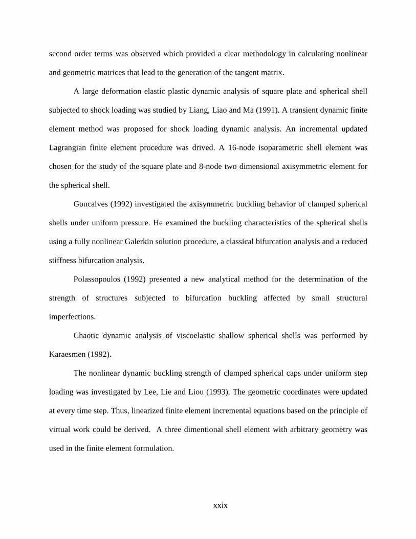
second order terms was observed which provided a clear methodology in calculating nonlinear
and geometric matrices that lead to the generation of the tangent matrix.
A large deformation elastic plastic dynamic analysis of square plate and spherical shell
subjected to shock loading was studied by Liang, Liao and Ma (1991). A transient dynamic finite
element method was proposed for shock loading dynamic analysis. An incremental updated
Lagrangian finite element procedure was drived. A 16-node isoparametric shell element was
chosen for the study of the square plate and 8-node two dimensional axisymmetric element for
the spherical shell.
Goncalves (1992) investigated the axisymmetric buckling behavior of clamped spherical
shells under uniform pressure. He examined the buckling characteristics of the spherical shells
using a fully nonlinear Galerkin solution procedure, a classical bifurcation analysis and a reduced
stiffness bifurcation analysis.
Polassopoulos (1992) presented a new analytical method for the determination of the
strength of structures subjected to bifurcation buckling affected by small structural
imperfections.
Chaotic dynamic analysis of viscoelastic shallow spherical shells was performed by
Karaesmen (1992).
The nonlinear dynamic buckling strength of clamped spherical caps under uniform step
loading was investigated by Lee, Lie and Liou (1993). The geometric coordinates were updated
at every time step. Thus, linearized finite element incremental equations based on the principle of
virtual work could be derived. A three dimentional shell element with arbitrary geometry was
used in the finite element formulation.

xxx
Terndrup et al. (1995) studied the buckling behavior of imperfect spherical shells
subjected to different loading conditions. They analyzed the bifurcation and initial post-buckling
behaviour of highly imperfection-sensitive large spherical .shells, such as cargo tanks for ship
transportation of liquefied natural gas and large spherical containment shells for nuclear power
plants.
Zhang (1999) studied the torsional buckling of spherical shells under circumferential
shear loads. He used Galerkin variational method, for studying the general stability of the hinged
spherical shells with the circumferential shear loads.
Uchiyama et al. (2003) studied nonlinear buckling of elastic imperfect shallow spherical
shells by mixed finite elements. They used nine-node-shell element and mixed formulation for
stress resultant vectors then they compared finite element results with fifty-two experiments on
the elastic buckling of clamped thin-walled shallow spherical shells under external pressure.
Grünitz (2003) examined the buckling strength of clamped and hinged spherical caps
under uniform pressure with a circumferential weld depression by using the finite element
method. The results obtained show a significant decrease in the buckling strength due to these
imperfections depending on the location of the weld.
Dumir et al. (2005) presented axisymmetric buckling analysis for moderately thick laminated
shallow annular spherical cap under transverse load. In their study, buckling was considered
under uniformly distributed transverse load, applied statically. Annular spherical caps have been
analyzed for clamped and simple supports with movable and immovable in-plane edge
conditions and typical numerical loads and have been compared with the classical lamination
theory.
xxxi
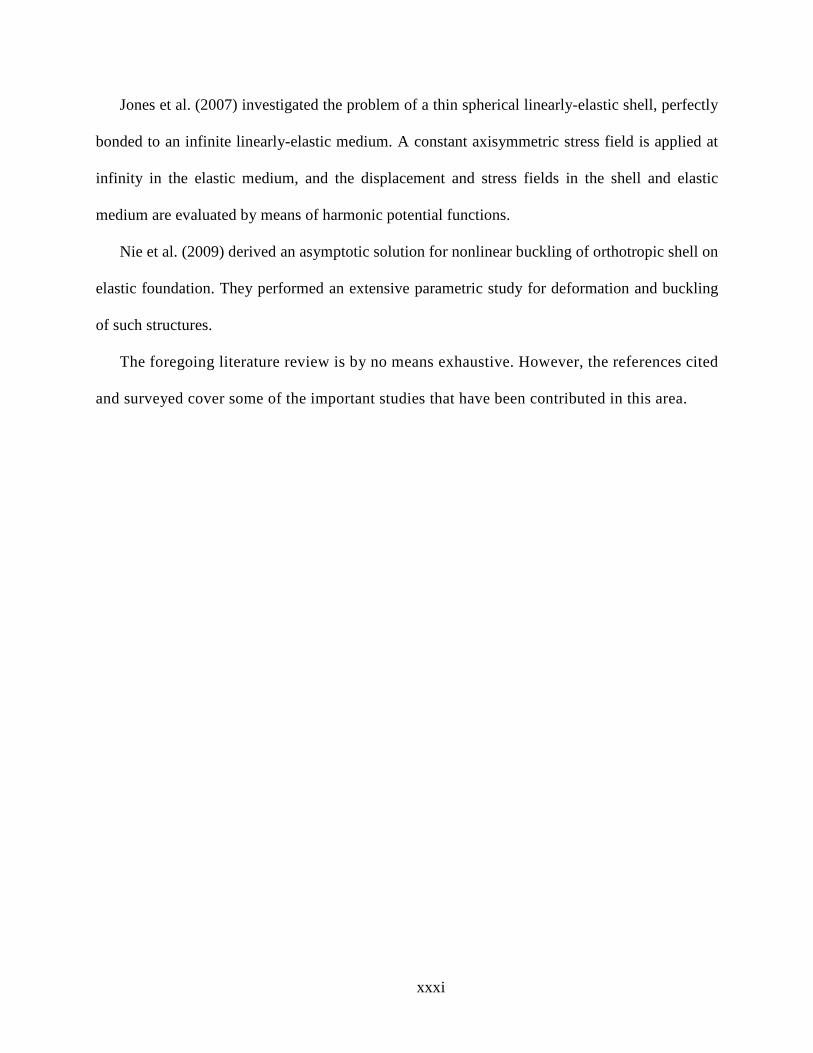
Jones et al. (2007) investigated the problem of a thin spherical linearly-elastic shell, perfectly
bonded to an infinite linearly-elastic medium. A constant axisymmetric stress field is applied at
infinity in the elastic medium, and the displacement and stress fields in the shell and elastic
medium are evaluated by means of harmonic potential functions.
Nie et al. (2009) derived an asymptotic solution for nonlinear buckling of orthotropic shell on
elastic foundation. They performed an extensive parametric study for deformation and buckling
of such structures.
The foregoing literature review is by no means exhaustive. However, the references cited
and surveyed cover some of the important studies that have been contributed in this area.

xxxii
II. A Brief History of Yield Line Theory
As early as 1922, the Russian, A. Ingerslev presented a paper to the institution of
Structural Engineers in London on the collapse modes of rectangular slabs. Later on yield Line
theory as it is known today was pioneered in the 1940s by the Danish engineer and researcher
KW Johansen.
Authors such as R. H. Wood, L. L. Jones, A. Sawczuk and T. Jaeger, R. Park, K. O.
Kemp, C.T. Morley, M. Kwiecinski and many others, consolidated and extended Johansen’s
original work so that now the validity of the theory is well established. In the 1960s, 1970s, and
1980s a significant amount of theoretical work on the application of yield line theory was carried
out around the world and was widely reported. To support this method, extensive testing was
undertaken to prove the validity of the theory. Excellent agreement was obtained between the
theoretical and experimental yield line patterns and the ultimate loads. The differences between
the theory and tests were small and mainly on the conservative side.

xxxiii
III. Historical Background of the Southwell Method
Sir Richard Vynne Southwell (1888– 1970) was a British mathematician who specialized
in applied mechanics as an engineering science academic. Richard Southwell was educated at the
University of Cambridge, where in 1912 he achieved first class degree results in both the
mathematical and mechanical science tripos. In 1914, he became a Fellow of Trinity College,
Cambridge, and a lecturer in Mechanical Sciences. Southwell was in the Royal Naval Air
Service during World War I. After World War I, he was head of the Aerodynamics and
Structures Divisions at the Royal Aircraft Establishment, Farnborough. In 1920, he moved to the
National Physical Laboratory. He then returned to Trinity College in 1925 as Fellow and
Mathematics Lecturer. Next, in 1929, he moved to Oxford University as Professor of
Engineering Science and Fellow of Brasenose College. There, he developed a research group,
including Derman Christopherson, with whom he worked on his relaxation method. He became a
member of a number of UK governmental technical committees, including the Air Ministry, at
the time when the R100 and R101 airships were being conceived.
Southwell was rector at Imperial College, London from 1942 until his retirement in 1948.
He continued his research at Imperial College. He was also involved in the opening of a new
student residence, Selkirk Hall.
As a scientist, in 1932, Southwell presented his analysis for the special case of a pin
ended strut of constant flexural rigidity of EI . Southwell method for determining the minimum
buckling load is a nondestructive test for pined-end, initially imperfects struts. Southwell showed
that the load deflection curve of such a member is a hyperbolic in the neighborhood of the
smallest critical load, while the asymptote is a horizontal line, crPP = . By suitable

xxxiv
transformation of variables this hyperbolic portion of load deflection curve may be converted
into a straight line for which the inverted slope is the minimum critical load.
1
CHAPTER 1 - Plastic Buckling of Hemispherical Shell Subjected
to Concentrated Load at the Apex
1.1 Introduction and Purpose of this Chapter
Due to the increasing use of shell type structures in space vehicles, submarines, buildings
and storage tanks, interest in the stability of shells has accordingly increased by researchers and
practicing engineers. Because a hemispherical shell is able to resist higher pure internal pressure
loading than any other geometrical vessel with the same wall thickness and radius, the
hemispherical shell is one of the important structural elements in engineering applications. It is
also a major component of pressure vessel construction. In practice, most pressure vessels are
subjected to external loading due to hydrostatic pressure, or external impact in addition to
internal pressure. Consequently, they should be designed to resist the worst combination of
loading without failure. The load transmitted by a cylindrical rigid actuator applied at the summit
of the sphere is considered a common external load. Thus, it is important to study its effect on
the initial buckling and plastic buckling propagation of this type of shells. This study presents
the analytical, numerical, and experimental results of moderately thick hemispherical metal
shells into the plastic buckling range illustrating the importance of geometry changes on the
buckling load. The hemispherical shell is rigidly supported around the base circumference
against vertical and horizontal translation and the load is vertically applied by a rigid
cylindrical boss at the apex. Kinematic stages of initial buckling and subsequent propagation of
plastic deformation for rigid-perfectly plastic shells are formulated on the basis of Drucker-
Shield's limited interaction yield condition. The effect of the radius of the boss, used to
apply the loading, on the initial and subsequent collapse load is studied. In the numerical

2
model, the material is assumed to be isotropic and linear elastic perfectly plastic without strain
hardening obeying the Tresca or Von Mises yield criterion. Both axisymmmetric and 3D models
are implemented in the numerical work to verify the absence of non-symmetric deformation
modes in the case of moderately thick shells. In the end, the results of the analytical solution are
compared and verified with the numerical results using ABAQUS software and experimental
findings. Good agreement is observed between the load-deflection curves obtained using the
three different approaches. The preparations to conduct experimental verifications are also
shown in Fig. 1.1.
Figure 1. 1: Sample construction procedure for the experimental study

3
1.2 Preliminary Considerations
This study is focused on the following physical phenomenon. A hemispherical shell is
compressed by a concentrated load at the summit. At the load below a certain critical value,
called the initial buckling load, the shell remains spherical or unbuckled but when the increasing
applied load reaches the critical initial buckling value, the shell snaps into a non-spherical
buckled state which is characterized by a round dimple around the apex of the hemispherical
shell. Therefore, it creates a deformation state which extends or propagates over the surface of
the shell leaving undetermined the amplitude of deformation at various levels of load (Fig. 1.2).
Figure 1. 2: Geometry and post buckling of hemispherical shells subjected to a concentrated load
4
1.3 Analytical Formulation
1.3.1. Kinematics Assumptions
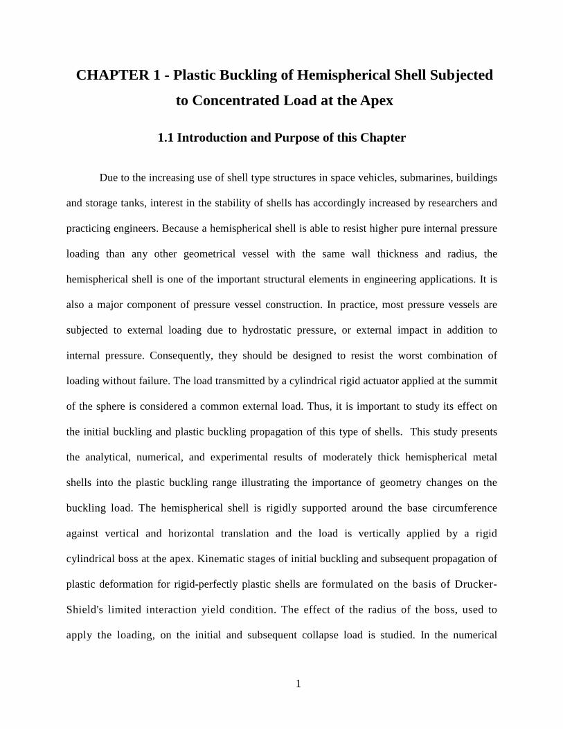
The behavior of a moderately thick metal hemispherical shell under a concentrated load
at the summit may be analyzed as follows:
a) The perfectly-rigid state culminating at the attainment of the initial collapse load0P .
For a concentrated load acting on a hemispherical shell the initial collapse takes place only
in a vanishingly small region of the shell, Fig. 1.3. The collapse load 0P depends on the
plastic moment 0M of the shell material. If a rigid cylindrical boss is used for loading purposes, the
size of this boss influences the region of collapse and hence the collapse load0P .
Figure 1. 3: Initial buckling under concentrated load

5
b) Deformation under the collapse load0P .
At the load 0P , the shell snaps to reverse its curvature and continues to deform under the
same load, resulting in the formation of a dimple. The dimple is taken to be conical in shape and
the apex of the cone is the point where the load is acting. This assumption is not at variance with
the observed behavior. The extent of the dimple depends again on the plastic moment 0M of the
shell material and on the radius of the loading boss or actuator. A section of the shell through a
meridional plane, immediately after the deformation under the initial collapse load 0P , is
shown in Fig.1.4.
The outer undeformed portion of the shell (of radius R and constant thickness0t ) and
the conical dimple are connected by an annular zone to which the cone is tangent, and which
shares a common tangent with the undeformed part of the shell. Both the conical dimple,
and the annular zone which looks in section like a knuckle of radius ρ symmetrical about
the axis of revolution, are plastic.
Figure 1. 4: Post buckling deformation at initial collapse load 0
P
6
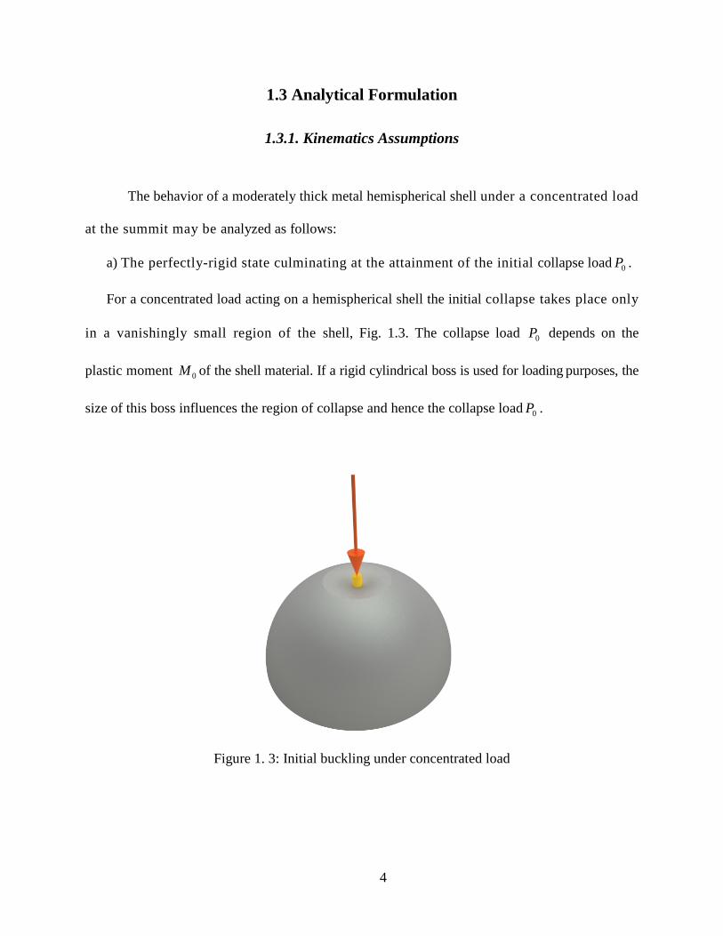
c) Propagation of the annular zone.
This is the third stage of deformation. It takes place only after the deformation under the
constant load 0P is complete. The dimple extends outward with an axisymmetric deformation
under an increasing load P to render a greater portion of the shell plastic Fig.1.5. The
deformation involves a conical shape and an annular zone.
Figure 1. 5: Plastic buckling deformation extends outward under an increasing load P
d) Degeneration of the shape of deformation.
After the annular zone (which is circular in plan) has propagated to an extent depending
for a given material on the 0/ tR ratio, the axisymmetric deformation described above
begins to change. The annular zone becomes triangular and then polygonal in plan. A new
mechanism which involves the folding of the shell material about the edges of a pyramid-like
surface takes over and replaces the conical part of the deformation. This phenomenon could be
associated with some sort of a secondary instability. This stage of deformation will not be
addressed in part of this study, because it is unlikely to take place in moderately thick shells.
7
1.3. 2. The Initial Collapse Load and Reversal of Curvature
Shells are commonly subjected to transverse loads, i.e. loads that act in the direction
perpendicular to the surface of the shell. Such shells may fail locally by so called fan mechanism,
with positive yield lines radiating from the point load. Consequently, at sufficiently high load,
the shells may experience extensive plastic deformation locally and eventually lose all its
structural function and changes its curvature direction this phenomenon known as local plastic
collapse.
Unlike elastic analysis, exact solutions for the plastic collapse load are not available in
most cases. Even for the idealized rigid perfectly plastic constitutive relation, the collapse load
can only be approximated over a range of values. The technique used to define the boundary of
the collapse load is known as limit load and the theorem associated with it known as limit
analysis.
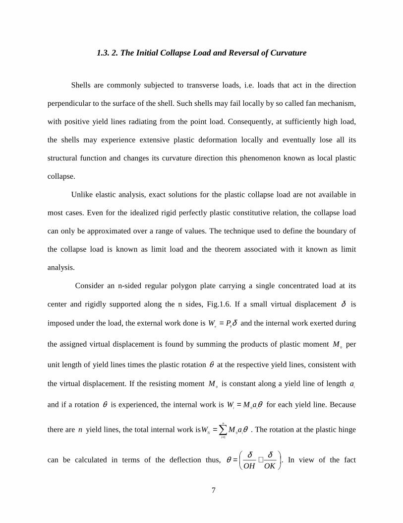
Consider an n-sided regular polygon plate carrying a single concentrated load at its
center and rigidly supported along the n sides, Fig.1.6. If a small virtual displacement δ is
imposed under the load, the external work done is δ0
PWe
= and the internal work exerted during
the assigned virtual displacement is found by summing the products of plastic moment 0
M per
unit length of yield lines times the plastic rotation θ at the respective yield lines, consistent with
the virtual displacement. If the resisting moment 0
M is constant along a yield line of length i
a
and if a rotation θ is experienced, the internal work is θii
aMW0
= for each yield line. Because
there are n yield lines, the total internal work is ∑=
=n
iiTi
aMW1
0θ . The rotation at the plastic hinge
can be calculated in terms of the deflection thus,
+=OKOH
δδθ . In view of the fact
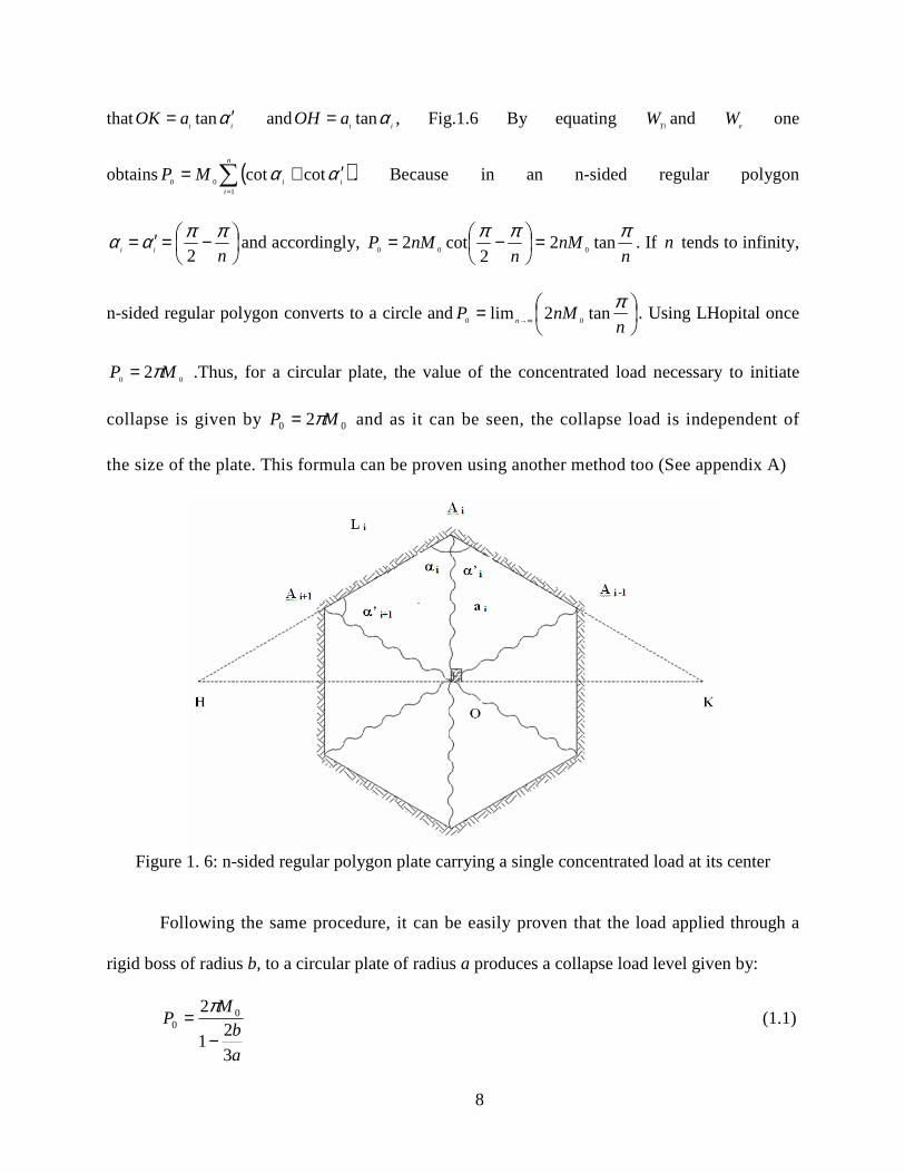
8
thatii
aOK α ′= tan andii
aOH αtan= , Fig.1.6 By equating Ti
W and e
W one
obtains ( )∑=
′+=n
iii
MP1
00cotcot αα . Because in an n-sided regular polygon
−=′=nii
ππαα2
and accordingly, n
nMn
nMPπππ
tan22
cot2000
=
−= . If n tends to infinity,
n-sided regular polygon converts to a circle and
= ∞→ nnMP
n
πtan2lim
00. Using LHopital once
002 MP π= .Thus, for a circular plate, the value of the concentrated load necessary to initiate
collapse is given by 00 2 MP π= and as it can be seen, the collapse load is independent of
the size of the plate. This formula can be proven using another method too (See appendix A)
Figure 1. 6: n-sided regular polygon plate carrying a single concentrated load at its center
Following the same procedure, it can be easily proven that the load applied through a
rigid boss of radius b, to a circular plate of radius a produces a collapse load level given by:
a
bM
P
3
21
2 00
−=
π (1.1)

9
The region of a hemisphere subjected to downward concentrated load at the apex that
initially collapses with a reversal of curvature is quite small and can be easily considered to be
a very shallow spherical cap. If the boss size is ignored, 02 Mπ is known to be the exact
collapse load for any circular plate and therefore it can serve as a lower bound on the initial
collapse load of a shallow spherical cap. The initial collapse load of a hemispherical shell under
a concentrated load should thus approach the value 02 Mπ because the local nature of the
collapse may mean that the collapse load is less dependent on the shell curvature. When the shell
is loaded by means of a finite rigid boss of radius b, the collapse load 0P has a value which is
observed to be greater than 02 Mπ while it is dependent on the size. As mentioned earlier, this is
also true of a plate loaded with a boss, and so the same modification of the collapse load
formula referred to above can be made. The difference is that while the flat plate radius a is
known, the dimple planner radius at initial collapse in the case of a hemispherical shell is not
readily available but has to be calculated. The value of this dimple radius for the shell is
found by equating the initial collapse load 0P with the load predicted by the mechanism of
dimple propagation at the start of the third stage of deformation, as shown below. The initial
collapse and subsequent deformation mechanism can be seen in Fig. 1.7.
The shell initially collapses at a load value of 0P which is equal to or greater than 02 Mπ
to an extent depending on the boss radiusb . A portion of the shell shown as a dotted line at
its initial position as part of a hemisphere of radius R takes up the buckled position shown
by the bold line, comprising a cone and an annular zone, Fig.1.7 The extent of the
deformation is measured by 0θ the meridional angle corresponding to the boundary of the

10
plastic region. During this deformation, the load 0P remains constant. It is between these
initial and final positions that the toroidal annular zone with the knuckle radius ρ and the cone
come into being. It is only after this stage is complete that the third stage of deformation with a
different type of mechanism takes over. This comprises the propagation of the dimple and the
outward movement of the annular zone.
Figure 1. 7: Profile of deformation during initial buckling and post buckling behavior

11
In the ideal case of a concentrated load acting at the shell apex, it is natural to
expect that the second step of deformation should begin almost immediately after the shell load
reaches the value0
2 Mπ . The following geometrical relations in which the boss will not play a
significant part can be derived for the initial collapse using the incompressibility condition, and
assuming no difference between the thickness of the shell in the dimple region before and after
collapse:
The surface area of the spherical cap which reverses curvature is:
Surface Area initial= )cos1(2 02 θπ −R . (1.2)
This must be equated to the sum of the surface areas of the cone and the annular zone,
which are equal to:
Surface Area Buckled=Surface area of annular part + Surface area on conical part=
( ) ( )0
0
22
00 cos
sin22.sin2
θθρπρθθρπ −
+−R
R (1.3)
Equating eqs. (1.2) and (1.3) then simplifying, the following equation is obtained:
( ) ( )0
0
22
000 cos
sin/21
2
1sin/1
2cos1
θθρθθρρθ RR
R−+−=− (1.4)
As 0θ is small, 24/2/cos1 4
0
2
00θθθ −=− , and 6/sin 3
000θθθ −= . Neglecting the second
terms on the right hand side of the cosine and sine series expansions and ignoring the fourth
power of 0θ would make equation (1.4) trivially satisfied. Substituting these values into equation
(1.4) and neglecting powers of 0θ higher than the fourth, the equation reduces to:
016/32
2
4
0=
+−RR
ρρθ (1 .5 )

12
For any non-zero value of0θ , the solution gives 25.0/ =Rρ and/ or 0.75. For the larger
value of ρρ 2,75.0/ −= RR becomes negative, which means that the conical part of the dimple
cannot exist. Thus the relevant value of ρ is 4/R . Although 0θ has a small value, it can be
assumed that ρ is equal to 4/R throughout the subsequent deformation for which θ is
greater than0θ roughly until 0296.571 =≅ radθ since all assumptions are satisfied.
1.3.3. Propagation of the Dimple
During the formation of the initial dimple, the deformation is small and the buckling
happens under a constant load0P . As the deflection increases, the effect of geometry change
starts to become significant and the load increases with continuing deformation. When the
non-plastic material surrounding the deforming region cannot support a load higher than 0P , the
plastic region must grow in size with increasing load. It is assumed here that the deforming
surface maintains a geometrical similarity during the propagation of the dimple as evidenced by
the the numerical results. The deformation stage being identified by a single parameterθ , which
is the angular position of the surface at the boundary of the plastic region (Fig.1.7). It is
assumed that the radius of curvature of the toroidal knuckle remains constant while its
crown moves away from the axis of revolution by continuous rotation and translation of the rigid
material entering into the plastic region.
The middle surface of the deforming shell forms a surface of revolution and the state of
stress is completely specified by the direct forces, resultant moments and transverse shear. If φN
and βN denote the meridional and circumferential forces per unit length, φM and βM the cor-

13
responding bending moments, and Q the transverse shear force (Fig. 1.8), the meridional
equations of equilibrium for a shell of revolution can be written as
0cos)( 1 =−−∂∂
rQNrrN φφ βφ (1.6)
0cos)( 11 =−−∂∂
QrrMrrM φφ βφ (1.7)
where r is the distance of the element from the axis of revolution and 1
r its mean
meridional radius of curvature, which is equal to ρ at the annular zone.
Figure 1. 8: Equilibrium of an axisymmetric shell element

14
In our assumed deformation model, the annular zone has a constant radius of curvatureρ ,
It is easily visualized that φN changes sign from positive (tension) to negative (compression) as
we move from the inner to the outer part of the toroidal knuckle.
φN at the boundary of the cone annular zone is tension and at the boundary of the
annular zone- undeformed shell is compression to resist the downward P such that∑ = 0yF . In
other words, under increasing load the shell material from the outer undeformed region is pushed
into the annular zone and material from the annular zone is pulled into the conical dimple.
Thus φN may be assumed to vanish at the crown of the toroid. Considering the outer part of the
knuckle defined by θφ ≤≤0 and noting that φN is compressive in this region, it is evident
that βN should also be compressive. This is due to the fact that compressive φN causes
expansion in the hoop direction while the rigid shell restraints the knuckle from expansion thus
inducing compressive stress:
,0tN σβ −= (1.8)
where 0σ is the (constant) yield stress of the material and t is the current thickness. The
first equation of equilibrium, equation (1.6), therefore reduces to
( ) rQtNr +−=∂∂ φρσφ φ cos
0 (1.9)
This equation must be supplemented with the equation of vertical equilibrium, namely
( ) PQNr −=+ φφπ φ cossin2 (1.10)
where P is the total vertical downward load at the conical apex. Eliminating Q
between (1.9) and (1.10),

15
( ) φπ
ρσφφ φ
20 sec
2sec
PtNr −−=
∂∂
(1.11)
Assuming that the thickness variation may be neglected in the equilibrium equations
and noting that 0tt = (the initial thickness) at θφ = , equation (1.11) can be integrated to
obtain
,sin2
cos00
+−= φπ
φφρσφ
PtNr (1.12)
where 0=φN at 0=φ is used as a boundary condition.
Considering the moment equation of equilibrium, it is observed that the second term of
equation (1.7) is of the order of rt / times that of the last term, as proven by Drucker & Shield
(1959), and hence the second term may be neglected when the region of interest is not close
to the axis of revolution. Equation (1.7) then reduces to
( ) QrMr ρφ φ =
∂∂
(1.13)
From eqs. (1.10) and (1.12),
φπ
φφσρ cos2
sin00
PtQr −= (1.14)
and eq. (1.13) becomes
( )
−=
∂∂ φ
πφφσρρ
φ φ cos2
sin00
PtMr (1.15)
Since the crown of the toroidal knuckle suffers the most severe bending, it is
natural to assume that φM at the crown is equal to the yield moment 0M . It may also be

16
assumed that at the boundary of the rigid region, φM attains the value of the yield
moment. Neglecting again the thickness variation, the boundary conditions can be written
0MM −=φ at 0=φ and θφ = . Integration of eq. (1.15) between the limits of 0 and θ gives:
( ) CP
t
CP
dttdP
dtrM
+−−=
+−+−=−= ∫∫∫
φπ
ρφφφσρ
φπ
ρφφσρσφρφφφρπ
φφφσρφ
sin2
cossin
sin2
coscoscos2
sin
00
2
00
2
00
2
00
2
θρθφ φ sinsin0000
MMRCMM +−=→−=→=
0MM −=→= φθφ
( ) θρθθπ
ρθθθσρθ sinsinsin2
cossinsin 00002
0 MMRP
tMR +−−−=−
This will then lead to:
( ) θπ
θθθρσθ sin2
cossinsin 000
PtM −−=− (1.16)
Inserting the values 4
200
0
tM
σ= and ,
4
R=ρ equation (1.16) reduces to
−+=θ
θπ tan
1/12 0
0
tRM
P (1.17)
This formula directly relates the downward vertical load to the angular position of the
dimple denoted by 0θθ ≥ . It is independent of the size of the boss, provided the diameter of
the boss is small in comparison with the diameter of the shell. For a truly concentrated load 0θ is
vanishingly small and the solution reduces to the well known result 00 2 MP π= .
17
1.3.4. Solution of the Complete Problem
If the shell is loaded by a concentrated load at the apex, the formula (1.17) provides the
complete load- deformation characteristic of the shell. However, a fully concentrated load is only
a mathematical convenience which cannot be realized in practice. In fact the initial collapse load
is very sensitive to the size of the boss and a small boss can considerably increase the collapse load
from the value 00 2 MP π= . It is therefore essential to include the boss size in developing a realistic
theory.
The initial angle for the propagating dimple 0θ is also a measure of the plastic region
corresponding to the initial collapse. Assuming that this small portion of the shell behaves
like a plate during collapse even when the load is applied by a finite boss in the form of a rigid
punch of a small base radius b, equation (1.1) can be rewritten as:
0
0
0
32
1
12
θπ
R
bM
P
−= (1.18)
Since the load corresponding to the beginning of the dimple propagation is also 0P , eq.
(1.17) gives
−+=
0
0
00
0
tan11
2 θθ
π t
R
M
P (1.19)
Since 0θ is small, therefore;
+++
−=
− ....
15
2
3
1tan
1 5
0
3
0
0
0
0
0
θθθ
θθ
θ

18
If the power greater than three is neglected so,
3311
tan1
31
31
13
1
11
tan1
20
20
0
0
0
0
00
0
2
2
2
θθθ
θθ
θ
θθθ
=
−−=−⇒
−=+
+−=
−
Thus,
31
2
2
0
00
0θ
π t
R
M
P+= (1.20)
Equations (1.18) and (1.20) furnish the following equation for 0θ :
,2
32 0
020 R
t
b
R =
−θθ (1.21)
which can be solved numerically for each particular case. An immediate conclusion
from (1.21) is that 0θ is always greater than Rb / . It is easily seen from the geometry in
Fig.1.7 that the punch penetration corresponding to the position of the dimple given by θ is
θθρθ tansin)2()cos1( −+−= RRh (1.22)
and
( )( )θθ sec3cos12
1 +−=R
h (1.23)
by using the result 4/R=ρ .
Eqs. (1.17) and (1.23) give the load-deflection relationship parametrically through θ
when 0θθ ≥ .

19
When 100ptR , this solution is found to correct for large amplitudes of deflection, however
for 100ftR the deformation follows the same axisymmetric pattern in the beginning. Then, the
annular zone degenerates into various n-sided polygon deformation modes and bifurcation in
deformation pattern is observed. In order to determine the bifurcation point during deformation,
assume the deformed part behaves similar to a clamped circular plate of radiuscwith large
deformation before bifurcation point (Fig. 1.9). For thin circular clamped plate the radial and
tangential moments are (see Appendix B):
Figure 1. 9: Deformed part of hemispherical shell shape before the secondary bifurcation point
Figure 1. 10: Effect of axial force on plastic moment capacity
20
( )
−+= 1ln14 r
cPM r υ
π (1.24)
( )
−+= υυπ r
cPM t ln1
4 (1.25)
In the bifurcation point θθρθ ρsin4
3sinsin 4 RcRcR
= →−= =
Assuming that at the bifurcation point, tM reaches to the plastic moment
at θθρ sin2sin Rcr =−= (as evidenced by the numerical and experimental findings). By
combining equations (1.17) and (1.25) and inserting the value
−+=θ
θπtan
1/12 00 tRMP it
can be written:
( ) →
−+
−+== υ
θ
θυ
πθ
θπ
sin2
sin43
ln14
tan1/12 00
R
RtRM
MM plastict
Because of the membrane effect, shell plastic moment is not 4
20
0
tM
σ= anymore and it will be
almost equal to4
ˆ20
0
tMM p
σ−≈ . In this equation,
0sin2ˆ
θσπυ
r
Pt = and consequently:
( )[ ] →−+
−+= υυ
θθ
5.1ln12
tan1/1 00 tRM
M P
Hence:
( )[ ]υυθ
θσσ
−+
−+=− 5.1ln1
2
tan1/1
4
4
ˆ 0
200
20
0
tRt
tM (1.26)

21
In the last stage of deformation, hemispherical shell will be punched under the point load.
Subsequently; the ultimate bearing capacity is roughly equal to:
000
22 σπ t
tbPU
+≈ (1.27)

22
1.4. Nonlinear Finite Element Analysis (FEA)
1.4.1 Elements and Modeling
Finite element analysis (FEA) is capable of modeling elastic-perfectly plastic material
behavior with nonlinear geometry where the analysis is based on the initial geometrical shape.
This should give a limit load and load-deformation response almost equal to the rigid-plastic
limit load and overall response since the elastic deformations are negligible compared to the
plastic deformations. This makes it possible to compare the results using the finite element
method with those of the analytical solution. All FEA for this investigation was performed using
the general purpose program ABAQUS Version 6.7. The boss used to load the spherical shell
was modeled as a rigid element. Both eight node axisymmetric rectangular and six node
triangular shell elements were used to model the hemispherical shell Figs.1.11-1.13. In the
present numerical analyses, the hybrid element was chosen for all finite element models in order
to avoid the problem of mesh locking and to get correct element stiffness and accurate results.
The shell is pinned at the base and the material behavior after yielding is assumed to obey the
Tresca or Von Mises yield criterion.
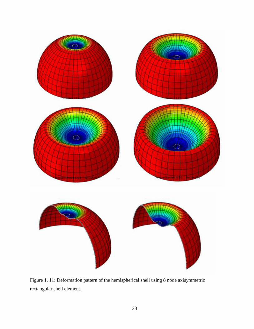
23
Figure 1. 11: Deformation pattern of the hemispherical shell using 8 node axisymmetric
rectangular shell element.
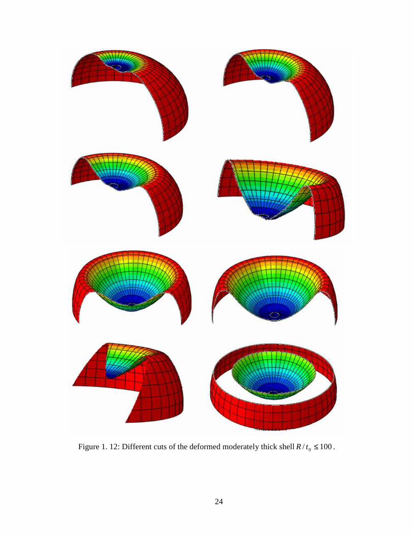
24
Figure 1. 12: Different cuts of the deformed moderately thick shell 100/ 0 ≤tR .

25
Figure 1. 13: Deformation pattern of the moderately thick shell 100/ 0 ≤tR using six node
triangular shell element.
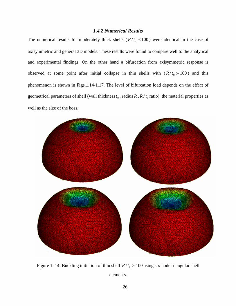
26
1.4.2 Numerical Results
The numerical results for moderately thick shells ( 100/0ptR ) were identical in the case of
axisymmetric and general 3D models. These results were found to compare well to the analytical
and experimental findings. On the other hand a bifurcation from axisymmetric response is
observed at some point after initial collapse in thin shells with ( 100/ 0 ftR ) and this
phenomenon is shown in Figs.1.14-1.17. The level of bifurcation load depends on the effect of
geometrical parameters of shell (wall thickness0t , radiusR , 0/ tR ratio), the material properties as
well as the size of the boss.
Figure 1. 14: Buckling initiation of thin shell 100/ 0 ftR using six node triangular shell
elements.

27
Figure 1. 15: Subsequent deformation of thin shell 100/ 0 ftR showing the secondary
bifurcation phenomenon.

28
Figure 1. 16: Different cuts of the deformed thin shell 100/ 0 ftR

29
Figure 1. 17: Deformation pattern of the thin shell 100/ 0 ftR showing the secondary
bifurcation phenomenon.

30
1.5. Experimental Program
1.5.1 Parameters and test setup
Different samples with various 0
/ tR ratios were designed, manufactured, and tested,
Figs. 1.18. These were made out of Bronze ( GPaE 120= and MPaFy 110= ), stainless steel
( GPaE 210= and MPaFy 315= ), and copper ( GPaE 116= and MPaFy 132= ). The radius of
the shells was mmR 50= and mmR 75= respectively. The thickness of the shells were
mmt 3.00
= and mmt 10
= . These parameters yield 0/ tR ratio of 250 for Bronze, 166 for Stainless
Steel, and 75 for Copper alloy. During testing, these shells were subjected to concentrated loads
at the apex by means of rigid flat-based circular rods of three different boss sizes, namely
mmb 5.0,25.0,125.0= (Fig.1.19).

31
Figure 1. 18: Different hemispherical shell samples were made for experimental study
Figure 1. 19: Three different boss size used for loading ( )mmb 0.5,5.2,25.1=

32
The hemispherical shells were rigidly supported against translation around the bottom
circumference by using grooved base plate as shown in Fig.1. 20.
Figure 1. 20: Grooved base plate as a support for two sizes of hemispherical shells
The load-deflection curves for the shells were recorded on a Riehle Universal testing
machine (Figs.1.21). The materials were selected for manufacting after tension coupons were
tested to ensure that their material behavior corresponds closely to rigid-plastic. This was the
case in order to fruitfully compare experimental and theoretical results.

33
Figure 1. 21: Riehle Universal testing machine for displacement control mesurments
The yield stress for each material was found from the load-deflection diagrams for the metal
coupons since in forming the shell specimens only a negligible amount of work hardening was
involved. Figs.1.22-1.24 shows typical stress strain diagrams for the Copper alloy, Bronze, and
Stainless Steel used in experiments.

34
Figure 1. 22: Stress strain diagram for copper alloy.
Figure 1. 23: Stress strain diagram for Bronze.

35
Figure 1. 24: Stress strain diagram for Stainless Steel.
1.5.2 Experimental Results:
It is evident from Fig 1.25 that the deformation of the moderately thick copper alloy shell
75/ 0 ≈tR is axisymmetric throughout the different loading stages. On the other hand, the
deformation of the thin stainless steel shell 166/ 0 ≈tR is axisymmetric upon initial collapse and
early subsequent deformation Figs 1.26-1.27. However, Figs1.27-1.28 show the latter
bifurcation in deformation as an interesting secondary phenomenon. This phenomenon takes
place in thin shells, which have 100/ 0 ftR , as shown by the numerical results (Fig 1.46).

36
Figure 1. 25: Deformation of the moderately thick shell (Copper alloy 75/0
≈tR )
Figure 1. 26: Initial buckling and post buckling of the thin shell (Stainless Steel 166/ 0 ≈tR ).
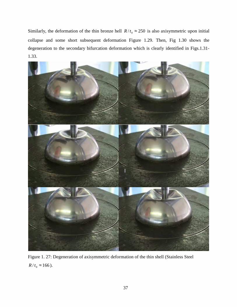
37
Similarly, the deformation of the thin bronze hell 250/ 0 ≈tR is also axisymmetric upon initial
collapse and some short subsequent deformation Figure 1.29. Then, Fig 1.30 shows the
degeneration to the secondary bifurcation deformation which is clearly identified in Figs.1.31-
1.33.
Figure 1. 27: Degeneration of axisymmetric deformation of the thin shell (Stainless Steel
166/ 0 ≈tR ).
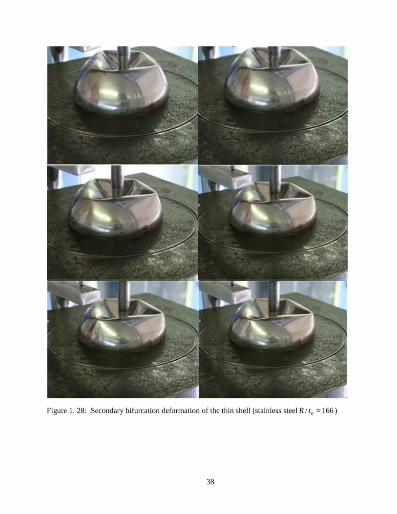
38
Figure 1. 28: Secondary bifurcation deformation of the thin shell (stainless steel 166/ 0 ≈tR )

39
Figure 1. 29: Initial buckling and axisymmetric post buckling of the thin shell (Bronze
)250/ 0 ≈tR

40
Figure 1. 30: Degeneration of the axisymmetric deformation of the thin shell (Bronze
)250/ 0 ≈tR .
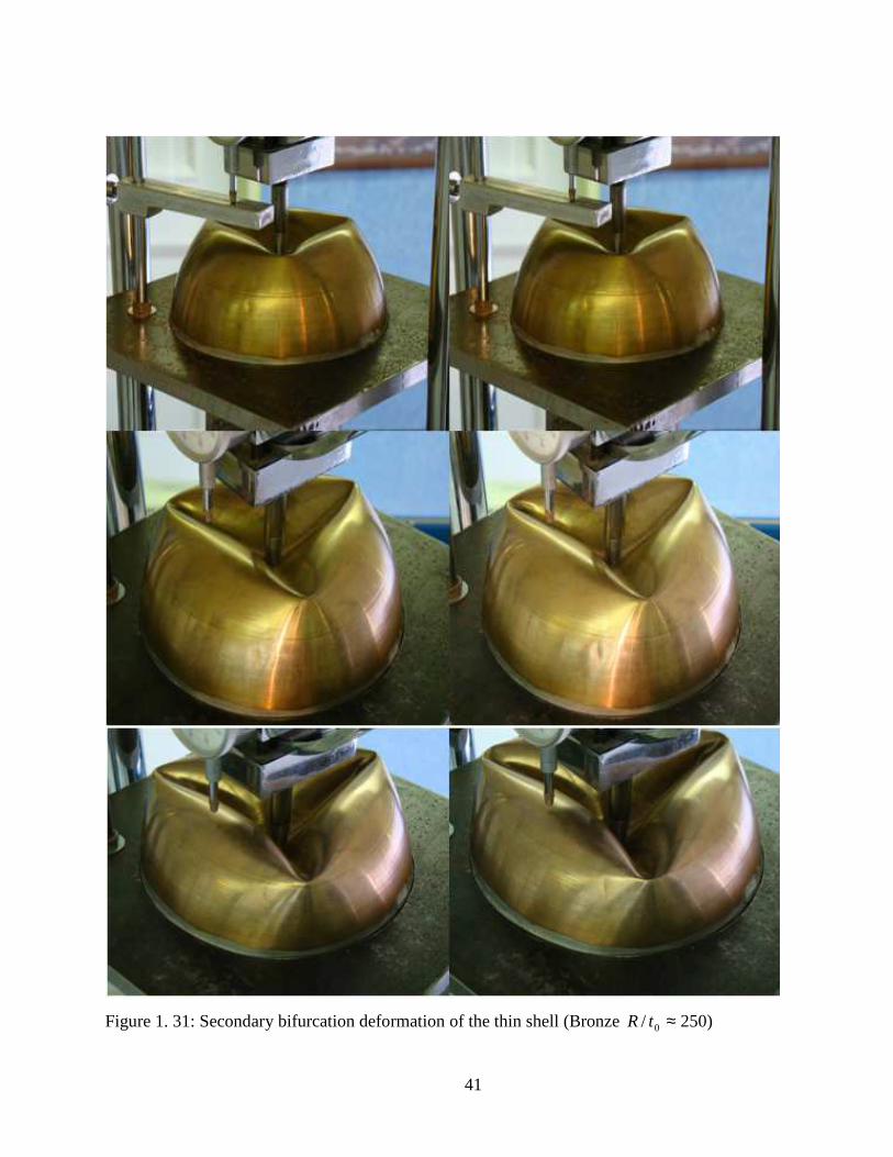
41
Figure 1. 31: Secondary bifurcation deformation of the thin shell (Bronze )250/ 0 ≈tR

42
Figure 1. 32: Different stages of the triangular with secondary bifurcation (Bronze 250/ 0 ≈tR )

43
Figure 1. 33: Final deformation of the thin shell (Bronze 250/ 0 ≈tR )
44
1.6 Results and Discussion
As it is seen in Fig.1.25 for relatively thick shell 100/0ptR , shell deformation pattern as
assumed in the analytical solution consists of a cone and torus which spread out
axisymmetrically from the apex with increasing load. Therefore, the analytical solution,
experimental findings and numerical results are expected to match for large amplitude of
deformations, Fig 1.34. However, when 100/0ftR , the deformation follows the same
axisymmetric pattern in the beginning. Then, the annular zone degenerates into various n-sided
polygon deformation modes and bifurcation in deformation pattern is observed (Figs.1.26-1.33).
In order to find bifurcation point in thin wall hemispherical shell ( 100/0ftR ) for which
the bending and membrane stresses are simultaneously important and assuming the boss pressure
to be uniformly distributed over the region of contact, new solution has been derived using
equilibrium approach.
Figs. 1.34, 1.40, and 1.43 give the load deflection curve for the copper alloy, Bronze, and
stainless steel shell respectively. The analytical solution results seem to be always slightly less
than the numerical solution because the finite element solution gives a lower bound on the
maximum displacements for a given set of forces and gives an upper bound on the maximum
stresses for a given set of displacements. The secondary bifurcation response is shown to yield
higher loads than the axisymmetric response for the same Rh value Fig 1.40 and 1.43, the
axisymmetric analytical solution may still be used for design of thin shells since it is on the
conservative side. Figs.1.35, 1.41, and 1.44 show the boss effect on the initial collapse load. Due
to ignoring the shell curvature in the small vicinity of the load, the collapse load is always
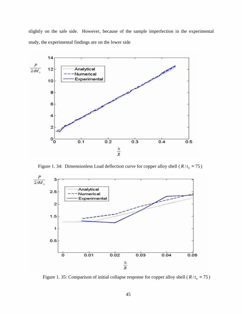
45
slightly on the safe side. However, because of the sample imperfection in the experimental
study, the experimental findings are on the lower side
Figure 1. 34: Dimensionless Load deflection curve for copper alloy shell ( 75/ 0 ≈tR )
Figure 1. 35: Comparison of initial collapse response for copper alloy shell ( 75/ 0 ≈tR )

46
Figure 1. 36: Dimensionless initial collapse load vs boss size for copper alloy shell ( 75/ 0 ≈tR )
Figure 1. 37: Dimensionless initial collapse load vs initial collapse angle for copper alloy
( 75/ 0 ≈tR )

47
Figure 1. 38: Initial collapse angle vs boss size for copper alloy ( 75/ 0 ≈tR )
Figure 1. 39: Dimensionless Load vs knuckle meridional angle in rad for copper alloy shell
( 75/ 0 ≈tR ).

48
Figure 1. 40: Dimensionless Load deflection curve for Bronze shell ( 250/ 0 ≈tR )
Figure 1. 41: Comparison of initial collapse response for Bronze shell ( 250/ 0 ≈tR )

49
Figure 1. 42: Dimensionless initial collapse load vs boss size for Bronze shell ( 250/ 0 ≈tR )
Figure 1. 43: Dimensionless Load deflection curve for Stainless Steel shell ( 166/ 0 ≈tR )

50
Figure 1. 44: Comparison of initial collapse response for Stainless Steel shell ( 166/ 0 ≈tR )
Figure 1. 45: Dimensionless initial collapse load vs boss size for Stainless Steel shell
( 166/ 0 ≈tR )

51
(h/R) vs (R/t)
00.10.20.30.40.50.60.70.80.9
1
100 120 140 160 180 200
(R/t)
(h/R
)
Bronze
Stainless Steel
Copper Alloy
Figure 1. 46: Numerical bifurcation point for Bronze, Stainless Steel, and Copper alloy versus
( 0/ tR ).

52
1.7 Conclusions
In this research the effect of the geometry change on the plastic buckling behavior of
hemispherical metal shells loaded inwardly at the apex has been studied theoretically,
numerically and experimentally. An analytical expression has been derived for plastic buckling
of hemispherical shell in a form which is especially convenient for application due to its
simplicity. In addition, it shows that a quite simple model of deformation at equilibrium is
sufficient to make predictions concerning postbuckling behavior of a moderately thick
hemispherical shell subjected to a concentrated load on top. The initial buckling load has been
shown to be highly depending on the radius of the loading boss. A formulation is used to
evaluate this effect based on the initial collapse of a simply-supported circular plate under
concentrated rigid boss. The results of initial buckling load formulation due to ignoring the
shell curvature in small vicinity of the loading actuator are always slightly on the safe side. It is
found that the shell carrying capacity after initial collapse increases continuously with the
deflection. The hemispherical shell deformation can be represented by a mathematical model
consisting of a cone and a torus which spread out symmetrically from the apex with
increasing load. The whole region of the shell forming the cone must be plastic to make this
deformation possible. The analytical solution results are shown to closely match those of
numerical and experimental values. It is also evident that larger boss size corresponds to higher
initial collapse load and larger dimple size. This solution is rigorously applicable for shells
having smaller values of 0/ tR (not exceeding approximately 100). This is because the
symmetry of the propagating annular zone about the vertical axis cannot be assumed throughout
the load-deflection response for large, 0/ tR . For 0/ tR greater than 100, the outer part of the

53
annular zone turns at to be unstable after a certain deformation level where the plastic part of
the shell degenerates into an n-sided polygon. For thin shell which 0/ tR is larger than 100, the
bifurcation point is approximately found using analytical solution as well. On the other hand, for
very thin shells ultimate load carrying capacity is limited by punch strength of the shell material.

54
Notation used in this chapter
a Radius of Circular Plate
c Radius of Circular Plate used to model behavior at bifurcation point
b Radius of Rigid Boss
0t Initial Shell Thickness
t Current Shell Thickness
0M Shell Plastic Moment/Unit Length in shell
φM Meridional Moment/Unit Length in shell
βM Circumferential Moment/Unit Length in circular plate
rM Radial Moment/Unit Length in circular plate
tM Tangential Moment/Unit Length in shell
ϕN Meridional Force/Unit Length in shell
βN Circumferential Force/Unit Length in shell
Q Transverse Shear Force /Unit Length in shell
0P Shell initial Collapse Load
P Shell Current Load
R Shell Radius
θ Knuckle Meridional Angle
φ Toroid Angle
ρ Knuckle Radius
h Vertical deflection of the apex of the hemispherical shell

55
CHAPTER 2 - Nondestructive Method to Predict the Buckling
Load in Elastic Spherical Shells
2.1 Introduction and Purpose of this chapter
As the variety and the quantity of shells increase, the determination of shell behavior
becomes more and more important. One of the most important things is to determine the
buckling load of shells either experimentally or theoretically.
The critical load for an axially loaded elastic structure is the load at which straight
(undeformed) and the deformed form of a structure are both possible. Therefore, a small
increment of this critical load causes a sudden deformation called buckling. In an initially
straight member, if the weight of member is neglected and no eccentricity exists, until the
buckling load is attained there is no transverse deformation theoretically. But this definition of
critical load holds true only in a theoretical sense. Because, in reality, due to the manufactural
imperfections, a very small eccentricity or non homogenity, which are unavoidable for most
cases from the first point of application of the load, transverse deformations begins. When the
critical load has been attained there will be excessive deformations. Therefore, the theoretical
minimum buckling load is not a reliable one, since the actual critical load is less than that.
Theoretically speaking, there are an infinite number of critical loads, but in practice only the
smallest one is necessary, since, at this load or slightly below that load buckling should be
expected. Accordingly, the target is to determine this minimum buckling load either theoretically
or experimentally.
56
The modern design technique goes into the model investigation, especially, for
complicated structures as shells. Since in most cases, the true behavior of the shell is not known
or very difficult to know, the best thing is to make some assumptions and then to verify these
assumptions by means of model tests. Accordingly, this chapter is investigating a possibility of
nondestructive method for finding the critical buckling load in spherical shells. For this purpose,
Southwell’s nondestructive method for columns is extended to spherical shells subjected to
uniform external pressure acting radially, and then by means of experiments, it is shown that the
theory is applicable to spherical shells with an arbitrary symmetrical loading. In addition,
Southwell’s nondestructive technique for columns is extended to the framed columns. Therefore,
a procedure is developed that the critical loads of columns in a multi-story frame can be
determined by using lateral deflections obtained through matrix formulation.
2.2 Southwell Method in Columns
If x is measured along the line of the thrust, and y defines the transverse deflection,
which is very small everywhere meaning that the small deformation theory is applicable, and
assuming P has a constant intensity over the span length L , writing the sum of the forces in
horizontal and vertical directions and the moments about an arbitrary point, (equilibrium
equations) the condition of equilibrium for the bent configuration may be obtained, Fig .2.1.
Summing up the forces in vertical direction and equating to zero;

57
Figure 2. 1: Column under compression force
( ) 00 =∆+∆++−→=↓+ ∑ xqVVVFy (2.1)
therefore, after taking the limit:
dx
dVq −= (2.2)
The sum of the moments,
( ) ( ) ( ) 022
=∆+∆+∆∆++∆+− yPxqxVVMMM (2.3)
taking the limit,
58
dx
dM
dx
dyPV =+ (2.4)
but since Mdx
ydEI −=
2
2
( ) qyPyEIdx
ydPq
dx
ydP
dx
dV
dx
Md =′′+″′′→+−=+=2
2
2
2
2
2
(2.5)
where EI is the flexural rigidity, P is the axial force and q is the lateral load. In the case
of zero lateral load, it is possible to write equilibrium equation as:
0=+′′ PyyEI (2.6)
calling, EIP=2α , the general solution equation will be:
( )0
sin xxAy −= α (2.7)
where Aand 0
x are two arbitrary constants of integration.
The condition that y must vanish at both ends of the strut will be realized if, 0sin =lα
which is possible for 0=α , but in that case, the strut will remain straight or in other words, there
will not be any deformation. The further solutions are l
nπα = where ...,.........3,2,1=n .
Substitution of this value into the equation EI
P=2α yields 2
22
l
n
EI
P π= or by substituting
the values ofn ,
22
2
,.......,9,4,1 nEI
Pl =π
(2.8)
For practical purposes, only the smallest value of that critical load is needed. Therefore,
using the smallest value ofn , which is one,

59
2
2
L
EIPcr
π= (2.9)
Suppose now that the strut is not quite straight initially, and let 0
y be the initial transverse
deflection of the strut. Then the equation of equilibrium for zero lateral loads will be;
( ) 02
0 0 yyypyyyEI ′′=+′′→=+′′−′′ α (2.10)
Provided that y vanishes at both ends of the strut. A general solution may be obtained by
expressing both y and 0
y in terms of Fourier’s series. Therefore;
∑∞
=
=1
sinn
n L
xnwy
π (2.11)
∑∞
=
=1
0 sinn
n L
xnwy
π (2.12)
Differentiating them with respect to x tweice,
∑∞
=
−=′′1
2
22
sinn
n L
xnw
L
ny
ππ (2.13)
∑∞
=
−=″1
2
22
0sin
nn L
xnw
L
ny
ππ (2.14)
Substituting back into the differential equation (2.10),
22
22
1πα
n
L
ww n
n
−= (2.15)
If nP is the thn − critical load, then2
22
L
EInPn
π= .Therefore,
n
n
n
P
Pw
w−
=1
(2.16)

60
AsP approaches to its first critical value1P , 1w will be very largely magnified, while 2w
will be approximately in the ratio four over three, 3w nine over eight and so on.
This result explains why as the load is increased, every strut appears to bent into a sine
wave of one bay, other harmonics are present, but they are very little magnified by the load,
whereas the first harmonic soon becomes large. Also in that case, from the differential equation
it is possible to notice that the deflection begins from the first application of the load, since the
differential equation is not homogeneous anymore due to the consideration of the initial
imperfections, which are almost unavoidable in practice.
The deflection of the strut at its centre may be written as;
∑∞
=
−+−=×=1
531 ........2
sinn
n wwwL
L
nw
πδ (2.17)
or
1
11
1P
Pw
w−
=≅δ (2.18)
Thus provided that the above mentioned assumptions hold true, the load-deflection curve
is a rectangular hyperbola having the axis of P , and the horizontal line crPP = as asymptotes.
(See Fig. 2.2a)

61
Figure 2. 2: Load Deflection curve in Southwell Method
Now, if a hyperbola passes through the origin and has asymptotes of equations.
0
0
=−=+
βα
y
x (2.19)
The equation of this hyperbola will be:
0=+− yxxy αβ (2.20)
or dividing by y ;
0=+− αβ yxx (2.21)
calling vyx = the equation of the hyperbola becomes;
0=+− αβvx (2.22)

62
which is a straight line. Therefore, if x is plotted againstv , the inverted slop dv
dxis the
measure of the smallest critical load (See Fig 2.2b).
If instead of having an initial curvature, an initial eccentricity ehas appeared since in the
case of a single lateral load Q the deflected shape may be defined as;
∑∞
=
−
=1 2
3
3sinsin
11
n
n
L
xn
L
cn
P
Pnn
EI
QLy
πππ
(2.23)
where c is the distance between the support and the point of application of the load. Making
c infinitely small, the condition of bending by a couple is obtain. Therefore, using the notation
QcM = ;
∑∞
=
−
=1 2
2
3sin
12
n
n
L
xn
PPnnEI
MLy
ππ
(2.24)
is obtained. For two moments applied at both ends, by superposition;
( )
−+
−
= ∑∞
= L
xLn
L
xn
PPnnEI
MLy
n
n
πππ
sinsin12
1 2
2
3 (2.25)
and the deflection at the midspan is:
+
−
−−
= ..............
93
1
1
14
3
1
2
3
P
PPPEI
ML
πδ (2.26)
Since due to symmetry, the even terms do not appear.
If the couples at both ends are caused due to the small eccentricity eof the applied axial loads
P , then calling MPe=

63
+
−
−−
= ...........93
1
1
14
31
1P
PPPP
Pe
πδ (2.27)
As P reaches 1P the ratio 1P
P reaches to unity. So, while the first term approaching to
infinity, the others approach to zero therefore,
11 1
14
PPP
Pe
−=
πδ (2.28)
or in a more compact form,
1
14
1 −=
PP
e
πδ (2.29)
For a more general case of combination of both an eccentricity and curvature:
1
14
1 −
+=
PP
ewn π
δ (2.30)
which is analogous to the original equation:
1
1
1 PP
w
−=δ (2.31)
The main advantage of the method lies in its generality and simplicity. In all ordinary
examples of elastic instability the equation
00 =+
″−′′ PyyyEI (2.32)
governs the deflection as controlled by its initial value, provided that both are small. It
follows that the deflection is related with the applied load by an approximate equation of the
hyperbolic form

64
crPPw
w−
=≅1
11δ (2.33)
2.3 Agreement of Test Results in Columns
As stated in the preceding section, the relation between measured load and deflection will
not be hyperbolic if the deflections are so large that the elasticity of the material is impaired;
moreover, when the deflections are large the approximations will not hold true. On the other
hand, if both the deflections and loads are small, the exact measurements will not be possible.
Thus, same scatter of the observational points must be expected. Moreover, in this range 1w (the
first term of the Fourier series) does not necessarily dominate the expression for deflection
(Southwell 1932).
The data required for a satisfactory test is related values of load and central deflection for
columns which have been loaded as axially as possible.
The recorded observations of this nature are given by T. Von Karman (1909) in an
inaugural dissertation published in 1909. In his paper, the experimental struts are classified in
three groups, described relatively as slender, medium or thick. Slender struts having a k1 ratio
greater than 90 and for medium struts the slenderness ratio ranges between 45 and90 , and thick
struts are those for which the slenderness ratio is less than 45.
In the slender group, Von Karman tested eight struts, numbered 1, 2, 3a, 3b, 4a, 4b, 5,
and 6. These have been analyzed by R. V. Southwell (1932) in Table 2.1 and Fig. 2.3 exhibiting
the relation of x tov . In some instances the initial observations have been rejected in estimating
the best fitting straight lines; such observations are distinguished in the table by asterisks. The

65
remaining observations have been analyzed by the method of least squares by R.V. Southwell, in
order that the best fitting lines might be determined without introduction of personal judgment.
Table 2.2, gives the values of slope as determined from the best fitting lines. This table
shows that the agreement with theory in regard to the critical load is in fact very close. The
actual value of the modulus of elasticity, measured by Karman is 2170000 2cmkgf .
As applied to the struts in Karman’s medium and thick groups, the method failed for the
reason that practically every observation related to deflections, which can be shown to have
involved in elastic failure of the material. It, thus, appears that the method has given good results
in every case where these could be expected, but that only trial can show whether in any instance
sufficient observations can be taken of deflection which on the one hand are large enough to give
reasonable certainty of ,v and on the other hand, are not so large that material is still elastic.
One of the struts tested by Prof. Robertson (1912) was loaded with such small
eccentricity by R. V. Southwell as to provide a fair test of the method. Table 2.3 presents the
analysis of this case, and related values.
As it is seen from that figure, the plotted points fall on two distinct straight lines; the
first, covering values of the measured deflection ranging from 7 to 18 thousands of an inch,
indicated an initial deflection of about 0.01 inch and a critical load of 14.5 tons, which is some
ten percent in excess of the value 12960 kgs obtained from Euler’s theoretical expression when
modulus of elasticity is given the value 3.13 2intons , which was measured by Prof. Robertson.
The second test representation values of the measured deflection in excess of 18 thousandths of
an inch (of which 0.0064 inch is the amplitude of the first harmonic in the Fourier series for the

66
specified eccentricity of 0.005 inch) and a critical load of about 12.9 tons, which is less than half
percent in error as compared with the theoretical figure.
Table 2. 1: Nos. 1, 2, 3a, 3b, 4a, 4b, 5 and 6. Mild steel: Modulus of
Elasticity 22170000cm
kgf=
Strut No:1
P , end load in kilograms x , measured deflection (mm) 610×= Pxv
2260 0.01 4.43
3020 0.025 8.28
3170 0.04 12.62
3320 0.06 18.07
3470 0.09 25.94
3620 0.25 69.06
Strut No:2
P , end load in kilograms x , measured deflection (mm) 610×= Pxv
4520 0.02 4.43
4830 0.05 10.35
5130 0.11 21.44
5280 0.24 45.45
Strut No:3a
P , end load in kilograms x , measured deflection (mm) 610×= Pxv
6030 0.01 1.66
7540 0.03 3.98
8290 0.11 13.27
8520 0.52 61.03
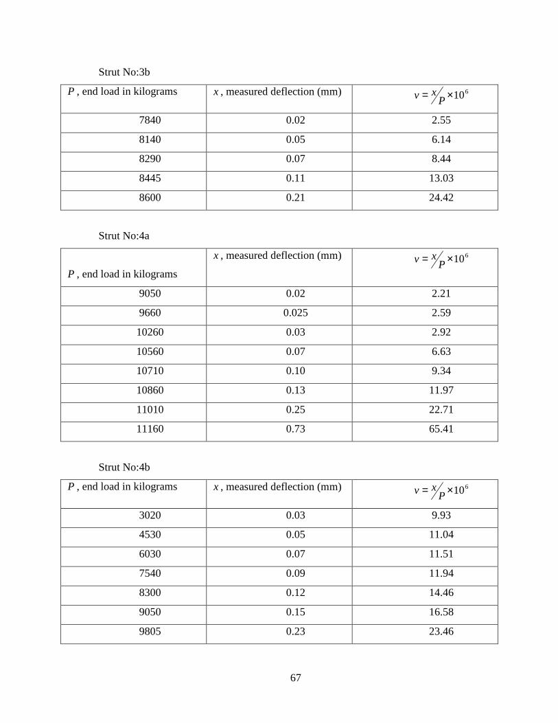
67
Strut No:3b
P , end load in kilograms x , measured deflection (mm) 610×= Pxv
7840 0.02 2.55
8140 0.05 6.14
8290 0.07 8.44
8445 0.11 13.03
8600 0.21 24.42
Strut No:4a
P , end load in kilograms
x , measured deflection (mm) 610×= Pxv
9050 0.02 2.21
9660 0.025 2.59
10260 0.03 2.92
10560 0.07 6.63
10710 0.10 9.34
10860 0.13 11.97
11010 0.25 22.71
11160 0.73 65.41
Strut No:4b
P , end load in kilograms x , measured deflection (mm) 610×= Pxv
3020 0.03 9.93
4530 0.05 11.04
6030 0.07 11.51
7540 0.09 11.94
8300 0.12 14.46
9050 0.15 16.58
9805 0.23 23.46

68
9960 0.26 26.10
10110 0.29 28.8
10260 0.33 32.16
10410 0.41 39.39
10560 0.52 49.24
10710 0.71 66.29
10860 1.46 134.44
Strut No:5
P , end load in kilograms x , measured deflection (mm) 610×= Pxv
9050 0.01 1.105
10560 0.03 2.84
10860 0.05 4.67
11160 0.07 6.27
11470 0.10 8.72
11770 0.15 12.74
12070 0.22 18.23
12370 0.30 24.25
12520 0.45 35.94
Strut No:6
P , end load in kilograms x , measured deflection (mm) 610×= Pxv
10560 0.01 0.95
12070 0.04 3.31
12370 0.08 4.85
12670 0.10 7.89
12970 0.15 1.57
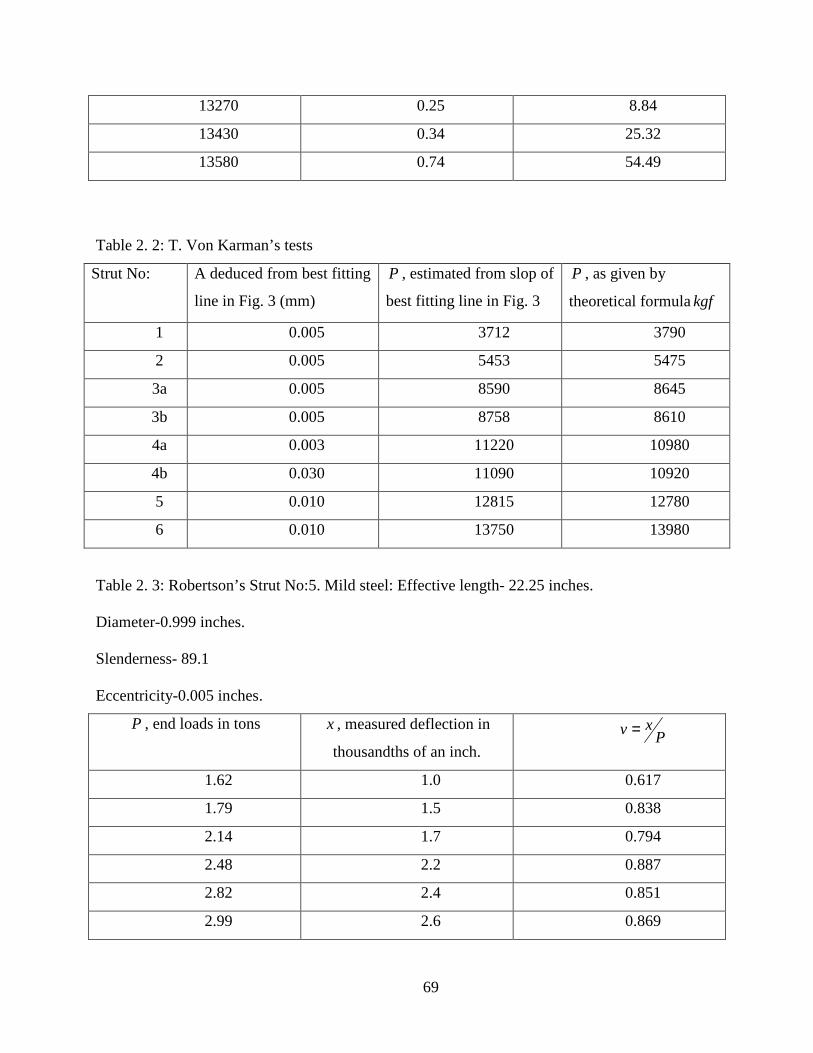
69
13270 0.25 8.84
13430 0.34 25.32
13580 0.74 54.49
Table 2. 2: T. Von Karman’s tests
Strut No: A deduced from best fitting
line in Fig. 3 (mm)
P , estimated from slop of
best fitting line in Fig. 3
P , as given by
theoretical formulakgf
1 0.005 3712 3790
2 0.005 5453 5475
3a 0.005 8590 8645
3b 0.005 8758 8610
4a 0.003 11220 10980
4b 0.030 11090 10920
5 0.010 12815 12780
6 0.010 13750 13980
Table 2. 3: Robertson’s Strut No:5. Mild steel: Effective length- 22.25 inches.
Diameter-0.999 inches.
Slenderness- 89.1
Eccentricity-0.005 inches.
P , end loads in tons x , measured deflection in
thousandths of an inch. P
xv =
1.62 1.0 0.617
1.79 1.5 0.838
2.14 1.7 0.794
2.48 2.2 0.887
2.82 2.4 0.851
2.99 2.6 0.869

70
3.16 2.8 0.886
3.34 3.0 0.898
3.50 3.27 0.934
3.68 3.64 0.989
3.86 4.00 1.037
4.02 4.24 1.060
4.19 4.46 1.063
4.36 4.68 1.078
4.53 4.81 1.063
4.70 4.94 1.051
4.90 5.07 1.028
5.13 5.66 1.106
5.56 6.32 1.140
5.99 6.97 1.163
6.42 7.80 1.218
6.84 8.95 1.310
7.27 9.84 1.358
7.70 11.18 1.450
8.12 12.75 1.572
8.55 14.08 1.647
8.98 15.88 1.768
9.4 18.34 1.951
9.83 21.91 2.222
10.25 26.27 2.563
10.68 32.47 3.040
11.11 41.17 3.706

71
2.4 An Extension of the Southwell Method for columns in a Frame structure
This section shows an approach whereby the critical loads of columns in a multi-story
frame can be determined by using lateral deflections obtained through matrix formulation. The
deflection data of columns in a multi-story frame are obtained by including the effect of presence
of axial loads in the member and structure stiffness matrices. Effects of initial bending moments
are also included. The results prove that Southwell plotting technique used to determine the
critical load of single column is also applicable to framed columns.
2.4.1 Formulation of the Governing Equations
For a single column, formulations can be made directly to obtain the critical load. Simple
formulations can also be extended to simple portal frames as done by Zweig (1968). When the
problem arises to analyze and design a tall building subjected to gravity and lateral loads,
however, use of modern matrix methods becomes necessary.
Because of large number of degrees of freedom involved in a multi-story building frame,
one is confronted with a correspondingly large number of equations which can be repeatedly
solved only by use of matrix method. When buckling is involved then efficient matrix
formulations can be made using slope deflection equations modified by stability functions.

72
Figure 2. 3: Notation for member and structure
With reference to a notation system shown in Fig.2.3, member stiffness equations 1, 2, 3,
and 4 are formed using equations of equilibrium (Bleich (1952)).
The axial force equation is given by:
( )111 aba uu
L
EAf −= (2.34)
The shear force equation is given by
( )22332 533232
1266abbaa uu
L
EIu
L
EIu
L
EIf −
−
+
= βββ (2.35)
The bending moment equations are given by
( )22333 3221
624abbaa uu
L
EIu
L
EIu
L
EIf −
−
+
= βββ (2.36)
( )22333 3212
642abbab uu
L
EIu
L
EIu
L
EIf −
−
+
= βββ (2.37)

73
where f is the end force, u is the end displacement, the subscripts i and j refer to the
particular end of the member and the direction respectively, iβ represents corresponding
stability functions IAE ,, and L are modulus of elasticity, cross sectional area, moments of
inertia and length of the member respectively.
Stability functions iβ have been widely publicized (Gregory (1968)).
They may be concisely expressed as (see appendix C)
( )αα
ααα−
−=tan
2cot21S (2.38)
ααααα
2cos22sin
2sin2
−−=C (2.39)
41S=β (2.40)
22SC=β (2.41)
( )6
13
CS +=β (2.42)
ααβ cot4 =
435 .βββ = (2.43)
where EP
P2
1=α with P being the axial load on a given structural member and
EP being the Euler Load for that particular member.
By use of appropriate transformation matrices, the member stiffness equations are
transformed to a global coordinate system. Structure stiffness equations are then formed by using
the equations of compatibility.
The steps leading to the computer program are summarized as follows:

74
a) For a given frame adopt numbering system for members and joints, formulate the
number equations, transform them to the structure coordinate system, and formulate the
structure stiffness matrix by using compatibility equations.
b) Adopt a proportionate multiplier of load, λ , for a given external loading pattern.
Then for any value of λ , formulate an external force vector. In the external force vector, the
fixed end moments of each member must be modified for the presence of axial load in that
member. This is done by deriving the appropriate stability function corresponding to the
particular lateral loading on the member.
The stability function corresponding to a uniformly distributed load over the complete
length of a member is derived as .1
3β This function is used to modify the fixed end moments
in the force vector due to the loading of this frame.
c) For any value λ of a loading pattern, initial solution necessitates all iβ be set to
unity (i.e. axial forces 0= ). By using an invert subroutine, solve the system of equations for
the unknown displacements. With the displacements and using equation 1, a vector of axial
forces of members is obtained. For each member, iβ values are calculated and equations
(2.35), (2.35) and (2.36) are modified in order to reformulate the member and structure
equations.
d) The iteration is continued until elements of force vectors and displacement vectors of
two successive iterations are correspondingly close to one another. The control point in
continuing further iterations is the test value of the determinant of the stiffness matrix.
If the values of the determinant are positive, then according to the principle of
positive definiteness for stability, further iteration becomes possible.

75
e) Once the final set of displacements and forces for a value of λ are obtained, then
they are stored further use.
f) Steps c, d and e are repeated for a different value ofλ .
Solutions for the structure are completed; end displacements and end forces have
been obtained. Now, it is possible to further study the members.
2.4.2 Member Formulations and Solutions
For a straight prismatic member, the general equation of equilibrium is given by
00
22 1=
−″+∫
L
aIV dxqufEIu let Pfa =
1 (2.44)
where q is the intensity of the lateral load on the member.
Solution of equation (2.44) is
211112 2
12sin
2cos x
P
qDCxx
LBx
LAu ×++++= αα
(2.45)
In the member axis system ( )321 ,, xxx of each member, the boundary conditions, the final
end forces and displacements corresponding to each value of λ of a loading pattern (obtained in
step e of the procedure) are:
End a End b
444444 8444444 76
444444 8444444 76
Displacements Forces Displacements Forces
=
3
2
1
a
a
a
a
u
u
u
ui
=
3
2
1
a
a
a
a
f
f
f
fi
=
3
2
1
b
b
b
b
u
u
u
ui
=
3
2
1
b
b
b
a
f
f
f
fi

76
Using these, the coefficients of equations of equation (2.45) can be determined.
Let L
wtrααα 2
,2cos,2sin === and EP
P2πα = then,
−
−=
−P
qLu
P
qLu
u
u
D
C
B
A
wtwr
Lrt
w
b
b
a
a
3
2
3
2
2
01
1
010
1001
(2.46)
Knowing the right hand side of equation (2.46), it is possible to determine the
coefficients and use them in equation in equation (2.45) to calculate the lateral displacement 2u at
any point 1x of the member.
2.4.3 Southwell Plot
Using the computer program, for a given frame and a loading pattern, all information
regarding the axial forces and displacements at different points of columns are calculated and
stored. For every column member, plotting axial load/lateral deflection ratio against axial load
for various points within member length yields straight lines converging to one point on the axial
load axis. This is the elastic critical load, cr
P of the column under the given loading of the frame.
The critical load corresponds to that value of the axial load when the displacements approach
infinity.
A curve fitting routine greatly reduces the amount of work involved in determining a
Southwell Plot which leads to a critical load.

77
2.4.4 Case Study
In order to demonstrate the procedure, the frame designed by Wood and investigated by
Bowles and Merchant (1956) is adopted. A loading pattern is accepted and the solution is carried
out. Fig 2.4 gives the dimensions and the cross section profiles of members of the frame. Also, is
illustrated the numbering system used in the computer program. Table 2.4 gives the
characteristics of the members of this frame according to the numbering system of Fig 2.4.
The loading pattern used is given in Fig. 2.5. In table 2.5 are given the results for member
8 for various values of λ of this loading pattern of the frame. The Southwell Plots are illustrated,
and as seen in Fig. 2.5, the i
P∆ vs. P curves yield straight lines that converge to the same point
defining the critical load, crP which is equal to 3380 kips.

78
Table 2. 4: Characteristics of Wood’s Frame
Members ( )inL ( )4inI ( )2inA ( )ksiPE
1 180 322 20.78 2942.6
2 177 322 20.78 3043.2
3 177 271 18.28 2561.2
4 189 208 14.71 1724.1
5 183 115 10.30 1016.8
6 180 602 22.30 5501.4
7 177 460 19.30 4347.5
8 177 378 18.78 3572.5
9 189 221 17.03 1831.9
10 183 492 10.30 4349.9
11 180 322 20.78 2942.6
12 177 322 20.78 3043.2
13 177 271 18.28 2561.2
14 189 208 14.71 1724.1
15 183 115 10.30 1016.8
16 279 1226 19.12
17 279 1226 19.12
18 279 1226 19.12
19 279 1226 19.12
20 279 492 13.24
21 279 1226 19.12
22 279 1226 19.12
23 279 1226 19.12
24 279 1226 19.12
25 279 492 13.24
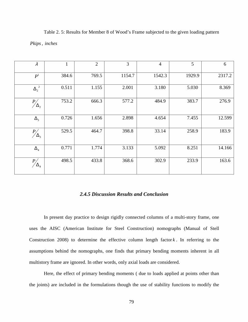
79
Table 2. 5: Results for Member 8 of Wood’s Frame subjected to the given loading pattern
Pkips, inches
λ 1 2 3 4 5 6
1P 384.6 769.5 1154.7 1542.3 1929.9 2317.2
22∆ 0.511 1.155 2.001 3.180 5.030 8.369
2∆P 753.2 666.3 577.2 484.9 383.7 276.9
3∆ 0.726 1.656 2.898 4.654 7.455 12.599
3∆P 529.5 464.7 398.8 33.14 258.9 183.9
4∆ 0.771 1.774 3.133 5.092 8.251 14.166
4∆P 498.5 433.8 368.6 302.9 233.9 163.6
2.4.5 Discussion Results and Conclusion
In present day practice to design rigidly connected columns of a multi-story frame, one
uses the AISC (American Institute for Steel Construction) nomographs (Manual of Stell
Construction 2008) to determine the effective column length factork . In referring to the
assumptions behind the nomographs, one finds that primary bending moments inherent in all
multistory frame are ignored. In other words, only axial loads are considered.
Here, the effect of primary bending moments ( due to loads applied at points other than
the joints) are included in the formulations though the use of stability functions to modify the

80
fixed end moments ( for uniformly distributed load, 3
1β is used). Therefore, the procedure leads
to a more rational evaluation of the critical load.
Once the critical load has been determined, the effective length factor k is given by
cr
EP
Pk =
For member 8 of the frame in the example, the Eular load EP is in Table 2.4. Then k is
found to be equal to 1.03. AISC nomographs yield k equal to 1.14.
The technique demonstrates that there is an effect of the loading pattern of a frame on the
load carrying capacity of a column in that frame. This fact has been long discussed, and the
German Codes partially take into account. Zweig (1968) proved that load carrying capacity
changes when two different values of external loads are applied to a portal frame.
In conclusion, by using matrix formulations, the Southwell plotting technique is proved
to be applicable to determine the critical loads of columns in multistory frames under given
loading patterns.
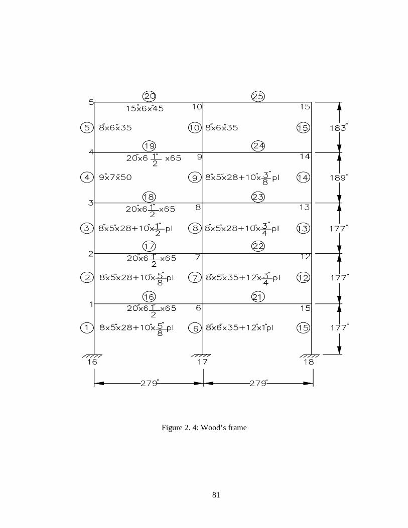
81
Figure 2. 4: Wood’s frame

82
Figure 2. 5: Loading of frame, Soutwell plot for member 8

83
2.5 The Southwell Method Applied to Shells
To apply the Southwell method of predicting the critical load without disturbing the
model, a uniformly compressed spherical shell is considered. If a spherical shell is submitted to a
uniform external pressure, it may retain its spherical form, and undergo a uniform compression
whose magnitude is in this case;
02t
pa=σ (2.47)
So, for values of pressure increasing from zero, the shell will at first deform in a rather
uniform manner. This process persists until the external pressure,p , reaches a certain critical
value, crp , called the initial buckling pressure. At this value of pressure the shell no longer
deforms in a uniform manner but jumps or snaps into another non-adjacent equilibrium
configuration. The pressure to which the shell jumps is called the final buckling pressure. Thus,
if the pressure increases beyond a certain limit, the spherical form of equilibrium of the
compressed shell may become unstable, and buckling then occurs. In order to calculate this
critical pressure, the buckled surface is assumed to be symmetrical with respect to the diameter
of the sphere. But before going into the detail of the buckling problem it is advisable first to
consider the bending theory of shells.

84
2.5.1 Deformation of an Element of a Shell of Revolution
In the Fig. 2.6 let ABCD represents an infinitely small element taken from a shell by two
pairs of adjacent plans normal to the middle surface of the shell and containing its principle
curvature( Timeshenko et.al (1961) and Timeshenko et al. (1959)).
Taking the coordinate axes xand y tangent at an arbitrary point oof the middle surface
and the axis znormal to the middle surface, the element may be defined. In bending theory of
shells, it is assumed that, the linear elements, which are normal to the middle surface of the shell
remain straight and become normal to the deformed middle surface of the shell. Thus the law of
variation of the displacements through the thickness of the shell is linear (Novozhilov (1959)).
During bending, the lateral faces of the element ABCDhave rotation and displacement;
superposing and first considering rotation only with respect to their lines of intersection with the
middle surface. The unit elongations of a thin lamina at a distance z from the middle surface are;
−
′−−=
xxx
x rrr
zz 11
1ε
(2.48)
−
′−−=
yyy
y rrr
zz 11
1ε (2.49)
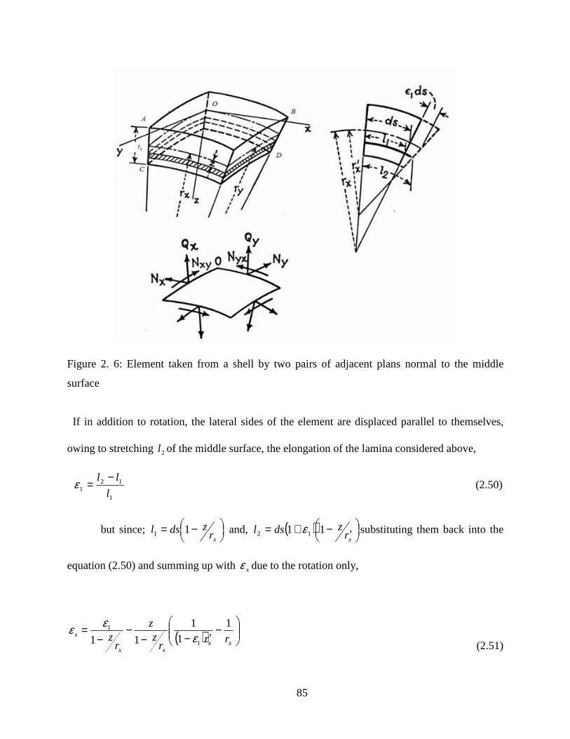
85
Figure 2. 6: Element taken from a shell by two pairs of adjacent plans normal to the middle
surface
If in addition to rotation, the lateral sides of the element are displaced parallel to themselves,
owing to stretching 2l of the middle surface, the elongation of the lamina considered above,
1
121 l
ll −=ε (2.50)
but since;
−=
xrzdsl 11 and, ( )
′−+=xr
zdsl 11 12 ε substituting them back into the
equation (2.50) and summing up with xε due to the rotation only,
(2.51) ( )
−
′−−−
−=
xxxx
x rrr
zz
rz
1
1
1
11 1
1
εεε

86
and similarly,
( )
−
′−−−
−=
yyyy
y rrr
zz
rz
1
1
1
11 2
2
εεε (2.52)
Since the thickness 0t of the shell always will be assumed small in comparison with the
radius of curvature, the quantities xr
z and yr
z may be neglected in comparison with unity.
Also neglecting the effect of elongations 1ε and 2ε on the curvature the expressions become,
−
′−=
xxx rr
z11
1εε (2.53)
and,
−
′−=
yyy rr
z11
2εε (2.54)
Assuming that, there are no normal stresses between laminas 0=zσ is obtained. Then,
from the well known formulae;
( )yxx
E υεευ
σ +−
= 21 (2.55)
( )xyy
E υεευ
σ +−
=21
(2.56)
Therefore, substituting the values of strain components;

87
( )( )yxx zE υχχυεευ
σ +−+−
= 2121 (2.57)
( )( )xyy zE υχχυεευ
σ +−−−
= 1221 (2.58)
are obtained. Since the thickness of the shell is very small, the lateral sides of the element
may be considered as rectangles. Therefore the corresponding normal forces acting to the
centroit of the side will be;
for 1=dy (2.59)
( )∫−
−−
==2
2
1220
0
01
t
tyy
EtdzN υεε
υσ for 1=dx (2.60)
and the moments, ( )∫−
−−==2
2
0
0
t
tyxxx DdzzM υχχσ , and ( )∫
−
−−==2
2
0
0
t
txyyy DdzzM υχχσ in which
( )∫−
−=
−=
2
2
2
302
2
0
01121
t
t
Etdzz
ED
νυ .
Now knowing that the shearing stresses are also acting on the lateral sides of the element in
addition to the normal stresses. If γ is the shearing strain in the middle surface and dxxyχ the
rotation of the edge BC relative to −z axes, ( )Gz xyxy χγτ 2−= is obtained. Also knowing that
∫−
=2
2
0
0
t
txzx dzQ τ , ∫
−
=2
2
0
0
t
tyzy dzQ τ , ∫
−
==2
2
0
0
t
txyxyyx dzNN τ and ∫
−
==−2
2
0
0
t
txyyxxy dzzMM τ one may find,
( ) xyyxxy DMM χυ−=−= 1 ,and ( )υγ
+==
120Et
NN yxxy
( )∫−
+−
==2
2
2120
0
01
t
txx
EtdzN υεε
υσ

88
Thus assuming that during bending of a shell of revolution the linear elements, normal to
the middle surface the resultant forces yx NN , and xyN and the moments, xM , yM , and xyM may
be expressed in terms of six quantities; three components of strain1ε , 2ε , and γ of the middle
surface of the shell and the three quantities xχ , yχ , and xyχ representing the changes of
curvature and the twist of the middle surface of the shell.
2.5.2 Equations of Equilibrium of a Spherical shell
Due to the symmetrical deformation, one of the displacement components vanishes, and
the others are only the functions of angleθ . Therefore;
( )θ1fu =
0=v
( )θ2fw =

89
Figure 2. 7: Spherical shell element and corresponding forces
In the case of symmetrical deformation, there are only three equations to be considered as
the projections of forces on thex , and zaxes and moments of forces with respect the −y axes.
Therefore after simplification, the three equations of equilibrium become;
( ) 0cot =−−+ xyxx QNN
d
dN θθ
(2.61)
0cot =++++ paNNQd
dQyxx
x θθ
(2.62)

90
( ) 0cot =−−+ aQMMd
dMxyx
x θθ
(2.63)
2.5.3 Equations of Equilibrium for the Case of Buckled Surface of the Shell
In writing the equations of equilibrium for the case of buckled surface of a shell, which is
assumed symmetrical with respect to any diameter of the shell, the small changes of the angles
between the faces of any element such as ABCDdue to the deformation has to be considered.
Since there is symmetry of deformation, the rotation will only be with respect to −y axes. For
the face OC , this deformation is;
θad
dw
a
u + (2.64)
Thus the angle between the faces OC and ABafter deformation becomes;
θθθ
θ dad
dw
a
u
d
dd
++ (2.65)
The faces AOand BCowing to symmetry of deformation, rotate in their own planes by
an angle,
+−θad
dw
a
u (2.66)

91
Such a rotation in the plane of the face BChas components with respect to the xand
zaxis equal to; ψθθ
dad
dw
a
ucos
+ and, ψθθ
dad
dw
a
usin
+− respectively. Thus after
deformation, the direction of the face BCwith respect to the face ADmay be obtained by the
rotation of the face AOwith respect to the x and zaxis through the
angles, ψθθ
ψθ dad
dw
a
ud cossin
++ and, ψθθ
ψθ dad
dw
a
ud sincos
+− respectively.
Using the above derived angles instead of the initial ones; ,θd ,sin ψθd and ,cos ψθd the
equations of equilibrium of the element OABCbecome;
( ) 0cot2
2
=
+−
++−−+a
w
ad
wdQ
ad
dw
a
uNQNN
d
dNxyxyx
x
θθθ
θ (2.67)
0cot.cot2
2
=
++
++++++ θ
θθθθ
θ ad
dw
a
uN
ad
du
ad
wdNpaNNQ
d
dQyxyxx
x (2.68)
( ) 0cot =
++−−+θ
θθ ad
dw
a
uMaQMM
d
dMyxyx
x (2.69)
In this case;
a
w
ad
du −=θ
ε1 (2.70)
a
w
a
u −= θε cot2 (2.71)
θθχ
da
du
da
wdx 222
2
+= (2.72)
θθ
χ cot22
+=da
dw
a
uy (2.73)

92
The differential equation of equilibrium developed have above are based on Love’s
general theory of small deformations of thin shells which neglects stresses normal to the middle
Surface of the shell and assumes that the planes normal to the undeformed middle surface remain
normal to the deformed middle surface.
Figure 2. 8: Meridian of a spherical shell before and after buckling

93
2.5.4 Buckling of Uniformly Compressed Spherical Shells
If a spherical shell is submitted to a uniform external pressure, there will be a uniform
compression whose magnitude is;
02t
pa=σ
Let vu, and w represent the components of small displacements during buckling from the
compressed spherical form, then xN and yN differ little from the uniform compressive force
2pa and they become,
xx Npa
N ′+−=2
(2.74)
yy Npa
N ′+−=2
(2.75)
where xN′ and yN′ are the resultant forces due to small displacements vu, and .w
Also, considering the small change of pressure on an element of the surface, due to the
stretching of the surface, p becomes ( ).1 21 εε ++p Therefore substituting equations (2.74) and
2.75) back into the differential equations of equilibrium (2.67), (2.68), and (2.69) and
simplifying and neglecting the small terms, such as the products of ,xN′ yN′ and xQ with the
derivations of vu, and ;w
( ) 05.0cot =
+−−′−′+′
θθ
θ ad
dw
a
upaQNN
d
Ndxyx
x (2.76)
0cot5.05.02
cotcot2
2
=
+−
+−
−++′+′++θ
θθθ
θθ
θθ ad
dw
a
upa
ad
wd
d
dupa
a
w
a
u
ad
dupaNNQ
d
dQyxx
x (2.77)

94
( ) 0cot =−−+ aQMMd
dMxyx
x θθ
(2.78)
From the Equation (2.78):
( )a
MMad
dMQ yx
xx
θθ
cot−+=
Substituting xQ into the Equations (2.76) and (2.77);
−+−−
=′a
w
au
a
w
ad
duEtNx
θυθν
cot
1 20 (2.79)
( )
−+−−
=′ wd
duwu
a
EtN y θ
υθν
cot1 2
0 (2.80)
+++−= θθ
υθθ
cot2
2
2 d
dwu
d
wd
d
du
a
DM x (2.81)
++
+−=2
2
2cot
θθυθ
θ d
wd
d
du
d
dwu
a
DM y (2.82)
Now introducing two dimensionless parameters, α and φ which are defined as;
( )2
20
02
2
12
1
a
t
Eta
D =−= υα and, ( )
0
2
2
1
Et
pa υφ −= and using the elastic law to express the forces and
moments in terms of u and wone obtains;

95
( ) ( ) ( ) ( )
0
cotcot1cotcot1 22
2
3
32
2
2
=
−−
+−+++−
′+−++
θφ
θθυ
θθ
θα
θυθυ
θθ
θα
d
dwu
d
dw
d
wd
d
wd
d
dwu
d
du
d
ud
(2.83)
( ) ( ) ( )
( ) ( ) ] 0cot4cotcot2cotcot1cot2
cot2cotcot1cot22cot1
2
22
2
22
3
3
4
422
2
2
3
3
=
+++−−−+−−+++−
−+−−+++−−+
−++
θθθθφ
θθυθ
θθυ
θθ
θθυθ
θθυ
θθ
θαθ
θυ
d
wd
d
dww
d
duu
d
dw
d
wd
d
wd
d
wdu
d
dug
d
ud
d
udwu
d
du
(2.84)
These two equations may be simplified by neglecting in comparison with unity in the first
term, since the shell is thin, and therefore at0 ratio is very small. Also, due largely to angular
displacement χ we make good use of this situation by introducing an auxiliary variable U such
that θψ
d
du −= . Thus, the expressions in the brackets become identical. Then using the symbol
H for the operation;
( ) ( ) ( ) ( ).........2.....
cot.....
2
2
++=θ
θθ d
d
d
dH
Equation (2.83) may be written as follows,
( ) ( ) ( )( ) ( ) ( )[ ] 011 =+−+−++−+ wwwwHHd
d ψφυαψυαψθ
The forth term, containing the factor, may be neglected in comparison with the third.
Integrating this equation with respect to θ and assuming the constant of integration is equal to
zero;
( ) ( ) ( )( ) ( ) 01 =+−++−+ wwwHH ψφψυαψ (2.85)

96
And similarly for Equation (2.84) ;
( ) ( ) ( ) ( ) ( ) ( )( ) ( ) ( ) ( )[ ] 021231 =+++−+++++−+−+ wwHHwwHHwHH ψψφψυαυψυψα (2.86)
Now, any regular function of θcos in the interval 1cos1 ≤≤− θ may be expanded in a
series of Legendre functions;
( )( )( ) ( )
( ) ( ) ( ) ( )( )( ) ( )
+−−−
−×××+−
−×+−××××=
+===
...4cos3212
1
21
312cos
121
1cos
!2
12...5312cos
.
.
.
12cos325.0cos
coscos
1cos
2
1
0
θθθθ
θθθθ
θ
nnn
nnn
n
nn
n
nP
P
P
P
nn
which satisfy the differential equation,
( ) 01cot2
2
=+++ nnn Pnn
d
dP
d
Pd
θθ
θ (2.87)
Thus, performing the operation ;H one obtains,
( ) nnn PPH λ−= (2.88)
( ) nnn PPHH 2λ= (2.89)
In which ( ) 21 −+= nnnλ
Assuming general expressions of U and w for any symmetrical buckling of spherical
shell,
∑∞
==
0nnnPAψ (2.90)
nn
nPBw ∑∞
==
0
(2.91)

97
substituting them back,
( )[ ] ( )[ ]{ } 0110
=+++++++∑∞
=nnnnnn PBA φυαλφυλ (2.92)
( )( ) ( )[ ] ( ) ( ) ( )[ ]{ } 021232210
22 =−−++++++++++∑∞
=nnnnnnnnnn PBA λφυαλυαλλφλυλ (2.93)
The Legendre functions form a complete set of functions. Therefore, the two series can
not vanish identically in θ unless each coefficient vanishes;
Thus, for each value of ,n the following two homogeneous equations are obtained.
( )[ ] ( )[ ] 011 =+++++++ φυαλφυλ nnnn BA (2.93)
( )( ) ( )[ ] ( ) ( ) ( )[ ] 02123221 22 =−−++++++++++ nnnnnnnn BA λφναλυαλλφλυαλ (2.94)
Buckling of the shells become possible if these equations for some value of n , yield for
nA and nB a solution different than zero, which means a trivial solution or in other words
requires having a zero determinant of the system of equations. Thus,
( ) ( )[ ] ( )[ ] 031121 222 =++−++++− υλφλυλλαλλυ nnnnnn (2.95)
A solution of which 0=nλ . That corresponds to a value of nequal to unity. Substituting
this value of ,nλ one obtains,
11 BA −=
which corresponding to the displacements,

98
θθψ
sin1Ad
du −=−=
θcos1Aw −=
This is a displacement of the sphere as a rigid body displacement “buckling mode” along
the axis of symmetry. This must, of course, be excluded when we wish to investigate the elastic
instability of the shell.
Now for 0≠nλ other than zero;
( ) ( )[ ]( )υλ
νλλανφ31
121 222
++++++−=
n
nn (2.96)
which yields for its minimum, or for 0=nd
d
λφ
after simplification;
( ) 01
3122
2 =−−++ανλυλ nn (2.97)
Thus,
( )ανλυλ
2131
−+−−= nn (2.98)
and
( ) νααυφ 612 2min −−= (2.99)
But since
( )0
2
2
1
Et
pa υφ −= (2.100)

99
and minφ yields the first critical load ,crp
( ) ( )
−×−
−=
−=
2
200
2
20
2min0
23
1
1
2
1
2
a
t
a
t
a
Et
a
Etpcr
υυυυ
φ (2.101)
or neglecting the second term in the parenthesis;
(2.102)
or,
( )2
0
13 va
Etcr
−=σ
In the above derivation a continuous variation of nλ has been assumed but nλ is defined
so that n is an integer. Hence, to get a more accurate value for the critical load, two adjacent
integers as obtained from the equation ( ) 21 −−= nnnλ should be substituted in the equation of
φ and the value of nλ which gives the smaller value for nφ should be used in calculating critical
stresses. But this more accurate calculation of the critical load will differ little from that given by
the above formula, since the value of nλ is so large (Timoshenko et al.1961).
Although in the derivation a symmetrical buckling of shells was considered, a more
general investigation shows that owing to symmetry of the uniformly compressed spherical shell
with respect to any diameter, the formula always can be used for calculating the critical stress.
( )22
20
13
2
ν−=
a
Etpcr

100
2.5.5 Southwell Procedure Applied to Shells
The Southwell procedure was first applied to columns by Southwell in 1934. In this part
of this chapter, an attempt is made to show that Southwell procedure is also applicable to
uniformly compressed spherical shells.
In the derivation of the formula, as it was done for the classical theory of buckling shells (
See previous part) it is assumed that the displacements u and wmay be expressed as,
∑∞
===
0nnnPA
d
du
θψ
∑∞
==
0nnnPBw
where nP is the Legendre functions of the orders n and nA and nB are the real constants
as before.
Furthermore, as explained in the proceeding section, the manufactural imperfections,
which are unavoidable, are considered and it is assumed that they may be expressed as;
∑∞
=
′=0
0n
nnPAψ
∑∞
=
′=0
0n
nnPBw
Moreover, for the sake of simplicity, it is assumed that the manufactural imperfections of
0ψ is equal to zero. Thus, it is tried only with the direction .w
When the compressive load q is applied to shell, each point of the middle surface
undergoes elastic displacements u andw , and its normal distance from the reference sphere is
then becomes 0ww+ . It is assumed of course, that 0w is of the order of an elastic deformation,

101
and then the element of the shell looks like the deformed elements, which are used to establish
the differential equations of the buckling problem. Again going through the same procedure one
finds that the terms of those equations belong in two groups. (See proceeding section) In those
terms which contain the factorφ , the quantities u and wdescribe the difference in shape between
the deformed element and an element of true sphere. In these terms w must now be replaced by
0ww+ . On the other hand, all terms which do not have the factor φ , can be traced back to terms
of the elastic law, and represent the stress resultants acting on the shell element. Before the
application of the load, the shell has been free of stress and the stress resultants depend only
elastic displacements u and w . Consequently, in all these terms w is just wand nothing else.
Thus one arrives the following set of differential equations:
( ) ( ) ( )( ) ( ) 01 0 =++−+−−++ wwwwHwH ψφψυαψ (2.103)
( ) ( ) ( ) ( ) ( ) ( )( ) ( ) ( )[ ( )[( ) ]02
1231
0
00
=+++++++−+++++−+−+
ww
wwHwwHHwwHHwHH
ψψφψυαυψυψα
(2.104)
In which H denotes the same operator as before;
( ) ( ) ( )2cot2
2
++=θθ d
dg
d
dH
Again following the same procedure that is used for the classical buckling theory of
spherical shells (see the proceeding section) one obtains the following set of algebraic equations:

102
( ) ( ) φφυαλφυλ nnnnn BBA ′−=+++++++ 11 (2.105)
( ) ( )( )2
2223222 22
−′=+−+++++++++++
nn
nnnnnnnnnn
B
BA
λφφφλυυαλαλαλφφλυυλλαλ
(2.106)
Thus the problem is reduced to solving this set of equations. Eliminating nA from the
above set of equations,
( )[ ( ) ( )] ( ) ( )[ ]nnnnn
nn
BB λφυλαφλ
υαφαφυφαυυααφφφυυυαλφαφαλαα
221
312221
2
22223
+++′−=
−−+−−−−++++++−+−(2.107)
Therefore the coefficient nB becomes;
( ) ( )[ ]( ) ( ) ( )[ ] nnn
nnnn
BB
λαυφαφυλφααφααλφυλαφλ
12321
2122 −−++−++−+−−
+++′−= (2.108)
After canceling ,nλ and neglecting the small quantities as φα , and their products in
comparison with unity;
( )[ ]( ) 12
222 −++−+−
++′−≅
υλφααφαλφυλφ
nn
nnn
BB (2.109)

103
Coming back to the definition of the displacement wone may write the equation,
∑∞
==
0nnnPBw or writing it in detail, ........221100 +++= PBPBPBw
Substituting the values of the Legendre Polynomials in their places;
Also according to the definition of;
which is minimum for 21=n therefore it has the same values for n equals to minus one
and zero. Since nmust be an integer, it is chosen as zero, which yields, 2−=λ and corresponds
to 0B which is a function of nλ and gets smaller when nλ becomes greater. Thus, it is possible to
neglect all the terms and simply write 0Bw ≅
since the terms which contains .........2cos,cos θθ are much more smaller so, buckling is
usually expected at the places where θ is large.
Accordingly, it is possible to write;
( )[ ]( ) 2
0
122422
υφααφαφυφ
−++−+++−′
≅ Bw
[ ] .........2cos......cos........83
......649
25.0 231420 +++
+++
+++= θθ BBBBBBw
( ) 21 −+= nnnλ

104
or rearranging the terms,
[ ]( ) 2
0
11212υφφ
φυφ−++−+′
≅ Bw
Neglecting the small terms as α and φ in comparison with unity,
( )
φυ
υ
21
1
12
0
−+
−′≅ B
w
Now writing φ in detail, ( )
Em
q
21 2υφ −= or
φυpEm =
− 21
2in which m is the ratio of the
thickness to the radius of the sphere. The classical critical load for a spherical shell as found
before is;
( )2
2
13
2
υ−= Em
pcr or ( )2
422
13
4
υ−= mE
p cr therefore, ( ) 3
2
2 23
1
2
Em
pEm cr=−υ
Equating the two relations;
3
2
2
3
Em
pq cr=φ
Thus,
pEm
q cr 1
2
313
2
××=φ
Substituting back
( )( )
qEm
p
Bw
cr
n
3
22
4
131
1
υυ−+
−′=
or performing the cross multiplication,

105
( ) ( )14
13 23
2
−′=××−+ υυncr B
q
wp
Emw
Which is the equation of a straight line if one axis is taken as wand the other one as pw .
Thus the inverse slope of this line gives the critical load with a minus sign. Therefore obtaining
the slop of this line experimentally,
( )SEm
p cr 2
32
13
4
υ−−=
where S denotes the slope. Thus, the Southwell procedure is applicable for uniformly
compressed spherical shells.

106
2.6. Nonlinear Finite Element Analysis (FEA)
Finite element analysis (FEA) is capable to find the critical load associate with elastic
buckling behavior. The first step in elastic buckling analysis is to find the critical load, which
should be related to the lowest eigenvalue. All FEA for this investigation was performed using
the general purpose program ABAQUS Version 6.7. ABAQUS is a highly sophisticated, general
purpose finite element program, designed primarily to model the behavior of solids and
structures under externally applied loading. Eight-node shell element was used to model
hemispherical shells. This element is a general purpose quadratic shell element. The material of
the shells is assumed as homogeneous, isotropic, imcompressible and elastic. In order to check
for the accuracy attainable by this method, a number of spherical shells with different kinds of
boundary condition and loading were solved (Figs 2.9-2.25).
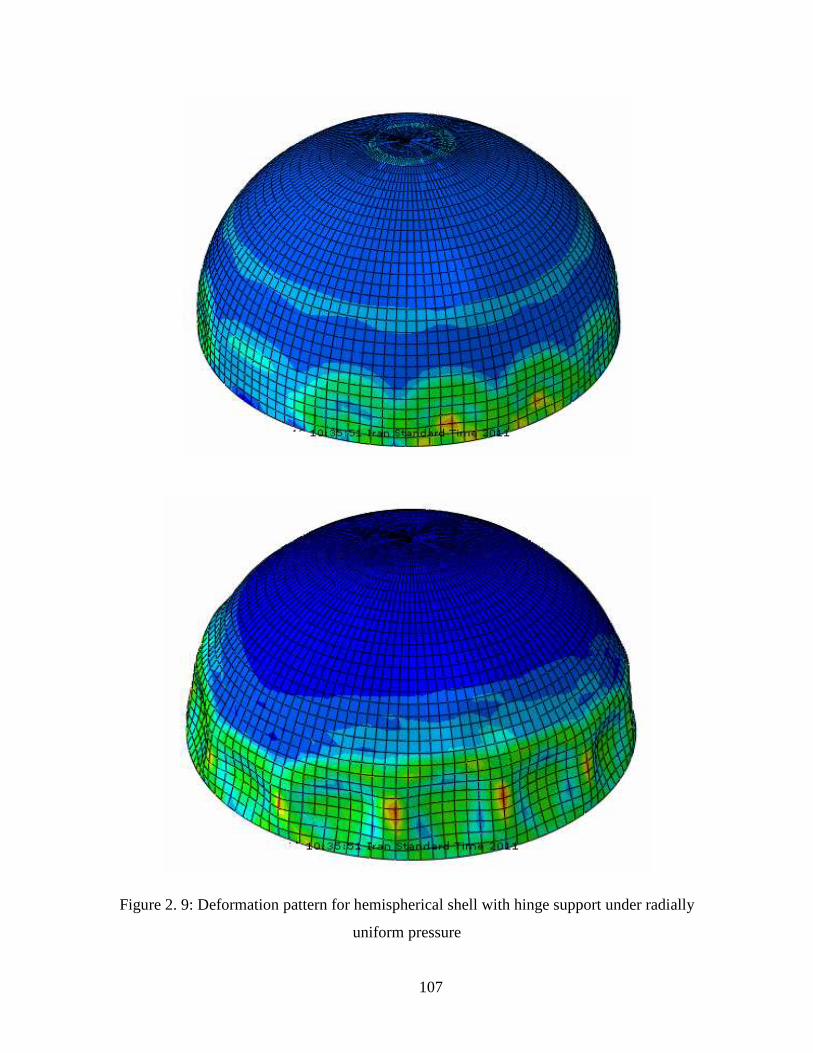
107
Figure 2. 9: Deformation pattern for hemispherical shell with hinge support under radially
uniform pressure

108
Figure 2. 10: Subsequent deformation of hemispherical shell with hinge support under radially
uniform pressure

109
Figure 2. 11: Deformation of hemispherical shell with hinge support under maximum radially
uniform pressure

110
Figure 2. 12: Different cuts of the deformed hemispherical shell with hinge support under
radially uniform pressure

111
Figure 2. 13: Subsequent deformations in the cuts of the deformed hemispherical shell with
hinge support under radially uniform pressure

112
Figure 2. 14: Buckling initiation of the hemispherical shell with roller support under radially
uniform pressure

113
Figure 2. 15: Subsequent deformation of the hemispherical shell with roller support under
radially uniform pressure

114
Figure 2. 16: Second mode of the deformation in hemispherical shell with roller support under
radially uniform pressure

115
Figure 2. 17: Buckling initiation of the hemispherical shell with hinge support under ring load in
2R

116
Figure 2. 18: Buckling of the hemispherical shell with hinge support under ring load at 2R
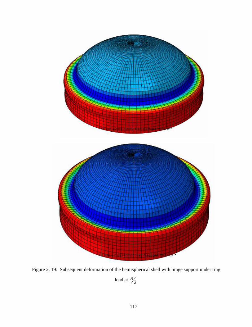
117
Figure 2. 19: Subsequent deformation of the hemispherical shell with hinge support under ring
load at 2R
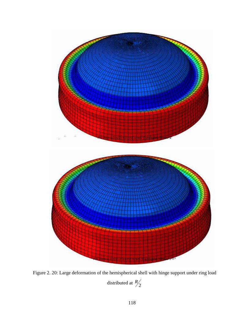
118
Figure 2. 20: Large deformation of the hemispherical shell with hinge support under ring load
distributed at 2R

119
Figure 2. 21: Buckling initiation of the hemispherical shell with hinge support under ring load in
3R

120
Figure 2. 22: Buckling of the hemispherical shell with hinge support under ring load at 2R

121
Figure 2. 23: Large deformation of the hemispherical shell with hinge support under ring load
distributed at 3R
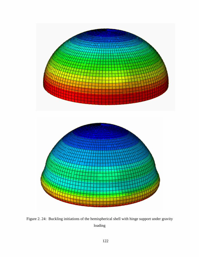
122
Figure 2. 24: Buckling initiations of the hemispherical shell with hinge support under gravity
loading

123
Figure 2. 25: Subsequent deformation of the hemispherical shell with hinge support under
gravity loading

124
2.7. Experimental Program
In this part, an attempt is made to find the critical load for hemispherical shells pinned at
the base and subject to uniform pressure in a purely experimental way. It is intended to show
that the formulation which has been derived in this study give correct results for shells of
revolution under various axisymmetric loading conditions.
A total of six thin walled polyethylene hemispherical shells were constructed and tested under
uniform suction pressure. The base diameters of these shells were 15 cm and 10 cm and their
wall thickness were 0.05 cm yielding tR ratios of 150 and 100 respectively. It is evident that
the construction of these shells through machining would have been difficult and for the
following reasons, the shells were made of solid polyethylene plastic which posses good tensile,
flexural, and impact strengths and its flexural modulus is proportional to the stiffness of the
material. Its creep resistance is excellent and is substantially superior to most plastics. Its
mechanical properties are as follows:
Flexural modulus: 650 MPa
Poisson’s ratio: 0.4
Density: 1150 kg/m3
Poisson’s ratio: 0.4
A complete family of hemispherical shells is shown in Fig 2.26.
The manufacturing of these shells was carried out with the aid of machined male and
female molds made from cast aluminum alloy. The aluminum alloy molds were machined with
considerable precision and then the spherical shells were cast by “puddling” technique. Each
shell was inspected by a polariscope to ensure that no air bubbles were trapped in the shell wall.
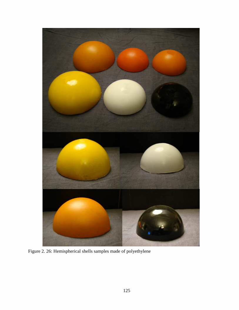
125
Figure 2. 26: Hemispherical shells samples made of polyethylene

126
Figure 2. 27: A test made of R=75 mm shell using suction pressure and three displacement
gages at various points.
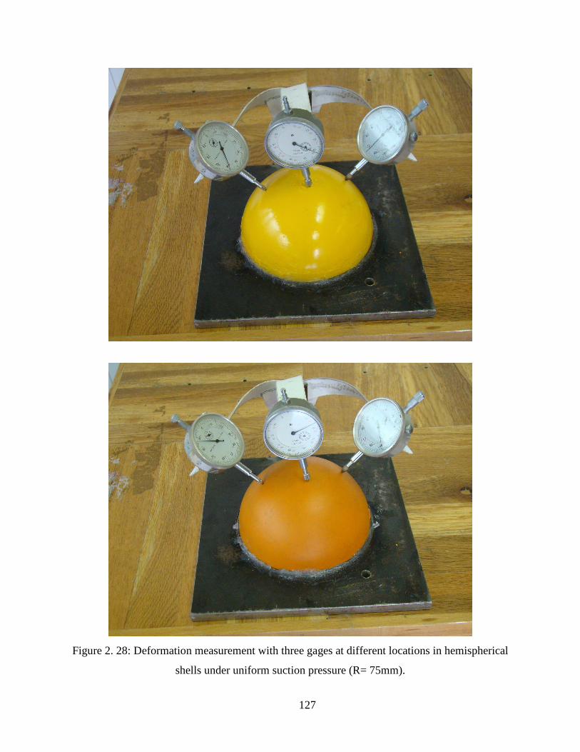
127
Figure 2. 28: Deformation measurement with three gages at different locations in hemispherical
shells under uniform suction pressure (R= 75mm).
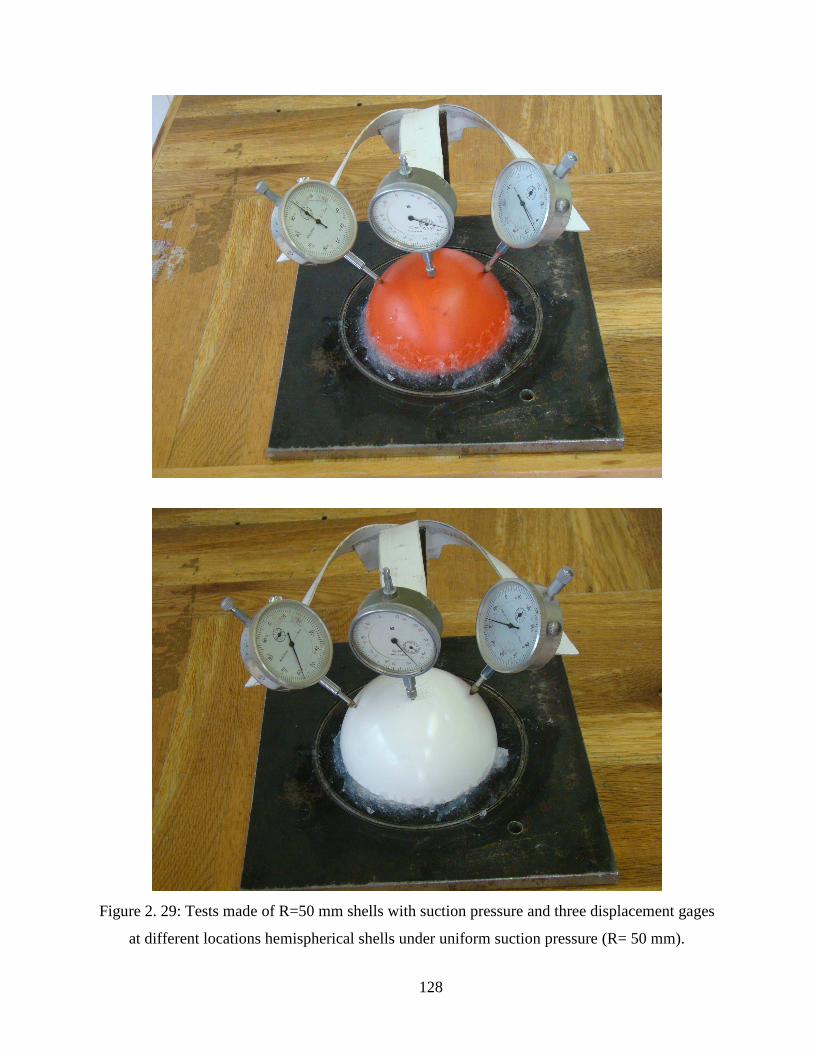
128
Figure 2. 29: Tests made of R=50 mm shells with suction pressure and three displacement gages
at different locations hemispherical shells under uniform suction pressure (R= 50 mm).
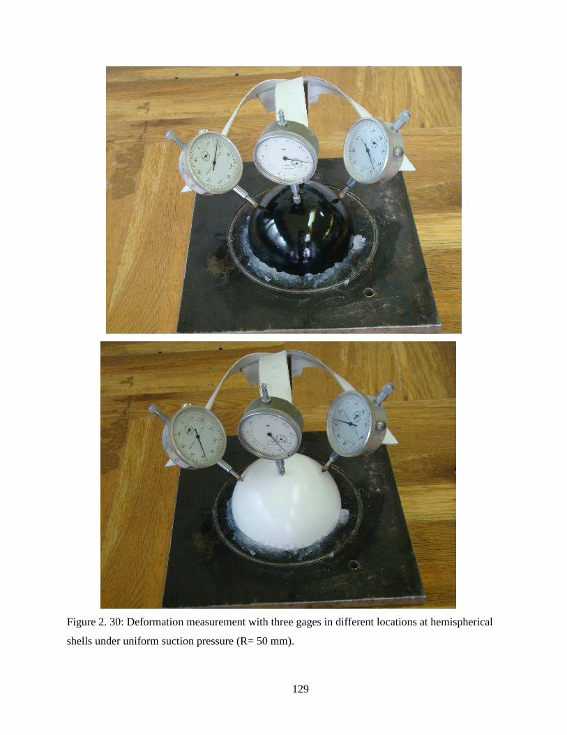
129
Figure 2. 30: Deformation measurement with three gages in different locations at hemispherical
shells under uniform suction pressure (R= 50 mm).

130
Figure 2. 31: Initial buckling of hemispherical shells under uniform suction pressure (R= 50
mm).
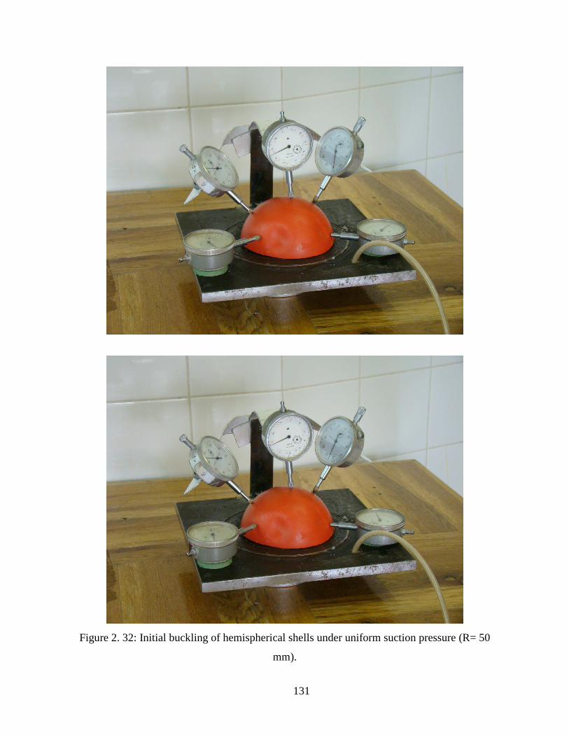
131
Figure 2. 32: Initial buckling of hemispherical shells under uniform suction pressure (R= 50
mm).
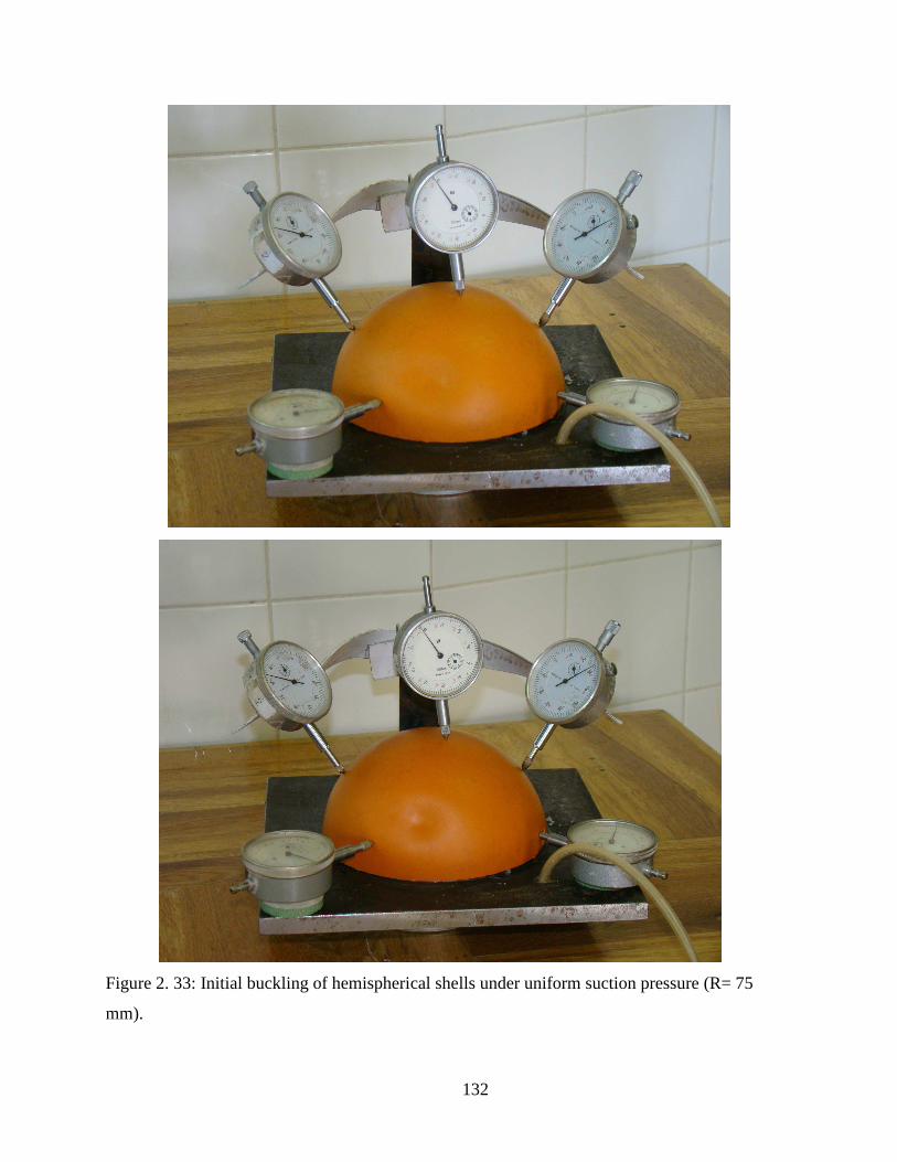
132
Figure 2. 33: Initial buckling of hemispherical shells under uniform suction pressure (R= 75
mm).

133
Figure 2. 34: Several tests made on different samples using suction pressure with three and five
gages at different locations.

134
2.8. Results and Discussion
In this study, the Southwell predictions are compared with experimentally, and
numerically obtained values. The results of the investigation are summarized in Figs 2.35 to 2.45
which the predictions of the Southwell method are compared with measured buckling loads in
experimental study and numerical simulations. Scatter in the experimentally obtained buckling
pressures is probably due to variations that existed occurred in the specimens because of the fact
that each one was cast separately. The manufacturers did, however, take considerable care during
the manufacturing process, and especially with the mix, and for this reason the scatter is very
small. Thus, it is likely that the main source of error compared to theory is because of
measurement reading errors, and imperfections in material properties. However, the agreement
between measured buckling load and Southwell prediction is remarkable. Mostly, the Southwell
method tended to yield buckling loads which are slightly higher than those measured and the
disparity of buckling load is somewhat difficult to detect. Nevertheless, the predicted loads are
reliable to be slightly higher (up to about 17%) than the actual load encountered. Therefore, a
reasonable degree of caution is recommended to be exercised.Scatter in the numerically obtained
buckling pressures for axisymmetrical buckling cases are very small and it is most likely due to
the assumptions of the finite element solution. For the case of buckling of spherical shell with
roller support under uniform pressure, the buckled shape is not axisymmetric anymore (Fig
2.15). So, once data are collected from the principle axes locations, the answer is acceptable and
there is only 13% error otherwise, the deviation from the correct values is considerable.
Briefly, the method provides valuable technique for estimating the buckling load of
spherical shells without having to conduct a destructive test. The results obtained have logical
accuracy and the method does not suffer from the any major issues. Any boundary condition at

135
the edge may be taken into account and as long as the loading is axisymmetric, this procedure
can be used with reasonable accuracy.
2.8.1 Experimental work findings
w/p-w
y = -0.1321x + 3.1309
3.11
3.112
3.114
3.116
3.118
3.12
3.122
3.124
3.126
3.128
3.13
0 0.05 0.1 0.15
w (mm)
w/p
(m
m3 /
N)
Experimental
Figure 2. 35: Plot of pw against w ( mmR 50= , mmt 5.00 = )
1321.0−=S
( ) MPapS
Emp crcr 088.0
13
42
32 =→
−−=
υ
From test MPap 078.0=
Error for this case: %8.12100078.0
078.0088.0 =×−

136
w/p-w
y = -0.135x + 3.1372
3.1
3.105
3.11
3.115
3.12
3.125
3.13
3.135
0 0.05 0.1 0.15 0.2 0.25 0.3
w (mm)
w/p
(m
m3 /
N)
Experimental Numerical
Figure 2. 36: Plot of pw against w ( mmR 50= , mmt 5.00 = )
135.0−=S
( ) MPapS
Emp crcr 087.0
13
42
32 =→
−−=
υ
From test MPap 078.0=
Error for this case: %15.10100078.0
078.0087.0 =×−

137
w/p-w
y = -0.1179x + 3.2099
3.199
3.2
3.201
3.202
3.203
3.204
3.205
3.206
3.207
3.208
3.209
3.21
0 0.02 0.04 0.06 0.08 0.1
w (mm)
w/p
(m
m3 /
N)
Experimental
Figure 2. 37: Plot of pw against w ( mmR 50= , mmt 5.00 = )
1179.0−=S
( ) MPapS
Emp crcr 0935.0
13
42
32 =→
−−=
υ
From test MPap 08.0=
Error for this case: %8.1610008.0
08.00935.0 =×−

138
w/p-w
y = -0.1885x + 5.5705
5.55
5.552
5.554
5.556
5.558
5.56
5.562
5.564
5.566
5.568
5.57
0 0.02 0.04 0.06 0.08 0.1 0.12
w (mm)
w/p
(m
m3 /
N)
Experimental
Figure 2. 38: Plot of pw against w ( mmR 75= , mmt 5.00 = )
1885.0−=S
( ) MPapS
Emp crcr 040.0
13
42
32 =→
−−=
υ
From test MPap 035.0=
Error for this case: %28.14100035.0
035.0040.0 =×−

139
w/p-w
y = -0.183x + 5.0223
5.002
5.004
5.006
5.008
5.01
5.012
5.014
5.016
5.018
5.02
5.022
0 0.02 0.04 0.06 0.08 0.1 0.12
w (mm)
w/p
(m
m3 /
N)
Experimental
Figure 2. 39 : Plot of pw against w ( mmR 75= , mmt 5.00 = )
183.0−=S
( ) MPapS
Emp crcr 0408.0
13
42
32 =→
−−=
υ
From test MPap 035.0=
Error for this case: %5.16100035.0
035.00408.0 =×−
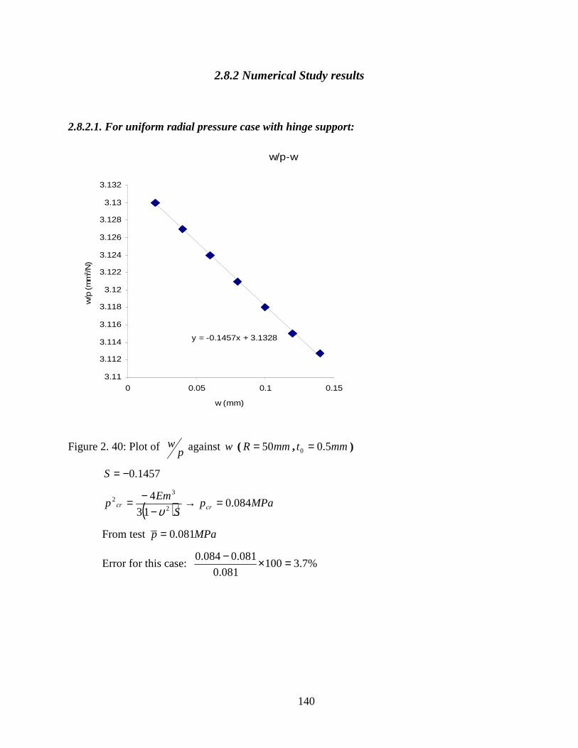
140
2.8.2 Numerical Study results
2.8.2.1. For uniform radial pressure case with hinge support:
w/p-w
y = -0.1457x + 3.1328
3.11
3.112
3.114
3.116
3.118
3.12
3.122
3.124
3.126
3.128
3.13
3.132
0 0.05 0.1 0.15
w (mm)
w/p
(m
m3 /
N)
Figure 2. 40: Plot of pw against w ( mmR 50= , mmt 5.00 = )
1457.0−=S
( ) MPapS
Emp crcr 084.0
13
42
32 =→
−−=
υ
From test MPap 081.0=
Error for this case: %7.3100081.0
081.0084.0 =×−

141
w/p-w
y = -0.2004x + 5.571
5.55
5.552
5.554
5.556
5.558
5.56
5.562
5.564
5.566
5.568
5.57
0 0.02 0.04 0.06 0.08 0.1 0.12
w (mm)
w/p
(m
m3 /
N)
Figure 2. 41: Plot of p against w ( mmR 75= , mmt 5.00 = )
2.0−=S
( ) MPapS
Emp crcr 039.0
13
42
32 =→
−−=
υ
From test MPap 037.0=
Error for this case: %4.5100037.0
037.0039.0 =×−

142
2.8.2.2. For uniform downward pressure case with hinge support:
w/p-w
y = -1.9107x + 9.6
9.3
9.35
9.4
9.45
9.5
9.55
9.6
0 0.05 0.1 0.15
w (mm)
w/p
(m
m3 /
N)
Figure 2. 42: Plot of pw against w ( mmR 50= , mmt 5.00 = )
9107.1−=S
Buckling pressure using Southwell method ( ) MPapS
Emp crcr 023.0
13
42
32 =→
−−=
υ
Buckling pressure MPap 022.0=
Error for this case: %5.4100022.0
022.0023.0 =×−

143
2.8.2.3. For uniform radial pressure case with roller support :
w/p-w
y = -51.014x + 135.17
114
116
118
120
122
124
126
128
130
132
134
0 0.1 0.2 0.3 0.4
w (mm)
w/p
(m
m3 /
N)
Figure 2. 43: Plot of pw against w ( mmR 50= , mmt 5.00 = )
014.51−=S
Buckling pressure using Southwell method ( ) MPapS
Emp crcr 0039.0
13
42
32 =→
−−=
υ
Buckling pressure MPap 0044.0=
Error for this case: %2.131000039.0
039.00044.0 =×−

144
2.8.2.4. For Ring load case with hinge support:
w/p-w
y = -7.8929x + 13.261
12
12.2
12.4
12.6
12.8
13
13.2
0 0.05 0.1 0.15
w (mm)
w/p
(m
m3 /
N)
Figure 2. 44: Plot of pw against w ( mmR 50= , mmt 5.00 = )
8929.7−=S
Buckling pressure using Southwell method
( ) mmNqMPapS
Emp crcr /57.00114.0
13
42
32 =→=→
−−=
υ
Buckling pressure MPap 5.0=
Error for this case: %1410050.0
50.057.0 =×−
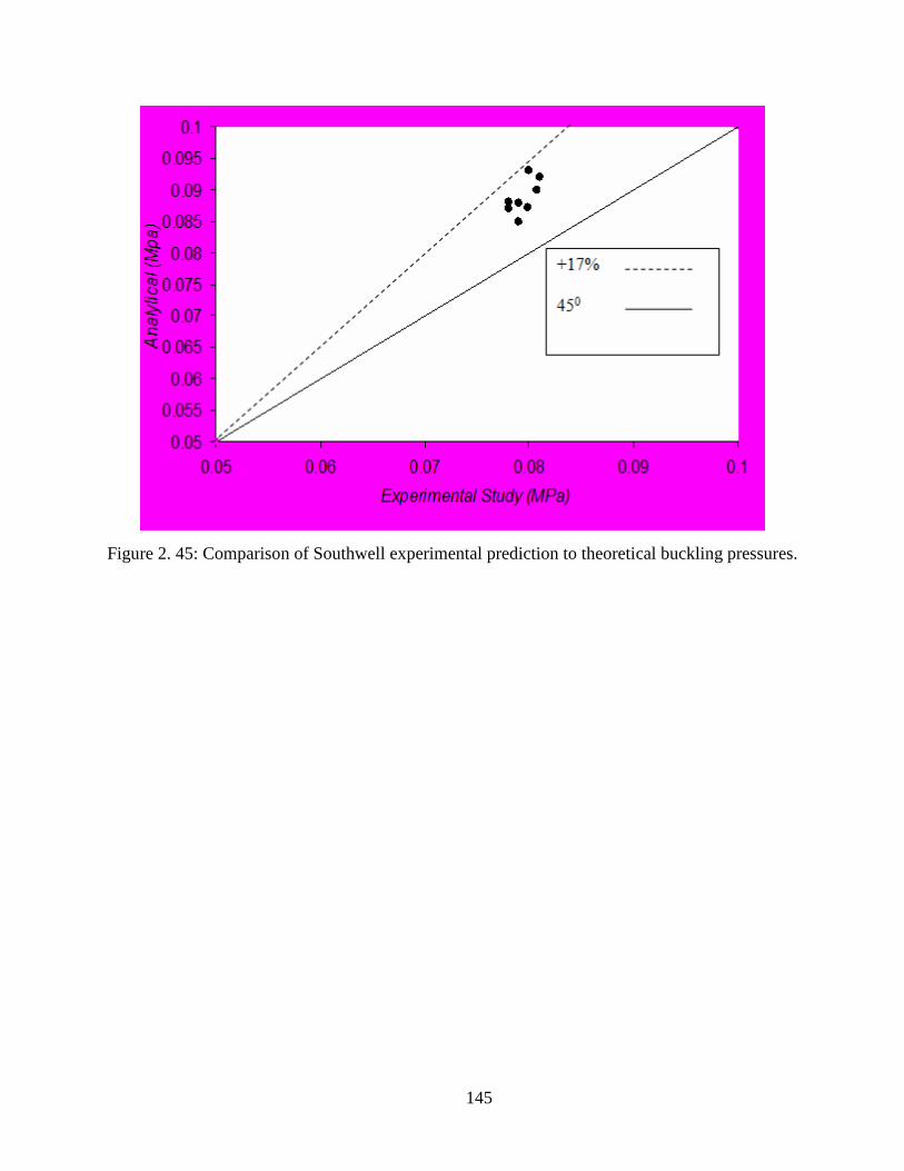
145
Figure 2. 45: Comparison of Southwell experimental prediction to theoretical buckling pressures.
146
2.9. Conclusion
The accurate prediction of buckling loads of spherical shells, based on the nondestructive
buckling test data, is generally a difficult problem. Hence, this chapter presents a general
methodology for predicting the critical buckling loads of spherical shells using a nondestructive
test. For this purpose, the well known graphical method of predicting buckling loads, i.e., the
Southwell’s nondestructive method is extended to spherical shells and a new formula is derived
for the critical buckling load of uniformly compressed spherical shells. The feasibility of this
technique for determining critical buckling loads of spherical shells is demonstrated provided
caution is exercised in analyzing the test results. This method may be used in any kind of
spherical shells with arbitrary axisymmetrical loading and it provides a valuable procedure for
estimating the buckling load of a spherical shell structure without having to conduct a destructive
test. In this method, the curve of displacement/load is plotted against displacement, which is a
straight line, and the slope of this line when multiplied by a constant value presents the critical
buckling load with sufficient accuracy. The expediency of the method lies in its simplicity, and
in the fact that it is nondestructive. This technique does not need any assumption as to the
number of buckling waves or the exact locality of buckling so long as the loading remains
axisymmetric. During experimental study, the test can be terminated if enough data points have
formed a straight line. In this procedure, error may be introduced as a result of the accuracy of
instruments, skill of the examiner and also approximation in determining Poisson’s ratio value.
Moreover, the accuracy of this method depends on the test cut off point and the mathematical
function which is used for curve fitting. In the least squares fitting technique, the slope of the

147
fitted line is affected by the accuracy of the different displacement data points. Small
inaccuracies in the measured data points cause the slope of line to be changed noticeably and
may cause over prediction of the buckling load. So, with increasing the number of data points
plotted together one can get more precise and realistic buckling load. The data points in the
lower region are less important than the data points in the higher load region. In addition,
increasing the number of gages may tremendously improve the accuracy. Even though the
numerical solution can make the buckling load easily available to the user, it is here as an
additional tool to verify the accuracy of the Southwell technique compared with the actual
numerical and analytical buckling loads. Excellent correlation is observed.

148
Notation that used in this chapter
SSlope of w verses pw line
u Displacement of the shell element in x direction
v Displacement of the shell element iny direction
w Displacement of the shell element inz direction
0U Effect of initial imperfections
V Shearing force in straight members
y Deflection of straight member
α Buckling coefficient to be determined experimentally
xε The unit elongation or strain in x- direction
yε The unit elongation or strain in y-direction
1ε The unit elongation of middle surface in x-direction
2ε The unit elongation of middle surface in y-direction
υ Poisson’s ratio
xχ Change of curvature in x-direction
yχ Change of curvature in y-direction
0t Thickness of shell
crp Classical buckling pressure
( )H A mathematical operator

149
References
Abramovich, H., Weller, T. and Yaffe, R. (1990). “Application of a Modified Southwell
technique for the determination of critical loads of imperfect plates”, Computers and Structures,
Volume 37, Issue 4, pp.463-469.
Archer, R.R. and Lange, C.G. (1965). “On the Nonlinear Dynamic Behavior of Shallow
Spherical Shells”, AIAA Journal. Vol.3. pp. 2313-2317.
Archer, R.R. and Famili, J., (1965). “On the Vibrations and Stability of Finitely
Deformed Shallow Spherical Shells”, J. App. Mech. Vol. 32. pp.116-120.
Beyer, K. (1933-1934). “Die Statik im Eisenbetonbau : ein Lehr-und Handbuch der
Baustatik”, vol.2 Berlin: Julius Springer.
Bhimaraddi A., Carr J., and Moss P.J., (1989). “A Shear Deformable Finite Element for
the Analysis of General Shells of Revolution”, Computer and Structures, Vol.31, (3), pp.299-
308.
Bleich, F., (1952).“Buckling Strength of Metal Structures”, McGraw-Hill, 256p.
Bowles, R. E., and Merchant, W., (1956). “Critical Loads of Tall Building Frames” The
Structural Engineer,Vol 36, Pp. 324-329.
Brush, D. O., Almroth, B. O., (1975). “Buckling of bars, plates and shells”, New York:
McGraw-Hill Books Company, 325p.
Budiansky, B. and Hutchinson, J. W. (1964). “Dynamic Buckling if Imperfection
Sensitive Structures”, Proceeding of the XI International Congress of Applied Mechanics, edited
by Gortler, H., Springer-Verlag, Berlin, pp.639-651.

150
Budiansky, B., (1959). “Buckling of Clamped Shallow Spherical Shells” Proceeding of
the symposium on the Theory of thin Elastic Shells, Delft, North Holland Publishing Company,
Amsterdam, pp.64-94.
Budiansky, B., (1966). “Dynamic Buckling of Elastic Structures: Criteria and Estimate.”
Proceedings, International Conference on Dynamic Stability of Structures. Pergamon, New
York, pp.83-106.
Budiansky, B., and Roth, R., (1962). “Axisymmetric Dynamic Buckling of Clamped
Shallow Spherical Shells”. NASA TN D-1510, pp.597-609.
Chan H.C., (1989). “Geometrically Nonlinear Analysis of Shallow Shells using Higher
Order Finite Elements”, Compure Structure, Vol. 31, No.3, pp.329-338.
Choi C., Yoo S., (1991). “Geometrically Nonlinear Behavior of an Improved
Degenerated Shell Element”, Compure Structure Vol.40, No.3, pp.785-794.
Cohen, G. A. (1968). “Effect of a Nonlinear Prebuckling State on the Postbuckling
Behavior and Imperfection Sensitivity of Elastic Structures”, AIAA Journal, Vol.6. No.8.
pp.1616-1619.
Del Pozo, F, (1973). “La cúpula del Palau Blau-Grana”, Hormigón y Acero, 107-108, pp.
Delpak R., and Peshkam V., (1991). “A Variational Approach to Geometrically
Nonlinear Analysis of Asymmetrically Loaded Rotational Shells: Theory and Formulation”,
Computer Structure, Vol.39, No.34, pp.317-326.
Drucker, D. C., Greemberg, W., and Prager, W. (1951).‘The safety factor of an elastic
plastic body in plane strain’, Trans. A.S.M.E., Journal of Appied Mechanic, Vol. 173, No.1
p.371.
151
Drucker, D.C., and Shield, R.T., (1959). “Limit Analysis of Symmetrically Loaded Thin
Shells of Revolution” Journal of Applied Mechanics, Vol. 26, pp 61-68.
Dumir, P. C. , Gandhi, M. L., and Nath, Y., (1984). “Axisymmetric static and dynamic
buckling of orthotropic shallow spherical cap with circular hole ” Computers and Structures,
Volume 19, No.5, Pages 725-736.
Dumir, P. C., Dube, G. P., and Mallick, A., (2005). “Axisymmetric buckling of laminated
thick annular spherical cap ” Communications in Nonlinear Science and Numerical Simulation,
Vol. 10, Issue 2, pp191-204.
Eller C., (1990) “Finite Element Procedures for the Stability Analysis of Nonlinear
Parametric Excited Shell Structures”, Computer and Structure Vol.35, No.3, pp.259-265.
Euler, Leonhard, (1744). “De Curvis Elasticis” Lausanne-Genf, Switerland, pp.72-160.
Famili, J. and Archer, R. R. (1965). “Finite Asymmetric Deformation of Shallow
Spherical Shells”, AIAA Journal, Vol.3, pp. 506-510.
Famili, J. (1965) “Asymmetric Buckling of Finitely Deformed Conical Shells”, AIAA
Journal, Vol.3, No.8, pp.1456-1461.
Fauconnier, (1934). “Essai de rupture d' una voûte mince conoïde en béton armé”,
Proceedings IABSE, Vol. II, pp. 167-192.
Fitch, J.R., and Budiansky, B., (1970). “Buckling and Postbuckling Behavior of Spherical
Caps under Axisymmetric Load”, AIAA Journal. Vol.8, No.4, pp.686-693.
Flügge, W, (1934). “Statik und dynamik der schalen”, Berlin: Julius Springer, 118p.
Flügge, W, (1960). “Statique et dynamique des coques”, Paris: éditions eyrolles.
Flügge, W, (1960). “Stresses in Shells”, Springer-Verlag, Berlin.

152
Föppl, A, (1930). “Résistance des matériaux et éléments de la théorie mathématique de
l'élasticité”, Paris, Gauthier-Villars et Cie.
Foster, G.C, Tennyson, R.C. (1983). “Use of the Southwell Method to Predict Buckling
Strengths of Stringer Stiffened Cylindrical Shells”, An International Journal for Experimental
Mechanics, Volume 19, Issue 2, pp.63-67.
Fung, Y. C. (1974). “Thin Shell Structures: Theory, Experiment and Design”, Prentice
Hall, USA, pp. 247-259.
Gill S.S., and Leckie F.A., (1968).“The Effect of Geometry Change on The Application
of Limit Analysis to the Design of Pressure Vessel Nozzles” International Journal of Mechcal
Science, Vol 10, pp.989-993.
Goncalves, P. B. and Croll, J. G. S. A. (1992). “ Axisymmetric Buckling of Pressure
Loaded Spherical Caps”, Journal of Structural Engineering, Vol. 118, No.4, pp. 970-985.
Grafton P.E., Strome D.R., (1963). “Analysis of axisymmetric Shells by the Direct
Stiffness Method”, AIAA Journal, Vol.2, No.3, pp 304-332.
Gregory, M.S., (1968). “Elastic Instability”, Spon Ltd.
Grünitz, L., (2003).“The effect of welding on the buckling behavior of a spherical cap”
International Journal of Pressure Vessels and Piping, Vol. 80, Issue 4, pp. 237-241.
Gupta P.K., Gupta N.K., (2009). “A Study of Axial Compression of Metallic
Hemispherical Domes” Journal of Materials Processing Technology, Vol. 209, Issue 4, pp.2175-
2179.
Hetenyi. M, (1950). “Handbook of Experimental Stress Analysis” John Wiley and Sons.
Hodge, P. G., (1965). “Limit Analysis of Rotationally Symmetric Plates and Shells”
Prentice-Hall Inc., Englewood Cliffs, N.J.

153
Hsiao K., Chen Y., (1989).“Nonlinear Analysis of Shell Structures by Degenerated
Isoparametric Shell Element”, Computer and Structure Vol.31, No.3, pp.427-438.
Huang N.C., (1964). “Unsymmetric Buckling of Thin Shallow Spherical Shells”,
Tranaction of ASME, Journal of Applied Mechanics, Vol.32, pp.447-457.
Huang N. C., (1969). “Axisymmetric Dynamic Snap-through of Elastic Clamped Shallow
Spherical Shells”, AIAA Journal Vol.7, No.2, pp215-220.
Humphreys, J. S. and Bodner, S. R., (1962). “Dynamic Buckling of Shallow Shells under
Impulsive Loading”, Journal of Engineering Mechanics,ASCE, Proceedings of the American
Society of Civil Engineers Journal of the Engineering Mechanics Division 88 (1962), pp. 17–36.
Hutchinson, J. W. (1967). “Imperfection Sensitivity of Externally Pressurized Spherical
Shells”, Transaction of ASME, Journal of Applied Mechanics, Vol. 34, No 49, pp.49-55.
Ingerslev A., (1923). “The Strength of Rectangular Slabs”, The Institution of Structural
Engineers Journal. Vol.1, No.1, pp.3-14.
Jones L.L., (1962). “ Ultimate Load Analysis of Reinforced and Prestressed Concrete
Structures”, Chatto and Windus, London, 248p.
Jones L.L., and Wood R.H., (1967). “Yield Line Analysis of Slabs”, Thames and
Hudson, London, 405p.
Jones, G. W. and Chapman, S. J. and Allwright, D. J. (2008). “Axisymmetric buckling of
a spherical shell embedded in an elastic medium under uniaxial stress at infinity,” The Quarterly
Journal of Mechanics and Applied Mathematics, Vol. 61, No.4, pp. 475-495.
Kaplan, A. and Fung, Y. C. (1954). “A Nonlinear Theory of Bending and Buckling of
Thin Elastic Shallow Spherical Shells” NACA TN 3212, 17p.

154
Koiter, W. T. (1945).“On the Stability of Elastic Equilibrium”, Thesis, Delft, H.J. Paris
Amsterdam.
Koiter, W.T. (1963). “Elastic Stability and Post Buckling behavior”, Proceedings of
Symosium on Nonlinear Problems, edited by Langer R. E., University of Wisconsin Press, p.257.
Liang C.C., Liao C.C. and Ma Y.C., (1991). “A large Deformation Elastic Plastic
Dynamic Analysis of Square Plate and Spherical Shell Subjected to Shock Loading” Computer
and Structure, Vol.39, No.6, pp 653-661.
Luo, P., Luo, H., Tong, F., (1991). “The Influence of Pre buckling Deformations and
Stresses on the Buckling of the Spherical Shell”, International Journal of Offshore and Polar
Engineering, Vol.1, No.4, pp 25-37.
American Institute of Steel Construction (AISC), (2008). “Manual of Steel
Construction”.
Nagtegaal, J.C., Parks, D.M., and Rice, J.R. (1974). “On Numerically Accurate Finite
Element Solutions in the Fully Plastic Range” Computers Methods in Applied Mechanics and
Engineering, Vol. 4, No., pp 153-177.
Nie, G. H., Chan, C. K., Yao, J. C., and He, X. Q. (2009).“Asymptotic Solution for
Nonlinear Buckling of Orthotropic Shells on Elastic Foundation,” AIAA Journal, vol. 47, No.7,
pp. 1772-1783.
Palassopoulos, G. V. (1992). “Response Variability of Structures Subjected to
Bifurcation Buckling”, Journal of Engineering Mechanics, ASCE, Vol.118, EM6 proceedings,
pp. 1164-1183.
Roorda, J.,(1967). “Some Thoughts on the Southwell Plot” Journal of Engineering
Mechanics Division, ASCE, Vol 93, (EM6) proceedings, Paper 5634, pp.37-48.

155
Seide, P. (1975). “Small Elastic Deformations of Thin Shells”, Noordhoff International
Publishing Leyden, California, USA, pp.227-229.
Seide, P., (1962). “On the Stability of Internally Pressurized Conical Shells under Axial
Compression”, Proceedings of the Fourth U.S. National Congress of Applied Mechanics, Vol.2
pp.761-773.
Singer, J. (1961). “Buckling of Conical Shells under Axisymmetrical External Pressure”,
Journal of Mechanical Engineering Science, Vol.3. No.4. p.330.
Singer, J., Eckstein A., Baruch. M, (1962). “Buckling of Conical Shells under External
Pressure, Torsion and Axial Compression”, TAE Report No.19. Technion Research and
Development Foundation, pp.97-122.
Southwell, R. V., (1932). “On the Analysis of Experimental Observations in Problems of
Elastic Stability” Proceedings of Royal Society of London (A), Vol.135, pp.601-616.
Stephens, W. B., and Fulton, R. E. (1969). “Axisymmetric Static and Dynamic Buckling
of Spherical Caps due to Centrally Distributed Pressures”, AIAA Journal, Vol.7, No.11, p.2120.
Stricklin, J.A., Martinez, J.R., Tillerson, J.R., Hong, J. H., and Haisler, W.E., (1971).
“Nonlinear Dynamic Analysis of Shells of Revolution by Matrix Displacement Method”, AIAA
Journal Vol.9, No.4, pp629-636.
Stricklin, J.A., and Martinez, J.E., (1969). “Dynamic Buckling of Clamped Spherical
Caps under Step Pressure Loading”, AIAA Journal Vol.7 No.6, pp.1212-1213.
Teng J.G., and Rotter J.M., (1989).“Elastic-Plastic large Deflection Analysis of
Axisymmetric Shells”, Computer and Structure, Vol.31, No.2, pp.211-233.
Terndrup, P., Jensen, J., (1995). “Buckling Behavior of Imperfect Spherical Shells
Subjected to Different Load Conditions”, Thin-Walled Structures, Vol.23, No.4, pp.41-45.

156
Thurston, G. A. (1961) “A numerical Solution of The Nonlinear Equations for
Axisymmetric Bending of Shallow Spherical Shells”, Transactions of ASME, Journal of Applied
Mechanics, pp. 557-562.
Thurston, G. A. ,Penning, F. A. (1966). “Effect of Axisymmetric Imperfections on the
Buckling of Spherical Caps under Uniform Pressure”, AIAA Journal, Vol.4, No.2, pp.319-327.
Tillman, S. C. (1970). “On the Buckling Behavior of Shallow Spherical Caps under
Unifor Pressure Load”, International Journal of Solids Structures, Vol.6, pp.37-52.
Timoshenko, S., (1953). “History of Strength of Materials” Mc-Graw-Hill.
Timoshenko, S., and Gere (1961). “Theory of elastic Stability” Mc-Graw-Hill Second Ed.
Timoshenko, S., and Krieger (1959). “Theory of Plate and Shells” Mc-Graw-Hill Second
Ed.
To C.W., and Wang B., (1991).“An Axisymmetric Thin Shell Finite Element for
Vibration Analysis”, Computers and Structures, Vol.40, No.3, pp.555-568.
Torroja, E., (1934). “Cubiertas laminares de hormigón armado”, Madrid: Instituto
Técnico de la Construcción u Edificación, 315p.
Uchiyama, M. and Yamada, S. (2003). “Nonlinear Buckling Simulations of Imperfect
Shell Domes by Mixed Finite Elements” Journal of Engineering Mechanics,ASCE, Vol.
129,No.7, pp. 707-714.
Von Karman, T. (1909). “Untersuchungen uber Knickfestigkeit” Ver, Deust, Ing, Berlin.
Von Karman, T., and Tsien, H. S., (1939). “The Buckling of Spherical Shells by
External Pressure” Journal of Aerospace Science, Vol.7, No.2, p.43.
Weinitschke, H. (1960) “On the Stability Problem for Shallow Spherical Shells”, Journal
of Mathematics and Physics. Vol.38, No.4, p. 209.

157
Winter, G., Hsu, P.T., Koo, B., and Loh, M.H. (1948).“Buckling of Trusses and Rigid
Frames”, Cornell University, Engineering Experiment Station Bulletin, No. 36.
Xie C.R., and Ho D., (1990). “Axisymmetric Buckling of Truncated Shallow Spherical
Shells”, Computers and Structures, Vol.34, No.2, pp.297-301.
Xu C.S., (1991). “Buckling and Post-Buckling of symmetrically laminated moderately-
thick spherical caps” International Journal of Solids and Structures, Vol. 28, No. pp1171-1184.
Yiniyi, Z. (1999). “Torsional Buckling of Spherical Shells under Circumferential Shear
Loads”, Applied Mathematics and Mechanics, Vol.20, No.4.
Yuan K.Y. and Liang C.C.,(1989). “Nonlinear Analysis of an Axisymmetrc Shell using
Three Noded Degenerated Isoparametric Shell Element”, Computers and Structures, Vol.32,
No.6, pp.1225-1239.
Zheng X., and Zhou Y., (1989). “Analytical Computerization Method for Solving a Kind
of Nonlinear Equation of Plate and Shells”, Computers and Structures Vol.32, No.1, pp.185-194.
Zweig, A., (1968).“Buckling Analysis of One Story Frames”, Journal of the Structural
Division, ASCE 94, ST9 , pp. 2107–2134
158
Appendix A - Collapse load of circular plate
A plate is supposed to yield in bending at point ( )21, xx if the stress tensor there obeys the
yield criterion at every 3x except 03 =x ; points in the middle plane are observed as remnants of
the elastic core. If the stresses 3iσ are assumed negligible in magnitude next to the αβσ (this does
not mean that they can be neglected in the equilibrium equations, because derivatives occur
there), then a plane-stress yield criterion may apply:
,0=
y
fσσ αβ
In every plane 03 ≠x . Equilibrium is satisfied if
32sgn
4xM
hαβαβσ −=
If the ultimate moment is defined as ,4
20
0
tM yσ= then the plate yield criterion is given
by ( ) ,0=αβmf
where ;0M
Mm αβ
αβ = the Mises and Tresca criteria become, respectively,
13 212
2222211
211 =++− mmmmm (Mises),
( ) 1,,max 2121 =− mmmm (Tresca),
If the loading and support are axisymmetric, then the only nonvanishing moments
are rM , θM and the equilibrium equation is,
159
( ) ∫=−′ r
r qrdrMrM0θ (A.1)
This equation and the yield condition constitute two equations for rM and θM .
Equivalently, if the yield condition is solved for θM in terms of rM and the resulting expression
for θM is substituted in (A.1), the result is a nonlinear first order differential equation for rM . At
the center of the plate, θMM r = and thus, if the curvature there is positive (concave upward),
( ) 00 MM r = constitutes an initial condition with which the differential equation may be solved.
In addition, a boundary condition at the edge ar = must be satisfied; this yields the ultimate
load. Let us recall that for a simply supported plate, the edge conditions are 0== rMw thus
0=rM is a boundary condition with which the differential equation may be solved. For a
clamped plate, the edge must form a hinge circle, that is, a locus of slope discontinuity. As we
shall see, the edge condition there becomes ( ) 0MaM r = or ( )3
2 0MaM r−= for the Tresca
or Mises material, respectively. Fig A.1 shows the Mises and Tresca yield criteria for
axisymmetrically loaded circular plates. It follows from the preceding discussion that the center
of the plate is in the moment state corresponding to point B, and that a simply supported edge
corresponds to point C. A simply supported plate may thus be assumed to be entirely in the
regime BC. For the the Tresca material, this means that 0MM =θ everywhere, and the problem
to be solved is therefore linear.

160
Figure A. 1: Mises and Tresca yield criteria for axisymmetrically loaded circular plates
Solution for Tresca Plate
Let us consider, for example, a downward load 0P uniformly distributed over a circle of
radius b, the plate being unloaded outside this circle. The equilibrium equation is then
( )
−
−=−′
brP
brb
rP
MrM r
f
p
π
π
2
20
2
20
0
The solution for br p satisfying the condition at 0=r is
2
20
0 6 b
rPMM r π
−=
while the solution for br f satisfying the condition at ar = is
−
−= 12 0
0
r
aM
PM r π
Continuity at br = requires that
161
a
bM
P
3
21
2 00
−=
π
This result includes the extreme cases 00 6 MP π= for the uniformly loaded plate ab = and
00 2 MP π= for a plate with concentrated load. This last case could not have been treated directly
because the moments would have to go to infinity at the center which is a condition incompatible
with plasticity.
Note: For this part I used from Prof. Jacon Farzan lecture notes. He is emeritus professor from
Tabriz University and I passed theory of plate and shell course with him. He has taught Theory
of plate and shell course for more than forty years in Tabriz University.

162
Appendix B - Axisymmetrically Loaded Circular Plates
Given a circular plate of radiusa , the solution for a concentrated load acting at the center
of the plate can be obtained by assuming that the radius of the circle b which the load is
distributed becomes infinitely small, whereas the total load P remains finite. Using this
assumption, we find that the maximum deflection at the center of a simply supported plate is:
( )( )D
Paw
υπυ
++=
116
3 2
max (B.1)
The deflection and moments at any point of the circular simply supported plate at a
distance r from the center are:
( ) ( )
+−++= a
rLnrraD
Pw 222 2
1
3
16 υυ
π (B.2)
( ) ( )
−−+
+=22
2 11
16
1
4
1
ar
Pb
r
aLn
PM r π
υπυ
(B.3)
( ) ( )
+−−
−+
+=22
2 11
16
111
4 ar
Pb
r
aLn
PM t π
υυυπ
(B.4)
The bending moment for points with br f may be found by omitting the terms in the
equations (B.3) and (B.4) which contain2b . This gives
( )
+=r
aLn
PM r π
υ4
1 (B.5)

163
( )
−+
+= υυπ
114 r
aLn
PM t (B.6)
To obtain formulas for a circular plate with clamped edges we differentiate equation
(B.2) and find for the slope at the boundary of a simply supported plate.
( ) D
Pa
dr
dw
ar πυ+=
−= 14
(B.7)
The bending moments arM = uniformly distributed along the clamped edge produce a
bending of the plate to spherical surface the radius of which is given by ( )υ+==
1
11
D
M
rr yx
, and
the corresponding slope at the boundary is
( )DaM
dr
dw r
ar υ+−=
= 1 (B.8)
Using (B.7) and (B.8), the condition that the built in edge does not rotate gives:
π4
PM ar −== (B.9)
Deflections produced by moments π4
PM ar −== for one circular plate are
( )( )υπ +−18
22
D
arP.
Superposing these deflections on the deflections of a simply supported plate in equation (B.2),
we obtain the following expression for the deflections of a clamped plate loaded at the center:
( )222
168
Prra
D
P
a
rLn
Dw −+
=ππ
(B.10)
Adding equations (B.9) to equations (B.5) and (B.6) for a simply supported plate, we obtain the
following equations for the bending moment of circular clamped plate at any point not very
close to the load:

164
( )
−
+= 114 r
aLn
PM r υ
π (B.11)
( )
−
+= υυπ r
aLn
PM t 1
4 (B.12)
When r approaches zero, expressions (B.5), (B.6), (B.11), and (B.12) approach infinity and
hence are not suitable for calculating the bending moments. Moreover, the assumptions that
serve as the basis for the theory of bending of circular plates do not hold near the point of
application of a concentrated load.
Note: This part is from Timoshenko and Woinowsky-Krieger (1959) book.
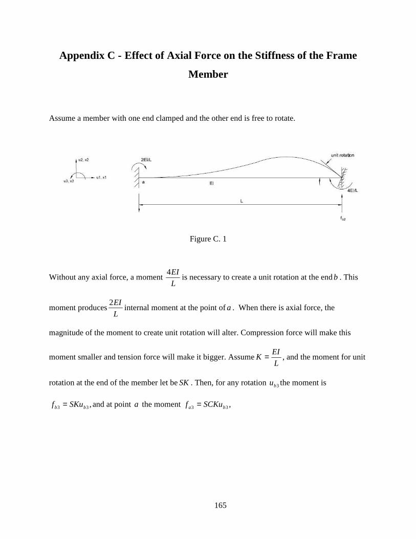
165
Appendix C - Effect of Axial Force on the Stiffness of the Frame
Member
Assume a member with one end clamped and the other end is free to rotate.
Figure C. 1
Without any axial force, a moment L
EI4is necessary to create a unit rotation at the endb . This
moment producesL
EI2internal moment at the point ofa . When there is axial force, the
magnitude of the moment to create unit rotation will alter. Compression force will make this
moment smaller and tension force will make it bigger. AssumeL
EIK = , and the moment for unit
rotation at the end of the member let beSK. Then, for any rotation 3bu the moment is
,33 bb SKuf = and at point a the moment ,33 ba SCKuf =

166
Figure C. 2
It is evident that Sand C reduce to 4and 5.0 correspondingly when 01 =af
Let 2
2
L
EIPE
π= , EP
P=ρ , L
EIK = , and ρπα
2=
=EP Euler load, and 11 ba ffP −==
Then, EI
fL
a12 =α (C.1)
Applying small deflection theory:
1232121
22
xffufdx
udEI aaa −=+ (C.2)
33 ba SCKuf = (C.3)
( ) ( )3
3332
1b
bbaa u
L
KCS
L
KuSCS
L
fff
+=+
=+
= (C.4)

167
By substituting equations (C.3) and (C.4) into (C.2) the following equation is obtained:
( )( ) 1
332
12
1
22 1
xLEI
KuCSu
EI
SCKu
EI
f
dx
ud bb
a +−=+ (C.5)
( )( ) 1
3322
2
21
22 14
xLEI
KuCSu
EI
SCKu
Ldx
ud bb
+−=+ α
(C.6)
Solution of (C.6) is:
( ) 11
3112 1
2sin
2cos xCCL
Lf
SKux
LBx
LAu
a
b +−++= αα (A.7)
Boundary conditions:
At 0,0 21 == ux ,0 31
Auf
SCKb
a
+= 31
ba
uf
SCKA
−=
,01
2 =dx
du
( )B
Lu
Lf
KCSb
a
α210 3
1
++−=
( )3
12
1b
a
uf
KCSB
α+=
( )[ ] ( )1
1
31
1
31
1
32
2sin
2
12cos1 x
Lf
KuCSx
Lf
SCKuxCCL
Lf
SKuu
a
b
a
b
a
b αα
α ++−+−= (C.8)
Rearrangement,
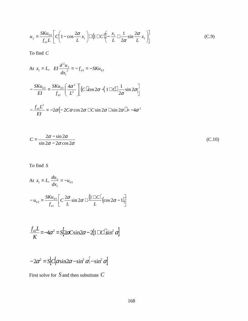
168
( )
+−++
−= 11
11
32
2sin
2
11
2cos1 x
LL
xCx
LC
Lf
SKuu
a
b αα
α (C.9)
To find C
At ,1 Lx = 3321
22
ba SKufdx
udEI −=−=
( ) ( )
+−
=− α
ααα
2sin2
112cos
42
2
1
33 CCLf
SKu
EI
SKu
a
bb
( ) 22
1 42sin2sin2cos22 αααααα −=++−−=− CCEI
Lfa
ααααα
2cos22sin
2sin2
−−=C (C.10)
To find S
At ,1 Lx = 31
2bu
dx
du−=
( ) ( )
−++=− 12cos1
2sin2
1
33 ααα
L
C
LC
f
SKuu
a
bb
( )[ ]αααα 221 sin122sin24 CCSK
Lfa +−=−=
( )[ ]ααααα 222 sinsin2sin2 −−=− CS
First solve for Sand then substitute C

169
( ) ααααα
22
2
sinsin2sin
2
−−−=
CS
( )( )( ) ( )ααααααααα
αααα2cos22sinsin2sin2sin2sin
2cos22sin222
2
−−−−−−=
( )ααααααααααααα
αααα2cossin22sinsin2sinsin2sinsin22sin2
2cos22sin2222222
2
+−+−−−−=
( )( ) ( )[ ]12cossin22sin22sin
2cos22sin22
2
−+−−−=
αααααααααα
( ) ( )ααααα
ααα
ααααααα
tansin2sincos22
2cot212
2sinsin42sin2
2cot21224 −−
−−=−−
−−=
( )( )ααααα
αααtansincossin
2cot21
+−−−=
Finally,
( )αα
ααα−
−=tan
2cot21S (C.11)
Now, the slope deflection equations (for no translation) can be written as:
jzijiz uSf = (C.12)
Where,
SSC
SCSKSij = and ba
j
i&=
(C.13)

170
Figure C. 3
For jointed member with rotation and translation can be written:
( )2213122121
22
abaaaa uuffxfufdx
udEI −+−=+ (C.14)
The solution is:
21
31
1
2112
2sin
2cos a
a
a
a
a uf
fx
f
fx
LBx
LAu +−++= αα
Boundary conditions:
,01 =x ,21
322 a
a
aa u
f
fAuu +−==
1
3
a
a
f
fA =

171
,2
1
23
1
2
a
aa f
fB
Lu
dx
du+== α
α21
23
L
f
fuB
a
aa
−=
The shear force,
( )L
uuf
L
fff ababa
a22133
2
−+
+=
21
31
22
1
331
22
1
3331
1
32
2sin
2
2cos a
a
aab
a
baab
a
baa
a
a uf
fx
L
uu
Lf
ffx
LL
uu
Lf
ffu
Lx
Lf
fu +−
−+
++
−−
+−+= α
αα
Let αα 2cos,2sin == tr
At ,1 Lx = 22 buu = and 31
2bu
dx
du=
( ) 21
322
1
3322
1
333
1
32 2 a
a
aab
a
baab
a
baa
a
ab u
f
fuu
f
ff
L
uu
Lf
ffu
Lrt
f
fu +−−+
++
−−
+−+=
α
( )[ ]2231
3
1
3
221
20 aba
a
b
a
a uuLurr
f
frt
f
f−−+
−+
−=ααα
(C.15)
( ) ( )L
uu
Lf
f
Lf
f
L
uu
Lf
ffut
f
f
L
ru ab
a
b
a
aab
a
baa
a
ab
22
1
3
1
322
1
333
1
33
2 −+++
−−
+−+×−= α
( ) ( ) ( ) ( ) 322
1
3
1
33 1121 a
ab
a
b
a
ab tut
L
uut
Lf
ftr
Lf
fu +−
−+−+−−= α
( ) ( ) ( )( ) 313122133 11210 baaaababa LufLtuftuuftftrf −+−−+−+−−= α (C.16)
To solve equations (C.15) and (C.16), multiply by ( )t−1 and ( )r−− α2 respectively.

172
( )( ) ( )( ) ( )( )( ) ( ) 3122133 1112120 aaababa utLrfrtuuftrftrtf −+−−−−−+−−= αα
( )( ) ( )( ) ( )( )( ) ( )( ) 31
3122133
2
221122210
ba
aaababa
urLf
urLtfrtuuftrfrtrf
−+−−−−−−−−−−−−−=
αααααα
( )( ) ( )( )[ ] ( ) ( ) ( ) ( )( ) ( )( )[ ] 0211
22122112 22131313
=−−+−×−+−+−−−+−−−−−−
rttr
uufrLufrttrLufrtrtrtf ababaaaa
αααααα
This can be written as:
( ) 0221431331231 =−+++ ababaaaa uufALufALufAfA (C.17)
( )( ) ( )( )( ) ( )rttrrtt
rtrrtrrtrttrtrtrtA
αααααααααααααααα
+−=++−+−=
−−+++−+−−=−−−−−−=
1424222
22422222112222
2221
( ) ( ) ( )trrttrtrrttrA ααα 22212 −=+−−=−−−=
rA −= α23
( ) ( )( ) ( )12222114 −=+−−+−=−−+−= trrttrrtrttrA αααα
Substituting these coefficients into equation (C.17) and solving for 3af
( )( )
( )( )
( )( ) ( )22
13
13
13 12
1
14
2
14
2ab
ab
aa
aa uu
rt
ftu
rt
Lfru
rt
Ltrff −
−−−
+−−
−+
−−−
=ααα
ααα
α (C.18)
To get ,3bf substitute equation (C.18) into equation (C.15),
( )( )( )
( )( )( )
( )( )( ) ( ) ( )
( )22131
3221
31 2
12
12
14
212
14
220
abaaa
baba
aa
uurfLruf
rfuurt
trt
rt
Lfrtu
rt
Lftrrt
−−
−+−−−
−−+−−−−
+−−
−−= α
αα
αααα
αααα
( ) ( )( )( )
( )( )( ) ( )
( )( )( )
−−−
−−
×−+
−−−−+
+−−−−=−
rrt
trt
uufrt
rrtLufr
rt
trrtLuffr ababaaab
αα
αααα
ααααα
12
12
14
22
14
222 22131313
( ) ( ) ( ) ( )( )322123113132 BuufBLufBLuffr ababaaab −++=− α (C.19)

173
( )rt
rrtrrttrB
ααααααα
−−−++−−=
14
44242 22222
1
( )( )
( )( )rt
r
rt
rrrtB
ααα
αααα
−−−−=
−−+−+−=
14
2
14
44 22222
1
( )( )( )rt
rrtB
αααα
−−−−=
14
222
( )( )( ) ( )
( )( )( )rt
rt
rt
rrtrrrtttr
rt
trtB
αα
αααα
αα
−−−−=
−−++−+−−=−
−−−−=
12
21
12
22222
12
12 22
3
( )( )
( )( )
( )( ) ( )22
13
13
13 12
1
14
2
14
2ab
ab
aa
ab uu
rt
ftu
rt
Lftru
rt
Lfrf −
−−−
+−−
−+
−−−
=ααα
ααα
α (C.20)
It is observable that (C.18) and (C.20) are slope deflection equations. The next step is to express
the coefficients of the displacements in terms of the coefficients of slope deflection equations
without any axial load but modified by .iβ
Let,
( )223232313
624abbaa uu
L
EIu
L
EIu
L
EIf −
−
+
= βββ (C.21)
( )223231323
642abbab uu
L
EIu
L
EIu
L
EIf −
−
+
= βββ (C.22)
Therefore,

174
( )( )rt
Lftr
L
EI a
αααβ
−−−
=
14
24 11
( )( )rt
Lfr
L
EI a
αααβ
−−−
=
14
22 12
( )( )rt
ft
L
EI a
αβ
−−−
=
12
16 132
Solving for ,iβ the following is obtained:
( )( ) ( )rtEI
Lftr a
αααβ
−−−
=144
2 21
1
(C.23)
( )( ) ( )
( )( )
( ) ( )( )
( )( )
××−−×
−−=
−−−=
−−−
=22sin
2sin
2cot21
2cot21
2sinsin2
2sin2
2sin2cos18
42sin2
18
22
221
2
ααα
αααα
ααααα
αααααα
αααβ
rtEI
Lfr a
( ) ( )( ) 22cos22sin
2cot21
2sin
sin2
2sin2
2 2
SC=−
−
−
−
=ααα
αα
ααα
ααα (C.24)
( )( )
( )( ) ( )αα
α
ααααα
αβ
cot13
1
2sin2cos1
12cos
3112
12
221
3 −
=−−
−−
=
−−−−
=rtEI
Lft a (C.25)
Define ααβ cot5 =
( )( ) 4tan
2cot21
42sinsin2
2cos22sin
42sin2cos116
42cos22sin2
2
1
S=−
−
=
−−
=−−
−=αα
αααααααααα
ααααααααβ

175
[ ]355
2
5
5
51 3
4
1
1
cot2
1cot21
41
2cot21
4tan
2cot21
44ββ
βα
ααβ
βααβ
αααααβ +=
−
−−×=
−−×=
−−×== S
(C.27)
Similarly,
[ ]532 32
1 βββ −= (C.28)
Therefore, 3β can be expressed in terms of Sand C
3533521 63324 βββββββ =−++=+
[ ] ( )6
124
6
1213
CS +=+= βββ (C.29)
The equilibrium condition for the member is:
( )221332 ababaa uufffLf −++= (C.30)
or
( ) 3122232212221
332
422412baab
aa u
L
EI
L
EIu
L
EI
L
EIuu
L
f
L
EIf
++
++−
+−= βββββ
This can be written as:
( )L
f
L
EI
L
EIu
L
EIu
L
EIuu
L
EIf a
baaba1
334337237222432
12126612 +−=−
+
+−
−= βββββ
−−
=−=−= 1
cot1
1
3312
22
32
221
34 ααααβ
ππββ
EI
Lf a
35
2
4 cot1
cot
3ββ
αααααβ ×=
−
= (C.31)
And 3217 6246 ββββ =+=
176
37 ββ = (C.32)
These derivations are based on the assumption that the axial force 1af on the member is
compressive. If the axial force is tensile, then the trigonometric functions in the stability
functions Sand C and iβ all become hyperbolic functions.