el niño-southern oscillation during the past 50 years
TRANSCRIPT
University of Wollongong University of Wollongong
Research Online Research Online
Faculty of Science, Medicine & Health - Honours Theses University of Wollongong Thesis Collections
2012
El Niño-Southern Oscillation during the past 50 years: El Niño-Southern Oscillation during the past 50 years:
Jessica Jean Gaudry University of Wollongong
Follow this and additional works at: https://ro.uow.edu.au/thsci
University of Wollongong University of Wollongong
Copyright Warning Copyright Warning
You may print or download ONE copy of this document for the purpose of your own research or study. The University
does not authorise you to copy, communicate or otherwise make available electronically to any other person any
copyright material contained on this site.
You are reminded of the following: This work is copyright. Apart from any use permitted under the Copyright Act
1968, no part of this work may be reproduced by any process, nor may any other exclusive right be exercised,
without the permission of the author. Copyright owners are entitled to take legal action against persons who infringe
their copyright. A reproduction of material that is protected by copyright may be a copyright infringement. A court
may impose penalties and award damages in relation to offences and infringements relating to copyright material.
Higher penalties may apply, and higher damages may be awarded, for offences and infringements involving the
conversion of material into digital or electronic form.
Unless otherwise indicated, the views expressed in this thesis are those of the author and do not necessarily Unless otherwise indicated, the views expressed in this thesis are those of the author and do not necessarily
represent the views of the University of Wollongong. represent the views of the University of Wollongong.
Recommended Citation Recommended Citation Gaudry, Jessica Jean, El Niño-Southern Oscillation during the past 50 years:, Bachelor of Environmental Science (Honours), School of Earth & Environmental Science, University of Wollongong, 2012. https://ro.uow.edu.au/thsci/78
Research Online is the open access institutional repository for the University of Wollongong. For further information contact the UOW Library: [email protected]

El Niño-Southern Oscillation during the past 50 years: El Niño-Southern Oscillation during the past 50 years:
Abstract Abstract Atmospheric and oceanographic fluctuations across the tropical Pacific Ocean are partly a function of the phenomena known as the El Niño Southern Oscillation (ENSO), which is recognised as the strongest signal of interannual climate variation in the world. Pioneering studies, which utilise recent living corals
from Tarawa (1oN, 172oE) and Maiana (1oN, 173oE), in the western equatorial Pacific Ocean, indicate that
coral oxygen isotope (δ18O) records from this region can be used to reflect variations in ENSO-related
climate patterns (Cole et al. 1993; Urban et al. 2000). The δ18O signal, however, is a combination of both
changes in sea surface temperature (SST) and in the δ18O of seawater (δ18Osw), yet both these factors may change with ENSO variations. This study investigates the coral-derived climate signals of the past 50
years (~1960 to 2010) from Butaritari Atoll (~172o30’E, 3o30’N) located in the western central equatorial
Pacific using paired Sr/Ca and δ18O proxies to separate the SST and δ18Osw signals. The Sr/Ca-derived
SST results show a warming trend of 0.77 ± 0.17 oC and that decadal variability dominates over
interannual. The Butaritari δ18Osw results provide additional climatic information about the balance of evaporation and precipitation, although no significant freshening trend is evident. Taken together, the
Butaritari Sr/Ca-derived SST and δ18Osw results suggest the warming and/or freshening trends observed
in coral δ18O reflect predominantly changes in SST for the past 50 years. The Butaritari SST trend is also consistent with Sr/Ca estimates from central equatorial Pacific islands and suggests warming at broader scale.
Degree Type Degree Type Thesis
Degree Name Degree Name Bachelor of Environmental Science (Honours)
Department Department School of Earth & Environmental Science
Advisor(s) Advisor(s) Helen McGregor
Keywords Keywords equatorial, oxygen isotope, stronium calcium
This thesis is available at Research Online: https://ro.uow.edu.au/thsci/78

El Niño-Southern Oscillation during the past 50 years:
Reconstructions from a western Pacific coral
Jessica Jean Gaudry
A research report submitted in partial fulfilment of the requirements for
the award of the degree of
HONOURS BACHELOR OF ENVIRONMENTAL SCIENCE
ENVIRONMENTAL SCIENCE PROGRAM
FACULTY OF SCIENCE
UNIVERSITY OF WOLLONGONG
October 2012


i
ACKNOWLEDGEMENTS
I would like to extend a huge thankyou to Dr Helen McGregor for her constant
enthusiasm, encouragement and many words of wisdom. Her support over the past year
has been flawless.
I also wish to thank Dr Jessica Carilli for collecting the Butaritari coral used in this
thesis and for her support and input throughout the project. Thank you to Henri Wong
and Matthew Dore for running the ICP-AES analysis at the Australian Nuclear Science
and Technology Organisation (ANSTO) and their assistance in understanding the Excel
output. Thank you to Joan Cowley and Heather Scott-Gagan at the Australian National
University (ANU) for running my !18O samples. Thanks to José Abrantes, Geoff Hurt,
David Wheeler and Lily Yu for their technical support throughout the sample
preparation stage. Thank you to Harry Schofield and Laurent Devriendt for their
assistance in the coral laboratory. Thanks to Rittick Borah for his help with statistical
software. Finally I would like to thank my family and friends for their endless support
and for keeping me (partly) sane.

ii
ABSTRACT
Atmospheric and oceanographic fluctuations across the tropical Pacific Ocean are partly
a function of the phenomena known as the El Niño Southern Oscillation (ENSO), which
is recognised as the strongest signal of interannual climate variation in the world.
Pioneering studies, which utilise recent living corals from Tarawa (1oN, 172oE) and
Maiana (1oN, 173oE), in the western equatorial Pacific Ocean, indicate that coral oxygen
isotope (!18O) records from this region can be used to reflect variations in ENSO-
related climate patterns (Cole et al. 1993; Urban et al. 2000). The !18O signal, however,
is a combination of both changes in sea surface temperature (SST) and in the !18O of
seawater (!18Osw), yet both these factors may change with ENSO variations. This study
investigates the coral-derived climate signals of the past 50 years (~1960 to 2010) from
Butaritari Atoll (~172o30’E, 3o30’N) located in the western central equatorial Pacific
using paired Sr/Ca and !18O proxies to separate the SST and !18Osw signals. The Sr/Ca-
derived SST results show a warming trend of 0.77 ± 0.17 oC and that decadal variability
dominates over interannual. The Butaritari !18Osw results provide additional climatic
information about the balance of evaporation and precipitation, although no significant
freshening trend is evident. Taken together, the Butaritari Sr/Ca-derived SST and !18Osw
results suggest the warming and/or freshening trends observed in coral !18O reflect
predominantly changes in SST for the past 50 years. The Butaritari SST trend is also
consistent with Sr/Ca estimates from central equatorial Pacific islands and suggests
warming at broader scale.

iii
TABLE OF CONTENTS
ACKNOWLEDGEMENTS ........................................................................................... i!
ABSTRACT ................................................................................................................ ii!
TABLE OF CONTENTS ........................................................................................... iii!
LIST OF FIGURES ...................................................................................................... v!
LIST OF TABLES .................................................................................................... xiii!
1.! INTRODUCTION ............................................................................................... 14!
2.! LITERATURE REVIEW .................................................................................... 16!
2.1! Tropical Pacific climate ................................................................................. 16!
2.1.1! El Niño Southern Oscillation .................................................................. 16!
2.1.2! Western equatorial Pacific ..................................................................... 17!
2.2! Climate reconstruction using corals .............................................................. 21!
2.3! Regional setting: Butaritari Atoll, Kiribati .................................................... 24!
2.3.1! Local climatology ................................................................................... 26!
3.! MATERIALS AND METHODS ........................................................................ 28!
3.1 Coral collection ................................................................................................. 28!
3.2 X-Radiography ................................................................................................. 29!
3.3 Coral dating and preservation ........................................................................... 32!
3.4 Sample preparation ........................................................................................... 32!
3.5 Sr/Ca analysis ................................................................................................... 33!
3.6 Isotope analysis ................................................................................................. 35!
3.7 Assigning chronology ....................................................................................... 36!
4. RESULTS ............................................................................................................... 38!
4.1 Butaritari geochemistry .................................................................................... 38!
5. DISCUSSION ......................................................................................................... 41!
5.1 Calibrating Sr/Ca to SST .................................................................................. 41!
5.1.1 Potential calibration uncertainties ............................................................ 44!
5.1.2 Sr/Ca-derived SST ..................................................................................... 47!
5.2 Deciphering SSS from !18O using coral-derived SST ...................................... 48!
5.3 Coral geochemistry compared to local climatology ......................................... 51!
5.3.1 Wavelet analysis ........................................................................................ 55!

iv
5.4 Butaritari compared to Tarawa and Maiana ..................................................... 61!
5.5 Butaritari compared to other Pacific records .................................................... 69!
CONCLUSIONS AND RECOMMENDATIONS ..................................................... 75!
REFERENCES ........................................................................................................... 78!
APPENDIX: (Data CD) .............................................................................................. 87!

v
LIST OF FIGURES
Figure 1 – NINO regions of the Pacific Ocean (Australian Bureau of Meteorology
2012b). NINO 4 region covers the area 5oN-5oS, 160oE-150oW and contains
Butaritari Atoll (yellow circle; ~172o30’E, 3o30’N), the area of interest in this
study. ....................................................................................................................... 17!
Figure 2 – Colour enhanced image of 10-year mean (1982 to 1991) SST from satellite
data. The warmest temperatures evident in the Western Pacific Warm Pool (dark
orange and red colours correspond to SST higher than 28oC; from Yan et al. 1992).
................................................................................................................................ 18!
Figure 3 – a) The IPWP in February (blue) and September (red) as given by the 28!C
isotherm based on the long-term (1900–2009) mean SST from the HadISST
dataset. (b) Seasonal variation of the WPWP size (blue) and maximum SST (red)
respectively. Units for the size and SST are 107 km2 and !C, respectively (from
Bolan and Lixin 2012). ........................................................................................... 19!
Figure 4 – Migration of the eastern edge of the Western Pacific Warm Pool. Left panel
is the longitude-time distribution of 4oN-4oS averaged SST, and the right panel is
SSS for the same area. The thick white line is the Southern Oscillation Index
(SOI). Sustained positive and negative SOI correspond to La Niña and El Niño
phases, respectively. Contours are 1oC for SST and 0.25 psu for SSS. Dark shading
in the left and right panels indicates higher SST and higher SSS, respectively.
Orange lines indicate the longitudinal positions of Butaritari Atoll (~172o30’E,
3o30’N; this study), Tarawa (1oN, 172oE) and Maiana (1oN, 173oE). (Modified
from Picaut et al. 2001). ......................................................................................... 20!
Figure 5 – Republic of Kiribati (Australian Bureau of Meteorology and CSIRO 2011).
Butaritari Atoll is highlighted by the red rectangle and is located at ~172030’E,
3030’N, just north of the capital of Kiribati, Tarawa. ............................................. 25!
Figure 6 – A typical fore reef environment throughout the Gilbert Islands (Carilli pers.
comm.). Dominant genera include Porites, Pocillopora, Acropora, Heliopora and
crustose coralline algae (CCA). .............................................................................. 25!
Figure 7 - Mean monthly SST for the time period between 1959 to 2010 derived from
ERSSTv3b (Smith et al. 2008. Black contours = 0.5oC. The location of Butaritari

vi
(this study; 3o30’N, 172o30’E) is indicated by a yellow circle. The locations of
Tarawa (1oN, 172oE) and Maiana (1oN, 173oE) are indicated by a red square and
green star respectively. ........................................................................................... 27!
Figure 8 – Mean precipitation data for the time period between January 1979 to
November 2011 derived from CMAP Precipitation data from NOAA NCEP CPC
Merged Analysis monthly latest version 1 precipitation estimate (Xie and Arkin
1996; Xie and Arkin 1997). The location of Butaritari (this study; 3o30’N,
172o30’E) is indicated by a yellow circle. The locations of Tarawa (1oN, 172oE)
and Maiana (1oN, 173oE) are indicated by a red square and purple star respectively.
................................................................................................................................ 27!
Figure 9 – Map of Butaritari Atoll, Kiribati (~172o30’E, 3o30’N; N. Biribo pers.
comm.). The yellow circle indicates the location of the modern coral used in this
study. ....................................................................................................................... 28!
Figure 10 – The underwater drilling of the Porites sp. modern coral (BUT3-2) from the
fore reef on the southern side of Butartari Atoll, Kiribati (~172o30’E, 3o30’N). The
top surface of the coral was approximately 4 m underwater. A coral core
approximately 83 cm in length and 4.5 cm in diameter was collected. .................. 29!
Figure 11 – X-ray positive images of the Butaritari modern coral (BUT3-2). The coral
pieces are ordered sequentially such that the top surface of piece 1 is the youngest
surface of the coral core, and the bottom of piece 7 is the oldest surface of the core.
Red lines correspond to the maximum growth axis, and thus indicate the position
of sampling transects used for both Sr/Ca and !18O geochemical analysis. ........... 31!
Figure 12 – Preliminary bulk Sr/Ca samples test results for the Butaritari modern coral.
Samples with weights of ~0.5 mg are represented by a triangle symbol and ~0.75
mg samples by a square symbol. Samples were measured from BUT3-2 piece 3
(blue symbols), BUT3-2 piece 5 (red symbols), and BUT3-2 piece 6 (green
symbols). ................................................................................................................. 35!
Figure 13 - SST (ERSSTv3b; Smith et al. 2008) for the 2o x 2o grid square at 2oN,
172oE containing Butaritari for the period between 1959 and 2010. Monthly SST
(red line) is compared to bi-monthly SST, derived from interpolation of monthly
data (blue line). The bi-monthly SST trace overlies the monthly SST trace. ......... 37!

vii
Figure 14 – Butaritari coral geochemistry (BUT3-2); Sr/Ca (red line), !18O (green line)
and !13C (black line). Note: inverted y-axes. All values have been derived from
along the same sampling transect. .......................................................................... 38!
Figure 15 – Time series of Butaritari coral geochemistry (BUT3-2); Sr/Ca (red line)
and !18O (green line), using ERSSTv3b SST data for the 2o x 2o grid square at 2oN,
172oE containing Butaritari (blue line; Smith et al. 2008). Note: inverted y-axes for
Sr/Ca and !18O. All data including SST have been interpolated to a bi-monthly
resolution corresponding to 6 data points per year. ................................................ 39!
Figure 16 – Sr/Ca and "18O residuals with the annual cycle removed for the period
between 1959 and 2010. ......................................................................................... 40!
Figure 17 – Bi-monthly Sr/Ca values of the Butaritari modern coral (BUT3-2)
compared to bi-monthly SST. SST is from ERSSTv3b (Smith et al. 2008) for the
2o x 2o grid square at 2oN, 172oE, which includes Butaritari Island. Solid filled
circles and coloured squares indicate the maxima and minima points used in the
Sr/Ca-SST calibration (n = 90). These solid filled points are on average at an
annual resolution corresponding to the summer maximum and winter minimum
values for each year. The pair of green squares denotes the maxima point in the
Sr/Ca record and the corresponding point in SST. The pair of orange squares
denotes the minima point in the Sr/Ca record and the corresponding point in SST.
The pair of pink squares denotes the minima SST point and the corresponding
point in Sr/Ca. The pair of yellow squares denotes the maxima point in the SST
record and the corresponding point in Sr/Ca. ......................................................... 42!
Figure 18 – Butaritari modern coral (BUT3-2) Sr/Ca-SST calibration points and
equation. Red crosses indicate the Sr/Ca values and corresponding SST from
Figure 17. Blue line is a linear regression through the Sr/Ca-SST points. Green
circle denotes the maxima Sr/Ca value and orange circle denotes the Sr/Ca minima
value (Also shown in Figure 17). .......................................................................... 43!
Figure 19 – Modern Butaritari Sr/Ca-SST reconstructions. Blue line is SST for
Butarirari (ERSSTv3b; Smith et al. 2008). Red line is the coral-derived estimates
of SST, calculated from the Butaritari Sr/Ca-SST relationship: Sr/Ca = 10.904 –
0.0688 * SST (r2 = 0.5818). A line of best fit has been fitted to both datasets. Black

viii
dotted line is monthly IGOSS SST for the 1o x1o grid square at 171.5oE, 2.5oN,
containing Butaritari (Reynolds et al. 2002). ......................................................... 44!
Figure 20 – Monthly observation counts for data points used in the International
Comprehensive Ocean Atmosphere Data Set (ICOADS), from which ERSSTv3b is
derived (Research Data Archive 2012). ................................................................. 45!
Figure 21 – Modern Butaritari coral geochemistry compared to local climatology and
ENSO indices. a) Butaritari "18O (green). b) Butaritari Sr/Ca-derived SST (red). c)
Butaritari #"18Osw (blue). d) SST (red) from ERSSTv3b (Smith et al. 2008) for the
2o x 2o grid square at 2oN, 172oE. The SST dataset has been interpolated to bi-
monthly resolution to correspond with the resolution of the coral geochemistry
data. e) Normalised mean daily Butaritari precipitation for each month from
NOAA NCDC GCPS MONTHLY STATION mean precipitation (Baker et al.
1994) for 1959 to 1982 (light blue) from Butaritari, station ID 9160100, at 3.03N,
172.78E; and monthly CMAP Estimated Precipitation (Xie and Arkin 1996; Xie
and Arkin 1997) for 1979 to 2010 (dark blue) for the 2.5o x 2.5o grid square at
1.25N, 171.25W. f) Monthly SSS (at 5.01 meters depth) from CARTON-GIESE
SODA latest version (v2p1p6) for the 0.5o x 0.5o grid square at 172.25E 3.25N
containing Butaritari Island (Carton and Giese 2008). g) Monthly NINO 4 data
(yellow) for the NINO 4 region (5oN-5oS, 160oE-150oW) sourced from
http://www.cpc.ncep.noaa.gov. h) Monthly SOI data (pink) sourced from the
Australian Bureau of Meteorology
(http://www.bom.gov.au/climate/current/soi2.shtml). El Niño threshold (SOI < -8;
Australian Bureau of Meteorology 2012a) is marked by a dotted line on the SOI
trace. La Niña threshold (SOI > 8) is marked by a dashed line on the SOI trace. El
Niño events (SOI < -8 for sustained periods) are shaded dark grey. La Niña events
(SOI > 8 for sustained periods) are shaded light grey. Note: inverted y-axes for a),
c), f) and h). ............................................................................................................ 53!
Figure 22 – Modified version of Figure 4. Migration of the eastern edge of the Western
Pacific Warm Pool. Left panel is the longitude-time distribution of 4oN-4oS
averaged SST, and the right panel is SSS for the same area. The thick white line is
the Southern Oscillation Index (SOI). Sustained positive and negative SOI
correspond to La Niña and El Niño phases, respectively. Contours are 1oC for SST
ix
and 0.25 psu for SSS. Dark shading in the left and right panels indicates higher
SST and higher SSS, respectively. Orange lines indicate the longitudinal positions
of Butaritari Atoll (~172o30’E, 3o30’N; this study), Tarawa (1oN, 172oE) and
Maiana (1oN, 173oE). (Modified from Picaut et al. 2001). Blue shaded areas
correspond to years of slight misalignment between Butaritari coral and ENSO
indices evident in Figure 21). ................................................................................ 55!
Figure 23 – Part 1 and 2 is wavelet analysis for Butaritari coral "18O and Sr/Ca-derived
SST, respectively. (a) Coral record. (b) The wavelet power spectrum (Torrence and
Compo 1998), red indicates areas of highest power. The contour levels are chosen
so that 75%, 50%, 25%, and 5% of the wavelet power is above each level,
respectively. The cross-hatched region is the cone of influence, where zero padding
has reduced the variance. (c) The global wavelet power spectrum, which is the
average variance of each period for the whole time series. Grey shading
corresponds to annual variance; purple shading corresponds to interannual (2-8
years) variance; and orange shading corresponds to ~decadal variance. ............... 57!
Figure 24 – (a) NINO4 anomaly. (b) The wavelet power spectrum (Torrence and
Compo 1998), red indicates areas of highest power. The contour levels are chosen
so that 75%, 50%, 25%, and 5% of the wavelet power is above each level,
respectively. The cross-hatched region is the cone of influence, where zero padding
has reduced the variance. (c) The global wavelet power spectrum, which is the
average variance of each period for the whole time series. Grey shading
corresponds to annual variance; purple shading corresponds to interannual (2-8
years) variance; and orange shading corresponds to ~decadal variance. ............... 59!
Figure 25 – (a) SOI. (b) The wavelet power spectrum (Torrence and Compo 1998), red
indicates areas of highest power. The contour levels are chosen so that 75%, 50%,
25%, and 5% of the wavelet power is above each level, respectively. The cross-
hatched region is the cone of influence, where zero padding has reduced the
variance. (c) The global wavelet power spectrum, which is the average variance of
each period for the whole time series. Grey shading corresponds to annual
variance; purple shading corresponds to interannual (2-8 years) variance; and
orange shading corresponds to ~decadal variance. ................................................ 59!

x
Figure 26 – (a) SST (ERSSTv3b; Smith et al. 2008). (b) The wavelet power spectrum
(Torrence and Compo 1998), red indicates areas of highest power. The contour
levels are chosen so that 75%, 50%, 25%, and 5% of the wavelet power is above
each level, respectively. The cross-hatched region is the cone of influence, where
zero padding has reduced the variance. (c) The global wavelet power spectrum,
which is the average variance of each period for the whole time series. Grey
shading corresponds to annual variance; purple shading corresponds to interannual
(2-8 years) variance; and orange shading corresponds to ~decadal variance. ........ 60!
Figure 27 – Coral "18O records from three western equatorial Pacific islands. A) 1840
to 2000. Green dotted line corresponds to bi-monthly Butaritari (3o30’N, 172o30’E
) "18O data from this study. Blue dotted line corresponds to monthly Tarawa (1oN,
172oE) !18O data from Cole et al. (1993). Red dotted line corresponds to bi-
monthly Maiana (1oN, 173oE) !18O data from Urban et al. (2000). Solid lines
correspond to moving averages (12 point for Butaritari and Maiana, and 24 point
for Tarawa), which remove < 2 year variability from the data. Black bracket
indicates the area of overlap with the Butaritari record. B) Same as for A) except
for 1959 to 2000, the area of overlap with the Butaritari record. Monthly SOI data
(pink) sourced from the Australian Bureau of Meteorology
(http://www.bom.gov.au/climate/current/soi2.shtml). El Niño threshold (SOI < -8)
is marked by a dotted line on the SOI trace. La Niña threshold (SOI > 8) is marked
by a dashed line on the SOI trace. El Niño events (SOI < -8 for sustained periods)
are shaded dark grey. La Niña events (SOI > 8 for sustained periods) are shaded
light grey. ................................................................................................................ 62!
Figure 28 – (a) Tarawa "18O for the period of overlap with the Butaritari record. (b) The
wavelet power spectrum (Torrence and Compo 1998), red indicates areas of
highest power. The contour levels are chosen so that 75%, 50%, 25%, and 5% of
the wavelet power is above each level, respectively. The cross-hatched region is
the cone of influence, where zero padding has reduced the variance. (c) The global
wavelet power spectrum, which is the average variance of each period for the
whole time series. Grey shading corresponds to annual variance; purple shading
corresponds to interannual (2-8 years) variance; and orange shading corresponds to
~decadal variance. .................................................................................................. 64!

xi
Figure 29 – (a) Maiana "18O for the period of overlap with the Butaritari record. (b) The
wavelet power spectrum (Torrence and Compo 1998), red indicates areas of
highest power. The contour levels are chosen so that 75%, 50%, 25%, and 5% of
the wavelet power is above each level, respectively. The cross-hatched region is
the cone of influence, where zero padding has reduced the variance. (c) The global
wavelet power spectrum, which is the average variance of each period for the
whole time series. Grey shading corresponds to annual variance; purple shading
corresponds to interannual (2-8 years) variance; and orange shading corresponds to
~decadal variance. .................................................................................................. 65!
Figure 30 – Zoomed in section of Figure 8. Mean precipitation data for the time period
between January 1979 to November 2011 derived from CMAP Precipitation data
from NOAA NCEP CPC Merged Analysis monthly latest version 1 precipitation
estimate (Xie and Arkin 1996; Xie and Arkin 1997). The location of Butaritari
(this study; 3o30’N, 172o30’E) is indicated by a yellow circle. The locations of
Tarawa (1oN, 172oE) and Maiana (1oN, 173oE) are indicated by a red square and
purple star respectively. Central Pacific islands: Palmyra (blue rectangle; 6oN,
162oW), Fanning (black rectangle; 4oN, 159oW) and Christmas (orange rectangle;
2oN, 157oW). ........................................................................................................... 66!
Figure 31 – Zoomed in section of (Figure 7). Mean monthly SST for the time period
between 1959 to 2010 derived from ERSSTv3b (Smith et al. 2008). Black contours
= 0.5oC. The location of Butaritari (this study; 3o30’N, 172o30’E) is indicated by a
yellow circle. The locations of Tarawa (1oN, 172oE) and Maiana (1oN, 173oE) are
indicated by a black square and purple star respectively. Central Pacific islands:
Palmyra (blue rectangle; 6oN, 162oW), Fanning (black rectangle; 4oN, 159oW) and
Christmas (orange rectangle; 2oN, 157oW). ........................................................... 67!
Figure 32 – "18O records and trend lines for Butaritari (green), Tarawa (blue) and
Maiana (red). The Tarawa and Maiana data are from longer datasets however they
have been truncated to the period of overlap with the Butaritari record (see Figure
27). The black bracket indicates the common interval between all three datasets. 67!
Figure 33 – Coral "18O records from three western (a) and three central (b) equatorial
Pacific islands. a) "18O records from Butaritari (green line; bi-monthly resolution;
3o30’N, 172o30’E; this study), Tarawa (blue line; monthly resolution; 1oN, 172oE;

xii
Cole et al. 1993) and Maiana (red line; bi-monthly resolution; 1oN, 173oE; Urban
et al. 2000) islands between 1959 and 1990. b) "18O records from Palmyra (pink
line; monthly resolution; 6oN, 162oW; Cobb et al. 2001), Fanning (black line;
monthly resolution; 4oN, 159oW; Nurhati et al. 2009) and Christmas (orange line;
monthly resolution; 2oN, 157oW; Nurhati et al. 2009) islands between 1972 and
1998; Christmas between 1959 and 1993 (Evans et al. 1998), and between 1978
and 2007 (McGregor et al. 2011). c) Monthly Southern Oscillation Index (SOI)
available from the Australian Bureau of Meteorology
(http://www.bom.gov.au/climate/current/soi2.shtml). El Niño threshold (SOI < -8)
is marked by a dotted line on the SOI trace. La Niña threshold (SOI > 8) is marked
by a dashed line on the SOI trace. The black bracket indicates the common interval
between datasets (1972-1998). ............................................................................... 71!
Figure 34 – Coral Sr/Ca-derived SST records from one western (a) and three central (b)
equatorial Pacific islands. a) Sr/Ca-derived SST record from Butaritari (green line;
bi-monthly resolution; 3o30’N, 172o30’E; this study) between 1959 and 1990. b)
Sr/Ca-derived SST records from Palmyra (pink line; monthly resolution; 6oN,
162oW; Cobb et al. 2001), Fanning (black line; monthly resolution; 4oN, 159oW;
Nurhati et al. 2009) and Christmas (orange line; monthly resolution; 2oN, 157oW;
Nurhati et al. 2009) islands between 1972 and 1998. c) Monthly Southern
Oscillation Index (SOI) as described in Figure 33. The black bracket indicates the
common interval between datasets (1972-1998). ................................................... 73!
Figure 35 – Relative variations in !18Osw records (SSS proxy) from one western (a) and
three central (b) equatorial Pacific islands. a) !18Osw record from Butaritari (green
line; bi-monthly resolution; 3o30’N, 172o30’E; this study) between 1959 and 1990.
b) !18Osw records from Palmyra (pink line; monthly resolution; 6oN, 162oW; Cobb
et al. 2001), Fanning (black line; monthly resolution; 4oN, 159oW; Nurhati et al.
2009) and Christmas (orange line; monthly resolution; 2oN, 157oW; Nurhati et al.
2009) islands between 1972 and 1998. c) Monthly Southern Oscillation Index
(SOI) as described in Figure 33. ............................................................................ 74!

xiii
LIST OF TABLES
Table 1 – ICP-OES instrument settings for Sr/Ca runs in this study. ........................ 34!
Table 2 – Preliminary Butaritari bulk Sr/Ca samples test results. ............................. 35!
Table 3 - "18O trends in Butaritari (this study), Tarawa (Cole et al. 1993) and Maiana
(Urban et al. 2000) for the common data interval (1959-1990) and overall (1959-
2010 for Butaritari and 1959-1994 for Maiana). ................................................ 69!
Table 4 - Butaritari (this study), Tarawa (Cole et al. 1993) and Maiana (Urban et al.
2000), Palmyra, Fanning and Christmas (Nurhati et al. 2009) "18O trends. ...... 70!
Table 5 - Butaritari (this study), Palmyra, Fanning and Christmas (Nurhati et al. 2009)
Sr/Ca-SST trends. ............................................................................................... 72!
Table 6 - Butaritari (this study), Palmyra, Fanning and Christmas (Nurhati et al. 2009)
!18Osw trends. ...................................................................................................... 73!

14
1. INTRODUCTION
El Niño Southern Oscillation (ENSO), has been recognised as the strongest signal of
interannual climate variation in the world (Wang et al. 1999). While ENSO primarily
occurs within the tropics, it has also been recognised to influence global climate
through atmospheric teleconnections (Philander 1990). ENSO forcing of both the
atmosphere and ocean is strongest in the west/central equatorial Pacific between
approximately 150oE and 150oW (Clarke 2008). The western equatorial Pacific is
recognised by warm and fresh water, primarily corresponding to the Indo-Pacific
Warm Pool (IPWP) (Yan et al. 1992). This large body of warm water plays in an
integral role in convection patterns across the Pacific. Changes in the IPWP can be
attributed to variability in solar radiance, ENSO events, atmospheric aerosols (from
volcanic activity) and global warming (Yan et al. 1992).
Despite the Pacific region having a major influence on global climate, short and
sparse instrumental datasets limit the investigation of climatic patterns across this
region. The skeletal material of modern and fossil coral can be used as a high
resolution geochemical record to reconstruct localised climatic information (Cohen
and McConnaughey 2003). Previous work based on !18O in corals from Tarawa (1oN,
172oE; Cole and Fairbanks 1990; Cole et al. 1993) and Maiana (1oN, 173oE; Urban et
al. 2000) Islands, located close to Butaritari Island (~172o30’E, 3o30’N) and at the
eastern edge of the Indo-Pacific Warm Pool (IPWP), show that this region is sensitive
to ENSO. Cole et al. (1993) used spectral analysis of a 96 year long coral record to
show shifts in the distribution of variance between annual and interannual periods
within the twentieth century. These observed changes suggest variation in the strength
of the ENSO signal over time. The Maiana coral record reflects a gradual transition of
ENSO variability in the early twentieth century and abrupt shift in 1976, both towards
warmer and wetter climatic conditions (Urban et al. 2000). Changes of ~2.9 to 4 year
periodicity of ENSO have also been noted to occur during this time. These studies
indicate that ENSO variability can change even with only small climatological
changes. One limitation of these studies is that they only use !18O to interpret these
climatic variations. The !18O signal reflects both changes in sea surface temperature

15
(SST) and in the !18O of seawater (!18Osw), which corresponds to the balance of
evaporation/precipitation (Swart and Quay 1980). Paired Sr/Ca and !18O data can
help separate SST and !18Osw influences from one another (Gagan et al. 2000). Paired
geochemical records from the Line Islands in the central equatorial Pacific suggest
significant warming and/or freshening trends in the late twentieth century (Nurhati et
al. 2009). However, additional records are needed to test if these trends are specific to
the central Pacific or occur more broadly across the equatorial Pacific and Pacific
basin.
This study aims to investigate the climatic variability of the western equatorial
Pacific, with particular reference to ENSO. A ~50 year !18O and Sr/Ca record was
produced from a coral core from Butaritari Island. The Butaritari coral records,
spanning 1959-2010 were compared to existing instrumental data (SST, precipitation
and SSS) to comment of the localised variability surrounding Butaritari. The
Butaritari coral records were also compared to published records from nearby Tarawa
and Maiana Islands, and to records from the Line Islands, in the central equatorial
Pacific. The records showed a similar !18O trend towards warmer and wetter
conditions for the late twentieth century. Comparisons of Sr/Ca-derived SST trends
for corals from Butaritari and the Line Island corals suggest that SST accounts for
only part of the trend. Prior to this study there were no other published coral proxy
records from Butaritari Atoll. This study is also therefore able to contribute to the
limited coral-derived climatological information from the western equatorial Pacific.

16
2. LITERATURE REVIEW
2.1 Tropical Pacific climate
2.1.1 El Niño Southern Oscillation
In the equatorial Pacific, easterly trade winds across the equatorial Pacific are driven
by a clear sea surface temperature (SST) gradient and coupled surface level pressure
(SLP). These trade winds enable the upwelling of cold water in the eastern Pacific,
which further forces an equatorial climatic feedback loop. During El Nino events,
trade winds relax, upwelling diminishes, and warm waters from the western tropical
Pacific migrate eastward.
Through the influential work of Bjerknes (1969), the El Niño oceanic signal was
linked to the atmospheric fluctuation of the Indo-Pacific, known as the Southern
Oscillation. The Southern Oscillation combines the eastern Pacific SST and pressure
gradient together (Sarachik and Cane 2010). The resulting phenomena, El Niño
Southern Oscillation (ENSO), has been recognised as the strongest signal of
interannual climate variation in the world (Wang et al. 1999). While it typically
occurs in the tropics, the impacts of ENSO are felt globally, as the climate outside of
the tropics is altered through ENSO teleconnections (Philander 1990). ENSO involves
both oceanic and atmospheric processes and the fundamental relations between them
(Neelin et al. 1998).
ENSO can affect global climate through atmospheric teleconnections.
Teleconnections can be described as ‘statistically significant correlations between
weather events that occur at different places of the Earth’ (Stewart 2008). Through
ENSO teleconnections, equatorial ENSO events and resulting regional climatic
patterns have a much larger global effect. Understanding these effects is important for
both current and future patterns of climate, especially in relation to anthropogenic-
induced warming of the earth.

17
In order to describe changes in the ocean-atmosphere dynamics associated with
ENSO the tropical Pacific Ocean has been divided into ‘NINO’ regions. NINO 1 and
2 are located in the far eastern Pacific just below the equator, while NINO 3, and
NINO 4 cover much wider areas across the eastern, central and western equatorial
Pacific (Figure 1). The NINO 3.4 region is the intersection of the NINO 3 and NINO
4 regions, and an index of sea surface temperature anomalies in the NINO 3.4 region
is the most commonly used measure of ocean-related ENSO variability. The NINO 4
region is of most relevance in this study as the coral utilised for geochemical analysis
is sourced from Butaritari Atoll (~172o30’E, 3o30’N), which is situated well within
this region.
The strength of the Southern Oscillation is measured by the Southern Oscillation
Index (SOI). SOI suggests the intensity of El Niño and La Niña episodes across the
Pacific. SOI values less than 8 for sustained periods (generally 5-6 months) often
indicate El Niño events and SOI values greater than 8 for sustained periods indicate
La Niña events (Australian Bureau of Meteorology 2012a).
Figure 1 – NINO regions of the Pacific Ocean (Australian Bureau of Meteorology 2012b). NINO 4 region covers the area 5oN-5oS, 160oE-150oW and contains Butaritari Atoll (yellow circle; ~172o30’E, 3o30’N), the area of interest in this study.
2.1.2 Western equatorial Pacific
ENSO forcing of both the atmosphere and ocean is strongest in the west/central
equatorial Pacific between approximately 150oE and 150oW (Clarke 2008). In
addition to ENSO, the Indo-Pacific Warm Pool (IPWP) is another prominent climate-

18
related feature of the equatorial Pacific. The IPWP is typically situated laterally
within the Indo-Pacific region, throughout the Indonesian archipelago and the eastern
equatorial Indian Ocean (Figure 2), and can also be termed the Western Pacific
Warm Pool. As its name suggests, the IPWP is characterised by a pool of warm sea
water, and through definition has a mean sea surface temperature (SST) greater than
28oC (Figure 2; Yan et al. 1992). It has been recognised as the warmest open-ocean
water body on Earth (Abram et al. 2009). Hénin et al. (1998) found that the IPWP
also exhibits relatively low salinity (< 35psu), and hence it is sometimes termed the
‘fresh pool’. On average the area west of the International Date Line which includes
the IPWP receives in excess of 3 m of rainfall per year and this contributes to low
salinity (Webster and Lukas 1992).
Figure 2 – Colour enhanced image of 10-year mean (1982 to 1991) SST from satellite data. The warmest temperatures evident in the Western Pacific Warm Pool (dark orange and red colours correspond to SST higher than 28oC; from Yan et al. 1992).
SSTs higher than 28a C are associated with intense atmospheric convection (Lau and
Chan 1988). Fu et al. (1994) suggest the onset of deep convection requires both
positive convective available energy and an unstable planetary boundary layer, and is
generally enhanced with SSTs greater than 28a C. Intense atmospheric convection
occurs over the IPWP and impacts heat and water vapour distribution (Abram et al.
2009). The dynamics of IPWP, notably involving high SSTs are highly interlinked
with both the Walker and Hadley circulations across the Pacific (Bolan and Lixin

19
2012). The high SSTs in the IPWP can thus project a strong influence on tropical
climate and also global climate through teleconnections. The climate dynamics in the
IPWP are thought to play a major role in initiating El Niño events (Abram et al.
2009).
The IPWP migrates seasonally, with the northward movement of the northern
boundary peaking around September (Figure 3; Bolan and Lixin 2012). By February,
the IPWP has migrated back south. In addition, the size of the IPWP varies at a
seasonal scale, with largest extent occurring in September and smallest in January
(Figure 3a). Yan et al. (1992) demonstrate that from 1983 to 1987 both the mean
annual SST and size of the IPWP increased and between 1987 and 1991 warm pool
size and SST fluctuated. These variations were attributed to variability in solar
radiance, ENSO events, atmospheric aerosols (from volcanic activity) and global
warming (Yan et al. 1992).
Figure 3 – a) The IPWP in February (blue) and September (red) as given by the 28!C isotherm based on the long-term (1900–2009) mean SST from the HadISST dataset. (b) Seasonal variation of the WPWP size (blue) and maximum SST (red) respectively. Units for the size and SST are 107 km2 and !C, respectively (from Bolan and Lixin 2012).
The eastern edge of the IPWP experiences a number of unique conditions compared
to the rest of the warm pool. The eastern edge corresponds to a separation front

20
between the warm, low salinity waters of the IPWP, and the colder, high salinity
water of the central eastern tropical Pacific (Picaut et al. 2001). The main
characteristic of this eastern edge is the distinct salinity changes near the equator.
There are also differences in SST along this front, however they are not well defined.
The salinity front along the eastern periphery of the IPWP is mainly a product of
zonal convergence between the western and central Pacific water bodies (Picaut et al.
1996; Eldin et al. 2004). This recognised Eastern Warm Pool Convergence Zone
(EWPCZ) can migrate some thousands of kilometres eastward or westward along the
equator, relative to El Niño (warm phase) and La Niña (cold phase) of ENSO (Picaut
et al. 2001). For example, during the progression of the 1982/83 ENSO event, warm
waters from the western equatorial Pacific migrated eastward (Yan et al. 1992;
Figure 4). Zonal advection is the primary process driving the migrations of the
eastern edge of the warm pool (McPhaden and Picaut 1990; Picaut and Delcroix
1995). Picaut et al. (2001) show that El Niño (negative SOI) is clearly delineated by
eastward migration of the EWPCZ and La Niña (positive SOI) by westward migration
(Figure 4).
Figure 4 – Migration of the eastern edge of the Western Pacific Warm Pool. Left panel is the longitude-time distribution of 4oN-4oS averaged SST, and the right panel
21
is SSS for the same area. The thick white line is the Southern Oscillation Index (SOI). Sustained positive and negative SOI correspond to La Niña and El Niño phases, respectively. Contours are 1oC for SST and 0.25 psu for SSS. Dark shading in the left and right panels indicates higher SST and higher SSS, respectively. Orange lines indicate the longitudinal positions of Butaritari Atoll (~172o30’E, 3o30’N; this study), Tarawa (1oN, 172oE) and Maiana (1oN, 173oE). (Modified from Picaut et al. 2001).
The dynamics of the IPWP and its distinct eastern edge are clearly very important to
the climate of the western and central Pacific. Tracking the IPWP can reveal valuable
information about annual fluctuations in SST and the varying extent of the IPWP.
Furthermore the relationship between the dynamics of the IPWP and ENSO events
can be used to help understand global climate changes (Yan et al. 1992).
As the dynamics of the IPWP strongly affect this region, and are tied to ENSO events,
records of past SST and SSS from corals in this region could provide long-term
reconstructions of past ENSO events, possibly extending records to pre-instrumental
time periods.
2.2 Climate reconstruction using corals
Corals are clonal animals and consist of living anemone-like polyps and zooanthellae
algae (Cohen and McConnaughey 2003). Colonies can live for significant periods of
time, wherein their continuous skeletal calcification forms a geochemical record of
the environment in which they live. Massive modern and fossil corals sourced from
the tropical ocean are extremely useful for investigating modern and paleoclimate
variability. In regard to paleoclimate, they are some of the only known archives that
provide records of tropical marine conditions with both annual resolution and multi-
century length, which are required for the quantification of seasonal-centennial
fluctuations at the tropical ocean surface (Dunbar and Cole 1993). A large number of
geochemical tracers can be identified within the aragonite skeleton of massive corals.
In recent decades, major effort has been put into identifying and testing the robustness
of tracers of SST and salinity (SSS) in corals (Corrège 2006). Coral strontium/calcium
(Sr/Ca) ratios and oxygen isotope ratios (!18O) have been recognised as the most

22
useful tracers of SST, although !18O is also significantly influenced by changes in
seawater !18O, which can alter the SST signal (Corrège 2006).
Coral samples are measured for !18O via mass spectrometry and the results are
reported in the following form (Epstein et al. 1953, Weber and Woodhead 1972),
where !18O is the difference in per mil of the O16 to O18 ratio between the sample and
reference gas:
!18O is receptive to both SST and hydrology changes. Epstein et al. (1953) found that
a change of approximately -0.22 ‰ per 1oC increase in temperature is reflected by the
!18O in biogenic carbonates, such that more negative !18O values correspond to
warmer temperatures and more positive values correspond to cooler temperatures.
Fairbanks and Dodge (1979) show that monthly variability in SST could be resolved
using coral !18O. However, coral !18O also reflects variations in the !18O of seawater
(!18Osw) (Swart and Quay 1980). Changes in !18O due to seawater are a function of
evaporation and precipitation cycles, wherein more positive !18O values reflect net
evaporation and more negative !18O values reflect net precipitation (Dansgaard 1964).
As the !18O signal is inherently linked to both SST and !18Osw and this relationship
can change over time, determining a pure SST signal from coral !18O can be difficult.
In areas such as the tropical Pacific, warm water bodies (more negative !18O) are tied
to convection patterns and hence precipitation (higher rainfall equates to more
negative !18O). In this region, it is thus generally accepted that more negative !18O
values correspond to warmer and/or wetter environmental conditions, and more
positive !18O values reflect colder and/or drier conditions (Gagan et al. 2000; Corrège
2006; Grottoli and Eakin 2007).
Sr/Ca ratios derived from corals have the potential to provide information on the
temperature of seawater (Smith et al. 1979), which depending on the study site, can
provide further information about atmospheric and oceanographic patterns such as
ENSO. Sr substitutes for Ca in coral aragonite lattices and there is an inverse linear

23
relationship between coral Sr/Ca and ambient water temperature in with the aragonite
skeletal precipitation occurred (Smith et al. 1979). In 1992, Beck et al. first used
Sr/Ca ratios to accurately reconstruct SST. Using high precision Thermal Ionisation
Mass Spectrometry (TIMS), SST was sufficiently resolved to show annual tropical
SST variations. Since then, Sr/Ca has become a well-developed proxy for SST (Shen
et al. 1996; Alibert and McCulloch 1997; Gagan et al. 1998). As the proportion of
variability in seawater Sr/Ca is much lower than that of !18O, Sr/Ca is considered a
much ‘cleaner’ SST tracer compared to !18O (Corrège 2006).
When taken together, high resolution measurements of coral Sr/Ca and !18O can offer
insight into the surface-ocean hydrologic balance and can be used to determine the
evaporation and precipitation balance at the particular coral collection site (Gagan et
al. 2000). Through a number of methods, the Sr/Ca-derived SST contribution can be
removed from coral !18O, to reconstruct coral !18Osw information (McCulloch et al.
1994; Gagan et al. 1998; Ren et al. 2002; Cahyarini et al. 2008). When analysed in
this way, corals can provide both SST and !18Osw signals. Changes in SSS can be
inferred from the relative variations in !18Osw using a linear !18Osw-SSS relationship
such as the one proposed by Fairbanks et al. (1997).
Corals collected from across the equatorial Pacific can capture changes in SST and
SSS/precipitation that develop from oscillations in ENSO (Cole and Fairbanks 1990;
Cole et al. 1993; Evans et al. 1998; Urban et al. 2000; Tudhope et al. 2001; Cobb et
al. 2003; Woodroffe et al. 2003; McGregor and Gagan 2004; Nurhati et al. 2009). In
addition to supplementing existing instrumental records of ENSO variability, corals
can extend beyond these records and provide insight into how ENSO has varied over
larger time scales. A pioneering study by Cole et al. (1993) used spectral analysis of a
96 year long !18O record from Tarawa Atoll (1oN, 172oE) in the western equatorial
Pacific to show shifts in the distribution of variance between annual and interannual
periods within the twentieth century. These observed changes suggest variation in the
strength of the ENSO signal over time. The Tarawa !18O record offers an high
resolution and high quality ENSO history to rival instrumental climate records for the
same time period (Cole et al. 1993). A 155 year long !18O coral record from Maiana
Atoll just east of Tarawa, shows a gradual transition of ENSO variability in the early

24
twentieth century and abrupt shift in 1976, both towards warmer and wetter climatic
conditions (Urban et al. 2000). ENSO periods changed from ~2.9 years to 4 years
over this time. These results suggest tropical Pacific variability is linked to mean
background climate and changes have occurred during both episodes of natural and
anthropogenic-driven climate variations.
2.3 Regional setting: Butaritari Atoll, Kiribati
This study will investigate the climatological information derived from coral cores
collected from Butaritari Atoll. Butaritari Atoll is part of the Republic of Kiribati,
located in the western and central equatorial Pacific Ocean. Butaritari is just west of
the International Date Line, which runs directly through Kiribati. Kiribati
encompasses three major island groups, the Gilbert Islands, Phoenix Islands and Line
Islands, which are spread across 3 million km2 of the central Pacific Ocean between
latitudes 4°N and 3°S, and longitudes 172°E and 157°W, corresponding to both the
western and central equatorial Pacific (Figure 5; Tebano et al. 2008). The 33 low-
lying coral islands including 10 coral atolls that make up Kiribati cover a total land
area of 811 km2. The Gilbert group is comprised of 17 islands (including Banaba on
the eastern border of Kiribati) and has a total land area of 286 km2. The raised coral
island of Banaba stands 81 m above sea level and is the highest point within the
Republic of Kiribati (Toorua et al. 2010). Butaritari is located at ~172o30’E, 3o30’N
and is in the northern part of the Gilbert group. It is situated along the eastern edge of
the IPWP and covers an area of 13.6 km2. Tarawa (1oN, 172oE), the capital of
Kiribati, is situated approximately 200 km2 due south of Butaritari.

25
Figure 5 – Republic of Kiribati (Australian Bureau of Meteorology and CSIRO 2011). Butaritari Atoll is highlighted by the red rectangle and is located at ~172030’E, 3030’N, just north of the capital of Kiribati, Tarawa.
Figure 6 – A typical fore reef environment throughout the Gilbert Islands (Carilli pers. comm.). Dominant genera include Porites, Pocillopora, Acropora, Heliopora and crustose coralline algae (CCA).
The hard substrates on forereef habitats throughout the Gilbert Islands are dominated
by Porites spp, Pocillopora spp, and Acropora spp, scleractinian corals, Heliopora
coerulea octocorals and crustose coralline algae (CCA) (Figure 6). The location of
Butaritari is advantageous as a study site for the investigation of equatorial ENSO-
N

26
driven climatic patterns, particularly in regard to changes in the EWPCZ. As evident
in Figure 4, Butaritari and its neighbouring islands of Tarawa and Maiana, are
centrally located within the eastward-westward migration zone of the eastern edge of
IPWP. Along the EWPCZ, El Niño events (negative SOI) are clearly delineated by
eastward migration of the eastern edge and La Niña (positive SOI) by westward
migration (Picaut et al. 2001). Overall Butaritari is considered to be located at the
heart of equatorial zone in which the IPWP, central Pacific and ITCZ converge.
2.3.1 Local climatology
Butaritari Atoll is situated in the western equatorial Pacific, along the eastern edge of
the IPWP. Figure 7 illustrates in location of the IPWP with SST equal to or greater
than 28oC (Yan et al. 1992). Over the time period between 1959 and 2010, Butaritari
has experienced mean SST of 28.9oC, with values between 26.9oC and 30.4oC (Smith
et al. 2008). The variation is these temperatures may be a result of the east-west
migration of the east edge of the IPWP, according to ENSO. Butaritari is commonly
associated with high precipitation, with an average rainfall rate of approximately 4 to
8 mm/day (Figure 8; Baker et al. 1994; Xie and Arkin 1996; Xie and Arkin 1997).
In cool ENSO phases, easterly surface winds and the Indonesian Low convective
maximum moves over the western Pacific and westerly flows move drier air to the
central and east Pacific (Cole et al. 1993). During ENSO warm phases, this region
experiences enhanced convection accompanied by intense rainfall (Cole and
Fairbanks 1990). During El Niño events Butaritari experiences warmer SSTs and
above average precipitation. In contrast, La Niña events are periods of cooler SST and
lower precipitation.

27
"
"
Figure 7 - Mean monthly SST for the time period between 1959 to 2010 derived from ERSSTv3b (Smith et al. 2008. Black contours = 0.5oC. The location of Butaritari (this study; 3o30’N, 172o30’E) is indicated by a yellow circle. The locations of Tarawa (1oN, 172oE) and Maiana (1oN, 173oE) are indicated by a red square and green star respectively.
"
Figure 8 – Mean precipitation data for the time period between January 1979 to November 2011 derived from CMAP Precipitation data from NOAA NCEP CPC Merged Analysis monthly latest version 1 precipitation estimate (Xie and Arkin 1996; Xie and Arkin 1997). The location of Butaritari (this study; 3o30’N, 172o30’E) is indicated by a yellow circle. The locations of Tarawa (1oN, 172oE) and Maiana (1oN, 173oE) are indicated by a red square and purple star respectively.

28
3. MATERIALS AND METHODS
3.1 Coral collection
A core from a modern Porites sp. coral (BUT3-2) was collected from Butaritari Atoll,
Kiribati (~172030’E, 3030’N; Figure 9) in May 2010 by J. Carilli. The coral was
situated on the fore-reef on the southern side of the Atoll, in a similar reefscape
environment depicted in Figure 6 (See Section 2.3). This area is on the ocean side of
the Butaritari Atoll, and hence is exposed to surrounding oceanic currents and
influences. The core was collected underwater using a power drill (Figure 10). The
top surface of the coral was approximately 4 m underwater. The core was drilled from
the top surface in the middle of the coral head and was approximately 83 cm in length
and 4.5 cm in diameter.
Figure 9 – Map of Butaritari Atoll, Kiribati (~172o30’E, 3o30’N; N. Biribo pers. comm.). The yellow circle indicates the location of the modern coral used in this study.
!"#$%$&'(
%$%$&)(

29
Figure 10 – The underwater drilling of the Porites sp. modern coral (BUT3-2) from the fore reef on the southern side of Butartari Atoll, Kiribati (~172o30’E, 3o30’N). The top surface of the coral was approximately 4 m underwater. A coral core approximately 83 cm in length and 4.5 cm in diameter was collected.
The coral core was cut into a 6 to 7mm thick slice, through the length of the core,
using a water-lubricated diamond saw. The slice was taken perpendicular to the
coral’s main vertical growth axis to ensure annual density banding could be identified
when the slice was x-rayed (Lough 2008). This slice was used for geochemical
analysis in this study.
3.2 X-Radiography
The x-radiographs of the Butaritari modern coral slice were obtained at Illawarra
Radiology Group Warrawong in 2011, prior to the commencement of this project (J.
Carilli pers. comm.). The images were fitted to a 1:1 scale to enable a direct and
accurate overlay on top of the coral slice, which is important in establishing the
location of the maximum growth axis. The images were changed from x-ray negative
to x-ray positive images, to ensure that the darker bands correspond to denser material
and conversely, lighter bands correspond to less dense material. In addition, the

30
contrast and brightness of the x-ray images were modified to show the density
banding as clearly as possible. The coral slice is made up of 7 pieces, all of which
were x-rayed. However, only pieces 1 to 4 were utilised in this study (Figure 11).
X-radiography was used to examine the density differences within each coral sample.
Differences in the density of coral material can provide useful visual information
about defects within a coral such as borer holes and major diagenesis such as large
areas of dense calcite (McGregor and Gagan 2003), and also reveal the coral annual
growth rates and the maximum growth axis. Corals show annual variations in their
skeletal density (shown in x-ray), and arise from small differences in the magnitude of
linear extension rates relative to calcification rate (Dunbar and Cole 1996). The
growth rate of a coral can be estimated through examining the dark and light density
banding in the x-ray, wherein each major dark and light band pair can reflect one
year’s growth (McGregor 2011). Furthermore, by noting the overall direction of coral
growth and the ‘peaks’ and ‘troughs’ in the growth pattern, the maximum growth axis
of the coral can be identified. Identifying this axis is important in determining the
most suitable milling paths within the coral and most appropriately milling increments
to capture a monthly/bi-monthly resolution of the coral record and its related
climatological data. The most stable extension rates and environmental conditions of
coral growth are found along the maximum growth axis (De Villiers et al. 1995).
The x-rays of the Butaritari modern coral reveal clear annual density banding (Figure 11). The minimum growth distance of any annual cycle along the coral pieces is ~10
mm and the maximum is ~17 mm. Overall the average distance of growth is 12.5
mm/year. Based on these, a high resolution milling increment of 0.5mm was chosen
and corresponds to approximately 25 milled samples per year, equal to a fortnightly
resolution.

31
Figure 11 – X-ray positive images of the Butaritari modern coral (BUT3-2). The coral pieces are ordered sequentially such that the top surface of piece 1 is the youngest surface of the coral core, and the bottom of piece 7 is the oldest surface of the core. Red lines correspond to the maximum growth axis, and thus indicate the position of sampling transects used for both Sr/Ca and !18O geochemical analysis.

32
3.3 Coral dating and preservation
The top surface of the modern Porites sp head coral BUT3-2 was still living when it
was collected from its underwater environment on the relatively sheltered fore reef on
the lee side of Butaritari Atoll. This top surface acts as a marking point for the age of
the coral. The coral core was drilled in May 2010, and thus it can be assumed that this
is the age of the top surface. Moving down the core, the chronology of the coral can
be visualised using x-radiography, through inspecting the growth rate and annual
density bands within the core (See Section 3.2 X-Radiography). Counting the annual
banding throughout the coral core indicates the number of years the coral has been
alive and preserved within the coral. The Butaritari modern coral core extends over
approximately 60 years, from 1950 to 2010, based on density band counts. However,
this study only analysed the ~50 year period between ~1960 to 2010.
3.4 Sample preparation
Each 6 to 7 mm coral piece was trimmed so that the area corresponding to the
sampling transect was positioned along the edge of the piece. The area encompassing
the sampling transect was reduced in thickness using a 10 mm drill bit on a semi-
automated computer-controlled CNC mill (Gagan et al. 1994). These 2 mm thick, 10
mm wide areas became the milling ledges. The ledge pieces were cleaned thoroughly
using a Branson 450 ultrasonic probe and Milli Q water, and left to air-dry for 24
hours. This cleaning allows for the removal of any loose foreign material lodged
within the skeletal coral surfaces, for example any coral powder or dust that may have
accumulated during the ledge milling. The ledges were milled on the mill facilities at
both Australian Nuclear Science and Technology Organisation (ANSTO) and the
University of Wollongong (UOW). After cleaning, one sample was milled every 0.53
mm along the top 23.5 cm of the ledge, corresponding to piece 1 pf the core, and one
sample was milled every 0.5 mm along the remainder of the coral ledge. Each sample
was collected onto glassine paper and the powder was placed into a plastic Eppendorf
vial. To prevent contamination between samples, a clearing cut was taken after every
sample and compressed air was used to blow away any loose coral material from the
milling area.

33
3.5 Sr/Ca analysis
An Inductively Coupled Plasma Atomic Emission Spectrometer (ICP-
AES) was used to measure the Sr/Ca ratios of the coral samples. Prior to the Sr/Ca
analysis, 10ml plastic centrifuge vials were systematically cleaned. The vials and
accompanying lids were submerged in 5% HNO3 for at least 24 hours. The vials and
lids were rinsed three times with Milli Q water and left overnight to dry in a ~40oC
oven. Milled coral samples were weighed out on an Orian Cahn C-35 microbalance at
UOW and then placed in clean HNO3 acid-washed vials. Each vial contained 0.5 ±
0.05 mg of milled coral material. These samples were dissolved with 1% HNO3
(Merck Suprapur) using an adjustable Eppendorf pipette. The volume of acid added
was relative to the weight of sample present in each vial. To obtain a ~35ppm final
[Ca] concentration, 0.1 mL of acid was added for every 0.01 mg of sample material.
The amounts of acid were rounded down to one decimal place, because a slight
increase in concentration was deemed more appropriate than a slight dilution. The
vials were then transferred into a 40oC sonicator bath for ~1 hour to thoroughly
dissolve the coral material.
The samples were analysed on a Vista-PRO Simultaneous ICP-OES, produced by
Varian Inc at ANSTO. The instrument was optimised for Sr/Ca and was calibrated
with a number of standard solutions containing Ca, Sr, Ba, P and Mg across a range of
concentrations. These concentrations fell across an appropriate range relative to the
expected values of the coral samples. A single blank vial with 1% HNO3 solution was
run before the samples to make sure the vials and acid were free from contamination.
A reference solution, known as the Internal Calibration Verification (ICV) was run
after every two coral samples to monitor and measure any internal drift in the
machine’s measurements during each analysis. If there was any internal drift, the
Sr/Ca ratios were corrected against this ICV solution. The average deviation of the
ICV from its expected value was used to determine the precision of the experiment
(RSD error) and impacts the final uncertainty.

34
A recognised international calibration standard (JCp-1; Okai et al. 2002) with a
known ANSTO lab value was also run with the samples, so that the results could be
corrected and compared to other analyses from different runs and laboratories. The
samples in each run were corrected back to the ANSTO mean laboratory value of
8.811 ± 0.014 mmol/mol for the JCp-1 standard. The standard deviation (SD) of
repeat JCp-1 analyses was 0.02 mmol/mol (n = 8) with an average JCp-1 value of
8.716 mmol/mol. To ensure consistency, the ICP-OES instrumental settings (Table 1)
were maintained throughout the runs.
Table 1 – ICP-OES instrument settings for Sr/Ca runs in this study. !"#$%&'()*+*,-.-+( '-../01(
"#$%&! '()!*+!
",-./-!0-.!1,#$! '2!34/56!
7895,5-&:!0-.!1,#$! '(2!34/56!
;%<8,5.%&!=&%..8&%! )>>!*"-!
?%=,5@-A%!A5/%! 2!.%@!
BA-<5,5.-A5#6!A5/%! C>!.%@!
B-/=,%!8=A-*%! D>!.%@!
?56.%!A5/%! )>!.%@!
"8/=!&-A%! '>!&=/!
E-.A!=8/=! F6!
?%=,5@-A%.! G!
Prior to running the high resolution samples, several bulk Butaritari samples were run.
These samples consisted of powder from between 5 and 10 years of coral growth
from BUT3-2 piece 3, piece 5 and piece 6 (Figure 11). Replicate analyses were
performed on samples of different weights (0.5 mg and 0.75 mg). This was to test the
most appropriate weight for the Sr/Ca samples, and whether a smaller weight could be
used in order to conserve coral sample material for potential repeats and !18O
analysis. This preliminary bulk samples test was also done as a first check of the
Butaritari Sr/Ca values on the ICP-OES device. The samples were corrected for JCp-
1. The results show that the Sr/Ca values obtained for all three pieces at both sample
weights are very similar (Table 2) and demonstrate that different sample weights do
not have a major influence on the Sr/Ca value (Figure 12). Based on these findings,

35
an individual sample weight of 0.5 ± 0.05 mg was utilised for high resolution Sr/Ca
analysis.
Table 2 – Preliminary Butaritari bulk Sr/Ca samples test results. #/-2-(345( 67-+*1-('+8"*(94+(
:5;(,1(<*,)=-(
67-+*1-('+8"*(94+(
:5>;(,1(<*,)=-(
?/99-+-02-(/0('+8"*(
HIJCK)!=5%@%!C! L(M)M! L(M)>! K>(>>M!
HIJCK)!=5%@%!2! L(MM2! L(MMN! >(>>)!
HIJCK)!=5%@%!G! M('C'! M('N)! >(>D'!
Figure 12 – Preliminary bulk Sr/Ca samples test results for the Butaritari modern coral. Samples with weights of ~0.5 mg are represented by a triangle symbol and ~0.75 mg samples by a square symbol. Samples were measured from BUT3-2 piece 3 (blue symbols), BUT3-2 piece 5 (red symbols), and BUT3-2 piece 6 (green symbols).
The high resolution Butaritari modern coral samples were analysed for Sr/Ca at every
fourth sample (± bi-monthly resolution). For some samples, Sr/Ca ratios were
measured in duplicate or triplicate on the same digested solution. The average
standard error (SE) for these repeat sample solutions within multiple runs was 0.01
mmol/mol (n = 109)
3.6 Isotope analysis
The Butaritari modern coral samples were analysed for !18O and !13C in addition to
Sr/Ca. These analyses were undertaken at the Australian National University (ANU)
L(L2!
L(M>!
L(M2!
M(>>!
M(>2!
M('>!
M('2!
M()>!
M()2!>! >()! >(D! >(G! >(L!
'+8"*(@,,4=8,
4=A(
(
B-/1C.(@,1A(
36
on a Finnigan MAT 251 mass spectrometer, using a Kiel 1 device. For each sample,
200 ± 20 #g of powder was weighed out into a glass thimble. If there was not enough
coral material in a sample for this due to the previous Sr/Ca analysis from the same
sample, the powder was taken from a neighbouring sample (representing material
from the previous or following fortnight). This powder was then dissolved in 105 %
H3PO4 at 900C in an automated Kiel carbonate device. The NBS-19 (!18O = -2.20 ‰)
standard was used to calibrate the isotope results relative to the Vienna Peedee
Belemnite (V-PDB). The standard deviation for in-run measurements on NBS-19 (n =
105) was 0.04 ‰ for !18O during the course of the analyses.
3.7 Assigning chronology
The Analyseries software program (Paillard et al. 1996) was used to construct an age
model for the Butaritari modern coral. The SST used in this study was sourced from
the National Oceanic and Atmospheric Administration (NOAA) Extended
Reconstructed Sea Surface Temperature analysis Version 3b (ERSSTv3b; Smith et al.
2008). This data product has a spatial coverage of 2o latitude x 2o longitude across a
global grid and is developed using in situ SST data and enhanced statistical methods
that enable reconstruction from limited data. Other SST data products with higher
resolutions are available, for example, Integrated Global Ocean Services System
(IGOSS) SST has a resolution of 1o latitude x 1o longitude (Reynolds et al. 2002).
However, IGOSS SST only extends back to November 1981. This study requires a
continuous SST data record from between 1959 and 2010. ERSSTv3b was therefore
chosen due to the length of instrumental SST data required.
Sr/Ca and !18O analyses of the Butaritari coral were undertaken at a bi-monthly
resolution, and therefore should be compared with instrumental data of the same or
similar resolution. Monthly SST was compared with bi-monthly SST derived from
interpolation of the original monthly SST data using ARAND time series analysis
software (Howell et al. 2006). Figure 13 illustrates that while there are expectedly
slight differences between monthly and bi-monthly SST, namely in the amplitude of
some peaks and troughs, the bi-monthly SST replicates the overall temperature

37
pattern effectively. It is therefore sufficient to use the bi-monthly resolution SST data
when comparing to the Sr/Ca and !18O values.
Figure 13 - SST (ERSSTv3b; Smith et al. 2008) for the 2o x 2o grid square at 2oN, 172oE containing Butaritari for the period between 1959 and 2010. Monthly SST (red line) is compared to bi-monthly SST, derived from interpolation of monthly data (blue line). The bi-monthly SST trace overlies the monthly SST trace.
Coral Sr/Ca data was matched up to local monthly instrumental ERSSTv3b (for the 2o
x 2o grid square at 2oN, 172oE containing Butaritari) primarily by visually tying Sr/Ca
maxima (cold peaks, winters) to SST minima in Analyseries (Paillard et al. 1996).
Major Sr/Ca minima (warm peaks, summers) were assigned to SST maxima. The
yearly spacing of Sr/Ca data remained mostly similar throughout the record. Using
ARAND time series analysis software (Howell et al. 2006), Sr/Ca and !18O data was
interpolated to six equally spaced samples per year, corresponding to bi-monthly
resolution. The interpolation did not introduce any new data points outside the range
of the input data.

38
4. RESULTS
4.1 Butaritari geochemistry
. The average Sr/Ca value for the Butaritari coral was 8.93 ± 0.066 mmol/mol (1")
(Figure 14). The standard deviation is a measure of the seasonal cycle and ENSO
variability reflected in the coral. The range of Sr/Ca values was 8.77 to 9.24
mmol/mol. The mean !18O value was -5.18 ± 0.25 ‰ (1"). The range of !18O values
was -6.00 to -4.54 ‰. The mean !13C value was -1.35 ± 0.53 ‰ (1"). The range of
!13C values was -2.94 to 0.17 ‰.
Figure 14 – Butaritari coral geochemistry (BUT3-2); Sr/Ca (red line), !18O (green line) and !13C (black line). Note: inverted y-axes. All values have been derived from along the same sampling transect.
!13C is not of primary interest in this study, however the raw data has been included
as it was measured at the same time as !18O (Figure 14). The !13C values appear to
reflect a slightly different pattern to the Sr/Ca and !18O traces. There are a range of
complex factors that affect !13C values, such as changes in amounts of photosynthesis,
irradiance and SST (Hartmann et al. 2010), bleaching events (Suzuki et al. 2003), and

39
coral spawning (Gagan et al. 1994). Without further information and investigation,
the factors influencing the Butaritari coral !13C cannot be clearly understood.
The Butaritari modern coral (BUT3-2) geochemical records extend from May 2010
back to 1959 and the Sr/Ca and !18O data reflect a very similar pattern throughout the
full length of the coral core (Figure 15). For Sr/Ca and !18O the largest, most distinct
changes in amplitude occur around 1967, 1976 and 1996 to 2000/2001 (Figure 15).
The Sr/Ca record shows an extremely high value in 1967, which through the inverse
Sr/Ca-SST relationship, corresponds to cool SST. While this specific pattern is also
reflected in the !18O, the amplitude of change is much greater in the Sr/Ca.
Figure 15 – Time series of Butaritari coral geochemistry (BUT3-2); Sr/Ca (red line) and !18O (green line), using ERSSTv3b SST data for the 2o x 2o grid square at 2oN, 172oE containing Butaritari (blue line; Smith et al. 2008). Note: inverted y-axes for Sr/Ca and !18O. All data including SST have been interpolated to a bi-monthly resolution corresponding to 6 data points per year.
A linear regression of the entire Sr/Ca and !18O datasets further indicates that these
two coral parameters are significantly well correlated (Pearson correlation coefficient,
r = 0.65). Sr/Ca and ERSSTv3b SST for the 2o x 2o grid square at 2oN, 172oE
containing Butaritari (Smith et al. 2008) also correlate significantly well with r = -
0.62.

40
To further investigate the correlation between the Sr/Ca and !18O, the average annual
cycle was removed from each to ensure that correlation was not soley a function of
sinusoidal annual cycle variations. This was done by averaging the Sr/Ca and !18O for
each bi-monthly time period over the length of the record, and then subtracting these
averages from the corresponding bi-monthly data values. This provides Sr/Ca and
!18O residuals without the annual cycle (Figure 16). Through regression of these
residuals, a Pearson correlation coefficient of r = 0.64 was found (p < 0.001). This
indicates that the relative variability within Sr/Ca and !18O records correlates well
within time periods greater than the annual cycle.
Figure 16 – Sr/Ca and !18O residuals with the annual cycle removed for the period between 1959 and 2010.
The Butaritari coral Sr/Ca and !18O values follow similar interannual and decadal
pattern (Figure 16), in addition to annual cycles (Figure 15). The four major troughs
in the Sr/Ca data mentioned previously 1967, 1976, 1985-1990 and 1996 to 2000 are
present in the SST data athough the magnitude of change varies and some major shifts
are not as pronounced. The climate signal in the Butaritari coral will be discussed
further in the following Discussion chapter.

41
5. DISCUSSION
5.1 Calibrating Sr/Ca to SST An inverse relationship exists between coral Sr/Ca and SST, such that lower Sr/Ca
values correspond to higher SST and higher Sr/Ca values correspond to lower SST.
Commonly, coral Sr/Ca reflects the key peaks and troughs in the instrumental SST
record. Calibrating coral Sr/Ca to SST is usd to estimate absolute SST changes within
the coral’s living environment, and in conjunction with coral !18O to infer changes in
sea surface salinity (SSS) (see Section 5.2).
There is no standard Sr/Ca-SST calibration for Porites sp. and as a result, Sr/Ca-SST
calibrations must be devised for each specific locality (Corrège 2006). Apart from this
study, there are no other published Sr/Ca-SST calibrations for Porites sp. or any other
corals from Butaritari. There are however, numerous Sr/Ca-SST calibrations for
corals from other equatorial Pacific islands, such as Kiritimati in the central Pacific
(e.g. Nurhati et al. 2009; Glasbergen 2010) and PNG in the western Pacific (e.g.
McGregor 2003) as well as some from further afield such as Rarotonga (e.g. Ren et
al. 2002), New Caledonia (Corrège 2006), Great Barrier Reef (GBR) in Australia (e.g.
Gagan et al. 1998; Fallon et al. 2003), Hawaii (e.g. Allison and Finch 2004) and
Japan (e.g. Fallon et al. 1999). The range of Sr/Ca-SST calibration equations is likely
due to differences in local environments, varying internal workings of different
individual corals, and difference in the way in which the calibration was calculated
for example, interlaboratory Sr/Ca measurement differences and which SST data
product was used for comparison (Corrège 2006).
In an attempt to produce a universal Sr/Ca calibration Corrège (2006) averaged
published Sr/Ca-SST relationships for Porites sp. corals, and derived the following
mean calibration equation, in the format: Sr/Ca (mmol/mol) = a + b * SST (oC).
Sr/Ca = 10.553 – 0.0607 * SST

42
This equation brings together coral Sr/Ca-SST calibrations from many globally
dispersed locations, and also coral Sr/Ca data derived from a number of different
analytical methods.
The Butaritari calibration was constructed by pairing up maxima and minima Sr/Ca
values with time-equivalent SST (ERSSTv3b; Smith et al. 2008). Figure 17 indicates
the individual Sr/Ca-SST data pairs used for the calibration. Maxima and minima
Sr/Ca points were chosen based on visual correlation with their corresponding points
in the SST record. It was noted that the overall Sr/Ca maxima and minima points,
denoted by the green and orange squares in Figure 17, did not necessarily match the
SST maxima and minima points, denoted by pink and yellow squares in the same
Figure, possibly due to slight misalignment of Sr/Ca points when interpolating to 6
values per year (see Section 3.7). On average a calibration point was selected for
every summer and winter, where discernible, of each year across the ~50 year record,
except between May 2010 and Jan 2009 (the top ~12 mm of the core). The Sr/Ca
values for this top surface correspond to the coral tissue layer where the Sr/Ca values
may be biased by partial density band formation (Gagan et al. 2012) or organics.. In
total, 90 Sr/Ca points were used for the Sr/Ca-SST calibration.
Figure 17 – Bi-monthly Sr/Ca values of the Butaritari modern coral (BUT3-2) compared to bi-monthly SST. SST is from ERSSTv3b (Smith et al. 2008) for the 2o x 2o grid square at 2oN, 172oE, which includes Butaritari Island. Solid filled circles and coloured squares indicate the maxima and minima points used in the Sr/Ca-SST calibration (n = 90). These solid filled points are on average at an annual resolution corresponding to the summer maximum and winter minimum values for each year. The pair of green squares denotes the maxima point in the Sr/Ca record and the corresponding point in SST. The pair of orange squares denotes the minima point in

43
the Sr/Ca record and the corresponding point in SST. The pair of pink squares denotes the minima SST point and the corresponding point in Sr/Ca. The pair of yellow squares denotes the maxima point in the SST record and the corresponding point in Sr/Ca.
Figure 18 – Butaritari modern coral (BUT3-2) Sr/Ca-SST calibration points and equation. Red crosses indicate the Sr/Ca values and corresponding SST from Figure 17. Blue line is a linear regression through the Sr/Ca-SST points. Green circle denotes the maxima Sr/Ca value and orange circle denotes the Sr/Ca minima value (Also shown in Figure 17).
An ordinary least squares linear regression was performed between the chosen Sr/Ca
and SST calibration values (Figure 18) The SST was the independent variable and the
Sr/Ca was the dependent variable. The following equation is the calibration equation
derived for the Butaritari modern coral, in the same format as the mean Corrège
equation, with r2 representing the correlation coefficient:
Sr/Ca = 10.904 – 0.0688 * SST; r2 = 0.5818
The overall Butaritari calibration equation corresponds quite well to the mean Corrège
(2006) equation, and falls well within the range of published Sr/Ca-SST calibration
slopes (-0.04 to -0.08) for Porites sp. corals (Corrège 2006). The y-intercept (10.904)

44
is slightly higher than the Corrège intercept (10.553), however, both gradients are
very similar, 0.0688 and 0.0607 respectively.
Figure 19 – Modern Butaritari Sr/Ca-SST reconstructions. Blue line is SST for Butarirari (ERSSTv3b; Smith et al. 2008). Red line is the coral-derived estimates of SST, calculated from the Butaritari Sr/Ca-SST relationship: Sr/Ca = 10.904 – 0.0688 * SST (r2 = 0.5818). A line of best fit has been fitted to both datasets. Black dotted line is monthly IGOSS SST for the 1o x1o grid square at 171.5oE, 2.5oN, containing Butaritari (Reynolds et al. 2002).
5.1.1 Potential calibration uncertainties
There is some discrepancy between the Butaritari modern coral Sr/Ca SST data and
the instrumental SST data (Figure 19). This could be due to the different scales of the
data (Corrège 2006). The ERSSTv3b instrumental SST data is derived from a 2o x 2o
grid square focused on 2oN, 172oE. While this includes Butaritari Island, it also
encompasses a significant portion of the surrounding ocean. The SST data product is
therefore a reflection of estimated averaged water temperature over this entire area,
providing a somewhat more regional representation of the Butaritari locality. The SST
derived from the Butaritari coral is much more localised, reflecting the specific
temperature changes at the reef collection site.
Notable differences can exist between SST datasets (Corrège 2006). It is thus
important to recognise the properties of the chosen SST dataset. Local in situ SST
measurements are particularly useful in Sr/Ca calibrations, as they typically reflect
very similar SST variations to those expected from coral Sr/Ca, however they are
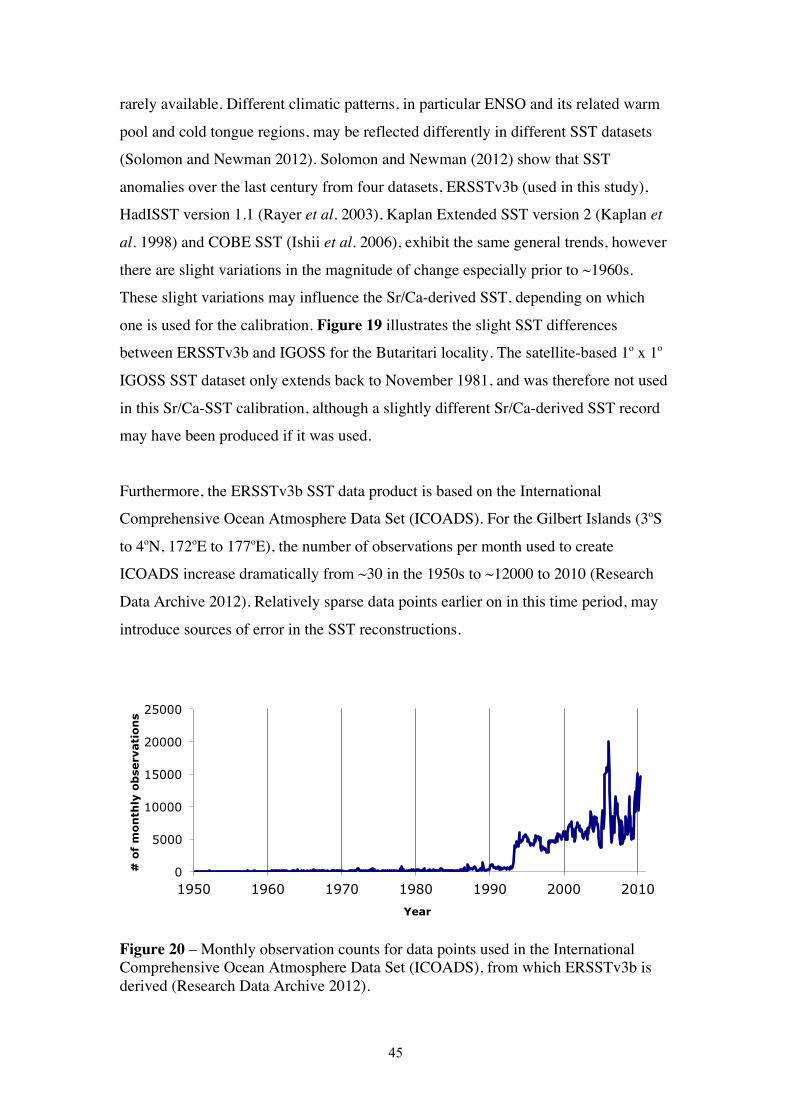
45
rarely available. Different climatic patterns, in particular ENSO and its related warm
pool and cold tongue regions, may be reflected differently in different SST datasets
(Solomon and Newman 2012). Solomon and Newman (2012) show that SST
anomalies over the last century from four datasets, ERSSTv3b (used in this study),
HadISST version 1.1 (Rayer et al. 2003), Kaplan Extended SST version 2 (Kaplan et
al. 1998) and COBE SST (Ishii et al. 2006), exhibit the same general trends, however
there are slight variations in the magnitude of change especially prior to ~1960s.
These slight variations may influence the Sr/Ca-derived SST, depending on which
one is used for the calibration. Figure 19 illustrates the slight SST differences
between ERSSTv3b and IGOSS for the Butaritari locality. The satellite-based 1o x 1o
IGOSS SST dataset only extends back to November 1981, and was therefore not used
in this Sr/Ca-SST calibration, although a slightly different Sr/Ca-derived SST record
may have been produced if it was used.
Furthermore, the ERSSTv3b SST data product is based on the International
Comprehensive Ocean Atmosphere Data Set (ICOADS). For the Gilbert Islands (3oS
to 4oN, 172oE to 177oE), the number of observations per month used to create
ICOADS increase dramatically from ~30 in the 1950s to ~12000 to 2010 (Research
Data Archive 2012). Relatively sparse data points earlier on in this time period, may
introduce sources of error in the SST reconstructions.
Figure 20 – Monthly observation counts for data points used in the International Comprehensive Ocean Atmosphere Data Set (ICOADS), from which ERSSTv3b is derived (Research Data Archive 2012).
0
5000
10000
15000
20000
25000
1950 1960 1970 1980 1990 2000 2010
# o
f m
onth
ly o
bse
rvat
ion
s
Year

46
The bi-monthly resolution of the Sr/Ca record for the Butaritari coral may also be a
limiting factor in the strength of the correlation between Sr/Ca and SST calibration
points. The data at bi-monthly resolution does generally follow the pattern of the
instrumental SST, although there are some differences, especially in the amplitude of
SST change. Increasing the coral dataset to monthly resolution could provide
additional Sr/Ca information, which could further support the current calibration trend
and increase the correlation coefficient, although previous studies have shown that
four to five samples per year, approximately bi-monthly resolution, of skeletal coral
growth can be sufficient for seasonal environmental variability detection (e.g. Aharon
1991; Delaney et al. 1993; Carriquiry et al. 1994). This is also likely true for coral
records from Butaritari. Figure 13 (Section 3.7) shows that SST data from ERSSTv3b
does not change greatly between monthly and bi-monthly resolution. Thus, increasing
the resolution of the coral data to monthly may not provide much new information,
though additional analysis around the maximum and minimum values of each coral
year may help to better constrain these maxima and minima, and improve the Sr/Ca-
SST calibration.
There is a relatively extreme cold temperature point in the late 1960s compared to the
rest of the Sr/Ca values and the corresponding instrumental SST. Figure 19 illustrates
the deviation of this data point from the calibration regression line. The next closest
data point is 0.11 mmol/mol lower than the overall maxima. This equates to a 1.38oC
difference between the overall maxima and the next closest point, based on the Sr/Ca-
SST calibration equation derived for the Butaritari modern coral. This extremely cold
point may well be an outlier, however there are currently no reasons, analytically or
otherwise, to exclude or discount it. According to physical inspection of the relevant
coral ledge and the x-ray (Figure 11, Section 3.2 X-Radiography) there were no
visual abnormalities in the coral material. The laboratory preparation of this sample
was exactly the same as all the other samples. It was run under the same conditions
and on the same ICP-OES machine. The digested Sr/Ca sample solution was analysed
twice, in two separate ICP-OES runs. The resulting Sr/Ca values of 9.25 and 9.23
mol/mol, from which the maxima point was derived, are very similar, suggesting that
this is a real data point.

47
As a result, the extremely cold point has been included in the Sr/Ca-SST and may
very well be a true Sr/Ca value for this coral. The Sr/Ca values presented in this study
are a reflection of the SST in this specific coral, which while they indicate the key
peaks and troughs in the SST record, they can also reflect very localised changes. The
extreme Sr/Ca cold point may just be a reflection of the environmental SST changes
experienced by this coral. Also, despite including a potential ‘outlier,’ the resulting
Sr/Ca-SST calibration equation correlates well with the average published calibration
equation for Porites sp. corals (Corrège 2006). A future recommendation would be to
reprepare and rerun the maxima Sr/Ca sample as well as the samples directly either
side of it from scratch, to further confirm its validity within this Sr/Ca dataset and
Sr/Ca-SST calibration.
5.1.2 Sr/Ca-derived SST
Despite differences, the general amplitudes of change in the Sr/Ca-derived SST and
the SST data product are similar (Figure 19) The mean value and SD for Sr/Ca-
derived SST is 28.83 ± 0.89 oC, and the SST data product is 28.90 ± 0.66 oC. There is
a statistically significant correlation of r = 0.62 (Pearson correlation coefficient)
between these two datasets. (Note same/similar correlation coefficient as for
constructing the coral age model). This suggests that both datasets are successfully
recording the key changes in SST for the area. Consistent with the findings of Mantua
and Hare (2002), an abrupt climatic shift in SST can be identified in the mid-1970s.
The slope of the trends have been calculated using the following standard regression
equation used in Nurhati et al. (2009):
SST = a + m * year
The error of the slope is calculated using the following equations, also used in Nurhati
et al. (2009). The errors reported are solely for the trends.
trend = (m ± $m) * total period of trend (in years)
$trend = $m * total period of trend (in years)

48
Taking Butaritari Sr/Ca-derived SST as an example,
Sr-Ca/derived SST = -1.176 + 0.0151 * Year
trend = (0.0151 ± 0.003) * 51 years
trend = 0.77 oC
$trend = 0.003 * 51 years
$trend = 0.17 oC
There are statistically significant warming trends (p < 0.001) in both the Sr/Ca-SST
and SST data product. The Butaritari coral Sr/Ca-SST record suggests there has been
a 0.77 ± 0.17 oC increase in SST at Butaritari over the 1959 to 2010 period. The SST
data product record suggests that there has been a 0.67 ± 0.12 oC increase in SST over
the 1959 to 2010 period. These suggested warming trends at Butaritari are consistent
with tropical and sub-tropical SST increases of 0.4oC to 1oC estimated from a variety
of data sources over the past 100 years (Deser et al. 2010), and more specifically with
an estimated 0.2oC to 1oC warming of the WP region over the past 50 years (Cravatte
et al. 2009). A further investigation of this warming SST trend is detailed in Section
5.5 through comparison with coral records from the western and central equatorial
Pacific.
5.2 Deciphering SSS from !18O using coral-derived SST
Paired Sr/Ca and !18O coral data is particularly useful in determining the balance of
SSS (and thus the evaporation/precipitation balance) versus SST within a !18O record.
An understanding the SSS balance is important in understanding the climatic
processes that exist at the coral site, such as increases in precipitation in El Niño
years. There are a number of recognised methods to separate the !18Osw signal from
coral !18O. An early method (McCulloch et al. 1994; Gagan et al. 1998) utilises linear
regression equations for coral Sr/Ca-SST and coral !18O-SST in the univariate form of

49
y = mx + c, where y = Sr/Ca or !18O, x = SST, m = regression coefficient and c is
constant. From these equations, coral Sr/Ca and !18O are converted to temperature
units. Through multiplying the slope of the !18O-SST relationship by the difference in
!18O-derived SST and Sr/Ca-derived SST, the residual !18O can be calculated, which
reflects the effects of seawater !18O composition (!18Osw). In an attempt to minimise
error associated with the independent variable (instrumental SST) in the above
method, Ren et al. (2002) proposed a different method, wherein the intercept values
were excluded from the calculation. They determine !18Osw using instantaneous
changes in paired !18O and Sr/Ca, with the following equation:
%!18O(coral) = %!18O(SST contri) + %!18O(sw-contri)
= (#!18O(coral)/#SST) * $SST + (#!18O(coral)/#!18Osw * $!18Osw)
where, $SST = $Sr/Ca(coral)/ (#Sr/Ca(coral)/#SST). %!18OSST is the SST contribution to
coral !18O, and %!18Osw is the !18Osw contribution to coral !18O. #!18O(coral)/#SST and
#!18O(coral)/#!18Osw are the partial derivatives of coral !18O in regard to SST and !18Osw.
#!18O(coral)/#SST and #Sr/Ca(coral)/#SST correspond to the slopes of proxy-SST
regression equations.
Absolute !18Osw values are calculated through summing the instantaneous changes to a
reference salinity value. The reference salinity value is usually derived from
climatological SSS data and/or a !18Osw-SST relationship, such as Fairbanks et al.
(1997), and varies depending on where the coral was collected from (Ren et al. 2002;
Nurhati et al. 2009).
Through comparison of early and Ren et al. (2002) methods, Huppert and Solow 2004
found that the results obtained from each are identical. Furthermore, Cahyarini et al.
(2008) show that their proposed centering method provides the same results as Ren et
al. (2002). Cahyarini et al. (2008) exclude the intercept from their calculation, by
removing the mean from the input variables, termed centering the linear regression
equation (Draper and Smith 1981). The advantage of using the centering method is
that it involves much simplier mathematical calculations than Ren et al. (2002). In

50
this study, !18Osw was derived for the Butaritari coral using the centering method
described in Cahyarini et al. (2008):
%!18Osw-center = (!18Ocorali – mean !18Ocoral) - %1/&1 * (Sr/Cai – mean Sr/Ca)
where, %!18Osw-center is the centered !18Osw contribution to !18O, !18Ocoral is measured
coral !18O, Sr/Ca is measured coral Sr/Ca, mean !18Ocoral and Sr/Ca are the mean
values of the measured respective terms, %1 is the regression slope of coral !18O vs
SST, and &1 is the regression slope of coral Sr/Ca vs SST.
For corals the !18O-SST slope value generally falls within a range of -0.15 to -0.22
‰/oC (Weber and Woodhead 1972; Wellington et al. 1996; Boiseau et al. 1998;
Gagan et al. 1998; Juillet-Leclerc and Schmidt 2001). The %1 value of -0.18 ‰/oC
(Gagan et al. 1998) is considered a reasonable average (Corrège 2006) of published
!18O-SST slopes and was utilised in this study. The &1 value of -0.0688 mmol/mol/ oC
was derived from the regression between Butaritari coral Sr/Ca and ERSSTv3b SST
(see Section 5.2). The mean !18O coral value was -5.20 ‰ and the mean Sr/Ca coral
value was 8.92 mmol/mol. The resulting %!18Osw (Figure 21c) is discussed in the
following section (Section 5.3)
The %!18Osw trend and associated error was calculated using the standard regression
equations from Nurhati et al. (2009) (see Section 5.1.2). The error reported is solely
for the trend, and the calculation is as follows:
%!18Osw = 0.477 - 0.000240 * Year
trend = (0.000240 ± 0.0007) * 51 years
trend = -0.01
$trend = 0.0007 * 51 years
$trend = 0.03 ‰
51
The %!18Osw values at Butaritari do not reflect a statistically significant trend over the
51 year period (-0.01 ± 0.03 ‰; p > 0.001; Figure 21c). A further investigation of
this is detailed in Section 5.5 through comparison with coral records from central
equatorial Pacific.
5.3 Coral geochemistry compared to local climatology
The Butaritari coral geochemistry (Sr/Ca-derived SST and !18O) records show similar
variations to the local climatology of the region (SST and precipitation) and the NINO
4 and SOI ENSO indices (Figure 21). As described in Section 4.1, the Sr/Ca and !18O
reflect very similar patterns, and Sr/Ca and ERSSTv3b SST correlate well with each
other.
Major ENSO events between 1959 and 2010 are predominantly reflected in both the
Sr/Ca-derived SST and !18O Butaritari records, although the relative amplitude of
change does vary from climatological datasets (Figure 21). At Butaritari El Niño
events (SOI < -8 for sustained periods) are visible as minima in Sr/Ca-derived SST
and !18O, warmer SSTs and above average precipitation. In contrast, La Niña events
(SOI > 8 for sustained periods) at Butaritari show Sr/Ca-derived SST and !18O
maxima, and are periods of cooler SST and lower precipitation (Figure 21).
Relative differences between the Sr/Ca-derived SST and !18O exist for the 1987/1988
and ~1991-1995 El Niño years, such that !18O exhibits a relatively larger amplitude
signal in those years compared to Sr/Ca-derived SST (Figure 21). !18O is a function
of both SST and the !18O of seawater (!18Osw), and the larger amplitude !18O signal
may reflect an increase in El Niño-driven precipitation changing the !18Osw in
1987/1988 and 1991-1995.
The relative changes in !18Osw (Figure 21c) visually correlate well to the regions of
greatest difference between !18O and Sr/Ca-derived SST (Figure 21a, b),
predominantly 1965-1982 and 1989-1997. These two periods reflect the freshest

52
periods in the Butaritari record, suggesting that the precipitation influence on !18O is
prominent during these periods. While the generally pattern of !18Osw and
instrumental SSS and precipitation (Figure 21e, f) is somewhat similar, the amplitude
of change does vary. Similar to the variations seen between the Sr/Ca values and
ERSSTv3b SST (see Section 5.1), these differences could be a result of the resolution
of the different records. The coral !18Osw is reflecting very localised changes, whereas
the SSS and precipitation are an average across a larger area.
Butaritari is commonly associated with high precipitation, with an average rainfall
rate of approximately 4 to 8 mm/day (Baker et al. 1994; Xie and Arkin 1996; Xie and
Arkin 1997). These monthly average values depend on the specific precipitation
dataset used. The NOAA NCDC GCPS MONTHLY STATION mean precipitation
(Baker et al. 1994) for 1959 to 1982 is derived from on-site Butaritari measurements
and reflects higher precipitation compared to the 1979 to 2010 monthly CMAP
Estimated Precipitation derived from a 2.5o x 2.5o grid square over Butaritari (Note
precipitation datasets are normalised to unit variance in Figure 21).. Due to the larger
area covered, the CMAP precipitation data may under or over estimate the specific
rainfall at Butaritari. Nonetheless, rainfall still correlates with the ENSO indices
(Figure 21).

53
Figure 21 – Modern Butaritari coral geochemistry compared to local climatology and ENSO indices. a) Butaritari !18O (green). b) Butaritari Sr/Ca-derived SST (red). c) Butaritari %!18Osw (blue). d) SST (red) from ERSSTv3b (Smith et al. 2008) for the 2o x 2o grid square at 2oN, 172oE. The SST dataset has been interpolated to bi-monthly resolution to correspond with the resolution of the coral geochemistry data. e) Normalised mean daily Butaritari precipitation for each month from NOAA NCDC GCPS MONTHLY STATION mean precipitation (Baker et al. 1994) for 1959 to 1982 (light blue) from Butaritari, station ID 9160100, at 3.03N, 172.78E; and monthly CMAP Estimated Precipitation (Xie and Arkin 1996; Xie and Arkin 1997) for 1979 to 2010 (dark blue) for the 2.5o x 2.5o grid square at 1.25N, 171.25W. f) Monthly SSS (at 5.01 meters depth) from CARTON-GIESE SODA latest version (v2p1p6) for the 0.5o

54
x 0.5o grid square at 172.25E 3.25N containing Butaritari Island (Carton and Giese 2008). g) Monthly NINO 4 data (yellow) for the NINO 4 region (5oN-5oS, 160oE-150oW) sourced from http://www.cpc.ncep.noaa.gov. h) Monthly SOI data (pink) sourced from the Australian Bureau of Meteorology (http://www.bom.gov.au/climate/current/soi2.shtml). El Niño threshold (SOI < -8; Australian Bureau of Meteorology 2012a) is marked by a dotted line on the SOI trace. La Niña threshold (SOI > 8) is marked by a dashed line on the SOI trace. El Niño events (SOI < -8 for sustained periods) are shaded dark grey. La Niña events (SOI > 8 for sustained periods) are shaded light grey. Note: inverted y-axes for a), c), f) and h).
Although overall the coral geochemistry and related local climatology corresponds
well with the ENSO indices, the coral signals do appear to be slightly out of synch
with SOI and NINO 4. Some coral peaks (warm and wet periods) seem to appear just
before the SOI and NINO 4 peak events (El Niño periods), suggesting that Butaritari
may experience changes slightly earlier than the ENSO indices indicate. These
differences are noted to occur around 1972-73, 1977, 1986-87, 1991 and 1997 just
before the correspond El Niño periods are evident in the SOI and NINO 4 indices.
Butaritari is located at the equatorial eastern edge of the IPWP, which migrates east-
west as one of the first stages of the development of El Niño events (Picaut et al.
2001). Figure 22 is a modified version of Figure 4 in Section 2.1, and through
highlighting the above years of slight misalignment, illustrates SST and SSS
differences between the EWPCZ migration and SOI. The east-west (El Niño-La Niña)
migration of EWPCZ indicates a slightly greater movement relative to SOI. Taking
1991 as an example, the Butaritari coral Sr/Ca-derived SST and !18O (Figure 21a, b)
show peaks just before the SOI-recognised El Niño period starting in 1992. This early
peak is reflected in the 2o x 2o resolution SST data product (Figure 21c) although not
clearly reflected in the 2.5o x 2.5o resolution precipitation record (Figure 21d). In
1991 (Figure 22) SST shifts in the eastern edge of the IPWP are shown to migrate
further eastward relative to the strength of the SOI. For the same year, SSS is in
relative synch with the SOI. In this way, shifts to warmer SST can be seen to occur
slightly earlier than the in SOI in some years and these appear to be reflected in the
Butaritari coral record. The Butaritari coral is reflecting localised variations in SST
and SSS that may not be recognised to the same extent in the large-scale ENSO
indices, and is thus providing more subtle insights into local ENSO dynamics.

55
Figure 22 – Modified version of Figure 4. Migration of the eastern edge of the
Western Pacific Warm Pool. Left panel is the longitude-time distribution of 4oN-4oS
averaged SST, and the right panel is SSS for the same area. The thick white line is the
Southern Oscillation Index (SOI). Sustained positive and negative SOI correspond to
La Niña and El Niño phases, respectively. Contours are 1oC for SST and 0.25 psu for
SSS. Dark shading in the left and right panels indicates higher SST and higher SSS,
respectively. Orange lines indicate the longitudinal positions of Butaritari Atoll
(~172o30’E, 3o30’N; this study), Tarawa (1oN, 172oE) and Maiana (1oN, 173oE).
(Modified from Picaut et al. 2001). Blue shaded areas correspond to years of slight
misalignment between Butaritari coral and ENSO indices evident in Figure 21).
5.3.1 Wavelet analysis
Wavelet analysis is used to provide a quantification of the visually recognisable
patterns in the data discussed above in Section 5.1. It examines localised variations of
power within a time series (Torrence and Compo 1998). This type of analysis is
effective for analysing time series with multiple timescales and/or changes in variance
(Asami et al. 2005). Wavelet analysis, using the Morlet wavelet was carried out
1991
1986-1987
1977
La Niña !" El Niño

56
through the online Interactive Wavelet Plot (Torrence and Compo 1998), available at
http://paos.colorado.edu/research/wavelets/. Wavelet analysis of Butaritari Sr/Ca-
derived SST and !18O, ERSSTv3b, NINO 4 and SOI further quantifies the dominant
variability in these records and shows that they are influenced by annual, interannual
and decadal variability, albeit in different proportions in each record. All wavelet
analyses in this study have been fitted with a cone of influence (indicated by cross
hatching). This hatched area denotes the region of the wavelet spectrum wherein edge
effects due to finite-length input time series, have had an impact (Torrence and
Compo 1998). These regions have been padded with zeros to reduce edge effects,
however this reduces the amplitude of the variance near the edges, and decreases the
power across the periods near the edges.
• Sr/Ca-derived SST and !18O
The wavelet results for the Butaritari coral Sr/Ca-derived SST and !18O show the
strongest power in the decadal to mutli-decadal periods, though these periods are at
the limit of statistical significance since the Butaritari coral is ~50 years long and
there are only a few realisations of these periods in the record. Figure 23 Part 1
shows a persistent power at the 12-24 year period (multi-decadal variability; coloured
red). Between 1965 and 1984 the cycles of significant power predominantly fall
around periods of 16 to 24 years, and then between 1985 and 2004 the cycles of
significant power predominantly fall around periods of 12 to 16 years. There are some
fluctuations in power at annual periods, though the global wavelet power spectrum
(Figure 23, Part 1c), defined as the time average over the series of wavelet powers
(Ge 2007), suggests this variance is low. There is greater variance in power for the 2-
8 years (interannual) period.
Similar to the !18O, the wavelet results for the Butaritari coral Sr/Ca-derived SST
(Figure 23, Part 2) indicate multi-decadal variability. The time period between 1961
and 1990 sees areas of highest power (although relatively low compared to the other
wavelet results in Figure 24, Figure 25 and Figure 26) in the 24 to 32 year periods.
At 1990 there is a step to variability at decadal periods, which continues through to
2005. A low power annual cycle exists, along with an interannual cycle.
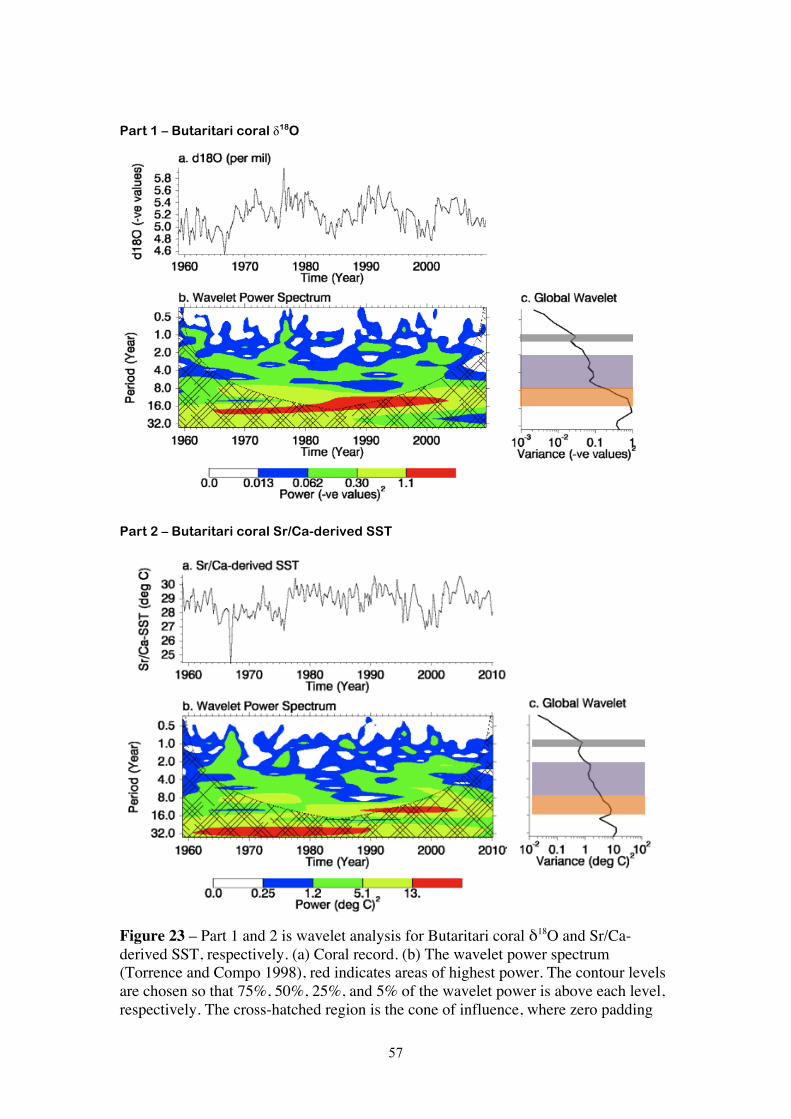
57
Part 1 – Butaritari coral "18O
Part 2 – Butaritari coral Sr/Ca-derived SST
Figure 23 – Part 1 and 2 is wavelet analysis for Butaritari coral !18O and Sr/Ca-derived SST, respectively. (a) Coral record. (b) The wavelet power spectrum (Torrence and Compo 1998), red indicates areas of highest power. The contour levels are chosen so that 75%, 50%, 25%, and 5% of the wavelet power is above each level, respectively. The cross-hatched region is the cone of influence, where zero padding

58
has reduced the variance. (c) The global wavelet power spectrum, which is the average variance of each period for the whole time series. Grey shading corresponds to annual variance; purple shading corresponds to interannual (2-8 years) variance; and orange shading corresponds to ~decadal variance.
• ENSO indices and SST
As expected, the wavelet analysis of the ENSO indices, NINO 4 and SOI, show
dominant interannual cycles throughout the 1959 to 2010 time period. These
interannual cycles correspond directly to interannual ENSO events, which the NINO
4 and SOI indices are designed to represent. The NINO 4 anomaly (Figure 24)
indicates high power interannual cycles (2-8 years) across the record, especially
around 1970 and 1985-1990. The SOI results (Figure 25) reflects a similar pattern to
NINO 4. Both records also include high power near-decadal variance pattern between
1970 and 2005, along with a low power annual cycle.
The SST product wavelet analysis (Figure 26) indicates a prominent near-decadal
variance, similar to the coral proxies. A medium power interannual cycle can be
identified as well as a lower power annual cycle.

59
Figure 24 – (a) NINO4 anomaly. (b) The wavelet power spectrum (Torrence and Compo 1998), red indicates areas of highest power. The contour levels are chosen so that 75%, 50%, 25%, and 5% of the wavelet power is above each level, respectively. The cross-hatched region is the cone of influence, where zero padding has reduced the variance. (c) The global wavelet power spectrum, which is the average variance of each period for the whole time series. Grey shading corresponds to annual variance; purple shading corresponds to interannual (2-8 years) variance; and orange shading corresponds to ~decadal variance.
Figure 25 – (a) SOI. (b) The wavelet power spectrum (Torrence and Compo 1998), red indicates areas of highest power. The contour levels are chosen so that 75%, 50%, 25%, and 5% of the wavelet power is above each level, respectively. The cross-hatched region is the cone of influence, where zero padding has reduced the variance. (c) The global wavelet power spectrum, which is the average variance of each period for the whole time series. Grey shading corresponds to annual variance; purple shading corresponds to interannual (2-8 years) variance; and orange shading corresponds to ~decadal variance.

60
Figure 26 – (a) SST (ERSSTv3b; Smith et al. 2008). (b) The wavelet power spectrum (Torrence and Compo 1998), red indicates areas of highest power. The contour levels are chosen so that 75%, 50%, 25%, and 5% of the wavelet power is above each level, respectively. The cross-hatched region is the cone of influence, where zero padding has reduced the variance. (c) The global wavelet power spectrum, which is the average variance of each period for the whole time series. Grey shading corresponds to annual variance; purple shading corresponds to interannual (2-8 years) variance; and orange shading corresponds to ~decadal variance. Overall the wavelet analysis results reveal a persistent decadal and/or multi-decadal
pattern within the Butaritari coral Sr/Ca-derived SST and !18O, and in the
instrumental SST. Interannual variability is present in these three records, but in the
SOI and NINO 4 records interannual variability dominates. The decadal variations
evident in the ~50 year Butaritari coral record are in line with the observational
findings of Wang and Mehta (2008). In their explorative study of decadal variability
of the IPWP, significantly strong peaks (9.7 year) were revealed in a power spectrum
analysis of a 50 year (1952-2001) record of instrumental SST, and atmospheric and
oceanic reanalyses. Decadal variation in the IPWP may be influenced by the Pacific
Decadal Oscillation (PDO). A positive PDO can enlarge the IPWP at both seasonal
and decadal time scales (Bolan and Lixin 2012), and this warm pool enlargement
during these periods may be influencing the Butaritari signal. In spite of this however,
Newman et al. (2003) conclude that PDO is dependent upon ENSO on all timescales,

61
and hence ENSO maintains a prominent influence over the climatic variability in this
region.
It is however, somewhat challenging to infer decadal or larger patterns within a 50
year record, as is the case for the Butaritari coral and SST records, since even one 10
year oscillation covers one fifth of the available data. A data record of 100 years or
more would provide greater information about the frequency and amplitude of these
~10 year cycles. The decadal and multi-decadal variance evident in the wavelet
analysis of the 50 year-long Butaritari record, suggest that a longer coral time series
record is needed to define this variance.
Although differences in the variance patterns do occur between the instrumental and
coral records, the 50-year Butaritari coral reflects the climatic variance changes of the
region (comparison with SST), and of the broader tropical Pacific processes (SOI,
NINO 4) at the decadal/multi-decadal and interannual periods. Thus the Butaritari
coral record can be used to investigate the climate dynamics of the eastern edge of the
warm pool.
5.4 Butaritari compared to Tarawa and Maiana
Similar to Nurhati et al. (2009) wherein Sr/Ca and !18O coral records from several
closely situated central tropical Pacific islands were examined for spatial variability,
the geochemical results from this Butaritari study are compared with those from other
nearby sites to gain a broader understanding of the climatological forces at work in
the western equatorial Pacific region.
!18O data from Tarawa located directly due south of Butaritari (1oN, 172oE) (Cole et
al. 1993) and Maiana located south-south-east of Butaritari (1oN, 173oE) (Urban et al.
2000) were compared to the !18O Butaritari data (3o30’N, 172o30’E). Including
Butaritari, these three neighbouring islands are located in the Gilbert Island group of
Kiribati, and are situated along a known precipitation gradient and along the salinity

62
front at the eastern edge of the IPWP. ENSO variability is recorded at all three sites
(Cole et al. 1993; Urban et al. 2000; this study see Section 5.3).
The complete dataset for Tarawa (1894-1990; monthly resolution) was smoothed
using a 24 point moving average. Maiana (1840-1994; bi-monthly resolution) and
Butaritari (1959-2010; bi-monthly resolution) data was smoothed using a 12 point
moving average. This smoothing removed all < 2 year signals, so that a comparison
between interannual signals, primarily ENSO, and decadal signals could be made
(Figure 27a). The Maiana !18O is the longest record of the three examined and
extends furthest back in time to 1840. The Butaritari !18O record from this study
covers the period between 1959 and 2010, and hence the other two datasets were
truncated to this ~50 year period of overlap with the Butaritari record (Figure 27b).
Figure 27 – Coral !18O records from three western equatorial Pacific islands. A) 1840 to 2000. Green dotted line corresponds to bi-monthly Butaritari (3o30’N, 172o30’E ) !18O data from this study. Blue dotted line corresponds to monthly Tarawa (1oN, 172oE) !18O data from Cole et al. (1993). Red dotted line corresponds to bi-monthly Maiana (1oN, 173oE) !18O data from Urban et al. (2000). Solid lines correspond to moving averages (12 point for Butaritari and Maiana, and 24 point for Tarawa), which remove < 2 year variability from the data. Black bracket indicates the area of overlap with the Butaritari record. B) Same as for A) except for 1959 to 2000, the area of

63
overlap with the Butaritari record. Monthly SOI data (pink) sourced from the Australian Bureau of Meteorology (http://www.bom.gov.au/climate/current/soi2.shtml). El Niño threshold (SOI < -8) is marked by a dotted line on the SOI trace. La Niña threshold (SOI > 8) is marked by a dashed line on the SOI trace. El Niño events (SOI < -8 for sustained periods) are shaded dark grey. La Niña events (SOI > 8 for sustained periods) are shaded light grey.
Visual comparison of the moving average data in Figure 27b, suggests that with the
~annual signals removed, Butaritari, Tarawa and Maiana reflect somewhat similar
patterns of peaks and troughs across the overlapping time interval, although the
consistently more negative !18O values show that Butaritari is warmer and wetter than
both Tarawa and Maiana.
The Tarawa moving average data were interpolated using ARAND software (Howell
et al. 2006) from monthly to bi-monthly resolution to enable a linear regression
between datasets to be undertaken. Through regression the Pearson correlation
coefficient between Butaritari and Tarawa was found to be r = 0.008, indicating very
weak or no correlation. The correlation relationship between Butaritari and Tarawa is
not statistically significant (p > 0.001). The Pearson correlation coefficient between
Butaritari and Maiana is r = 0.56, indicating a moderate correlation. This relationship
is statistically significant (p < 0.001). The Tarawa record sits between Butaritari
(warmer, wetter) and Maiana (colder, drier) and appears to follow a more similar
pattern to Maiana than Butaritari. The correlation is good between Tarawa and
Maiana, r = 0.72 (p < 0.001). The fact that Tarawa and Maiana are more correlated
with each other than they are with Butaritari is interesting as it they are situated at the
same latitude, only 1o of longitude apart. Butaritari and Tarawa are at the same
longitude, only 1o of latitude apart. This suggests that there is more of a latitudinal
variation (north-south) than longitudinal variation (east-west) in !18O for these three
neighbouring islands.
As discussed earlier in Section 5.1, a decadal and/or multi-decadal pattern appears to
exist within the 50 year Butaritari coral record. Wavelet analysis of Tarawa and
Maiana !18O data for the period of overlap with the Butaritari record, suggest that
decadal to multi-decadal patterns also exist at these neighbouring locations. Tarawa

64
!18O exhibits a decadal and/or multi-decadal period throughout the whole record,
though the record is dominated by variance around 2 to 8 years, corresponding to
interannual ENSO-related variation, particularly between 1965 and 1975 (Figure 28).
This is consistent with the interannual frequency periods identified for Tarawa
through spectral analysis by Cole et al. (1993). Maiana exhibits some lower power
interannual (2 to 8 year) variability compared to Tarawa (though the interannual
variance still dominates the record), and some lower power decadal patterns and a
signal at a ~32 year period (Figure 29). When the wavelet results for all three islands
are taken together, Butaritari shows the strongest near-decadal oscillations (Figure 23). It must be noted however, the Tarawa record used for wavelet analysis was only
31 years in length between 1959 and 1990. The Maiana record was 35 years in length
between 1959 and 1994. Therefore, the decadal and/or multi-decadal patterns must be
taken with caution, as the time period for analysis is quite short, and the results may
vary significantly if longer records are used for wavelet analysis.
Figure 28 – (a) Tarawa !18O for the period of overlap with the Butaritari record. (b) The wavelet power spectrum (Torrence and Compo 1998), red indicates areas of highest power. The contour levels are chosen so that 75%, 50%, 25%, and 5% of the wavelet power is above each level, respectively. The cross-hatched region is the cone of influence, where zero padding has reduced the variance. (c) The global wavelet power spectrum, which is the average variance of each period for the whole time series. Grey shading corresponds to annual variance; purple shading corresponds to

65
interannual (2-8 years) variance; and orange shading corresponds to ~decadal variance.
Figure 29 – (a) Maiana !18O for the period of overlap with the Butaritari record. (b) The wavelet power spectrum (Torrence and Compo 1998), red indicates areas of highest power. The contour levels are chosen so that 75%, 50%, 25%, and 5% of the wavelet power is above each level, respectively. The cross-hatched region is the cone of influence, where zero padding has reduced the variance. (c) The global wavelet power spectrum, which is the average variance of each period for the whole time series. Grey shading corresponds to annual variance; purple shading corresponds to interannual (2-8 years) variance; and orange shading corresponds to ~decadal variance.
Between 1959 and 2010 the mean !18O value for Butaritari is -5.20 ‰. Between 1959
and 1990 the mean !18O value for Tarawa is -4.90 ‰. Between 1959 and 1994 the
mean !18O value for Maiana is -4.67 ‰. The differences in the mean !18O in the three
records (averaged over the overlapping intervals with Butartari, 1959 to 1990 for
Tarawa and 1959 to 1994 for Maiana) appear to correlate with the geographical
positions of each island (Figure 27). Butaritari is the most northern of the three
islands, located at 3o30’N, 172o30’E, and indicates the warmest/wettest !18O signal.
The precipitation instrumental record (Figure 30) supports a north-south rainfall
gradient between Butaritari (3o30’N) and Tarawa and Maiana (1oN). According to
Figure 30, Tarawa and Maiana experience the same levels of rainfall, which suggests

66
the differences between the Tarawa and Maiana !18O signals are not primarily due to
changes in precipitation. The IGOSS SST data product indicates a similar pattern to
precipitation however there appears to be a slight difference in SST between Tarawa
and Maiana even though they are on the same latitude (Figure 31). Tarawa is closer
to the 29oC contour line than Maiana. Correspondingly, the !18O signal is more
positive at Maiana, indicating cooler SST. The differences between Tarawa and
Maiana appear to be driven mostly be temperature. This small east-west SST
difference may be attributed to the fluctuations in the convergence of the western and
central equatorial water bodies along the eastern edge of the IPWP.
"
Figure 30 – Zoomed in section of Figure 8. Mean precipitation data for the time period between January 1979 to November 2011 derived from CMAP Precipitation data from NOAA NCEP CPC Merged Analysis monthly latest version 1 precipitation estimate (Xie and Arkin 1996; Xie and Arkin 1997). The location of Butaritari (this study; 3o30’N, 172o30’E) is indicated by a yellow circle. The locations of Tarawa (1oN, 172oE) and Maiana (1oN, 173oE) are indicated by a red square and purple star respectively. Central Pacific islands: Palmyra (blue rectangle; 6oN, 162oW), Fanning (black rectangle; 4oN, 159oW) and Christmas (orange rectangle; 2oN, 157oW).

67
" "
Figure 31 – Zoomed in section of (Figure 7). Mean monthly SST for the time period between 1959 to 2010 derived from ERSSTv3b (Smith et al. 2008). Black contours = 0.5oC. The location of Butaritari (this study; 3o30’N, 172o30’E) is indicated by a yellow circle. The locations of Tarawa (1oN, 172oE) and Maiana (1oN, 173oE) are indicated by a black square and purple star respectively. Central Pacific islands: Palmyra (blue rectangle; 6oN, 162oW), Fanning (black rectangle; 4oN, 159oW) and Christmas (orange rectangle; 2oN, 157oW).
Figure 32 – !18O records and trend lines for Butaritari (green), Tarawa (blue) and Maiana (red). The Tarawa and Maiana data are from longer datasets however they have been truncated to the period of overlap with the Butaritari record (see Figure 27). The black bracket indicates the common interval between all three datasets.
68
Using the same methods as in Section 5.2.2, the slope of the trend for Butaritari !18O
(1959-2010) is,
!18O = 1.104 - 0.00318 * Year
trend = (-0.00318 ± 0.0009) * 51 years
trend = -0.16 ‰
$trend = 0.0009 * 51 years
$trend = 0.04 ‰
All three islands !18O records reflect statistically significant trends over the common
data interval (1959-1990) towards depleted !18O values, which reflect trends in
combined warming and/or freshening (p < 0.001) (Figure 32; Table 3). The greatest
trend is evident at Maiana and the smallest trend is evident at Tarawa, although the
Tarawa and Butaritari trends are very similar. The !18O Butaritari record suggests a
combined warming and freshening trend of -0.28 ± 0.06 ‰ over 31 years between
1959 and 1990. The !18O Tarawa record indicates a trend of -0.23 ± 0.03 ‰ over the
same time period, and the !18O Maiana record suggests a trend of -0.49 ± 0.05 ‰
over the same time period. The differences in these trends between the neighbouring
islands imply that despite the relatively close distances between them, each island
experiences localised variations in !18O. !18O is a function of both localised SST
and/or SSS, which is primarily influenced by precipitation/evaporation. Move
negative !18O values correspond to warmer and wetter conditions. Apart from the
Butaritari coral, which has paired Sr/Ca and !18O, the !18O for Tarawa and Maiana
cannot be separated into its components parts, SST and SSS. Taken together however,
these three corals suggest significant warming and/or freshening trends over the
common data interval (1959-1990) that increase both towards the equator and in an
easterly direction.
The overall trend in the full Butaritari record (1959-2010) reflects a slightly lower yet
still significant warming and/or freshening pattern, compared to the 1959-1990 period
for the same coral (Table 3). The Maiana record (1959-1994 for the period of overlap

69
with the Butaritari coral) reflects a slightly higher yet still statistically significant
warming and /or freshening trend, compared to the 1959-1990 period.
Table 3 - !18O trends in Butaritari (this study), Tarawa (Cole et al. 1993) and Maiana (Urban et al. 2000) for the common data interval (1959-1990) and overall (1959-2010 for Butaritari and 1959-1994 for Maiana). Island Location Trend in
common interval (1959-1990)
Length of trend period (years)
Significance Trend overall
Length of trend period (years)
Significance
Butaritari 3o30’N, 172o30’E
-0.28 ± 0.06 ‰ 31 p < 0.001 -0.16 ± 0.04 ‰ *for 1959-2010
51 p < 0.001
Tarawa 1oN, 172oE
-0.23 ± 0.03 ‰ 31 p < 0.001 Same as common interval trend
Maiana 1oN, 173oE
-0.49 ± 0.05 ‰ 31 p < 0.001 -0.55 ± 0.05 ‰ *for 1959-1994
35 p < 0.001
5.5 Butaritari compared to other Pacific records
A significant late 20th century warming and freshening trend has also been observed
in paired coral !18O and Sr/Ca records from Palmyra, Fanning and Christmas Islands
(2oN-6oN, 157oW-162oW) in the central equatorial Pacific (Figure 33b; Nurhati et al
2009). These islands are part of the Line Island group of Kiribati and are located at
similar latitudes to Butartari, Tarawa and Maiana in the western equatorial Pacific
(Figure 30, 31). !18O records from all six islands suggest similar freshening and
warming trends (Figure 33) and show interannual variability related to ENSO. El Niño
and La Niña signals reflected in the SOI are evident in all coral records, albeit in
varying degrees. Additional coral data from Christmas Island (Evans et al. 1998;
McGregor et al. 2011) has been plotted on the following figures to provide a visual
representation of a longer dataset for Christmas. It must be noted however, that only
the Nurhati et al. (2009) trends are compared with western Pacific corals. It also must
be noted that the trends reported by Nurhati et al. (2009) include estimates of the total
error. The Butaritari trends include estimates of the trend slope error, one component

70
of the total error. Despite differences in the error estimates, the relative trends
indicated at each locality can be compared to each other.
The western Pacific corals from Butaritari, Tarawa and Maiana indicate a combined
freshening and/or warming overall trend of between -0.16 and -0.55 ‰ (Figure 33a;
see Section 5.4). However, for the period of overlap with the central Pacific corals
(1972-1998), Butaritari exhibits no statistically significant warmer or freshening trend
(0.06 ± 0.05 ‰, p > 0.001). The Tarawa and Maiana records indicate warming and/or
freshening trends (p < 0.001), however due to the limits of the coral records, they do
not span the full overlapping period (1972-1998) with Nurhati et al. (2009), and
therefore the trends cannot be compare on equal terms. In comparison to the Butaritari
insignificant trend, the central Pacific corals from Pamlyra, Fanning and Christmas
suggest a combined freshening and/or warming of between -0.32 and -0.52 ‰ (Figure
33b; Nurhati et al. 2009).
Table 4 - Butaritari (this study), Tarawa (Cole et al. 1993) and Maiana (Urban et al. 2000), Palmyra, Fanning and Christmas (Nurhati et al. 2009) !18O trends. Island Location( Trend overlapping period
(1972-1998)
Length of
trend period
(years)
Significance
Butaritari 3o30’N, 172o30’E 0.06 ± 0.05 ‰ 26 p > 0.001
Tarawa 1oN, 172oE -0.28 ± 0.04 ‰ *for 1972-1990 18 p < 0.001
Maiana 1oN, 173oE -0.26 ± 0.06 ‰ *for 1972-1994 22 p < 0.001
Palmyra 6oN, 162oW -0.52 ± 0.09 ‰ 26 p < 0.001
Fanning 4oN, 159oW -0.40 ± 0.09 ‰ 26 p < 0.001
Christmas 2oN, 157oW -0.32 ± 0.10 ‰ 26 p < 0.001
There appears to be a slightly smaller relative gradient between trends in the central
Pacific coral records compared to the western Pacific corals (Figure 33). There is a
greater gradient difference between corals that are closer together (i.e. Butaritari,
Tarawa and Maiana) than in corals that are a few more degrees of latitude and
longitude apart (Palmyra, Fanning and Christmas). This may indicate that there may
be more climate variability in the western equatorial Pacific, although the forces
driving the variability are slightly different, for example the eastern edge of the IPWP
in the west fluctuates significantly during ENSO events, which may have a more

71
pronounced impact on those islands in the west, through increased advection and
rainfall from warmer SST.
There appears to be the same geographical gradient in both central and western
Pacific, wherein more negative !18O values are given by the islands located furthest
north (Butaritari in the west and Palmyra and Fanning in the central). This may be a
result of the impact of the ITCZ, which brings substantial rainfall (and thus a decrease
in SSS) to the northern islands (Nurhati et al. 2009).
Figure 33 – Coral !18O records from three western (a) and three central (b) equatorial Pacific islands. a) !18O records from Butaritari (green line; bi-monthly resolution; 3o30’N, 172o30’E; this study), Tarawa (blue line; monthly resolution; 1oN, 172oE; Cole et al. 1993) and Maiana (red line; bi-monthly resolution; 1oN, 173oE; Urban et al. 2000) islands between 1959 and 1990. b) !18O records from Palmyra (pink line; monthly resolution; 6oN, 162oW; Cobb et al. 2001), Fanning (black line; monthly resolution; 4oN, 159oW; Nurhati et al. 2009) and Christmas (orange line; monthly resolution; 2oN, 157oW; Nurhati et al. 2009) islands between 1972 and 1998; Christmas between 1959 and 1993 (Evans et al. 1998), and between 1978 and 2007 (McGregor et al. 2011). c) Monthly Southern Oscillation Index (SOI) available from the Australian Bureau of Meteorology (http://www.bom.gov.au/climate/current/soi2.shtml). El Niño threshold (SOI < -8) is marked by a dotted line on the SOI trace. La Niña threshold (SOI > 8) is marked by a dashed line on the SOI trace. The black bracket indicates the common interval between datasets (1972-1998).

72
The Butaritari Sr/Ca-derived SST record reveals a significant warming trend of 0.77 ±
0.17 oC between 1959 and 2010 (Figure 34a; see Section 5.1). For the period
corresponding with the Nurhati et al. (2009) data, Butaritari exhibits an identical
significant warming trend of 0.77 ± 0.15 oC. Palmyra, Fanning and Christmas also
reveal significant warming trends, 0.94 ± 5.81 oC, 1.37 ± 06.57 oC and 1.65 ± 5.73 oC,
respectively, between 1972 and 1998 (Table 5, Figure 34b; Nurhati et al. 2009). The
trends between the western and central Pacific are similar, although more warming
appears to occur in the central Pacific corals.
Table 5 - Butaritari (this study), Palmyra, Fanning and Christmas (Nurhati et al. 2009) Sr/Ca-SST trends. !<=*0D( Location( E+-0D(47-+=*))/01(
)-+/4D(@FG>H$FGGIA(
Length of
trend period
(years)(
'/10/9/2*02-(
H8A-&5A-&5! 3o30’N, 172o30’E! >(NN!O!>('2!#P! )G! =!Q!>(>>'!
"-,/:&-! 6oN, 162oW! >(MD!O!2(L'!#P! )G! =!Q!>(>>'!
E-66560! 4oN, 159oW! '(CN!O!G(2N!#P! )G! =!Q!>(>>'!
PR&5.A/-.! 2oN, 157oW! '(G2!O!2(NC!#P! )G! =!Q!>(>>'!

73
Figure 34 – Coral Sr/Ca-derived SST records from one western (a) and three central (b) equatorial Pacific islands. a) Sr/Ca-derived SST record from Butaritari (green line; bi-monthly resolution; 3o30’N, 172o30’E; this study) between 1959 and 1990. b) Sr/Ca-derived SST records from Palmyra (pink line; monthly resolution; 6oN, 162oW; Cobb et al. 2001), Fanning (black line; monthly resolution; 4oN, 159oW; Nurhati et al. 2009) and Christmas (orange line; monthly resolution; 2oN, 157oW; Nurhati et al. 2009) islands between 1972 and 1998. c) Monthly Southern Oscillation Index (SOI) as described in Figure 33. The black bracket indicates the common interval between datasets (1972-1998).
The !18Osw values for Palmyra, Fanning and Christmas Islands (Nurhati et al. 2009)
were calculated using the Ren et al. (2002) method. As discussed earlier in Section
5.3, Cahyarini et al. (2008) found that the their proposed centering method for
determining !18Osw produces the same results as the Ren et al. (2002), except Ren et
al. (2002) go one step further and calculate the cumulative contributions of !18Osw to
an arbitrary reference. To make the results from both methods directly comparable,
the mean reconstructed !18Osw value calculated using the Ren et al. (2002) method in
Nurhati et al. (2009) is subtracted from reconstructed !18Osw. This provides the
relative variations in !18Osw (Cahyarini et al. 2008). Removing the mean reconstructed
!18Osw from each reconstructed !18Osw value does not alter the trend, and thus any
trends evident from Butaritari and the three central Pacific corals can be compared on
common terms.
Table 6 - Butaritari (this study), Palmyra, Fanning and Christmas (Nurhati et al. 2009) !18Osw trends. !<=*0D( Location( E+-0D(47-+=*))/01(
)-+/4D(@FG>H$FGGIA(
Length of
trend period
(years)(
'/10/9/2*02-(
H8A-&5A-&5! 3o30’N, 172o30’E! >('2!O!>(>2!S! )G! =!T!>(>>'!
"-,/:&-! 6oN, 162oW! K>(C)!O!>(>L!S! )G! =!Q!>(>>'!
E-66560! 4oN, 159oW! K>(')!O!>(>L!S! )G! =!Q!>(>>'!
PR&5.A/-.! 2oN, 157oW! >(>C!O!>(''!S! )G! =!T!>(>>'!
The !18Osw record from Butaritari exhibits no statistically significant trends over the
51 year period between 1959 and 2010 (-0.01 ± 0.03 ‰; p > 0.001, Section 5.2), nor
over the period of comparison with Nurhati et al. (2009), 0.15 ± 0.05 ‰ (p > 0.001).
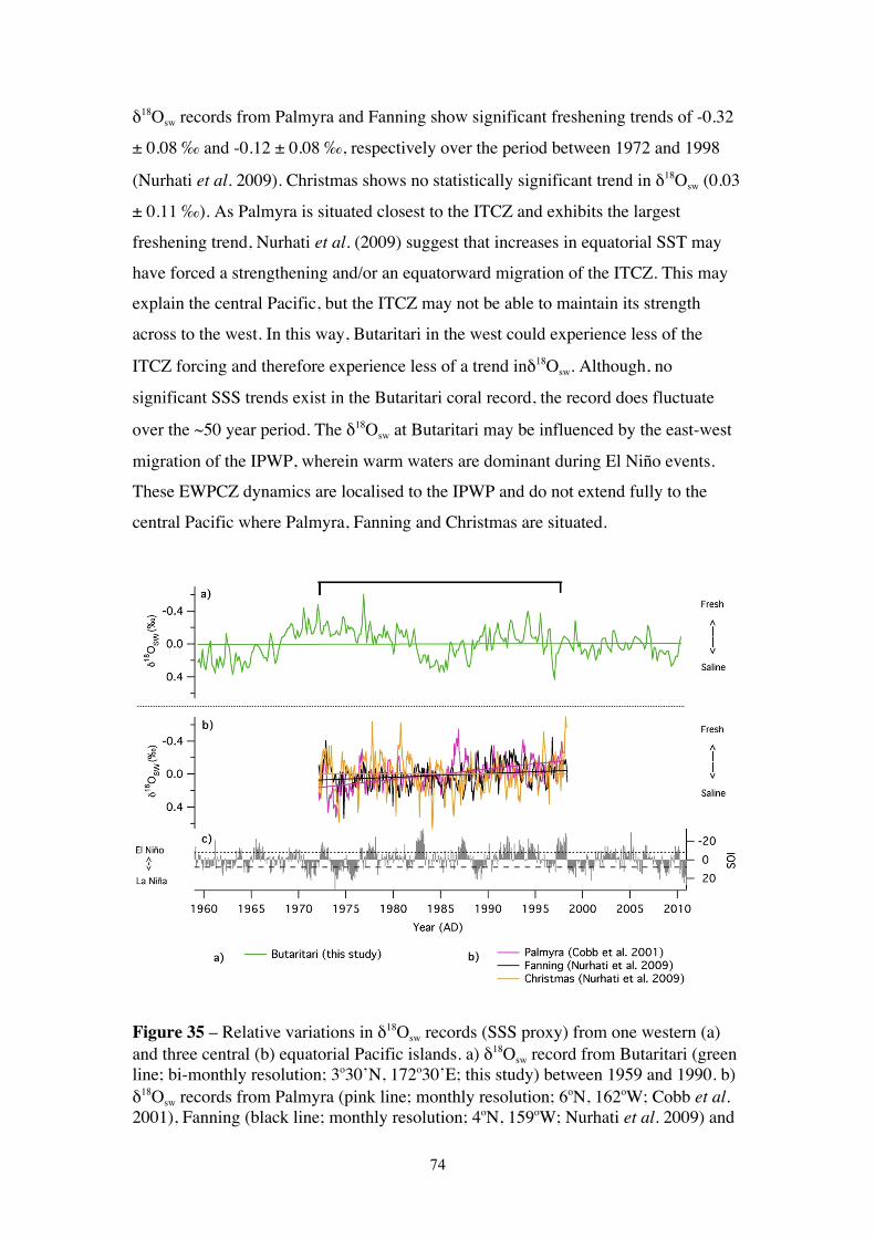
74
!18Osw records from Palmyra and Fanning show significant freshening trends of -0.32
± 0.08 ‰ and -0.12 ± 0.08 ‰, respectively over the period between 1972 and 1998
(Nurhati et al. 2009). Christmas shows no statistically significant trend in !18Osw (0.03
± 0.11 ‰). As Palmyra is situated closest to the ITCZ and exhibits the largest
freshening trend, Nurhati et al. (2009) suggest that increases in equatorial SST may
have forced a strengthening and/or an equatorward migration of the ITCZ. This may
explain the central Pacific, but the ITCZ may not be able to maintain its strength
across to the west. In this way, Butaritari in the west could experience less of the
ITCZ forcing and therefore experience less of a trend in!18Osw. Although, no
significant SSS trends exist in the Butaritari coral record, the record does fluctuate
over the ~50 year period. The !18Osw at Butaritari may be influenced by the east-west
migration of the IPWP, wherein warm waters are dominant during El Niño events.
These EWPCZ dynamics are localised to the IPWP and do not extend fully to the
central Pacific where Palmyra, Fanning and Christmas are situated.
Figure 35 – Relative variations in !18Osw records (SSS proxy) from one western (a) and three central (b) equatorial Pacific islands. a) !18Osw record from Butaritari (green line; bi-monthly resolution; 3o30’N, 172o30’E; this study) between 1959 and 1990. b) !18Osw records from Palmyra (pink line; monthly resolution; 6oN, 162oW; Cobb et al. 2001), Fanning (black line; monthly resolution; 4oN, 159oW; Nurhati et al. 2009) and

75
Christmas (orange line; monthly resolution; 2oN, 157oW; Nurhati et al. 2009) islands between 1972 and 1998. c) Monthly Southern Oscillation Index (SOI) as described in Figure 33.
CONCLUSIONS AND RECOMMENDATIONS
This project aimed to investigate the climatic variability of the western equatorial
Pacific, with particular reference to ENSO. Paired Sr/Ca and !18O were measured
from a Butaritari coral core, and coral-specific SST and !18Osw were calculated,
respectively. The Butaritari coral records correlate well with local climatology (SST,
precipitation and SSS), and the applicable ENSO indices, NINO 4 and SOI. Wavelet
analysis indicates similar interannual, decadal and/or multi-decadal between data
across the ~50 year time period. The Butaritari coral-derived SST exhibits a warming
trend over the ~50 year period that is consistent with instrumental data products in
both the IPWP and Pacific-wide basin, and coral records from the central Pacific. The
!18O trend indicates a combined warming and/or freshening, while no significant
trends have been identified within the !18Osw component over the past 50 years. These
results have been compared to corals from nearby Tarawa and Maiana and central
equatorial Pacific islands.
Recommendations for future work related to this study:
K Measure the geochemistry in a second, potentially longer modern coral
from the Butaritari locality to verify the results found in this study, in
particular the Sr-Ca-SST calibration.
K Analyse the entire Butaritari modern coral core. This study investigated
the time period ~1960 and 2010, however the coral core extends back to at
approximately 1948/1950. An additional decade worth of geochemistry
data could be useful in further exploring the patterns and trends evident in
the current analysis.

76
K Further comparisons of the trends evident at Butaritari with other
equatorial Pacific coral records such as those from Nauru (0o30’S, 166oE)
(Guilderson and Schrag 1999), and Madang, Papua New Guinea (5o13’ S,
145o49’E) (Tudhope et al. 1995), over longer long periods.
K Investigate the geochemical signals of fossil coral cores collected from
Butaritari Atoll. Well preserved fossil corals from the tropical Pacific can
act as very useful archives of past climates as they extend beyond the
limited modern instrumental data. Reliable instrumental SST data for this
tropical region rarely extends beyond 1950 (Gagan et al. 2000). Fossil
coral corks and cores were collected from Butaritari in May 2010 and
August 2011, respectively. Some of these samples have been preliminarily
dated to have ages circa 1500 to 1600 AD. These ages correspond to a
period known as the ‘Little Ice Age’, wherein ENSO is thought to be
influenced by small fluctuations in the extent of incoming solar radiation
(Cobb et al. 2003). Preliminary preservation checks (x-ray diffraction and
thin section analysis) of one fossil core have indicated potential suitability
for high resolution geochemical analysis, especially !18O. A comparison
could be made between the Butaritari modern coral-derived climate
records and the fossil corals, and the evolution of ENSO could be further
explored.
!
The results of this study are significant as they establish Butaritari Atoll as a useful
site for coral climate reconstructions, particularly at the dynamic equatorial eastern
edge of the IPWP.

77

78
REFERENCES Abram, N. J., McGregor, H. V., Gagan, M. K., Hantoro, W. S. and Surwargadi, B. W.
(2009). 'Oscillations in the southern extent of the Indo-Pacific Warm Pool during the mid-Holocene.' Quaternary Science Reviews, 28: 2794-2803.
Aharon, P. (1991). 'Recorders of reef environment histories: Stable isotopes in corals, gaint clams, and calcareous algae.' Coral Reefs, 10: 71-90.
Alibert, C. and McCulloch, M. T. (1997). 'Strontium/calcium ratios in modern Porites corals from the Great Barrier Reef as a proxy for sea surface temperature: Calibration of the thermometer and monitoring of ENSO.' Paleoceanography, 12: 345-363.
Allison, N. and Finch, A. A. (2004). 'High-resolution Sr/Ca records in modern Porites lobata corals: effects of skeletal extension rate and architecture.' Geochemistry, Geophysics, Geosystems, 5: Q05001.
Asami, R., Yamada, T. and Yasufumi, I. (2005). 'Interannual and decadal variability of the western Pacific sea surface condition for the years 1787–2000: Reconstruction based on stable isotope record from a Guam coral.' Journal of Geophysical Research, 110: C05018.
Australian Bureau of Meteorology (2012a). Climate Glossary - Southern Oscillation Indiex (SOI). Accessed 20/06/2012, http://www.bom.gov.au/climate/glossary/soi.shtml.
Australian Bureau of Meteorology (2012b). About ENSO monitoring graphs. Accessed 26/06/2012, http://www.bom.gov.au/climate/enso/indices/about.shtml.
Australian Bureau of Meteorology and CSIRO (2011). Climate Change in the Pacific: Scientific Assessment and New Research - Chapter 6 Kiribati. Volume 2: Country Reports. Accessed 30/04/2012, http://www.cawcr.gov.au/projects/PCCSP/Nov/Vol2_Ch6_Kiribati.pdf.
Baker, C. B., Eischeid, J. K., Karl, T. R. and Diaz, H. F. (1994). 'The quality control of long-term climatological data using objective data analysis.' Preprints of AMS Ninth Conference on Applied Climatology, Dallas, TX.
Beck, J. W., Edwards, R. L., Ito, E., Taylor, F. W., Recy, J., Rougerie, F., Joannot, P. and Henin, C. (1992). 'Sea-surface temperature from coral skeletal strontium/calcium ratios.' Science, 257: 644-647.

79
Bjerknes, J. (1969). 'Atmospheric teleconnections from the equatorial Pacific.' Monthly Weather Review, 97,(3): 163-172.
Boiseau, M., Juillet-Leclerc, A., Yiou, P., Salvat, B., Isdale, P. and Guillaume, M. (1998). 'Atmospheric and oceanic evidences of El Nifio-Southern Oscillation events in the south central Pacific Ocean from coral stable isotopicrecordsover the last 137 years.' Paleoceanography, 13,(6): 671-685.
Bolan, G. and Lixin, W. (2012). 'Possible Origins of the Western Pacific Warm Pool Decadal Variability.' Advances in Atmospheric Sciences, 29,(1): 169-176.
Cahyarini, S. Y., Pfeiffer, M., Timm, O., Dullo, W. C. and Schonberg, D. G. (2008). 'Reconstructing seawater !18O from paired coral !18O and Sr/Ca ratios: Methods, error analysis and problems, with examples from Tahiti (French Polynesia) and Timor (Indonesia).' Geochimica et Cosmochimica Acta, 72: 2841-2853.
Carriquiry, J. D., Risk, M. J. and Schwarcz, H. P. (1994). 'Stable isotope geochemistry of corals from Costa Rica as proxy indicator of the El Niño/Southern Oscillation (ENSO).' Geochimica et Cosmochimica Acta, 58: 335-351.
Carton, J. A. and Giese, B. S. (2008). 'A Reanalysis of Ocean Climate Using Simple Ocean Data Assimilation (SODA).' Monthly Weather Review, 136: 2099-3017.
Clarke, A. J. (2008). An Introduction to the Dynamics of El Niño and the Southern Oscillation. Elsevier Inc.,London, UK.
Cobb, K. M., Charles, C. D., Cheng, H. and Edwards, R. L. (2003). 'El Niño/Southern Oscillation and tropical Pacific climate during the last millennium.' Nature, 424: 271-276.
Cobb, K. M., Hunter, D. E. and Charles, C. D. (2001). 'A centraltropical Pacific coral demostrates Pacific, Indian, and Atlantic decadal climate connections.' Geophysical Research Letters, 28,(11): 2209-2212.
Cohen, A. and McConnaughey, T. (2003). 'Geochemical perspectives on coral mineralization.' Reviews oin mineralogy and geochemistry, 54,(1): 151-187.
Cole, J. E. and Fairbanks, R. G. (1990). 'The Southern Oscillation recorded in the !18O of corals from Tarawa Atoll.' Paleoceanography, 5,(5): 669-683.
Cole, J. E., Fairbanks, R. G. and Shen, G. T. (1993). 'Recent Variability in the Southern Oscillation: Results from a Tarawa Atoll Coral.' Science, 260: 1790-1793.

80
Corrège, T. (2006). 'Sea surface temperature and salinity reconstruction from coral geochemical tracers.' Palaeogeography, Palaeoclimatology, Palaeoecology, 232: 408-428. DOI:doi:10.1016/j.palaeo.2005.10.014.
Cravatte, S., Delcroix, T., Zhang, D., McPhaden, M. and Leloup, J. (2009). 'Observed freshening and warming of the western Pacific Warm Pool.' Climate Dynamics, 33: 565-589.
Dansgaard, W. (1964). 'Stable isotopes in precipitation.' Tellus, 16: 436-468.
De Villiers, S., Nelson, B. K. and Chivas, A. R. (1995). 'Biological controls on coral Sr/Ca and !18O reconstructions of sea-surface temperatures.' Science, 269,(1247-1249).
Delaney, M. L., Linn, L. J. and Druffell, E. R. M. (1993). 'Seasonal cycles of manganese and cadium in coral from the Galapagos Islands.' Geochimica et Cosmochimica Acta, 57: 347-354.
Deser, C., Alexander, M. A., Xie, S. P. and Phillips, A. S. (2010). 'Sea Surface Temperature variability: Patterns and Mechanisms.' Annual Review of Marine Science, 2: 115-143.
Draper, N. R. and Smith, H. (1981). Applied Regression Analysis. John Wiley & Sons Inc, Second ed., New York, Chichester, Brisbane, Toronto, Singapore.
Dunbar, R. B. and Cole, J. E. (1993). Coral Records of Ocean-Atmosphere Variability. NOAA Climate and Global Change Program Special Report #10. Accessed 25/05/2012, http://babel.hathitrust.org/cgi/pt?seq=1&u=1&view=image&size=100&id=uc1.31822016472235&page=root&orient=0.
Dunbar, R. B. and Cole, J. E., Eds. (1996). Annual Records of Tropical Systems (ARTS): Recommendations for Research. PAGES Workshop Report. Series 99-1.
Eldin, G., Delcroix, T. and Rodier, M. (2004). 'The frontal area at the eastern edge of the western equatorial Pacific warm pool in April 2001.' Journal of Geophysical Research, 109,(C7): C07006.
Epstein, S., Butchsbaum, R., Lowenstam, H. and Urey, H. C. (1953). 'Revised carbonate-water isotoopic temperature scale.' Geological Society of America Bulletin, 64: 1315-1325.
Evans, M. N., Fairbanks, R. G. and Rubenstone, J. L. (1998). 'A proxy index of ENSO teleconnections.' Nature, 394,(732-733).

81
Fairbanks, R. G. and Dodge, R. E. (1979). 'Annual periodicity of the 18O/16O and 13C/12C ratios in the coral Montastrea annualris.' Geochimica et Cosmochimica Acta, 43: 1009-1020.
Fairbanks, R. G., Evans, M. N., Rubenstone, J. L., Mortlock, R. A., Broad, K., Moore, M. D. and Charles, C. D. (1997). 'Evaluating climate indices and their geochemical proxies measured in corals.' Coral Reefs, 16: S93-S100.
Fallon, S. J., McCulloch, M. T. and Alibert, C. (2003). 'Examining water temperature proxies in Porites corals from the Great Barrier Reef: a cross-shelf comparison.' Coral Reefs, 22: 389-404.
Fallon, S. J., McCulloch, M. T., van Woesik, R. and Sinclair, D. J. (1999). 'Corals at their latitudinal limits: laser ablation trace element systematics in Porites from Shirigai Bay, Japan.' Earth and Planetary Science Letters, 172: 221-238.
Fu, R., Del Genio, A. D. and Rossow, W. B. (1994). 'Influence of ocean surface conditions on atmospheric vertical thermodynamic structure and deep convection.' Journal of Climate, 7: 1092-1108.
Gagan, M. K., Ayliffe, L. K., Beck, J. W., Cole, J. E., Druffel, E. R. M., Dunbar, R. B. and Schrag, D. P. (2000). 'New views of trpoical paleoclimates from corals.' Quaternary Science Reviews, 19: 45-64.
Gagan, M. K., Ayliffe, L. K., Hopley, D., Cali, J. A., Mortimer, G. E., Chappell, J., McCulloch, M. T. and Head, M. J. (1998). 'Temperature and surface-ocean water balance of the mid-Holocene tropical western Pacific.' Science, 279: 1014-1018.
Gagan, M. K., Chivas, A. R. and Isdale, P. J. (1994). 'High-resolution isotopic records from corals using ocean temperature and mass-spawning chronometers.' Earth and Planetary Science Letters, 121: 549-558.
Gagan, M. K., Dunbar, G. B. and Suzuki, A. (2012). 'The effect of skeletal mass accumulation in Porites on coral Sr/Ca and !18O paleothermometry.' Paleoceanography, 27: PA1203.
Ge, Z. (2007). 'Significance tests for the wavelet power and the wavelet power spectrum.' Annales Geophysicae, 25: 2259-2269.
Glasbergen, L. (2010). Coral Sr/Ca records from Kiritimati and Rambutso Island: An eastside-westside sotry of late-Holocene sea surface temperatures. M.Sc, School of Earth and Environmental Sciences, University of Wollongong.
Grottoli, A. G. and Eakin, C. M. (2007). 'A review of modern coral !18O and %14C proxy records.' Earth-Science Reviews, 81: 67-91.
82
Guilderson, T. P. and Schrag, D. P. (1999). 'Reliability of coral isotope records from the western Pacific warm pool: a comparison using age-optimized records.' Paleoceanography, 14,(4): 457-464.
Hartmann, A. C., Carilli, J. E., Norris, R. D., Charles, C. D. and Deheyn, D. D. (2010). 'Stable isotopic records of bleaching and endolithic algae blooms in the skeleton of the boulder forming coral Montastraea faveolata.' Coral Reefs, 29: 1079-1089.
Hénin, C., du Penhoat, Y. and Ioualalen, M. (1998). 'Observations of sea surface salinity in the western Pacific fresh pool: Large-scale changes in 1992-1995.' Journal of Geophysical Research, 103,(C4): 7523-7536.
Howell, P., Pisias, N., Ballance, J., Baughman, J. and Ochs, L. (2006). ARAND Time-Series Analysis Software. Brown University, Providence RI.
Huppert, A. and Solow, A. R. (2004). 'Comment on ” Deconvolving the !18O seawater component from subseasonal coral !18O and Sr/Ca at Rarotonga in the southwestern subtropical Pacific for the period 1726 to 1997 by L. Ren, B. K. Linsley, G. M. Wellington, D. P. Schrag and O. Hoegh-Guldberg (2003).' Geochimica et Cosmochimica Acta, 68: 3137-3138.
Ishii, M., Shouji, A., Sugimoto, S. and Matsumoto, T. (2006). 'Objective analyses of SST and marine meteorological variables for the 20th century using ICOADS and the Kobe Collection.' International Journal of Climatology, 25: 865-879.
Juillet-Leclerc, A. and Schmidt, G. (2001). 'A calibration of the oxygen isotope paleothermometer of coral aragonite Porites.' Geophysical Research Letters, 28,(21): 4135-4138.
Kaplan, A., Cane, M. A., Kushnir, Y., Clement, A. C., Blumenthal, M. B. and Rajagopalan, B. (1998). 'Analyses of global sea surface temperature 1856-1991.' Journal of Geophysical Research, 103,(C9): 18567-18589.
Lau, K. M. and Chan, P. H. (1988). 'Intraseasonal and interannual variations of tropical convection: A possible link between the 40-day mode and ENSO.' Journal of Atmospheric Sciences, 45,(3): 950-972.
Lough, J. M. (2008). 'Coral calcification from skeletal records revisited.' Marine Ecology Progress Series, 373: 257-264. DOI:10.3354/meps07398.
Mantua, N. J. and Hare, S. R. (2002). 'The Pacific decadal oscillation.' Journal of Oceanography, 58,(1): 35-44.
McCulloch, M. T., Gagan, M. K., Mortimer, G. E., Chivas, A. R. and Isdale, P. J. (1994). 'A high-resolution Sr/Ca and !18O coral record from the Great Barrier

83
Reef, Australia and the 1982–1983 El Niño.' Geochimica et Cosmochimica Acta, 58: 2747-2754.
McGregor, H. V. (2003). Coral reconsturctions of mid-Holocene Ocean-Atmosphere variability in the Western Pacific Warm Pool. PhD, Research School of Earth Sciences, Australian National University.
McGregor, H. V. (2011). 'Paleoclimate from corals'. Encyclopedia of Modern Coral Reefs: Structure, Form and Process. D. Hopley. Netherlands, Springer: 777-785.
McGregor, H. V., Fischer, M. J., Gagan, M. K., Fink, D. and Woodroffe, C. D. (2011). 'Environmental control of the oxygen isotope composition of Porites coral microatolls.' Geochimica et Cosmochimica Acta, 75: 3930-3944.
McGregor, H. V. and Gagan, M. K. (2003). 'Diagenesis and geochemistry of Porites corals from Papua New Guinea: Implications for paleoclimate reconstruction.' Geochimica et Cosmochimica Acta, 67,(12): 2147-2156.
McGregor, H. V. and Gagan, M. K. (2004). 'Western Pacific coral D18O records of anomalous Holocene variability in the El Nin !o--Southern Oscillation.' Geophysical Research Letters, 31: L11204. DOI:10.1029/2004GL019972.
McPhaden, M. J. and Picaut, J. (1990). 'El Niño-Southern Oscillation displacement of the western equatorila Pacific warm pool.' Science, 250: 1385-1388.
Neelin, J. D., Battisti, D. S., Hirst, A. C., Jin, F. F., Wakata, Y., Yamagata, T. and Zebiak, S. E. (1998). 'ENSO Theory.' Journal of Geophysical Research, 103,(C7): 14261-14290.
Newman, M., Compo, G. and Alexander, M. A. (2003). 'ENSO-Forced Variability of the Pacific Decadal Oscillation.' Journal of Climate, 16,(23): 3853-3857.
Nurhati, I. S., Cobb, K. M., Charles, C. D. and Dunbar, R. B. (2009). 'Late 20th century warming and freshening in the central tropical Pacific.' Geophysical Research Letters, 36: L21606. DOI:10.1029/2009GL040270.
Okai, T., Suzuki, A., Kawahata, H., Terashima, S. and Imai, N. (2002). 'Preparation of a New Geological Survey of Japan Geochemical Reference Material: Coral JCp-1.' Geostandards and Geoanalytical Research, 26: 95-99.
Paillard, D., Labeyrie, L. and Yiou, P. (1996). 'Macintosh program performs timeseries analysis.' EOS Transactions AGU, 77: 379.
Philander, S. G. (1990). El Nino, La Nina, and the Southern Oscillation. Academic Press,California.

84
Picaut, J. and Delcroix, T. (1995). 'Equatorial wave sequence associated with the warm pool displacement during the 1986-1989 El Niño and La Niña.' Journal of Geophysical Research, 96: 18398-18408.
Picaut, J., Ioualalen, M., Delcroix, T., Masia, F., Murtugudde, R. and Vialard, J. (2001). 'The oceanic zone of convergence on the eastern edge of the Pacific warm pool: A synthesis of results and implications for El Niño-Southern Oscillation and biogeochemical phenomena.' Journal of Geophysical Research, 106,(C2): 2363-2386.
Picaut, J., Ioualalen, M., Menkes, C., Delcroix, T. and McPhaden, M. J. (1996). 'Mechanism of the zonal displacements of the Pacific warm pool: implications for ENSO.' Science, 274,(5292): 1486-1489.
Rayer, N. A., Parker, D. E., Horton, E. B., Folland, C. K., Alexander, L. V., Rowell, D. P., Kent, E. C. and Kaplan, A. (2003). 'Global analyses of sea surface temperature, sea ice, and night marine air temperature since the late nineteenth century.' Journal of Geophysical Research, 108,(D14): 4407.
Ren, L., Linsley, B. K., Wellington, G. M., Schrag, D. P. and Hoegh-Guldberg, O. (2002). 'Deconvolving the !18O seawater component from subseasonal coral !18O and Sr/Ca at Rarotonga in the southwestern subtropical Pacific for the period 1726 to 1997.' Geochimica et Cosmochimica Acta, 67,(9): 1609-1621.
Research Data Archive (2012). ICOADS Observation counts dataset for the Gilbert Islands. RDA is maintained by the National Center for Atmospheric Research (NCAR). NCAR is sponsored by the National Science Foundation No. ds540.0. Available at, http://dss.ucar.edu.
Reynolds, R. W., Rayer, N. A., Smith, T. M., Stokes, D. C. and Wang, W. (2002). 'An Improved In Situ and Satellite SST Analysis for Climate.' Journal of Climate, 15: 1609-1625.
Sarachik, E. S. and Cane, M. A. (2010). The El Niño Southern Oscillation Cambridge University Press,New York.
Shen, C.-C., Lee, T., Chen, C.-Y., C-H, W., Dai, C.-F. and Li, C.-A. (1996). 'The calibration of D [Sr/Ca] versus sea surface temperature relationship for Porites corals.' Geochimica et Cosmochimica Acta, 60,(20): 3849-3858.
Smith, S. V., Buddemeier, R. W., Redalje, R. C. and Houck, J. E. (1979). 'Strontium-Calcium Thermometry in Coral Skeletons.' Science, 204: 404-407.
Smith, T. M., Reynolds, R. W., Peterson, T. C. and Lawrimore, J. (2008). 'Improvements to NOAA’s Historical Merged Land–Ocean Surface Temperature Analysis (1880–2006).' Journal of Climate, 21: 2283-2296.

85
Solomon, A. and Newman, M. (2012). 'Reconciling disparate twentieth-century Indo-Pacific ocean temperature trends in the instrumental record.' Nature Climate Change. DOI: 10.1038/NCLIMATE1591.
Stewart, R. H. (2008). Introduction to Physical Oceanography. Accessed 11/03/2012, http://oceanworld.tamu.edu/resources/ocng_textbook/PDF_files/book/pdf.
Suzuki, A., Gagan, M. K., Fabricius, K., Isdale, P. J., Yukino, I. and Kawahata, H. (2003). 'Skeletal isotope microprofiles of growth perturbations in Porites corals during the 1997–1998 mass bleaching event.' Coral Reefs, 22: 357-369.
Swart, P. K. and Quay, P. D. (1980). 'Isotopic data for scleractinian corals explain their palaeotemperature uncertainties.' Nature, 283: 557-559.
Tebano, T., Kiata, R. and Abeta, R. (2008). Tamana Island - Climate change in Kiribati. Accessed 26/04/2012, http://climate.gov.ki/pdf/KAPII/KAPII - Tamana Atoll - Community Training & Risk Assessment - Government of Kiribati.pdf.
Toorua, U., Tetabo, T., Kireua, T., Kirinati Meterological Service and Abeta, R. (2010). Climate, climate variability and change of Kiribati. Accessed 30/04/2012, http://www.cawcr.gov.au/projects/PCCSP/pdf/4.Kiribati_GH_poster.pdf.
Torrence, C. and Compo, G. (1998). 'A Practical Guide to Wavelet Analysis.' Bulletin of the American Meteorological Society, 79,(1): 61-78.
Tudhope, A. W., Chilcott, C. P., McCulloch, M. T., Cook, E. R., Chappell, J., Ellam, R. M., Lea, D. W., Lough, J. M. and Shimmield, G. B. (2001). 'Variability in the El Nin !o-Southern Oscillation Through a Glacial-Interglacial Cycle.' Science, 291,(5508): 1511-1517.
Tudhope, A. W., Shimmield, G. B., Chilcott, C. P., Jebb, M., Fallick, A. E. and Dalgleish, A. N. (1995). 'Recent changes in climate in the far western equatorial Pacific and their relationship to the Southern Oscillation; oxygen isotope records from massive corals, Papua New Guinea.' Earth and Planetary Science Letters, 136: 575-590.
Urban, F. E., Cole, J. E. and Overpeck, J. T. (2000). 'Influence of mean climate change on climate variability from a 155-year tropical Pacific coral reef.' Nature, 407: 989-993.
Wang, H. and Mehta, V. M. (2008). 'Decadal variability of the Indo-Pacific warm pool and its association with atmospheric and oceanic variability in the NCEP-NCAR and SODA reanalyses.' Journal of Climate, 21: 5545-5565.
86
Wang, H. J., Zhang, R. H., Cole, J. and Chavez (1999). 'El Niño and the related phenomenon Southern Oscillation (ENSO): The largest signal in interannual climate variation.' Proceedings of the National Academy of Sciences, 96: 11071-11072.
Weber, J. N. and Woodhead, P. M. J. (1972). 'Temperature dependence of oxygen-18 concentration in reef coral carbonate.' Journal of Geophysical Research, 77,(3): 463-473.
Webster, P. J. and Lukas, R. (1992). 'TOGA COARE: The Coupled Ocean-Atmosphere Response Experiment.' Bulletin of the American Meteorological Society, 73,(9): 1377-1416.
Wellington, G. M., Dunbar, G. B. and Merlen, G. (1996). 'Calibration of stable oxygen isotope signature in Galapagos coral.' Paleoceanography, 11,(4): 467-480.
Woodroffe, C. D., Beech, M. R. and Gagan, M. K. (2003). 'Mid-late Holocene El Nino variability in the equatorial Pacific from coral microatolls.' Geophysical Research Letters, 30,(7).
Xie, P. and Arkin, P. A. (1996). 'Analyses of Global Monthly Precipitation Using Gauge Observations, Satellite Estimates, and Numerical Model Predictions.' Journal of Climate, 9: 840-858.
Xie, P. and Arkin, P. A. (1997). 'Global Precipitation: A 17-Year Monthly Analysis Based on Gauge Observations, Satellite Estimates and Numerical Model Outputs.' Bulletin of the American Meteorological Society, 78: 2539-2558.
Yan, X. H., Ho, C. R., Zheng, Q. and Klemas, V. (1992). 'Temperature and Size Variabilities of the Western Pacific Warm Pool.' Science, 258: 1643-1645.

87
APPENDIX: (Data CD)
The samples utilised in this study have been archived in the School of Earth and Environmental Sciences at the University of Wollongong (catalogue number: R22001).