eindhoven university of technology master scop ... - … · scop design with cpn tools lu, x. ......

Eindhoven University of Technology

MASTER

SCOP design with CPN tools

Lu, X.

Award date:2005

DisclaimerThis document contains a student thesis (bachelor's or master's), as authored by a student at Eindhoven University of Technology. Studenttheses are made available in the TU/e repository upon obtaining the required degree. The grade received is not published on the documentas presented in the repository. The required complexity or quality of research of student theses may vary by program, and the requiredminimum study period may vary in duration.

General rightsCopyright and moral rights for the publications made accessible in the public portal are retained by the authors and/or other copyright ownersand it is a condition of accessing publications that users recognise and abide by the legal requirements associated with these rights.

• Users may download and print one copy of any publication from the public portal for the purpose of private study or research. • You may not further distribute the material or use it for any profit-making activity or commercial gain

Take down policyIf you believe that this document breaches copyright please contact us providing details, and we will remove access to the work immediatelyand investigate your claim.

Download date: 17. Jun. 2018

EINDHOVEN UNIVERSITY OF TECHNOLOGY

Department of Technology Management Department of Mathematics and Computer Science

Business Information System

MASTER’S THESIS

SCOP Design with CPN Tools

by Xi Lu

Supervisors:

prof. dr. A.G. de Kok (OPAC) prof. dr. ir. W.M.P. van der Aalst (IS)

dr. M.H. Jansen-Vullers (IS)

Eindhoven, Netherlands, September 2005

SCOP DESIGN WITH CPN TOOLS Abstract The Supply Chain Operations Planning is positioned in the context of Supply Chain Management. Simulation is a tool which is extensively used for resolving SCOP problems. Hierarchical planning is a concept for solving SCOP problems from a high-level perspective. This master project is about the research on designing a simulation in which a hierarchical structure is applied. We use CPN Tools to model the structure as well as the detailed processes for a concrete production case. Our goal is to evaluate its suitability for the generic design in that way. Keywords: SCOP, simulation, hierarchical planning, hierarchical structure, CPN, CPN Tools, engineer-to-order.

PREFACE This report is the final assignment to gain my Master degree of Business Information System in Technology Management Department at Eindhoven University of Technology. This report is an overview of the project about SCOP design with CPN Tools. This project combines the expertise from both Operations Planning Accounting and Control and Information System groups in TM Department. It was a process consisting of realizing a specific business concept and evaluating the realization with advanced information technology. The context of this project accords with the profile of my Master program – Business Information System. This project was supervised by Professor de Kok from OPAC group and Professor van der Aalst from IS group. They helped us work on the right track and gradually reach the objective. Two members were involved in this project, Di Wu and me. This report only covers the content of my work, and for the part of Wu’s contribution, I will give directions at certain places in my report. I would like to thank Wil van der Aalst, Ton de Kok and Monique Jansen-Vullers for their constant support and feedback which help me finish this Master thesis. Xi Lu Eindhoven, September 2005

TABLE OF CONTENTS 1 Design Research.....................................................................................................1

1.1 Introduction....................................................................................................1 1.2 Problem Definition.........................................................................................2 1.3 Report Structure .............................................................................................3

2 Hierarchical Decision Structure.............................................................................5 2.1 Introduction to Planning in Hierarchy ...........................................................5 2.2 Hierarchical Structure Design........................................................................5 2.3 Top-Down Modeling Method ........................................................................6

3 Introduction to CPN and CPN Tools .....................................................................7 3.1 What is CPN ..................................................................................................7 3.2 Features of CPN Model .................................................................................8 3.3 CPN Tools......................................................................................................9

4 Engineer-To-Order Design ..................................................................................11 4.1 Motivation....................................................................................................11 4.2 System Description ......................................................................................12 4.3 Model Design...............................................................................................12

4.3.1 Hierarchical Structure ..........................................................................13 4.3.2 CPN Architecture Model .....................................................................14 4.3.3 Detailed Model Design ........................................................................16

4.4 Test of Validity ............................................................................................22 4.4.1 Simulation ............................................................................................22 4.4.2 Validation.............................................................................................23

4.5 Summary ......................................................................................................29 5 Conclusion ...........................................................................................................31 Reference .....................................................................................................................33 Appendix A. Test Case: Simulating a Known Model ...........................................35

A1. Introduction..................................................................................................35 A2. System Description ......................................................................................36 A3. Model Design...............................................................................................36

A3.1 Hierarchical Structure ..............................................................................36 A3.2 CPN Architecture Model .........................................................................37 A3.3 Detailed Model Design ............................................................................39

A4. Simulation and Evaluation...........................................................................44 A4.1 Simulation ................................................................................................44 A4.2 Result Analysis ........................................................................................46

A5. Summary ......................................................................................................48 Appendix Ai. Algorithm for Aggregate Planning ..............................................49 Appendix Aii. Source Code of Functions in the Model of Test Case .................50

Appendix B. Assumptions for Designing ETO Model .........................................53 Appendix C. Color Definitions in ETO Model .....................................................55 Appendix D. Parameters in ETO Model ...............................................................59 Appendix E. Source Code of Functions in ETO Model........................................61 Appendix F. Operations to Run Simulation..........................................................65

Chapter 1 Design Research TU/e

1

1 Design Research Design science seeks to extend the boundaries of human and organizational capabilities by creating new and innovative artifacts [12]. In the research of Supply Chain Management, many problems need to be solved with computer assistance by means of Simulation. In this project, we try to find a new way to design simulations for specific problems in SCM by using a new computer utility.

1.1 Introduction Supply Chain Operations Planning is positioned in the context of Supply Chain Management. The objective of SCOP is to coordinate the release of materials and resources in the supply network under consideration such that customer service constraints are met at minimal cost [1]. Most research on SCOP focuses on developing mathematical models to give effective decisions in specific supply chain situations so that some behaviors of complex systems can be studied. Once a mathematical model has been built, its validity on resolving the specified problem must be examined. In [14] Law and Kelton discussed two approaches which are often used to study mathematical models, namely Analytical Solution and Simulation. If the system is very complex, simulations are often built to reflect and validate those mathematical models. In a simulation, we use a computer to evaluate a model numerically, and data are gathered in order to estimate the desired true characteristics of the model [14]. The operations planning process in a supply chain system includes various decision models. Each model can be studied and evaluated via a simulation. However, it is hard to say a decision model is valid or effective if we put it in a supply chain system, even in a single echelon of a supply chain. It only makes sense to put multiple models in an environment and evaluate them as a whole. The concept of a decision structure is to provide this environment which integrates and coordinates multiple decision models with different functionalities as a system. APS (Advanced Planning and Scheduling) implements the idea of decision structure and integrates multiple software modules which make decisions on SCOP problems. However, before building or updating an enterprise application, a simulation can be built in advance to study and validate the decision structure as well as inclusive models. Until now little work has been done to build simulations which implement the idea of decision structure to coordinate multiple decision models. This might be caused by the complexity of specification and programming. Therefore our project goal is to build and test simulations for modeling SCOP problems as decision structures with a promising and advanced information technology - CPN. CPN, which is the abbreviation of Coloured Petri Nets, has been developed by the CPN Group at University of Aarhus, Denmark. It is a state-of-art graphical programming language to design process model while also taking into account data and time attributes. The CPN model, which consists of a set of CP-nets, is a well-applied utility to implement simulations in the fields of Networks, Workflow Management, and also Logistics. In our project, the processes of making decisions as well as executing decisions in a structure are complex; to model a real-life system, numerical results have to be presented so that data should be defined and manipulated; in addition, every process of making decisions has its own time control mechanism.


2

The characteristics of CPN make it promising to satisfy the requirements for our desired simulation, and CPN Tools, which supports CPN, is selected to build and simulate models in this project. This project is about the research on finding a generic technical method to instantiate simulations based on new requirements with new and promising utility. This requires us to walk through a build-and-evaluate loop in the project. Hevner el al. concludes 7 guidelines for design science in IS research. These are: [12] • Design as an Artifact • Problem Relevance • Design Evaluation • Research Contribution • Research Rigor • Design as a Search Process • Communication of Research We follow their advice to conduct and plan our research based on these guidelines.

1.2 Problem Definition The decision structure should be seen as the basis for a production control framework [2]. The production control problem is so complex that it is impossible in modern industry to give a single solution at the management level. As initiated by Meal [4], a hierarchical decision structure is adopted to decompose the production control problem into sub-problems. The sub-problems are resolved by developing individual mathematical models. The system performance is determined by both the accuracy and correctness of those individual models and the coordination among those models. In this project, we need a simulation model to present the idea of a hierarchical decision structure, within which decision functions can be implemented with interactions among each other. The performance of coordination can be tested also. CPN, as a technological artifact, is used to model the simulation according to our requirements. There are many successful designs of complex process models in CPN. However, prior to this project we don’t have experience with CPN Tools. The challenge of this project is how to build and test a generic CPN simulation model in a specific case. Following the guideline of design as a search process [12], we raise our research question.

- Is CPN fit for modeling SCOP problems as a hierarchical decision structure? To structure the research process, this general question has to be decomposed into several sub-questions which reflect the individual tasks throughout the whole research. Answering those sub-questions in sequence will address the general questions as well.

- What is a hierarchical decision structure? - What is a proper modeling method for building a simulation with hierarchical

decision structure? - Can the features of CPN and CPN Tools be used for modeling and simulating

as a hierarchical decision structure?


3

- How to model a specific SCOP problem as a hierarchical decision structure with CPN Tools?

- How to test the CPN simulation model?

1.3 Report Structure Answering all sub-questions in sequence provides a framework to structure the report. The report is organized as: Chapter 2 will answer the first two sub-questions. We will introduce the key concept of planning in hierarchy and provide an overview of the hierarchical structure reflecting the concept. Then we will give an appropriate modeling method; Chapter 3 will answer the third sub-question by introductions to CPN and CPN Tools; Chapter 4 will answer the last two sub-questions. We aggregate them in one chapter because they are the main part of this project and this part follows a build-and-evaluate loop for creating a new artifact. We will describe the design and test of a simulation model in an ETO case study; Chapter 5 will conclude our research and answer the general research question.

Chapter 2 Hierarchical Decision Structure TU/e

5

2 Hierarchical Decision Structure This chapter will introduce the concept of hierarchical planning and control and discuss the structure design according to this concept. Finally we will present the modeling method which will be applied in this project.

2.1 Introduction to Planning in Hierarchy Meal introduced the hierarchical procedure for production control. In [4] he presents three different approaches for planning, namely conventional, centralized and hierarchical approaches. He also lists the advantages of a hierarchical approach compared to those two single dimensional planning approaches. Bertrand et al. developed it to the so-called BWW approach of hierarchical production control, in which they suggest that a complex planning problem should be decomposed into several hierarchical sub-problems; the sequence of resolving these sub-problems has to be well ordered; the sub-problems are identified according their simplicity and the layout of an organization. The important advantages of this approach are that the sub-problems will be simple to model and fit for the hierarchical characteristics of an organization. Therefore it will generate better performance. Different planning models are used in different planning levels of hierarchy. In a typical two-level hierarchical planning structure, at the top level, an aggregate model uses aggregate information to make decisions. The information for aggregating can be the exact or approximate information which is known at the bottom level. The data could be aggregated over product items in a family, components of a product, or be aggregated over time. Thus the decision from the top level can be over a product family, a product or a long term; and it serves as the constraint which is considered by the detailed model. At the bottom level, the detailed item, component or short term information is taken to make detailed decision which is executed in operations.

2.2 Hierarchical Structure Design Bertrand et al concludes that 1) each production situation is unique and a specific production control system needs to be designed; 2) the design of a system for production control has to start with the development of a framework of decision functions. Taking into account the hierarchical planning characteristics of a production situation, a hierarchical decision structure has to be elaborated. A precondition for doing this is to define the scope of problems. We have to first answer the question of “What SCOP problem will be modeled?” Then according to the concept of planning in hierarchy, we face the questions of “How to decompose it into sub-problems?” and “What is the relation among those sub-problems?” Answering these questions will help us sketch the decision structure. After we find a solution for the SCOP problem, we will face the questions of “Are the solutions for those sub-problems correct?” and “Does the decision structure reflect the relation among those sub-problems and work effectively?” A simulation can be built for modeling the supply chain system which is affected by decisions from the hierarchical planning activities. The simulation result can be used to measure the performance of the solution. Thus simulation is a way to answer the above questions. In the simulation model, an execution world is designed as a process to generate

Chapter 2 Hierarchical Decision Structure TU/e

6

customer demands and then fulfill them based on the decisions from the planning world. In general, the framework of the simulation is modeled as a hierarchical structure, which includes a planning world and an execution world. The planning world resides at a higher level because its output will direct the output of execution world. The planning world is presented as a hierarchical decision structure where several decision activities reside. The execution world includes production and customer activities as well as their interface.

2.3 Top-Down Modeling Method Taking the hierarchical structure as the footstone, we will use a Top-Down modeling method for implementing the simulation. There are three steps to do so. 1) Design the architecture model

The architecture model can be transformed from the hierarchical structure. The model is required to be readable from business perspective, i.e. reflecting the planning and execution process. A set of modules and their relations can be identified in the architecture model. These modules can be realized through designing sub-processes.

2) Perform sub-process design Detailed design on sub-processes can be done independently under each module in the architecture model. According to the requirements and assumptions of planning and execution activities, each detailed sub-process can be figured out.

3) Perform functional design at the lowest level The simulation considers a real-life production case. In order to make the simulation execute and generate quantitative result, data manipulation and specific algorithms have to be realized in this step.

In the rest part, a modeling language and its supported tools will be introduced, which seem to be appropriate for the Top-Down method. Then we will follow those three steps above to build a simulation model for a concrete case.

Chapter 3 Introduction to CPN and CPN Tools TU/e

7

3 Introduction to CPN and CPN Tools We will adopt CPN Tools in this design project. The suitability of CPN for modeling in the design context will be evaluated. Thus in this chapter, we will give brief instructions to CPN and CPN Tools.

3.1 What is CPN Coloured Petri Nets (CPN) is a graphical oriented language for design, specification, simulation and verification of systems [5]. It has combined the strength of Petri Nets and the strength of programming languages. Petri Nets provides the primitives for describing synchronization of concurrent processes, while a programming language provides the primitives for defining data types (color sets) and manipulating data values [9]. A typical form of Classical Petri Nets is shown in Figure 3.1. The circle, square and arrow are called separately as Place, Transition and Arc. In this net, there are four places (p1, p2, p3, p4) and two transitions (t1, t2). The places of p1 and p2 have two and one Tokens. The distribution of tokens over places represents the state of system, a transition means an action which let the system change from one state to another, and the arc describes how the state changes when a transition occurs.

Figure 3.1 A Classical Petri Nets [6]

In Classical Petri Nets, zero or more tokens can be held by a place. The main difference of Coloured Petri Nets from Classical Petri Nets is that in CPN a token has a value which satisfies a type (color) and a place holding the token is defined with that type (color). However in the latter a token is just “Black and White”. In CPN a transition takes values from input places and assigns new values to output places according to specific expressions or functions for data manipulation. Arcs with expression address how data is retrieved and manipulated. Moreover a CPN model can include time attributes and is supported by a system clock. In general, CPN goes beyond the context of simple process modeling but has the potence for modeling complex real-life processes, e.g. business process. In the next section, we will use a simple example to describe some features of the CPN model. Please refer to [5], [6], [8], [9] and [23] for more information about CPN.


8

3.2 Features of CPN Model We consider a simple production example to describe some features of a CPN model. In this case, a bill-of-materials includes a material which is used to produce a product. There is a lead time for acquiring this material before the production activity. Then at the moment the material is available, it will be used to generate a product which is put on the shipment order. Figure 3.2 and Figure 3.3 show the CPN models of this case. color NAME = string;

Figure 3.2 Main model

color NAME_T = NAME timed; color DAY = int; color LEAD_TIME = product NAME * DAY;

var p : NAME; var t : DAY;

fun produce(x: NAME) = x^x;

Figure 3.3 Sub-process model of “produce” Graphical view CPN is a graphical programming language. Every process defined in CPN can be shown graphically. This is from the advantage of Petri Nets, which gives us a direct view on how the model works. Figure 3.2 shows the main model, which includes two places and one substituted transition. We can see clearly that the material in “bill of materials” is handled by “produce” and then the output is delivered to “shipment order”. Hierarchical nets In order to clearly present the business process model, a hierarchical way of design is often adopted. In a hierarchical CP-net it is possible to relate a transition (and its surrounding arcs and places) to a separate CP-net - providing a more precise and detailed description of the activity represented by the transition [8]. For example, in the main model shown in Figure 3.2, there is only one transition of “produce”, which can be seen as a function. The user might just know that it will produce a product from a material. As for the detailed content, a low-level CP-net related to “produce” defines the process about how to produce. This feature enables a user to design a model as Black Boxes. Figure 3.3 shows the sub-process model of “produce”. In this CP-net, the places of “bill of materials” and “shipment order” are called Ports with Port types of Input and Output separately. The tags on these two places indicate their Port types. A Port place in the sub-net is connected to a certain Socket place in the super-net. Moreover any places in different CP-nets can be connected synchronously


9

using Fusion assignment. In this way, any changes in a place can be mapped to other places instantly if all these places are tagged with the same Fusion. The Port/Socket and Fusion assignments are used to set up communications among places in any hierarchical CP-nets. Data structure One of the main features of CPN is the definition of data structure, which is provided by a programming language. In a CP-net, every place must be assigned with a color, and the color defines the data type of the tokens held by this place. Basic data types could be kind of “int” for Integer, “string” for String, etc. These basic data types could also be used together to represent complex data structures, such as List, Product, and Record, which could easily describe the system states. In Figure 3.2, the two places are both defined with a color of “NAME”, which is a string. So a token of “A” is held by “bill of materials”. In Figure 3.3, the place of “material leadtime” is defined with a color of “LEAD TIME”, which is a product data. A token of (“A”, 10) is this place indicates that the lead time for acquiring “A” is 10 days. Function Places are used to define system states, and transitions are used to take values (tokens) from places and assign new values to places. Functions are used to manipulate data and get new data which are delivered to the output places. For example, in Figure 3.3, the transition of “produce” takes the value from “material order” with a variable of “p”, and then uses the function of “produce()” on “p” to get the new value for “shipment order”. In the definition of “produce()” we can see that it takes an argument with the color of “NAME” and just concatenates two instances of it. In a complex CPN model, a lot of functions are used for data manipulation. In CPN, functions can be defined in a separate file in Standard ML (a functional programming language); and the CPN model can import those functions from that file. This facilitates a user to classify and manage functions. Timed CP-net A CP-net can be designed with consideration for time and it can include a simulated system clock. The color of a place can be defined to be timed if we use the keyword of “timed” in its definition. Thus a token in this place is also timed and will be available at a certain moment. For example, in Figure 3.3, the place of “material order” is defined with “NAME_T” which is timed. The transition of “accept” takes the information from “material leadtime” and delivers a timed token. Then “material order” holds a token like “A”@+10, which means the “A” material will be available on the 10th day in the simulated system clock, i.e. the transition of “produce” will be fired at that time. Furthermore a transition can also be timed to indicate its execution for a period.

3.3 CPN Tools CPN Tools is a tool for editing, simulating and analyzing Coloured Petri Nets [11]. In our modeling process, we only consider the functions of editing and simulating CP-nets. Figure 3.4 shows some tools for CPN. CPN Editing tools allow developers to create, modify, view and style a single CP-net as well as hierarchical CP-nets. For example, in Figure 3.4, the palette of “Net” enables a user to create, save, load or print a CPN model; the palette of “Create” enables a user to create, clone or delete elements


10

in a CPN model, such as Place, Transition or Arc; the palette of “Hierarchy” enables a user to create hierarchical CP-nets and assign communication places (Port/Socket, Fusion) among these nets. CPN Tools uses CPN ML for declarations and net inscriptions. CPN ML is an extension of a well-know functional programming language, Standard ML (SML) [11]. CPN ML is used to declare colors, variables, constants and functions, and to define inscriptions at places, transitions and arcs in CP-nets. However the CP-nets can also load Standard ML file (.sml) as declarations for constants and functions. A developer can aggregate declarations into a file for specific purpose, and this makes a CPN model easy to maintain and encourages reusing functions. CPN Tools provide a tool to simulate a CPN model. The simulation can be performed manually, step-by-step or instant-result. The CPN model can also be reset to initial state easily in order to repeat simulation. The palette of “Simulation” in Figure 3.4 shows these simulation functionalities. CPN Tools with its strong and comprehensive functionalities, plus advanced interaction techniques, e.g. Marking menu (refer to [11]), facilitates our design and evaluation in this project.

Figure 3.4 Some functionalities of CPN Tools

Chapter 4 Engineer-To-Order Design TU/e

11

4 Engineer-To-Order Design In this chapter, the model of engineer-to-order is a proof of the concept of hierarchical planning and control. We will use CPN Tools to design this specific production situation and then the performance of the model will be evaluated.

4.1 Motivation “Engineer-to-order” production situation is a topic under research in OPAC group at TU/e. In ETO situation, all production activities are customer order driven, and engineering and design activities are also parts of the customer order fulfillment. The product and production characteristics are quite different from other production situations such as “make-to-stock” and “assemble-to-order”. Bertrand et al. have developed a production control framework considering its specific characteristics in [2]. In ETO, three main production units have been identified, which are Engineering, Component production and Assembly. At Engineering stage, non-physical goods flow is controlled; engineering and design activities are performed according to customer specific characters of the product; and there is uncertainty about the specification of customer orders. At Component production and Assembly stages, physical goods flow is controlled. The assembly know-how is seen as a treasure of an ETO firm, while many component production activities are always outsourced. The customer orders are known with higher certainty at Assembly stage than at the other two stages. Given different order statuses, capacity requirements and goods flow types, these three production units can be designed as independently production control models. In this project, due to the limited time, we only focus on Assembly stage and model a specific SCOP problem of releasing resource, e.g. assembly capacity, as a part of production control. The decisions on capacity control problem are released hierarchically from two planning activities, namely Capacity Acquisition and Operational Planning & Control. In [15], decision functions for these two activities have been given or suggested respectively. However, the interaction between these two activities has not been implemented and the coordination has not been tested yet. In other words, each decision function can work quite well in a separate process, but how to combine them to work as a whole is still not solved. So a hierarchical decision structure can be realized to model the specific SCOP problem. This coincides with the context of the project. CPN Tools is promising for the modeling. Before this ETO Assembly case, we conducted another case study about hierarchical production planning. In that case we used CPN Tools to imitate a Delphi simulation program which realizes the case of “Planning under non-stationary stochastic demand and finite capacity”. Through this case study, we reached three goals: 1) get acquaintance with CPN Tools; 2) implement the idea of hierarchical planning; 3) practice the Top-Down modeling method. For detailed design and evaluation about this case modeling, please refer to Appendix A. This chapter will first answer the question of “how to model a specific SCOP problem as a hierarchical decision structure with CPN Tools?” In order to do that, three sub-questions are formulated as: • What is the generic hierarchical structure in the context of ETO Assembly stage?


12

• How to model the hierarchical structure with CPN Tools? • How to integrate decision and execution functions in this generic hierarchical

structure? After building the model, we will answer “how to test the CPN simulation model?” In this phase, we will formulate several hypotheses related to the qualitative behaviours of the system, which can be reflected from the simulation result. Whether the behaviours are coincident with the hypotheses can be the proof for validating this model. Thus questions are brought forward as below: • How to design a set of test cases reflecting the system behaviours? • What are the hypotheses about how system behaves in each test case? • Are the simulation results coincident with the hypotheses? This chapter is structured as: section 4.2 will give a detailed system description about ETO Assembly; section 4.3 will show the design of the simulation model applying the Top-Down method; section 4.4 will test to validate the simulation model; section 4.5 will give a summary.

4.2 System Description The simulation model of ETO Assembly deals with the capacity acquisition and planning problems according to deterministic customer orders. There are three kinds of capacity involved in assembly activity according to special or regular jobs – Specialist capacity, Own Regular capacity and Contingent Regular capacity. Specialist capacity is set as constant in this system because it is assumed to be always sufficient. The other two regular capacities can be adjusted over time and they are the main objects for making decisions. At this stage, the customer orders are known with certainty because in ETO production, they have to first walk through the stages of Engineering and Components production. At the Assembly stage, we assume there is sufficient information in advance about customer orders including capacity demands, start assembly time and lead time. There are two planning activities giving decisions in hierarchy. At the high level, the decision on assigning Own Regular capacity level is released according to the aggregate regular capacity demand in a certain planning horizon. In the period of this horizon, the decision plays as a constraint for low-level planning. At the low level, given the appointed capacity level, the assembly orders in the queue are scheduled and allocated with certain amount of capacity. One of the planning goals is to fulfill each assembly order on time. Therefore if necessary, this planning activity decides recruiting Contingent Regular capacity as well. One thing should be noticed is that; these two planning activities have their own planning horizons. Normally the horizon of the high-level planning is longer than that of the low-level planning. Given the maintaining and changing costs of all three kinds of capacity (except for changing cost of Specialist capacity because it is constant), another goal of planning is to fulfill each order with as low cost and high utilization as possible.

4.3 Model Design In this section we will show the design of the simulation model with CPN Tools. At the beginning a hierarchical planning and execution structure will be depicted as the


13

ETO Assembly production control framework. Then the simulation model will be implemented applying a Top-Down modeling method.

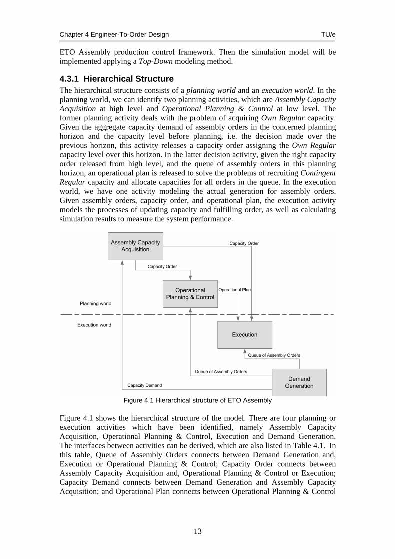
4.3.1 Hierarchical Structure The hierarchical structure consists of a planning world and an execution world. In the planning world, we can identify two planning activities, which are Assembly Capacity Acquisition at high level and Operational Planning & Control at low level. The former planning activity deals with the problem of acquiring Own Regular capacity. Given the aggregate capacity demand of assembly orders in the concerned planning horizon and the capacity level before planning, i.e. the decision made over the previous horizon, this activity releases a capacity order assigning the Own Regular capacity level over this horizon. In the latter decision activity, given the right capacity order released from high level, and the queue of assembly orders in this planning horizon, an operational plan is released to solve the problems of recruiting Contingent Regular capacity and allocate capacities for all orders in the queue. In the execution world, we have one activity modeling the actual generation for assembly orders. Given assembly orders, capacity order, and operational plan, the execution activity models the processes of updating capacity and fulfilling order, as well as calculating simulation results to measure the system performance.

Figure 4.1 Hierarchical structure of ETO Assembly

Figure 4.1 shows the hierarchical structure of the model. There are four planning or execution activities which have been identified, namely Assembly Capacity Acquisition, Operational Planning & Control, Execution and Demand Generation. The interfaces between activities can be derived, which are also listed in Table 4.1. In this table, Queue of Assembly Orders connects between Demand Generation and, Execution or Operational Planning & Control; Capacity Order connects between Assembly Capacity Acquisition and, Operational Planning & Control or Execution; Capacity Demand connects between Demand Generation and Assembly Capacity Acquisition; and Operational Plan connects between Operational Planning & Control


14

and Execution. We noticed here that more than one activity can share one interface as input, such as the interfaces of Queue of Assembly Orders or Capacity Order.

Interface Name Output of Activity Input for Activity Execution Queue of Assembly

Orders Demand Generation Operational Planning & Control

Capacity Demand Demand Generation Assembly Capacity Acquisition Execution

Capacity Order Assembly Capacity Acquisition Operational Planning & Control

Operational Plan Operational Planning & Control Execution Table 4.1 Interface between activities

Given the hierarchical structure, we will apply the Top-Down method to design and build the CPN simulation model. In section 4.3.2 we will first transform the hierarchical structure to the high level CPN architecture model. Then in section 4.3.3 we will extend the architecture model into detailed CP-nets.

4.3.2 CPN Architecture Model The hierarchical structure described in the previous section is transform to the CP-net as the high level architecture design shown in Figure 4.2. We have three steps to do that. 1) The planning and execution activities identified in the hierarchical structure are

mapped to transitions in CPN. Therefore we have transitions of “acquire capacity”, “plan & control”, “execute assembly”, “report” and “generate demands”, which are located in different hierarchical levels. We should notice that the Execution activity in Figure 4.1 is split into two transitions of “execute assembly” and “report”. This is for the clearance of different functionalities. “Execute assembly” updates capacity levels and changes order statuses. In sequence, “report” calculates average capacity cost and utilizations as the simulation result. Finally we add a single transition of “initialize” to set the initial environment parameters, because a simulation is meaningful only in a specified environment.

2) In the hierarchical structure, the interfaces between activities are mapped to places

in CPN. Therefore we have places of “capacity order”, “operational plan” and “demands” in Figure 4.2. We notice that “demands” is the only place definition for both interfaces of Capacity Demand and Queue of Assembly Orders. The reason behind is that these two interfaces have the same information source. Capacity Demand includes the aggregate information of orders. However Queue of Assembly Orders includes individual order-oriented information. We add an extra place of “statistics” to save the simulation result. Every place must be assigned with a color (data type) in CPN. The places with their colors are listed in Table 4.3. The definitions of basic colors are also listed in Table 4.2, which are combined into complex colors to represent system states in this model.

3) We connect transitions and places with arcs according to their relations in the

hierarchical structure.


15

Figure 4.2 Architecture of CPN model

Color Description color ID = int; The unique ID of each order color VOL = int; The volume of capacity by unit of person per week color D = int; Day color WK = int; Week color MON = int; The amount of money color PERCENT = int; Capacity utilization

Table 4.2 Basic Color definitions Place Color Description

capacity order

color CAP_ORDs = list CAP_ORD; color CAP_ORD = product D * VOL;

A list of capacity orders appointing Own Regular capacity level at certain time

operational plan

color OPR_PL = product D * VOL * ASS_PLs; color ASS_PLs = list ASS_PL; color ASS_PL = product ID * VOL * VOL * VOL * VOL;

At certain time, the required Contingent Regular capacity level and a list of assembly plans for considered orders. The assembly plan includes order ID, assignment for three kinds of capacity, and the work apart from finish

demands color ORDs = list ORD; color ORD = product ID * VOL * VOL * D * D;

A list of assembly orders including information of demand for Specialist and Regular capacities, start time and lead time for assembly

statistic color STAT = product WK*MON*PERCENT*PERCENT;

Simulation result including average cost and utilizations for Specialist and Own Regular capacities

Table 4.3 Places in the architecture model Up to now, the system is presented as a structure model including a number of transitions in hierarchy. Because hierarchical CP-nets are supported by CPN Tools, every transition represents a module or sub-process in this structure. We will elaborate every transition in the next section.


16

4.3.3 Detailed Model Design The detailed CP-nets of all modules in the architecture model will be depicted in this section. The design is based on the some assumptions which are included in Appendix B. Before elaborating each module separately, we first make clear its time attributes. Each activity occurs periodically, and its occurrence time and frequency has to be determined. In this model, we have a basic execution period, e.g. one week. So “execute assembly” and “report” occurs once a period. We assume that they occur at the end of a period, because their inputs cover all the orders which should be assembled in this period. We assume that those two planning modules occur at the beginning of a period. “Acquire capacity” works at the top level and its planning horizon is much longer than “plan & control” which works at the bottom level; i.e. the decision from the former is released less frequently than that from the latter. We also take into account the concept of Effectuation Lead Time, which is the time that passes between the moment a decision is made and the moment that the consequences of this decision can be observed [1]. The effectuation lead time for “acquire capacity” is longer than that for “plan & control”, because the lead times for acquiring Own Regular and Contingent Regular capacity are different. The four planning and execution modules discussed above have fixed occurrence frequencies. Therefore they follow a mechanism of fixed-increment time advance [14]. The occurrence of “generate demands” is not fixed, because the intervals between order arrivals are assumed to follow Exponential distribution. The occurrence of the current order generation will determine the time interval till the next order arrival. Therefore the module of “generate demands” follows a mechanism of next-event time advance [14]. We should notice that there is a lead time between the moment an order is generated and the moment its assembly starts. Table 4.4 lists the time attributes of all planning and execution activities. Due to the different time attribute, each activity will be designed as independently running sub-process.

Module Name Occurrence Time Frequency Effectuation LT acquire capacity Beginning of a week Once every four weeks Four weeks plan & control Beginning of a week Once a week One week

execute assembly End of a week Once a week NA report End of a week Once a week NA

generate demands By previous occurrence Possion distributed NA Table 4.4 Time attributes of modules

In the following part, we will show the detailed sub-process design inside each module, including “initialize”, “generate demands”, “execute assembly”, “report” and “acquire capacity”. For the detailed design of “plan & control”, please refer to the Master thesis from Wu [24]. Initialize This module initializes the simulation environment, which includes the start times of the other sub-processes, initial capacity levels and capacity unit costs. Figure 4.3 shows the sub-process of “initialize”.


17

Figure 4.3 Sub-process of “initialize” There is only one transition – “initialize”, to set up the environment. The place “start” fires this transition at the very beginning of the simulation. After its execution, the places of “start_GD”, “start_AC”, “start_PC”, “start_EA” and “start_R” will hold the start times of all the other sub-processes of “generate demands”, “acquire capacity”, “plan & control”, “execute assembly” and “report”. These start times are appointed by giving time values behind “e@+” on output arcs, and these values are determined by the time attributes of those modules. The transition “initialize” also gives the initial level and unit cost of all capacities as “cap_init” and “uc_init”, both of which are pre-defined constants. The places mentioned above are all tagged with different Fusions (Fusion 1…Fusion 7). After “initialize” is fired, the places in other sub-processes with corresponding Fusion tags will also receive certain values. This behaviour results from the communications which are built between this module and other modules. Generate demands This module generates the actual assembly orders. Figure 4.4 shows the sub-process of “generate demands”.

Figure 4.4 Sub-process of “generate demands” In this sub-process, the transition of “start” initializes the place of “ID” which is the input for generating an assembly order. After that, the transition of “generate


18

demands” generates the actual assembly orders repetitively, which are stored at the place of “demands”; and it also manages the ID and arrival time of the next assembly order. The outcome of this sub-process is to renew the queue of assembly orders. The function of “ord_gen()” generates an order with capacity demands for Specialist and Regular capacities as well as the start time and lead time of assembly. The function of “interarrivaltime()” decides the time interval till the generation of the next order. Execute assembly At the end of every period, this module simulates updating the capacity levels, fulfilling assembly orders by changing among different statuses of Not-Ready, Waiting and Work-In-Process, and recording the usages of all capacities in this turn. Figure 4.5 shows the sub-process of “execute assembly”.

Figure 4.5 Sub-process of “execute assembly”

There are three transitions and nine places in this sub-process. The places of “start”, “s1” and “s2” indicate that these three transitions are executed in sequence. Other places are either input, output places or both. Table 4.5 lists these places and their color definitions, except for “capacity order”, “operational plan”, and “Not-Ready” because they have been introduced in the architecture model. We notice that “Not-Ready” is the place mapped from “Demands” in the architecture model, because every order is by default with the status of Not-Ready after its generation. In the 1st step, given the inputs from “capacity order”, “operational plan” and “capacity”, the transition of “update capacity” renews the levels of Own Regular and Contingent Regular capacities, and also records the changes of them. The guard on “update capacity” takes the correct operational plan which should be executed in the


19

considered period. One modeling problem here is that, the module of “acquire capacity” releases decision to the place of “capacity order” once every four periods (Table 4.4), i.e. the planning horizon is four periods, and the cycle of execution is one period. Therefore in an execution period, there is not always an available token held by “capacity order”. Only in the first period of a cycle of four periods, “update capacity” is supposed to renew the Own Regular capacity level, and it should do nothing in the rest of time. The capacity order here is defined to have an element of time stamp indicating when this capacity order is available. The time stamp is specified by the module of “acquire capacity” when it releases a capacity order. So in every execution period “update capacity” evaluates the available time of each capacity order; if there is one matching the current system time, “update capacity” expects a new capacity order to be executed; if there is nothing, it doesn’t update the Own Regular capacity level in this period. In the 2nd step, the transition of “NR-W” delivers the orders from “Not-Ready” to “Waiting” if their start times meet the execution time. Thus this transition updates the token lists at both “Not-Ready” and “Waiting” by evaluating the token from “Not-Ready”. In the 3rd step, the transition of “W-WIP” transfers the orders between “Waiting” and “WIP” depending on the content of concerned operational plan. Just like “update capacity”, the guard on “W-WIP” also takes the correct operational plan, which includes the orders under consideration in this period. Four functions should be explained here: “wip_up(wip,opl)” returns the orders with WIP which still appear in the operational plan; “wip_for(wt,opl)” returns the orders with Waiting which appear in the operational plan; “wip_wt(wip,opl)” returns the orders with WIP which don’t appear in the operational plan any more; “w_bak(wt,opl)” returns the orders with Waiting which don’t appear in the operational plan yet. This transition also records the usages of all three kinds of capacity in this period by aggregating the capacity assignment information in the operational plan. Place Color Description capacity color CAP = product SPE_C *

OWN_C * CON_C; color SPE_C = product VOL * VOL; color OWN_C = product VOL * VOL * VOL; color CON_C = product VOL * VOL * VOL;

A product data type has levels of three kinds of capacity. In SPE_C, the 1st VOL is the capacity level, and the second is surplus capacity in the considered period. In OWN_C and CON_C, the 1st VOL is the capacity level, the 2nd is the surplus capacity, and the 3rd is the capacity change in the considered period.

Waiting color WTs = list WT; color WT = product ID*VOL*VOL*D;

A list of orders with the status of Waiting. WT defines the order ID, workload for both Specialist and Regular capacities, and the due date of this order.

WIP color WIPs = list WT; color WIP = product ID * VOL * VOL * VOL * VOL * D;

A list of orders with the status of Work-In-Process. WIP defines the order ID, the capacity usages for all three kinds, workload left after this period, and the due date of this order.

Table 4.5 Some places in the “execute assembly” Report Following the “execute” in each period, this module works in sequence to calculate the capacity cost and the utilizations of Specialist and Own Regular capacities in this


20

period. Finally it calculates the statistical data of average cost and utilizations as the result of the simulation model. Figure 4.6 shows the sub-process of “report”. There are three transitions and eleven places in this sub-process. The places of “start”, “s1” and “s2” indicate that these three transitions are executed in sequence. The place of “unit cost” stores a set of system parameters about all unit costs. The places of “cost” and “utilization” are intermediaries holding the execution results in this period. The place of “counter” maintains the number of execution periods, and then the values from them are used to calculate statistical data. The place of “statistic” is input/output place for present simulation result. Table 4.6 lists all places of and their color definitions, except for what has been introduced before.

Figure 4.6 Process of “report”

Place Color Description unit cost color COS = product MON * MON *

MON * MON * MON; The Product data represents five kinds of unit costs, which from left to right are maintaining specialist, maintaining own regular, changing own regular, maintaining contingent regular and changing contingent regular.

cost color COS_T = product WK * MON; It holds the capacity cost in a certain period.

utilization color UTIL = product WK * PERCENT * PERCENT;

It holds two capacity utilizations in a certain period.

statistic color STAT = product WK * MON * PERCENT * PERCENT;

It presents the system result, including the number of execution periods, average cost and two average utilizations

Completion color HISs = list HIS; color HIS = product ID * D;

A list of orders with the status of Completion. HIS defines the order ID and the completion date.

Table 4.6 Some places in the “report”


21

In the 1st step, given the unit costs, the transition of “calcu_cost” calculates the total capacity cost in this period. It also takes the input from “capacity” and reset all parts which record the capacity changes back to zero. In the 2nd step, according to the surplus capacities, the transition of “calcu_utilization” calculates the utilizations of Specialist and Own Regular capacities in this period. It also takes the input from “capacity” and reset all parts which record the surplus capacities back to zero. In the 3rd step, the transition of “complete” takes the values from “cost” and “utilization” and then calculates the statistical results. The code segment inscription on “complete” performs the calculation of average cost, average specialist utilization, and average own-regular utilization. This transition also delivers the orders from “WIP” to “Completion” if their workloads left are zero after this period of execution. Thus this transition updates the token lists at both “WIP” and “Completion” by evaluating the token from “WIP”. Acquire capacity This sub-process has two inputs – “demands” and “capacity order”, and one output – “capacity order”. It releases the decision on Own Regular capacity level, which will make effect after 4 weeks from the planning time. Figure 4.7 shows the sub-process of “acquire capacity”.

Figure 4.7 Sub-process of “acquire capacity” The transition “scope” takes a list of assembly orders which should be considered for planning in this horizon and saves them at “dem_in”. Then the transition “acquire capacity” aggregates the demand for Regular capacity, calculates the Own Regular capacity level at the time of planning, and then generates a capacity order to assign a new level of Own Regular capacity for the considered the planning horizon. We notice that the capacity level at the planning time is achieved from the previous capacity order instead of “capacity” which presents the system state of all capacities.


22

This is because of the effectuation lead time of this planning activity. At this point the capacity level is still not effectuated by the previous capacity order.

4.4 Test of Validity In this section, we run this simulation model in different environment settings for certain number of periods. Thus we find proper ways to validate our model.

4.4.1 Simulation Two things have to be done in order to start simulation: setting environment parameters and defining the number of execution periods. Parameters setting A set of parameters are used to differentiate the behaviors of this CPN simulation. Figure 4.8 shows an example of setting parameters, which are represented as constants in CPN.

Figure 4.8 Environment parameters setting

Operation In this simulation, we consider a business cycle of 6 years (suggestion in [15]). The unit of execution period is 1 week. Therefore a whole business cycle consists of T periods, T=312 (52 weeks per year). So in the test, we define each sample of simulation consisting of 312 execution periods. The statistical data is presented at the place “statistic” with the color of “STAT”. An example of result looks like: (312, 198, 85, 87). In this simulation model, the statistical data stops changing after the model executes for 312 periods. In this way we can see the simulation result of a business cycle in each test sample. The simulation tool in CPN Tools is used to execute the CPN model. We select “FastForward” option to directly see the simulation result. In order to make the


23

model run 312 periods, we change the “Number of steps” attribute of “FastForward” to “5000” (Figure 4.9). This number is large enough to ensure that the simulation runs for at lease 312 periods. For detailed operation of the simulation tool, please refer to Appendix F.

Figure 4.9 Number of steps

4.4.2 Validation Validation is the process of determining whether a simulation model is an accurate representation of the system, for the particular objectives of the study [Fishman and Kiviat (1968)]. In [14] Validation is also discussed from several perspectives. Our objective is not to validate the individual planning modules with decision making processes and functions, but the hierarchical structure as a whole integrating and coordinating decision functions, as well as simulating their executions. We believe the hierarchical structure design can be validated through testing the generic qualitative behaviours and analyzing the coordination between decision functions. Therefore we have two focuses: 1) we will first formulate some hypotheses and then see whether the decision structure, as a whole, performs the supposed behaviours; 2) we will analyze the interaction and coordination between decision functions in this structure, from the qualitative behaviours according to different environment settings. The following part consists of a series of tests. Test 1 We start from the basic and obvious behaviour of this model. This model has an activity to generate assembly demands. The arrival time and demand of an order follow some kinds of distribution. In this test, we will change the parameters of those distributions in order to change the attributes of order generation. Therefore we can see the relative outcomes. First we let some parameters to be fixed as shown in Table 4.7. Here we must notice that the setting of unit costs (parameter of uc_init). According to [15], normally maintaining Specialist capacity is the most expensive. And for regular job, maintaining Contingent Regular capacity is more expensive than maintaining Own


24

Regular capacity. But changing Contingent Regular capacity is cheaper than changing Own Regular capacity. That is the reason behind deciding uc_init.

Para. Name ec_lt ass_lt cap_co cap_init uc_init spe_on Value 8 4 3 ((6,6),(20,20,0),(0,0,0)) (10,4,3,8,1) 1

Table 4.7 Stable parameters setting Then we do five groups of tests (Table 4.8) by changing the value of parameters interarrival, ED and SD. The first group is default setting. In the second group, we change the interarrival to 14.0, and keep ED and SD constant. And in the third group, we change the interarrival to 5.0. These two groups indicate that the frequency of order coming is either decreased or increased. In the forth group we change the ED from 20.0 to 30.0, and keep SD and interarrival constant. And in the fifth group we change the ED from 20.0 to 15.0, and keep SD and interarrival constant. These settings indicate that the demand for each order is either increased or decreased. After executing each group for 10 times, we get the results shown in Table 4.9 as well as the 90%-confidence intervals, according to the formula for a t-distribution [14].

Group No. interarrival ED SD 1 7.0 20.0 4.0 2 14.0 20.0 4.0 3 5.0 20.0 4.0 4 7.0 30.0 4.0 5 7.0 15.0 4.0

Table 4.8 Test for 5 groups of parameters Gr. No. 1 2 3 4 5 6 7 8 9 10 C.I.

a.c. 136 151 146 139 135 149 148 151 141 143 143.9±3.5 a.u.s 72 79 71 74 75 73 73 70 73 74 73.4±1.4

1

a.u.o 83 87 83 87 84 83 83 81 83 82 83.6±1.3 a.c. 100 104 107 108 102 102 103 109 108 107 105.0±1.8

a.u.s 58 59 61 61 58 56 62 60 55 63 59.3±1.5 2

a.u.o 67 71 69 71 66 66 70 68 63 74 68.5±1.9 a.c. 171 181 172 176 179 177 174 163 181 190 176.4±4.2

a.u.s 81 80 77 83 79 79 82 76 78 81 79.6±1.3 3

a.u.o 89 88 88 91 88 90 90 87 88 91 89.0±0.8 a.c. 188 196 189 204 193 203 187 200 194 201 195.5±3.7

a.u.s 85 85 83 86 83 89 82 86 90 84 85.3±1.5 4

a.u.o 89 89 88 89 86 90 87 88 92 88 88.6±1.0 a.c. 118 125 123 117 124 126 120 119 123 119 121.4±1.9

a.u.s 64 70 70 64 65 65 66 67 65 63 65.9±1.4 5

a.u.o 78 81 82 77 78 80 79 80 79 78 79.2±0.9 a.c: Average Cost a.u.s: Average Utilization of Specialist a.u.o: Average Utilization of Own Regular

Table 4.9 Result of Test 1 In this test, we adjust the attributes of order generation activity. We can hypothesize intuitively that the average cost and utilizations will increase if either the volume of demand or the frequency of order arrival is increased, and vice versa. From the test, we see that the model reflects this behaviour. Figure 4.10 shows the comparison for 5 groups of data. On one hand, in group 2 and 3, the frequency of order arrival is altered. As a result, the cost and utilizations in group 1 is bigger than those in group 2 and smaller than those in group 3. On the other hand, in group 4 and 5, the volume of


25

demand is altered. And the result shows, the cost and utilizations in group 1 are smaller than those in group 4 and bigger than those in group 5. Therefore the model behaves the same with our hypothesis.

100

120

140

160

180

200

1 2 3 4 5

Ave

rage

Cos

t

50

60

70

80

90

100

1 2 3 4 5

Avg

. Util

. of S

epci

alis

t

50

60

70

80

90

100

1 2 3 4 5

Avg

. Util

. of O

wn

Reg

ular

Figure 4.10 Comparison for different order attributes

Test 2 In the design of Operational Planning & Control activity, we assume that after doing specialist job, the remaining Specialist capacity might be used for regular jobs. (Refer to Master thesis from Wu [24]) And in this model, we have a parameter spe_on acting as the switch to open or close this behaviour. So in this test, we will see the difference between on and off of spe_on. The setting of other stable parameters is shown in Table 4.10. And we have two groups of test for switching spe_on shown in Table 4.11.

Para. Name ec_lt ass_lt cap_co cap_init Value 8 4 3 ((6,6),(20,20,0),(0,0,0)) Para. Name interarrival ED SD uc_init Value 7.0 20.0 4.0 (10,4,3,8,1)

Group No. spe_on 1 1 2 0

Table 4.10 Stable parameters Table 4.11 Test for 2 groups

Gr. No. 1 2 3 4 5 6 7 8 9 10 C.I.

a.c. 138 142 143 140 138 147 149 152 142 142 143.3±2.7 a.u.s 74 77 75 71 74 74 75 77 71 72 74.0±1.3

1

a.u.o 83 85 84 81 85 84 85 86 82 82 83.7±1.0 a.c. 149 167 154 161 159 159 154 160 151 156 157.0±3.1

a.u.s 23 28 24 26 26 26 24 26 24 25 25.2±0.9 2

a.u.o 95 93 95 92 92 92 91 91 92 95 92.8±0.9 a.c: Average Cost a.u.s: Average Utilization of Specialist a.u.o: Average Utilization of Own Regular

Table 4.12 Result of Test 2 If the extra Specialist capacity is not used, the available resources for regular jobs are smaller, because we let it be always sufficient and there must be surplus. In this case, obviously the Specialist utilization will be decreasing, and the Own Regular utilization will be increasing because much more workload will be sustained by it. Furthermore, without the resource from surplus Specialist capacity, there is more chance that an order is not finished until the “last minute”. So there is more chance to recruit Contingent Regular capacity in order to fulfill an order on time, because the


26

mechanism behind recruiting Contingent Regular capacity is that it will be recruited only if it is really necessary, i.e. without Contingent capacity, the order will not be finished on time. So in this case, the cost will be increasing because there will be extra cost for Contingent capacity. In this test, we make a hypothesis that after switch the spe_on from on to off, the cost and the own-regular utilization will increase, and the specialist utilization will decrease. Table 4.12 shows the results of 10 samples for each group as well as the 90%-confidence intervals, which accord with our hypothesis. Test 3 In the design of Capacity Acquisition activity, given the capacity demand and the current capacity level, we use a simple function to decide the Own Regular capacity level for the next horizon. In this function, a decision coefficient∆ is used, which is represented as a parameter cap_co in the model. We will see the influence of this parameter on the simulation results. This test consists of two sections, with another parameter of spe_on being on and off. Finally we will analyze their results. Section 1 The setting of other parameters is shown in Table 4.13. And we have five groups of test with different value of cap_co. And in the first section, we let spe_on open (Table 4.14). In these five groups, cap_co is set to be decreasing from 10 until it reaches 0 in the fifth group. If cap_co is set to 0, the Own Regular capacity is maintained constant, i.e. we disregard the effect of the planning activity of Capacity Acquisition. So the result can more or less prove the effect of a decision function in a hierarchical decision structure, even though the algorithm we selected for Capacity Acquisition might not be much effective. When we look at this algorithm (Appendix B), we can see the selection of decision coefficient∆ determines the flexibility of the decision on acquiring capacity. Given 0>∆ , the bigger∆ is, the less frequently the Own Regular capacity fluctuates. But if it fluctuates, the extent of its fluctuation is bigger. On the contrary, the smaller∆ is, the more frequently the Own Regular capacity fluctuates, but the extent of its fluctuation is small.

Para. Name ec_lt ass_lt cap_init Value 8 4 ((6,6),(20,20,0),(0,0,0)) Para. Name interarrival ED SD uc_init Value 7.0 20.0 4.0 (10,4,3,8,1)

Table 4.13 Stable parameters setting

Group No. spe_on cap_co 1 1 10 2 1 7 3 1 4 4 1 1 5 1 0

Table 4.14 Test for 4 groups of parameters in Section 1 We believe the planning activity of Capacity Acquisition makes some sense in the hierarchical decision structure. Thus we suppose that if we ignore its effect in planning (cap_co = 0), the outcome will be the worst. However we don’t know yet how the flexibility of acquiring capacity affects the results. Thus we expect a conclusion on the best choice for cap_co from the simulation. Table 4.15 lists the results of 20 samples for each group as well as the 90%-confidence intervals; and in Figure 4.11, we compare the results of average cost and average utilization of Own Regular for those five groups.


27

1 2 3 4 5 Gr. No. a.c. a.u.s a.u.o a.c. a.u.s a.u.o a.c. a.u.s a.u.o a.c. a.u.s a.u.o a.c. a.u.s a.u.o 1 146 72 82 145 75 85 143 70 82 148 72 80 148 71 83 2 145 72 83 141 70 84 142 76 87 153 75 84 149 65 79 3 138 74 84 133 73 83 151 74 83 140 76 84 147 75 86 4 143 67 81 142 76 87 141 77 86 139 76 84 149 63 78 5 149 70 82 145 71 83 144 78 86 148 73 82 149 72 84 6 147 78 88 146 73 85 148 72 84 138 76 84 151 71 81 7 155 76 85 146 68 80 143 73 83 144 76 84 146 66 80 8 146 67 80 140 77 85 146 74 84 144 72 82 159 72 82 9 140 73 83 135 69 80 148 71 82 143 71 85 151 74 85

10 138 70 82 139 74 83 143 74 85 146 74 82 150 73 84 11 145 72 83 141 70 85 153 72 82 148 73 82 151 71 81 12 138 74 84 143 75 86 145 73 83 144 76 84 146 66 80 13 143 67 81 146 73 84 150 73 86 144 72 82 159 72 82 14 149 70 82 143 78 87 142 74 83 143 72 85 150 65 79 15 147 78 88 136 77 87 151 68 81 146 74 82 151 74 82 16 155 76 85 138 75 84 149 72 82 143 75 85 150 73 82 17 146 67 81 141 67 79 143 75 85 147 70 81 146 66 79 18 140 73 84 145 69 84 144 75 84 149 73 84 154 71 80 19 138 70 82 137 70 81 150 77 87 144 70 82 157 70 82 20 150 77 85 139 76 87 139 74 85 149 71 84 154 73 83

C.I. 144.9 ±1.9

72.2 ±1.3

83.3±0.8

141.0 ±1.4

72.8 ±1.2

84.0±0.9

145.8±1.5

73.6±0.9

84.0±0.7

145.0±1.3

73.4±0.8

83.1 ±0.5

150.9 ±1.5

70.2±1.3

81.6±0.8

a.c: Average Cost a.u.s: Average Utilization of Specialist a.u.o: Average Utilization of Own Regular

Table 4.15 Result of Test 3 Section 1

135

140

145

150

155

1 2 3 4 5

Ave

rage

Cos

t

80

81

82

83

84

85

1 2 3 4 5

Avg

. Util

. of O

wn

Reg

ular

Figure 4.11 Comparison for different coefficients with using Specialist

When we look at the results of average utilization of Specialist, they are not comparable because all their confidence intervals are overlapped. When we look at average utilization of Own Regular, the result of group 5 is lower than those from other four groups. However in those four groups, their results are not comparable, because their confidence intervals are overlapped. When we look at average cost, the results of groups 1, 3 and 4 are not comparable. However the result of group 2 (cap_co = 7) is the lowest and the result of group 5 (cap_co = 0) is the highest.


28

Section 2 In this section, we will switch spe_on off, and then test another five groups (Table 4.16) with the same settings of cap_co as in the first section. When decision in Operational Planning & Control is made, the permission to use surplus Specialist capacity might weaken the relationship between the level of Own Regular capacity and recruiting Contingent Regular capacity, because the part of surplus Specialist capacity might act as a buffer. So turning down spe_on might reflect more about the interaction between two decision functions. In this section, it makes no sense to analyze the specialist utilization. We still suppose that if we set cap_co as 0, the outcome is the worst, and we don’t know which one is the best. Table 4.17 lists the results of 20 samples for each group as well as the 90%-confidence intervals. In Figure 4.12, we compare the results of average cost and average utilization of Own Regular for those five groups.

Group No. spe_on cap_co 1 0 10 2 0 7 3 0 4 4 0 1 5 0 0

Table 4.16 Test for 4 groups of parameters in Section 2

1 2 3 4 5 Gr. No. a.c. a.u.s a.u.o a.c. a.u.s a.u.o a.c. a.u.s a.u.o a.c. a.u.s a.u.o a.c. a.u.s a.u.o 1 164 28 94 153 24 93 161 26 91 159 25 93 176 24 85 2 152 24 94 159 25 94 162 26 93 165 26 90 164 26 88 3 158 26 93 156 25 91 169 29 92 169 26 90 168 26 89 4 159 26 93 154 23 91 154 25 90 165 25 90 159 24 86 5 156 26 90 154 24 94 155 24 91 163 25 88 166 26 90 6 150 24 92 159 26 95 149 23 95 153 23 90 171 26 87 7 162 26 90 153 24 96 167 28 93 167 26 89 161 25 89 8 152 24 92 159 26 92 154 24 95 158 24 88 160 25 84 9 155 26 96 151 24 94 161 26 92 159 24 94 170 28 90

10 153 25 91 144 23 91 159 26 92 175 27 86 166 25 84 11 164 28 94 146 22 91 158 26 93 165 27 90 182 28 89 12 157 23 93 158 26 95 163 27 92 156 24 90 164 27 92 13 162 27 93 152 24 90 157 25 92 161 25 88 169 26 88 14 160 25 93 154 25 92 160 25 91 164 24 88 161 25 85 15 162 27 89 153 23 90 166 26 90 164 27 92 158 24 86 16 163 24 89 148 23 90 159 26 93 164 24 87 167 26 89 17 156 24 89 154 26 95 158 26 93 154 23 92 163 26 90 18 163 23 92 155 24 90 168 26 92 174 28 92 158 24 97 19 155 25 95 160 27 94 159 26 95 170 28 91 166 24 79 20 156 26 91 157 24 90 162 27 93 163 26 93 166 27 93

C.I. 158.0 ±1.6

25.4 ±0.6

92.2±0.7

154.0 ±1.6

24.4 ±0.5

92.4±0.8

160.1±1.9

25.9±0.5

92.4±0.5

163.4±2.2

25.4±0.6

90.0 ±0.8

165.8 ±2.2

25.6±0.5

88.0±1.4

a.c: Average Cost a.u.s: Average Utilization of Specialist a.u.o: Average Utilization of Own Regular

Table 4.17 Result of Test 3 Section 2


29

150

155

160

165

170

1 2 3 4 5

Ave

rage

Cos

t

86

87

88

89

90

91

92

93

94

1 2 3 4 5

Avg

. Util

. of O

wn

Reg

ular

Figure 4.12 Comparison for different coefficients without using Specialist

When we look at average utilization of Own Regular, the result of group 5 (cap_co = 0) is lower than those from the first three groups but a little bit overlapped with that of group 4. As for average cost, it is the same situation. The result of group 5 is higher than those of groups 1, 2 and 3 but overlapped with group 4. Group 2 (cap_co = 7) has the lowest average cost. Analysis of Section 1 and Section 2 We summarize the results from Section 1 and Section 2 in order to see whether our hypothesis is true and concludes which is the best choice for cap_co. We list all the facts about cap_co from this test in Table 4.18.

Average Cost Average Utilization of Own Regular Section 1

(spe_on = 1) 7 – lowest cost 0 – highest cost

0 – lowest utilization

Section 2 (spe_on = 0)

7 – lowest cost 0 – higher than 10, 7, 4

0 – lower than 10, 7, 4

Table 4.18 Facts about the choice for cap_co from the test In Section 1, we see that the choice of 0 performs the worst. In Section 2, we see that the choice of 0 performs worse than most other choices. Thus this coincides with our hypothesis on ignoring the planning activity of Capacity Acquisition. So its effect is proved in the hierarchical decision structure. In both sections, from the perspective of average cost, we see that the choice of 7 always has the lowest cost. So we conclude that the best choice for cap_co is 7.

4.5 Summary In this chapter we show the development of a generic simulation model in the context of ETO Assembly. In the process, the concept of hierarchical decision structure has been successfully translated into high level CPN architecture. And the planning and execution sub-processes have been implemented inside the structure. After implementation, we have validated the qualitative behaviours of this model by simulations in different environment settings. In this model, the hierarchical decision


30

structure works over the relation between aggregate capacity acquisition in long horizon and allocation in short horizon. So in general, we have modeled the aggregate-allocate decision making in the context of Long-Term decision vs. Short-Term decision. In the process of development, the Top-Down method is practiced, from the architecture model to sub-process models.

Chapter 5 Conclusion TU/e

31

5 Conclusion In this project, we have presented a CPN simulation model for modeling a single stage of engineer-to-order production system. The model only focuses on one SCOP problem of capacity planning. The hierarchical decision structure is the core of the model, which serves as an overview of all planning activities as well as their relations. The architecture model as a framework provides a generic environment for a specific production system. The environment enables the planning modules in hierarchy to interact with each other. The result of coordination can be tested through execution activities. For the research on production control problems, different decision functions used by planning activities can be modeled in CPN based on the given framework and then separately integrated within the same environment, i.e. the same other planning activities at different hierarchical levels and the same execution activities. Thus the performance of those decision functions can be tested and compared. Our experience shows that the environment (hierarchical structure) is presentable, even for audiences not familiar with CPN. In general, a generic architecture model plus specific functional modules consist of the Top-Down simulation model. CPN goes beyond the capability of a programming language. Instead it is a graphical modeling language for real-life processes while also having some competences from programming language. A CPN model can be easily applied to present real-life system processes and define system states. Furthermore a CPN model is executable so that the system states can be changed according to certain algorithms. A simulation can be also realized in regular programming language, e.g. Object-Oriented programming language. The planning and execution activities can be designed as different classes with states, e.g. JAVA Bean. Then another class can be designed taking the idea of hierarchical structure. However, this kind of simulation just takes a set of inputs and then presents the simulation result. Thanks to the primitives from Petri Nets, a CPN simulation model makes a user easily understand how the result is achieved because a visible model of the system is also presented. This is useful for research on decision functions. However one disadvantage of a CPN model is that the execution speed is clearly slower than a regular computer program, e.g. Delphi program, even though a user can select “FastForward” (Appendix F) to see the result directly. (When we conducted the case design for a known Delphi program, with the same environment setting, the execution time of Delphi program was about 3 seconds, whereas that of the CPN imitated model was nearly 30 seconds) CPN Tools has powerful functions for developing and executing CPN models. Its capability to support multiple and hierarchical CP-nets facilitates the Top-Down modeling method. The definitions of Port/Socket and Fusion enable the synchronized communications among places in hierarchical and different CP-nets. However it is only possible to assign a place with Fusion if the place is neither a Socket nor a Port. This means that if we use a set of Fusion places to represent one system state and it includes places connecting super/sub pages, we must break their Port/Socket relations. This debases the readability of a set of hierarchical CP-nets from the perspective of input/output. Anyhow, the capability for defining hierarchical CP-nets is the key property of CPN Tools which makes it suitable for designing the SCOP problem as a hierarchical structure. We notice that there are simulation packages in the market,

Chapter 5 Conclusion TU/e

32

which can build the simulation in the same context, e.g. Arena. We didn’t use a simulation package in this project, and here we just give simple discussion on it. [14] In Arena a user can construct a high level process including several modules with different functions. Arena provides built-in features for all general-purpose modules. Thus a user just has to modify some attributes in the dialog box related to a module in order to make specific design. This coincides with our modeling method with CPN Tools. Compared to CPN Tools, Arena has two advantages: 1) minimal programming work; and 2) graphical presentation and animation in good quality. However CPN Tools provides more flexibility for modeling any situations, and it is free to use with a license. For the graphical presentation and animation, CPN Tools enables a model to have interfaces for external programs, so that they can be done outside. (See Logistic Games in CPN Tools [18]) This project served as a trial of design research with CPN Tools; it showed how to apply a new information technology in a specific background area. The concept of planning in hierarchy was reflected in our CPN simulation model. In the design process, we have shown that CPN Tools is suitable to model SCOP problems as a hierarchical decision structure, not only from the perspective of technology capabilities, but also from the perspective of project engineering. In this project, we have experienced a complete design process from understanding background knowledge and concept, to designing, to implementing and to testing finally. The CPN simulation model of ETO consists of 8 pages, 73 places, 26 transitions, 38 color definitions, and 59 functions. Two trainees with some CPN experience in this project spent 3 months finishing the ETO case design. The time is reasonable for using a simulation to prove a concept. We have made a number of assumptions for planning and execution activities in the specific ETO situation. Some assumptions are simple and not realistic but help us build the model and answer the research question, because our goal is the suitability of CPN for SCOP design by a complete model instead of the research on SCOP. In the future, however, this production situation can be described more complex, more SCOP problems can be formulated, and more decision functions can be leveraged in the design with CPN Tools.

Reference TU/e

33

Reference 1. De Kok, A.G. and Fransoo, J.C. Chapter 12: Planning Supply Chain Operations:

Definition and Comparison of Planning Concepts. In Handbooks of Operations Research: Supply Chain Management: Design, Coordination and Operation. Eindhoven University of Technology, 2003.

2. Bertrand, J.W.M. and Muntslag, D.R. Production Control in Engineer-To-Order Firms. In International Journal of Production Economics, 30-31 (1993) 3-22, Elsevier, Amsterdam, 1993

3. Bertrand, J.W.M., Wortmann, J.C. and Wijngaard, J. Production Control, A Structural and Design Oriented Approach, Elsevier, Amsterdam, 1990

4. Meal, H.C. (1984). Putting production decisions where they belong. In Harvard Business Review, 84: 102-111, 1984

5. Jensen, K. A Brief Introduction to Coloured Petri Nets. University of Aarhus. 6. Van der Aalst, W.M.P. Chapter 6, 7 in Process Modelling, lecture notes,

Eindhoven University of Technology. 7. De Kok, A.G. Planning under non-stationary stochastic demand and finite

capacity, lecture note 1C240, Eindhoven University of Technology. 8. Jensen, K. An Introduction to the Practical Use of Coloured Petri Nets. University

of Aarhus, 1996 9. Kristensen, L.M., Christensen, S. and Jensen, K. The practitioner’s guide to

Coloured Petri Nets. Springer-Verlag, 1998 10. Comparison of integrated approach and aggregation-decomposition approach.

Delphi program. 11. CPN Group. http://www.daimi.au.dk/CPnets/ 12. Hevner, A.R., March, S.T., Park, J. and Ram, S. Design Science in Information

Systems Research. In MIS Quarterly, Vol. 28 No.1, 75-105, March 2004. 13. Hendry, L.C. and Kingsman, B.G. Production planning systems and their

applicability to make-to-order companies. In Europe Journal of Operational Research, 40 (1989) 1-15, Elsevier, Amsterdam, 1989

14. Law, A.M. and Kelton, W.D. Chapter 1, 3, 4, 5, 9 in Simulation Modeling and Analysis, 3rd edition. ISBN 0-07-116537-1, McGraw-Hill, 2000

15. Bertrand, J.W.M. and van Houtum, G.J.J.A.N. Decision function design. OPAC LCS design group, Eindhoven University of Technology, 2004

16. Bertrand, J.W.M. and van Houtum, G.J.J.A.N. A reference model for operations planning and control in multi-project companies. OPAC LCS design group, Eindhoven University of Technology, 2004

17. Petri Nets World. http://www.informatik.uni-hamburg.de/TGI/PetriNets/ 18. Logistic Games in CPN Tools. http://is.tm.tue.nl/staff/wvdaalst/LOGgames/ 19. Vanderfeesten, I., van der Aalst, W.M.P and Reijers, H. Modeling a product based

workflow system in CPN tools. Eindhoven University of Technology, 2005 20. Günther, C.W. and van der Aalst, W.M.P. Modeling the Case Handling Principles

with Colored Petri Nets. Eindhoven University of Technology, 2005 21. Pesic, M. and van der Aalst, W.M.P. Modeling Work Distribution Mechanisms

Using Colored Petri Nets. In Beta Working Paper Series, Eindhoven University of Technology, 2005

22. Netjes, M., van der Aalst, W.M.P. and Reijers, H. Analysis of resource-constrained processes with Colored Petri Nets. Eindhoven University of Technology, 2005

Reference TU/e

34

23. Jensen, K. Coloured Petri Nets. Basic Concepts, Analysis Methods and Practical Use. Springer-Verlag, 1992.

24. Wu, D. HPP Design with CPN Tools, Master Thesis. Eindhoven University of Technology, 2005

Appendix A. Test Case: Simulating a Known Model TU/e

35

Appendix A. Test Case: Simulating a Known Model Before designing the simulation model of engineer-to-order, we first use CPN Tools to model an existing case which includes a hierarchical decision structure. A simulation of this case has been implemented in Delphi already. Thus an imitation of the Delphi program has three advantages which let us 1) understand the concept of hierarchical decision structure; 2) apply the Top-Down modeling method; and 3) get acquaintance with CPN Tools.

A1. Introduction A case of “Planning under non-stationary stochastic demand and finite capacity” [7] is selected. The case deals with production order release according to demand and production capacity in specified situations. In this lecture note, the author lists and discusses two approaches to solve the planning problem. One approach is to provide integrated decision for production planning; while another one is to release production decisions hierarchically, which includes an aggregation-decomposition decision making process. The case is used for proving that aggregation-decomposition approach is better than integrated approach. Therefore a hierarchical decision making mechanism has its positive sense. The conclusion is drawn through formulating two approaches into models and realizing them in a simulation with Delphi [10].

Figure A1 Delphi simulation program

The Delphi program has the functionalities such as defining problem size, inputting environment parameters and simulating the planning process. In the result page, the “P2 service level”, “Inventory capital”, “Total cost” and “Average cost” have been presented to measure the performance of two planning approaches. The results are deterministic and prove that the aggregation-decomposition approach is superior.


36

However there are two problems with this Delphi simulation: 1) a user can not see the detailed decision making process from the simulation; 2) the simulation of aggregation-decomposition approach doesn’t reflect a hierarchical decision structure, even though it takes the idea of making decision in hierarchy. The aggregation-decomposition approach in this case can serve as a good example for modeling using CPN Tools. We will imitate the aggregation-decomposition planning approach and present the average production cost as the simulation result. The result data from Delphi program can be regarded as a benchmark to evaluate our CPN model.

A2. System Description In this case, we consider the planning of a product family consisting of N items under non-stationary stochastic demand and finite capacity under a rolling schedule regime [7]. The planning problem is that, at the beginning of a period, the state of this production system can be observed. And up to a planning horizon, under the limited capacity level, the periodic production order release of each item should be decided. In order to do that, an approach of hierarchical planning is adopted to solve this problem. In detail, there are two levels of planning, which are Aggregation at top level and Decomposition at bottom level. At the top level, the aggregate stock level and demand forecast over the product family, and the total production capacity as a constraint are considered to generate an aggregate production order. While at the bottom level, after taking the individual stock levels and demand forecasts, this aggregate production order has to be allocated over all product items, according to different allocation rules. Thus the aggregate family-oriented decision is decomposed into individual item-oriented decisions. At the execution stage, after meeting the actual demand orders which are generated periodically, the stock levels can be updated and relative production cost (inventory holding and shortage cost) can be calculated. The simulation will model the whole process of planning and execution, and the production cost as the simulation result is the only measure for the system performance.

A3. Model Design According to the system description and [7], this section will show the design of the CPN simulation model as a mimic for the Delphi simulation program. First a hierarchical planning and execution structure will be depicted. Then the simulation model will be implemented applying Top-Down modeling method.

A3.1 Hierarchical Structure This simulation is separated into planning world and execution world, and the planning world is hierarchically higher than the execution world. In the planning world, we can identify two planning activities, which are Aggregation Planning at top level and Decomposition Planning at bottom level. The Aggregation Planning makes the decision of a production plan for the whole family. The Decomposition Planning takes this family plan and then decomposes it into individual plans. In the execution world, we have one activity modeling the actual generation for demand orders. Given the individual production plans and demand orders, the execution activity models the periodic stock level change, as well as calculating the production cost according to inventory holding and shortage.


37

Figure A2 Hierarchical structure of aggregation-decomposition planning

Figure A2 shows the hierarchical structure of the model. Four planning and execution activities are separately Aggregation Planning, Decomposition Planning, Execution and Demand Generation. The interfaces can be also identified, which are also listed in Table A1.

Interface Name Output Activity Input Activity Demand orders Demand Generation Execution

Aggregate production plan Aggregation Planning Decomposition Planning Individual production plans Decomposition Planning Execution

Table A1 Interface between activities Given the hierarchical structure, we will apply the Top-Down method to design and build the CPN simulation model. A CPN architecture model is first achieved, and then detailed CP-nets are designed based on it.

A3.2 CPN Architecture Model The hierarchical structure described in the previous section is transform to a CP-net as the high level architecture design shown in Figure A3. In the transformation, the activities are replaced with transitions in CPN, which are “aggregate”, “decompose”, “execute” and “generate demand”; and the interfaces are replaced with places, which are “plan_aggregation”, “plan_decomposition” and “demand”. Then we connect transitions and places with arcs. In this architecture model, we need one extra transition of “initialize” to initialize the environment parameters. The simulation result should also be presented at the top level; so there is another place of “statistic” which is connected with the “execute” transition to hold the simulation result. For each transition, there is neither variable binding for its input arc, nor value assigning for its output arc, because these things are undertaken by its related low-level CP-net. Each place must be assigned a color (data type) in CPN. The places with their colors are listed in Table A3. The definitions of basic colors are also


38

listed in Table A2, which are combined into complex colors to represent states in this model.

Figure A3 Architecture of CPN model Color Description color NO = int; The No. of period color QUANT = int; The quantity of production color NAME = string; The name of product item color MONEY = int; The amount of money color PERCENT = int; The forecast error

Table A2 Basic Color definitions Place Color Description plan_aggregation color NQ = product NO *

QUANT; A number of periodic aggregate production plans. The number of them depends on the length of the horizon of aggregation planning.

plan_decomposition A list of individual production plans for a certain period.

demand

color Ps = list P; color P = product NAME * QUANT;

A list of individual demand orders for a certain period.

statistic color STAT = product NO * MONEY;

The average production cost per period as the simulation result

Table A3 Places in the architecture model The system is now presented as a structure model including a number of transitions in hierarchy. Because hierarchical CP-nets are supported by CPN Tools, every transition represents a module or sub-process in this structure. We will elaborate every module in the next part.


39

A3.3 Detailed Model Design In the following part, we will separately discuss the detailed CP-nets of all modules in the architecture model. The design and implementation are based on the mathematical models in [7] and the features of the Delphi program [10]. Before elaborating each module separately, we first make clear its time attributes. Except for the module of “initialize”, which occurs only at the very beginning of the simulation, each module occurs periodically. Thus we have to determine the time and frequency of its occurrence. Given an execution period of the simulation, e.g. one week, the two planning modules occur at the beginning of that period; the actual demand in that period is generated at the end of the period; and the module of “execute” occurs just after the occurrence of “generate demand”. The occurrence frequencies of all modules except for “initialize” are fixed. The modules of “execute”, “generate demand” and “decompose” occur once a period. In the hierarchical decision structure of this case, the decision from the top level can be released less frequently than that from the bottom level. Therefore the module of “aggregate” occurs once every n periods, where n represents the length of its planning horizon. In general, the four modules discussed above follow a mechanism of fixed-increment time advance [14]. Table A4 lists the time attributes of all modules besides “initialize”. Due to the different time attribute, each activity will be designed as independently running sub-process.

Module Name Occurrence Time Frequency Aggregate Beginning of a period Once every n periods (n: horizon)

Decompose Beginning of a period Once a period Generate demand End of a period Once a period

Execute Just after “generate demand” Once a period Table A4 Time attributes of modules

In the following part, we will show the detailed design inside each module, including “initialize”, “aggregate”, “decompose”, “generate demand” and “execute”. Initialize This transition occurs only at the very beginning of the simulation. It initializes the environment parameters as well as some initial system states. Figure A4 shows the sub-process of “initialize”. There are three transitions and fourteen places in this sub-process. The places of “ready”, “r1” and “r2” indicate that those three transitions are fired in sequence. The place of “start” represents the start point of the simulation. All the other places are defined to hold the system states or parameters. Table A5 lists these places and their color definitions. The transition of “initialize_size” assigns values in the places of “catalogue” and “horizon” which can be seen as the problem size of this simulation. Then the transition of “input data” assigns system parameters and states according to the problem size. Finally the transition of “define_SS” takes the problem size, and the parameters from “c(.,t)”, “h” and “p”, and then generates the safety stock by applying an inverse function for Normal distribution. All the places for parameters or states are mapped to other CP-nets, where they will be used, by the Fusion function in CPN Tools.


40

Figure A4 Sub-process of “initialize” Place Color Description catalogue color NAMES = list NAME; A list of names for all product items, which

decides the size of the product family horizon color NO = int; The length, i.e. number of periods in a

planning horizon capacity color QUANT = int; The production capacity in a period as a

constraint h A list of inventory holding costs for all

product items p

color COSTs=list COST; color COST=product NAME * MONEY; A list of inventory shortage costs for all

product items c(.,t) color c_n_ts = list c_n_t;

color c_n_t = product NAME * c_t; color c_t = list PERCENT;

Each product item has a list of coefficients for demand forecast. The length of the list is the length of planning horizon. So this place saves those coefficients for all product items.

stock A list of stock levels for all product items

safe_stock A list of safety stock levels for all product items

E(D) A list of mean demands for all product items s(D)

color Ps = list P; color P = product NAME * QUANT;

A list of standard deviations for all product items

Table A5 Places in “initialize” Aggregate The module of “aggregate” decides the aggregate production plan over a product family. According to the length of the planning horizon, there are a certain number of


41

plans generated at the beginning of a planning horizon. The sub-process of this module, which is shown in Figure A5, consists of two transitions in sequence. They are the two main steps, namely “forecast” which deals with aggregate demand forecast and “plan” which deals with aggregate planning. These two transitions are also implemented in lower level CP-nets.

Figure A5 Sub-process of “aggregate” - Forecast Figure A6 shows the sub-process of “forecast”. In it there are two transitions in sequence. First the transition of “generate_erlang” takes the parameters of individual mean demands from “E(D)” and individual standard deviations from “s(D)”, and then generate individual demands following Erlang distribution. The demands are saved in the place of “dem_erlang”. In the second step, a forecasting function with aggregate forecast coefficient from “c(.,t)” is applied on the sum of those individual demands to get an aggregate demand forecast, which is saved in the place of “dem_fore_aggr”. The places of “dem_erlang” and “dem_fore_aggr” are listed in Table A6 with their color definitions. Based on the length of planning horizon, these two steps loop for certain times in order to generate periodical demand forecasts over the horizon.

Figure A6 Sub-process of “forecast” Place Color Description dem_erlang color NPs = product NO * Ps; Periodic individual demands

dem_fore_aggr color NQs = list NQ; color NQ = product NO*QUANT

A list of periodic aggregate demand forecasts

Table A6 Places in “forecast”


42

- plan Figure A7 shows the sub-process of “plan”. In it there are four transitions. First given the current stock level from “stock” and safety stock from “safe_stock”, the transition of “get_PAS” computes the planned available stock [7]. Then the transitions of “make”, “optimize” and “finalize” together implement an optimization algorithm, through which a certain number of aggregate production orders over the planning horizon are calculated and then stored in “plan_aggregation”. For the detailed content of this optimization algorithm, please refer to Appendix Ai.

Figure A7 Sub-process of “plan” Decompose The module of “decompose” decomposes the aggregate production plan into individual production plans for all items. The decomposition is based on two different allocation rules – Demand Ratio and Safety Stock Ratio. Figure A8 shows the sub-process of “decompose”. There are four transitions in this CP-net. The places of “start”, “c1”, “c2”, “c3” and “c4” make them execute in sequence. First the transition of “prepare” selects the proper aggregate production plan from “plan_aggregation” according to the position in the planning horizon. The selection is saved in the place of “plan_ready”. Then the transition of “forecast_individual” applies the forecasting function with individual forecast coefficient from “c(.,t)” to get a list of individual demand forecasts, which is saved in the place of “dem_fore_indivi”. Next the transitions of “get_PAS_fut”, “get_releases” and “decompose” together implement the allocation algorithm [7]. They take the individual demand forecasts from “dem_fore_indivi”, stock levels from “stock” and safety stocks from “safe_stock”, and then calculate a list of individual production plans which is stored in the place of “plan_decomposition”. The function


43

of “get_rl_dem” at the output arc from “get_release” to “release_fore” determines that Demand Ratio is applied for allocation. An alternative function of “get_rl_ss” will apply Safefy Stock Ratio for allocation.

Figure A8 Sub-process of “decompose”

Generate demand Figure A9 shows the CP-net of the module of “generate demand”. In every period this transition takes the parameters of mean demands and standard deviations, and then generates a list of actual demand orders for all product items which is saved in the place of “demand”.

Figure A9 Sub-process of “generate demand”

Execute The module of “execute” simulates the execution of demand fulfillment and gains the simulation result. Figure A10 shows the sub-process of “execute”. There are three transitions in this sub-process, which represent three steps. In the first step, the transition of “execute” takes the individual demands and plans, and then


44

updates the stock levels. It also records the execution information in the place of “result”. In the second step, according to the unit costs of inventory holding and shortage from “h” and “p”, the transition of “calculate” calculates the production cost in this execution period, which is also saved in “result”. Finally the transition of “get stat.” takes the value from “result” and the historical statistical data from “statistic”, and then calculates the new average cost per period which is saved in the place of “statistic”. It uses a code segment inscription to do this. Table A7 lists the places of “result” and “statistic” and their color definitions.

Figure A10 Sub-process of “execute”

Place Color Description

result color RESULT = product NO * ITEMs * MONEY; color ITEMs =list ITEM; color ITEM = record name:NAME * demand:QUANT * stock:QUANT;

The item information such as stock level and demand, and the production cost in an execution period

statistic color STAT = product NO*MONEY; The average production cost for all execution periods

Table A7 Places in “execute”

A4. Simulation and Evaluation In this section, we execute the model to simulate the production control system. Because we already have a Delphi program [10] in the same context, we can use its result as a benchmark to evaluate our model. To do this, we set the same parameters for both environments and compare these two models according to one execution result – average production cost.

A4.1 Simulation Parameters setting The environment parameters are set as shown in Figure A11. The environment parameters are determined by setting constants. For example, there are 2 items in a family; the planning horizon is 2; the mean demand and standard deviation are 1000 and 200 separately; the inventory holding and shortage costs are 1 and 10 separately;


45

the total production capacity is 2400; τ,0c and τ,ic , which are coefficients used for demand forecast, are set by 10 and 25 separately. (In the model these two numbers are divided by 100, because CPN Tools doesn’t allow a place with a type “real”)

Figure A11 Environment parameters setting

Operation The simulation tool in CPN Tools is used to execute the CPN model. We select “FastForward” option to directly see the simulation result. In order to make the model run 1000 times, just as the number of simulation runs which is set in Delphi program, we change the “Number of steps” attribute of “FastForward” to “15000”. The user interface is shown in Figure A12. The result will be presented at the place of “statistic” after waiting tens of seconds since we apply “FastForward”.

Figure A12 User interface ready to simulate


46

A4.2 Result Analysis Simulation result To evaluate our CPN model, we use the Delphi program “Comparison of integrated approach and aggregation-decomposition approach” [10], which is also a simulation model in the same context, to compare with. We formulate 5 groups of parameters for both CPN and Delphi simulations, and for each group two allocation rules are applied. Then we can see the difference between the behaviours of two simulations. First we fix a set of basic parameters for both environments as below: E(D) = 1000; s(D) = 200; h = 1; p = 10 Below is the table including five groups of parameters and the corresponding results as benchmarks from Delphi program with two allocation rules (Demand Ratio and Safety Stock Ratio). Delphi program generates deterministic result given a group of specified environment settings. So we list single values instead of confidence intervals.

No. family horizon C0 Ci capacity avg. cost (DR) avg. cost (SSR) 1 2 2 0.05 0.20 2200 690.72 706.12

2 2 2 0.1 0.25 2400 766.40 777.37

3 2 3 0.1 0.25 2200 804.72 861.28

4 3 2 0.1 0.25 3300 1250.37 1307.27

5 4 4 0.05 0.20 4400 1462.86 1471.27

Table A8 Environment settings and Delphi results We collect 10 samples (n=10) per group of parameters per allocation rule. Table A9 and A10 list the results from our CPN model according to the allocation rule of Demand Ratio and Safety Stock Ratio separately. No. 1 2 3 4 5 6 7 8 9 10

1 675 679 686 684 683 687 692 675 684 683 2 764 780 791 768 779 767 777 792 787 784 3 808 791 784 782 797 789 806 780 766 788 4 1217 1227 1205 1261 1222 1252 1222 1238 1236 1208 5 1465 1443 1460 1472 1460 1433 1448 1426 1460 1448

Table A9 Average costs according to Demand Ratio allocation No. 1 2 3 4 5 6 7 8 9 10

1 681 694 683 694 697 687 692 686 692 678 2 802 783 782 795 812 782 787 808 781 791 3 812 806 803 798 792 842 801 790 812 822 4 1305 1264 1253 1242 1278 1252 1273 1262 1293 1271 5 1450 1440 1489 1451 1480 1464 1459 1492 1460 1480

Table A10 Average costs according to Safety Stock Ratio allocation Comparison Given the simulation results, we construct 90%-confidence intervals, according to the formula for a t-distribution [14]. Table A11 lists the confidence intervals per group for both allocation rules from CPN model and the result from Delphi program.


47

Demand Ratio Safety Stock Ratio No. CPN Delphi CPN Delphi 1 682.8 ± 3.1 690.72 688.4 ± 3.7 706.12 2 778.9 ± 5.8 766.40 792.3 ± 6.7 777.37 3 789.1 ± 7.2 804.72 807.8 ± 8.9 861.28 4 1228.8 ± 10.5 1250.37 1269.3 ± 11.2 1307.27 5 1451.5 ± 8.4 1462.86 1466.5 ± 10.3 1471.27

Table A11 Results from CPN model and Delphi program Compared with the result from Delphi program, none of the values is located in the corresponding confidence interval. However the differences of the CPN model from the Delphi program are slight, even though in groups 3 and 4, using the allocation of Safety Stock Ratio, the differences are bigger. We map the data of CPN model (means) and Delphi program to graphs for different comparisons in Figure A13.

1. Demand Ratio

600700800900

100011001200130014001500

1 2 3 4 5No.

Avg

. cos

t

CPN Delphi

2. Safe Stock Ratio

600700800900

100011001200130014001500

1 2 3 4 5No.

Avg

. cos

t

CPNDelphi

3. CPN

600700800900

100011001200130014001500

1 2 3 4 5No.

Avg

. cos

t

Demand R.Safe Stock R.

4. Delphi

600700800900

100011001200130014001500

1 2 3 4 5No.

Avg

. cos

t

Demand R.Safe Stock R.

Figure A13 Comparison in different ways In the first two graphs we can see that, no matter which allocation rule is selected, the trend of cost changing according to different configurations, which is shown by CPN model, is coincident with the one from Delphi program.


48

In the 4th graph, we can see that according to Delphi program, the cost from using Demand Ratio allocation is lower than the one from using Safety Stock Ratio allocation, no matter which environment configuration is selected. In [7] the author has concluded that using Demand Ratio performs better than using Safety Stock Ratio. In the 3rd graph, we can see that our CPN model shows the same behaviour, although the difference between those two allocation rules is not as obvious as that from the Delphi program. Comparison with CPN model applying Integrated Approach This case study only simulated the aggregation-decomposition approach in the Delphi program [10]. The other integrated approach is simulated by Wu. The Delphi program compares the results from these two approaches in the same environment and shows that the AD approach is superior. We select three environments out of those five which were formulated in the previous test and compare the results from two CPN Models. We notice in the AD approach there are two allocation rules. The data from the model for integrated approach is provided by Wu [24]. The environment settings and the relevant results are shown in Table A12. Each group of results is compared in Figure A14.

No. family horizon C0 Ci capacity avg. cost (DR) avg. cost (SSR) avg. cost (I) 1 2 2 0.05 0.20 2200 682.8 ± 3.1 688.4 ± 3.7 1027.4 ± 32.4 2 2 2 0.1 0.25 2400 778.9 ± 5.8 792.3 ± 6.7 897.6 ± 20.3 3 3 2 0.1 0.25 3300 1228.8 ± 10.5 1269.3 ± 11.2 1654.4 ± 12.3

DR: Demand Ratio of AD Approach; SSR: Safety Stock Ratio of AD Approach; I: Integrated Approach Table A12 Environment settings and Delphi results

Group 1 Group 2 Group 3

650

750

850

950

1050

1 2 3

Ave

rage

Cos

t

750

800

850

900

950

1 2 3

Ave

rage

Cos

t

1200

1300

1400

1500

1600

1700

1 2 3

Ave

rage

Cos

t

Figure A14 Comparison with two approaches From the comparisons, no matter in which environment, no matter with which allocation rule, the AD approach generates lower cost than the integrated approach. Therefore the AD approach performs better than integrated approach, and this conclusion is also drawn through the Delphi program.

A5. Summary During the imitation, after comparing the result with the existing benchmark, we see that the CPN simulation performs the same behaviour as the Delphi program. The CPN model reflects the hierarchical decision structure as well as the detailed function oriented models on it. In the process of design, The Top-Down method was conducted effectively. This first experience with CPN Tools can be seen as the basis for our main research in a specific case design with hierarchical production control problems.


49

Appendix Ai. Algorithm for Aggregate Planning This is the algorithm used in the decision function for Aggregate Planning in the case design of “Planning under non-stationary stochastic demand and finite capacity” [7] Given the length of planning horizon T, the aggregate demand forecasts ( )τ+ttd ,0 , ( )10,1 −≤≤≥ Tt τ and the current level of On Hand Stock ( )1,0 −ttOH , we what to achieve a set of aggregate production orders ( )τ+ttr ,0 , ( )10,1 −≤≤≥ Tt τ for all periods in the horizon. We have ( )τ+ttPAS ,0 and ( )1,0 −+τttPAS , ( )10,1 −≤≤≥ Tt τ , which are the Planned Available Stock after and before certain periodic planning in the horizon. So at the start point of a horizon, the current level of PAS can be achieved by

( )1,0 −ttPAS = ( ) 00 1, ssttOH −− , where 0ss is safety stock. We compute ( )τ+ttr ,0 subjecting to:

( ) ( ) ( ) ( )ττττ +−++−+=+ ttdttrttPASttPAS ,,1,, 0000 , ( ) Cttr ≤+≤ τ,0 0 . [7] The consideration here is to minimize the production cost. Because there are inventory holding and shortage cost, the best solution is ( ) 0,0 =+τttPAS . Given

( ) Cttr ≤+≤ τ,0 0 , at the start point of every period in a horizon, we compute ( ) ( ) ( )( )( )1,,,0max,min, 000 −+−+=+ τττ ttPASttdCttr . With ( )τ+ttr ,0 we can also

compute ( )τ+ttPAS ,0 . If ( ) 0,0 <+τttPAS , it means that a shortage occurs. Then we can adjust the orders generated before in this horizon to avoid the current possible shortage. If ( ) 0,0 >+τttPAS , then ( ) 0,0 =+τttr and ( ) ( )ττ +>−+ ttdttPAS ,1, 00 . Since ( ) 0,0 ≥+τttd , then ( ) 01,0 >−+τttPAS , thus ( ) 01,0 =−+τttr … Finally we have ( ) 0,0 =ttr . Therefore it is impossible to decrease the production plans before to avoid the current surplus. The optimization algorithm is shown below: if: ( ) 0,0 <+τttPAS then: while: 0≥τ do: if: ( ) Cttr <−+ 1,0 τ then: if: ( ) ( ) 01,, 00 ≥−+−++ ττ ttrttPASC then: ( ) ( ) ( )τττ +−−+=−+ ttPASttrttr ,1,1, 000 ; ( ) 0,0 =+τttPAS ; break; else: ( ) Cttr =−+ 1,0 τ ; ( ) ( ) ( )1,,, 000 −+−++=+ τττ ttrCttPASttPAS ; 1−=ττ ; continue; else: 1−=ττ ; continue;

end


50

Appendix Aii. Source Code of Functions in the Model of Test Case fun init_cata(0 : INT)=[] | init_cata(x) = init_cata(x-1)^^[List.nth(ALPH, (x-1))]; fun init_Ps([]:NAMEs, y:INT)=[] | init_Ps(xi::x, y)=[(xi, y)]^înit_Ps(x, y); fun init_ch(0:INT, y:INT)=[] | init_ch(x,y)=[y]^înit_ch(x-1,y); fun init_c0n([]:NAMEs, y:INT, z:INT)=[] | init_c0n(xi::x, y, z)=[(xi, init_ch(y, z))]^înit_c0n(x,y,z); fun init_SS([]:NAMEs,[]:Ps,[]:c_n_ts,[]:COSTs,[]:COSTs)=[] | init_SS(xi::x,yi::y,zi::z,ui::u,vi::v)= [(xi, round(normsinv(real(#2vi)/real(#2ui+(#2vi)))* real(#2yi)*real(hd(#2zi))/100.0))] ^înit_SS(x,y,z,u,v); fun gen_erl([]:Ps, []:Ps)=[] | gen_erl(xi::x, yi::y)= [(#1xi, round(erlang((((#2xi)*(#2xi))div(#2yi)), real(#2xi)/real(#2yi))))] ^^gen_erl(x,y); fun add_prod([]:Ps)=0 | add_prod(xi::x)=#2(xi)+add_prod(x); fun forecast(x: int, y: real) = round(real(x)*(1.0+normal(0.0,Math.pow(y,2.0)))); fun fore_de([]:Ps,[]:c_n_ts,z:NO)=[] | fore_de(xi::x, yi::y, z)= [(#1xi, forecast(#2xi,real(List.nth(#2yi,z))/100.0))] ^^fore_de(x,y,z); fun get_rl_dem([]:Ps, []:Ps, []:Ps, v:QUANT, w:QUANT)=[] | get_rl_dem(xi::x, yi::y, zi::z, v, w)= [(#1xi, Int.max(0, ((#2xi*v)div(w)-((#2yi)-(#2zi))+(#2xi))))] ^^get_rl_dem(x,y,z,v,w); fun get_rl_ss([]:Ps, []:Ps, []:Ps, v:QUANT, w:QUANT)=[] | get_rl_ss(xi::x, yi::y, zi::z, v, w)= [(#1xi, Int.max(0, ((#2zi*v)div(w)-((#2yi)-(#2zi))+(#2xi))))] ^^get_rl_ss(x,y,z,v,w); fun decomp([]:Ps, y:QUANT, z:QUANT)=[] | decomp(xi::x,y,z)=[(#1xi, (#2xi*y)div z)]^^decomp(x,y,z); fun execute([]:Ps, []:Ps, []:Ps) = [] | execute(xi::x, yi::y, zi::z)=[(#1xi, #2xi+(#2yi)-(#2zi))] ^êxecute(x,y,z); fun record([]:Ps, []:Ps, []:Ps) = [] | record(xi::x, yi::y, zi::z) = [{name=(#1xi), demand=(#2zi), stock=(#2xi+(#2yi)-(#2zi))}] ^^record(x,y,z); fun calculate([]:ITEMs, []:COSTs, []:COSTs) = 0 | calculate(xi::x, yi::y, zi::z) = (if #stock(xi) >=0 then #2yi*(#stock(xi)) else~(#2zi*(#stock(xi)))) +calculate(x,y,z);


51

fun optimize(x:QUANT, []:NQs, z:QUANT)=[] | optimize(x, yi::y, z)= if x<0 then(#1yi, Int.min(z,(#2yi-x)))::optimize((x+Int.min(z,(#2yi-x))-(#2yi)),y,z) else (yi::y); fun pas_up(x:NQs, y:NQs)=if length(x)>0 then (#2(hd(y)))-(#2(hd(x)))+pas_up(tl(x), tl(y)) else 0; fun get_stat(x:real, y:int, z:int)=(x*real(y-1)+real(z))/real(y); fun get_no_nps(x:NPs)=#1x; fun get_ps_nps(x:NPs)=#2x; fun get_no_nq(x:NQ)=#1x; fun get_q_nq(x:NQ)=#2x; fun get_ct(x:c_n_t)=#2x; normsinv.sml -- (* This function implements the algorithm for computing the inverse normal cumulative distribution function using Standard ML. The algotithm is developed by Peter J. Acklam. For detailed information about the algorithm, refer to http://home.online.no/~pjacklam/notes/invnorm/ Author: Xi Lu Organization: Technical University Eindhoven, NL Time: 13-05-2005 E-mail: [email protected] *) (* Coefficients in rational approximations *) val a = [~3.969683028665376e1, 2.209460984245205e2, ~2.759285104469687e2, 1.383577518672690e2, ~3.066479806614716e1, 2.506628277459239e0]; val b = [~5.447609879822406e1, 1.615858368580409e2, ~1.556989798598866e2, 6.680131188771972e1, ~1.328068155288572e1]; val c = [~7.784894002430293e~3, ~3.223964580411365e~1, ~2.400758277161838e0, ~2.549732539343734e0, 4.374664141464968e0, 2.938163982698783e0]; val d = [7.784695709041462e~3, 3.224671290700398e~1, 2.445134137142996e0, 3.754408661907416e0]; (* Define break-points *) val plow = 0.02425; val phigh = 1.0 - plow; fun get_q(p:real)= if p<plow then Math.sqrt((~2.0)*Math.log10(p)) else if p>phigh then Math.sqrt((~2.0)*Math.log10(1.0-p)) else p-0.5; fun get_result(p:real,q:real)= if p<plow (* Rational approximation for lower region *) then (((((List.nth(c,0)*q+List.nth(c,1))*q+List.nth(c,2))*q+List.nth(c,3))*q+List.nth(c,4))*q+List.nth(c,5)) / ((((List.nth(d,0)*q+List.nth(d,1))*q+List.nth(d,2))*q+List.nth(d,3))*q+1.0) else if p>phigh (* Rational approximation for upper region *)


52

then ~(((((List.nth(c,0)*q+List.nth(c,1))*q+List.nth(c,2))*q+List.nth(c,3))*q+List.nth(c,4))*q+List.nth(c,5)) / ((((List.nth(d,0)*q+List.nth(d,1))*q+List.nth(d,2))*q+List.nth(d,3))*q+1.0) else (* Rational approximation for central region *) (((((List.nth(a,0)*q*q+List.nth(a,1))*q*q+List.nth(a,2))*q*q+List.nth(a,3))*q*q+List.nth(a,4))*q*q+List.nth(a,5))*q / (((((List.nth(b,0)*q*q+List.nth(b,1))*q*q+List.nth(b,2))*q*q+List.nth(b,3))*q*q+List.nth(b,4))*q*q+1.0); fun normsinv(p:real)= get_result(p, get_q(p));

Appendix B. Assumptions for Designing ETO Model TU/e

53

Appendix B. Assumptions for Designing ETO Model In this part we will elicit requirements and make assumptions from background knowledge in [15].

Initialize 1) This is the process initializing the simulation environment, including several

parameters. 2) These parameters include: initial level of all kinds of capacity; unit cost of all

kinds of capacity; start time of the other sub-processes

Generate demands 3) In this process, we simulate the assembly order generation. 4) The order arrival might follow Exponential distribution. That is, the interval

between order arrivals is exponentially distributed. 5) The regular capacity demand of an order follows Erlang distribution. 6) The specialist capacity demand of is 1/10 of regular capacity demand. 7) There is a lead time between the arrival and the assembly of an order, because

there are Engineering and Component Production stages preceding Assembly stage. Here we assume this lead time is fixed to 8 weeks. This assumption decides the start time of an order’s assembly. Actually an order could arrival on any day of a week. But we will know later that the “execute” process occurs on the 5th day of a week. So here we also adjust the start time of assembly order to the 5th day after 8 weeks since its arrival. The abstraction ensures that any assembly order starting in a specific week will be executed on the 5th day of that week.

8) There is a lead time for an assembly order processing. Here we assume this lead time is fixed to 4 weeks. And this assumption decides the due date of an order.

Execute 9) In this process, we simulate the capacity level change over time, according to

decisions made by “acquire capacity” and “plan & control”. On the other hand, we simulate the realization of each order generated by the sub-process “generate demand”, based on “assembly plan”.

10) There is an execution horizon, say, 1 week. At the end of each week, we simulate the capacity level and order status changes in this week. We assume that “execute” happens on the 5th day of a week. This assumption ensures that any assembly order starting in a specific week will be executed on this day.

11) As time proceeds, each order is set to one status out of three kinds – Not Ready, Waiting, Working-In-Process and Completion. If the current time is before the start time of an order, the order is set to “Not ready”. If the current time meets the start time of an order, the order is set to “Waiting”. Whether it goes from “Waiting” to “Working-In-Process” depends on the weekly “assembly plan” released from “plan & control” process. The order might also go back from “Working-In-Process” to “Waiting” if there is no according plan for it in the current week. After an order is finished, it should be set to a status “Completion”.

12) The capacity level consists of three parts – Specialist capacity, Own Regular capacity and Contingent Regular capacity.

13) Specialist capacity is a constant and set as a parameter. So its level will not be modified during the whole life cycle of simulation. This is from the fact that

Appendix B. Assumptions for Designing ETO Model TU/e

54

specialists in an organization are always sufficient. And in this model, we might also let the surplus Specialist capacity do regular assembly work.

14) Own Regular capacity has a maintaining cost and can be adjusted over a horizon with a changing cost. Here we assume the horizon is 4 weeks, because the lead time for changing this kind of capacity is relatively long. And it is changed by the decision “capacity order”.

15) Contingent Regular capacity can be acquired within a short lead time, with a maintaining cost and changing cost. Here we assume it will be changed over a horizon of 1 week. And it is changed by the decision “assembly plan”.

Report 16) In each execution period, after the process “execute”, there is a process “report”

to get the simulation result. 17) One aspect of the simulation result is capacity cost in every execution period,

e.g. 1 week. The cost is calculated based on five kinds of unit cost - Specialist maintaining cost, Own Regular maintaining cost, Own Regular changing cost, Contingent Regular maintaining cost, and Contingent Regular changing cost.

18) Another aspect of simulation result is capacity utilization in every execution period. Obviously it is calculated from capacity used divided by total capacity level. Here we only get the utilization of Specialist capacity and Own Regular capacity. We don’t count Contingent Regular capacity because it is acquired only if it is required. So its utilization should always be 100%.

19) Finally we calculate the statistical result like average cost and average utilizations over all execution periods up to now.

Acquire capacity 20) In this process, we mainly consider the acquisition of Own Regular capacity.

Specialist capacity is set as constant. Contingent Regular capacity is more like order oriented. So it will be handled in “plan & control” process.

21) The horizon covered by the decision from this process is longer than that from the process “plan & control”. We assume the horizon is 4 weeks. And at the start point of t, we make the Own regular capacity decision for period t+1.

22) Given the current level of Own Regular capacity tx and the capacity demand for next planning period 1+td , we can decide the next period-optimal Own Regular capacity level 1+tx by ( )11 , ++ = ttt dxfx . The algorithm for this function is:

⎪⎪⎪

⎩

⎪⎪⎪

⎨

⎧

∆−<∆−

∆+>∆+

∆≤−

=

+

+

+

+

tt

t

tt

t

tt

t

t

xdifx

xdifx

xdifx

x

4

4

4

1

1

1

1

Here we import a decision coefficient∆ . We can see from the algorithm that∆ will decide the flexibility of the decision on capacity change according to the demand change.

23) The decision of this process is to deliver a “capacity order” which will change Own Regular capacity level in process “execute”.

Plan & control Please refer to the Master thesis from Wu [24].

Appendix C. Color Definitions in ETO Model TU/e

55

Appendix C. Color Definitions in ETO Model This appendix lists all the color definitions which are used to represent various aspects of system state. We distinguish between Basic data type and Compound data type. The Compound data combines multiple Basic data to provide complex data structure.

Basic data All basic data definitions are with the type Integer. We distinguish them because they represent different aspects of system state and it will be clear about what they stand for when they are used in Compound data. • color ID = int; color IT = ID timed; The unique ID of each order; IT is an ID with timing attribute • color VOL = int;

The volume of capacity by unit of person per week • color MON = int;

The amount of money • color D = int;

Day • color WK = int;

Week • color PERCENT = int;

Capacity utilization

Compound data • color ORD = product ID * VOL * VOL * D * D; color ORDs = list ORD;

An assembly order is modeled as ORD which is a Product(ID,VOL,VOL,D,D), where the first is the unique ID of an order, the second element is the demand for Specialist capacity, the third is the demand for Regular capacity, the forth is its start assembly time, and the last is its lead time. ORDs is for a list of assembly orders.

• color SPE_C = product VOL * VOL; • color OWN_C = product VOL * VOL * VOL; • color CON_C = product VOL * VOL * VOL; • color CAP = product SPE_C * OWN_C * CON_C;

The capacity level is modeled as CAP which includes levels of three kinds of capacity. Specialist capacity is a Product(VOL,VOL), where the first is the level of capacity, and the second is surplus capacity in a certain period. And Product(VOL,VOL,VOL) is used for both Own Regular and Contingent Regular capacity. And the first element is the level of capacity, and the second is surplus capacity in a certain period and third is the capacity change in that period.

• color CAP_ORD = product D * VOL; color CAP_ORDs = list CAP_ORD; CAP_ORD is used for capacity order which is released by the activity Assembly Capacity Acquisition. The first one is for when this capacity order will update the capacity level, and the second is for the dedicated capacity level at that time. CAP_ORDs is for a list of capacity orders.

• color ASS_PL = product ID * VOL * VOL * VOL * VOL; • color ASS_PLs = list ASS_PL;


56

ASS_PL is used for weekly assembly plan for a single assembly order, which is released by Operational Planning and Control. It has five elements. The first means which order this plan is for, the second means how many Specialist capacity is assigned, the third means how many Own Regular capacity is assigned, the forth means how many Contingent Regular capacity is assigned, the last one means how many works are not finished after this plan. ASS_PLs is for a list of plans for specific assembly orders.

• color OPR_PL = product D * VOL * ASS_PLs; OPR_PL is to represent the operational plan released from Operational Planning and Control. The first element means when this plan is executed, the second means how many Contingent Regular capacity are recruited in this week, and the third is a list of assembly plans for specific orders.

• color WT = product ID*VOL*VOL*D; color WTs = list WT; WT is to represent that an assembly order is in Waiting status. It has four elements. The first is for the ID of a specific order, the second means how many Specialist capacity this order needs, the third means how many Regular capacity this order needs, and the last is the due date for this order. WTs is for a list of orders in Waiting status.

• color WIP = product ID*VOL*VOL*VOL*VOL*D; color WIPs = list WT; WIP is to represent that an assembly order is in Work-In-Process status. It has six elements. The first is for the ID of a specific order, the second means how many Specialist capacity is occupied in this week, the third means how many Own Regular capacity is occupied, the forth means how many Contingent Regular capacity is occupied, the fifth means how many works are not finished after this week, and the last is the due date for this order. WIPs is for a list of orders in Work-In-Process status.

• color HIS = product ID * D; color HISs = list HIS; After an assembly order is completed, it will be assigned to a status represented by HIS. It has only two elements. The first is for the ID of a specific order, the second is for the date of completion. HISs is for a list of orders which are completed.

• color COS = product MON * MON * MON * MON * MON; We use COS to represent the unit cost of five kinds of capacity, which in sequence are unit costs of Maintaining specialist, Maintaining own regular, Changing own regular, Maintaining contingent regular and Changing contingent regular.

• color COS_T = product WK*MON; COS_T is for the capacity cost in a specific week. So the first one is for the week number and the second is for the amount of cost.

• color UTIL = product WK*PERCENT*PERCENT; UTIL is for the capacity utilization in a specific week. Since we calculate two kinds of utilization, it has three elements. The first one is for the week number, the second is for the utilization for Specialist capacity, and the last is for the utilization for Own Regular capacity.

• color STAT = product WK*MON*PERCENT*PERCENT; STAT is to represent statistical data as the simulation result. It has four elements. The first one means how many weeks are going till now, the second is for the average capacity cost per week, the third is for the average utilization for Specialist capacity, and the last is for the average utilization for Own Regular capacity.


57

We also need three global variables “cost_stat”, “util_stat1” and “util_stat2” to save the updated average capacity cost and two kinds of capacity utilization after each periodical execution. The reason we use “stat” to save and “STAT” to show is that CPN doesn’t allow “color” to represent data with “real” type, but it provides the definition of global variable to save any kinds of data: globref cost_stat = 0.0; globref util_stat1 = 0.0; globref util_stat2 = 0.0;

Appendix D. Parameters in ETO Model TU/e

59

Appendix D. Parameters in ETO Model The nine parameters used in ETO model are described below: interarrival – it gives the average interval between order arrivals in sequence. The interval between two sequential orders follows Exponential distribution based on this parameter, e.g. 7 days. ec_lt – it gives the lead time from order arrival to assembly, because that is the time for stages Engineering and Component production. This constant is used to assign the start assembly time of an order in “generate demands”. Its value can be e.g. 8 weeks. ass_lt – it gives the lead time for assembling an order. This is the same for any assembly orders, e.g. 4 weeks. ED – it gives the mean demand for Regular capacity of an order. For example it is set as a weekly workload for 30 persons. In combination with SD, the model generates the actual demand for Regular capacity following Erlang distribution. SD – it gives the standard deviation of demand for Regular capacity of an order, e.g. 5. cap_co – it gives the coefficient to make decision on Own Regular capacity acquisition in the process “acquire capacity”. cap_init – it gives the initial capacity states. The place of “capacity” will be appointed with this constant in the “initialize” module at the beginning. uc_init – it gives the unit costs for all capacity behaviours, e.g. (10,4,3,8,1). The place of “unit cost” will be appointed with this constant in the “initialize” module at the beginning. spe_on – it defines that whether the extra Specialist capacity will be used for Regular job. 1 means Yes and 0 means No. The “plan & control” module uses this parameter.

Appendix E. Source Code of Functions in ETO Model TU/e

61

Appendix E. Source Code of Functions in ETO Model dem_gen.sml -- fun interarrivaltime() = round(exponential(1.0/interarrival)); fun st_gen() = (((IntInf.toInt(time()) div 7)+ec_lt)*7)+5; fun vol_gen() = round(erlang (round(Math.pow(ED,2.0)/Math.pow(SD,2.0)),ED/Math.pow(SD,2.0))); fun ord_gen(x:ID, y:VOL, z:D) = [(x, y div 10, y, st_gen(), ass_lt*week)]; exe_rep.sml -- fun prepare([]:CAP_ORDs) = [] | prepare(xi::x) = if Int.toString(#1xi)=Time.toString(time()) then xi::prepare(x) else prepare(x); fun update(x:CAP_ORDs, y:VOL) = if length(x)=0 then y else #2(hd(x)); fun return([]:CAP_ORDs) = [] | return(xi::x) = if Int.toString(#1xi)=Time.toString(time()) then return(x) else xi::return(x); fun nr_bak([]:ORDs) = [] | nr_bak(xi::x) = if Int.toString(#4xi)=Time.toString(time()) then nr_bak(x) else xi::nr_bak(x); fun get_asspl(x:OPR_PL) = #3x; fun get_cc(x:OPR_PL) = #2x; fun cap_up(x:CAP,y:CAP_ORDs,z:OPR_PL) = (#1x, (update(prepare(y),#1(#2x)),update(prepare(y),#1(#2x)), update(prepare(y),#1(#2x))-(#1(#2x))), (get_cc(z), get_cc(z), get_cc(z)-(#1(#3x)))); fun trans_asspl([]:ASS_PLs,y:WT) = [] | trans_asspl(xi::x,y) = if #1xi = (#1y) then [(#1xi, #2xi, #3xi, #4xi, #5xi, #4y)] else trans_asspl(x,y); fun trans_asspl2([]:ASS_PLs,y:WIP) = [] | trans_asspl2(xi::x,y) = if #1xi = (#1y) then [(#1xi, #2xi, #3xi, #4xi, #5xi, #6y)] else trans_asspl2(x,y); fun comp_asspl([]:ASS_PLs,y:ID) = false | comp_asspl(xi::x,y) = if #1xi = y then true else comp_asspl(x,y); fun w_for([]:ORDs) = [] | w_for(xi::x) = if Int.toString(#4xi)=Time.toString(time()) then (#1xi, #2xi, #3xi, #4xi+(#5xi)-7)::w_for(x) else w_for(x); fun w_bak([]:WTs,y:OPR_PL) = [] | w_bak(xi::x,y) = if comp_asspl(get_asspl(y), (#1xi)) then w_bak(x,y) else xi::w_bak(x,y);


62

fun wip_wt([]:WIPs,y:OPR_PL) = [] | wip_wt(xi::x,y) = if comp_asspl(get_asspl(y), (#1xi)) then wip_wt(x,y) else (#1xi, 0, #5xi, #6xi)::wip_wt(x,y); fun wip_for([]:WTs,y:OPR_PL) = [] | wip_for(xi::x,y) = trans_asspl(get_asspl(y), xi)^^wip_for(x,y); fun wip_up([]:WIPs,y:OPR_PL) = [] | wip_up(xi::x,y) = trans_asspl2(get_asspl(y), xi)^^wip_up(x,y); fun cap_using([]:ASS_PLs, y:STRING) = 0 | cap_using(xi::x, y) = case y of "s" => #2(xi)+cap_using(x,y) | "o" => #3(xi)+cap_using(x,y) | "c" => #4(xi)+cap_using(x,y); fun cap_occ(w:CAP, x:VOL, y:VOL, z:VOL) = ( (#1(#1w), #2(#1w)-x), (#1(#2w), #2(#2w)-y, #3(#2w)), (#1(#3w), #2(#3w)-z, #3(#3w)) ); fun wip_bak([]:WIPs) = [] | wip_bak(xi::x) = if #5xi = 0 then wip_bak(x) else xi::wip_bak(x); fun compl([]:WIPs) = [] | compl(xi::x) = if #5xi = 0 then (#1xi, IntInf.toInt(time()))::compl(x) else compl(x); fun cap_chg_bak(x:CAP) = (#1x, (#1(#2x),#2(#2x),0), (#1(#3x),#2(#3x),0)); fun cap_util_bak(x:CAP) = ((#1(#1x),#1(#1x)), (#1(#2x),#1(#2x),#3(#2x)), (#1(#3x),#1(#3x),#3(#3x))); fun cost_calc(x:COS,y:CAP) = ((#1x)*(#1(#1y)))+ ((#2x)*(#1(#2y)))+ ((#3x)*Int.abs(#3(#2y)))+ ((#4x)*(#1(#3y)))+ ((#5x)*Int.abs(#3(#3y))); fun util_calc(x:CAP,y:WK) = (y, (((#1(#1x))-(#2(#1x)))*100)div(#1(#1x)), (((#1(#2x))-(#2(#2x)))*100)div(#1(#2x))); fun get_stat(x:real, y:WK, z:int) = (x*real(y-1)+real(z))/real(y); cap_acq.sml -- fun scope([]:ORDs) = [] | scope(xi::x) = if (#4xi>(IntInf.toInt(time())+4*week)) andalso (#4xi<(IntInf.toInt(time())+8*week)) then xi::scope(x) else scope(x); fun cap_fore(x:CAP_ORDs) = if length(x)>0 then if #1(hd(x)) = (IntInf.toInt(time())+4) then (#2(hd(x))) else cap_fore(tl(x)) else #1(#2cap_init); fun dem_sum([]:ORDs) = 0 | dem_sum(xi::x) = #3xi + dem_sum(x); fun acq_cap(x:VOL, y:VOL) =


63

if Int.abs((x div 4)-y) <= cap_co then y else if (x div 4) > (y+cap_co) then y+cap_co else y-cap_co; fun capo_gen(x:VOL) = [((IntInf.toInt(time())+4+4*week),x)];

Appendix F. Operations to Run Simulation TU/e

65

Appendix F. Operations to Run Simulation* When you have loaded or created a CP-net, and it is successfully syntax checked, i.e. there are no orange or red auras, you can start running simulations. To start a simulation, drag the simulation tools from the index to the workspace as:

Select and apply one of the tools from the tool palette:

Fires the specified number of transitions: • The small number indicates how many transitions are executed. • When applying the tool to a page, the specified number of transitions is executed

in the net which the selected page belongs to. • After each transition is executed, the view is updated with simulation feedback.

Stop a simulation: • Apply the tool to a page. • If the net, which the selected page belongs to, is in the middle of an interactive

simulation, the simulation is stopped.

Fires a single transition; applying the tool has different effects depending on where it is applied: • Workspace: Fires a single random transition in a random net. • A Binder: Fires a random transition on a page in the binder. • A page in a binder: Fires a single random transition on that page. • A page name in the index: Fires a single random transition on that page. • An enabled transition: Fires that transition. • An enabled transition where manual binding has been started: Fires the transition

choosing a random binding between the ones that are left. • A sub-page tag: Fires a random transition on a page in the sub-page tree.

Fires the specified number of transitions: • The small number indicates how many transitions are executed. • When applying the tool to a page, the specified number of transitions are executed

in the net which the selected page belongs to. • When the specified number of transitions have been executed, the result is shown

in the simulation feedback.

Rewind the simulation to initial state: • Apply the tool to a page. • The net, which the selected page belongs to, is reset to the initial state. * The information in this Appendix is from the CPN Tools Help Pages. For more information, refer to: http://wiki.daimi.au.dk:8000/cpntools-help/cpntools-help.wiki

eindhoven university of technology master scop ... - … · scop design with cpn tools lu, x. ......

Documents