Eindhoven University of Technology

MASTER

Model predictive control of a glass melting furnace

Wassink, C.H.P.

Award date:1998

Link to publication

DisclaimerThis document contains a student thesis (bachelor's or master's), as authored by a student at Eindhoven University of Technology. Studenttheses are made available in the TU/e repository upon obtaining the required degree. The grade received is not published on the documentas presented in the repository. The required complexity or quality of research of student theses may vary by program, and the requiredminimum study period may vary in duration.

General rightsCopyright and moral rights for the publications made accessible in the public portal are retained by the authors and/or other copyright ownersand it is a condition of accessing publications that users recognise and abide by the legal requirements associated with these rights.

• Users may download and print one copy of any publication from the public portal for the purpose of private study or research. • You may not further distribute the material or use it for any profit-making activity or commercial gain

Technische Universiteit t ~Eindhoven

I T

Title:

Author:

Report number:

Date:

I T

Graduation committee:

Model Predictive Control of a G lass Melting furnace

C.H.Ph. Wassink

NR-1996

May 12, 1998

Prof Dr. Ir. J.J. Kok Dr. Ir. R.J.P. van der Linden Ir. G.Z. Angelis Dr. R.A. Bauer Dr. Ir. A. Hirschberg

Faculteit Technische Natuurkunde Vakgroep Systeem­en Regeltechniek Gebouw W&S Postbus 513 5600 MB Eindhoven

I T

I T

Abstract

In cooperation with the hybrid modeling workgroup of the systems and control group of the department ofphysical engineering, with TNO-TPD glass section and with TNO-TPD control engineering section, new ways have been investigated to control the throat temperature, and the temperature field in a glass melting furnace.

To do this, a literature survey on the combination of dynamic neural network models and model predictive control (MPC) is clone. From this survey the requirements for implementing a neural model predictive controller are concluded. A new experiment design is presented.

The behavior and features of the glass melting furnace are examined to find control objectives for the temperature field controL The aim of this is to improve on the glass quality. A linear model is derived from the glass tank model (GTM) of TNO-TPD, to be used in a MPC controller. MPC experiments are clone with the above objectives. From this it is concluded that a linear MPC controller is capable of controlling the formulated objectives.

Contents

1 Introduetion 3 1.1 The hybrid rnadeling group 3 1.2 The glass furnace project 3 1.3 Contentsof this work 4 1.4 Thank you to all 4 2 Combining Model Predictive Control and Neural Networks. 5 2.1 Introduction; Advantages and disadvantages. 5 2.2 Abbreviations 6 2.3 The definition of MPC; a confusion of tongues. 6 2.3.1 The history of Model Predictive ControL 7 2.3.2 Model structures in MPC 8 2.3.3 Solving the minimization problem 10 2.4 Neural Networks 10 2.4.1 Feedforward Neural Networks 10 2.4.2 Dynamic Neural Networks 11 2.4.3 Algorithms for network training 12 2.4.4 Network topology. 12 2.4.5 Literature on combinations 13 2.4.6 Conclusions on combining Neural Networks and MPC. 13 3 Glass making and the glass melting furnace 15 3.1 The glass furnace 15 3.2 Definition of glass 17 3.3 Composition of common glasses 18 3.4 Temperatures in glass 18 3.4.1 Material property related temperatures 18 3.4.2 The fusion of raw materials 19 3.4.3 Homogenizing the glass melt 20 3.4.4 Temperature in the heat resistant stones 20 3.4.5 Conclusions drawn from temperatures in the glass melt. 21 3.5 Glass faults. 21 3.6 Measuring at a glass furnace 22 3. 7 Status of melter control 22 4 Linear and Non-linear identification 25 4.1 Assumptions. 25 4.2 Linear identification and modification for identifying neural networks. 26 4.3 Derivation of some experiment designs. 27 5 Identification of the GlassTank Model (GTM) of TNO-TPD 31 5.1 The glasstank model 31

1

5.2 First examination 33 5.3 Choosing working points and ranges 33 5.4 Linear identification of the single output model. 35 5.5 The multiple output model. 36 5.6 Identification of the multiple output model 39 5. 7 Training of a Neural Network 39 6 MPC simulations 41 6.1 MPC experiments with the single output model 41 6.2 Control cases 42 6.3 Tuning the multiple output model 44 6.4 MPC experiments with the multiple output model 45 6.5 Condusion 46 7 Conclusions. 51 7.1 About model predictive control and neural networks. 51 7.2 A bout the control of glass melting furnaces. 51 7.3 About the linear MPC controller. 52 7.4 About the primacs model predictive control implementation. 52 7.5 About the glasstank model 52 A Verslag workshop: Advanced control for industrial glas melters 57 B Sample GLASIN.DAT and CONTROL.INI 61 B.1 GLASIN.DAT 61 B.2 CONTROL.INI 65

CONTENTS

2

Chapter 1

I ntrod uction

Due to higher demands on quality, stern environmental regulations and rising energy cost the glass industry is forced tolook into advanced control methods for cantrolling the glassmelting furnaces. The glassmelting furnace is a nonlinear chemica! plant in which the athmosphere is very aggressivens. Because of nonlinearities, a nonlinear model structure, the dynamic neural network, has been stuclied for its applicability to the glass meting furnace. The work was clone in cooperation with the hybrid rnadeling workgroup of the systems and control group of the department of physical engineering, with TNO-TPD glass section and with TNO-TPD control engineering section.

1.1 The hybrid rnadeling group

In recent years the interest of the control community in neural networks was very vivid. There were high expectation about the possibilities of neural networks to model non linear systems. Aftersome time, however, the problems of neural networks began to bèèome clear. The neural network appeared to be difficult to train and difficult to interpret. The hybrid rnadeling group is looking for ways to combine the strength of neural networks with the insight of physical modeling. Recent work includes; identification of local model networks (by Georgo Angelis) using neural networks in rnadeling and control of non linear dynamic systems (by Ron Rensen), using neural networks in Wiener and Hammerstein model structures (by Patriek Stapel), using first principal models with neural networks (by Agnes van Oosterum), reformulation of the network training problem as a two point boundary value problem (by Peter Jacobs) and developing user friendly interfaces for solving identification problems (by Alex Thissen).

1.2 The glass furnace project

The computational speed of computers is increasing rapidly. The power of personal computers makes three dimensional simulation of convection currents in a glass tank possible. Computer simulation of glass-flow can be used as a tool to deepen insight in the processes in the meiter and therefore it is very helpful in optimizing furnace design as well as furnace controL In many respects, a glass furnace can be regarcled as a chemical reactor. The rates of chemical reactions such as melting, redox-reactions and refining processes are strongly influenced by the temperature distribution and mixing behavior in the glass tank. The TNO-TPD materials division, glass section, has made a finite differential model of a glass tank. It is very successful

3

4

in things like pointing out what could be changed on a glass tank design to make it work better. It has recently won the Schott research award.

As said, the computational speed of computers is increasing rapidly. The power of personal computers makes it possible to do a simulation of a chemical reactor or physical system, fast enough to try out possible control moves and find the best fast enough to be in time to apply it real time on the process. One of the most successful methods of doing this is model predictive controL TNO-TPD systems and processes division, control engineering section, has made a model predictive control implementation in their real time systems and control package primacs (Package for Real-time Interactive Modeling, Analysis, Control and Simulation).

These two branches ofTNO-TPD have decided to jointheir knowledge to develop an advanced control strategy for the glass industry.

1.3 Contentsof this work

In this work I will first explain the two important theories: model predictive control and neural networks, and their combination. Next the glass furnace will be examined for control relevant features. At this point the focus will shift from the combination problem to the problem of identifying and cantrolling the quality of glass produced in a glass furnace, but before turning to these practical problems the more theoretica! problem of obtaining training data for neural networks will be discussed. The last part of this report will be about the control solutions chosen for the glass tank furnace. It will be shown that the furnace simulator, and many things important to good glass production, can be controlled with a model predictive controller based on a multi variabie linear model.

1.4 Thank you to all

In the course of the project I worked together, was helped and was supervised by a great number of people. Ruud van der Linden was the main supervisor of my graduation project. Georgo Angelis took care of looking after me on a day to day bases. At the control engineering department of TNO-TPD, Marc de Jongh helped me on my way with the first problems of identification. Wim Bouman gave me a lot of help in later stages. Next to that, he and Wouter Renes gave me teehuical support on primacs. When he was in Eindhoven, Joost Smeets, also lend a hand at this.

At the glass department of TNO-TPD Robert Bauer answered my questions and was always ready to supply me with a new version of the glass tank model program. Tom van den Heijden and Philip Simons helped me with the teehuical problems with the glass tank model.

At the systems and control group itself, I had many pleasant and instructive hours with the hybrid rnadeling group. I thank Rene van der Molengraft, Peter Jacobs, Ron Rensen, Agnes van Gosterurn and Alex Thissen for this. Last I thank Patriek Stapel for working tagether with me in all of this. His skill in programming computers helped me out a lot of times, and the talks and friendship we shared were a great support to me.

1.3. CONTENTS OF THIS WORK

Chapter 2

Combining Model Predictive Control and Neural Networks.

2.1 Introduction; Advantages and disadvantages.

Model Predictive Control (MPC) was developed in the late seventies. neural networks have been around at least forty years. In control engineering both MPC and neural networks began to attract mayor popularity in the late eighties, MPC somewhat earlier than Neural Networks. Sirree that time both subjects have been treated as hot topics. As K.J. Hunt wrote [15], one can take two extreme positions to hot topics. The first is to embrace the new subject and treat it with religious passion. This leads to papers of the form: "x is a hot topic and is therefore better than anything else, we made an x controller, which turned out to be better than anything else". Here x is MPC or an Artificial Neural Network (ANN). This is of course unscientifically. The other position is to dismiss the subject and not attempt to use it. Both positions obstruct progress. In my case I am dealing with a combination of two hot topics which makes it even easier to fall for this trap. Especially for a student doing a literature survey and having to judge articles for their credibility without a solid background.

Model Predictive Control has certain distinct advantages. The first and probably the most important factor for its acceptance, though not particularly important as a control advantage, is that MPC is easily understood by virtue of its definition, about which I will write more in the next paragraph. Next MPC is flexible; it can be adapted to changes in environment situations, or lower level, to changes in setpoint, and can do so on-line. Also MPC can handle constraints, again with possible changes online. This is a very important advantage sirree MPC is about the only methad that can handle constraints in a systematic way. Another advantage is that MPC can be used with non-linear models. Finally, MPC has turned out, especially with larger availability of digital controllers and computers, to be a high performance controller for a reasanabie price. A drawback of MPC is that one needs a good model of the plant to be controlled. A model which can produce a good prediction of the state of a plant over a period in the future. Furthermore this model has to calculate this prediction fast enough for the MPC to try out a few possible control sequences and still work real-time.

Artificial neural networks have their own advantages. The first factor in their popularity, and again not important for control purpose, is that the idea of mimicking the human brain appeals to people. The real advantages are that neural networks can produce a good model of a plant without a lot of prior knowledge of how the thing works and they can give a good and reliable representation of a non-linear plant. Mathematically neural networks are said to be able to approximate any continuous function to any desired accuracy [14]. Important at that is that neural networks can do so extremely fast when compared to other artificial means because it uses parallel computing. Neural networks naturally process many inputs and

5

6

many outputs and are thus applicable to a multivariate system. Drawbacks are that one needs a considerable amount of valid data to train the network. Unlike data needed to identify a linear model this data needs to give a representation of the full operating range of both inputs and outputs. Another drawback is that the resulting network can not be easily analyzed and validated.

To prevent irritation over the many abbreviations and acronyms in this chapter a list of these is supplied.

2.2 Abbreviations

ANN Artificial Neural Network ARMA ARM AX CARIMA CSTR DMC ISE FIR FNN GPC IMC MIMO MPC NN LP OE PI PID SISO Primacs QP RBF(N) RNN SQP

AutoRegressive Moving Average AutoRegressive Moving Average with eXogenous input Controlled A utoRegressive Integrating Moving Average Continuous Stirred Tank Reactor Dynamic Matrix Control Integrated Squared Error Finite Impuls Response Feedforward Neural Network Generalized Predictive Control Internal Model Control Multiple Input Multiple Output Model Predictive Control Neural Network Linear Programming Output Error Proportional and Integrating action Proportional, Integrating and Derivative action Single Input Single Output Package for Real-time Interactive Modeling, Analysis, Control and Simulation Quadratic Programming Radial Bases Function (Network) Recurrent Neural Network Sequentia! Quadratic Programming

2.3 The definition of MPC; a confusion of tongues.

I would like to start out with a clear definition of MPC. From the language point of view MPC could mean any control configuration using a model to predict the response of a plant. Indeed almost any model consisting control strategy has been mentioned in relation to MPC. After stating my definition I will give a brief overview of the history of MPC.

When you start to study MPC the first thing you are shown is fig 2.1. In the survey artiele by C.E. Garcia et al. [11) it appears with the subtitle "The moving horizon approach of Model Predictive Control" in recent months I encountered it a number of times with the subtitle "The

2.2. ABBREVIATIONS

7

,.. '•••rr lUifl

··-··-····· .. ·····································~···································· ······•········•···

y (k + l(k) • •

y(kl • • •

• • u(k+ll

k+p

horizon

Figure 2.1: The moving horizon approach of MPC

principle of MPC" [40]. When studying the different methodologies and seemingly identical techniques only this picture stays the same in all. The picture means that in MPC a desirabie response of a process is considered over p discrete times in the future, called the prediction horizon. U sing a modeled process response, the process is optimized to follow the desired response by varying the input of the process at m ( m < p) discrete times, called the control horizon, leaving the controlled input constant afterward. When the optimum is found, the first of the inputs found is executed and the procedure is repeated. This is known as the receding horizon approach. This leads to the following definition:

Model Predictive Control is a control metbod using a receding horizon metbod and a model to optimize process behavior, with respect to a cost function.

The (SISO) cost function in classicallinear MPC is of the form:

p m

min :L)rY.(Y(k + l)- r(k + l)) 2) + 2)ru.(.ó.u(k + l))2

) ~u(k+1) .. ~u(k+m) l=1 1=1

De difference between the calculated output y and its setpoint r is minimized with respect to a weight fY and changes in input are penalized with weight ru.

Different MPC variants can be arranged according to the following properties:

• The criterion used • The model structure used. • The method used to solve the minimization problem.

2.3.1 The history of Model Predictive ControL

Model Predictive Control, as referred to in this work, first attracted interest from the process­ing industry in the late seventies. Almost simultaneously two control strategies called Dynamic Matrix Control (DMC) [7] and Model Predictive Reuristic Control [30] were described to be applied successfully. In the 89 review artiele [11] on MPC a handful of applications are listed ranging from purely academie cases like a mixing tank to highly non-linear industrial plants. The main objective of these strategies was to find a method to adjust to economical as well as to control criteria online. Or as Garcia et al. [11] put it: "On-line update the manipulated variables to satisfy multiple, changing performance criteria in the face of changing plant char­acteristics". As in practice the operating point of a plant that satisfies the overall economie

CHAPTER 2. COMBINING MODEL PREDICTIVE CONTROL AND NEURAL NETWORKS.

8

goals of the process, willlie at the intersection of constraints, this called for a control method that could handle and anticipate constraint violations.

Independent of this a secoud branch of Model Based Control was arrived at from a different angle. The most important representative is called Generalized Predictive Control [5). Where the first branch erupted mainly from process engineering the secoud seems to have erupted mostly from mechanica! engineering. The objective of this type of MPC is more focussed on adaptive control and setpoint tracking and is closely related to Quadratic Programming.

The difference of these two branches is mainly in the things they emphasize on. The first branch handles ioclustrial plants, i.e. large multiple independent variabie plants. Therefore the theories also handle MIMO systems, focussing on the criterion to be satisfied. Furthermore constraint handling is studied. The secoud branch is more academie and is more interested in satisfying stability criteria and giving a good mathematica! representation of the controlled problem, so SISO systems are described. Of cause these two branches cannot be totally sep­arated. In fact it was not possible for me to arrive at a good overview picture of who does what. Still distinguishing between the two is important to me because most combinations of neural networks and Model Based Control are based upon workof the type of branch two, while the applications to be made are more of the type of branch one.

In 82 Garcia and Morari formulated the Internal Model Control (IMC) structure [10], which is used extensively by both branches to arrive at characteristics under disturbances and model deficiencies. Although IMC also is an independent control strategy, it is said to be implicit in the MPC structure in this context. IMC is described in detail in [24).

d y

Figure 2.2: The IMC structure

Neural Network based Model Based Control was applied to all three control structures (MPC, GPC and IMC) (table 2.1). The three families are largely intact, but refer to each other regularly. The MPC based structures are most interesting for this work. Still I will also describe the other examples.

2.3.2 Model structures in MPC

One of the best known MPC variauts was formulated by Morari et al. [23]. It uses FIR (finite impulse response) models to predict the future output of the system. The algorithm is

2.3. THE DEFINITION OF MPC; A CONFUSION OF TONGUES.

9

MPC GPC IMC adaptive PID Willis [47] [46] N0rgaard [29] Hunt [16] Dutta [9] Su [36] Soloway [32] Li Yan [48] Psichogios [28] Draeger [8] Tan [37] St.Donat [33]

Table 2.1: Neural model based control approaches

formulated, starting with the truncated impulse response of the system;

n

y(k) = L fliu(k- i), (2.1) i=1

where fli are the impulse response coeflicients, the magnitude of which vanish as i --t oo. This can be reformulated for step response models with;

(2.2)

i

Hi = L[Ii (2.3) j=1

with Hi the step response coeflicients of the truncated step response model

n-1

y(k) = L Hib.u(k- i)+ Hnu(k- n) (2.4) i=1

where b.u(k) = u(k) - u(k- 1) (2.5)

With this model structure the minimization problem can he rewritten;

p m

min L(fY.(y(k + l)- r(k + l)) 2 + L(ru.(b.u(k + /)))2 (2.6) u(k+l) .. u(k+m) l=1 1=1

with

I n-1

y(k + l) = L Hib.u(k + l- i)+ L Hib.(k + l- i)+ Hnu(k + l- n) + d(k + l) (2.7) i=1 i=l+1

in which n-1

d(k + l) = Ym(k)- L Hib.u(k- i)+ Hnu(k + l- n) i=1

y(k + l) = predicted value of y at time k + l. d(k + l) = predicted value of disturbances at process output at time k + l. Ym ( k) = measurement of y at time k.

(2.8)

Note that equation 2.8 has the same structure as the IMC structure. i.e. When the model descrihing the system is perfect, Ym and the calculated output will vanish and disturbances

CHAPTER 2. COMBINING MODEL PREDICTIVE CONTROL AND NEURAL NETWORKS.

10

will only arise from measurement noise. This is the reason that the IMC structure is often used to analyze stability properties of a MPC controller.

Next to this step response formulation, there are also formulations for other model structures. GPC uses ARMA and CARIMA models. A detailed description can be found in 'The thinking rnan's GPC' [2]. A state space interpretation was also made [18]. More information about different model structures and MPC interpretations can be found in 'Ad vances in Model Predictive control' [4].

Non-linear models have been incorporated into MPC in various ways. In this project, non­linear models are used by linearising them every time step. The optimization is done linearly while simulation is non-linear [35] [31] [19].

2.3.3 Solving the minimization problem

The salution of the optimal control sequence of a MPC controller can be found with LP (linear programming) or QP ( quadratic programming). In most cases QP is used. Constraints introduce an extra problem in the optimization. In primacs the unconstrained salution is modified to be in the constraint region.

In articles on the combination of MPC and neural networks, the optimization methods used for MPC are aften not treated. Usually one only mentions what methad is used. Most of all this is SQP (Sequentia! quadratic programming) [33] [36].

In case of a non-linear model problems arise from solving this minimization problem. The solver must not get stuck in local minima ( one which is not a global minimum) of the criterion. Also convergence must be fast enough for the MPC control to have a minimum at every discrete control step. The combination of MPC and Neural Networks might give a problem with respect to this minimization. Mazak [21] claims that a neural MP C's optimization is not convex. However it is not clear if Mazak uses the same definition of MPC nor does he give references with the claim.

2.4 Neural Networks

Although the idea of the Artificial Neural Network sterns from trying to create the equivalent of the human brain, Neural Networks are no langer used in that way. Especially in con­trol engineering Neural Networks tend to be used as function approximators and non-linear mappings. Although various Network topologies have been studied, only one has been used extensively. This is the Multi Layer Perceptrou or Feedforward Neural Network (FNN). A second network type used is the Radial Basis Function (RBF) network.

2.4.1 Feedforward Neural Networks

A schematic of a FNN is shown in figure 2.3. Some values are put on the input nodes. These are all fed to all nocles in the first hidden layer via connections. Each conneetion has associated with it a weight which modifles the value along that path. In this way values are fed forward from each layer to the next one. Thus, with exception of the neurons in the input layer, the input to each neuron is a weighed sum of the outputs from neurons in the previous layer. In

2.4. NEURAL NETWORKS

11

Future outputs

Output layer

Hodden layer

Input layer

Past outputs Past and present onouts

Figure 2.3: A Feedforward Neural Network

• Or

'5 0 8~ 0.

~ 06 c 0 :; 04 ., c

02

n~uron proc~ssong (1/(l·~•P!-zl l

~~~0~------~5~~--~0~----~5~----~10

sum of neuron onputs

Figure 2.4: A sigmoid activation function

the nodesineach layer this sum is processed with a processing function (Also called activation function). This is typically a sigmoidal function (fig 2.4 ) but can be any other function. In partienlar nodes with gausian functions, linear functions and step like functions are found [15].

2.4.2 Dynamic Neural Networks

To use a neural network for simulating a dynamic process, the network has to be made dynamic. Traditional neural networks are not dynamic. Values on the input neurons are instantly mapped to the output neurons. These output values are thus only dependent on the present input values. There are several ways to make a network dynamic. Turner [39] mentions several.

The most common way to achieve dynamic behavior is by using a tapped-delay line to apply past process or network outputs as inputs to the network. This will be referred to as the tapped-delay method. This way of modeling follows its discrete linear analogs like ARMAX (Auto Regressive Moving Average with eXogenous input) and OE (Output Error) modeling.

CHAPTER 2. COMBINING MODEL PREDICTIVE CONTROL AND NEURAL NETWORKS.

12

Another way to get a dynamic neural networkis to incorporate a neural networkin a Wiener or Hammerstein model structure [25]. This practically means combining a linear dynamic model with a static neural network, representing non-linear static behavior. An example of this can be found in the workof Stapel [34]. A third method used for rnadeling dynamics is the filter based method used by Willis [47]. This method is closely related to the previous one. All these rnadeling methods use conventional feedforward neural networks, with sigmoidal or gaussian activation functions. A lot more rnadeling methods could be thought of, if other neural network structures would be taken into consideration. The fully recurrent neural network for instance, could be made dynamic by incorporating delays. Last I would like to mention the local model network structure where the network nocles themselves are dynamic modelsof varying types [17].

2.4.3 Algorithms for network training

The dominant algorithm for network training is backpropagation. In the cases where the tapped-delay method is used, this is modified to backpropagation through time [36] [28]. In cases where dynamics implemented by feeding the network past outputs of the controlled plant, backpropagation is often reinforeed by adding a momenturn term to avoid local minima in training [33] [8]. Filter based dynamic neural networks are trained with an algorithm similar to backpropagation through time [22]. Other, potentially faster, methods of training arealso studied. Draeger uses a genetic algorithm [8]. Willis uses a random walk like algorithm called chemotaxis [47]. The Levenberg-Marquard method is also encountered frequently [9]. In this all, the training speed and training performance are the issues addressed. Training time is reported to be in the order of days (if not weeks) of computer time. Training performance is mainly related to avoiding local minima of the training objective.

A point made in a lot of articles is the difference between 'series parallel' and 'parallel meth­ods' or 'Feedforward Network' and 'Recurrent Network' training. When examined closer this difference is actually the difference between a simulation model and a prediction model. For the 'series parallel' or 'Feedforward' method the past plant output data used is data from the plant to be modeled. For the 'parallel method' or 'Recurrent' method this is the value sim­ulated by the network. Not surprising, the former is reported to supply superior prediction, while the latter supplies superior simulation.

The resulting network is a one-step ahead model. In an MPC environment it will be used as a simulation model. Both simulation trained and prediction trained network are used in this fashion. This leads to the condusion that the link between training and simulation and prediction models is not made by all of the neural network community.

2.4.4 Network topology.

One ofthe problems ofmaking a good model with a feedforward neural networkis determining the number of neurons. Another problem, with the tapped delay-line method, concerning the topology of the network, is determining the number of delayed outputs that are coupled back form the output of the network to the input. Most encountered neural networks have one or two hidden layers. According to Hornik one hidden layer is enough to approximate a non­linear mapping [14]. The argument of those using more than one hidden layer is that a net with more than one hidden layer is easier to train. A reason to use only one hidden layer

2.4. NEURAL NETWORKS

13

would be that one hidden layer can be interpreted with simple functions between input and output.

There is no rule for choosing the number of hidden neurons in a FNN. The neural network community tends to determine the number of neurons by trial and error: lf a desired response is not met, more neurons will be added. Draeger reports that the prediction error of a FNN is not very sensible to the number of hidden neurons [8]. The training effort is; more neurons makes convergence easier but total training longer. Over the whole package of articles, the number of hidden neurons is about the same to twice as big as the number of input neurons. Which leaves the number of input neurons to be determined.

Consicier a SISO neural network. The number of input neurons is not the number of inputs of the model, since both the previous network input and network output are fed back to the network with a tapped delay line and thus result in a larger number of input neurons. In this way a one input, one output system, with the inputs delayed one time (giving two input neurons) and output delayed two times (resulting in two network inputs), gives a network with four input neurons. This number of delays in the input and output has a analogon in the linear system theory; this is the order of the system. In [8] the number of delays is chosen much bigger than the order of a linear system. The reason given is that the results with more delays were better. Over the whole range the factor of redundancy, from system-theoretical point of view, of the neural nets is about a factor two.

2.4.5 Literature on combinations

The main bulk of literature on combining model based control and neural networks is dealing with examples and comparisons of neural control strategies with well known strategies like PID or linear MPC. The cases that are used are standard highly non-linear examples like a neutralization reactor [8] [33] or a CSTR [28]. In the application field, the favorite case are distillation columns [46] [36] [22] [39], and a fermentation reactor [47].

In all applications, the neural controller is reported to be superior. Dutta and Rhinehart [9] compare PI control, IMC, MPC and NN controL Turner and Agammenoni [39] compare PI control, high gain PI control, Linear MPC and NN MPC. The results are comparable. Linear MPC, IMC and PI control give comparable values for integrated error (ISE). Each of these has its own advantages. High gain PI control outperfarms the other linear methods (including MPC) but is often not applicable, because the control actions would have serious consequences for plant operation. Turner reports that Neural control reduces the standard deviation about setpoint significantly ( 25 % - 50 % ) over the other methods. An important fact remains that any form of model based control can only outperfarm conventional control when a reliable dynamic model can be derived. In the previous example, the linear model had an error of 10 %on the test data, where the neural network model had an error of only 0.5 %.

2.4.6 Conclusions on combining Neural Networks and MPC.

Based on literature a list of potential problem areas can be made:

• The network choice; topology, number of neurons, activation functions. • Network training.

CHAPTER 2. COMBINING MODEL PREDICTIVE CONTROL AND NEURAL NETWORKS.

14

• Obtaining training data. • Solving the MPC criterion.

Regarding the network choice one can say that until now, only the most straightforward choices have been treated extensively (i.e. feedforward networks with tapped-delay method and sigmoidal activation functions). Activity in rnadeling with other structures is increasing, but little literature concerning combinations with MPC has been found. The number of neu­rons used is generally low (as compared to other neural network applications), but still higher (by a factor of about 2) than the order of comparable linear models.

Network training is an issue addressed in almost all articles regarding neural networks, and also in the articles containing a combination with MPC. The solutions are varying. My condu­sion is that no one superior training methodology has been formulated yet. Since the quality of model based control is so close related to the model quality, network training is sarnething that will remain important.

Training data is mentioned in all articles to be important. Very little is actually written about the way in which it is obtained. Turner [38] describes the collection of data from old operation data. This is about the only treatment of this problem. A bout experiment design for training a neural network, no articles are found at all. My condusion is that a methodology for obtaining data has to be developed.

The solver of the MPC criterion is often only mentioned shortly in articles. In most cases this is SQP. My condusion is that present solvers for this problem are powerful enough to offer a general solution.

2.4. NEURAL NETWORKS

Chapter 3

Glass making and the glass melting furnace

In this chapter, an overview of some aspectsof glass, glass melting and the industrial manu­facturing of glass, will be presented. The focus will be on those facts that are important to this project, not on being exhaustive. A brief picture of the factory will be sketched. Next a basic description of the physical and chemica! composition of glass will be given, hearing in mind the temperatures to be controlled. The aim is to get an overview of the various temper­atmes that are important in the glass making process. These temperatures will be interpreted and taken into account in the MPC controller. Most of this information was taken from the NCNG glass course [6). Some additional information was taken form 'The melting process in the glass industry' [27) and 'Melting Furnace operation in the glass industry' [26) by A. Pincus and 'Glass-melting tank furnaces' [12) by R. Günther.

3.1 The glass furnace

Nearly all glass is being made in continuons furnaces. In figure 3.1 an overview of a glass melting furnace with its surroundings is given. The type of furnace being used originates from the steel industries. At the beginning of this century, a furnace type from the steel industry, the Siemens-Martin furnace was first used to melt glass. In a glass furnace raw materials are converted into a homogeneaus melt. The melt has to befree of bubbles, grains and other inhomogeneties. It operates under extreme conditions. The temperatures in the glass are up to 1600°C. The molten glass and the furnace atmosphere are very aggressive.

The tank is made of heat resistant stones, as is the roof of the tank (also called the crown). The batch is charged into the furnace at one end. It floats on the molten glass and slowly melts into the glass-melt. This end is called the melting end. At the other end, the melt flows from the melting chamber through the throat into a second chamber, the working end. From here the glass is taken to be processed.

The melt is being heated by oil or gas flames. These are pointed over the melt from the sides or from one of the ends. Types of furnaces are being named after the way the flame is pointed. In some furnaces extra heat is brought into the melt by electrodes. This is called electric boosting. Completely electric furnaces also exist.

To reach the high flame temperatures (1700°C - 1850°C) needed to melt the glass the com­bustion air is being pre-heated. Insome furnaces this is done by leading the hot cambustion air through one of two chambers filled with a checker work of heat resistant stones. These stanes absorb the heat of the air. Aftersome time this processis reversed. The fresh air now streams through the heated chamber and is pre-heated for combustion, while the cambustion air heats the other chamber. This type of furnace is called a regenerative furnace. The fresh

15

Chimney

Raw material stgrage

Bumer

Heat exchanger (regenerator)

16

I Feeder channel

Further glass processing

Figure 3.1: A regenerative, side fired furnace

3.1. THE GLASS FURNACE

Melting end

17

Batchblanket

.j

~ Homogenizing ~ Fining Melting ------____/ ~ Refining

Figure 3.2: Cross section of a glass melting tank with the stages of the melting process

Working end

air is heated up to 1100°C to 1200°C. In some other types of furnaces pre-heating is done with a direct heat-exchanger based on the radiation of the hot air into the cold air. In this type, the recuperative furnace, pre-heating to around 700°C is achieved.

Currents arise in the glass. Some of these currents arise from taking glass out of the furnace at _ the working end, and some arise from free convection. The convective currents originate from

differences in the density of the glass due to temperature differences, because the temperature over the furnace is not kept constant. One region of the temperature over the glass is kept highest, this is the hotspot.

The convective currents are very important to good mixing and homogenizing of the glass. Sametimes the currents are being increased by blowing air into the melt. This is called bub­bling. The free convective currents are 10 to 100 times as strong as the glass pull.

The glass melting process can be divided into five consequent stages; fusion of the raw materi­als, homogenization, fining and refining. In figure 3.2 the approximate region of the processes are shown.

3.2 Definition of glass

Glass is commonly referred to as an inorganic product of fusion that has cooled to a rigid condition without crystallization. This implies subsequent melting, fusion and cooling of the materiaL Although there are glasses that are not formed in this way, this definition fits perfectly within the scope of this report.

The other property implied by the definition is that glass is not crystallized. In this sense glass is often called a frozen undercooled liquid. Thermodynamically speaking glass ought to crystallize under the crystallization temperature (in glass-technical terms the liquidus tem­perature). The difference with a normal undercooled liquid is that crystallization no longer takes place spontaneously because the reaction kinetics of crystallization are to slow. The material has become solid.

In glasses the atoms have not had the time to organize into a crystal grid. Thus glass is called an amorphous materiaL The abrupt transformation from liquid to crystal at the liquidus temperature and the associated change in density won't take place if the glass is cooled fast

CHAPTER 3. GLASS MAKING AND THE GLASSMELTING FURNACE

18

Si02 Na20 K20 CaO MgO Al203 Fe203 Container glass White 72.6 13.7 0.5 11.0 0.1 1.6 0.05 Green 72.0 15.1 - 8.4 2.1 1.1 0.4 Brown 72.7 13.8 1.0 10.0 - 1.9 0.2 Window glass 72.8 12.8 0.8 8.2 3.8 1.4 0.1 TV glass 63.2 9.9 7.5 1.8 1.1 3.3 -Lighting glass 72.4 17.4 - 5.3 3.7 0.8 -Table glass 75.6 13.5 4.1 3.7 2.6 0.4 0.02 Role in Lattice former changer changer changer changer in term. interm. Added property Basic Lower Higher Higher Alter Higher Co lor

Comp. Visc. Cond. Dur a. Visc. Dur a.

Table 3.1: Percentage of raw materials in well known glasses and their function. Not all influences of materials are listed. Comp. =Component, Visc. = Viscosity Cond. =Conductivity Dura. =Durability.

enough. The liquid behavior will remain above the transformation temperature. Below this temperature the glass will behave as a solid. lts density will be lower than the density of crystallized materiaL Density and refractive index are dependant on the rate of cooling.

3.3 Composition of common glasses

For makinga glass one needs an oxidic material with special attributes that makes it possible to form a mesh that will not become a regular christallattice when it is cooled fast enough. In normal glass Si02 serves this purpose. The cation in this oxide is, by its function, called a lattice former. Other elements are often added to glass to change its properties. By their role in the lattice they are called lattice formers, lattice changers and intermediates. In table 3.1. a number of common glasses with their raw materials and the role of those raw materials is listed. In the rest of this work, the most common glass is assumed: Sodium-lime glass (container glass).

3.4 Temperatures in glass

A lot of the properties of glass that are important in manufacturing are related to the temper­at ure. First there are the temperatures related to the forming of the glass phase, such as the liquidus temperature and the melting points. Other important temperature related properties are the viscosity and density. Not only the temperature itself is important. The rate of change of the temperature is also important. First of all to the attributes of the final glass, but also to the heat-resistant stones of the furnace and to the quality of the glass.

3.4.1 Material property related temperatures

The liquidus temperature of a glass can be read out of a phase diagram of the glass. The phase diagram for sodium-lime glass is in figure 3.3. From a phase diagram one can read the

3.3. COMPOSITION OF COMMON GLASSES

19

73% SI02 less /

\I 3d\

1

1707 more

more

t ----14% CaO

l less

%

Figure 3.3: phase diagram of Na2-eaO·Si02 system

Name Viscosity Temperature Liquidus temperature 10<~ .8 Pa·s 1080 oe. Working range 102 - 106 Pa·s 700- 1100 oe Working point 103 Pa·s 900 oe Melting range 10°.5 - 101.5 Pa·s 1200 - 1550 oe Melt temperature 10 Pa·s 1400 oe

Table 3.2: eharacteristic viscosities. The melt temperature is the desired temperature of the melt, not the melting point.

melting point of eutectic phases that could form in melting and of possible christal phases that could form in cooling. The melting point is in the area in which {3 eaO·Si02 chrystalises first, near the 1030°e isothermal. This is the liquidus temperature. The glass has to he kept substantially above the liquidus temperature in the fining and refining areas.

The viscosity of molten glass has a very strong dependenee on the temperature. The viscosity is important, for instance, for proper homogenization of the glass and for the forming process of the glass. For sodium lime glass a number of the characteristic viscosities are given with their associated temperature in sodium-lime glass (table 3.2).

3.4.2 The fusion of raw materiaJs

In the fusion process a number of temperature ranges can he determined:

• Solid state reactions between raw materials. (300 - 800°e). Between 300 and 80ooe reactions will occur on the surface of particles (i.e. sand grains) in the batch between carbonates and between carbonate and sand.

• Formation of primary melting phases. (700- 900°C). At 700 to 90ooe carbonates which contain alkali elements will melt. In this, the sand will dissolve at higher temperatures.

CHAPTER 3. GLASS MAKING AND THE GLASSMELTING FURNACE

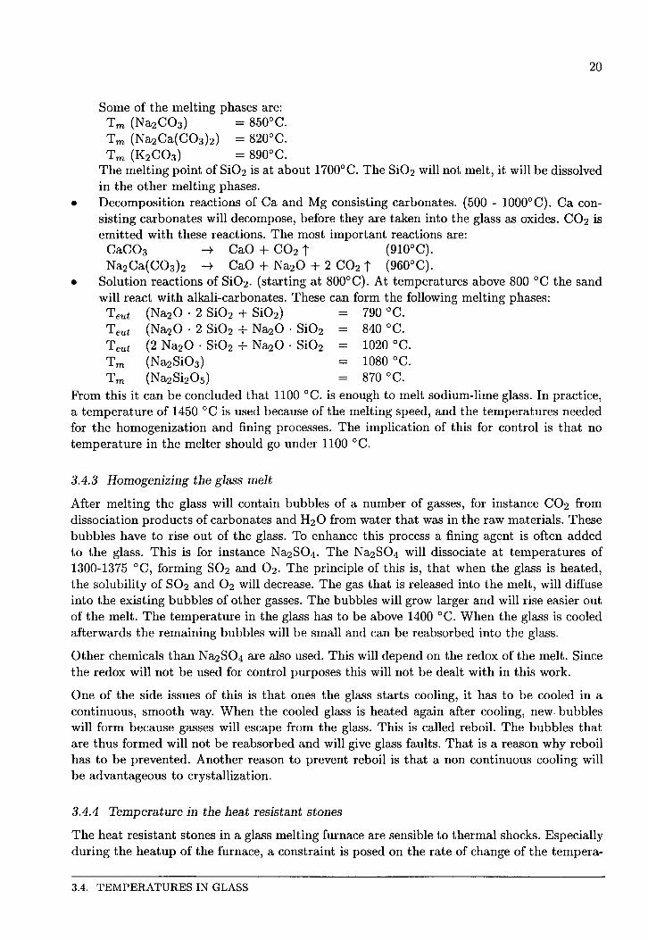
Some of the melting phases are: Tm (Na2C03) = 850°C. Tm (Na2Ca(C03)2) = 820°C. Tm (K2C03) = 890°C.

20

The melting point of Si02 is at about 1700°C. The Si02 will not melt, it will be dissolved in the other melting phases.

• Decomposition reactions of Ca and Mg consisting carbonates. (500 - 1000°C). Ca con­sisting carbonates will decompose, before they are taken into the glassas oxides. co2 is emitted with these reactions. The most important reactions are:

CaC03 ~ CaO + C02 t (910°C). Na2Ca(C03)2 ~ CaO + Na20 + 2 C02 t (960°C).

• Solution reactions of Si02. (starting at 800°C). At temperatures above 800 oe the sand will react with alkali-carbonates. These can form the following melting phases:

Teut (Na20 · 2 Si02 + Si02) = 790 °C. Teut (Na20 · 2 Si02 + Na20 · Si02 840 °C. Teut (2 Na20 · Si02 + Na20 · Si02 = 1020 oe. Tm (Na2Si03) = 1080 oe. Tm (Na2Si20s) 870 oe.

From this it can be concluded that 1100 °C. is enough to melt sodium-lime glass. In practice, a temperature of 1450 oe is used because of the melting speed, and the temperatures needed for the homogenization and fining processes. The impHeation of this for control is that no temperature in the meiter should go under 1100 °C.

3.4.3 Homogenizing the glass melt

After melting the glass will contain bubbles of a number of gasses, for instanee C02 from dissociation productsof carbonates and H20 from water that was in the raw materials. These bubbles have to rise out of the glass. To enhance this process a fining agent is often added to the glass. This is for instanee Na2S04. The Na2S04 will dissociate at temperatures of 1300-1375 oe, forming S02 and 02. The principle of this is, that when the glass is heated, the solubility of S02 and 02 will decrease. The gas that is released into the melt, will diffuse into the existing bubbles of other gasses. The bubbles will grow larger and will rise easier out of the melt. The temperature in the glass has to be above 1400 °C. When the glass is cooled afterwards the remaining bubbles will besmalland can be reabsorbed into the glass.

Other chemieals than Na2S04 arealso used. This will depend on the redox of the melt. Since the redox will not be used for control purposes this will not be dealt with in this work.

One of the side issues of this is that ones the glass starts cooling, it has to be cooled in a continuous, smooth way. When the cooled glass is heated again after cooling, new. bubbles will form because gasses will escape from the glass. This is called reboil. The bubbles that are thus formed will not be reabsorbed and will give glass faults. That is a reason why reboil has to be prevented. Another reason to prevent reboil is that a non continuous cooling will be advantageous to crystallization.

3.4.4 Temperature in the heat resistant stones

The heat resistant stones in a glass melting furnace are sensible to thermal shocks. Especially during the heatup of the furnace, a constraint is posed on the rate of change of the tempera-

3.4. TEMPERATURES IN GLASS

21

ture. At higher temperatures this becomes less important because the coefficient of expansion of heat resistant stones, for instanee silica stone, is smaller in this region. No information about a rate constraint on the temperature in operation conditions is found. For the MPe experiments, the rate constraint from the heatup is used. This is 25 oe per hour (taken from [26]) for temperatures over 1100 oe.

Another reason for being careful in changing the temperature is that changes in temperature may disturb the convective glass currents. This may lead to mixing of boundary layer of the glass next to the heat resistant stanes into the melt. These boundary layers are rich with contaminations from the heat resistant stones. This is because the heat resistant stone slowly melts into the glass.

The melting point of silica stone is about 1600 oe. This stone is aften used for building the roof of the furnace, because the molten silica does not contaminate the glass to much. The melting temperature is thus a high constraint on the temperature.

3.4.5 Conclusions drawn Erom temperatures in the glass melt.

From the temperatures and temperature regions in the glass a number of conclusions con­cerning the constraints for the MPe controller can be derived. First of all there is the low constraint arising from the liquidus temperature. Since this work only concerns the melting operation, this can betaken as a low constraint for all the temperatures in the furnace. Next there is the high constraint posed by the melting point of the furnace roof (the crown). This is a high constraint for all the temperatures in the furnace. A rate constraint is put on the change of the crown temperature by the dilatation of the heat resistant stones.

For the glass melt itself other constraints can be derived. The temperature from the hotspot in the glass melt to the throat has to descent as continuous as possible to prevent reboil. The temperature near the place where the batch is charged into the tank will have to be higher that 1100 oe for the batch to actually melt. Last, the temperature difference between the hotspot and the cooler regions of the furnace has to be big enough to maintain the free convective currents. In the result chapters, these conclusions will be applied.

3.5 Glass faults.

Different kinds of glass faults can be distinguished. Some of these, those that are related to unsatisfactory mixing in the tank, are:

• Stones. • Bubbles. • eords.

Stanes can have a number of causes:

• Insufficient melting. • Origination of christal from the molten glass. • eorrosion of the heat resistant materials like; melting of the crown, corrosion of the metal

line or furnace wall. erystallization round particles from the furnace wall.

CHAPTER 3. GLASS MAKING AND THE GLASS MELTING FURNACE

22

The first two causes can be opposed by a stabie and even temperature distribution, where the temperature is sufficiently high. For cause three the temperature should not be too high. The composition of the glass is also of concern to this. From control point of view stanes are mainly countered by good temperature distribution, because the composition of the glass is probably a fixed value.

Bubbles farm in the glass because gaseaus products of the melting and fining reactions have nat escaped form glass. This can be because the bubbles were nat big enough to rise farm the melt, because nat enough fining agent was added, or the fining agent did nat work because of insufficiently high temperature. It can also be because bubbles form through reboil of the glass. This kind of glass fault is dependant on the temperature distribution and on the amount and kind of fining agent.

Cords farm through inadequate mixing of the glass. The temperature distribution, bubbling and finingagent are important to this.

3.6 Measuring at a glass furnace

Because the furnace atmosphere is very aggressive and the glass is very hot, there are very little sensors available to measure properties in the glass. Normal sensors will dissolve in the glass melt. The result of this is that little measurements are done on a glass melting furnace. On some furnaces temperatures of the glass in the throat are measured in the heat resistant stanes next to or under the glass. In other furnaces the therma-couples have degraded and give very bad measurements. Among other properties that would be interesting to measure are the raw material content, the redox of the melt and the partial oxygen pressure. Work is being done to make sensors for these measurements, but in most furnaces no measurement is being performed. It will be an interesting topic for future research to look into the control aspects of this. It is nat treated in this work.

3. 7 Status of meiter control

Very little has been published on glass meiter controL Although people at TNO-TPD materials department report that some attempts have been made no applications of MPC are presently known of. The few references I found are listed in this section.

Wertz, Gevers and Sirnon [45] published an artiele on an adaptive GPC controller for bottorn temperature control of a glass meiter at the Glaverbel company. In the artiele, the perfor­mance of this controller was reported to be a significant improvement. Robert Bauer told me this controller was later abandoned because of poor results. At the Advanced control for industrial glass melters workshop (Appendix A) no mention of this project was made, although two of the writers of the artiele were present, and MPC controllers were discussed extensively. I spoke with Mr. Wertz at this occasion. He assured me the application was quite successful. His remarks about my work were that he expected that neural networks would nat be applicable because insufficient data would be available. He did expect promising results from multivariable control of the crown temperature.

3.6. MEASURING AT A GLASS FURNACE

23

TNO-TPD has made an inventory of the present control situation at glass companies [1]. The information was basedon questionnaires send to glass companies. The present control situa­tion at most companies is mainly based on manual control of steady state, stabie conditions and on procedures for adaptations, job or color changes. The crown temperature is controlled with PID control on the fuel/ air conditions. The bottorn temperature is monitored. At some companies, tests have been performed with other controllers. Vereenigde Glasfabrieken and Maasglas tested fuzzy control as an advisor for the operator. The Glaverbel GPC controller was also used at Maasglas, but found unsatisfactory. People at Maasglas think the cause for the failure of MPC and GPC experiments is that not enough input parameters have been taken into account. The report itself states that the failure is probable due to ill commu­nication with operators. Recent successes of fuzzy-logic based feeder control from Siemens company have arroused the interest of the glass industry for other fuzzy-logic based controL

CHAPTER 3. GLASS MAKING AND THE GLASSMELTING FURNACE

24

3.7. STATUS OF MELTER CONTROL

Chapter 4

Linear and Non-linear identification

During my work on the identification of the simulated glass melting furnace the following problem has arisen: How can I design an experiment that will be 'persistently exciting' the system, that will sufficiently span the input and output space, and that will excite the right frequency range, to make a dataset for the training of a dynamic neural network. At this there was a very serious limitation in the number of experiments and the size of data sets, due to limited computation facilities.

In neural network theory little or no attention is paid to experiment design. All neural network specialists agree that training data is essential to the succesfull training of a network. Most work however, to make the right data set, is put in getting the right data points from a large, previously reearcled data collection. Careful design of an experiment to create a dedicate data set is hardly ever clone. One reason for this is that most neural network applications are nat of a dynamic nature, so the sequence of data is nat important. Secondly, in some industrial neural network applications for model based control, a large collection of operation data is indeed available ([38]). In those cases, makinga data set, which is a time consuming operation that might very well put an expensive plant out of normal working conditions, would be a waste. In our own group Wim Bouman has previously clone some work on experiment design for dynamic neural networks [3], this will be one of my starting points.

First I will describe what assumptions are made for the topology of the neural network to be trained. In the same paragraph I will also explain what type of non-linear system, and what type of system operation I assume. In system identification theory the emphasis in the design of experiments is on designing an experiment for linear model identification. A popular signal is the PRBS (Pseudo Random Binary Sequence) signal. In the paragraph on linear identification I will describe the reason for this, also writing what argument carries over to the neural network case. Next, some signals proposed by other members of the Hybrid Modeling Group will be treated and based on those, a final experiment design will be presented.

4.1 Assumptions.

For the reason of keeping it simple, the most camman dynamic neural network type around is assumed. This is the feedforward neural network, made dynamic by using previous network inputs and previous network outputs as the network input. lt is trained as a prediction model and prediets one step ahead.

Obviously, the nature of non-linearity of the system to be modeled is important to the experi­ment design. The first assumption is that the system is time invariant, that is that fora given system history, and a given system input, the system output does nat depend on absolute

25

26

time. Next we assume the system output to be continuous. Also it is assumed that the static values of the system are monotonous. The result is not a very strong non linearity, but one that fits the non-linear systems we are studying. Some special cases of non-linear systems that we had in mind: a) a system in which a static gain is dependant on the magnitude of one of the inputs. b) a system in which a time-constant is dependant on the magnitude of one of the inputs. c) a system with hysteresis. To clearly explain the things we are doing we use a system with 2 inputs, so we eau actually span the input along more that one direction, and 1 output. The aim of this study is to obtain a model that eau simulate a system in a broad inputjoutput range.

4.2 Linear identification and modification for identifying neural networks.

In control engineering a system is said to be linear if the response to a linear combination of signals is the same as the same linear combination of the output responses of individual inputs. ldentification of systems that are believed to be sufficiently linear usually have the following steps:

• Talks and observations to obtain the smallest and largest time constants, input and output ranges and operating points.

• Free run experiments to find noise level and to estimate the system gain. • Step experiments to obtain gains and to verify the largest time constauts and settling

times. • Staircase experiments to verify the linearity of the system. • PRBNS (Pseudo Random Binary Noise Sequence) experiments for parameter estima-

tions.

For a non linear system with properties as described in the previous section, the first 4 experiments eau be the same. PRBNS signals however are not suited for identifying a neural network.

The reasou for using PRBNS signals in the first place are stemming from the assumption of linearity. PRBNS signals have a constant spectrum for frequencies up to f = ljTc , where Tc is the PRBNS characteristic time. Furthermore they are persistently exciting for infinite order. The foremost thing the experiment focuses on is to excite a brought range of frequencies. The amplitude of the signal is not important since a linear system is assumed. The most important frequencies are the ones round the bandwidth of the system to be identified. Very high frequencies are not important, since most common systems act as low pass filters and have a very low gain for high frequencies. Power is taken from this frequency region by adjusting the PRBS characteristic time. Very low frequencies are not important either, since when a controller is applied, added integrating feedback action will take the system to setpoint anyway. These frequencies are often removed by applying a high pass filter. Last PRBS is a zero-mean signal. For identification in a setpoint this is advantageous, because system output of a linear or nearly linear system will stay around the setpoint value.

For non-linear systems some of these arguments no longer apply. The amplitude becomes important. One of the most fundamental non-linearities, when moving away from the linear situation is that a steps of different size don't yield proportional results. The logical thing to do is to use a random step size. This yield a random signal. This is often implemented by

4.2. LINEAR IDENTIFICATION AND MODIFICATION FOR IDENTIFYING NEURAL NETWORKS.

27

calculating a random value for every input sample. The resulting signal has similar properties to zero mean white noise.

Secondly the lower frequencies become more important. Especially when generating data to train a neural network it is important to have the system reach it's final static value. Often this property is formulated as the need to span the input and output space of a system. In linear system theory, these values are reached through superposition of inputs. In neural networks, the final values have to be an actual part of the output domain of the data set, else they may not be part of the output space of the neural net, or values would have to be reached through extrapolations, which could be very poor. To illustrate this I will give the two extreme examples.

Imagine a neural network which approximates a linear relationship between the input and the output with one neuron sigmoid. A training algorithm will place the neuron with its central linear part along the training data points. The curved and saturated parts will end up far away from the data points, thus giving a near-linear extrapolation for values just outside the data range.

Next imagine a neural network which approximates a curved relationship between input and output with a lot of sigmoid neurons. Though there is no general rule for the way the neurons will end up, it could very well be that the neurons will each fit a small part of a curve. This will yield a near constant value for points just outside the data range.

All signals treated up to now were zero mean signals. As noted before this is advantageous because a linear model is only supposed to work in one working point. When one wants to identify a neural network in a working point, this still applies. When one wants the network to be able to simulate system behavior in a broader input and/or output range it may be necessary to use a signal that has a non-constant mean, that is, that has a different mean for pieces that have a length of at least the settling time of the system, and thus spans the input space. This guaranties that the output will also have a broader range and spans the output space better.

4.3 Derivation of some experiment designs.

For no apparent reasou ( except for the natural tendency of the mechanica! engineers in our group to use multi-sines) we started out using multi-sine signals for identifying neural­networks. Quite soon however this was questioned, for a multi-sine signal is persistently ex­citing to the order of two times the number of sine frequencies used. Persistenee of excitation is, in this case, formulated as the number of independent parameters of a model one eau maximally determine from a signal (the more precise formulation is somewhat different, see for instanee [20]). A sine has two adjustable parameters, the amplitude and the phase, and from an output signal resulting from a sine one eau thus determine two parameters.

A neural network has a lot of independent parameters. For the used feedforward network these number Nu* Nn + Nn + Nn * Ny + Ny, where Nu is the number of input neurons, Nn is the number of hidden layer neurons and Ny is the number of output neurons. Note that the number of input neurons is not the same as the number of system neurons, since both the system input and system output are fed to the network with a tapped delay line and

CHAPTER 4. LINEARAND NON-LINEAR IDENTIFICATION

28

thus result in a larger number of input neurons. In this way a small two input, one output system, with the inputs delayed one time (giving two times two network inputs) and output delayed two times (resulting in two network inputs), for a total of six network inputs. With six hidden neurons and one output this gives 54 independent parameters. This means using 27 different sine frequencies and leads me to conclude that it is easier to design a persistently exciting experiment by using signals which are persistently exciting for infinite order.

One of the things one can do to design a signal that has all the properties mentioned up to now is to combine a slow varying signal with a white noise signal. This results in signals like a staircase with noise superimposed and a sine with noise superimposed.

Another way to reach a signal is to have a superposition of a number of PRBNS like signals. A signal that looks particularly nice is one that has a PRBNS with large Tc and large amplitude added to a second PRBNS which has a smaller Tc and a smaller amplitude added again to a third PRBNS with again smaller values. Insteadof using a binary signal, like PRBS, as bases, we used a signal with three levels. We called the result a QPRTS signal (Quantisized Pseudo Random Trinary Signal). In figure 4.1 this is graphically shown.

The signals proposed in this section were tried on a non-linear test system by Patriek Stapel [34]. Next they were examined for inputfoutput spanning and dynamic spanning by studying the inputfoutput space of the system. The system had the output delayed two times, and no delayed inputs, giving a four dimensional input space. The QPRTS performed best, the staircase with noise second best. Agnes van Oasterurn took these results and used all kinds of signals for network identification [43]. Again QPRTS was best. For this work the QPRTS signal was used as an experiment design for identifying the multi output linear model and the neural network model of the glass melting furnace.

4.3. DERIVATION OF SOME EXPERIMENT DESIGNS.

29

10

I 0

I -10 0 10 20 30 40 50 60 70 80 90 100

10

0

-10 0 10 20 30 40 50 60 70 80 90 100

10

0

-10 0 10 20 30 40 50 60 70 80 90 100

20

0

-20 0 10 20 30 40 50 60 70 80 90 100

Figure 4.1: From above, first three components for a qprts signal, and last the three parts added toeach other giving the resulting QPRTS.

CHAPTER 4. LINEARAND NON-LINEAR IDENTIFICATION

30

4.3. DERIVATION OF SOME EXPERIMENT DESIGNS.

Chapter 5

ldentification of the Glass Tank Model (GTM) of TNO-TPD

In this chapter the methods foliowed to derive a model for the model predictive controller is presented. The Glass Tank Model (GTM) is examined for non-linear behavior. Next a linear model with one controlled input, one uncontrolled (disturbance) input and one output is identified. After that a bigger linear model is derived with three controlled inputs, one uncontrolled input and nine outputs. Last a neural network is trained. As a condusion the expectations for the controller will be formulated. The methodology for linear rnadeling was taken form E. Weetink [44]. Linear rnadeling theory was stuclied from the PATO course on process identification [42], L. Ljung [20] and Van den Bosch and Van der Klauw [41].

5.1 The glasstank model

A three-dimensional mathematica! GlassTank Model has been developed by TNO-TPD for the description of heat transfer, glass flow and chemica! reactions in glass tanks. This model uses a glass flow model as a base. To predict the glass quality a lot of extra information is required with respect to melting kinetics, redox and (re)fining, bubble tracing (including bubble growth, shrinkage and change of composition), homogenizing, corrosion of refractory, heat transfer, combustion, batch blanket behavior, foam behavior, volatilization and residence time distribution.

The model is being used for trouble-shooting, process optimization and designing of new glass tanks. It is capable of performing simulations for very different types of glass tanks. Forced bubbling, electrical boosting, flow harriers and so on, can be involved.

The mathematica! form of GTM is a finite differential model. The input to GTM contains a grid of points, in which the temperatures and other properties will be calculated. The model will forma second grid of points in between the main grid in which other properties like the partiele velocity and the heat transfer are stored. Each cell in between the grid points can contain a materiallike glass, wall or surroundings. For a more detailed description, one should contact TNO-TPD.

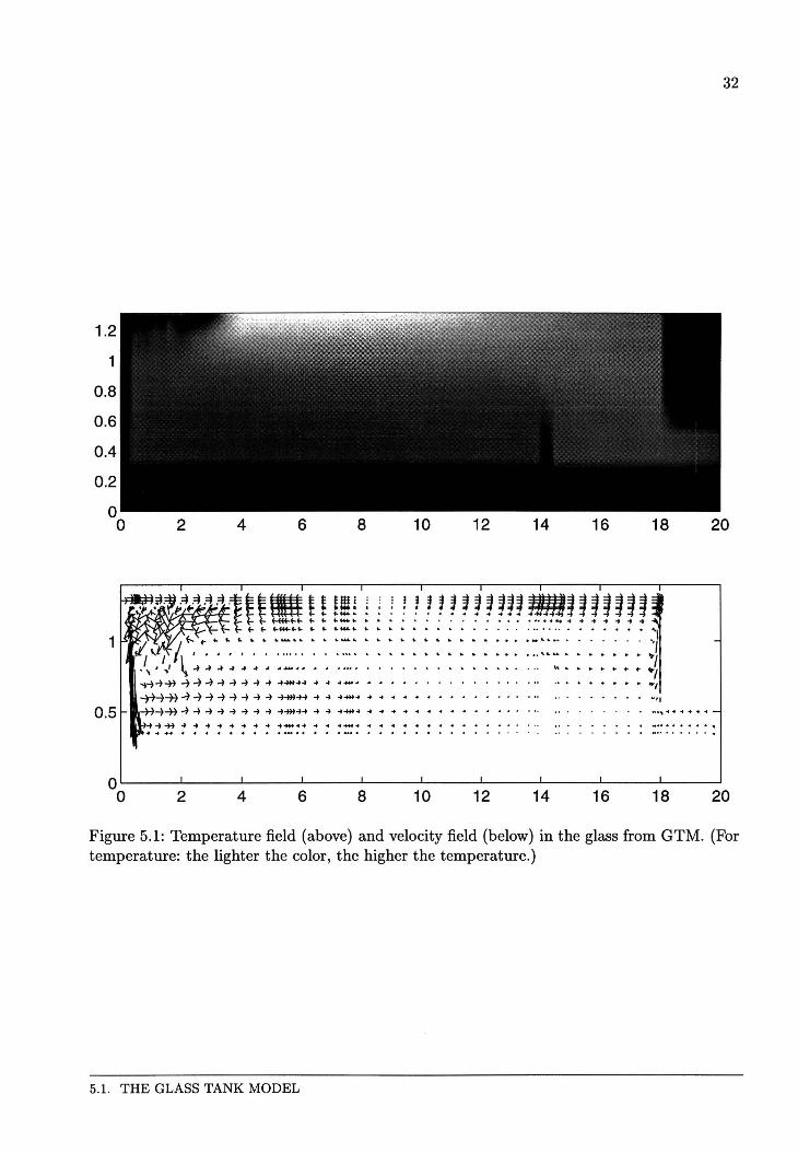
For this work, a two dimensional version (three cells deep in the dimensionless coordinate) was used, to reduce calculation time. In figure 5.1, a plot of the temperature and velocity field as calculated by GTM are shown. A sample input file is in appendix B.

31

1.2

1

0.8

0.6

0.4

0.2

0 .5

2 4 6 8 10

-+~ ... ~ ............ -t+t+ .............................. . .. .. .... .. .. . .. . .. .. .. ........... . . ..... . . . . . . . . .

32

12 14 16 18 20

.. . .. ,.

0~----~----~----~----~----~----~----~----~----~----~

0 2 4 6 8 10 12 14 16 18 20

Figure 5.1: Temperature field (above) and velocity field (below) in the glass from GTM. (For temperature: the lighter the color, the higher the temperature.)

5.1. THE GLASS TANK MODEL

33

5.2 First examination

Normally an identification process starts with talks with operators to determine things like the smallest and largest time constant of the system, normal operating points and ranges of inputs and outputs. U nfortunately no operators are present on a computer simulation, so I had to do with comments in literature and the knowledge present at TNO-TPD. From this I knew that time constauts in the glass furnace would range from seconds for the control actions, through minutes for crown and flame temperature , to hours or even days for the currents in the glass and the glass quality. The glass furnace was described to he very non-linear.

For my simulations the time constauts in the range of seconds and minutes were neglected and the associated actions presumed instant. That way I had the crown temperature as a direct input {and not the fuel rate which is often the input at real furnaces). The throat temperature {Tl) was the logical output tolook at. The next step was to choose a sampling time. Choosing a larger sampling time would mean that the calculations of GTM would he shorter sirree a larger sampling time needs comparatively less iterations. A shorter sampling time would enable a closer examination of the output. A sampling time of 15 minutes was found to he a good trade of. The calculation of one hour of furnace time cost about 6 minutes of real time giving a ratio of 1:10.

The first experiments dorre, were free run and step experiments. These showed that the settling time of the furnace was about 100 samples {25 hours of furnace time). The biggest time constant was estimated to he around 30 samples (7.5 hours of furnace time).

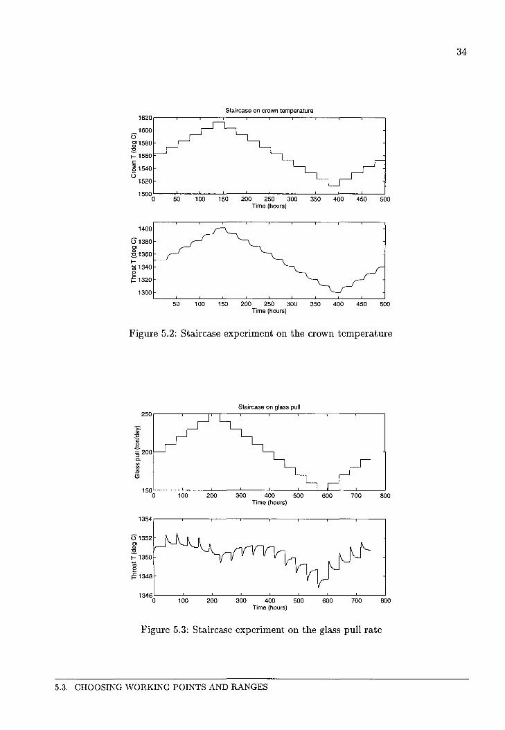
Now staircase experiments could he dorre. The results of these experiments can he seen in figure 5.2 and figure 5.3. The condusion of these were, that the non-linearity of the furnace was not that bad, and that the non-linear behavior was mainly of a static nature.

The furnace geometry used for the simulations is shown in figure 5.4. lts length is 20 m, of which 17.8 m is glass and the rest wall or throat. lts width is 6 m {this is not simulated of course, except for boundary conditions). The glass is 1 m deep. The glass pull for which it was designed is 200 tonsfday. The height of the throat is 25 cm. There is a flow harrier at 14 m from the melting end, which is 0.4 m thick and 0.85 m high. The grid consists of 73 points in the lengthof the furnace and 18 in the height. In the dimensionless direction, there are 3 cells, one for calculations and two for boundary conditions. In figures other than 5.4 the sealing of height and lengthare different.

5.3 Choosing working points and ranges

The working point of the glass furnace and the ranges of the input and output values were determined in meetings with Robert Bauer and Marc de Jongh. As a working point, the steady state value of the model, when when it was delivered to me, was chosen. The working ranges were chosen to match the changes that might occur in a real furnace. For the crown temperature, the highest temperature of the crown is used. The real temperature of the crown is a profile with the highest temperature over the hotspot. When changes are made on the crown temperature, the whole profile is changed by the same difference. The working point and ranges are given in table 5.1. Additional to the given range of the glass pull an extra change in the pull for job changes would he studied. This is a temporary reduction of the pull by 50%

CHAPTER 5. IDENTIFICATION OF THE GLASSTANK MODEL (GTM) OF TNO-TPD

34

Staircase on crown temperature 1620

1600 ü g>1580 :s f- 1560 c: ~ 1540 ü

1520

1500 0 50 100 150 200 250 300 350 400 450 500

Time (hours)

1400

Ü1380 Cl

:S. 1360 f-til 1340 e r= 1320

1300

50 100 150 200 250 300 350 400 450 500 Time (hours)

Figure 5.2: Staircase experiment on the crown temperature

Staircase on glass pull 250

>: "' ::!2 c: g '§ 200 c.

"' "' "' a 150

0 100 200 300 400 500 600 700 800 Time (hours)

1354

Cl Q)

:s f- 1350 til e r= 1348

1346 0 100 200 300 400 500 600 700 800

Time (hours)

Figure 5.3: Staircase experiment on the glass pull rate

5.3. CHOOSING WORKING POINTS AND RANGES

35

17.8m

0.55m! o 0.25mt

20m

14m

Figure 5.4: The furnace geometry

Input Associated primacs variabie working point working range erown temperature TeROWN 1563 oe 1500-1600 oe Glass pull PULLIN 200 ton/day 180-220 tonfday

Table 5.1: Working points and working ranges .

. This kind of dip will occur when machines for bottie or pot fabrication are changed. The deviation on the setpoint temperature that would be sufficiently small for further processing was chosen to be 3 oe. In the start ofthe project, changes in raw material composition were also studied, but this case was later drop because of poor performance of GTM for this kind of calculations.

5.4 Linear identiE.cation of the single output model.

The parameter structure used to identify a linear model is the OE (output error) structure because OE models offer the better model for doing simulations when compared to ARX and ARMAX models. The OE structure is:.

B(q) y(t) = F(q) u(t- nk) + e(t).

With nk the number of samples dead time and,

(5.1)

(5.2)

(5.3)

The polynomials B(q) and F(q) are found by minimizing the squared sum of errors e(t) for a suitable data set. The experiment used was a PRBS experiment. A part of this signal is shown in figure 5. 5.

The amplitude was chosen to be 20 oe for the crown temperature and 20 ton/day for the glass pull. The basic period of the PRBS signal was one sample (15 minutes). Identification was clone with the PEM (prediction error method) function of MATLAB. nb and nf were both chosen 4, for the crown temperature as well as the glass pull. Higher orders did not

CHAPTER 5. IDENTIFICATION OF THE GLASSTANK MODEL (GTM) OF TNO-TPD

36

PRBS on crown temperature ~1590 u ~1580

r-

Ql z 1570 I!! Ql

~1560 .al ~ 1550 ~ "1540

25 30 35 40 45 50 Time (hours)

1348

~1346 u Cl

~1344

1338 '-------'------'-----.L..------'--------' 25 30 35 40 45 50

Time (hours)

Figure 5.5: PRBS experiment on the crown temperature

result in better identification while lower order would have difficulty to find a good solution. nk was found to be 1 (i.e. no dead time). The OE model was converted to a state-space model using MATLAB. This state space model was used in the MPC module of primacs. For model validation, a number of methods were used. The resulting data was simulated with the training data as input (auto validation), and with data from other experiments. The frequency domain response was also examined, by camparing ETFE (empirica! transfer function estimates) estimates of experiment data and bodeplots of the identified OE models. Figure 5.6 shows the auto validation of the crown temperature. Figure 5. 7 shows the cross validation of the crown temperature model on a staircase experiment. Though this is not a very good methad of validation~ the amount of non-linearity can beseen very clearly.

5.5 The multiple output model.

The glass industry has suggested that the proposed MPC controller should control the glass quality rather than just the throat temperature. In chapter 3, a number of factors important to the quality of glass have passed. To translate this into constraints for the MPC controller a number of monitoring points important to the furnace operation had to be found. In figure 5.8 these points are shown.

5.5. THE MULTIPLE OUTPUT MODEL.

37

15,-------.--------.-------.--------.-------.-------~

10

5

0

-5

-10

-15L-------~-------L------~--------~------~------_J

0 500 1000 1500 2000 2500 3000

Figure 5.6: Auto validation of the crown temperature.

Gomparisen between measured staircase and simuialed staircase 60,--------,---------,--------.---------.--------.

40

ü g> 20 E c:

~ ~ 0 E _g c: ~ ~ -20

-40

-WL-------~---------L--------~--------~------~ 0 500 1 000 1500 2000 2500

Time (samples, 1 sample= 15 minutes)

Figure 5.7: Staircase experiment compared to simulated data.

CHAPTER 5. IDENTIFICATION OF THE GLASSTANK MODEL (GTM) OF TNO-TPD

38

CT1 CT2 CT3 0.0 5.0

. I::;

"-

8 iTI7

Figure 5.8: The temperature points in t he glass furnace

temperature coordinate description Tl 70x 04y Throat temperature: the main temperature to be controlled.

Sametimes measured. T2 30x 04y Bottom temperature in the middle of the furnace.

Sametimes measured. T3 05x 04y Bottom temperature at the melting end.

Sametimes measured. T4 05x 16y Temperature directly under the batch blanket.

Important to melting rate. T5 30x 16y Hotspot temperature. Important to proper homogenization. T6 45x lOy Fining area temperature. Important to proper circulation. T7 70x 02y Measurement in wall, derived from Tl.

No further use in this work. T8 30x 02y Measurement in wall, derived from T2.

No further use in this work. T9 05x 02y Measurement in wall, derived from T3.

No further use in this work.

Temperatures Tl, T2 and T3 were chosen because these are the temperatures that are most often measured in real glass tank furnaces. T4, T5 and T6 were chosen because the tem­peratures in these points have an actual meaning for the glass quality. T7, T8 and T9 were defined to provide the possibility to study the effect of indirect measurement on the glass furnace controL

With these outputs it was no longer sufficient to control just the crown temperature. To have more inputs, the crown temperature profile was defined as a spline function with eight section and nine division temperatures CTl upto CT9 (figure 5.8). Actually, this was the way GTM got its crown temperature all along, it was just not used for controL The link between primacs

5.5. THE MULTIPLE OUTPUT MODEL.

1 .

0.

0

39

and GTM had to be amended to use this control method. For the control cases I divided the nine temperatures in three groups. These sections will be called by the first temperature in each group; CTl, CT4 and CT7.

5.6 Identification of the multiple output model

For identification purpose a QPRTS experiment was clone (see chapter four). Simultaneously, four QPRTS signals were put on CTl, CT4, CT7 and PULLIN. This was used to perform a OE identification for the nine output temperatures. Again all orders were chosen to be 4. Figure 5.9 shows the auto validation of the fining area temperature {T6). Figure 5.10 shows the cross validation of the melting end bottorn temperature {T3). After identification, three extra outputs were made in the resulting statespace model. These were the differences between;

1. the hotspot and the fining area temperature {T5- T6), 2. the difference between the fining area and throat temperature {T6 - Tl), 3. the difference between the hotspot and the melting end bottorn temperature {T5 - T3).

The reason for this is that a low constraint on T5 - T6 and T5 - T3 will ensure temperature differences, the engine for the free convective flows. The difference T6 - Tl is added to be able to lay a low constraint to counter reboil. The resulting four input, twelve output model was put into the primacs MPC module.

5. 7 Training of a Neural Network

With the same QPRTS data as the previous model, a neural network was trained for the throat temperature. For training, the neural network training tool of Ron Hensen [13] was used. Training was done as a simulation model. The order of back coupling of the input and output signals were all chosen 4, and the network had 4 hidden neurons. The network topology was thus, 20 input neurons, 4 hidden neurons and 1 output neurons. This proved to be the minimum topology that was easy to train, withorder 3, training failed. Though training took very long ( about 1 day), the result was promising. The cross validation was better than that of the linear model. Due to lack of time, no MPC experiments were done with this network.

CHAPTER 5. IDENTIFICATION OF THE GLASS TANK MODEL (GTM) OF TNO-TPD

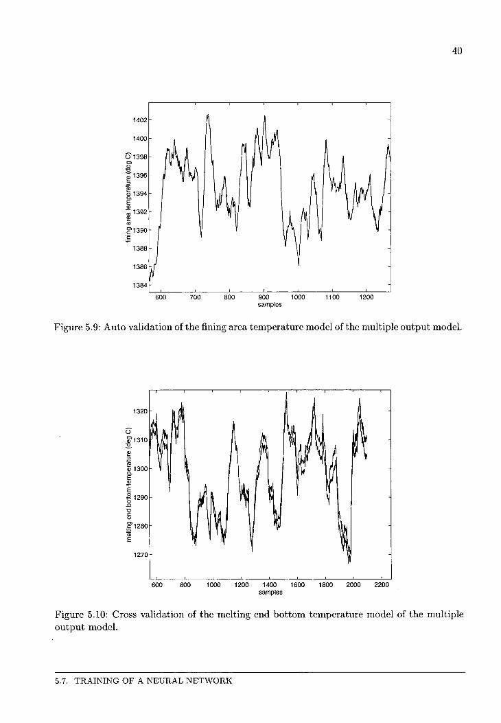
1402

1400

Û1398 Cl Q)

"C -;; 1396 :; (ij êii 1394 c. E Q)

-;;; 1392 2! "' g'1390 ·;:: ;;:::

1388

1386

1384

600 700 800 900 samples

1000

40

1100 1200

Figure 5.9: Auto validation of the fining area temperature model of the multiple output model.

1320 ~ û ~ ~ ~ ~ ~ al'1310 ~J 1\ :s 2! ~ \ ~ ~ êii 1300 c. E 2

~~ ~ E g 1290 0 .0 "C c:

' ~ Q)

§'1280

~ äi E

1270

600 800 1000 1200 1400 1600 1800 2000 2200 samples

Figure 5.10: Cross validation of the melting end bottorn temperature model of the multiple output model.

5.7. TRAINING OF A NEURAL NETWORK

Chapter 6

MPC simulations

In this chapter the results of the MPC simulations with the two linear models are presented. The results of the single output model are showed first. They show the basic MPC possibilities like making faster setpoint changes by oversteering, using constraints and adding feedback action to compensate for model faults. For the multiple output model the tuning of the MPC controller is discussed. After that, the control cases used for the multiple output controller are explained. When the results of these simulations are given, a comparison with the present control situation in the glass industry is made.

6.1 MPC experiments with the single output model

The simple, single output, output error model was used to test a number of the standard MPC features on the glass furnace simulator. This was clone based on the following three control cases:

• A change in setpoint for the throat temperature. • A sudden decrease of 50 % in the glass pull. This case arise from the fact that such

changes do occur in the container glass fabrication, when a machine for a new type of bottie or pot is connected.

• A change in the recycling cullet fraction of the batch. This case was based on the knowl­edge that the european glass industry uses a lot of recycling cullet as a raw materiaL This case was discarded because GTM was not able to do the needed concentration calculations on the 2 dimensional model.

For the tuning of the MPC controller a number of values have to he determined. These are:

fY The setpoint weight matrix. ru The control move weight. p The prediction horizon. m The control horizon.

The value of the prediction horizon has to he chosen bigger than the largest time constant. The value of the prediction horizon has to he larger than any inverse response or dead time. I used a prediction horizon of 75 samples and a control horizon of 20 samples. These are values that are larger than strictly needed. With the single controlled input, single output model, the weight matrices are scalars. Optional a number of constraints on the input and output can he defined. Figure 6.1 shows an MPC simulation of the setpoint change case with setpoint weight fY = 5 and ru = 1. The MPC willoversteer to reach setpoint faster. Figure 6.2 shows an example of the use of a high constraint. Figure 6.3 shows the effect of a move constraint. Notice that the controller does not steer the crown temperature to a high value

41

42

at once but will do so with a maximum of 1 oe per sample. Figure 6.4 shows closed loop MPe. In this case a first order filtered value of the difference between the actual output of the throat temperature Tth and the predicted output 'Î'th is added to the predicted throat temperature, compensating for model faults .

'Î'th(n + 1) = 'Î'th(n) + K(Tth- 'Î'th)· (6.1)

With K the filter constant. Thus the predicted output will eventually he the same as the actual output in steady state conditions. The errors in prediction of steady statevalues after setpoint changes of 20 oe was about 5 %.

Setpoint change on the throat temperature 1610

I~ ~1600 (.)

g>1590 :!?.. 1- 1580 c:

~ 1570 (.) --'

1560

1550 0 2 3 4 5 6 7 8 9 10

1365

Û1360 ------------i' 'C

;: 1355 Oi e f3. 1350

1345 0 2 3 4 5 6 7 8 9 10

Figure 6.1: Setpoint change on throat temperature controlled with an MPe controller. rY =

5,ru = 1 .

6.2 Control cases

The following control cases were defined for testing the multiple output model.

1. Throat temperature setpoint change. A step-like change in throat temperature setpoint will he applied. The controlled input of the process will he the crown temperatures. The control algorithms used will he: • Manual control (statie values applied at setpoint change). • MPe control with or without constraints, open loop. The constraints in the MPe case can he: • High constraint on crown temperature because of possible melting of heat resistant

blocks. • Rate constraint on crown temperature to prevent disturbance of pollution rich glass

near the furnace walls, because there are limits on the flame temperature and to prevent damage to furnace blocks due to thermal dilatation.

6.2. CONTROL CASES

43

Setpoint change on the throat temperature 1610.---,----.----.----.---,.---.----.----.----.---.

~1600 ü ~1590 "0

;::- 1580 c ~ 1570 ü

1560

1550L_ __ _L __ _i ____ ~---L--~L---~--~----L----L--~

0 2 3 4 5 6 7 8 9 10

1365.---,----.----,----.---,.---.----.----.----.---.

Û1360 Cl Ql :3. f- 1355

~ r= 1350

1345L----L---i----~---L--~L---~--~----L----L--~

0 2 3 4 5 6 7 8 9 10 time(hours)

Figure 602: Setpoint change on throat temperatureo High constraint on crown temperatureo Tmax = 1600ofY = 100,ru = 1 0

Disturbance in glass pull.

5 6 Time (hours)

Figure 6o3: Disturbance in glass pull. Move constraint on crown temperature b.Tmax = l.fY = 5, ru = 1 0

CHAPTER 60 MPC SIMULATIONS

44

2. Disturbance of throat temperature due to pull variations. A step-like change in the pull will occur. The throat temperature will be controlled in the same two ways as the in the previous case.

3. Ambient temperature variations and day /night cycle. This case was dropped due to limitations of the gtm/primacs interaction. Furthermore, the relevanee of this case is arguable. Glass technology experts will have to be asked for their apinion on the influence of ambient temperature on: • The furnace temperature due to heat loss through walls. • The furnace temperature due to batch temperature variations. • The glass composition due to batch composition variation. • Temperature disturbances like opening of inspeetion hatches. • Temperature variations due to seasonal variations.

4. Raw material and cullet ratio. Batch composition. This case was dropped because of limitation of gtm. The incorporation of concentration calculations is being worked on.

5. Temperature field regulation. General rules will be described for the temperature and the differences in temperature with the aim to: • Prevent current reversal. • Sustain melting rate. • Prevent reboil. • Prevent crystallization. The input for this will be the crown temperature profile.

6.3 Tuning the multiple output model

For tuning the values of the weights, the constraints and the horizons had to be determined again. A lot of these values could he taken directly from the previous experiments. The predietien and control horizon were chosen to be the same as before. From the experiments with the single output model it was known that the system response would be good if the ratio of the setpoint weights and the move weights would be 5. The constraints for the temperatures in the glass were taken from the theory in chapter 3.

Temperature Tl T2 T3 T4 T5 T6 CTl CT4 CT7

Low constraint 1200 1200 1200 1200 1450 1350 1350 1450 1350

High constraint 1500 1500 1500 1500 1600 1600 1600 1600 1600

Rate constraints (°C/sample)

5 5 5

The low constraints of the monitored temperatures were all chosen 1200 ° except for those temperatures that are in areas in which fining takes place. There higher values were taken. The high constraints of all temperatures were chosen 1600 except for measured temperatures that are near the wall (which are nearly all measured temperatures) there a lower value was taken. Finally a rate constraint of 5 ° / sample was applied to all controlled temperatures. To

6.3. TUNING THE MULTIPLE OUTPUT MODEL

45

prevent damage by thermal shocks. For the differences of some temperatures other constraints were chosen. This was difficult because no information or theory about these choices exists. In the end the values were chosen near the steady state values, to be able to show the ability of the MPC controller to control this.

Temper at ure Low constraint High constraint Reasou T5- T6 100 150 Ensure good convection, prevent reboil. T6- Tl 40 80 Prevent reboil. T5- T3 200 240 Ensure good convection.

6.4 MPC experiments with the multiple output model

The model was stuclied for controllability. In figure 6.5 the step responses to the three tem­perature inputs are shown for the four temperatures that were determined to be important to glass quality. In this the static gain matrix of the inputs can be seen. The gain matrix can be calculated with:

G = C(I- A)-1 B + D. (6.2)

This gives:

CTl CT4 CT7 PULLIN Tl 0.1526 0.2251 0.6239 0.0238 T3 0.7293 0.4598 0.2763 -0.7047 T5 0.1878 0.7272 0.0689 -0.1041 T6 0.3832 0.3712 0.3197 -0.3359

From these values it can be concluded that the four temperatures chosen as measurements for temperature field control can be independently controlled, because no row in the gain matrix is equal. This was very surprising because it was expected to be very difficult to control the temperatures in the glass furnace independently, due to coupled behavior.

At this point the experiments were done. At first only one setpoint was supplied to the controller. This resulted in the controller pushing the furnace out of the linearisation area, because one input was enlarged until the constraint was hit and another was decreasing pro­portionally. The drifting resulted in errors in the prediction of the throat temperature of 100 %. In the next experiments more setpoints were supplied to fix the furnace in its linearisation area. Especially giving a setpoint for T3 is effective. Tl and T3 are the temperatures most often measured on a regular bases in a real meiter, so supplying a setpoint for those point is not an unrealistic thing to do.

In figure 6.6, first a small change in the setpoint is made and afterward a change of 10 % is made in the glass pull. For the pull change, the controller is able to keep the furnace inside the 3 oe expectable margin round the setpoint.

In figure 6. 7 and figure 6.8 the effect of using constraints on the differences of temperatures is shown. With nearly the same response in the throat temperature, the drop in the temperature difference is one third of the drop with unconstrained MPC and half of the drop with manual controL A drawback is that the constrained situation takes the meiter farther away from the linearisation area and because of that has a bigger prediction fault.

CHAPTER 6. MPC SIMULATIONS

46

In figure 6.9 the MPe controlled situation is compared to the current method of control in the glass industry {making changes by supplying steady state values as step input). 1t can be seen that while in figure 6. 7 the meiter takes 8 hours to get back to within the 3 oe margin, in figure 6.9 the meiter takes 15 hours to do the same. lt should be noted that the MPe controller could be faster if no constraints would be laid on the rate of change of the crown temperature. Adding a feedback action would also lead to a faster reaction. The manual control had no rate constrained imposed on it.

6.5 Condusion

I this chapter it was shown that the throat temperature of glass melting furnace can be controlled with a linear MPe controller. The predietien error of the linear model will be dependant on the amount of deviation from the linearisation area. In the cases I stuclied it was not worse that 10 % of the deviation ( in the order of 3 ° e ) . The error on the control that results from this can be easily compensated by a feedback action. From TPD-glass we have heard that the margin of error acceptable to normal operation is in the order of 3 oe. The condusion is thus that a linear simulation is sufficiently accurate to be used for the control of a glass melting furnace. A MPe controller would be able to improve considerably on the present control situation. Using multi-variabie crown temperature control would be able to improve the glass quality control by preventing the causes for a number of glass faults.

6.5. CONCLUSION

47

Disturbance in glass pull.

r:r'----------'--F;:--'-------'----• ------'-------': J 0 2 4 6 8 10 12

i :~r'----------'--s;?:------'-------J--- ----- ------L_m--~ n :------'-------'--1 0 2 4 6 8 10 12

r~ c 180 g '5 160 0..

140 1

: : : : : : : : : : 1 2 3 4 5 6 7

Time (hours) 8 9 10 11

Figure 6.4: Disturbance in glass pull. Closed loop MPC. fY = 100, ru = 1 .

CT1 CT4 CT? 1.-----~--------~ 1.---------------·

i= 0.5 0.5 0.5 (

0 ----0 20 40 1.-------------~

~0.5( o~----~------~

0 20 40 1.-----~--------~

~ 0.5

o!r 0 20 40 1.------~----------,

~ 0.5

OI/ 0 20 40

0/ 0 20 40 1.-------------~

0.5 Î o~----~------~

0 20 40 1.-----~--------~

r 0.5

OL-------------~ 0 20 40 1.-------------~

0.5

OI! 0 20 40

OW-------------~~

0 20 40 1.---------------·

0.5

0/ 0 20 40 1.----------------~

0.5

0 l..:::::=:=========--_j 0 20 40 1.-------------~

20 40

Figure 6.5: Step responses of four temperatures to the three controlled crown temperatures

CHAPTER 6. MPC SIMULATIONS

48

1450

;. :

~1400b r 1350

'-----~1 1570°

50 100

~1560F ~ \ : 1550

150

----------.{ l 1500°

50 100

~1450k ~ •

1400

150

l 1380°

50 100

f= 1360~ :-\ ; ,-/ ,-....

1340 0 50 100

~:::t ; :

0 50 100 150 time(hours)

Figure 6.6: First a change in setpoint, later a medium step-like disturbance in glass pull.

i::t : Ç-· -: -l 80~--------~--------~--------~--------~------~

14500 5 10 15 20 25

E 14ool f----------.,: ~ : , : l 1350L_ ________ L_ __ ~==--~----=---~--------~------~

14600 5 10 15 20

~, .. af ; 1 , ; , j 1420~---------~---------~--------~--------~--------~-

25

13600 5 10 15 20 25

e: ::::r :0c_c ccc:c "" """ c~c """ cccJ 0 5 10 15 20 25

~ ::t \ : : : l 0 5 10 15 20 25

time(hours)

Figure 6. 7: Big disturbance in the glass pull. Difference temperatures are monitored.

6.5. CONCLUSION

49

i :::fL--_______.!____"----_-=---: -=--: __ ____...L..__.' =1 14500 5 10 15 20 25

6 ~:::IL-----L_: ~~: ---------'-----: -------'---: _l 14600 5 10 15 20

8 1«+ ' / : : : 1 1420~----------L·---------L--------~--------~--------~-

1360~ 5 10 15 20 25

~ ~:::CL---···· ·_______.!____: G_--~ .~. ~ · ~____.________-< ~ --____.___~ -~ ~---- ~ -~_____._____~ ~ ~ ~ -_~ --1 0 5 10 15 20 25

25

~ ~=t \ ' : : J 0 5 10 15 20 25

time(hours)

Figure 6.8: Big disturbance in the glass pull. Constraint on difference temperatures.

i :::fL--_______L___: ----_ -_....!..____: -=:-=--=: ~1 0 5 10 15 20 25

E 14001 ~ : : : I

1350~--------L---------L---------L---------~------~

1460(} 5 10 15 20

8 ::::f i : : : l 25

1360(} 5 10 15 20 25

>= ::+ ........... : Cii~ ~-~~cc~ _c c_c ~~cc _c ~""l 0 5 10 15 20 25

<::[ \ : : : 1 0 5 10 15 20 25

time(hours)

Figure 6.9: The same disturbance as the last experiments, with present controL

CHAPTER 6. MPC SIMULATIONS

50

6.5. CONCLUSION

Chapter 7

Con cl usions.

In this chapter a number of condusions about the various aspectsof this work will be made. Generally speaking, the first condusion should be that this research is not complete. Most condusions will be foliowed by a recommendation.

7.1 About model predictive control and neural networks.

When I made my way through the different MPC methods it became dear to me that although MPC is a nice, practical way to control chemical plants, there is no general theory descrihing the method, especially with nonlinear models. The absence of a standard textbook illustrates this. This makes a good mathematica! analysis of the combination of neural networks and MPC difficult. The results of others are very promising but still a lot of work has to be done. The lack of implementation of a combination in this work makes an objective condusion impossible. It should be remembered however that a MPC controller is only as good as its model. Adding feedback or adapting action, for instanee a Kalman filter approach can help, but will result in loss of performance if the plant has to be operated doser to setpoint then the model error.

The methods at hand to use neural networks for dynamic system simulation are getting better. The differences between methods and vocabulary of the neural network and the control community are very big however. A systematical experiment design can not be found in literature. For the glass furnace it was found that a neural network is not needed to make a good model predictive controller.

7.2 About the control of glassmelting furnaces.

There is a lot undear about the nature of dynamica! behavior of glass melting furnaces. Where people from the glass industry say that a glass melting furnace is highly nonlinear, control community people (like mr. v/d Braak at the advanced control workshop) have sametimes said that the nonlinearity of the glassmelting furnace is not that bad. There could be reasons for this. It could be that the nonlinearity meant by the glass people is a static nonlinearity. In that case, control people would be speaking of a dynamic non-linearity. It could also be that the control people have not looked into the matter deep enough to have seen al different operating conditions and disturbances.

The glasstank model I investigated was not that nonlinear. It could be that TNO-TPD gave me a special furnace that was more stabie than most furnaces, to make my life easier, or the calculation time shorter. In that case many condusions of this report could be wrong.

51

52

7.3 About the linear MPC controller.

The linear MPC controller was shown to be able to control a glass furnace to within the demanded precision. Along with that, a number of aspects of glass quality could be controlled at the same time. In cases were setpoint changes are made, the temperatures of the furnace can be brought within the demanded working range upto three times as fast. lt can be concluded that this would also apply to events like color changes. More experiments are needed to make more quantitative statements about this.

7.4 About the primacs model predictive control implementation.

The primacs MPC implementation showed to be a reliable MPC implementation. It caused me a lot of trouble however, befare getting it to work properly. The lack of a good manual on the importing of linear models into the primacs format (which was at the start the MATLAB format, very convenient, until MATLAB changed its data format), and on writing new model structures, is part of the reason. The dated graphical interface (the new one is nearly ready) was another. It worked fine with a small number of variables, but with the twelve output model, I completely lost my way. It was for instanee nat able to display all states of my model at the same time, because the window in which this would be displayed could nat be scrolled. I would gladly lend my experience to help make a new MPC interface.

7.5 About the glasstank model

GTM also worked fine, when the settings and options were right. It took until December 1997 however to get that far. Partly because it was assumed that the linking with primacs was ready to be used at the beginning of my project, it was nat clear until very late that sarnething was wrong. I did nat get a proper manual until august. At the same time, the concentration experiments were dropped because the calculations showed numerically bad results. In September, it became clear that the boundary conditions had been wrong all along. It took until October befare changes were made on the interfacing with primacs to use multiple crown temperatures, because the GTM people were toa busy until that time.

The main problem, in my eyes, was that the evaluation of the interfacing between primacs and GTM was nat part of the project description, which led me to believe I would get a working program. It would have been possible to simulate other disturbances, like the ambient temperature, or bad heat resistant blocks, and I would have had more information available, like flow rates.

My recommendation is to do an investigation into ways to prevent glass faults with dynamic controL After that, the disturbances that are characteristic could be builtinto the interfacing between primacs and GTM.

7.3. ABOUT THE LINEAR MPC CONTROLLER.

Bibliography

[1] R.A. Bauer and J. Smeets. Application of advanced control by the dutch glass industry, phase 1 inventory study. Technica! report, TNO-TPD, 1997.

[2] R.R. Bitmead, M. Gevers, and V. Wertz. Adaptive optimal control; The thinking mans GPC. Prentice Hall, 1990.

[3] W.J. Bouman. Systeemidentificatie met neurale netwerken. Master's thesis, Eindhoven Technica! University, 1994.

[4] D.W. Clarke. Advances in model-bases predictive control. Oxford University Press, 1994. [5] D.W. Clarke, C. Mohtadi, and P.S. Tuffs. Generalized predictive control - part 1: the

basic algorithm. Automatica, 23:137 - 148, 1987. [6] Nationaal comité van de nederlanse glasindustrie. NCNG - glascursus. 1988. [7] C.R. Cutier and B.L. Ramaker. Dynamic matrix control- a computer control algorith.

Joint Automatic Control conference, pages wp5-b, 1980. [8] A. Draeger, S. Engell, and H. Ranke. Model predictive control using neural networks.

IEEE control systems, pages 61 - 66, October 1995. [9] P. Dutta and R.R. Rhinehart. Experimental comparison of a navel, simple, neural net­

work controller and linear model based controllers. American control conference 1995, Seattle, pages 1787- 1789, June 1995.

[10] C.E. Garda and M. Morari. lnternal model control- 1. a unifying review and some new results. Ind. Eng. Chem. Process Des. Dev., 21:308-323, 1982.

[11] C.E. Garda, D.M. Prett, and M. Morari. Model predictive control: Theory and practice - a survey. Automatica, 25(3):335 - 348, 1989.

[12] R. Gunther. Glass-melting tank furnaces. Society of glass technology, 1958. [13] R.H.A. Rensen. ModeHing and control of nonlinear dynamic systems. Master's thesis,

Eindhoven Technica! University, 1998. [14] K. Hornik, M. Stinchcombe, and H. White. Multilayer feedforward networks are universa!

approximators. Neural Networks, 2:359-366, 1989. [15] K.J. Hunt, R. Zbikowski D. Sbarbaro, and P.J. Gawthrop. Neural networks for control

systems- a survey. Automatica, 28(6):1083 - 1112, May 1992. [16] K.J. Huntand D. Sbarbaro. Neural networks for nonlinear internal model controL IEE

proceedings-D, pages 431 - 438, September 1991. [17] T.A. Johansen. Semi-emperical rnadeling of non-linear dynamica! systems. IEEE collo­

qium on advances in neural networks for control systems., pages 136:4/1-3, 1994. [18] J .H. Lee, M. Morari, and C.E. Garcia. State-space interpretation of model predictive

controL Automatica, 30(4):707-717, 1994. [19] G.J.C.C.M. Leenheers. Compressorregeling met model predictive controL Master's thesis,

Eindhoven Technica! University, 1997. [20] L. Ljung. System identification- theory for the user. Prentice-Hall, 1987.

53

54

[21] J. Mazak. Transition Control Based on Grey, Neural States. PhD thesis, Eindhoven Technica! University, 1996.

[22] G.A. Montague, M.J. Willis, and A.J. Morris. Artificial neural network model based controL Proceedings ofthe American Control Conference, Baltimore, pages 2134- 2137, June 1994.

[23] M. Morari, C.E. Garcia, Y.H. Lee, and Prett. Model predictive controL to be published. [24] M. Morari and E. Zafiriou. Robust process controL Prentice - Hall, 1989. [25] K.S. Narendra and P.G. Gallman. An iterative methad for identification of nonlinear

systems using a hammerstein model. IEEE Trans. on Automatic Control, AC-11:546, 1966.

[26] A.G. Pincus. Melting furnace operation in the glass industry. The glass industry maga­zine, 1980.

[27] A.G. Pincus. The melting process in the glass industry. The glass industry magazine, 1980.

[28] D.C. Psichogios and L.H. Ungar. Direct and indirect model based control using artificial neural networks. Ind. Eng. Chem Res., 30:2564 - 2573, July 1991.

[29] M. N0rgaard, P.H. S0rensen, N.K. Poulson, 0. Ravn, and L.K. Hansen. Intelligent predictive control of nonlinear processes using neural networks. Proceedings of the 1996 IEEE International Symposium on Intelligent Control, pages 301- 306, September 1996.

[30] J. Richalet, A. Rault, J.T. Testud, and J. Papon. Model predictive heuristic control; application to industrial processes. Automatica, 25(3):335-348, 1978.

[31] I.H.G. Satter. Model predicitve control (mpc) in de primacs-omgeving; een toepassing op centrifugaal compressoren. Master's thesis, LUW, 1996.

[32] D. Soloway and P.J. Haley. Neural generalized predictive controL proceedings of the 1996 IEEE International Symposium on Intelligent Control, pages 277 -282, September 1996.

[33] J. St-Donat, N. Bath, and T.J. McAvoy. Neural net based model predictive controL Int. J. Control, 54(6):1453 - 1468, 1991.

[34] P.J.A. Stapel. Non linear model predictive control of a copolymerisation process using hybrid modeling. Master's thesis, Eindhoven Technica! University, 1998.

[35] S. Strand, R.M.F. Driessen, and R.J.P. van der Linden. Specification of MPC-algorithm PROFIT. PROFIT, 1992.

[36] Hang-Te Su and Thomas J. McAvoy. Neural model predictive control of nonlinear chem­ica! processes. Proc. of the 1993 international symposium on intelligent control, pages 358 - 363, 1993.

[37] Yanghang Tan and A.R. van Cauwenberghe. Direct and indirect optimizing neural pre­dictive controL Journal A, 37(3):22 - 27, 1996.

[38] P. Turner, 0. Agammenoni, G. Barton, J.A. Morris, and G.A. Montague. Neural network model-based predictive control of a destillation column - a neural network rnadelling methodology. Trans Inst MC, 18(1):42- 50, 1996.

[39] P. Turner, G.A. Montague, A.J. Morris, 0. Agammenoni, C. Pritchard, G. Barton, and J. Romagnoli. Application of a model based predictive control, scheme to a distillation column using neural networks. Proceedings ofthe American Control Conference, Seattle, pages 2312 - 2316, June 1995.

[40] F. U mans. Toepassingsmogelijkheden van mpc voor regeling van een polymerisatieproces. Technica! report, TNO-TPD, 1997.

BIBLIOGRAPHY

55

[41] P.P.J. van den Bosch and A.C. van der Klauw. Modeling, identification and simulation of dynamica] systems. CRC press, 1994.

[42] R.J.P. van der Linden and A.C.P.M. Backx. Procesidentificatie ten behoeve van proces­besturing. PATO cursus, 1991.

[43] A. van Oosterum. Using first principles models and neural networks for hybrid system identification. Master's thesis, Eindhoven Technica! University, 1998.

[44] E.M.C.J. Weetink. Research on a system identification protocol. Master's thesis, Eind­hoven Technica! University, 1990.

[45] V. Wertz, M. Gevers, and J.F. Simon. Adaptive control of the temperature of a glass furnace. IFAC adaptive systems in control and signa] processing, pages 311-316, 1992.

[46] M.J. Willis, C. Di Massimo, G.A. Montague, M.T. Tham, and A.J. Morris. Artificial neural networks in process enigineering. IEE proceedings-D, 138(3):256 - 266, 1991.

[47] M.J. Willis, G.A. Montague, C. Di Massimo, M.T. Tham, and A.J. Morris. Artificial neu­ral network based predictive controL Advanced control of Chemica] Processes, Toulouse, IFAC Symposium Series No.B, pages 261 - 266, 1991.

[48] Li Yan, A.B. Rad, Y.K. Wang, and H.S. Chan. Model based control using artificial neural networks. Proceedings of the 1996 IEEE International Symposium on Intelligent Control, pages 283- 288, September 1996.

BIBLIOGRAPHY

56

BIBLIOGRAPHY

Appendix A

Verslag workshop: Advanced control for industrial glas melters

Voorwoord

Frank Simonis opent de bijeenkomst met een algemeen welkom. Hij vertelt hierna dat hij vind dat er binnenkort een workshop over sensors in de glasindustrie moet komen.

Industrial requirement for on-line optimisation of glass melting processes. Dr. W. Linz, Schott glaswerke, Mainz

De heer Linz stelt dat de belangrijkste mogelijkheden voor het verhogen van productiviteit zijn; verhogen van opbrengst, verhogen van doorzet, verminderen van downtime, vermin­deren van extra behandelingen, verlagen van de operatie kosten, verlagen van investeringen en verhogen van levensduur. Voor proces besturing is de belangrijkst vereiste het verzorgen van (thermisch) homogeen glas bij specifieke eigenschappen en hoeveelheden met inachtname van milieu en veiligheidseisen. Dit geeft als gewenste eigenschappen: proces stabiliteit, re­produceerbaarheid, controle en observatie van het werkelijke proces en optimalisatie van het proces voor stabiele en instabiele situaties (met instabiele situaties worden hier situaties zoals job changes, doorzet verandering en kleur veranderingen bedoelt). Hiervoor is volgens hem nodig: geschikte sensoren, betere proces modellen, kennis van operators. Hierna deelt hij de besturing van het proces op in drie niveaus; meassurement, control en advanced controL Op het gebied van advanced control legt hij de voordelen uit van stabilere condities.

• Q: Welke sensoren zijn nodig ? A: Voornamelijk i.v.m. glas kwaliteit. D.w.z. redox state, temperatuur distributie en flow distributie, partiele zuurstof druk ..

• Q: Over het algemeen is er weinig mogelijkheid om sensoren aan te brengen? A: Men wil geen extra gaten in de ovenwand.

• Q: Wat wordt er op dit moment gedaan aan Advanced Control? A: Geen advanced control maar manual controL Er is fuzzy control op de feeder.

Advanced control stategy for oxy-fuel glass melters. J-F Simon, Air liquide

De heer Sirnon begint met een overzicht van de doelstellingen van advanced control; stabiliteit, verbeterde kwaliteit, verminderde energie consumptie, beter milieu, langere oven levensduur. Het legt uit dat er geen duidelijk verband is tussen problemen en oorzaken bij een glass­meltoven en dat het regelen van een glassmelt oven daarom nog een uitdaging is. Conven­tioneel wordt de oven met de hand bestuurd met alleen de brandstof stroom als ingang. De heer Sirnon hanteert een hierachische control structuur op basis van tijd-schalen met op het niveau van dagen de glas kwaliteit, op het niveau van uren de temperatuur van het glas en enkele chemische eigenschappen van glas, op het niveau van minuten de kap temperatuur en

57

58

het glas niveau, op het niveau van seconden de eigenlijke controle acties. Vervolgens is hij in gegaan op de specifieke eigenschappen van een oxy-fuel oven en heeft hij de plannen uitgelegd die air-liquide heeft voor het ontwikkelen van een advanced control strategy. Deze strategie komt neer op het identificeren en valideren van een geschikt model.

• Q: Wat is het verband tussen de temperatuur gradient en stroming in de oven? A: Een model zoals dat van TNO kan hierin inzicht geven.

• Q: Welke sensor is op dit moment het meest nodig? A: Een sensor voor de partiele zuurstof druk.

• Q: Kunt U gegeven een aantal tijdconstanten {in verschillende tijdsschalen) aangeven welke tijdconstante bij welke oorzaak hoort? A: Dat moet men leren door de oven te bestuderen.

• Q: Op welke termijn denkt U advanced control te kunnen toepassen? A: Over een periode van twee jaar.

Prospective of advanced control for glass making. M. Van Doorn, NCNG, Philips light­mg.

De heer van Doorn begint met het uiteenzetten van de problemen die glas producenten be­langrijk vinden bij het toepassen van advanced controL Dit is hetzelfde rijtje wat ook bij de eerste twee lezingen naar voren komt, als doelstelling. Vervolgens legt hij uit wat glasmaken problematisch maakt; glas is een agressief medium bij hoge temperaturen dat in de smeltoven een aantal opvolgende maar niet geheel te scheiden stappen moet doorlopen (smelten, lauteren en homogeniseren). De tijdsconstanten zijn hierbij zeer groot, tot tientale uren. De sensors zijn hierbij gebrekkig en oorzaak en gevolg zijn vaak niet duidelijk. Op dit moment wordt de meeste proces besturing gedaan met handmatige en PID besturing, voornamelijk aan de hand van procedures. Concluderend ziet hij mogelijkheden op het gebied van MPC en Fuzzy controL

Practical experiences with high level control at ENCI-Maastricht. F.Erens, ENCI.

De heer Erens bespreekt de toepassing van een fuzzy-expert systeem op een cement 'kiln'. Hij licht de vooraf gestelde doelen en werkwijze toe en wijst op de overeenkomsten van zijn apparaat met een glassmelter. Zijn conclusie is dat in de eerste paar jaar na implementatie de gestelde doelen zijn gehaald, hierna werden die niet meer gehaald, deel door pech, deels doordat de operators proces kennis waren verloren door het gebruikt van het systeem. In de komende jaren zal het systeem op andere lijnen ook worden toegepast.

Wat mij opviel: Verschillen tussen de cement molen en de glassmelter misschien van belang: Ten eerste zijn andere stoffen belangrijk in rookgas {Zwavel ophoping). Ten tweede lijkt een stabiel temperatuur verloop bij een glassmelter belangrijker door de hogere vereiste homogen­iteit. Daarnaast vraag ik me af: Waarom dit voorbeeld. regeling van een Siemens-Martin oven in de staal of aluminium industrie lijkt veel logischer.

High level control within cement, waste incineration and pulp and paper, J.J. @ster­gaard, Erudite.

Meneer 0stergaard verteld over ERUDIT en de toepassing van fuzzy-control en fuzzy-expert applicaties in met name de papier industrie. De proces stabiliteit is in de voorbeelden sterk toegenomen.

Model-based operation optimisation of power generation boilers. J.L. Toste Azevedo.

59

Dit verhaal was voor mij nauwelijks te volgen. Ik heb nog steeds geen idee wat voor een boiler er besproken is. Het verhaal ging over het gebruikt van een gedetaileerd fysisch model voor de berekening van warmte overdracht. Daarmee werd bepaald wanneer er root verwijderd moet worden. De benadering is model based in de zin dat data wordt gebruikt om proces parameters te schatten. Met het geschatte model worden effecten van ingrepen geschat. (geen receding horizon benadering)

Prospects of model based con trol. W. Renes, TNO-TPD.

Walter legt MPC uit en verteld over de toepassingen in rafinage, petro-chemische en chemische industrie. Vervolgens legt hij de verschillende model vormen uit. Ten slotte komt PRIMACS aan bod.

Opvallend: Rol van constraints, met name in glas industrie (stabiliteit belangrijk), in mijn ogen een belangrijke eigenschap.

Sensors for advanced control of industrial glass melters. A.J.Faber TNO-TPD.

Diverse sensors voor chemische componenten en redox worden besproken. Interessant, maar voor mij niet aan de orde.

The use of boundary control for meiter temperature control. S. Nixon, ACSI.

De heer Nixon heeft een manier gevonden om de operator acties te laten nadoen door een algoritme. Dit is er op gebaseerd dat er een actie wordt ondernomen als de bodem temperatuur een bepaalde tijd buiten een vastgesteld gebied is. In feite dus: niet aan de controls komen als het niet echt mis gaat. De reden hiervoor is dat PID problemen geeft met lange dode­tijde, en dat operators PID niet begrijpen. Het beleid van ACSI is, om zich niet meer met modellen bezig te houden. De meegenomen plaatjes van grafische interfaces zien er bijzonder indrukwekkend uit.

• Q: Zijn er meer thermocouples nodig voor goed sturing? A: Er wordt ge-extrapoleerd op basis van dode-tijden.

• Q: Is er een ingebouwde reactie voor sensor failure? A: Nee, en daar wordt ook niet aan gewerkt.

Model Predictive control in glass furnaces. B. vjd Braak, AspenTech.

De heer van den Braak vertelt wat AspenTech doet op het gebied van advanced control (in andere industrie) en wat zijn persoonlijke ervaring is met glasovens. Hij verteld dat volgens hem de glasindustrie geen erg ingewikkelde control nodig heeft en vaak te moeilijk doet. Neu­rale Netwerken en Fuzzy control vind hij veel te ver gaan. Met lineaire MPC is de regeling van een glasoven volgens hem prima op te lossen. In verband met meer geavanceerde modelbased control vraagt hij TNO om hun model.

• Q: Wat voor model structuur gebruikt U? A: Stap response modellen.

• Q: Hebt U correlatie gevonden tussen de hoeveelheid glasfouten en het temperatuur verloop? A: Dat hangt af van het oven ontwerp.

Totally integrated automation for the glass industrie, Dr. Schneider, Siemens.

Meneer Schneider laat een nieuw geïntegreerd systeem voor data-acquisitie, proces monitoring en proces control zien, voornamelijk op het niveau van plant-wide en supervisory controL

APPENDIX A. VERSLAG WORKSHOP: ADVANCED CONTROL FOR INDUSTRIAL GLAS MELTERS

60

Vervolgens licht hij de onderdelen ervan toe (vooral veel hardware). Veel van die onderdelen zijn al geïmplementeerd in een aantal duitse glas fabrieken. Een van die onderdelen is een fuzzy controlervoor de feeder (Als de gemeng deken te ver de oven in komt gaat de brander harder), die is toegepast op veel glasovens. Voor zover ik kon bepalen had Siemens geen MPC in de aanbieding. Ook hij verwijst hiervoor naar TNO i.v.m. het model.

Advanced control for industrial glass melters. A. Malik.

Meneer Malik verteld het een en ander over het toepassen van fuzzy-control en expert­systemen. Achteraf kan ik me daar nauwelijks iets van herinneren.

Applications of advanced control for glass melting optimisation, R. Ba u er, TNO-TPD.

Robert beschrijft verschillende model structuren, hun principes, hun voor en nadelen, en hoe die gecombineerd gebruikt kunnen worden in een glasoven. Verder legt hij uit dat je met een model meer te weten kunt komen over je proces, omdat je met een model dingen kunt doen die in het echt onverantwoord of duur zijn.

Expert systems and the use of mathematica] models in on-line glass melting optimisa­tion.

Deze lezing wordt overgenomen door M. Carvalho. Zij beschrijft de glasoven modellen van het portugese instutuut, en gaat daarbij in op de verschillende simulatie onderdelen; de recu­perator simulatie, de brander simulatie en de glasbad simulatie. Verder legt zij combinaties uit van model structuren (wit en zwart).

Appendix B

Sample GLASIN.DAT and CONTROL.INI

B.l GLASIN.DAT

DEloiO 200 ton/dag New Batch Blanket J~u.ary 1993

* * * PARAMETERS CALCULATION PROCEDURE * * *

*-- equations to be solved --------------------------------------------------• $ JU JV JW JP JT Je JRHO JEMU JAAA JDIF *

'KSOLVE (I),.' 1 1 0 1 1 1 1 1 1 0 equations to he solved --------------------------------------------------*

(boostingl Jbs Jbvr Jbvi Jbgel Jbwal Jbele 'KSOLVE(Il=' 0 0 0 0 0 0

transient: l=yes, O=no --------------------------------------------------- • Velocity Tempinature Concentratien Timestep(s)

'Timestep' 1 1 1 900. • Timestep' 60,

* -- relaxation parameters --------------------------------------------------- * $ Velocity Temperature Pressure Boosting Couplinq

'relax' 0.260 0.260 0.850 .10 0.8

• -- discretization schmne ----------------------------- ----------------------• Scham.e (upwind=l, hybrid=2l

'Scheme' 2

temperature correction ba.sed on heat-ba.lance ----------------------------• I I l:yeEI. 0-"no

'Kbal::'

correction based on glass pull ------------------------------------------• I I 1=yes, O=no

'Kpull=' 0 'Pull=· 200.0 tonnes per day

• -- x-pla.nes ------------------------------------------------------- ---------• $ X-plane number (give 10 planes, O=no plane)

'X-plane • 0 0 0 0 0 0 0 0 0 0

$-- number of iterations ----------------------------------------------------• 'number of time-sweeps J 000 'Number volume-sweeps 450 'Number plane-sweeps 1 'Nwnber line-aweeps 1 • comb-sweeps=' 1

1/0 data fields for input and output ------------------------------------• 0= 0 input-file 0 output-file 1= 1 input-file 0 output-file 2= 0 input-file 1 output-file J= 1 input-file 1 output-file

'IlO-parameter=' J

tahulated output ------------------------------------------------- -------•

Ju Jv Jw Jp Jt Je Ja Jpor Jrho Jresi * $-------------------------------------------------------------- --------------.

'output-files =' 11 12 0 15 0 0 18 10 'output-files =' 11 12 13 0 14 15 0 18 0 10

• ---------------------------------------------------------------------- ------ * Jbvi Jbvr Jba Jemu Jaaa Jdi f Jge1 - - -

$----------------------------------------------------------------------------. 'output-files ='

'Kprint(5-valueal =' 'Itest(lO values) •'

0 0 00 00 20 24 28 32 36 4.0 006600001

0 0 0 0

$-- monitor point ----------------------------------------------------------- * 'IX IY IZ-mon.point=' 70 04 'IX IY IZ-mon .point=' 30 04 'IX IY IZ-mon. point=' os 04 'IX IY IZ-mon. point=' os 16 'IX IY IZ-mon. point:' 30 16 'IX IY IZ-mon. point=' 4S 10 'IX IY IZ-mon.point=' 70 02 'IX IY IZ-mon.point=' 30 02 'IX IY IZ-mon.point=' os 02 'IX IY IZ-mon.point=' 20 11 'IX IY IZ-mon.point=' 2S • 'IX IY IZ-mon.point=' 2S 11 'IX IY IZ-mon.point=' 30 4 'IX IY IZ-mon.point=' 30 11 'IX IY IZ-mon.point=' 3S • 'IX IY IZ-mon. point=' 35 11 'IX IY IZ-mon. point=' 39 4 'IX IY IZ-IIIon.point=' 39 s 'IX IY IZ-mon. point=' 39 6 'IX IY IZ-mon, point=' 32 4 'IX IY IZ-mon.point=' 32 11

$-- plotfiles for systus programme ------------------------------------------• 'Kvel "'' 0 1: tables fort. 80 2: stheatl. dat and stheat2. dat . ----------------------------------------------------------------------------.

••• GRIO POINTS ***

num.her posit.ion • X-direction * $-------1------1-------1---1--1-------1--------------------------------------.

11

'NX=' '73 0.00 0.20 0.28 0.]2 0.36 0.40 0.45 0.65 0.85 1. 45

61

12 1.60 ll 2.00 14 2.40 15 2.80 16 3.20 17 3.60 18 4.00

" 4.40 20 4. 80 21 5.20 22 5.40 23 s .sa 24 5.60 25 5. 80 26 6.00 27 6.40 28 6.80 29 7.20 JO 7.40 31 1 .sa 32 7.60 33 7.80 34 8.20 JS 8.60 36 9.00 37 9.40 38 9.80 39 10.20 40 10.60 41 u.oo 42 11.40 43 11.80 44 12.20 4S 12.60 47 13.20 48 13.60 49 13.80 so 13.90 S1 14.10 S2 14 .)0 SJ 14.50 S4 14.60 ss 14.90 62 17.74 63 17.80 64 17.90 6S 18.00 66 18.20 67 18.40 73 20.00

number position • Y-direction • s-------1------1-------1---1--1-------1--------------------------------------•

'NY=' 18 0.000

'Lahda-walls(lO values)=' 1.20 3.75 1.35 0.975 3.75 1.0 1.0 1.0 1.0 1.0 [W/mK)

'Concn.walls(lO valuesl=' 0.0 0.0 0.0 0.0 0.0 0.0 0.0 0.0 0.0 0.0 'Concn.walls(lO valuesl=' 0.0 0.0 0.0 0.0 0.0 0.0 0.0 0.0 0.0 0.0 'Concn.walls(lO valuesl:' 0.0 0.0 0.0 0.0 0.0 0.0 0.0 0.0 0.0 0.0 'Concn.walls(lO valuesl=' 0.0 0.0 0.0 0.0 0.0 0.0 0.0 0.0 0.0 0.0 'Concn.walls(lO values)=' 0.0 0.0 0.0 0.0 0.0 0.0 0.0 0.0 0.0 0.0 'Concrr.walls(lO values)=' 0.0 0.0 0.0 0.0 0.0 0.0 0.0 0.0 0.0 0.0 'Concn.wa.lls(!O values)=' 0.0 0.0 0.0 0.0 0.0 0.0 0.0 0.0 0.0 0.0 'Concn.wa!ls(IO values)=' 0.0 0.0 0.0 0.0 0.0 0.0 0.0 0.0 0.0 0.0 'Concn.walls(10 values)=' 0.0 0.0 0.0 0.0 0.0 0.0 0.0 0.0 0.0 0.0 'GEL-walls a=' l.e-8 l.e-8 I.e-8 l.e-8 1.e-8 1.e-8 1-e-8 l.e-8 1.e-8 1.e-8

[S/m] 'GEL-walls b=' 0.0 0.0 0.0 0.0 0.0 0.0 0.0 0.0 0.0 0.0 {a*exp(b/Tl 'GEL-walls a=' 1.e-8 l.e-8 l.e-8 l.e-8 1.e-8 1.e-8 l.e-8 l.e-8 I.e-8 l.e-8

[S/m] 'GEL-walls b=' 0.0 0.0 0.0 0.0 0.0 0.0 0.0 0.0 0.0 0.0 {a*exp(b/Tl 'GEL-walls a=' l.e-8 1.e-8 1.e-8 1.e-8 1.e-8 1.e-8 1.e-8 1.e-8 1.e-8 1.e-8

[S/m] 'GEL-walls b=' 0.0 0.0 0.0 0.0 0.0 0.0 0.0 0.0 0.0 0.0 (a*explb/T) 'GEL-walls a=' I.e-8 l.e-8 I.e-8 I.e-8 1.e-8 1.e-8 1.e-8 1.e-8 1.e-8 l.e-8

[S/m] 'GEL-walls b=' 0.0 0.0 0.0 0.0 0.0 0.0 0.0 0.0 0.0 0.0 la*exp(b/Tl 'GEL-walls a=' 1.e-8 l.e-8 1.e-8 1.e-8 1.e-8 I.e-8 I.e-8 1.e-8 I.e-8 I.e-8

[S/ml 'GEL-walls b=' 0.0 0.0 0.0 0.0 0.0 0.0 0.0 0.0 0.0 0.0 (a*exp(b/Tl 'GEL-walls a:' 1.e-8 1.e-8 1.e-8 l.e-8 1.e-8 1.e-8 1.e-8 l.e-8 1.e-8 1.e-8

(S/m} 'GEL-walls b=' 0.0 0.0 0.0 0.0 0.0 0.0 0.0 0.0 0.0 0.0 (a*exp(b/Tl 'GEL-walls a:' 1.e-8 1.e-8 1.e-8 1.e-8 1.e-8 1.e-8 l.e-8 1.e-8 I.e-8 1.e-8

[S/m} 'GEL-walls b=' 0.0 0.0 0.0 0.0 0.0 0.0 0.0 0.0 0.0 0.0 (a*exp(b/Tl 'GEL-walls a=' I.e-8 I.e-8 1.e-8 l.e-8 I.e-8 l.e-8 I.e-8 l.e-8 1.e-8 I.e-8

(S/m) 'GEL-walls b=' 0.0 0.0 0.0 0.0 0.0 0.0 0.0 0.0 0.0 0.0 (a*explb/Tl 'GEL-wa1ls a:' 1.e-8 l.e-8 1.e-8 1.e-8 1.e-8 1.e-8 1.e-8 1.e-8 1.e-8 l.e-8

[S/m] 'GEL-walls b=' 0.0 0.0 0.0 0.0 0.0 0.0 0.0 0.0 0.0 0.0 (a*exp(b/T) 'Cp-walls =' 1250. (J/kg) 'Rho-walls=' 2000. (kg/m3) 'Eps-walls=' 0.8 (-)

*---- ------------------------------------------------------------------------ *

*** GLASS MEDIA ***

number no. Xmin XmAx Ymin Ymax Zmin Zmax * s-------------l----l------l---1--l----l-l----l--l----1-l----1--l----l-l----l-•

'N:glass melt=' 0 3 1.40 18.10 0.30 1.35 0.30 2.00 0.30 1.35 18.10 20.00 0.30 0.55

0.00 12.00 TANK 0.00 12.00 OOGHOUSE 0.00 12.00 THROAT

$--------------- ( A )-- ( 8 1-- ( C 1-- ( 0 ) ---------------------------*

B.l. GLASIN.DAT

0.250 0.350 0.400 o. soa 0.600 0.700 62 0.800

9 0.900 10 1.000 11 1.080 12 1.140 13 1.190 14 1.230 1S 1.240 16 1.270 17 1.290 18 1. 310

number paaition * Z-direction * s-------1-- ----1-------1---1--1-------1-------------------------------------- •

'NZ=' 3 1 o.oo 2 6.00 3 12.00

*** WALLS ***

nUlliber Xm.in Xma.x Ymin Ymax Zmin Zmax s-------l-----l---l---l-----l----1-l----l--l----l-1----1--l----1-l----l------·

'N:wanden=' 0 3 0.0 20.00 0.0 1.00 0.00 12.00 tank 0.0 20.00 1.0 1.31 0.00 12.00 topof

tank 0.0 20.00 0.0 0.30 0.00 12.00 bottam

$------------------------------------------------- ---------------------------. 'La.bda.-walla(10 values)=' 1.20 3.15 1.35 0.975 3.75 1.0 1.0 1.0 1.0 1.0

(W/mK) 'Labda-walls(10 values}:' 1.20 3.75 1.35 0.975 3 75 1.0 1.0 1.0 1.0 1.0

(W/mKJ 'Labda-walla(lO valuesl=' 1.20 3.15 1.35 0.975 3 75 1.0 1.0 1.0 1.0 1.0

[W/mX} 'Labda-walla(lO values)=' 1.20 3.75 1.35 0.975 3 75 1 0 1.0 1.0 1.0 1.0

[W/mX) •Labda-walls(10 valuea)=' 1.20 3.75 1.35 0.975 3.75 1.0 1.0 1.0 1.0 1.0

(W/mX] 'Labda-walls(lO valuea):' 1.20 3.75 1.35 0.975 3.75 1.0 1.0 1.0 1 0 1.0

[W/mK] 'Labda-walls(10 values)=' 1.20 3 75 1.35 0.975 3.75 1.0 1.0 1.0 1.0 1.0

[W/mK) 'Labda-walls(10 valuesl=' 1.20 3.75 1.35 0.975 3.75 1.0 1.0 1.0 1.0 1.0

(W/mK]

'La.bda-glass=' 1.0 0.0 0.0 2 12E-8 'Cp-g1ass 1174. 'Rho-glaas =' 2500. 0 6. SE-5 1400. 'Einu-glass =' -2.66 4344.3 251.11

'GEL-glaas =' 2008.21 -7200.00 $---------------I A l -- ( B ) -- ( C l --I

'Labda-glua=' 1.0 0.0 0.0 2.12E-8 'Cp-glas• 1174. • Rho-glass 2500.0 6. 5E-5 1400. 'Emu-glass -2.66 4344.3 251.11 'GEL-glaas 2008.21 -7200.00

IS

(a+b*T+c*T'I'+d*'l'TT) (W/mKJ (al [J/kq.K] (a*(1.-b(T-c))) (kg/mll (10** (a+b/ (T-c) l (Pa.sJ

(a*exp(b/T {Kil (S

0 ) ---------------------------* (a+b*T+c*T'I'+d*T'l'Tl [W/mKJ lal (J/kg.KJ la*fl.-riT-cJll [k;/mJ] (10** (a+b/ (T-c)) (Pa.s]

(a•exp(b/T [KJ)

* ----------------------------------------------------------------------------. *****'""*********************************'""**********•···························

*** EXTRA WALLS IN GLASS MEDIUM •••

number Xmin Xma.x Ymin Ymax Zmin Zmax • $------------l----l-------l---l--1----1-l----l--l----l-l----l--1----1-l----l-•

'N:extra-wa1ls:' 0 1 14.00 14.40 0.00 0.85 0.00 12.00

WALL

*** SUROUNOINGS ***

number no. Xmin Xma.x Ymin Ymax Zmin Zma.x • s------------l----l-------l---l--1----1-l----l--l----l-l----l--1----1-l----l-·

' N: aurounding= ' 0 1 18.50 20.00 0.95 2.285 0.00 12.00

THROAT TOP

18.50 20.00 0.00 2. 285 0.00 1.30 'I'HROAT FROm'

18 so 20.00 0.00 2.285 4. 70 6.00 THROAT BACK

18 so 20.00 0.95 2.285 0.00 6.00 'I'HROAT TOP

0.00 1.00 0.00 2.285 0.00 0.55 OOGHOUSE FRONT

0.00 1.00 0.00 2.285 5.45 6.00 OOGHOUSE BACK

s--------------------------------------------------- -------------------------. 'Tsurounding= • 30. (degel

* ----------------------------------------------------------------------------.

*** FEEOERS ***

number no. Xmin Xmax Ymin Ymax zmin Zmax pull' •

63

$-------------l----l---l---l--l----l-l----l--1----l-l----l--1----l-l---l---l-· 'N: feeders=' 0

*** BATCH BLANKET ***

number no. Dbatch Xmin Xmax Zmin Zmax s-------l-----l-----------l---l--l------l---l----l-l----l--l----l-1----l-----·

'NBatch=' 0 1 0.10 0.00 1.45 0.00 12.00

$---- --------- ---------------------------------------------------------------. 'Abatch lO.E-5 [s-1) T - Bba.tch • Bbatch 1000. [KJ insm = Abatch • exp -----------' Cba.tch 100. (KJ Cbatch 'Rbatch l.E+20 (s-1) 'Sba.tch 0.670E+6 [J/kg) 'Rhobatch 1600. [kg/mJ I 'Cpbatch 1030. (J/kg) 'Labdabatch=' 1.10 3. OE-14 5. (W/mK) 'GELbatch "' 1. OOOOOE-20 (S/m] 'Emubatch =' 200. 15. 15. {Pa.s) factor viscosity

$----------------------------------------------------------------------------. 'Abatch JO.E-5 (s-1) 'Bbatch 1000 [C) 'Cbatch 100 'Sbatch 0.670E+6 [J/kg] 'Cpbatch 1030. [J/kg) 'Labda.batch=' 1.10 l.OE-14 5. [W/mK] 'GELbatch =' l.OOOOOE-20 [S/m) 'Emubatch =' 200. 15. 15. [Pa.s]

*** FOAM ***

number Thickness Xmin Xmax Zmin Zmax $---------l----l----------l---l--l---------l--l----l-l----l--l----l-1----l---·

'N:Foam=' 0

$----------------------------------------------------------------------------. 'LabdafoAJa=' 3.0 [W/m.K] . ----------------------------------------------------------------------------.

••• BUBBLERS •••

nwnber no. X-pos Y-pos Z-pos Gbubb Mult. $-------------l----l------l---l--l----l-l----l-l----1-l------l-l-----l-------·

'N: bubblers=' 0 l 7.50 .3S -3. 1.15E-5 1.65 1.73

'Rho-ele :' 2500.0 (kg/ml)

••• CONCENTRATION FIELDS •••

•---------------------------- position min. and max. coordinatea volume -----• number no. XOOO Xl11 YOOO Ylll ZOOO Zlll •

$---------------l---l-----l---l--l----l-l----l--l----1-l----l--l----l-l----l-· 'N: concentration:' 0 4

1 2

1.40 0.30 18.10 0.00

18.10 2.00 20.00 6.50

0.30 0.30 0.]0 1.285

1. 35 1.]5 o.ss 1. 295

0.00 0.85 0.00 0.00

12.00 TANK 12.00 OOGHOUSE 12.00 THROAT 12.00 BATCH

•-------------- corresponding data on volume-edges --------------------------• volume no. coordinates at edgea $------1---1---- ( 000 I-- (100 I-- (110 J -- ( 010 I-- ( 0011 -- (101 l --I 111 I-- I 0111 -------•

1 0.0 0.0 0.0 0.0 0.0 0.0 0.0 0.0 2 0.0 0.0 0.0 0.0 0.0 0.0 o.o 0.0

0.0 0.0 0.0 0.0 0.0 0.0 0.0 0.0 4 0.0 o.o 0.0 0.0 0.0 0.0 o.o 0.0 . ----------------------------------------------------------------------------.

• •• SOURCE-TERM FIELDS •••

•---------------------------- paaition min. and max. coordinates volume -----• nwnber no. XOOO X111 YOOO Ylll ZOOO Zlll •

$---------------l---l-----l---l--l----l-l----l--l----l-l----1--l----l-l----l-· 'N:bronterm=' 0

14.00 14.40 0.62 0.84 0.30 5.70

•-------------- correaponding data on volwne-edgea --------------------------• • volume no. c:oordinatea at edgea • S------1---1---- ( 000) --I 100)-- ( 1101 -- !010 I-- I 0011-- I 1011 -- t 111 l -- 1011 I -------•

1 -S.E+4 -S.E+4 -S.E+4 -5.E+4 -S.E+4 -5.E+4 -5.E+4 -S.E+4 . ------------------------------ ----------------------------------------------.

••• U-VELOCITY FIELDS (X-direc:tionl •••

•---------------------------- position min. and max. coordinate& volume -----• number no. XOOO X111 YOOO Yll1 ZOOO Z111 •

s---------------l---l-----l---l--l----1-l----l--l----l-l----l--l----l-1----l-• 'N:U-veloc:ity=' 0 2

BATCH

0.00 6.50 17 00 20.00

0.00 6.SO

1.28S 1.295 0.00 12.00 BATCH 0.300 0 S50 0.00 12.00 THROAT

1.28S 1.29S 0.8S 2.70

7 .sa 7. so

.3S

.3S 4.S l.OE-S 1.73 9 1. OE-S 1. 73

•• • TEMPERATURE FIELOS •••

•---------------------------- position min. and ti'IAX. coordinatea volume -----• • number XOOO Xlll YOOO Y111 ZOOO Z111 • s---------------l---l-----l---l--l----l-l----l--l----l-l----l--l----l-1----l-·

'N:temperature=' 0

•-------------- corresponding data on vo1ume-edgea --------------------------• • volume no. c:oordinates at edges S------1---1---- (000 I-- I 100 I-- I 110 I-- (010 J --I 0011 -- (1011 --I 111 J --I 011 J ------- •

• • • BOOSTING FIELDS • • •

0: voltage • >=1: power (user estimated voltage) $----------------------------------------------------------------------------.

'power controll =' 0 100

•---------------------------- poaition min. and max. coordinates volume -----• • number XOOO X111 YOOO Y111 ZOOO Zll1 • s---------------l---l-----l---l--l----l-1----l--l----l-l----l--l----l-l----l-•

'N:elec:trodea=' 0 6 7 .4S 7 .ss .00 .9S ss 1.6S 7.45 7 .ss .00 .9S 9S 3 .os

7 .4S 7. ss .00 .9S 4 .3S 4.45 S.4S s. ss .00 .9S ss 1.6S 5.4S 5. S5 .00 .9S 9S 3 .os 5.45 s. ss .oo .9S 4 .3S 4 .4S

•---------------- corresponding data electredes -----------------------------• • elec. nr. S------1---1------ {group) ----- (phaae) --- (phase voltage in VI--- (power in W)

1 1 0. S6. 2 .eS 2 120. S6. 2 .eS

240. S6. 2. eS 0. 49. 1. SeS

120. 49. 1.5eS 240. 49. l.SeS

$---------------I A J --I B 1-- I c 1-- I D )---------------------------• 'Labda-ele=' 1. 0 (W/mK] 'Concn.-ele:' 0.0 'GEL-ele l.E+12 [S/m) 'Cp-ele =' 1174. [J/kg.K]

0.00 6.50 1.285 1.29S 3.30 S.1S BATCH

17.00 20.00 0.300 0.550 2.20 3.80 THROAT

•-------------- corresponding data on volume-edges ------· -------------------• volume no. coordinates at edgea $------J---1---- I 000) -- f 1001 --I 110 l --I 010 I-- I 001 I-- I 101 l --I 111 I --I 011 l- -- ----•

1 13.E-3 lJ.E-3 13.E-3 lJ.E-3 ll.E-3 13.E-3 13.E-3 ll.E-3 2 O.BSE-3 0.85E-3 0.85E-3 0.85E-3 0.85E-3 O.BSE-3 0.85E-3 0.85E-3

••• V-VELOCITY FIELDS IY-direction) •••

•---------------------------- position min. and max. coordinates volume -----• number no. XOOO X111 YOOO Y111 ZOOO Zlll •

$---------------l---l-----l---l--l----1-l----l--l----l-1----l--l----l-l----l-· 'N:V-ve1ocity=' 0

•-------------- corresponding data on volume-edges --------------------------• • volume no. coordinates at edgea • s------1---1---- 1 ooo1 -- t 1ooJ -- t 1101 -- 1 otoJ -- 1001, -- 1 1011 -- 11111 -- t ou1 ------- •

••• W-VELOCITY FIELDS IZ-direction) •••

•---------------------------- paaition min. and max. coordinates volume -----• nwnber no. XOOO Xlll YOOO Ylll ZOOO Zlll •

$---------------l---l-----l---l--l----l-l----l--l----l-l----l--l----1-l----l-· 'N:W-velocity::' 0

•-------------- corresponding data. on volume-edges --------------------------• • volume no. coordinatea at edges • $------1---1---- I 000 l -- t 100) -- (1101 -- (010 l -- t 001 J --I 1011 -- t 111 l --I 011 l -------•

••• PRESSURE FIELDS •••

•---------------------------- position min. and max. coordinates volume -----• number no. XOOO X111 YOOO Ylll ZOOO Zlll •

s---------------l---l-----l---1--l----l-l----l--l----l-l----l--l----l-l----l-• 'N:pressure=' 0

18.100 21.00 0.30 0.5S 2.00 3.80 EXTENSION OF THROAT

•-------------- eerrasponding data on volume-adges --------------------------•

APPENDIX B. SAMPLE GLASIN.DAT AND CONTROL.INI

• volume no. coordinatea at edges S------1--- t- --- l 000 I -- l 100 I-- l llO) -- t 010) -- 1001 l -- ( 101 I-- ( 111 I-- I 011) -------•

1 0.0 0.0 0.0 0.0 0.0 0.0 0.0 0.0

••• COMBUSTION-ZONE •••

$----------------------------------------------------------------------------. 'Epsilon-glaas .80 [-) 'Epsilon-crown . 70 (-) 'Epailon-flame .25 (-) 'Viewfactor crown-gla.ss :' .90 [-) . ---------------------------------------------------------------------------- ...

• • • CROWN-TEMPERATURES • * *

•---------------------------- poaition min. and max. coordinates volume -----• number XOO Xll ZOO Zll

$---------------l---l-----l---1--l----l-l----l--l----1-l----l----------------· 'N:crown::::' 8

0.00 2.25 o.oo 12.00 2.25 5.23 o.oo 12.00 5.23 7.29 o.oo 12.00 7.29 9.96 o.oo 12.00 9.96 12.57 o. 00 12.00

12.57 14.02 o. 00 12.00 14.02 16.11 o.oo 12.00 16.11 20.00 o.oo 12.00

•-------------- eerrasponding data on surface-edges -------------------------• surface no. coordinates at edges s------1---1---- 1 oo 1 ---11o 1 --- 111 1 --- 1011 -- ----------------------------------·

1 1400. 1505. 1505. 1400. 2 1505. 1555. 1555. 1505. 3 1555. 1563. 1563. 1555. 4 1563. 1532. 1532. 1563. s 1532. 1455. 1455. 1532.

1455. 1427. 1427. 1455. 1422. 1395. 1395. 1422.

8 1395. 1350. 1350. 1395. • ---------:._-- -- -corresponding data on surface- edges---- --------------------- •

surface no. coordinates at edges s-----1---1--- -- 1001 --- 1101 --- 1111 --- 1 o1 1 --------------- ---------------------·

1 2000. 2000. 2000. 2000. 2 2000. 2000. 2000. 2000.

2000. 2000. 2000. 2000. 2000. 2000. 2000. 2000. 2000. 2000. 2000. 2000. 2000. 2000. 2000. 2000. 2000. 2000. 2000. 2000. 2000. 2000. 2000. 2000. 2000. 2000. 2000. 2000.

•---------------------------- posit.ion min. a.nd max. coordinates volume -----• • U/V/W

P/T/F number no. C/R/8 XBMIN XBMAX YBMIN YBMAX ZBMIN ZBMAX BC

$------l---l-----l---1-l---l---l----l-l----l-1----l-1----l-1----1-l----l-1--l· 'N:bound::::' 0

1 'T' 0.20 4.20 1.01 1.01 0.20 2.20 7 coupling gh.sa surface

• •• COMPRESSEO OUTPUT * • •

. ----------------------------------------------------------------------------. nUlliber of positions

X Y Z poations in meter • text for in formation • s············································································· 17 0. 5 0.4 2.0 eerste punt • 1.0 0.4 2 .o tweede punt' 2.0 0.4 2.0 derde punt • 3.0 0.4 2.0 vierde punt' 4.0 0.4 2.0 vijfde punt.' 5.0 0.4 2.0 zesde punt' 6.0 0.4 2.0 zevende punt' 7.0 0.4 2.0 achtste punt' 8.0 0.4 2 .o negende punt' 9.0 0.4 2.0 tiende punt •

10.0 0.4 2.0 elfde punt• 11.0 0.4 2.0 twaalfde punt • 12.0 0.4 2.0 13.0 0.4 2.0 13.9 0.4 2.0 15.0 0 .• 2.0 16.0 0.4 2.0

EN 0 ••••••••••••••••••••••••••••••••••••••

B.l. GLASIN.DAT

64

10 2000. 2000. 2000. 2000. ll 2000. 2000. 2000. 2000. 12 2000. 2000. 2000. 2000. 13 2000. 2000. 2000. 2000. 14 2000. 2000. 2000. 2000. 15 2000. 2000. 2000. 2000. 16 2000. 2000. 2000. 2000.

••• OISSOLtrl"ION PARAMETERS • • • • nog in te vullen

(0) (1) (2) (3)

'Diffudoncoefficient ' 2.24E-11 J.SE5 0. 0. (DF=DFO*exp!DFl/RTref-DFl/RTI 'Concentratiens • .0 .0 .0 .0 [fe2o3), [sol] 'Rhoglass-concentration' 0.0 .0 (rho::::rhoglas-ZETA*(c(i)-CREFI 'Emuglass-coneentration' 0.0 105.0 (O)::::emufac, (1):::deltac

(emu::emuglass•10. •• (deltac/ { emufac-e {i)} -deltac/ (emufac-cref) l (105 50) . ----------------------------------------------------------------------------. * •• BOUNOARY CONDITIONS • • •

l=steady 2:::zero gradient 3::heatloss walls by empirica! relations 4=heatflux on glaas melt, given by souree-term fields 5::heatflux on glass melt,given crown-temperatures >::7 Com.bustion calculation

I bottom up left rioht front back I $----------------------------------------------------------------------------·

'U-velocity' 1 2 1 2 2 'V-velocity' 1 2 • w-velocity• • Pressure' • Temperature · ' Furnace wal la ' 'Concentratien • 'Poroeities' • Boosting R' 'Boosting I' . ----------------- -----------------------------------------------------------.

* •• EXTRA 80UNDARY CONDITIONS • • •

65

B.2 CONTROL.INI

* * * DEMO Furnace oxy- fuel ............................................................................... •-- transient: l=yes, O:::no ---------------------------------------------------• $ Concentratien Timeatep(a)

'Timeatep• 1 SOO.O

rel axation parameters -------------------- --------------------------- ---- • Velocity Temperature Boosting WISH

'relax' 0.10 0.10 o.us 0.8

•-- glass pull --------------------- -----------------------------------------• s I I

'Pull=' 200.0 tonnes per day

$-- number of iterations ----------------------------------------------------• 'number of volume-sweeps 250

$-- tabulated output --------- -----------------------------------------------• 'IX IY IZ-mon.point=' 38 'IX IY IZ-mon.point=' 5 'IX IY IZ-mon.point:::' 31 'IX IY IZ-mon.point=' 31 'IX IY IZ-mon. point=' 31 'IX IY IZ-mon.point=' 31 'IX IY IZ-mon.point:::' 31 'IX IY IZ-mon.point=' 31 'IX IY IZ-mon.point:::' 31 'IX IY IZ-mon.point=' 31 'IX IY IZ-mon.point=' 31 'IX IY IZ-mon.point:::' 31 'IX IY IZ-mon.point=' 31 'IX IY IZ-mon. point::' 31 'IX IY IZ-mon.point:::' 31 'IX IY IZ-mon.point=' 31 'lX-IY IZ-mon.point=' 31 'IX IY IZ-mon.point=' 31 'IX IY IZ-mon. point=' 31 'IX IY 17.-Ûion. point=· 31

*** CONCENTRATION FIELDS ***

•---------------------------- position min. and max. coordinates volume value at all entrances

S-·-------------l---l-----l---l--l----l-l----l--l----l-l----l--1----l-l----l- • 'concentratien =' 1. 00 'concentratien =' 0.00

**** SURROUNOING ****

s-------------·-l---l-----l---1--l----l-1----1--l----l-l----l--l----l-l----l-•

60.000

*** BOOSTING FIELDS ***

0: voltage >=1: power (user estimated voltagel

'power c:ontroll ='

•---------------- corresponding data electredes -----------------------------•

* elec. nr. phase voltage in V power in W s---- --1---1-·-------- ------------------- ------------------------------------· . . ********************************* END **************************************

'Tsurrounding =' 30.00 degC .............................................................................. * * * CROWN-TEMPERATURES * * *

'N:crown=' 8 s----------l---l-----l---l--l----l--l----l---l----l--l----l---l----l--l----1-•

1 0.00 0!:.25 0.00 12.00 2 2.25 5.23 o.oo 12.00 3 5.23 7.29 o.oo 12.00 ... 7.29 9.96 0.00 12.00 5 9.96 12.57 0.00 12.00 6 12.57 14.02 o.oo 12.00 1 14.02 16.11 0.00 12.00 8 16.11 20.00 o.oo 12.00

•----------------correaponding data on surfac:e-edges-- ------------------- ----• surface no. coordinates at edges

s-----1---1----- 1001 --- 1 101 --- 111 l --- 1011 ----------------------------------- -• 1 1400. 1505. 1505. 1400. 2 1505. 1555. 1555. 1505.

1555. 1563. 1563. 1555. 1563. 1532. 1532. 1563. 1532. 1455. 1455. 1532. 1455. 1427. 1427. 1455. 1422. 1395. 1395. 1422. 1395. 1350. 1350. 1395.

• $

'OFFSET =' 0.00 [C]

XOO XOl Xll TEMPERATURE CHANGE [C} • s----------l---l--l--l---l--l----l-------1------------------------·----------•

0.~ 0.~ 0.~ 0.~

*** BUBBLERS ***

nwnber Mult. $-------------l----l------l---1--l----l-1----l-l·---1-l------l-l-----l-------·

'N:bubblers = ' 0 1.000

••• FEEDERS •••

nwnber no. pull' • s-------------l----l---l---l--l----1-l----l--l----l-l----1--l----l-l--·l---l-·

'N:feeders =' 0 40.000

APPENDIX B. SAMPLE GLASIN.DAT AND CONTROL.INI