ehmennenhmmhhu 3meneeeeeeeei eeieieee … level of route loading. for ... the author wishes to thank...
TRANSCRIPT

AD-A094 152 MITRE CORP MCLEAN VA METREK DIV F/G 1/2CONFLICT MONITORING ANALYSIS OF PARALLEL ROUTE SPACING IN THE H--ETC(U)JUL 80 A P SMITH OOT-FAAOWA-4370
UNCLASSIFIED MTR-79WO0235-VOL-2 FAA-EM-6O-16-VOL-2 NL
3MENEEEEEEEEIEhMENNENhmmhhu
EEIEIEEE-llllhElllEllEEllE~lEllllIlllI."l'.l

II!11 o , 331 2.5
11111L-25 LJll 1 .6
MICROCOPY RESOLUTION TEST CHART
NATIONAL BUREAU OF SIANDARDS 1963-A

Technical Report Documentation Page
Root # 7. 2 Gov.em., nt Ac.sson 1o 3. Rec.p..n s Ccvilog No.
1~~~ ,, 7:'ttand 0Interim Report on e'Conflict Moitoring Analysis
(Parallel Route Spacing in tie High Altitude CONUS ' P., o,.,[Airspacedo o D 1 _ .Poro. ,
Arthur P./Smith. iii &W 2 I' ' " oo, g :r,'gom aaeon Name aind Address 10. Woai Unt o. ITRAISI
rhe MITRE Corporation_
Metrek Div.ision1320 Doiley Madison Boulevard (/.F DTFA8 4 37McLean, Vi-Sinia 22102 _ -__ 3. "rO Of Rooo,f and Pe,,o C,,o,,,
*~Soe,isn Agny Nntti nd idrssL
Office of Systems Engineering Management INTERIMFederal Aviation Administration --Department ot Transportation 14. Soonsoig Agency -ad.
Washingcon, D.C. 20591 DOT/FAA15. Suplermrai ,iaotesl
16 Aos,,ac-
>.he work reported in this document was undertaken as part of the examination of thesoundness of the current standards for the spacing between parallel aircraft routes
and the enhancement of analytical methods to evaluate future standards. Thisinterim report describes work completed to date on the Conflict Monitoring ParallelRoute Spacing Analysis. This analysis assesses the potential for collision and thecontroller workload associated with aircraft flying on same direction parallelroutes. To assess the potential for collision the analysis considers a conflictalert function similar to that employed in the National Airspace System. Theconfli:t alert function detects pairs of aircraft which are projected to violatethe radar separation standard within a given time period. In the analSis theevent of a conflict alert is followed by a probabilistic delay and a resolutionmaneuver characterized by a randomly chosen horizontal turn rate. The controllerintervention rate is estimated by using a simulation. Actual aircraft tracks weresampled from the FAA data base which supports this activity. These tracks areinitiated on the routes based on randomly chosen sector entry times which reflectthe level of route loading. For both the potential for collision and theintervention rate, trial results based on a subset of the FAA data are given.
Further analysis is required to investigate opposite direction and transitioningtraffic. 7n conjunction with this work, the reliability of the surveillance and
'control systems has to be addressed as well as other performance measures.
17. ( , y Ao,d, 18. Oisr,butoon Stateme't
Coliision Risk Methodology Safety Unlimited Availability. Dccurlent may beContrLlldr [ncervention Rate released to the National :echnical Infr-VOR Route Spacing mation Service, Springfield, Virgiiia,Aircraft Separation 22161 ror sale to the public
19 Secu,,', :;c,,.t '000,l I 20. Secuity Cl',i. (o# Ih, s *ao ) 21. No. at =i9es 2^. P.ce
Unc lass fied
Form DOT F 1700.7 9-' Reproducton of completed page authorized
44

ACKNOWLEDGEMENTS
The author wishes to thank those who have contributed to thereview of this document. In particular, thanks go to Dr. NancyKirkendall for offering suggestions along the way and thenreviewing the results. Gratitude is also expressed to Dr.Joseph Matney for his guidance and review. And special thanksto Miss Louise Jasinski who did a superb job of producing thisdocument as well as the many previous drafts. The author, ofcourse, assumes full responsibility for any remaining errors.
i|i

Acession ?or
TABLE OF CONTENTS TICT "S ,BDTTC T.BUnann o,_' .- ed [
Page JustifiCtion_
1. INTRODUCTION I-1
APPENDIX A: THE CONFLICT REGION BOUNDARY A-i Dstrtut1C:/
APPENDIX B: COMPUTATION OF THE PROBABILITY OF B-I Avc.i -
HORIZONTAL OVERLAP iDizt Spsc i-±
Bl. INTRODUCTION B-IB2. DELAY TIME B-1
B2.1 Delay Due to Detection B-1
B2.2 Delay Due to the Controller, the B-5Communication Link, and the Pilot
B2.3 Total Delay B-6
B3. TURN RATE B-6B4. HORIZONTAL OVERLAP REGION B-8BS. COMPUTATION OF THE PROBABILITY OF HORIZONTAL B-27
OVERLAP
APPENDIX C: PROBABILITY OF OBSERVING AN AIRCRAFT C-iPAIR WITHIN THE CONFLICT REGION
Cl. INTRODUCTION C-1
C2. THE CONFLICT REGION C-1C3. THE TRACKER PERFORMANCE C-3
C3.1 The Tracker Simulation C-3C3.2 The NAS Tracker C-4C3.3 Simulation Results C-6
C4. INTEGRATION OF A BIVARIATE NORMAL C-10DISTRIBUTION OVER A POLYGON
APPENDIX D: THE FAST FINITE FOURIER TRANSFORM D-1
Dl. INTRODUCTION D-1D2. PROPORTIES OF THE FINITE TRANSFORM D-ID3. THE DOUBLING ALGORITHM D-3D4. FEATURES D-6D5. THE COMPUTER PROGRAM D-9
APPENDIX E: PROBABILITY OF ALONTRACK SEPARATION E-1
El. INTRODUCTION E-1IE2. DISTRIBUTION OF ALONGTRACK SEPARATION E-1E3. RELATIONSHIP BETWEEN P&x AND Px E-3E4. ESTIMATING P. E-4
iii

TABLE OF CONTENTS(Concl 'd)
Page
APPENDIX F: CALCULATION OF THE JOINT CLOSING F-iSPEED-SEPARATION HISTOGRAM FROMSINGLE AIRCRAFT DATA
APPENDIX G: INTERVENTION RATE SIMULATION G-1
G1. INTRODUCTION G-1G2. THE INPUT G-1G3. THE SIMULATION FLOW G-1G4. THE OUTPUT G-5G5. THE ANALYSIS OF THE OUTPUT G-5
APPENDIX H: THE NAS CONFLICT ALERT H-I
APPENDIX I: GLOSSARY I-I
APPENDIX J: REFERENCES J-1
iv

LIST OF ILLUSTRATIONS
Page
TABLE C-i: NAS TRACKER PARAMETERS C-5
TABLE C-2: NAS TRACKER SIMULATION RESULTS C-7
TABLE D-1: THE FAST FINITE FOURIER TRANSFORM D-IOCOMPUTER PROGRAM
TABLE H-I: HORIZONTAL CONFLICT ALERT PARAMETERS H-3
FIGURE A-i: CONFLICT GEOMETRY A-2
FIGURE A-2: THE CONFLICT REGION A-5
FIGURE A-3: MAX/MIN REGION FOR DISCRIMINANT IN A-7EQUATION A-3
FIGURE A-4: ENVELOPE OF CONFLICT REGION BOUNDARIES A-9FOR x = 0.0 NMI
FIGURE A-5: ENVELOPE OF CONFLICT REGION BOUNDARIES A-10FOR x-+3.0 NMI
FIGURE A-6: ENVELOPE OF CONFLICT REGION BOUNDARIES A-il
FOR x- +5.0 NMI
FIGURE A-7: DISTRIBUTION OF EARLY (-) OR LATE (+) A-12DETECTIONS (xO NMI)
FIGURE A-8: DISTRIBUTION OF EARLY C-) OR LATE (+) A-13DETECTIONS (x=+3 NMI)
FIGURE A-9: DISTRIBUTION OF EARLY C-) OR LATE (+) A-14DETECTION (x-+5 NMI)
FIGURE A-10: ENVELOPE OF CONFLICT REGION BOUNDARIES A-15FOR x-+6.5 NMI
FIGURE B-i: PROGRESSION OF A PAIR OF AIRCRAFT B-2
ACROSS THE CONFLICT REGION BOUNDARY
FIGURE B-2: CROSSTRACK SEPARATIONS DURING THE B-4DETECTION PROCESS
v
4k

LIST OF ILLUSTRATIONS(cont 'd)
page
FIGURE B-3: DELAY DISTRIBUTION B-7
FIGURE B-4: PROBABILITY DENSITY FUNCTION OF B-9THE BANK ANGLE
FIGURE B-5: PROBABILITY DENSITY FUNCTION B-10
OF THE TURN RATE
FIGURE B-6: COLLISION GEOMETRY B-12
FIGURE B-7: REGIONS WHERE AIRCRAFT WILL OVERLAP B-17
FIGURE B-8: SELECTED COMBINATIONS OF ALONGTRACK B-18SEPARATION AND CROSSTRACK CLOSING SPEEDS
FIGURE B-9: OVERLAP REGIONS FOR VARIOUS COMBINATIONS B-19OF ALONGTRACK SEPARATION, CROSSTRACKCLOSING SPEED
FIGURE B-10: THE ENVELOPE OF HORIZONTAL OVERLAP B-20REGIONS FOR A GIVEN CELL ON THE CONFLICTREGION BOUNDARY
FIGURE B-11: STRAIGHT LINE OVERLAP REGION B-23
FIGURE B-12: GENERAL FORM OF HORIZONTAL OVERLAP REGION B-25
FIGURE B-13: VARIATIONS ON THE FORM OF THE HORIZONTAL B-26OVERLAP REGION
FIGURE B-14: CONFLICT BOUNDARY SURFACE B-28
FIGURE B-15: HORIZONTAL OVERLAP REGION FOR CONFLICT B-30BOUNDARY CELL i
FIGURE C-i: THE CONFLICT REGION C-2
FIGURE C-2: MARGINAL DISTRIBUTION OF POSITION ERROR C-8
FIGURE C-3: MARGINAL DISTRIBUTION OF VELOCITY ERROR C-9
FIGURE C-4: TRACKER OUTPUT ERRORS SUPERIMPOSED C-i1ON THE CONFLICT REGION
vi

LIST OF ILLUSTRATIONS
(conci 'd)
Page
FIGURE C-5: THE TRANSFORMED TRACKER OUTPUT ERRORS C-13AND CONFLICT REGION
FIGURE C-6: GEOMETRY FOR INTEGRATION OVER A TRIANGULAR C-14REGION IN u-v SPACE
FIGURE C-7: THE PARTITIONED TRANSFORMED CONFLICT REGION C-17(ORIGIN INCLUDED)
FIGURE C-8: THE PARTITIONED TRANSFORMED CONFLICT REGION C-18(ORIGIN EXCLUDED)
FIGURE E-1: INTERAIRCRAFT SPACING GEOMETRY E-2
FIGURE G-l: INTERVENTION RATE SIMULATION FLOW G-2
FIGURE H-i: HORIZONTAL CONFLICT ALERT FILTERS H-2
USED IN SIMULATION
vii
_ - mwm

1. INTRODUCTION
In November 1976, the FAA Associate Administrator for AirTraffic and Airway Facilities requested assistance from theAssociate Administrator for Engineering and Development incertain analytical activities relating to air trafficseparation.(0) In part, that request asked for an examinationof the soundness of the current standards for the horizontalseparation of aircraft in the continental U.S. The requestalso called for an enhancement of analytical methods for theoperational evaluation of future standards.
The response to that request is a program within the FAA'sOffice of Systems Engineering Management (AEM-100) to studyVOR-defined air route separation. This study's initial goal isto develop an understanding of the relationship of safe routespacing to system performance on the high altitude CONUS enroute airways. The system consists of both the airborne andground elements of navigation and air traffic control. Afterthe safety/performance relationship is better understood,improved specifications of navigation and control systemperformance needed to support specific route spacings can bedeveloped.
The FAA's VOR-defined air route separation program is based on adata collection followed by modelling and analyticalactivities. The precursor to the data collection was a minidata collection in 1975 done by MITRE with support from ANA-220at NAFEC.(2 ) From this experience, MITRE wrote thespecifications for the main data collection.(2,3 ) The maindata collection was planned and conducted by NAFEC (ANA-220)from September 1977 to April 1978.(4) At the present time,NAFEC is reducing the data and compiling the data base.
Concurrent with the data collection, there are several analysesbeing performed which address the relationship of navigation andATC system performance to safety of operations on the VOR routesystem. These analyses address the potential for collisionbetween aircraft assigned to different routes under variousconditions. NAFEC's analysis addresses the potential forcollision between aircraft assigned to parallel routes under theassumption that there is no radar being used to separate theaircraft.( 5 ) There is also an effort at Princeton Universityto address the potential for collision of aircraft onintersecting routes where no radar coverage is available.(6 )
1-i

The first volume of this report describes MITRE's ConflictMonitoring Analysis. This analysis addresses the potential forcollision and the controller intervention rate for aircraftassigned to same direction parallel routes when the controllermonitors aircraft movements with radar surveillance. Theappendices in this volume present the details of the analysisperformed to estimate the probability of horizontal overlap andcontroller intervention rate.
Appendix A describes the conflict region boundary. Thisboundary demarcates those pairs of aircraft which are projectedto b" in conflict from those pairs of aircraft which are notprojected to be in conflict. Appendix B describes theestimation of the probability of horizontal overlap given thatthe aircraft pair is on the conflict region boundary. In orderto make this estimate, one needs to be able to find theProbability of being observed within the conflict region whenthere are uncertainties in the position and velocity estimatesfrom the tracker. The estimation of this probability is givenin Appendix C. It is also necessary to be abe to numericallyconvolve probability distributions in this analysis. The FastFourier Transform is used to do this. This procedure isdescribed in Appendix D. As part of the probability ofhorizontal overlap estimation one needs to estimate theprobability of alongtrack separation. This estimate i sdeveloped in Appendix E.
In all of the analyses mentioned above one needs the probabilitythat an aircraft pair has a particular crosstrack separation andcroestrack closing speed. Since the data is taken on singleaircraft, a procedure is required to convert the single aircraftdata it.to aircraft pair data. This procedure is described inAppendix F.
The controller intervention rate due to conflict alerts wasestimated by simulation. The simulation is described inAppendix G. The NAS Conflict Alert function which vas emulatedin the simulation is described in Appendix H1.
A list of all the variables and symbols used in both this volumeand Volume I can be found in the glossary in Appendix T. Thereferences for this volume are found in Appendix J.
1.-2

APPENDIX A
THE CONFLICT REGION BOUNDARY
This appendix will develop the concept of the conflict regionboundary. As indicated in Section 3 of Volume I, the conflictregion boundary in the analysis is a straight line on thecrosstrack separation, crosstrack closing speed plane. Theequation for this line and the assumptions that were made inconstructing the line will be developed in this appendix.
The situation is the following: A pair of aircraft are flyingthe same direction on two parallel routes. They are assumed tohave the same forward speed but each aircraft can have differentalongtrack and croestrack component speeds. The aircraft arepositioned on their respective routes as shown in Figure A-i.
The aircraft are projected ahead along straight line paths for atime TL. If within that time they are separated by less than adistance D, then the aircraft pair is said to be in potential.conflict.
The sign conventions for the deviations and velocities are asfollows: Crosstrack deviations and crosstrack velocities forthe individual aircraft are measured with respect to the routecenterlines of the respective routes and are positive in thedirection toward the other route. In Figure A-1, Yi and Vyi
are the crosstrack deviation and velocity, respectively, for anaircraft on route i. The crosstrack separation between a pairof aircraft is denoted as y and is positive when the sum of thecrosstrack deviations is less than the spacing between the
routes. Alongtrack displacement between the aircraft, x, ismeasured with respect to the aircraft on route I. Thealongtrack displacement x, is positive when the aircraft onroute 2 is ahead of the aircraft on route 1. With theseconventions, the distance between the aircraft (d) as a functionof time (t) (assuming rectilinear motion) is
d = 4/jX+ IV2 - V . t 1 2+ y - (y2+ VY\ ti (A-i)
If we let
V x2 - VX1 (alongtrack closing speed)
Vy2 + V (crosstrack closing speed)
A-I

x
R O U T E 1 .
AC/I VX1
y1 1yv
y
AC/2 Vx
ROUTE 2 x2
x 2
FIGURE A-1CONFLICT GEOMETRY
A-2

and solve (A-i) for y then
y- + 2 2 .y t - -2 _ 2
- 2txT (A-2)
The objective in this analysis is to arrive at a relationshipbetween the crosstrack separation of an aircraft pair and theconditions under which a potential conflict would exist. Thus,one would want to know when the aircraft pair first enters intopotential conflict. This can be determined by letting d equalthe threshold distance for a potential conflict, D, and t equalthe look-ahead time, TL. Hence, one finds the crosstrackseparation, y, at which the threshold separation, D, will beachieved at time TL in the future.
It is assumed at this point that prior to entering intopotential conflict the aircraft are oriented with respect toeach other in the same way that their respective routes areoriented and they are closing in the crosstrack direction. Inother words, with reference to the sign convention used inFigure A-1, the crosstrack separation and the crosstrack closingspeed are both positive prior to entering into potentialconflict. With this assumption, the plus sign in front of the
radical in equation A-2 is chosen.
Making the substitutions into equation A-2 we can define theconflict region boundary as:
.X 1 + 2 _2 2 .2y=yTL+VD- x - TL x - 2TL x x (A-3)
Given TL, D, x, and A one could plot the conflict regionboundary on the f, y plane. However, A in general can take onmany values for a given value of '. In fact, if the maximumcrosstrack speed of an aircraft is Vymax, then the range ofalongtrack closing speeds CM) for a given crosstrack closingspeed (f) is
(ya ymax
(A-4)
A-3

where V is the forward speed of the two aircraft. It should be
remembered that the x dimension is measured with respect to theposition of the aircraft on route 1.
If it is assumed that the distributions of crosstrack speed forsingle aircraft on the two routes are the same and the aircraftall have equal speed, then the expected alongtrack closing speed
(9()) over all values of 4 will be zero. To get a first orderlook at the conflict boundary we substitute i=0 into (A-3) toarrive at
y TL + - x (A-5)
The conflict region based on (A-5) is shown in Figure A-2.Recall that the line in Figure A-2 defines the point at whichthe threshold separation, D, is projected to be violated at atime TL in the future. Since the aircraft pair is closer
together for smaller values of y, the region to the left of theline in Figure A-2 represents combinations of y and 4 where thethreshold separation is violated prior to time TL. Note alsothat the y-intercept of this curve is D - x2, which
depends on the initial alongtrack separation x. At the pointj-0 the horizontal separation will be ,D 2 - x2 . In other
words, if the aircraft were not closing on each other j=0,i=0)but their horizontal separation were less then VS2 - xZ then
the aircraft pair would be in potential conflict. The maximum
value for 4 is 2 Vymax since each aircraft could be flyingaway from its route centerline with no more than the maximumcrosstrack speed Vymax.
When proximity is discussed in the Conflict Monitoring Analysis,its meaning is based on the allowable range of x values. One
thing which should be noted about equation (A-5) is that thereis a limited range for x. If JxI>D, then the square root inequation (A-5) gives an imaginary number. This means that ifi-O and the aircraft are separated alongtrack by more than Dthen there can be no potential conflict. In other words, if theaircraft are not closing in the alongtrack direction (k-0), thenno matter how close they are in the crosstrack direction theywill always be separated by more than the distance D. Aircraftwhich are spaced alongtrack greater than a distrance D are not
proximate because they cannot be in potential conflict and hencethe analysis indicates that they cannot collide.
A-4

2 V ymax
-
o
CONFLICTIC
0 COSTAC EPRTIN
A-5
- -------

The expression for the conflict region boundary given inequation (A-5) and illustrated in Figure A-2 was used in theConflict Monitoring Analysis. Recall that it was derived fromequation (A-3) by replacing i by its expected value. Equation(A-5) was used because it is simpler than (A-3) (being astraight line) and it is a reasonable approximation to theconflict region boundaries with kO .
To see how good an approximation equation (A-5) is we shall goback and investigate equation (A-3). From equation (A-3) it isapparent that for a given value of j, the value of y will be aminimum when
z - D2 - (x + TL k)2 (A-6)
is a minimum greater than or equal to zero. The value of y willbe a maximum when z is a maximum. However, it is necessary from(A-4) that
1< 2 (A-7)
where
i = v2 - x - v2 -(i-V x)
and
SV 2 _V2 V2£2 f -( -Vyx - v-vyaxymax.
If we let M - x + TL i, then equation (A-6) is a parabola asshown in Figure A-3. The value of M must be between the valuesof M I and M2 to satisfy equation (A-2). If either MI or'S is outside the range -DS Me D then the minimum a is zero.11 both M, end M2 are in, de the range -D M SD then z isthe minimum of -2 - a D. e maximM? z
is the maximum of D2 - -1, an d D2 - - Me if Ml andM2 are both on the same side of the origin. 'If Ml and M2are on opposites sides of the origin the maximum z is D2 .
A-6

min
-D m M2 0 +D)
FIGURE A-3MAX/MIN REGION FOR
DISCRIMINANT IN EQUATION A-3
A- 7

From the above considerations the conflict region boundaries forthe range of possible x values given in equation (A-7) can bedrawn for various values of alongtrack separation (x). FiguresA-4 through A-6 show a set of conflict region boundary envelopesfor x -0.0 nmi, x - +3.0 nmi, and x = +5.0 nmi. If a trulyconservative risk estimate were to be madie, then the left-mostconflict region boundary should be used. This boundary wouldallow the aircraft pair to be closer together before theresolution maneuver is executed and thus increase the risk ofcollision.
To get an appreciation of the quality of the use of x = 0 inequation (A-3) it is instructive to look at the distributions ofearly and late detections which would result from the use of theit - 0 conflict region boundary. Such distributions wereconstructed for a number of values of the crosstrack closingspeed (jr) for several values of x. A set of these distributionsare shown in Figures A-7, A-8. and A-9. Each distribution isscaled relative to the frequency with which the particular valueof y is expected to be observed.
Figure A-7 shows that when x 0, the aircraft are nearly alwaysdetected early using the x= 0 conflict region boundary.However, the maximum time difference is only a few seconds. InFigure A-8, when x = +3 nal, the aircraft pairs could bedetected early or late. At the lesser values of #~ thedistribution is more or less symmetrical, while for greatervalues of j the distribution is skewed toward a later (moreconservative) detection. When x - *5nmi (see Figure A-9), onealways detects late by using thIe k - 0 conflict regionboundary. The spike at # 10 kts indicates that 20% of theaircraft pairs will be detected more than 200 seconds late.Thus, from the consideration of the early/late detectiondistributions it appears that the use of the i 0 conflictregion boundary is prudent if not some what conservative.
Another consequence of not letting k - 0 is that x would nolonger be required to be within the range -D rix f-D to define aconflict region boundary. if k 0 0 and lxi is chosen greaterthan D, there will be a range of conflict region boundaries asdep ted in Figure A-10. This figure represents the envelope ofconflict region boundaries for lxi 6.5 nmi. For jxj greaterthan this the aircraft would be too far apart to be in conflicteven when it# 0.
A-8

C~C0
0z
00 FI-5 z
9-U cc-Ln zL
o 00
Ln 0 1
IL.
0-Jusz
m -i
(SIN) C33dS JNISOIO NVELSSOU~
A -9

CCJC(j)
/x 02C) L
LLJ UJ0
oc I--
.I--
0
IL
0
-j
(SIA) UJ3dS SNISO13 AWI3VJSSOHIJ
A- 10

CD4
Z: zII 0
C) zF-z<- 02-z
CCUw/ +1
cc7-LL Xi
V) 00C-) LL
0
z
o 0) 03 0
(SIN) cTJ3dS ONISO13 )IVUSSON)
A-il

c.J
en4
CC
00
r.- I-<
o 0 W
U,.
I.-
c.cc
4J4
It I
A- 10

C))
C)
iti
z0
0 LI
+
I--4c =
oa
CJ a
C) Z0
0
0(0
C)C
A-13

CD
C)j
C) z
(A 0 14-) be-19 C) 0
CD CDC)I~C) I
(I -I
I--4-=
C) z
'J +1~u
LILJ
I- w-IL
0
0
C))
C)
A-1 4

77-J
4
0
-X ozit9
LUJ
00V) U .~
L C)0
L 0
0-J
z
C C) 0 CC C C C
("n
(SIN) Q33dS 9NISO1) )ADVUISSONO

One assumption made in this analysis should be highlighted. Forthis analysis the forward speeds of both aircraft were assumedto be the same. For the high altitude CONUS airspace with manyaircraft with the same performance capabilities flying at thesame altitude this assumption should be a reasonable. However,there are some slower aircraft in the high altitude airspace.If one wanted to account for these speed differences, the entire
analysis could conceivably be done on a pair-by-pair basis withthe results properly weighted. For expediency, the differentspeed case was not considered in this analysis but will beaddressed in the future.
A-16

APPENDIX B
COMPUTATION OF THE PROBABILITY OF HORIZONTAL OVERLAP
BI. INTRODUCTION
In order for a pair of aircratt to collide, the pair must first
penetrate the conflict region boundary described in Appendix A.
Therefore, the probability of horizontal overlap can be
calculated as the product of the prol,ability that the aircraft
pair is on the conflict region boundary and the conditional
probability that the pair ha- a delay time and an avoidance
maneuver turn rate which would result in horizontal overlap
given that the pair is on the conflict region boundary.
First, this appendix will dliscuss the distributions of the time
delay and the turn rate which were used for this analysis.
Second, the appendix will describe rising these distributions to
calculate the conditional probability that an aircraft pair has
a delay time and a turn ratp which wolld result in horizontal
overlap given that the pair is on !he conflict ,egion boundary.
Finally this appendix wi I ililustrate the ,ilculaLion of the
probability that an aircratt pair ic )n -hi, conflict region
boundary. This then provide(s all the infor-at n necessary to
estimate the probability of h,:rizontal ,ve-la,.
B2. DELAY TIME
The delay time in the model is defiied t(, h, that time when both
aircraft are in the confli, I region and ii, tlying straight.
This includes the time hetwee; the actua' penetration of the
conflict region boundary and the detection of the potential
conflict. The delay time will alsn include the time taken for
the controller to recognizo the conflict, to decide, and to
communicate instructions toi the pilot. and for the pilot to
start to take action on the instrtuctions. The total delay time
will be the sum of the above listed delays. We will first
examine the delay due to the detection process and then address
the remainder of the delay.
B2.1 Delay Due to Detection
Consider a pair o aircraft transgressing t.he conflict region
boundary as shown in Figure B-I. At radar update I the pair is
just outside the conflict region boundary. At update 2 the pair
is just inside the boundary. At subsequent updates the pair is
further inside the conflict region. As shown in the figure, it
;- I

o... .• 0
-LJCL
V-
CROSSTRACK SEPARAT ION
FIGURE B-iPROGRESSION OF A PAIR OF AIRCRAFT
ACROSS THE CONFLICT REGION BOUNDARY
B-2
CRSTAKSPRTO
k ............
PROGRESSION OF A IR FARRF

is assumed that the croN.track closing speed is constant. Thisassumption is based on the prior assumption that the velocities
of the individual aircraft remain constant after the paircrosses the conflict region boundary. As discussed in AppendixA the conflict region boundary is defined under the assumption
that i-O. in terms of Figure B-1 this assumption means that onthe average the conflict region boundary is the same for eachradar update. Even though the expected value of * is zero, kcan have values in the range given in equation (A-4). For mostof the values of * in this range the change in the value of xover a update interval of time will be insignificant. The casesof larger changes of x over an update interval will be veryinfrequent. For a given value of x (alongtrack separation) and
(crosstrack closing speed) we want to construct a probabilitydensity function of the time interval between the time theaircraft pair enters into the conflict region and the time it isdetected as being in potential conflict.
The detection process is based on a set of surveillance returns
which have been processed through an alpha-beta tracker. Theposition and velocity estimates from the tracker are assumed tohave normally distributed correlated errors with zero bias.Referring to Figure B-2, one can visualize the detection
process. The aircraft pair crosses into the conflict regionwith a given crosstrack closing speed ( ) and is a distance F
inside the conflict region boundary when the initial radarobservation is made. After the next revolution of the radarantenna (after dt hours), the aircraft pair has a crosstrackseparation of Y2,F The crosstrack separation lost betweenY1,F, and Y2,F is G-jdt.
At each crosstrack separation YiF, there is a probability
PND-lV V that the estimates of the crosstrack separation and
closing speed will indicate that the aircraft pair is still
outside the conflict region. The computation of this
probability is discussed in Appendix C.
Since each radar update is assumed to give an independent
measurement of the aircraft positions, the probability of notbeing detected in the conflict region during the first iupdates is given as
PNDiF PN D k, F (B-1)
k-t
B-3

CONFLICT REGIONBOUNDARY
CONFLICT 'NO CONFLICT
CLASS INTERVAL CLASS INTERVAL CLASS INTERVAL3 2 1
- G -------- G
F
Y3,F Y2,F Y1,F Y0
G = CROSSTRACK SEPARATION LOST DURING ONE RADAR UPDATE INTERVAL(CLASS INTERVAL)
F = CROSSTRACK DISTANCE INSIDE CONFLICT REGION AT INITIAL RADAROBSERVATION
Yon CROSSTRACK SEPARATION AT THE CONFLICT REGIO" BOUNDARY
Yi,F = Y - F - (i-I)G CROSSTRACK SEPARATION AT RADAR UPDATE i AFTERCROSSING INTO CONFLICT REGION
FIGURE B-2CROSSTRACK SEPARATIONS DURING THE DETECTION PROCESS
B-4

1q
The probabilitv of first detecting an aircraft pair in theconflict region in the class interval i (see Figure B-2) is
PFDi,F = PHD i-lF (1-PNDi,F) (B-?)
It should be remembered that the initial observation of aircraftpair was made when the aircraft pair was inside the conflictregion by a crosstrack separation distance F. The distance F isa random variable with a probability density function q(F).Since the time of entering the conflict region is in no wayrelated to the timing of the radar scans, it is reasonable toassume the F is uniformly distributed between 0 and G. Thus
q(F)=I/G 0 5 F 5 G (B-3)
Therefore, the probabilty of first detection in class interval iis
G
PFD, = f PFDi, dF (B-4)G0 i
In the actual computation a set of N equally spaced initial
positions were selected. Thus
n
PFD 2% -L ~i NG E,(j-I)G/N (B-5)
The quantity computed in (B-5) is the probability that anaircraft pair with crosstrack closing speed v will be firstdetected in class interval i. The class interval width is G(see Figure B-2) is the crosstrack separation lost during oneradar update.
B2.2 Delay Due to the Controller, the Communication Link, and thePilot
After the aircraft pair is detected as being within the conflictregion there will be an additional delay while the controllerdecides what to do and the resolution commands are transmittedto the pilot. The pilot then has to decide what to do and startto turn his aircraft.
B-5

The various components of this delay are very difficult to modelbecause of the human element. However, there is data availablefrom a simulation done in Great Britain on controller responseto threshold transgression. (7) The histogram of delay timeswith a computer-assisted system is shown in Figure B-3. Thesedelay times were measured from the time of presentation to thecontroller to the time the controller cotmmunicates with thepilot.
Even though the controllers in the simulation had a workload inaddition to their monitoring role, one must still remember thatthe controllers knew that they were in a simulated environment.For this reason the histogram data in Figure B-3 were fit to aGamma function to give the delay distribution a long tail. TheGamma function fit is also shown in Figure B-3.
The collision risk will be sensitive to the delay time. Thismeans that the conservativeness of the analysis could bedictated by the chosen delay function. The particular delayfunction which was fit to the histogram data has a long tailwhich was truncated at 600 seconds for computational reasons.This length of time is approximately one-half the flying timethrough a sector. With this length of delay one could arguethat possible failure of the controller to notice the potentialconflict or short term communication breakdowns or other outagesare essentially accounted for.
B2.3 Total Delay
The delay due to the detection process is independent of thedelay due to the controller/communication/pilot reactions.Therefore, the total delay is the sumn of two independent randomvariables. The probability density function of the sumn of twoindependent random variables is the convolution of theirprobability densities. The technique used to convolve theprobability density functions is the Fast Finite FourierTransform. The Fast Finite Fourier Transform technique isdiscussed in detail in Appendix D.
B3. TURN RATE
In the Conflict Monitoring Analysis the turn rate is specifiedas a range of bank angles since it is the bank angle that thepilot controls when he makes a turn.
We will asse that the bank angle chosen by the pilot to makehis turn back to his assigned route centerline will be in the
B- 6

:141 A
range of 10 degrees to 30 degrees. The minimum bank angle o)f 1o
degrees means that the pilot will make a definite resolutionmaneuver. The maximum bank angle of 30 degrees was chosenbecause it is the angle which usually demonstrates the thresholdof passenger discomfort due to g forces. It is also assumedthat the choice of each bank angle within this range is equallylikely. The probability density function of the bank angle isshown in Figure B-4.
The distribution of bank angles must be related to adistribution of turn rates in order to find the relationshipbetween the turn and the time and distance required for themaneuver. If the pilot makes a coordinated turn then
- g (tanK)/v (B-b)
where w is the turin rate, g is the gravitational constant, V isthe forward velocity of the aircraft, and x is the bank angle.
If the pdf of Kis uniform as shown in Figure B-4, then the pdfof wj(w), can be shown to be
2~u~m V an K!w5&tan KU(KU - KL) g(I + VLd)2 V V (B-7)
The pdf j(uw) that corresponds to the hank angle pdf in FigureB-4 is shown in Figure B-5.
34. HORIZONTAL OVERLAP REGION
Up to this point we have developed the probability densityfunction of the total delay after an aircraft pair penetratesthe conflict region and the probability density function of theturn rate used by an aircraft to return toward its route centerline. The problem now reduces to finding the probability thatthe aircraft pair will come into horizontal overlap given that1) the pair passes into the conflict region, 2) there is adelay, and 3) there is a turn back toward the route centerlineby one of the aircraft.
After the aircraft pair passes into the conflict region, theaircraft are assumed to continue flying in a straight line for adelay time td. Then one aircraft will make a horizontal turn

.05
.04
S.03
.02
.01
1020 30
KU KUK (DEGREES)
FIGURE! B-4PROBABILITY DENSITY FUNCTION OF THE
BANK ANGLE
B- 9

.0004
.0003 3
.0002
.0001
L J III.4 .6 .8 1.0 1.2 1.4
w (DEGS/SEC)
FIGURE1B-5PROBABILITY DENSITY FUNCTION OF THE
TURN RATE
B-10

with a turn rate ,. At Rome point after the pair enters theconflict region, either a minimum separation between theaircraft will be achieved after which the aircraft willseparate, or the aircraft will collide. With a delay and then aturn there are four ways in which minimum separation can occur.First, the minimum separation can occur at that time when thevelocities of the two aircraft become parallel. A second way isfor the aircraft to reach their minimum separation before one ofthe aircraft starts to turn. A third way would be for theminimum separation to occur during the turn and before thevelocities become parallel. The fourth case is where theabsolute minimam separation occurs after the velocities become
parailel. Only the first three cases are of interest becausethe fourth case implies that the paths of the two aircraft crosswithout a collision and then one of the aircraft turns back intothe path of the other aircraft.
To analyze the first three cases we will start the aircraft pair
in the condition of horizontal overlap. The aircraft will thenbe "flown backwards in time". One aircraft will execute a turn
at a turn ratew while the other flies straight. The turningaircraft will then come out of its turn and fly a straightpath. Both aircraft fly (backwards) along their respectivestraight paths until they reach positions which will place themon the boundary of the conflict region. By doing the analysisthis way one can identify those combinations of turn rate anddelay time which would place an aircraft pair ,.in horizontaloverlap given that the pair started from a position on theconflict region boundary.
To find these combinations of delay times and turn rates weconsider the scenario shown in Figure B-6. Aircraft I is on theconflict region boundary at position XI0, Y10 with velocity
Vxl, Vy I while aircraft 2 is at position X20, Y 20 withvelocity Vx2, Vy2.
The velocities are such that
V 2 2 V + 2
XV yl x2 y2
B-I1

AIRCRAFT 2
td
xoYo y1
AIRCRAFT1
FIGURE B-6
COLLISION GEOMETRY
B-12

The trajectory of aircraft 2 which flies the straight course is:
X,(t) -x20 + Vx2 C
(B-9)
Y2 (t) = Y20 + V yt
The trajectory of aircraft I which flies the straight course for
a time td then a curved course for a time t t is:
Yl(t t + t) Y 4 V V + V (si + ,jt ( - ((B-bI( d 10 yld + t
where as in Figure B-6
= the initial heading of aircraft 1,
v = the initial heading of aircraft 2
such that
Vxl = V sint
Vx2 = V sinv
Vy I = V cost
y2 - V cos .
The time that aircraft I is in the turn, tt, ir given by
t p 0_<P:51 (B-Il)S GJ
where P is a factor which delineates the three cases discussedabove. If P-0 then there is no turn and the minimum separationwill be when both aircraft are flying straight. If P-1 thenaircraft I will have made its turn to come parallel to aircraft
B-13
I-

2 at the point of minimum separation. If 0 P - 1 then theseparation at time t will be dkiring the turn of aircraft Ibefore the velocities of the two aircraft become parallel.
There are two conditions that are imposed on this scenario:
I. The aircraft pair starts on the conflict regionboundary
2. The aircraft pair ends up in a horizontal overlapsituation.
The first condition is specified by the expression
Y6YO= (Vyl-Vy 2 )TL +-X)(B'
where TL is the look-ahead time and D is the threshold
separation which is tested for in the conflict alert function.The second condition is that the aircraft pair end up inhorizontal overlap. If we assume that the aircraft are
represented as right cylinders with radius R, this means that
the aircraft will be in overlap if their centers are separated
by less than a distance 2R. Therefore, if
{X2 (t)-x 1(t)} 4 { y2(t) - Yl(t)1}2 (2R)2 (-i
then the aircraft will be in a conditon of horizontal overlap at
time t.
Substituting (B-9) and (B-10) into (B-13) and using (B-8),
(B-l1), and (B-12) we can rearrange terms to arrive at
td 2 (1 2 + K2 ) + td (21x + 21JH + 2KLH + 2 KM) + (x 2 +j 2 H2 + 2JHx + L2 H2 + M2 + 2LMH - 4R 2 )S() (B-14)
B-14

where H- /,
I V Pj inv - aifn ,)
J V [P(- )sin - C,,,, cos( ,(I-p) + P,,]K * V (cosy - cosa )L V[P( Cos in( (1-P) +Pv) + qinf ]MH (vyl- Vy 2 ) TL + A J2, =y
One can find the range of values of td for which equation
(B-14) is true by using the quadratic formula. Equation (B-14)will be true for td between the roots of the expresion
obtained by setting the lefthand side of equation (B-14) equal
to zero. However, in order that this expression have real roots
the following expression must be true:
-H 2 (IL -.jK)2 + 2H(IL - KJ) (Kx - IM) + 4R 2 (12 + K2 )
+ 21KMx - 12 M 2 - K2 x 2 >0 (B-15)
Therefore, restricting our attention to the range of values of Hfor which (B-15) is true will insure that there will be real
values of td which satisfy (B-14). However, in order that
(B-15) be true for real values of H, H must lie between theroots of the expression obtained by setting the lefthand side of
(B-15) equal to zero. This expression will have real roots ifthe following inequality holds:
(IL-KJ) 2(Kx-LM)2 + (IL-JK) 2(4R2(i 2+K 2 ) + 21i[lx - 12 M 2-K2x 2 ) > 9
(B-16)
But (B-16) reduces to
R2 (IL - KJ) 2 (12 + K-) > 0 (B-17)
which is always true. Therefore, the solution to (B-15) is for
H between
(Kx - IM) - 2R + K
IL - JK
B-15

and
(Kx - IM) + 2R + K_IL - JK
The additional stipulation on H is that it be positive. This
means that the turning aircraft is turning back towards itsassigned route rather than away from it. This is the range of Hvalues for which (B-14) is satisfied by real values of td. Asan example of three different conditions consider Figure B-7.Given the radius of the aircraft (R), the initial alongtrack
spacing x), and the initial crosstrack closing speed (9), a"crescent-shaped" region in td- w space can be constructed.
The region inside the crescent are those td, w combinations(given R,x, and 9) for which the aircraft pair start on theconflict region boundary and end in a horizontal overlapcondition.
To compute the probability of being within a crescent shaped
region in Figure B-7 one would really have to ask for theprobability of also being within Ax of x and A9 of 9. To
approach this problem numerically we will divide up the range ofand the range of x into small cells. For instance, consider
Figure B-8. Here we have a cell which is 1 rni in x and 10knots in 9. If we were to select those x, 9 combinations shownby the x's in Figure B-8, we could construct a td-w crescent
region for each. The result of doing this for P= and
Vl=i+200 kts is shown in Figure B-9. On the scale shown inFigure B-9, the crescent regions are lines.
If other values of P between 0 and 1 and other values of Vy 1
are used, Figure B-9 is expanded to get a region in td-w spacesuch as the one shown in Figure B-10. This figure was
calculated for P0,1/2, and 1, and for five different values ofVyl and Vy2 which could result in Y. The dots represent thelength and width of each crescent shaped region.
The dots in the upper left hand corner of Figure B-10 are thosewhich correspond to the minimum time delay necessary for the
centers of the aircraft to overlap when no turn is executed.One way in which these points can be identified is by performinga grid search over various values of crosstrack closing speed(9), alongtrack separation (x), and crosstrack speed partitionbetween the two aircraft (F, to be defined below).
B-16

III S,( fK'Is
-. (V1 200, V = 0l
109 Y I
07 V V)0 KTl'S
0' 1 14 .46 47 .48
TURN RATE (JECS/SE:C)
x= -. NMI
111 340 KTS
19 (Vv = 200, V =-140)109 -
-- R = .0)126 NMI
107 V 390 KTSiI I I , =
0 .40 .41 .42 . 1 1 .44
TURN RATE (01:S/ 1:;)
-7 x = -1.6 NM1
L.~ 9= 260 KTS"' 69 -
(VyI = 200, Vv= -60)
67 -67 1R .-126 NMI
V : 390 KTS65
" 1i II, I
0 .16 .17 .18 .O
TURN RATE (DEGS/SEC)
FIGURE B-7REGIONS WHERE AIRCRAFT WILL OVERLAP
A- I I

365 -X-X- X- X
z 360 x xx X XLA0-J
-- 355 X - X--X--X------X
C)
SI 1
-.5 0 +.5
ALONGTRACK SEPARATION(NMI)
FIGURE B-8SELECTED COMBINATIONS OF ALONGTRACK
SEPARATION AND CROSSTRACK CLOSING SPEEDS
B-18

LL W
o C LCzz
40z C
C,4 0 4
~ O N c c
0.0
Lf - n z CC-
Lr 0 <
Cr CCC
In -
SJS V)1
B-> Z

190
170 -
A . ,' -L..;: - --
130 130 .•CELL:
.x 0 NMI110Y" -: = 360 KTS
90 H, o KTS
70
R = 0.0126 NMI
50 oID = 5 NMI
TI, = 2 MIN30 : V 390 KTS
00 .2 .4 .6 .8 1.0 1.2 1.4 1.6 1.8 2.0
TURN RATE (DG'(;S/SEC)
FIGURE B-10THE ENVELOPE OF HORIZONTAL OVERLAP
REGIONS FOR A GIVEN CELL ON THECONFLICT REGION BOUNDARY
B-20
' ' . .= - : .. . . . . . __.. _ I d r . . . . .. n.. .... . . . . .. ". . . . . .. . .

It could be that a particular x, cell does not have any"straight line" overlaps. The problem is to determine theexistence of such straight line overlaps within an x, cell andif there are such points then find the one with the minimum timedelay from the trangression of the conflict region boundary tooverlap.
This problem is a nonlinear programming problem with equalityand inequality constraints. The problem can be structured as:
minimize td = TL + r -d2 X2 (B-18)
subject to:
F-I <0
Vm
Y - Y<0
x - X _E 0
x 2 - x_'O
(l+B2 )x2 - 2TLjBx + TL2 2B2 - D2B2 = 0 (B-19)
where
.2 2 V2 2V
B A FV - (FVm-) 2
TL - look ahead time
D = Minimum radar separation
Vm = Maximum observed crosstrack velocity (singleaircraft)
xl,X 2 = limits on x
YI,72 - limits on
B-21

The object is to find x, , and F such that the above conditions
are satisfied. Since the general solution i5 difficult we will
investigate the existence of straight line overtip.s bVconsidering equation (B-19). This oquat;on qets the condition
that the aircraft overlap. Solving this equation for x gives:
12 2 2 2
x ='l B + VD (1 + B)- B Tri, y
I + 82 (B-20)
If x is substituted back into the expression from which equation
(B-19) was derived, it is found that the only applicable rootfor x is the one with the "+" sign in equation (B-10). The
values of x for the spectrum of F and ' values are shown in
Figure B-I1. From this figure one can see that for cells with
XlX >3.5 nmi there are no straight line overlaps -- aircraft aretoo far apart from each other in the alongtrack direction for
there to be an overlap. Once the existence of a straight lineoverlap is determined for a particular x, ' cell, the problem is
to find the combination of values of x, ', and F which minimize
td given in equation (B-19). A close approximation to the
minimum value of td is to choose the maximum value of in thecell and then choose the maximum feasible value of x given that
. This then is how the point labeled "A" in Figure B-10 is
determined.
For any time delay greater than A for this x, ' cell, theassumption is made that the aircraft pair will overlap before
starting an avoidance maneuver. For time delays from A down to
where the pattern of dots ends, one would say that there washorizontal overlap for those time delays at the particular turn
rate. To describe this region an envelope of the lower boundary
of the pattern of dots was approximated by a function of theform:
td-A - C/w. (B-21)
The curved dashed lines in Figure B-10 show the envelope fit to
the dots. When the dots in the upper left hand corner (straightline overlaps) are present, the A value in (B-21) (which is the
asymptote of equation (B-21)) is set to the minimum upper left
hand dot. The envelope curves are then least square fit to theminimum dot at each value of w.
B-22

C7, zcli 0C7)
C) VI
a.- ) 4
C) ) 0
r 0zU. -j
V)-
OD C.
I/)
V)
()NOI1~dVdl' A)V819PNO1V
___ __ ___ __ ___ ___B-23_

The meaning of Figure B-1O is depicted in Figure B-12. For any
delay time greater than A, the aircraft pair having a croqstrack
closing speed and an alongtrack sepration which places it im the
cell in Figure B-8 is assumed to overlap while still flyingstraight. For delay times less than A, the turn rate will
determine whether the pair will overlap. Therefore, the shadedregion in Figure B-12 represents those values of td and- forwhich aircraft pairs will overlap given that the aircraft pair
was initially on the conflict region boundary within thespecified ranges of x and v.
It should be mentioned at this point that for a given cell in x
and v, the horizontal overlap region in td andw does not
always have the form shown in Figure B-12. Although Figure B-12is the most common form there are three other forms as shown inFigure B-13. Figure B-13a shows the case where the minimum timedelay is for the straight line collision only. Thus, regardless
of the value of , , the aircraft pair will overlap for timedelays longer than A. That is, for any turn, as long as thedelay is less than A, the horizontal overlap will be avoided.
For a given range of x and ' values it is easy to check the
existence of a straight line overlap. It may turn out thatthere are no straight line overlaps possible within the givenrange of x and . In this situation there can be two forms ofthe td, horizontal overlap region as shown in Figures B-13band B-13c. In Figure B-13b the envelope of the overlap regionhas the same functional form as the region in Figure B-12,
namely that of equation B-21. But since no straight line
collisions are possible, equation (B-21) is fit finding the
value of A via least squares fitting of (B-21) to the maximum
and minimum points (at each ) in the region.
The second case where no straight line overlaps are possible is
shown in Figure B-13c. In this case there is apparently no
asymptotic behavior to the horizontal overlap region. Hence,
equation (B-21) does not hold. In this case the envelope of the
overlap region was fit to the functional form
td = Cln w + A. (B-22)
The lower boundary of the horizontal overlap region was found by
least squares fitting the minimum values of td for each .
Using the same value for C, the upper boundary was found by aleast square fit on the maximum values at each w . The samevalue of C was used for the upper and lower boundaries so thatthe upper and lower boundaries would not cross.
B-24

10 00
Vo
00I00
TURN RATE
FIGURE B-12GENERAL FORM OF HORIZONTAL OVERLAP REGION

A
C
TURN RATE
TUNRT
B -

B5. COKPUTATION OF THE PROBABILITY OF HORIZONTAL OVERLAP
We now have all the elements necessary to compute theprobability of horizontal overlap. If an aircraft pair isinitially on the conflict region boundary and has a specifictime delay followed by a specific turn rate then there will beoverlap in the horizontal plane. If being on the conflictregion boundary is independent of the time delay and the choiceof the turn rate, and the choice of the turn rate is independentof the time delay, then the probability of horizontal overlapbasically will be the probability of being on the conflictregion boundary times the probability of having a particular setof delay times and turn rates.
The conflict region boundary discussed in Appendix A is asurface in the three dimensional space x, y, and y as shown inFigure B-14. To estimate the probability of being on thissurface, the surface is enclosed with I cells of width 'x, j.and 4yi, centered at the points xi, yi, and Yi foril,. ..,1. The probability of being on the conflict boundary isgiven by
F(CB] = P[CB.1(h3
i= L I
As discussed previously in this appendix, the horizontal overlqpregions (associated with the conflict boundary) were defined interms of cells in the x, ' plane, centered at the points xi,and Yi, and of fixed width Ax and A . Given these fixedvalues for each i, there is a unique value of y (yi), and aunique value of Ay (Ayi) which will enclose the conflictsurface. These values are derived from the definition of theconflict region given in equation (A-5).
We now turn over attention to evaluating
P[CB.J PII1x - xik<ax/2, ly - Yjj<'v{/2' .IA/
B-27
avo

CONFLICT BOUNDARYSURFACE
FIGURE B-14CONFLICT BOUNDARY SURFACE
B-28

for any i. Now, the aircraft enter their respective routesindependently. Therefore, an aircraft pair's alongtrackseparation (before a controller intervention) will beindependent of the pair's crosstrack 'eparation and crosstrackcloning speed. Thus (B-?'4) can be rewritten as
P[CBJ = P - x1,<x/2J * Py- yil< Ay.,'2,/ -
H -25)
The probability of X (the alongtrack separation) being in therange xi-Ax/2 to xi+.Ix/2 will depend on the traffic loadingon each route. The estimation of this probability is discussedin Appendix E. As shown in that appendix this probability isconstant over the ranges of x under consideration (i.e.,aircraft pairs separated alongtrack by less than 5 nmi). Theprobability is denoted as PX and will depend on the trafficloading and the cell size ax, but not the position of the cell,xi . Thus (B-25) can again be rewritten as
P[CBi] = P:x * P(Yi, -Yi, Yi, (B-?6)
where
P Yi' j, Y = f - y I<Yii 2 !' - 1The probablity P(yi, ay{ i, A ) in (B-26) is the joint
probability that the aircraft pair has a crosstrack separationin the ith cell and has a crosstrack closing speed in ith cell.This joint probability can be estimated from the data collectedby the FAA.(4 ) Since the data was gathered on individualaircraft, a convolution of the data is required to generate abivariate histogram of crosstrack separation and crosstrackclosing speed. Appendix F discusses the procedure used toconstruct the bivariate histogram.
For each cell as shown in Figure B-14 there will be a horizontaloverlap region in td-, space. Such a horizontal overlapregion is shown in Figure B-15. From sections B2.3 and B3.0 ofthis appendix we have a histogram of delay time and a histogramof turn rate. These histograms are shown along their respectiveaxes in Figure B-I5. Assume that there are m cells in the delay
P,-29

-LJ
m OVERLAP
A
LuJ
TURN RATE
TURN RATE HISTOGRAM
FIGURE B-15HORIZONTAL OVERLAP REGION
FOR CONFLICT BOUNDARY CELL i
B -30

histogram and n cells in the turn rnte 1h6togram. Consider the
kth cell in the delay histogram and the th c1lI in the tiurnrate histogrem. As shown in Figure B-15 this combination of thekth delay and the ith turn rate in in the horizontal overlapregion. Let us define the quantity rk~i with the followingproperty:
0 rk~il and is in the same proportion that the kt cellis enclosed within the horizontal overlap regioncorresponding to the ith conflict regon boundary cell.
Let us also define the probability that time delay has a valuein the kth cell as Pki and the probability that the turn ratehas a value in the ith cell as Pi. It should be noted thatboth rkgi and Pki depend on i, the conflict region boundary
cell. The values of rk~i will obviously depend on thelocation of the aircraft pair on the conflict region boundarybecause there is a different horizontal overlap region for each
position on the conflict region boundary. The delay timehistogram will also depend on the position on the conflict
region boundary because the delay due to detection of the
potential conflict will depend on the crosstrack closing speedof the aircraft pair.
We can now write down the probability that an aircraft pair will
be in horizontal overlap. That probability is
n M
i= 1= k=
All of the terms in this expression are computable based on theanalyses in this appendix and Appendices C,D,E, and F.
B-3i
-~ r

APPENDIX C
PROBABILITY OF OBSERVING AN AIRCRAFT
PAIR WITHIN THE CONFLICT REGION
Cl. INTRODUCTION
This appendix addresses the applicable conflict region, thetracker errors, and the computation of the probability of beingdetected in the confli t region.
Consider an aircraft pair separated by a crosstrack distance y
and closing with a crosstrack speed k. What is the probabilitythat the aircraft pair is detected to be in potential conflictbased on the information from one radar scan? The probability ofobserving an aircraft pair as being in potential conflictdepends on two factors--the radar/tracker performance and theconflict region. Tracker performance is based on thepropagation of the surveillance errors through the tracker. Inour model it is assumed that the the crosstrack closing speedand the crosstrack separation error distribution is a bivariatenormal with zero mean.
C2. THE CONFLICT REGION
As defined in Appendix A, the conflict region is that region in
the crosstrack closing speed - crosstrack separation space wherean aircraft pair, if projected ahead along a straight path for 2minutes, will come within 5 nmi of each other. The shape ofthat region for the true crosstrack separation and crosstrackclosing speed is shown as the solid line in Figure C-1.
In Section C4, we will discuss estimating the probability thatan aircraft pair is observed inside the conflict region giventhat the pair is truly inside the conflict region. In thatestimation process we will integrate a bivariate normaldistribution over a polygon. Thus, we have limited the extentof the conflict region by considering the maximum crosstrackclosing speed to be 1OV max. If the maximum crosstrackclosing speed based on daya is 2Vy.ax, then the choice of
lOVmax should be ample to include the errors introduced byradar and tracker which would indicate that the aircraft pair isin potential conflict.
C-I

0. IV - - - - - - - -cl ymax
C-,
o 2VC4 ymax
CONFLICT
NO CONFLICT
CROSSTRACK SEPARATION
FIGURE C-iTHE CONFLICT REGION
c -2

C3. THE TRACKER PERFORMANCE
The performance of the tracker is characterized by errors in thecrosstrack separation and crosstrack closing speed. Theseerrors are assumed to be correlated and normally distributed.The manner in which the parameters of the bivariate normal wereestimated was through a simulation of the NAS tracker.
C3.1 The Tracker Simulation
The simulation was constructed to represent the performance ofthe NAS tracker for discrete targets from a single radar. Theexact scenario which was run was idealized for ease of trafficgeneration but at the same time would show the performance ofthe tracker to be worse than one would expect from a typicalpair of aircraft flying the routes.
The simulation consisted of flying a pair of aircraft on a setof parallel routes. The radar which observed these aircraft wassituated between and at one end of the routes. Since the radarerrors in azimuth are greater than the radar errors in distance,this orientation of the radar to the routes is the worst forestimating the crosstrack positions and crosstrack velocities ofthe aircraft. This is another conservative aspect of this model.
Since the spatial relationship of the aircraft to the radar isimportant, the aircraft were placed on their respective routesin alongtrack proximity to each other. Alongtrack proximity isdefined as being within an alongtrack distance for which apotential conflict is possible. (In the case of the conflictregion being used this means that the aircraft has to beseparated alongtrack (interroute) by less than 5 nmi.) Thus,once the first aircraft was placed on its route, the secondaircraft was placed randomly on its route within alongtrackproximity of the first aircraft.
The tracks of the aircraft were idealized to sinusoids. When anaircraft flies with turns (such as a sinusoidal pattern) thetracker will lag the aircraft through the turns. Therefore, itis important that the sinusoids of the two aircraft not alwaysbe in the same synchronization or the results will be biased.The basic assumption is that the navigation on the two routes isindependent. A particular synchronization of the sinusoids foreach replication of the simulation would definitely invalidatethe assmption of independence. Therefore, for each replicationthe initial heading of each aircraft was randomly chosen fromamong those headings possible for the specified sinusoid.
C-3

C3.2 The HAS Tracker
The HAS tracker is a bimodal alpha-beta tracker. The equations
which describe the tracker are as follows:
Xsn X p(n-l) + a (Xrn-Xp(n-l))
Ymn ' Yp(n-1) + O(Yrn-Yp(nl))
Vxn 0 Vx(n-l) + 0 (Xrn-Xp(n-l))/t
Vyn = Vy(n-l) + 0(Yrn-Yp(n-l))t(
Xpn - Xan + Vxn t
Yrn = Ysn + Vynt
where
Xan, Ysn - X,Y position estimates for scan n
nY n X,Y predicted postion estimates made atnscan n or the position at scan n+l
Xrn, Yrn = X,Y reported positions from the
surveillance system at scan n
Vxn, Vyn = X,Y velocity estimates for scan n
a - tracker position gain
- tracker velocity gain
The bimodal aspect of the tracker comes into play through the
choice of the parameters a and P . If the predicted position
from the previous scan is within a circle of a given radius of
the reported position, then it is assumed that the aircraft isflying straight and the appropriate a and 0 are used. If,
however, the predicted position is outside the circle but within
a circle of larger radius, then there is a possibility that the
aircraft is making a turn and another o and P are chosen. If
the predicted position is outside the larger circle, the returnis no longer associated with the track and the track goes into
the coast mode. In the coast mode the track is extrapolated to
the next radar update time using the last predicted position and
the last estimated velocity. After the track coasts for severalconsecutive scans, the track is dropped. The values for a and Pare given in Table C-1.
C - .4

A I I F-
NAS TRACKER PARAMETERS
SMAIT SEAPCF~ ADFA 7 ARGP SFAFCH APrA(1 NMT PADTWS) (6 !111 PADITTS)
.l3125 1.0
II .04(- 875
C-)

C3.3 Simulation Results
The statistics of interest :re the mean, standard deviation and
correlation coefficient of the crosstrack separation andcroastrack closing speed errors. Since we are interested in theseparation/closing speed errors on a per update basis, theaverages and standard deviations are taken over all theindividual updates for all replications. This procedure willgive larger standard deviations than if, for instance, we hadtaken the mean separation and closing speed errors of eachreplication and then found the standard deviation of these
means. The manner in which the means and standard deviationswere computed is, therefore, more appropriate to the use of thestatistics.
The beacon radar was assumed to have a range quantization of0.125 nmi and an avionics bias error of .7 pksec (.113 nmi). Theone sigma azimuthal error of the beacon was assumed to be .26degrees. If these errors are assumed to have a fixed value,then the important parameters in this simulation are the period
and amplitude of the sinusoid pattern that the aircraft fly.Table C-2 shows the variation in the crosstrack separation and
crosstrack closing speed errors for three differentperiod/amplitude combiaations. The data that was taken in theCleveland ARTCC has shown that it is not unusual for aircraft towander 4 nmi off their assigned route centerline. The tracksalso oscillated about the route centerline and, while the trackswere not truly sinusoidal, they appear to have periodsapproaching 100 nmi. A reasonable range of values for thetracker performance would be a crosstrack separation errorstandard deviation between .45 and .70 nmi, a crosstrack closingspeed error standard deviation between 50 and 160 kts, and acorrelation coefficient of -0.8. For the risk analysis reportedin volume I of this report a value of .7 nmi was used for theone sigma value of the crosstrack separation error, 160 kts wasused for the one sigma value of the crosstrack closing speederror, and -.8 was used for the correlation coefficient.
The histograms of the marginal distribution of crosstrack
separation and crosstrack closing speed errors are shown inFigures C-2 and C-3, respectively for the case of a period of 60nmi and an amplitude of 4 nmi, also shown in these figures arethe normal distribution fits to the simulation results. As onecan see from Figure C-2 the normal assumption is quite good forthe crosstrack separation error distribution. The crosstrackclosing speed errors are unimodal and symmetrically distributed(see Figure C-3). However, this error distribution is not fitvery well by a normal curve. The bulges in the histogrambetween 150 and 300 kts are probably due to the fact that the
aircraft are flying a sinusoidal pattern.
C-6

;mE-4
40 2 0
.40
w A4
M P4
~) E-4
~0 a; 4 Q' ,
P4Q -4Ln4
t-44
Q4 E-0 U W'
V2C/ to Ac 0 m TV 0 HW
4W
.34
w VI) H4c E-4
L4 ac~ .
Lii U U.
E4
V) cn H 0 t-f
o, -C 33 o C
0E H
24
114-

0
z0
0L
60
Ir0
0cc

a:
60-J
z
LL L
c-
z
I -r

C4. INTEGRATION OF A BIVARIATE NORMAL DISTRIBUTION OVER A POLYGON
The problem of computing the probability of observing an
aircraft pair within the conflict has been reduced to finding
the volume under a bivariate normal distribution over a
polygon. To illustrate this, consider Figure C-4. The polygon
defined by the points A',B',C', and D' is the conflict region
discussed above. Let an aircraft pair have a crosstrack
separation of [ay and a crosstrack closing speed of 4- as
shown in Figure -4. The output of the tracker will have errors
which are assumed to be distributed normally in crosstrack
separation and crosstrack closing speed. The ellipses shown in
Figure C-4 represent constant probability lines from the
bivariate normal distribution of errors of the tracker.
If the polygon in Figure C-4 is denoted as B, the probability of
observing the aircraft pair in that polygon given that the pair
is at Iu y and ji is
_ _ exp /
27a .7 /17 B ~ (1-1,) ) O~yy y
2P-9 H . + dv d, (C2
where a-y is the standard deviation of the tracker's crosstrack
separation error and T. is the standard deviation of the
tracker's crosstrack closing speed error. The quantity P is the
correlation coefficient between the errors in the crosstrack
closing speed and the crosstrack separation.
The first step in computing the integral (C-2) is to transform
the y and ' axes using the following transformation:
C- I

uj
C)
C-)
C-)
I-UV)
V)
A' B tuyCROSSTRACK SEPARATION
',FIGURE C-4TRACKER OUTPUT ERRORS SUPERIMPOSED
ON THE CONFLICT REGION
c-1i

1\
(UUh2 -2p0 or
u V Y-/jv+ - (C- 3)
2 -2p ay (Ii
whe re
P#I
Making this transformation circularizes the bivariate normalprobability density function under the integral in (C-2). Thismakes the correlation between the random variables u and v equalto zero. Another important feature of this transformation isthat straight lines are mapped into straight lines and convexpolygons are mapped into convex polygons. Schematically, FigureC-5 shows the result of mapping the polygon B in y, space intou,v space.
Since a polygon can always be defined by a set of triangles, wewill compute the probability over the polygon by accounting forthe probability over a set of triangles that define the
polygon. Therefore, consider a triangular area in u, v space asshown by the triangle OA'B' in the Figure C-6a/b. Theprobability of being within that triangle can be computed bystandard methods. Let the point S be on the line connecting A'and B', such that SO is perpendicular to the line A', B'. Ifthe point S lies between B' and A', as shown in Figure C-6a thenthe probability of being within the shaded triangle is
V(h,k1 )+V(h,k 2 )
where
h is the distance from the origin to point S,
k] is the distance from point S to point B',
C- 12

A'
FIGURE C-5THE TRANSFORMED TRACKER OUTPUT ERRORS AND CONFLICT REGION
C-13
... ....

V
10}
FIGURE C-6GEOMETRY FOR INTEGRATION OVER A TRIANGULAR REGION IN u-v SPACE
-141

k2 is the distance from point S to point A', ,mnd thofunction V will be defined below.
If the point 9 does not lie between B' and A', as shown inFigure C-6b, then the probability is given by
V(hk 2 ) - V(h,kl) (C-S)
where k2 >k1
As derived in Reference (3), the function V can he written in aTaylor expansion:
2f ,7T) (C-6)-~ ~ f
where X=k/h < 1, a=1/2h 2 and h >0 and k >0. Tf X >I, thenequation (C-7) can be used in conjunction with (C-6):
V(h,k) + V(k,h) W('(h)-1/2) ( W(k)-1/2) (C-7)
whereh
Returning to Figure C-6, we can see that the values of h, kl,and k2 can he determined from the following expressions:
h U 2V - U1V21
J ul~ + V V (C-9)
k u 2 ('2 U 2 + v2 k '1
2 (ul) + (v 2 -v 1 )2
where B'= "i , ) A'=
C-15
\i
-N

To compute the probability over the polygon shown in Figure C-S,we could divide the polygon into triangles as shown in FigureC-7. In this particular example the aircraft pair iA withiti theconflict boundary so that the origin in u,v space will bewithin the transformed conflict region polygon. This meanq thatthe probabilities of being within triangles I, 1T, II, and IVin Figure C-7 are added. If the aircraft pair were not withinthe conflict region then the u,v origin would not be within thetransformed conflict region polygon. Figure C-8 shows such aconfiguration. To compute the probability of being withinpolygon A'B'C'D' one would find the probabilities of beingwithin triangles I, I, 1[[, and IV and then compute theprobability as
P(A'B'C'D' )=P(I)+P(Il)-P(II )-P(IV). (-10)
L ......

v!
D'A'
\ IIIVI
FIGURE C-7THE PARTITIONED TRANSFORMED CONFLICT
REGION (ORIGIN INCLUDED)
C-17
c-i
__ __ _

A'
C L8
C'
FIGURE C-8THE PARTITIONED TRANSFORMED CONFLICT REGION
(ORIGIN EXCLUDED)

APPENDI X 1)
THE FAST FINITI FOURIER TRANSFORM
I)1. INTRODUCTION
The purpose of this appendix is: 1) to give a general des-cription of some of thu properties of the finite Fouriertransform, including the properties which enable the "fast"calculation of the transform; 2) to describe the use of ifast Fourier t r;tnsform computer program for computingconvolutions and 3) to present a1 fast finite Fourier transform
computer program. There are many applications for the fast
finite Fourier transform which are not treated here, such as for
the estimation of spectral density functions and Fourier series.Articles in Reference 9 include a discussion of the fast
Fourier tran.sform algorithm and its history, as well as a
Lreatment of some applications.
The finite Fourier transform, F(n), of a finite, complex series,
f(t) where t=U,...,T-1 is given by the series
I 2 int\T L f(t) e T for n=o, • • .,T-1. (D-I)
The finite Fourier transform is the finite analogue of the usualdiscrete Fourier transform and enjoys many of the propertiesassociated with the infinite dimensional version. The pro-perties of the finite Fourier transform are discussed in Section2 of this Appendix. The fast Fourier transform is a computation-
al procedure used for efficently calculating the finite Fourier
transform. It is not an estimation procedure, but simply anefficient calculation procedure. The fast Fourier transform
algorithm permits calculati n of (D-i) in approximately TIog 2 Toperations instead of the T operations required for its direct
calculation. The properties of (D-1) which lead to this effi-cient calculation procedure are outlined in Section 3 of this
appendix. Section 4 of this appendix discusses certain features
of the finite transform which are necessary for the correct use
of the fast Fourier transform computer program and for the correctinterpretation of the results when it is used to calculate con-
volutions. Finally one computer program which can he used forcalculating the fast Fourier transform is presented in Section5.
D2. PROPERTIES OF THE FINITE TRANSFORM
First, since the finite Fourier transform defined by (P-I)
1)-|A

is a f inite suni of fC ii to k Vl I eLd I tit CeLl L alIwaVS X ei st s
and is f initLe . Thle p ropli-rIi (Ies preseted fn thIis- sec t i On d, ntt
requl re any assutmpI)t ion-, (ot Ihter t liin fini tejiess) con ce ro inIIg
t he f Ln ct i on f ( t ). Hloweve r, res tr ic t i Ons oil f ( t ) a re f rc-
quent ly requ i re'd for ea t imull ion procedures 1).sed onl tile I ill i tet rans form.
I f t he f in i ttL Four i cr traw; f orm o f a f tnleL t iOnl f ( t ) i S dot i nled
by equat ion (D- I ), I henli usig t lit fat ttla
T 2 TI 2r nt -2r'ri i ['I' ifti mt
0 0 o1 othierwisioi,'
it is poss ible to show that thet- inverse reLit lonship
T-1 - 2 Trintf(t) =- F(n) T for t=o, ... T-t WP-3)
n=O
utso hol. Thu,, the finite Fourier transform satisfies
Cond i tions- wh ichI are si milar to the in finiit e d imens ional1di strete Vour i r transform. F'unct ions such as f (t ) and F(iiWhich satis fv (li-I) and (D-3) are referred to as finite t rans-form pairs.
Bv defmn it ion of the finite transform in (D-]), it i.a easv
to see thait F(ii) is periodic with period T'. Since e
for any i ntt'gcr k , we haive that
'1-Ii (n-+kT)t
2 rt int 7 it k
T-l mjuf f(t) F 01
for any integer k and il=u...T- I

By t he same argullten t , t tli ei n ( 1) p I l it a .1 t I ( tf(kT+t) for any intcegor k and t= h,*.. ,T-] 'l'his, the I in it
transforms are computed wi der the anssumptio n that f(t) isperiodic with period '.
A useful property of the t-initu transform is that if f(t) isa real valued function, Lhen
F -- F* ('T - n) (i)-4)
for n=,; , T/ 2 , whle r. * d tnot n 'ollitI eox con n'li t' .t I s1
F(n) is tin iquelv determined h% its valu1b it tte poilntsn = 0, 1 ..... T/2.
Finally, the most important propertv for the analysis pir,-sented in this paper is that ronvolotion and point I, pointmultiplication are dual operations in timle and frIuqu,,ncv,if f(t) and F(n) are finite transform pairs and g(r) and
G(n) are finite transform pairs with the same domain :i,t0,...,T-l, then
T - I T - -- it
'" f(t - u) fr(6) = \" r(n U() (, (D-
U (I 0
Because of tilt, operational efficiencV of tile fast Vouri ortransform algorithm, tht calculation of tht, left hmand sid,of (D-5)proceeds moqt ,fficientlv b% calculating: F(n) and-,(n) via (D-i) and then using (D-3) to obtaiin the invtrso
transform of F(n) (;(n). Tii method wil I I mo st effik itrltas long as the total nnmht'r of op rat ion-*' rcquired tocalculate the left hland idt. of (D-5) dirtt I%- (T 2 ) in
greater than the numbor r.'fll ired to (-Illl I alc L (n), ((n1) 11dthe inverse transform ()fI F(tn) '; (n ) ( T' og 'I) . Thu s i 1 - isa power of 2, using the fa st Fou ri er trans,, rm a, dosc ri 1 dabove to calculate the left hand side of (D--)) is mortefficient than direct calculaLtion as long as T-16.
D3. THE DOUBLING ALGORITthM
Consider a series f(t) of l,,ngth T = 2N. [lion ilt, fillitt.transform of f(t) is given by (D-1) to be
* Cnmplex multiplicntions and adds
1)- 3

I(t,) I- (t) N for n - , , I)-
'.2N
TlOt
f (t) = f(2t+l) fir t O, .
ft r I* ri. I ( d (I ntJ m1 r,d ImItl tt- s o f(t) aid
f.(t ) -: f(2t ) for t- 0, - ' , N - I
he t h. series of even numbered el ements of f (t) Then thefinite transforms of f( (t) and re(t) are given bv (D-1) to be
I N-1 i.:F,(n) -I: 1 0 (t) N
*.Nt=
andN-1 . 'ilt
F. (n]) = - L ft,(t) N
t=()
Now, from ([)-6) we cat. writ, '(a) in terms of F ( ) and F "cis fl lows
N-1 2n i ;,(2t+l ) N-1 2 i (2t)•2N F() (2tH) I 2N + f(2t) e 2N
t=ft (
or
N-I
e 2N N f(t) e N
N t=jl
N- I 2Tin C
+- f Wte for nl=tO, . ,2N.
t={
Thus, since
1D-4
________________________-___

2t i (n+N) V ine 2N -e 2N fr n=-(), "
,
we have
2rrin
e 2N Fo(n) + F,(n) for n=, , N-I 1
(. N - , I" (!)) + F,(. ) for :i N, 2N-1
-. 'atn- 7 (-7 re th s-o-,ailed doubl ing algorithm. vc 1
-. e finite transforms of the two series consisting of the odd
-nd Even numbiered elements of a series of length T=2N, (11-7
.blt!s c'Ilculat ion of the transform of the total series 1,v
',mp I x multi pl i cat ions. Thu I, if we denote ) QN the numrmult ipl i cat ions requi red for calculating the trans form of
an N point array, using ()-7) t- calculate the transform of
a 2N point arrav we have that
N
n,- , i I p I i 1;
-N I
Thus , the fast Fouri er rins f rm a] go r it hm reduces the numh, r
of complex multipl ications from the T required b the direct
calculation to Tlog 'T2 2
If the length of the data, T, is ;i power of two, the fast
Fourier transform proceeds as follows:
i . The series of ,];atLa is pI it into 'I subseries oflength 1. this, the Fourier transform f(or each st ri(,
is the series itself. These 'I tr;nsfornms are called
the first level transforms.
SThe fi gore 'Flog T given on page D)-I is obtained by doubling <F la
in order to inciude the number of complex additions.
I)- 5

I lii. liii ix ii;'. rI I Jill (I I i l
iid 1I/i+kt i j rst I t. vI it I,,fr. I It' I In~rints forms for t ie( ac 'ni iv ;'ihstf - P ,
k=0 / 2. Thusl l1 a I tn I il t. fi: !I, 0
I,/*. suhse ri k-s ' f 1 inp I
i. Doubling C11111t ilIoIeo in I his \.'iv Hilt i I I il Ix I V it rans forms of t he t wo sufseries of length 1 I 1r,
Ombineci viii the- dILnl i 11 I ont- t h111it 0 p ivc thtf inite, t ranxihrm ()f th( ont I rc tiS
'llie fis-t Fourier traixsti'rmT prigraii prese-nte-d in Seer. ion po,,o Ie Iv on data arravs kif I engtgI Ii a I)owe, r of t W(. Ot he1 COMi-putker prgr;MS (using ; iiil or ,ilgor itulims) ,an hiandle scrio)f an-,- ength. in genrail , tli, restrictii t o a length (,I.nover of two, has- not, hen too 1 resci ct iX'e. Hle series i s
i1-fil l Ied withI zc'r''s to g ive it te 11Cp optr Ilngth.1
This 5s.-ct ion will disc,; i- -ve-r-i 1f t aurs Ith) use ,I Lifas;t Fourier transform. i ]Ie , I li-mil ftt lr's relat ingthe input t IF data for rat fra ion , the requ i red length'F th le input., an(] the i nterpret it: ioi o)I thek ot it jt when'l thflas-t Fiouri or t rainsf orm i s tisi to( pe rterix]1 Cienvo I t inn's. NO1. -
eclgt .'f thetse fe.,tirc S [It., ssr' fo1r Correct use oft tluFast I-curl er transform in thle anlv sprese(nted inl tis
pape r. A mc' rt- complte deicri pt ion of tILe fast Fouriertransform ind fea tures.L tpplicalt- in other- LIvpeS of an 11,3may be found in eren .
As men tione(d priv i'iisl, tik- f ini ite 0UI [Oi 'I t raIIsIorml or e r, teunder the assntmpt i on t hat t lie- fuint i on t '' lI' t ransfo rmed i >per iodic wi th per iid T. Thtvs,, thet,, I g(,ri t Iimt: cl-uat 1 1 t 11
fin ite t ran,;form 'of a I''r P i'- ext ension Mf t he' dtat observedbetween t=i i and t =T-1I. I f It(' dotza ( t re-presents obse rva-tions which are symtmetri nc bout ze roi' c'. , If actuail ''hserx'al-t ions were taken it t=- 1 / +I -l - ,' t li'ilite (Iata S110ul (Ibe shifted in the foil I ('wing xv bei-fre its f inite, transformis calculated. De fin e
v~~t) ~ - ( t ir t '1/2 + I iI

I n tb h l * reod I riii I " x t i -,'I) a ill,-d i"' t rate I, -f ormitib 0t . It I~l a1 ;o I),. ~ 1I'I~ i t to t i lie
fiintion .,f(t) -xl I - /) +I) tor- t I)' - , T-1I intitead.Thtis rcjircs(eite. a ;hi ft(-d vers;ionl of th(' Periodic extens ionl,if (D-8) aind i t ,- trantvfxaiif wuLld juat be aI "hi fted v.era tiooof the translorim ol (D)-8) (D-8) , h oweVer-, d irIeCt IN, reoro-sents, the ftinct ion wli ich i -a -ymmetric about zero.
1there- ire ;t,%'eral ft,itri )Istof [K finlit f urLlier traInsfor-1mI h 1w I t be-tl uid to2 i' wo 11.1 is us. ed t o calIeul atti 1 0 utt i 1 ts11 1 i I t , I t I I I I i do I t Ia 10 C il O I L l 11 W,
fItint i ifI t(t )And (1 )K. [.,-t Is- aSSume tha 11Lf(t ) Was ob-
ae,,rvod Fr t U,- -I .in(I n(t ) was, Observed for L= . N- IL.A 'I be- aI p(we~r- 01 t withI thc property' thait
'1 1 + N - I()9
Tht ,e. efin fi It ) or t J_ -, TI-1 and g(t) =0 for
t F- iI . Thk t) rnv,,I t iotn of f (t ) and g(t ) can t henlI' -fmptited .-i 1 1)- V . On way to justify the constraint-9 ) iL a I view thet k, onvo I it i on in (D)-5) as the probabili tyf t: in io,f )I e s;u m af t wo independent randlom variables with
d trui-t (inet ta ns f t ) an rd g(t) respective y. Then if f(t)isL de f inetd f ,r 1, daIt a p0 il s an; ird g(t ) is defined for N dat a
iiiathe -;ti11 '' the 1w' ra.idLom variables will1 have ai dma)n
f de f in it ia N-H.-I I da toa pa its
TbI itfini t i Faie ,r t r;ai I i i presented above is de~fined for a1t uort ion I ft )ahserved at v'aIles oIf t=0 , *.. , T-lI. In praictic e.
aevitions, iret frequent lIVI taken1 at a f ixed samp]ing inte rvals ni , wli i I i-u not itt- 1%a 7 uni1tv . in addition, the firs-t
,observat ion ot real data !Wax t10t correspond to anl ob"servationlait- zero. IFor example, in) the analysis presented in this paperit was des ,i red tO oownnD1,1t1W i convolut ion of two probib iiit Vfunt-iiion; , avreIribtoui ze ro, obs-rved in 1 /2 mi interval.F lterL w~ls no) zero eba .rvat ion ; instead, ob servations within1/12 mi of ze-ro fellI into, one of the intervals [-.5,0. ) or
[o. ,.5) . Trhe f in ite t raustorm can st il I be used to calculat ethle convol it i on of alc Ia ( tin "t ions. The fol l owing ana lys ia
pray idea the( k,,% to( lot 1 r,-taL ion of the results.
Let tus assume that we ha,,ve- two sets of 'F data points (Js)
and y(s) (including tl-e necessary number of zeroes to satisfyMI-9) ) observed in timo inti-rvals of A stairting at time a.thi s x(fa ) and v(a;) are d fined for s = "t + a where
I-I. It arder to e Kfluate thet convoluition of x

'inn d ;
gU -\(A[ + -1 lot- I ']-I. Wb- 1 )
'Fte f unct ions f (tL ) and g(j t ) ire, 111w in( a t orni t o ume thite A;Fourier transform methodology to calc(ul ate the convo lilt ion. I""have from (D-5) , that tie, out put of the fast Fourie'r tranl ormlronVOl Ut i On computat ion wouild be, given by hd t ), where,
Substituting for f and g, f rom (-lI0)), we have
T- Ih(t) - 1( (t -U) + a) VcAu + ;I).
This ran be written ais
T-lh(L) x ~(t + 2a) (Aju + a), V(Iu + a)
Since the expressions in vol v ing ut i ii t hie ahoy eq ua t ion art, the.Lsame, this can be writ ten as
ht(t) z (-^t + 'a ) fur t m , -- , Tf- I (Dl-I I)
in (D-I I) , z (AIt + 2a) represenlts' t he. des i red con volu Ut (111 L)x(s) and y(s). (Dl-I I) imp M iOS that t ie- seLr ies o f po intsrepresenting the convol ut ion of two funct ions are observedat the same time interval as- tLA original series, namey .However the fact that the first observations,- in thle initialseries were offset from zero I1w "a" uinits, impl ies that thefirst point in thle convolved series will be offset fromzero by "2a" units.
For the exampl e mentioned above, the obsecrvation intervalswere 1/2 nmi, so that A% 1/2. The first observation intervalswere centered at 1/4, so that a = 1/4. Thus, the convolat ionof x(s) with y(s) has the interpretation (D11-I), or
tl(t) (t /2 + .) for t 1I

'lb , a, t iit I t i I,., ,i ir,iv re't iri it'd hv tl he progratlll,
naen lv I h(I) , r ep rt,;,l t It, ,(I(s i red conv w Ivod dens it v
llt 1 t lt Z. cvlilt ed it 1/!. / i)1i. lI' tijst of the peri di'itv M?
the Iit c F )'iii- I r t r. is,. I r , wi. h.ive that the last it em in t hdat a ir r v it(t t, I lv t,( I-I ) is equ,il to h(-I ). Thus , we hLvethat z(' I'.') - .'0). '.) tha.-t LIe list i turn it the arriv returnedhv t:ho tin i t t ran s I, rm (-o,,put or pro, ram represents the desiredCOnl,.I v d le-n'-;itv funt i e'; luiat d ;it /iri.
Tit( same charactetrist Ic sippl ic:4 when (I)-')) is used to determinethe caonvtl tion of t hree ;tIi Ited tunCt ions as wais done inthe analvsis discussed in this paper to inc lude distributionalcharacteristics of delay, bank anglo,/and detection (Appendix G)In this case, it can easi v be vori fied that
h(t '(At ( 3a) for t=O,-- -, T-I. (W-12)
Let us, assumo t li t , 1 1/.) acid a 1/4 ;as be fore. Thus, thefirst cell of th, arrav h(t), (corresponding to t = 0),act u I I%. reproscin t i tc c I vecd (lCs it v dat a centered it
. 75 nmi. The List item iii tt. irrav 1(t) ( orresponding to
t = -1 ) rupresont.s tle (tonIIved de tiit' d ta centered at
)5. TEilt COMPUTER PROCRAM
The. fast t, uricr transform program used in tlis analvsi.; is a
FORTRAN IV promr.im which was obtained from Dr. Robert Shumwav
of (;eorge WasIliiTlnton Univcrsitv and is attributed to Norman Brenner
of MIT lincoln Lab. Tt is listed in Table D-I. The call
statement to tit, subrout ine is :
CAL.L IIFT (NN, IOvrA, SP);N1)
whe ri, I
VIA is comp I ox double p rec is ion a rray of length2 NN It contlills the data to be transformed
on the call and the transfonned data on
ret urn.
I-M

Tilf i AT iwmT ii~iUp iR TIRANEURN
SUBROUTINE VFT(NII.DA1A,SIUl~NlIM'PLICIT REAI*8(Al.-)DIMF.NS ION DATA (I)DATA flW,PI/6. 2831853072101
C
C THIS SUBPOUTI NE COMPUTES TiE FAST FI[NI TE FOIARI TF TRANSFORM (IF A1: .2**,N POINT COMPLEX DOUBLEi PRECIS;ION ARRAY.
I ,!PT';: IATA( I OM'UI.) ( 2 N POINT ARRMiN MN POWER OF ' (ORRFS POND ING TO TUE, LKN6Ti OF
IIATAt .)SIONI 1. OR -1 . (DOUL'IE PRECISION) UEN2DING; ON
'4HET1IER 111E DIRECT OR INDIRECT TRANSFORM ISDES IRED
)UTFVTS: DATA(.)3 COMPLEX DOUL'E PRECISION 1. POINT ARRAY OFRASOMAT IONS.
DATA(N SUM FROM T = 0 TO T - L-I OF
C DATA(TM EXP(SIGNI*2*PI*I*N*T,/L)C WHIERE N 01,.,-IAND I SQRT(-1.)C
j= 1DO 5 [-1,N1,2
IF(I-J)l ,2 ,2I TEMPR=DATA(J
TFMTi=vlDA-TA(34K)DATA( M- DATA' 1)D)ATA(J+I)-DATA(I-iI)
DATAflI )-TMP
2 M-N/
3 !F(J-M4)5,5,.
I> '1-I 2 3
I STFP 2 *1AX
TH ETA- S I GI* TlOP I, !FLOAT('sAY:)SINTH-DSIN(THETA/2.,DO)'S TP R- -2. DO* StINTH* S INTHWSTP I-DS IN (-HETA)
',rR-I .DOWI-O. DODO 9 M-1,MMAX,2DO 8 I-M.N,ISTEP
TE. 'R-WR*DArA(J)-WT*DATA(J+1)
TEMP I=WR*DATA (341)+DATA( 3) *W[DATA(J)-DATA(l)-T7EMPRDATA(341 )-DATA(I+I )-TF.MPI
DATA(I )=DATA(I)+TEMPRP DATA(1+i)-IJATA(I+1)+TMI
TEMP P-WRWP *WSTPR- ; *WSTP I4WR
;1I U *WS TPR+TFMP1R*14S fl 1WI'^ItkZ [ STEP(;O To 'I
D-1 0

NN is the power of two corresponding to thelength of the data series.
SIGNI is double- preci si on +1 . , depending onwhether za direct or inverse transformis desired.
D-Il

APPENDIX E
PROBABILITY OF Ai.ONGI'RACK SEPARATION
El. INTRODUCTION
In Appendix B there is a term P_, which is the probability ofthat two aircraft, cleared on adjacent parallel routes, have analongtrack separation of K+ Ax/2. This appendix will showthat PAX is constant over the range of alongtrack separationsbeing considered. This will be followed by a discussion of therelationship between P Ax and Px, the probability of
alongtrack overlap. The estimation of P. using an analyticalmodel will then be addressed.
E2. DISTRIBUTION OF ALONG FRACK SEPARATION
To show that PAx is constant for I x+ lx/21< D we firstinvestigate the distribution of alongtrack separation betweenaircraft that are assigned to adjacent parallel routes.
Consider the situation depicted in Figure E-1. The aircraft onthe same route are separated by a distance W. The air trafficcontrol rules state that W has to be greater than some minimumdistance D (the ralar qeparation). Since W is a random
variable it has a piobability density furction which can be
written as
0 0O<W<_D
(w) jg(W) D<W
where g(W) is an arbitrary probability density function.
Now, the aircraft on route 2 are assumed to operateindependently from the aircraft on route 1. Thus, if we haveaircraft A1 and B on route I, then an aircraft A2 onroute 2 would in general be positioned between the two aircrafton route 1 as shown in Figure E-1. The alongtrack distance fromA 2 to A1 is denoted as x, while the alongtrack distancefrom A2 to B1 is denoted as x2. Since the position ofA 2 with respect to A1 andB1 is randomly chosen, thedistances xl and X2 are random variables.
I>- 1

ROUTE I pAl B1
ROUTE 2
- X2 xI
FIGURE E-1INTERAIRCRAFT SPACING GEOMETRY
1:-2

From renewal theory (Reference 10) we have two results. The
first result is that the random variables xI and x2 are
identically distributed. The second result is that this
probability density function is given as
- f(W) dW
h (x) (
w iW) dW
But, we are only interosted in the probability density function
of x (i.e., x, and x 2 in Figure E-I) in the range of 0 to
D. One recalls that this is our definition of proximity fromAppendix A. Thus, if we are considering 0 x D, then equation
(E-2) becomes
7<D /< D
f(W) w I-Jf 0 dW (E-3)h W)E(W) E(W) E(W)
where E(W) is the expected value of the variable W. Equation
(E-3) tells us that the probability density function of x is
constant over the range 0< x< D. This means that it is equallylikely to find adjacent route aircraft separated betwen 0 and Dnmi.
E3. RELATIONSHIP BETWEEN PA, AND P..
In the notation of Appendix B
P P IPAx = P[ix - x~i<- c/2]" E4' x (E-4)
For lxi+ax/21<D, the results of renewal theory (equat'on (E-3)
tell us that
PAx =Ax/E(W). (E-5)

From the procedural collision risk model wo hav
Px = P[x< 2X,] (E-6)
Since 2 X x < D, and the distribution of alongtrack separationbetween aircraft on adjacent routes is uniform within the range0 to D, we can write
(E-7)2X x A x
P PS Ax
Rearranging terms one arrives at
? Ax (E-8)
2A
for 1xi +Ax/21 D.
Therefore, we have determined that P 4x is a constant that isrelated to Px as shon in equation (E-8). The next sectionwill discuss how one can estimate Px.
E4. ESTIMATING P,
An analytical model to estimate Px was developed by the ICAO
Review of the General Concept of Separation Panel (RGCSP)(Reference II). For aircraft that are coaltitude, in level
flight, and flying the same direction, the analytical modelgives a value of Px as
= AXNI N2D2
X V(g+N') (E-9)
where Xx is the length of the aircraft,
V is the average velocity of the aircraft, the averagevelocity being the same on both routes, and
Ei:-4

Ni is the flow rate on route i.
The validity of this analytical model was tested by comparingthe results from (E-9) with data on observed aircraft passingsin an operational environment. This comparison was made usingdata from a two week period in the FA.A's large scale datacollection in the Cleveland ARTCC (Reference 12).
Since equation (E-9) was developed under the assumption that theflow rates Ni are constant during a steady-state period, itwas necessary in Reference 12 to determine the flow rates over aset of assumed steady-state periods. Time periods for 1/2 hourto 6 1/2 hours were investigated. The ratio of the total flyingtime in passing to the total flying time was computed for eachday. These values were compared to the Px values calculatedfrom the model under the various steady state assumptions foreach day and for the entire time period.
The results from the investigation of the data showed that theinterarrival spacings are consistent with a Poisson process.Also, there was a diurnal pattern observed in the data. Fromday to day there was some variation in the arrival rates for aparticular "steady-state" time period but not more than onewould expect from a Poisson process. This result allowed thecombination of the data in the same "steady-state" period acrossall days. It was concluded in Reference 16 that the 1/2 hour"isteady-state" time period gave the best approximation tosteady-state. For this steady-state time period, the dataderived values of Px and the analytical model derived valuesof Px were comparable over a long time period for samedirection flight on both routes. Therefore, for properlyinterpreted data, the analytical model provides a vehicle forestimating the fraction of the flying time spent in passing.
E- 5
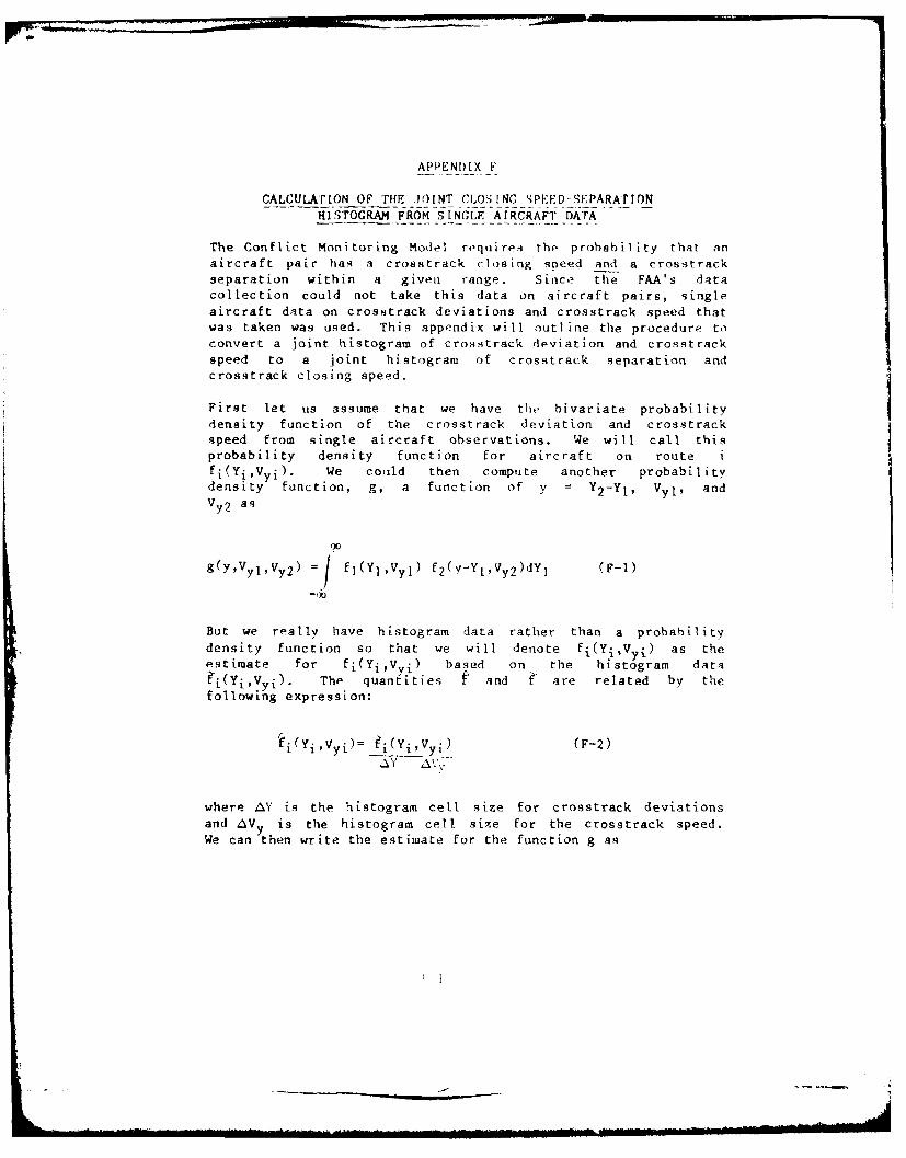
APPENDIX -F
CALCULATION OF TiE JOINT CLOSING SPEED-SEPARArIONHISTOGRA FROM SINGLE AIRCRAFT DATA
The Conflict Monitoring Model rquires the probability that an
aircraft pair has a crosstrack closing speed and a crosstrackseparation within a given range. Since the FAA's data
collection could not take this data on aircraft pairs, single
aircraft data on crosstrack deviations and crosstrack speed thatwas taken was used. This appendix will outline the procedure to
convert a joint histogram of crosstrack deviation and crosstrack
speed to a joint histogram of crosstrack separation and
crosstrack closing speed.
First let us assume that we have the bivariate probability
density function of the crosstrack deviation and crosstrackspeed from single aircraft observations. We will call thisprobability density function for aircraft on route i
fi(YiVi). We could then compute another probabilitydensity function, g, a function of y = Y2 -YI, Vyl, and
Vy 2 as
g(yVylvy2) =1 fl(Y]3 Vyl) f2 (y-YlVy2 )dY] (F-1)
But we really have histogram data rather than a probability
density function so that we will denote fi(Yi V -) as theestimate for fi(Yi,V) based on the histogram data
Si(YiVyi). The quantities f and f are related by the
following expression:
ii(YiVyi) = i(YiVyi) (F-2)
AY \v;
where AY is the histogram cell size for crosstrack deviations
and aVy is the histogram cell size for the crosstrack speed.
We can then write the estimate for the function g as

(y iV, 'y2) = ? V v) f, ~- AV o)
Y.- Y I AY
Y -cio y
11
y, -y AY(AX)
But
gY y I y g2 (y, V, IV, 2) -AY (zlV (F-4)
Therefore
The expression in (F-5) is the histogram convolution of thecrosstrack deviations. The result, g, is a histogram in termsof the spacing between the aircraft and their individualcrosstrack velocities. By letting ~V y2-' we canchange the variables in the function g. Thus-
g(yvyl,vy2) =g(V,Vy 2 - 9vy2)(-)
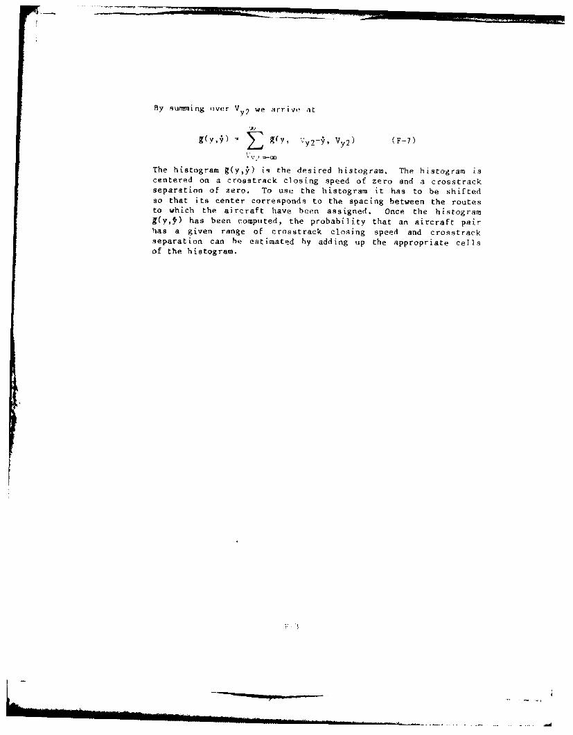
By gumming over Vy 2 we arrive at
(YY) (Y, '-y2- , Vy 2 ) (F-7)
The histogram g(y, ) is the desired histogram. The histogram iscentered on a crosstrack closing speed of zero and a crosstrackseparation of zero. To use the histogram it has to be shiftedso that its center corresponds to the spacing between the routesto which the aircraft have been assigned. Once the histogramg(y,v) has been computed, the probability that an aircraft pairhas a given range of crosstrack closing speed and crosstrackseparation can he estimated by adding up the appropriate cellsof the histogram.
:II

I-NTERVIE.NT ION RAI S. IM ULATI 0 N
G1. INTRODUCTrION
This appendix willI d i s(055 tho est imat ion of the controll >rintervention rate. The(- e-;t imate, o f this system pe r forma nce,measuire was obtained through a nimulation. The input data tothe simurlati~on will be titturihod fol Ilwod hv -ii outline of tMesteps the simulation performs,;( arr ive at the intervention raltestimate,;. The analysis ot the output from the simulat ionden I t wi th a t the end ()f t he aIppe-nd i x.
G2. THE INPUT
The data which were urs,,d in the simulation were smootha.a irc ra ft t racks wh ich a re pa rt: o f t he FAA's VOR nav iga t ion (!a t,Collection. Ahout lO aircraft on each of two selected ron! sin the Cleveland ARTCC were raindomly chosen over thle t ime p-c ioof the data collection. The only requirement on these aircraftwere that they had actual ly f'own the ent ire route segments ofinterest. The other data ust-i in the simulation are shown inFigure G- 1. These datiu incud, the radar noise and the locat ioof the radar, the route coor, 'na tes, the sec tor boundaries, *random number seed, the number Otf route spacings a &rpplic!at ions for the s imul ition to consider, and the rpquvstct
flow rates of the t ra ffic on t he routes. The time durat ionthe s imu1a, ion i s alIso spot ftid
G3. THE SIMULATION FLOW
The ohec t o f t he i mu I i ,i ; to est inmat 'he C'or Ir
intervention ra t , a t ;i,v-': W route spacings for severni t lowrates alIon g the rou t P g S ince t h is s a s imulIat ion1itexper imen t, " s ev- ra I re p I i ca-It i on s shIIot i b )e ma de s t than
meani ngfu 9 tatements an he made concrnig the results.
To minimize t he c os t of (hose ntrmeus ru n S, a defi ni t esimulation rtmn st ra tpgv wa K emp loved. The strategy depends, onlthe use of the same t raft ic for e achi diffe rent rooute spac ingduring t he same replication of the simulation. The minimumroute separat ion to be considered (S nimi )was i-un first. Of thetraffic run on the rout's spaced a minimurm distance apart, onlya subset of the traffic won u d form the set of potent ial1conflicts f or the next soet of Wider spaced routes. In ,therwords, with the same traffic, aircraft which are not projectedto get near to other aircrat at the narrower route spacing will

CONFLICT MO0NITORING ANALYSIS OF PARALLEL ROUTE SPACING IN THE 4 -ETC(U)JUL 80 A P SMITH DOT-FABOWA-4370
UNCLASSIFIEDi MTR79WO0235V0L2 FAA-EM-80-16 VOL 2 NL
7 A-AD412 MITEflf MLAN flflflflflIVFlflfl2

,. *32 22l
1.8
111111.25 1111.4 , I 1.6
MICROCOPY RESOLUTION TEST CHARTNATIONAL BUREAU OF STANDARDS-1963-A

TRACK fTH Ro-1 7~1F RANDOM NUMBEH F~LOW RATI',jI & I l ii NMBER ROUTE SPACINGI
IAT RADARATI[N
L READ IN AND ------
IRFI ( PTN IACOFL I T
I ADD RADARNOIS
TRACK AND PERFORM POTENT IAL-- - - - CONFLC T ALERT CONFLICTS
MORE
7PACrF. CARA(TFRI'.TIC',SAIG
rLe ING HOUR, !
CONFLICT ALERTSMAX [ACO)THER STATS
FIGURE G-1INTERVENTION RATE SIMULATION FLOW

not be projected to get near to other aircraft when the routesare farther apart. Of course some care must be taken inchoosing the definition of what it means to be projected to getnear to another aircraft for the purposes of carrying theaircraft along to the next route spacing. The reason for thiscare is that an aircraft pair may barely not be detected inconflict at one route spacing but might be detected in conflictat a wider route spacing. For instance, at the narrow routespacing, a deviating aircraft might be projected to pass infront of an aircraft on the adjacent route but with enoughseparation not to cause an alarm. However, with the aircraft inexactly the same positions except on routes that are spacedfarther apart, the projected minimum separation might be smallenough to trigger an alarm. To guard against not including suchaircraft in the wider route spacing sample an additional"window" which is larger than the conflict alert criteria wasemployed.
The flow of the simulation itself is rather straightforward asshown in Figure G-1. First, the traffic is generated. This isdone by randomly selecting a track from the track data. Thisdata consists of the best estimate of an aircraft's positionevery 12 seconds during the time the aircraft was observed inthe FAA's data collection. Next an entry time is chosen forthat aircraft. The entry time is chosen such that theinteraircraft entry t imea are exponentially distributedcorresponding to the desited average flow rate on the route.Since exponentially distributed interaircraft entry times couldallow two aircraft to be very closely separated in time alongthe same route, a check is made to insure that the radarseparation is not violated between aircraft on the same route.If an aircraft pair is detected to violate the separationstandard, the second aircraft is delayed at the route entrypoint to insure the minimum separation, plus a buffer, betweenthe two aircraft.
After the traffic is generated, the coordinates of the aircraftposition. are transformed to correspond to two routes that arespaced at the minimum spacing. At this point the simulation hasa string of positions and times that is organized by aircraft.To simulate radar returns, the aircraft positions must beorganized by time. This is achieved by sorting the aircraftposition records by time (radar update).
The simulation can now track and perform conflict alert on theaircraft positions. But before the simulation can performeither of these functions on a particular set of aircraft,
G-3

certain conditions must prevail. The first condition is thatthe time of the radar update must be between the starting andending time values of the simulation. These values are set whenthe traffic is generated to account for the "end effects" of thesimulation. The simulation does not start until the latter ofthe first aircraft on each route exits the sector. Thesimulation ends when the earlier of the last aircraft on eachroute enters the sector. After the starting update, the trackerwill maintain a track on all the aircraft.
The positions of the aircraft from the "track data" have beensmoothed as part of the FAA's dita collection program.Therefore, radar noise (azimuth and tange) is added to theposition reports prior to going into the NAS tracker in thesimulation. The tracked aircraft are then subjected to theconflict alert function if two further conditions are met. Onecondition is that both aircraft have to be within the sector ofinterest. The other condition is that there has not been aprevious conflict alert declared on this aircraft pair.
An aircraft pair which satisfies the above conditions are thenpassed to the conflict alert function where the pair issubjected to a set of coarse geographic and velocity filters.Passing these coarse filters indicates that the pair is near andgenerally closing on each other. The aircraft pairs that passthe coarse filtering are then subjected to a set of finefilters. These fine filters project the positions of the pairahead in time. If, within a given look-ahead time, the pair isprojected to be separated by less than a certain distance, thenthe pair is called a conflict pair. If the pair passes the finefiltering in two out of the last three passes through thefilters then the pair is in potential conflict. In the WAS, thecontroller is alerted to this conflict pair by the WASautomation blinking the aircraft symbology on his screen. inthe simulation, the potential conflict is tallied as part of thesimulation statistics. The current conflict and predictedconflict parameters are the same ones used in NAS. In additionother parameters are used by the simulation to identify thoseaircraft pairs which should be included in the next wider routespacing run. The definitive formulation of the RAS ConflictAlert function can be found in Reference (13). Appendix H givesa detailed description of the horizontal components of the WASConflict Alert.
Referring back to Figure G-1, ye can see that after the conflictalert has been performed, we have a list of nearly conflictingpairs of aircraft to be used in the simulation of the next wider
G-4

route spacing. If there are no mtore nearly coniflicting pafra orthere are no more route spacings to consider, we go back to doanother replication of the simulation. If there are nearlyconflicting pairs and more route spacings then the simulationreassigns, the nearly conflicting pairs to the routes. The sameentry times that they had originally are maintained. The newlyassigned aircraft's positions are then transformed to correspondto the new route spacing. The loop is thus closed and theprocessing continues until all the route spacings andreplications are done.
G4.. THE OUTPUT
The output from the simulation consists of several statistics.First, the traffic generator lists the traffic characteristics:the particular aircraft chosen, their entry times onto theroutes, the delays that were incurred, and the realized averagetraffic flow rates. The tracking and conflict alert part of thesimulation records another set of statistics. These includethe number of flying hours in the sector, the number of aircraftgenerating those flying hours, the maximum instantaneousaircraft count (IAC), the number of hours the conflict alertfunction was "watching" the sector, and the number of conflictalerts declared. Other miscellaneous statistics concerning thedetailed workings of ccnflict alert are also zaken.
G5. THE AIIAYSIS OF THE OUTPUT
As Reference (14) points out, there are basically two types ofsimulations as far as the analysis of the simulation output isconcerned -- terminating and steady-state. The differencebetween these is the desired result. in all cases a simulationhas to be terminated after some finite time interval. In somecases, one wishes to evaluate steady state property of thesystem as if the time interval goes to an infinite length. Inother cases, the behavior of the system over a defined(terminated) length of time is desired such as the peak of thetraffic demand. The simulation of conflict alerts belongs tothe terminating type of simulation. one of the results ofReference (14) is that for a terminating simulation the usualstatistical tests and procedures can be applied to the outputfrom the simulation.
In the particular simulation described above, the event of aconflict alert occurs over a period of time. It is also aslikely that this event will occur in one interval as in anyother and that the occurrence of the event has no effect on
G9

j
whether or not another occurs. The number of events in a f ixedtime with the above attributes is often assumed to have aPoisson distribution. In fact in the results section (Section 5in Volume I of this report) it is shown that the number ofconflict alerts per hour from the simulation does look as if itwere Poisson distributed.
The result ye are looking for is the expected value of thePoisson distribution. The unbiased and maximums likelihoodestimator is the sample mean. This is the number of conflictalerts divided by the number of hours which were simulated. Wecan also construct a confidence interval for the expected valueof a Poisson distribution (Reference (15). If
f(n) n - 0,1,2...(G)
then for any value n' and &<.S, lower and upper limits of maybe determined such that
n-nn
and (G-2)
no eA ba
such that X < )b The values of X. and Xb are tabulatedfor 100(1-2&1% - 952 and 992 significance levels in Reference(15). These tables are applied to the simulation output toconstruct 952 confidence intervals for the expected rate ofconflict alerts. The results are shown in Section 5 of Volume Iof this report.
G- 6

1|
APPENDIX K
THE NAS CONFLICT ALERT
In Section 3.1.1 of Volume I of this report it was stated thatthe conflict alert function in the NAS computer was not modelledprecisely in the Conflict Monitoring Analysis. The NAS ConflictAlert function uses both horizontal and vertical filters whendetermining the condition of conflict between a pair ofaircraft. Since we have assumed the aircraft to be in straightand level flight at the same altitude, this appendix will
discuss only the horizontal filters used by the NAS ConflictAlert function.
In the NAS computer the Conflict Alert performs a series of
tests to determine the conflict status of a pair of aircraft.The tests are structired in such a way as to minimize falsealarms, maximize the chance of an alarm on a true conflict whileat the same time minimizing the computational complexity of thetests.
After the tracks are geographically sorted and tested for beingnear in altitude, a series of horizontal filters are applied.The filters are diagranmed in Figure H-1. The Conflict Alerthas two types of horil.ontal filters, coarse and fine. For eachtype there may be two levels designated as A and B. The typeand level of the filter will depend on the previous history ofthe aircraft pair with respect to the Conflict Alert function.The values of the Conflict Alert parameters are summarized onTable H-1.
The process starts with position estimates (X, X"J Y ,
Y) and velocity component estimates O, Xj, Yi, YQo! aircraft i and j. It is first determined what type and levelof filter should be used. The choice will depend on whether theaircraft pair has been observed previously and, if so, what theresult of the previous Conflict Alert tests were. If theaircraft pair has not passed any filters successfully in thepast two applications of the filters, a level A filter is used.If a level A filter is required then a coarse horizontal filteris performed on the position estimates:
(Xi-Xj)2 + (Yi-Yj)2 - MAXR2 (H-1)
where KAXR-55 nmi. If the aircraft are separated by more than55 nmi they are no longer considered by Conflict Alert.
11- 1 I

3cc
U.
z
H-2

a~
-D -- a c
E E~E..- 4IIs
0e 0 OrO. 0 00
U') Ln O c0 %D Cjo .
m 04 ES- E-4*
0u
or a-' L) V w- U ,E-M- -t w - P1cr i-
0 tn u V; r. t") EcN
H H--
P-4 0. H H
0 CCL4 u u
E- V) F:-
Ca. u1
0U C&.

If the coarse filter is passed the positions and velocities ofthe aircraft pair are subjected to the fine filter of level A.
The fine filter first checks if the aircraft pair is in currentlateral conflict. If
R - (Xi-Xj)2 + (yi-yj) 2 (H-2)
is less than SEPR 2 , a current horizontal conflict exists. For
level A SEPR - 5 nmi and for level B SEPR = 4.2 nmi.
If the aircraft pair is not in current conflict, it could be inpredicted conflict. This part of the fine filter projects anaircraft pair ahead in a straight line for a certain period intime and tests to see if the aircraft come within a givendistance of each other' during that time interval. This check isdone in several steps to reduce computation time. The firststep is to determine whether the tracks are generally converging
toward each other. If we let
Vc=(Xi-xj)(ii-1j)+(Yi-Yj)(ii-tj) (]3
then the inquality Vc < VELC must be satisfied to continuetesting. For both level A and level B, VELC-8 nmi2 /hr. Thesign of quantity Vc indicates a closing condition in the Xand Y directions. If the aircraft were closing in both X and Ysimultaneously then /c would be less than zero. If theaircraft were opening in both X and Y simultaneously, then Vcwould be positive. If the aircraft were closing in onedirection and opening in the other direction, the value of Vc
may be positive or negative. Even if Vc is positive the missdistance might be small enough to qualify as a potentialconflict. Thus Vc is tested against a positive number.
If the aircraft are closing, they may be doing so very slowly.If the closure is too slow there cannot be a conflict within theprescribed time interval. If we let
V2-(Ii-ij)2 + (ti-tj) 2 (H-4)
then the inquality V2 >CLOS2 must be satisfied to continuetesting. CLOS is equal to .7 nmi/min for both level A and levelB.
The predicted minimum separation is tested next. The time tominimum separation, Tm, is -Vc/V2 . If V2 0, thenTm=O. The square of the predicted minimum separation is
= - * (H-5)
H-4

If R4 -SEPM 2 then the checking can continue. For level A
SEPH is set to 6 nmi. For level B SEPM is set to 4.8 nmi. The
window is opened wider on level A to allow for a turning
aircraft to be detected at the earliest moment.
After it is determined that the aircraft are predicted to close
to less than the preset minimum, a test is performed to
determine if the minimum separation is violated within the
look-ahead time (WRNT). For level A WRNT - 2.5 min. For level
B, WRNT - 2.0 min. The minimum separation is violated within
the look-ahead time if one of the following conditions holds:
& The time to minimum separation, T., is:less-'than orequal to WRNT or
* The square of the separation predicted at WRNT violates
the separation limits.
The square of the separation predicted at WRNT is given by
R2(WRNT)=R2+(2Vc*WRNT)+V2*WRNT2 (H6)
Violation of the separation limits occurs when
R2(WRNT)Y SEPP 2 .
The value of SEPP for level A is 6 nmi. For level B the value
is 4.8 nmi. Here again, the longer time window on level A isdesigned to allow more efficient detection of accelerating
aircraft.
If an aircraft pair passes both the fine horizontal filter and
the fine altitude filter (which is not being considered here) at
level A then it is placed in a conflict pairs table. On the
next tracking cycle this conflict pair will be tested against
the level B set of filters. An aircraft pair is eligible for
controller alert generation if it has been determined to be in a
condition of conflict at least twice in the past three sucessive
applications of the filters. This procedure reduces the rate of
false alarms due to noise in the surveillance system. Once an
aircraft pair has been in a condition of conflict for the
requisite number of successful tests, the pair will be
identified to the controller by flashing data blocks and list
displays at the controller's position. This flashing will
continue as long as the aircraft pair continues to meet the
Conflict Alert criteria or the controller manually turns off thealarm.
11-5
L- r | II
n 'i-zn.

The parameters in Table H-1 labeled as Near Conflict parametersare those used by the interviention rate simulation described inAppendix G. These parAMet.ors are used to identify thos~e pairsof aircraft that miglit he' potential conflict pairs in thesimulation run at a wider rouste spacing.
H1-6

APPENDIX I
CLOSSARY
A The total Ielay time at which the aircraft
pair will come into horizontal overlap
before there is an avoidance turn. (Figure
3-5, Volume I).
A' One corner of the polygon B (Figure C-4,
Volume IT).
A,, A2 The alongtrack positions of two aircraft on
their respective routes (Figure E-1, Volume
IT).
ACP Azimuth Count Pulse. A unit of angular
measure equal to 1/4096 of a circle (.0979degrees) (Table 5-1, Volume T).
a A parampter of the integral of the circular
normal probability function (Equation C-6,
Volume TI).
B The polygonal area over whicch one computes
the probability of observing an aircraft
pair (Figure C-4, Volume TI).
B' One corner of the polygon B (Figure C-4,
Volume TT).
B1 The alongtrack position of an aircraft on a
route (Figure E-1, Volume IT).
b The starting time of the periodic
observations (Section D-4, Volume i).
A parameter used to fit the envelope for the
horizontal overlap region (Equation B-21,Volume TI)
CLOS Closing Speed Threshold parameter (EquationH-4, Volume II).
C' One corner of the polygon B (Figure C-4,
Volume II).
T-1
iji i_....1

D The minimum projected separation between an
aircraft pair used by the conflict alertfunction (Equation 3-4, Volume I).
D' One corner of the polygon B (Figure C-4,Volume IT).
d The separation between two aircraft
(Equation A-I, Volume II).
DMIN The minimum separation between a pair ofaircraft (Figure 3-3, Volume I).
E(W) The expected value of the separation betweenaircraft on the same route (Equation E-3,Volume IT).
F The crosstrack distance inside the conflictregion at the initial radar observation(Figure B-2, Volume IT). The partitioningparameter for the crosstrack closing speed
(Equation R-18, Volume II).
FFT The Fast Fourier Transform (Appendix D,Volume IT).
f(n) The Poisson probability density function
(Equation G-l, Volume IT).
F(n) A finite Fourier transform (Equation (D-l),Volume IT.
f(t) A finite, complex series (Equation D-1,Volume I[).
f(W) The probability density function of the
separation between two aircraft on the sameroute (Equation E-1, Volume I).
F(Yi,Vyi) The histogram data corresponding to f.
(Equation F-2, Volume Ii).
Fe(n) The even elements of the transformed series,F(n) (Equation D-6, Volume I).
fe(t) The even elements of the series f(t)(Equation D-6, Volume I).
1-2

fi(YitVyi ) The joint probability density function ofcrosstrack deviation and crosstrack speedfrom single aircraft observations fromaircraft on route i (Equation F-1, VolumeTT).
i(YiVyi) The estimate for fi(YiVyi) (EquationF-2, Volume IT).
fi(YiVyi) The histogram data associated with theprobability density functionfi(Yi,Vyi) (Equation F-2, Volume IT).
Fo(n) The odd elements of the transformed series,F(n) (Equation D-6, Volume I).
fo(t) The odd elements of the series f(t)(Equation D-6, Volume If).
G The crosstrack separation lost during oneradar update time interval (Figure B-2,Volume I).
The gravitational constant (Equation B-6,Volume IT).
G(n) A finite Fourier Transfirm (Equation D-5,Volume 1I).
g(t) A finite, complex series (Equation D-5,Volume I1).
The derived histogram of crosstrackseparation and crosstrack closing speed.(Equation F-7, Volume II).
g(yVylVy2) The joint probability density function ofthe crosstrack separation and the twocrosstrack speeds (Equation F-1, Volume IT).
g(yVylVy2) The estimate for g(yVylVy2) (EquationF-3, Volume IT).
g(yVyl,Vy2) The histogram data corresponding to(Equation F-4, Volume IT).
H Dummy Variable (Equation B-14, Volume II).
1-3
It

h A distance defined in Figure C-6, Volume It
h(t) The convolved density function (EquationD-11, Volume i).
h(,) The probability density function of the bankangle K (Figure B-4, Volume II).
h(x) The probability density function of thealongtrack distance between aircraft on oneroute and an aircraft on an adjacent route
(Equation E-2, Volume 1I).
T Dummy Variable (Equation B-14, Volume IT).
TAC Instantaneous aircraft count (Appendix G,Volume 11).
J Dummy Variable (Equation B-14, Volume IT).
j(w) The probability density function of the turnrate w(Equation B-1, Volume II).
K Durmy Variable (Equation B-14, Volume IT).
kl,k 2 Distances defined in Figure C-6, Volume IT.
L Dummy Variable (Equation B-14, Volume 11).
M Dummy Variable (Equation TI-14, Volume Ii),(Appendix A, Volume IT).
MAXR The maximum separation at which ConflictAlert will continue to consider a pair ofaircraft (Equation H-1, Volume IT).
N The half series length (Equation D-6, VolumeII), also the number of equally spacedinitial positions in the Conflict RegionBoundary (Equation B-5, Volume I).
n Index of the FFT (Equation D-l, Volume I).
N1,N 2 The average flow rate of aircraft on routes1 and 2 (Equation 3-7, Volume I).
P The factor which delineates the three casesof overlap (Equation B-11, Volume I).
T-4

PFD i The probability of first detecting anaircraft pair on update i. (Equation B-4,Volume IT).
PFDi, F The probability of first detecting anaircraft pair on update i given the first
observation was at F. (Equation B-2, Volume
IT).
PH The proportion of time that the horizontalseparation is lost (Section 2.2, Volume I).
Pki The probability that the time delay has avalue in the kth cell. This probabilitywill also depend on the conflict region
boundary cell, i. (Equation B-27, Volume II).
Pe The probability that the turn rate has avalue in the ith cell (Equation B-27, VolumeII).
PNDiF The probability that the aircraft pair willnot be detected in the conflict region onradar update i given the first observationwas at F (Equation B-J, Volume Ii).
pNDi,F The probability of not being detected in the
conflict region during the first i updatesgiven the first observation was at F.
(Equation B-1, Volume II).
Px The proportion of time that the alongtrack
separation is lost (Section 2.1, Volume I).
P y The proportion of time that the crosstrackseparation is lost (Section 2.1, Volume I).
P(CB) The probability of an aircraft pair being onthe conflict region boundary (Equation B-23,
Volume IT).
P(CBi ) The probability of an aircraft pair being on
the conflict region boundary in integrationcell i. (Equation 3-2, Volume I).
P(HOICB i ) The probability of an aircraft pair cominginto horizontal overlap given that the pairstarted on the conflict region boundary in
integration cell i (Equation 3-2, Volume I).
T-5

P)()Fi I Yl ,Yi 940 The join) probability that the aircrafr pairhas a crosstrack separation yi in the ithcell and has a crosstrack closing speed yiin the ith cell (Equation B-26, Volume 1I1.
P. The probability that an aircraft pair has aninterroute alongtrack separation a x(Equation 3-4, Volume I).
Qn The number of multiplications required forcalculating the transform of air N pointarray. (Equation D-7, Volume IT).
q(F) The probability density function of thedistance inside the conflict region boundary
at which the first observation is made
(Equation B-3, Volume IT).
R The radius of the right cylindricalcollision shape (Section 3.2, Volume T).
Rm The predicted minimum Separation (EquationH-5, Volume Ii).
Ro The lateral separation between tracks(Equation H-2, Volume II).
Rp Predicted separation at the warning time(Equation 11-6, Volume IT).
rk~i The proportion of the k th cell in theoverlap space is enclosed within thehorizontal overlap region corresponding to
the ith conflict region boundary cell(Equation B-27, Volume IT).
9EPM Minimum Separation Parameter (Equation H-5,Volume IT).
SEPP The separation at the warning time parameter(Equation H-6, Volume I).
SEPR The current lateral conflict threshold(Equation H-2, Volume II).
T The number of elements in the series onwhich the FFT operates (Equation D-l, Volume
-).
1-6
. ... . . . . . - . . .

The rime variable, also n .4immation index
td The total delay time, from the time theaircraft pair enters rhe conflict region tothe time one aircraft stArts its avoidancemaneuver. (Equation B-10, Volume IT).
TL The look-ahead time in the conflict alertfunction (Equation A-3, Volume IT).
To Time to minimum separation (Equation H-5,Volume II).
t t The time the aircraft is in the turn to thepoint of closest approach (Equation B-10,Volume IT).
Ti1 The time the aircraft pair is at theconflict region boundary (Figure 3-3, VolumeI).
T"2 The time at which the system has cognizancethat the aircraft pair is within theconflict region (Figure 3-3, Volume I).
T 3 The time at which the aircraft start itsavoidance maneuver (Figure 3-3, Volume I).
u A coordinate axis used to circularize thebivariate normal distribution (Equation C-3,Volume IT).
'Jl The u coordinate value of point A' (EquationC-9, Volume IT).
u? The u coordinate value of point B' (EquationC-9, Volume IT).
V The forward velocity of the aircraft
(Equation 3-7, Volume 1).
v A coordinate axis used to circularize the
bivariate normal distribution (Equation C-3,Volume TI).
Vc Converging speed indicator (Equation H-3,Volume I).
VELC Converging speed threshold parameter
(Equation H-3, Volume I).
T-7
_ _ 7

V2 Closing speed indicator (Equation 11-4,Volume I).
Vxn The tracker x velocity estimate for 4can i
(Equation C-1, Volume TT).
Vxl,Vx2 The alongtrack speeds of aircraft on routesI and 2 (Figure A-I, Volume II).
Vymax The maximum croastrack speed observed in thedata (Equation A-4, Volume II).
Vvn The tracker Y velocity estimate for scan n
(Equation C-i, Volume II).
Vyl,Vy2 The crosstrack speeds of aircraft on routesI and 2 (Figure A-i, Volume II).
V(h,k) The integral of the circular normalprobability function (Equation C-6, Volume1i).
V i The v coordinate value of point A' (EquationC-9, Volume IT).
v2 The v coordinate value of point R' (EquationC-9, Volume Ii).
W The separation between two aircraft on the
same route (Figure E-1, Volume IT).
WRNT Warning Time (Look-ahead time) (Equation
H-6, Volume II).
x The alongtrack, interroute, separation
between a pair of aircraft (Section 3.2,Volume I).
The alongtrack, interroute, closing speed
between a pair of aircraft (Equation A-l,Volume TI).
A1,*2 The bounds on the value i (Equation A-7,Volume TI).
Xi The alongtrack position of an aircraft on
route i (Figure A-I, Volume IT).
T-8
.. .__. .. .. .. . . . . . . . .

ii The alongtrack component speed of anaircraft on route i (Equation H-3, VolumeI).
Xi(t) The alongtrack tragectory of the aircraft onroute i (Equation B-9, Volume Ii).
xi The alongtrack, interroute, separation of anaircraft pair in the ith integration cell(Figure 3-4, Volume I).
Xpn The tracker predicted X position estimatemade at scan n for the position at scan n+l(Equation C-i, Volube II).
XtM The reported X position to the tracker fromthe surveillance ststem t scan n (EquationC-1, Volume 1I).
Ion The tracker X position estimate for scan n(Equation C-1, Volume Ii).
Xio Yio The X and Y positions of an aircraft onroute i when it is on the conflict region
boundary in conjunction with anotheraircraft on the other route. (Equation B-9,Volume II).
x(t) A series of data points (Equation D-8,Volume II).
Y The crosatrack separation between a pair ofaircraft (Section 3.2, Volume I).
The croastrack closing speed between a pairof aircraft (Section 3.2, Volume I).
Ti The crosstrack deviation of an aircraft fromthe centerline of route i (Figure A-1,Volume II). Also the Y component(crosstrack) position of an aircraft onroute i (Equation H-i, Volume I).
fi The crosstrack component speed of anaircraft on route i (Equation H-3, Volume
9).
I-9

Yi(t) The croastrack trajectory of the aircraft onroute i (Equation B-9, Volume II).
Yi The croastrack separation of an aircraftpair in the ith integration cell (Figure3-4, Volume I).
i The crosstrack closing speed of an aircraftpair in the ith integration cell (Figure3-4, Volume I).
¥i,F The croastrack separation at radar update iafter crossing into conflict region andbeing initially observed at F (Figure B-2,Volume II).
Tpn The tracker predicted Y position estimatemade t scan n for the position at scan n+l(Equation C-l, Volume II).
Yrn The reported Y positi6n to the tracker fromthe surveillance system at scan n (EquationC-l, Volume Ii).
Yon The tracker Y position estimate from scan n(Equation C-1, Volume II).
Yo The crosstrack separation at the conflictregion boundary (Figure B-2, Volume II).
y(t) A shifted series of data points (EquationD-8, Volume I).
z A variable which is minimized and maximizedin Appendix A. (Equation A-6, Volume II).
z(t) The convolved density function (EquationD-ll, Volume II).
o The NAB tracker position gain (Equation C-1,Volume I), and the significance level forhe confidence interval of the expected value
of he Poisson distribution (Equation G-2,Volume I).
The NAS tracker velocity gain (Equation C-l,Volume II).
A A fixed sampling interval (Section D-4,Volume II).
1-10

4Vy 11Th ibtorram cell sizo for crosstrack speed(Equation F-?, Volume If).
4X "The integration interval in the mlongtrackdimension (Figure 3-4, Volume I).
The integration inverval in the crosstrackdimension (Figure 3-4, Volume I).
The integration interval in the crosstrackclosing speed dimension (Figure 3-4, VolumeT).
lay The histogram cell size for crosstrackdeviations (Equation F-2, Volume IT).
KThe bank angle of the aircraft making theavoidance maneuver (Equation B-6, Volume 11).
The lower, KL, and upper, KU, hounds on thehank angle distribution (Equation B-7,
Volume TO).
A parameter of the integral of the circularnormal probability Function (Equation C-6,Volume TI), and the parameter of the Poissondistribution (Equation G-1, Volume II).
ka X) The lower and upper confidence limits on theexpected value of a Poisson distribution(Equation C-2, Volume I1).
The length of the rectangular collisionshape which represents the aircraft (Table5-1, Volume T).
X Y The width of the rectangular collision shapewhich represents the aircraft (Table 5-i, VolumeI).
The expected value of the crosstrack separationof an aircraft pair (Equation C-2, Volume 1I).
The expected value of the crosstrack closingspeed of an aircraft pair (Equation C-2, Volume
IT).
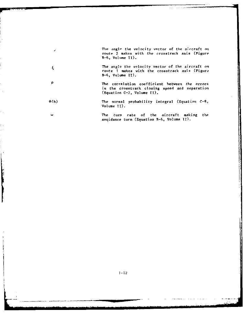
The angle the velocity vector of the aircraft onroute 2 makes with the crosatrack axis (FigureB-6, Volume IT).
The angle the velocity vector of the aircraft onroute I makes with the crosstrack axis (FigureB-6, Volume Ii).
P The correlation coefficient between the errors
in the crosstrack closing speed and separation(Equation C-2, Volume IT).
(h) The normal probability integral (Equation C-8,Volume IT).
The turn rate of the aircraft making the
avqidance turn (Equation B-6, Volume IT).
1-12
wn-

APPENDIX J
REFERENCES
1. Flener, Wiliam M., "Request for E&D Effort," Letter from the FAA
Associate Administrator for Air Traffic and Airway Facilities to the FAA
Associate Administrator for Engineering and Development, November 9,
1976.
2. Kirkendall, N.J., "A Specification for a Data Collection to
Determine Lateral Pathkeeping of Aircraft Flying VOR Defined Routes in
High Altitude En Route Areas," The MITRE Corporation, MTR-7430,Washington, D.C., June 1977.
3. Kirkendall, N.J., and Smith, A.P., "An Extension to the Data
Specification for the High Altitude Lateral Pathkeeping Study," The
MITRE Corporation, MTR-7638, Washington, D.C., December 1977.
4. Colamosca, B.F., Arch, H.L., Parkins, K.D., "Data Collection for
Study of Lateral Separation of Aircraft Flying CONUS High Altitude
VOR-Defined Air Routes," NAFEC Technical Letter Report NA-78-24-LR,
RTCA Paper No. 69-78/SSRG-18, May 1978.
5. Busch, A.C. and Colamosca, B.F., "Modeling Safety in a Procedural
Air Traffic Control Environment," Draft NAFEC Letter Report
NA-77-57-LR, RTCA Paper No. 155-77/SSRG-1l, October 1977.
6. Polhemus, N.W., "Introduction to a General Collision Risk Model for
Intersecting and Nonparallel Routes," RTCA Paper No. 9-79/SSRG-27,
January 1979.
7. George, P.H., Johnson, A.E., and Hopkin, V.D., "Radar Monitorng of
Parallel Tracks -- Automatic Warning to Controllers of Track Deviations
in a Parallel Track System," Eurocontrol Experimental Center Report
No.67 (Task C21/1), September 1973.
8. Johnson, N.L., and Kotz, S., "Distributions in Statistics:
Continuous Multivariate Distributions," New York: John Wiley & Sons,
Inc., 1972.
9. IEEE Transactions on Audio and Electroacoustics, Vol. AU-15, No. 2.,
June 1967.
10. Kleinrock, L., "Queueing Systems, Volume 1: Theory," New York: John
Wiley & Sons, Inc., 1976.
J-1
1!

11. "Methodology for the Derivation of Separat'on Minima Applied to
the Spacing Between Parallel Tracks in ATS Route Structures," ICAO
Circular 120-AN/89/2, 1976.
12. Kirkendall, N.J., "Probability of Passings Between Aircraft on
Adjacent Parallel Routes: Observed Data vs Model Estimates," The
MITRE Corporation, WP-79W00397 Washington, D.C., June 1979.
13. Hauser, S.J., Dodge, P.O. and Steinbacher, J.G., "Computer
Program Functional Specifications for Conflict Alert," The MITRE
Corporation, MTR-7311, Washington, D.C., September 1976.
14. Law, A.M., "Statistical Analysis of the Output Data from
Terminating Simulations," Unpublished and Undated Report supported
by the Office of Naval Research and the Army Research Office.
15. Handbook of Tables for Probability and Statistics. The Chemical
Rubber Co., Cleveland, Ohio, 1968.
J-2