7 AD-All 051 NAVAL POSTGRADUATE SCHOOL MONTEREY CA

F/ 5/1MODEL OF ORGANIZATIONAL DECISION PROCESSES.IW)

UNLSIIDMAR Al W Y KIMUNLASSIFIEE|E I

Eh||h|hEEE|w|

LEVEL

NAVAL POSTGRADUATE SCHOOLMonterey, California

B I

THESISA MODEL OF ORGANIZATIONAL DECISION PROCESSES

by

Woo Youl Kim

March 1981

Thesis Advisor: Dan C. Boger

Approved for public r3lease; distribution unlimited

j.

,,*,

UNCLASSIFIEDSECuRITY CLASsPirCAion OF TwIS PAGE r0to ole gond _________________

MZAD INSTRUC*TIfNSREPORT DOCMENTIOM PAGE 317033L COMPLE7TNG FORM1. REPORT NUMBER S. OVT ACCESU@N wo: S. RECIPIENT'S CATALOG M4US169

41. TITLE fallsed*hi.) S. TYRE OF REPORT 6 PERIOD Coveato

A Model of Organizational Decision master's Thesis;Processes March 1981

a. PERFORMING ONG. 11140111 PIMEERa

7. AUT1NOfa -S. ONTRACT OR GRAIOT Mum..NSR(o)

Woo Youl Kim

9. PERFORMING ORGANIZATION NAME AND ADDRESS I@. PROGRAM ELEMENT. PROJECT. TASKNaval Postgraduate School AREA 6 WORK UNIT NUNUERs

Monterey, California 93940

I I. coNTrROLLING OPPICE NAME AND ADDRESS 12. REPORT DATE

Naval Postgraduate School March 1981Monterey, California 93941 is. NMum"ErOPAGES

50 pages14. MONI1TORiNd AGENCY NANI & AOOWES8II 014ififtII.M C.,JPJMO Office) IS. SECURITY CLASS. rot rhi. eftmn)

Unclassified

1. OEC LASM F1 CATION/ DOWN6GRIAOINGSC NEDUL9

14. DISTRIBUTION STATEMENT (of Ws Ropme)

Approved for public release; distribution unlimited.

17. OISTRIOUTION STATEMENT rot the oabwrst antoued In WIok 20. it dEifwomf t RJpt)

IS. SUPPLEMENTARY NOTES

IS. K EV vORlos (Con.Uawe an mroroe soda i mwdIr ONe', end IRI r W beek Arnbm

PPBS, multiple period planning

20. ASETRACI (CaseINue -GOw. OIMP4oS It 00006"M Si IuSRID010 OF leed 0=nA6.)

..-he generalized goal decomposition model proposed by Ruefli as asingle period decision model is presented for the purpose of areview and extended to make a multiple period planning model. Themultiple period planning model in the three level organization isformulated with linear goal deviations by introducing the goalprogramming method. Dynamic formulation using the generalized goaldecomposition model for each single period problem is also pre-sented. An iterative search alaoritbxn is oresented as an

DO AN 43 EIINO NV6 sOSLT UNCLASSIFIED66CURIly CLASIFICATIOM OF TWIS PAGE rnfoczeIew hWe

UNCLASSIFIEDr.iIm'. CLAMP6 M%. ftfns e6'Ugo &ame.=llvw 09 Ime &a

appropriate solution method of the dynamic formulation of themultiple period planning model.

INSP( CTLL)

OD1 'orl 14T3 2 UNCLASSIFIEDS/4 61%3.014-6601 6OO MGOITINoTo$vsfb&wewb$sCevq'v gbMSISgAIU O9 fug00 .. mo~lla g gUe~mob~

• •. .. . . . .. . .. * .... *

Approved for public release; distribution unlimited

A MODEL OF ORGANIZATIONAL DECISION PROCESSES

by

Woo Youl KimLieutenant Colonel, Korean Army

B.S. Korean Military Academy, 1967

Submitted in partial fulfillment of therequirements for the degree of

MASTER OF SCIENCE IN OPERATIONS RESEARCH

from the

NAVAL POSTGRADUATE SCHOOLMarch 1981

Author:

Approved by: Id CThesis Advisor

v Second Reader

Chai rm111, Department of Operation9Research

Dean of Information and Policy Sciences

3

ABSTRACT

The generalized goal decomposition model proposed by

Ruef ii as a single period decision model is presented for

the purpose of a review and extended to make a multiple

period planning model. The multiple period planning model

in the three level organization is formulated with linear

goal deviations by introducing the goal programming method.

Dynamic formulation using the generalized goal decomposition

model for each single period problem is also presented. An

iterative search algorithm is presented as an appropriate

solution method of the dynamic formulation of the multiple

period planning model.

4

TABLE OF CONTENTS

I. INTRODUCTION-------------------------------------------- 6

II. GENERALIZED GOAL DECOMPOSITION MODEL-----------------9

III. MULTIPLE PERIOD PLANNING APPROACH OF THE GENERALIZED

GOAL DECOMPOSITION MODEL------------------------------ 18

A. LINEAR FORMULATION OF THE MULTIPLE PERIOD

PLANNING -MODEL------------------------------------- 19

B. DYNAMIC FORMULATION OF THE MULTIPLE PERIOD

PLANNING MODEL------------------------------------- 26

C. SOLUTION METHOD OF THE MULTIPLE PERIOD PLANNING

MODEL---------------------------------------------- 3

IV. SUMMRmY------------------------------------------------- 4

LIST OF REFERENCES------------------------------------------- 49

INITIAL DISTRIBUTION LIST------------------------------------ 50

I. INTRODUCTION

Major issues relating to the choice of resource alloca-

tion mechanisms appear in the decision making process because

of the huge size and complexity of most organizations. De-

centralization will be or should be undertaken due to condi-

tions of uncertainty and lack of information. An organization

is rarely presented with a clear-cut objective function.

It's objective functions do not remain constant but grow out

of its experiences and out of the changing external environ-

ment. If everything were known and certain and unchanging,

the total problem could be solved without compartmentaliza-

tion. In fact, in an unchanging world, decision making

itself would become trivial. The problems could either be

solved by the central unit or passed down to subordinate

units with explicit instructions which would insure that

the solution be the same as that obtained by the central

unit. However, the objective functions do not remain fixed.

According to Smithies, decentralization involves some

degree of delegation of decision making authority. It can

arise from the deliberate intent of the central authority

or from centrifugal forces within the organization where

complete centralization is unfeasible or undesirable. De-

centralization almost inevitably involves some conflict of

point of view between the central authority and lower

6

decision making levels. The conflict, however, may lead to

better results than that occurring in apparently clear-cut

centralized processes.

In the real world, it is necessary to divide the problems

into components that are meaningful according to relevant

criteria. The optimizatioi. dhich includes the use of de-

centralization may continue to be utilized with the recogni-

tion that lack of information and uncertainty are inherent in

the system. Stated in other words, the decision maker may

approach a given problem more effectively in terms of sub-

problems due to lack of information about objective costs

and technology. From the knowledge that is gained by dealing

with the subproblems, the decision ma~ker gradually builds up

a solution.

Ruefli has proposed the generalized goal decomposition

model with a three level organization as a single period

model. The organization consists of a central unit, manage-

ment units and operating units. Each level is vertically

interrelated by a specific information flow. Levels of

organization are assumed to be horizontally independent.

The central unit coordinates the activities of the M manage-

ment units by selecting goals and resource levels for these

units. The management units choose activity levels for

various projects in an attempt to meet the goals and resource

levels set by the centra. -unit. The operating units are re-

sponsible for generating project proposals for their respec-

tive management units.

7

It

In fact, most of the organizations are concerned with a

planning horizon that is more than a single period in length.

If the planning horizon is restricted to a single period,

then it is actually difficult to make an appropriate evalua-

tion of the alternatives because there can be a lack of

relationships and information between planning periods and

between levels of the organization.

In this paper, the generalized goal decomposition model

is extended to the multiple period planning model of an

organization in order to get more realistic alternatives

into the decision making process.

8

II. GENERALIZED GOAL DECOMPOSITION MODEL

The generalized goal decomposition model proposed by

Ruefli is a goal programming model of an organization where

the solutions depend upon the structure of the organization.

His model is structure dependent and goal oriented. The most

unique feature of the generalized goal decomposition model

is that it is difficult to speak of its possessing a global

objective function. Upon reflection on the nature of

organizations, this is natural since the model is, for the

most part, motivated by the problem of decomposing one large

problem into its component parts.

Ruefli formulates the problem for the whole organization

in terms of the problems of the organizational subunits and

does so in such a manner that it is impossible to speak of

the global objective except in terms of the objectives of

the organizational subunits. This is primarily because goal

programming deals with vector optiizations.

The model involves a three level organization. The

central unit represents the top level of the organization

is responsible for setting goals and allocating global

resources to the rest of the organization. The management

units from the middle level of the organization allocate the

local resources under their control within the bounds es-

tablished by the central unit. The operating units are the

9

.3

I

A

lowest organizational units and they are responsible for

generating project proposals for the superordinate manage-

ment units.

In terms of a complex organization, this is a gross

simplification, but it will enhance the clarity of the pre-

sentation and may, in fact, be a reasonable model of the

organization of a highly aggregated level. The structure

of the organization under consideration can be mapped onto

the structure presented in Fig. 1.

The problem statement of the central unit is as follows:

max m=l C m ] [Gm

m=lsujctT Pm GJ G)

G m Z0

where

7m is a vector of shadow prices generated by the mth

management unit,

Gm is a vector of goal levels assigned to the m manage-

ment unit,th

P is a matrix of the m management unit's joint utili-

zation of organizational resources,

G is a vector of global resources and requirements.

The central unit generates goals that maximize the inputed

values of goals as determined by all management units subtect

to resource and requirement constraints.

A

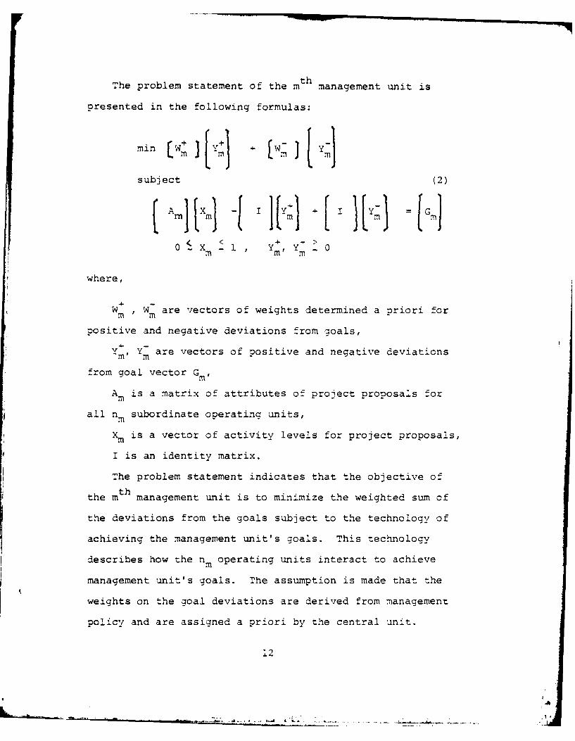
The problem statement of the mth management unit is

presented in the following formulas:

subj ect (2)

wher) I ' YXm m' m

m'm

positive and negative deviations from goals,

Y m, Ym are vectors of positive and negative deviations

from goal vector Gmy

Am is a matrix of attributes of project proposals for

all n m subordinate operating units,

Xm is a vector of activity levels for project proposals,

I is an identity matrix.

The problem statement indicates that the objective ofth

the m management unit is to minimize the weighted sum of

the deviations from the goals subject to the technology of

achieving the management unit's goals. This technology

describes how the nm operating units interact to achieve

management unit's goals. The assumption is made that the

weights on the goal deviations are derived from management

policy and are assigned a priori by the central unit.

12

i

Ruefli utilizes the following dual problem to generate

shadow prices. A negative shadow price means that the particu-

lar management unit has failed to meet a goal and positive

shadow price indicates that the management unit has exceeded

the goal.

max (Gm I mJ

subject A }T m 1 (2)

0

-~M [i (~34I: HA Lw;unrestricted

Shadow prices are passed up and down by management units.

These shadow prices are the inputed values of the goal

constraints. Operating units generate alternative proposals

for their superior management unit in response to the shadow

prices of the management unit.

The problem statement of the jmth operating unit is

illustrated by the following formulation:

(3)subj ect (j A F

m -105m

13

... ,__.. . ... .. . .. .... .. .. . . .________- __- _____ + . . k: . . , -_. .... -. - - +i' _+ .- -...

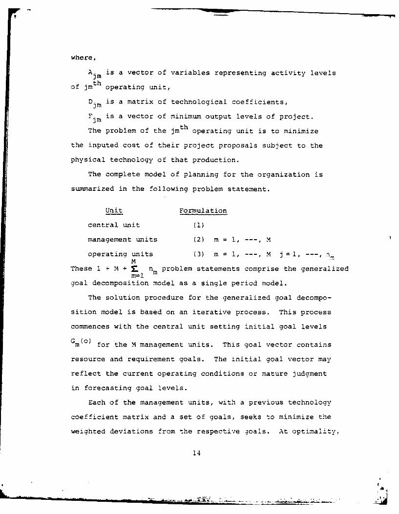
where,

Ajm is a vector of variables representing activity levels

of jm t h operating unit,

Djm is a matrix of technological coefficients,

Fjm is a vector of minimum output levels of project.

The problem of the jmth operating unit is to minimize

the inputed cost of their project proposals subject to the

physical technology of that production.

The complete model of planning for the organization is

summarized in the following problem statement.

Unit Formulation

central unit (1)

management units (2) m = 1, --- , M

operating units (3) m = 1, --- , M j1, --- , nM

These 1 + M + E. nm problem statements comprise the generalizedm=1

goal decomposition model as a single period model.

The solution procedure for the generalized goal decompo-

sition model is based on an iterative process. This process

commences with the central unit setting initial goal levels

G (o)m for the M management units. This goal vector contains

resource and requirement goals. The initial goal vector may

reflect the current operating conditions or mature judgment

in forecasting goal levels.

Each of the management units, with a previous technology

coefficient matrix and a set of goals, seeks to minimize the

weighted deviations from the respective goals. At optimality,

14

AI '-A- - -j A . .~ ~ . - L

the dual variables to this problem solution are the shadow

prices. Each management unit responds to the central unit

with a proposal of shadow prices. This vector of shadow

prices is provided to each of the operating units of the

.1 respective management unit and to the central unit.

Having received a vector of shadow prices for this

iteration, the operating units seek to minimize the inputed

cost of their proposals. This optimal solution yields a

new proposal for their management unit. This new proposal

is sent to their respective superordinate management unit

for the next iteration.

After receiving the shadow prices from the subordinate

management units, the central unit uses the shadow prices

to generate new sets of goal levels G m These goal vectors

are transmitted to the management units again.

Provided with a new technological coefficient matrix

by their respective operating units and goal levels by

their central unit, each of the management units optimizes

the revised program generating a new vector of shadow

prices. It is important to remember that shadow prices are

variables for the management units while they are considered

fixed by the central unit and operating units.

This process continues until the deviations from the

management unit goals are within prescribed tolerance limits

or at a minimum and no adjustment of goal levels on the part

of the central unit or modification of proposals on the

part of the operating units will yield a net decrease in

15

the deviations from the goal levels for the organization as

a whole. The iterative solution procedure is described in

Fig. 2.

Ruefli indicates that there are three types of externali-

ties possible in the generalized goal decomposition model.

The first type involves interdependence among operating units

subordinate to the same management unit. The model assumes

that these interdependencies are expressed in the constraints

of the relevant management unit's problem statement. The

second type of externality is present when the goal levels

of the mth management unit are dependent on the goal levels

of one or more of the other management units. The constraints

of the central unit are assumed to express these relationships.

The third type of externality arises when levels of project

characteristics are interrelated for operating units with

different superordinate management units. The central unit

then passes down upper limits on goal levels in the initial

conditions in order to rectify this problem.

If there are no technological and goal dependencies,

then the entire process will reach an optimum in a finite

number of iterations.

16

a) a..3,-. ,~

U) CU)1) ~

0~ ~*-4 t' C)4-. - -4 a) 4~4 t -

~ .v ~ a)C) -' .- -~-4 C~N pa. 4 ~ > *~

a) ~~a)~a)a)~ +-, - -

- -4

a)a) 3U) U) 0

U) 4- 2) -- - ~ -~ -~ U) .1

I) - -~ C '~ C C -~

4.- + U) ~J "~ C -~

4-. 0 a) *- - U) a)o '..-~ A 3 ~ U) +-~ + 2) U)

OW '3) a) QCU) - ~3C) a) '-~.- >

.4-4 -4 ~ '3)~) a) 0 ~ ~-. a) -'- > U) 4~4 C.. U) U)

.4-4 a) a) - a) -4-4 - ~ +~ 4~4 2)- C) U) a) C) - 11 U)

- -4' 0 a) -4 U) a) C.. CU) ," -. '-4 A a) H *;-' U) a) ~Z.

4---

U) ~.) '> ~3 a) a) :4 - U) a)0 ~ a) ~.. -~ :4 4z. *- - -

'-' *r-U) :4

a)a.4 U) -J

'Z V0 '-4 ~) C) - V-~ r~ *~ -~ .4-

4-. 444 0U) U) -. C.. U) A Ca) 2) -4 -'--~*'- -C) > '. 4 -~U) a) U) ... U)

C, -, ~ - 4- 1)

- -. '3 ~ U)- a... oU) 1 a) .~ a) .0..

~ 0 1 a)U) >0 a) '3 '3) ~

a) 0 tOO..

I 0- 4-' C.

- 73

1)2.) > C- 1)-

4~4 I--3) -

-I, ~L) -

'3 - 3 4- Cl )- 3) - 3) C

U *-4 - -

. - - K1 ~ K-

tO.~ '- K~ K~747 1 jU.T ~'U

III. MULTIPLE PERIOD PLANNING APPROACH OF GENERALIZED GOALDECOMPOS IT ION MODEL

In the previous chapter, Ruefli's generalized goal decom-

position model has been presented as a single period planning

model. Many organizations do exist over long periods rather

than in just a single period. Consequently, in the real

world, a lot of goals and objectives of an organization are

concerned with a planning horizon that encompasses more than

a single period. If the planning period is restricted to one

period, it is virtually impossible to make a genuine evalua-

tion of the alternatives in the decision process because

there can be lack of information between periods and between

each level of the organization.

If it is assumed that there are no interdependencies

among planning periods, then for each of the planning periods

under consideration, a single period model exists. Since

these problems have been assumed to be independent, then

they may be solved separately to yield a series of programs

for each period. This represents a case of suboptimization

within planning periods, and may yield some plans that are

undesirable from the long run point of view.

If the decision maker's horizon is extended to the next

period, he can do little more thian make incremental adj ust-

ments in the existing plan. The r~re later planning periods

are considered, the more adjustments can be made. Also,

18

this feature of multiple period planning can provide some

perspectiveson the future direction that are anticipated.

This section will be concerned with the extension of

the generalized goal decomposition model to do multiple

period planning of the organizations.

A. LINEAR FORMULATION OF MULTIPLE PERIOD PLANNING MODEL

The solution of the generalized goal decomposition

model is dependent on the structure of the organization.

The change of organizational structure may be considered as

a variable over the planning periods; that is, for example,

a certain operating unit is shifted to another management

unit. The results of the plan can be different from previous

ones. Therefore, it is necessary to assume that the structure

of the organization does not change over the time periods

and to assume that both central unit and management units

have control over the whole planning periods in the same

assumption of the generalized goal decomposition model, and

further to assume that the objective functions and constraints

of all levels of organization are linear functions because

of the cmtoutation algorithm. From these assumptions, the

problem statements of the central unit can be presented as

follows:

T M

t1l m--l M1-

19

s.t. (cost goal)

T M

t=l m=l mt Gmt1

s.t. (non-cost goal)

M

m: G [G t=l, T (1-3)

{G3t ) + = hmti j t 1, -,- - T-1 (1-4)

m= 1 1

mt

whez e,

t represents the planning period,

m represents the management unit,th

is a vector of shadow prices generated by the mn

management unit in the tth planning period, thGmt is a vector of goal levels assigned to the m

management unit in Uie tth planning period. The cost goals are

not contained in the vector Gmt of Equation 1-4,th

Pmt is a matrix of the m management unit's joint

utilization of the organizational goals in the tt h planning

period, The i th row relating to the cost goal is not included

in the Pmt?

20

!

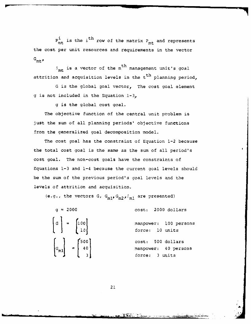
P is the i th row of the matrix Pm and represents

the cost per unit resources and requirements in the vector

G mtPS mt is a vector of the m thmanagement unit's goal

attrition and acquisition levels in the t th planning period,

G is the global goal vector., The cost goal element

g is not included in the Equation 1-3,

g is the global cost goal.

The objective function of the central unit problem is

just the sum of all planning periods' objective functions

from the generalized goal decomposition model.

The cost goal has the constraint of Equation 1-2 because

the total cost goal is the same as the sum of all period's

cost goal. The non-cost goals have the constraints of

Equations 1-3 and 1-4 because the current goal levels should

be the sum of the previous period's goal levels and the

levels of attrition and acquisition.

(e.g., the vectors G, G mlP Gm2f ml are presented)

g -2000 cost: 2000 dollars

G [00oo manpower: 100 persons

11 10O force: 10 units

P500 cost: 500 dollars

G =m 40 manpower: 40 persons

21

°500 cost: 500 dollarsGm2 = 4 5 manpower: 45 personsL force: 3 units

4 5 manpower: 5 persons

rml 0 force: 0 units

In the central unit's problem, we have assumed that the

central unit has information about the global goal vector G

and has set all of the goal levels GII, .... G mt for the M

management units in each planning period, in light of their

relationship to each other and the global goals, and in light

of the information about their needs supplied by the manage-

ment units. The central unit's problem is to maximize the

inputed values of all of the management units' output

subject to the global goals.

The problem statements of the mth management unit is

presented in the following equations:

min Z ( IW t] +Y Wmt ¥mT + 41 At) [ -t=l

s.t.

A X 01 Y +s 'ml mlI '

A X 2 2

22

A

Y ml ml

Y m2+!

X 0

a- - .

mt Ymt Ymt

where,W+

Wmt W are vectors of weights assigned to the posi-m mt

tive and negative goal deviations in the tth planning period,y+

Ym' Ymt are vectors of positive and negative devia-

tions from the goal vector Gmt,

A is a matrix of attributes of project proposalsmt

for all 7i subordinate operating units in the tth planning

period,

Xmt is a vector of activity levels for the project

proposals in the tth planning period,

I is an identity matrix.

The objective function of the mth management unit is

the sum of all single planning period's weighted goal devia-

tions from their respective goal levels. The large matrix

equation of the constraints is composed of the constraints

of each single period; that is, the generalized goal decompo-

sition model. The management unit's problem is to minimize

its aggregate weighted goal deviations from each planning

period's goals which are set by the central unit, subject to

the technology of achieving the management unit's goal.

23

4- - y+ -

(e.g. the vectors Gm, Gm2 ml' Y m' ' Y areml' m' mi, ml'm2' m2 ar

presented)

G1 [5001 cost: 500 dollarsG mf 40 manpower: 40 persons

3 force: 3 units

5015 cost: 50 dollars

[m24 = manpower: 4 persons

force: 3 units

50 cost positive deviation:

01 manpower positive deviation:

10 persons

force positive deviation:

0 units

y = ml force negative deviation:

1 unit

~0

= 0m2b 0

[1 30J cost negative deviation:

5 Imnoe 30 dollarsnImanpower neaative deviation:

5 persons

The formulation of the jmth operating unit's problem can

be described as follows:

t=l

24

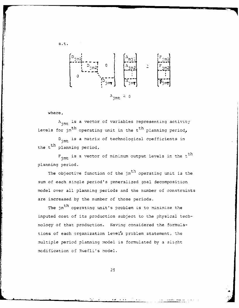
S.t.

D. ASDmjl "ml

D. 0 A. F

0

j y tjiry tfmA

Ajmt - 0

where,

A mt is a vector of variables representing activity

th thlevels for jm operating unit in the t planning periodp

Djm t is a matrix of technological coefficients in

the tth planning period,

Fjmt is a vector of minimum output levels in the

planning period.

thThe objective function of the jm operating unit is the

sum of each single period's generalized goal decomposition

model over all planning periods and the number of constraints

are increased by the number of those periods.

The jmth operating unit's problem is to minimize the

inputed cost of its production subject to the physical tech-

nology of that production. Having considered the formula-

tions of each organization levels problem statement, the

multiple period planning nodel is formulated by a slight

modification of Ruefli's model.

25

'11

In the practical point of view, it is difficult to use

the simplex method of the linear programming for the solution

method of the linear formulation of the multiple period

planning model because the information required is unclear

and changing, furthermore the externalities mentioned in the

previous chapter are more probable due to many variables and

constraints in the problem statements of each level of the

organization.

B. DYNAMIC FORMULATION OF MULTIPLE PERIOD PLANNING MODEL

In the multiple period planning model, the objective of

the management unit's problem is the minimum weighted goal

deviations from the assigned goals as a whole. The global

cost goal is distributed over all planning periods and

then distributed over all ninagement units. The non-cost

goals are distributed over all management units and these

goal levels are available in every period without changing.

From this point of view, the multiple period planning

model can be described in the following simplified formula

by using the planning period's subscript t:

Tmin E r t (Gt, gt (2-1)

t=l

s.t. (cost goal)

Tgt & g (2-2)

t= 1

s.t. <non-cost goal) (2-3)<

G -Gt>

26

A

where,

t represents planning periods,

G is a non-cost goal vector assigned for centralt

unit in the tth planning period,

G is the global non-cost goal vector,

gt is the cost goal levels for the central unit in

the tt h planning period.

g is the global cost goal levels.

rt(Gt, gt is a function of Gt and gt' i.e., the

weighted goal deviations from the management units' goal

vector.

In the tth planning period, the goal vector Gt and the

cost goal g assigned by the central unit vary, the weighted

goal deviations r (Gt, gt) will have different values.

Furthermore, the objective function for all the periods is

an additive form of each single subperiod. Since the opti-

mization problem can be decomposed into recursive equations,

then the system can be described in terms of a number of

state variables. That is, separability and monotonicity

conditions are satisfied because of the additivity of the

objective function.

If we pick up planning periods for stages, then the

stage diagram can be presented in Fig. 3.

where,

stage T corresponds to the first planning period,

stage 1 corresponds to the last planning period,

27

• _. .... . . . ,, , ... . .. , .• ,6 A ... . . . _ - ...,

-4

II

x x

I* -

-*-~ I -

C)

x

II -~o

-~ I I .1

* 1 -~

-, I

*1

*' .

xis a state variable vector representing the

amount of goals left to be allocated to stages t, t-1,

----

G t is a decision variable vector representing

the amount of goals to be allocated in stage t,

xis a state variable relating to the cost goal in

stage t,

g is the global cost goal to be allocated over all

planning periods,

G is a global non-cost goal vectorl

r t(G t) is immediate return function in stage t,

9is the decision variable relating to the cost goal

in stage t.

All of the global goal levels are available to use in

stage T (the first planning period), therefore the state

variable vector XT is the global goal vector G and the state

variable x T of the cost goal i.s the global cost goal g.

The state variable vector X" of the non-cost goals is

4 just the global goal vector G because the amount of goal

levels left in stage T-1 is still the global goal vector.

But the state variable xl of the cost goal is xT g The

amount of cost goals allocated in stage T should be sub-

tracted from the state variable x T because the state variable

Xl is the amount of cost goals left to be allocated toT-the stages T-1 - ----- 1. The state variables in the other

stages can be produced from the formnulas in the staqe

di agramn.

In each stage, the state variable vector Xt and the

decision variable vector Gt are the input variables and the

return function r t(G t ) is the immediate output. The decision

variables are presented in the following equation derived

from the central unit's problem in the Ruefli model.

Gtl = Lmt GmJm=l

where,P is a matrix of the mth management unit's joint

utilization of the organizational goals in stage t,

Gmt is a vector of goal levels assigned to the mth

management unit in stage t.

The objective of the multiple period planning model is

to minimize the goal deviations from each management unit's

goal levels in each period. In this sense, the return

function can be presented in the following equation which is

the sum of all management unit's objective functions in the

generalized goal decomposition model.

rM=l + m y+ +(-)[t~{+ (WG t) [ (Wt ]i

where,

W+ Wmt are vectors of weights for positive and

negative deviations from goals in stage t,

yr' Ymt are vectors of positive and negative devia-

tions from goal vector in stage t.

Up to this point, stages, state variables, decision variables

and return functions have been defined. The key to all n:

30

~~~~~~~~~~~. ... ......... ... : - . • . . -_-____.- ________' ,'

programming problems is writing a recursion equation for the

optimal return function, since the objective function of this

model is assumed to have a linear relationship to the single

period's outputs.

The corresponding recursion equation of multiple period

planning model can be presented as follows:

ft (Xt min I r t(Gt) + ft-1(Xt-l)I

0 - - Xt , where the inequalities of

Equations (-2) and (-3) are

Gt > Xt , where the inequalities of Equations

(2-2) and (2-3) are >.

where,

rt(Gt) is the immediate return function,

ft-l(Xt-l) is optimal return function for remaining

stages t-l, ...., I with the remaining goal levels Xt_1 .

In the recursion equation defined above, the central unit

has to choose the goal vector Gt to minimize the sum of

immediate return and the optimal return, which is the best

we can do for the remaining stages t-l, --- , 1 with the

remaining goals Xt_1, Since some parts of the goals have

been used already in the previous stages, the rest of the

goals are

The important feature of the recursion is that we do not

have to think about the decisions G ---- , G , which give

Z (Xt_ ) , thus we have a single period ptimization over

t , Due to Nemhauser, an optimal set of decisions must be

31

A

optimal with respect to the outcome which results from the

first decision.I The standard solution process has the following steps.

I. Compute f (X ) for all possible values of X, by

using the generalized goal decomposition model and store

the results.

f I(X) min r (G1

0 - G - X 1or G 1>X

2. Compute r 2 (G 2 ) for all possible values of G 2 by

using Ruefli's single period model in stage 2 and then f 2 (X 2 )

for all values of X 2 by using the following recursion equation

in stage 2 and store the results.

f (X) min ~r(G ) + f (X1)

2212 2 2 12

3. Continue recursion computations f 3 (X 3),- ----- f T(Xm).

4. Compute the decision variables by the backwards

track of the optimal solutions.

in the practical point of view, it is difficult to follow

the above solution process, because there are many decision

variables in each stage. If there are more goal elements

than one, then we have to compute every possible combination

of the goal elements and store the results. For example,

if there are three goal elements and each of these goal

elements has 100 possible values, then there are 100

combinations of these goal elements. This is known as the

curse of dimensionality. The computations in this dynamic

32

program increase exponentially with the number of the

variables, but only linearly with the number of stages.

Due to this computational difficulty, we have to consider

another solution process reducing the burdon of computation.

C. SOLUTION METHOD OF MULTIPLE PERIOD PLANNING MODEL

The linear and dynamic formulations are presented in the

previous sections. The linear formulation cannot be solved

simultaneously by the simplex method of linear programming

because of a lack of information, and too many variables and

constraints in the problem statements of each level of the

organization. Also, the standard dynamic programming

approach is not available for the solution method of the

multiple period planning model due to many decision variables

in each stage.

Before attempting to determine a suitable method, it

is necessary to understand the nature of the multiple period

planning model and the generalized goal decomposition model.

The optmitation is to minimize the weighted goal deviations

from the assigned goal levels. If the goal levels are too

large or small, the weighted goal deviations are large. Con-

versely, if the goal levels are appropriate in each stage,

then the goal deviations will reach a minimum.

goaldeviations

i_ goal levelsA M B

Fig. 4

33

!

In Fig. 4, the goal deviations of point M are minimum

and smaller than those of A and B. From this feature of the

model, we can reasonably assume that the weighted goal devia-

tions of each stage problem are convex functions of the goal

levels. Therefore, the following search algorithm can be

used instead of the previous standard method. The search

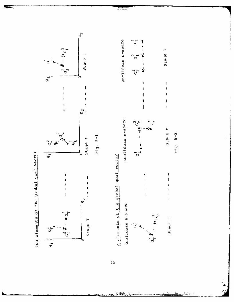
points of each stage are presented in Figs. 5-1 and 5-2,

where g, and g2 are the elements of the global goal vector G

to be allocated over all stages.I tt hGt is the stage's initial iteration point assigned

by the central unit with the existing information, Gis thet

tt h stage's second iteration point determined by the search

algorithm, etc.

In the case of two goal elements, the feasible region of

each stage is the first quadrant determined by the two goal

elements in Fig. 5-1. The goal deviations of these feasible

points build up a convex plane in three dimensional space.

In the n goal elements case, the feasible region of each

stage is the Euclidean n-space and the outputs of these

points also form a convex hynerplane in the Euclidean n+l

space with a projection shown in Fig. 5-2.

1 _'If the initial points G,, ---- G Gi are the optimal

solution points, then movina to any direction from these

points increases the goal deviations. if tne oal deviations

of stage T are large because of the extra amount )f oal

levels, the goal deviations of stage T-1 are also large iue

to small amount of 7oal levels, and further those or all

34

t I I -

-4- lyC

>44C14

(1,-4

CN)

C.3 413

04 '- 1

r-4_ _ __ __ _ 1& -4

41 00 41..) u

00

-4-

C)l

0 -4

& *~-4fn 010

C) C)

35

remaining stages are optimal points, then the minimum goal

deviations are produced to the decreasing direction of goal

levels in stage T and the increasing direction in stage T-1.

This feature of the model can be used to find the successive

iteration points without computation of all feasible points.

The central unit determines the initial points G11T

G with the existing information. These points are the

central unit's global goal 'Levels of the generalized goal

decomposition model; therefore Ruefli's model exists in each

stage. The optimization problem can be solved by using the

generalized goal decomposition model for stage T through

stage 1. The management units produce the weighted goal

deviations and the positive and negative goal deviation vectors

of all stages at the last iteration of each stage problem.

The goal deviation vectors are sent to the central unit

and the management unit's cost goal weighting factors are

also transmitted to the central unit. The central unit has

to determine the second iteration points C~ GI-- c o

reduce the management units' weighted goal deviations.

Therefore, the central unit uses ~h~information transmitted

by the management units to choose the second iteration points.

The central unit's process choosing the second iteration

points is presented in the following pages.

To determined the second iteration points, it is needed

to compute each stage's positive and negative deiaticn

vectors, the difference vector of the c)ositive and necative

deviations, the total positive and negative cost goal deviations

36

and the differences of the total positive and negative cost

goal deviations.

j = tmt t, ---- T (3-1)

m=l

[ Pm t [Y t 1 , -, T (3- )

(non-cost goal)

T+ +

Y y + (cost goal) (3-4)

t=l

T

Y = Yt (cost goal) (3-5)

t=l

y D y -y+ (3-6)

where,Yt' Y tare the positive and negative goal deviation

vectors including the cost goal deviations in stage t,

r+', Yt are the mt h management unit's positive andmt mt

negative goal deviation vectors in stage t,

Pmt is the mth management unit's joint utilization

matrix in stage t,

tD is the difference goal deviation vector in stace t,

37I

Yt' Yt are the total positive and negative cost .uoal

deviations over all management units and over all stages,

yD is the differences of the total positive and

negative cost goal deviations.

The positive and negative goal deviation vectors Y+ Y in

each stage are computed from Equations (3-1) and (3-2), and

then each stage's difference goal deviation vector is acquired

from Equation (3-3). The total positive and negative cost+

(

goal deviations y , v are obtained from Euations (3-4) and

(3-5), and the total differences of the cost goal deviations

are produced from Equation (3-6).

The element of the difference goal deviation vectors can

be positive, negative or zero. The positive element repre-

sents that the goal levels are too large, the negative element

means that the goal levels are too small and the zero values

of the element indicate that there is no shortage or surplus

of the goal levels.

In the case of the positive elements of the vector Y1,+

there is no need to modify the elements of the vector Yt

but the element of the vector Yt should be examined whether

the goal deviations of each element can be reduced in the

next iteration. On the contrary, in the case of the negative

elements of the vector Yt, no restrictions exist in the

elements of the vector Yt while the elements of the Y,

should be considered whether the adjustment of each element

is needed or not. if the elements of the vector Y are

positive and the corresponding inequalities of the

38

.l.

Equations (2-2) and (2-3) are - (less than), or the elements

Dof the vector Y are negative and the corresponding inequali-

ties are > (greater than), then the elements of the vector

Y in the former case and the elements of the vector '-t + in

the latter case do not need any adjustments because the

elements of the global goal vector G represent the maximum

levels in the case of less than ineaualities and the minimum

levels in the case of greater than inequalities.

The central unit has each stage's positive and negative

deviation vectors, the difference vector, the total positive

and negative cost goal deviations and the differences of the

total goal deviations. But the central unit also needs the

actual goal levels left in the first iteration. Each stage's

non-cost goal levels and the total cost goal levels left can

be computed from Equations (3-7) and (3-8).

[1 = [G - [G t = 1, ---- (3-7)

TR 9"- (cost goal) (3-8)

t=1

where,

g is the global cost goal,

RGt is the remaining goal vector in stage t,R

g is the total remaining cost goals,

i s the t h stage's cost goal assigned by the

central unit for the first iteration,-1 tththe t stage's non-cost :;oals for the first

iteration.39

_ .- A................. .. .... - "T . .

The elements of the vector GR can be positive, negativeR

or zero. The positive element of the vector Gt means thatt

the goals are underdistributed in stage t, the negative

element indicates that the goals are overdistributed and the

zero values represent that there are no surpluses or

shortages.•D

f the elements of the vector Yt are positive and the

corresponding inequalities of the Equations 2-2 and 2-3 are

>(greater than), then the values of the elements of the

D Rvector Ytand Gt are subtracted from the elements of the

vector Yt to meet the global goal constraints at least

because the elements of the vector GR are negative.tD

If the elements of the vector Y are negative and the

corresponding inecualities of the Equations 2-2 and 2-3

are _ (less than), then the values of the elements of the

vector and G are added to the elements of the vector

Y to meet the global goal constraints at most because thet R

elements of the vector Gt are positive.

This modification of the vectors YT, --- ', Y' ---' Y

N+ vN- N4-produces the new vectors YT , , T --- ' of the positive and negative

I ~T ' 11

goal deviations ineach stage. The new elements v N+ and y

of the total positive and negative cost goal deviations

are produced from the same process using the total remaining

R Dcost goals g and the total difference goal deviations v

The elements of the vector YN+ represent that these

positive goal deviations can be reduced by adding the

additional ,-oals. The elements of the vector YN indicate-t

40

.... . .. . ~ " " .. . . - - - . . . ... - [, -.. ,, L U T _. '- . .. . . .. .. . . . .

that these negative goal deviations can be subtracted from

the goals distributed over stage t in the previous iteration.

If it is assumed that the global goal vector G has K

elements, then the following Equations 3-9 through 3-12 can

be used to produce the positive and negative ratios.N+v~t

ti -4- t=l, - (non-cost goal) (3-9)

Yti tl,..,T

N--i= --- , K-1 (non-cost goal) (3-10)' - Yti' 'rti - t=l, --- , T

Yti

r + (cost goal) (3-11)r +y

N-r (cost goal) (3-12)

y+ th

where, is the i element's ratio of the vectors Y+ andt+ - th N

Yt and rti is the i element's ratio of the vector Yt and

Y The ratios of the total positive and negative cost goal

deviations can be used for all stages; therefore each stage's

vectors + - R , - , where the vectr 3+

ri +for ail i, are produced fr.om Equations 3-9 through 3-12..... + y ,- -

If the ith elements of the vectors YT, --- Y ,

y are zero, then the it h positive and negative ratios are

zero because the zero cannot be used as a denominator.

These zero values mean that there is no goal deviations at

all.

41

The central unit has to consider the zero values of the+ -

cost goal ratios r , r-. The zero values are produced for

the following two reasons:

1. The numerator and denominator are both zero.

2. The numerator is zero, but the denominator is

positive.

In Case 1, there is no need to adjust the existing cost

goal levels because the positive and negative deviations

are zero. In Case 2, the central unit cannot distribute

more cost goals over the stages and subtract the extra goals

from the stages with surplus goal levels, but the central

unit can transfer the goal levels from the stages with large

weighting factors to the other stages with small weighting

factors to reduce the weighted goal deviations of the manage-

ment units. Therefore, the ratios of the cost goal in Case 2

should be modified by using the weighting factors:

M+ 1 -W+Wt + W +m t=l, ... ,T (3-13)m=l

M1* = Wmt t=l, .... , T (3-14)m=l

where, W+ W- are the tth stage's positive and negative

weighting factors about the cost goal and W+mnt' Wmt are the

mth management unit's positive and negative weighting factors

in stage t. Each stage's positive and negative weighting

factors about the cost goal are the average of all management

units' weighting factors. These weighting factors obtained

42

-ALL

from Equations 3-13 and 3-14 can be different from stage to

stage in spite of the same cost goal.

If the positive ratio r +is the Case 2, then it is needed

to choose the positive cost goal deviation with the largest

weighting factor among yT -+ - y + and then to select the

corresponding element of the weighting factor among

--- , w 1 It is also needed to select the smallest element

of the weighting factor. if the wT is selected for the former

and the w + is for the latter, then the positive cost goalt

ratio of the vector R + is replaced with 1 and the positivet

cost goal ratio of the vector R+is replaced with -1, andt

also the positive cost goal deviation y4+is replaced with

the positive cost goal deviation y +to transfer the cost

goal levels from stage T to stage t.

The positive cost goal deviations in stage T can be

eliminated, while the positive cost goal deviations in

stage t will be increased by this replacement of the positive

ratios and deviations. However, the total weighted goal

deviations of all stages should be decreased. This replace-

ment is performed in the negative cost goal ratios and

deviations by using the same process. If the case 2 does

not exist, then the positive ratios r+ r t are all therT' I

same and the negative ratios r T r-- r1 have also the

* same values.

43

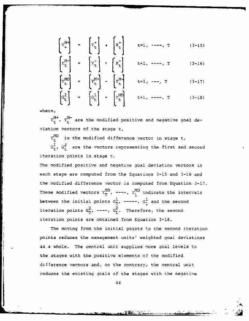
I [+ . R + t=1, - ----- T (3-15)

+ t1 t =,--,T(-6

t t ...tc 1

(G G + [YMI~ t=1, - ---- , T (3-18)

where,

M+ M-Y , Yt are the modified positive and negative goal de-

viation vectors of the stage t,

t is the modified difference vector in stage t,

1 2Gt, Gt are the vectors representing the first and second

iteration points in stage t.

The modified positive and negative goal deviation vectors in

each stage are computed from the Equations 3-15 and 3-16 and

the modified difference vector is computed from Equation 3-17.

These modified vectors YMD yMD indicate the intervals1 1

between the initial points GT,. ------, G and the second

iteration points GT, ---- , G 1 . Therefore, the second

iteration points are obtained from Equation 3-18.

The moving from the initial points to the second iteration

points reduces the management units' weighted goal deviations

as a whole. The central unit supplies more goal levels to

the stages with the positive elements of the modified

difference vectors and, on the contrary, the central unit

reduces the existing gcals of the stages with the negative

44

- . . . ". .. - - " . .. " " " ' - - ---: ', -"- £ [£ . - ,'r , -... . .... ' . .. ,.. T . - " A .

elements. if all elements of the vector Y+. are zero, then

the t th stage's first iteration point G 1 is the same as thet

second iteration point G 2I t*

If the second iteration points G 2 --- G2ardermn ,

then each stage problem can be optimized by the feedback

process of the generalized goal decomposition model. When

the optimal solutions about the second iteration points are

obtained, the management units send the positive and negative

deviation vectors and the positive and negative weighting

factors about the cost goal to the central unit in each stage.

The central unit uses these results to choose the next ;.tera-

tion points.

This process continues until all elements of the modified

difference vectors ---- , YM~Darzeo ThsensttT ae er. hi man ta

there is no movement of the iteration points in the next

iteration and also the current solution is optimal. If the

convexity assumption of each stage problem is correct, then

the management units' weighted goal deviations become smaller

and smaller in accordance with iteration. Eventually the

minimum weighted goal deviations should be achieved by this

iterative search algorithm in a finite number of it.erations.

The iterative search algorithm produces the multiple

period plan based on the existing information at the begin-

ning of the first planning period.

In the real world, the information in the far planning

periods are unclear and do not remain constant, but grow out

of the experiences and external environment in accordance

45

with the moving from period to period. The information in

the near planning periods is more clear and unchanging than

the far planning periods. Therefore, the plan is updated

by excluding the first planning period at the beginning of

the second planning period while bringing in the T+lst planning

period. This modification of the plan -7an be made at the

beginning of every planning period if it is needed.

46

IV. SUMMARY

In this thesis Ruefli's generalized goal decomposition

model has been extended to make a more realistic evaluation

of the alternatives in the decision making process of an

organization from the long run point of view. The multiple

period planning model in the three level organization is

formulated with linear goal deviations by introducing the

goal programming method used in Ruefli's model. The global

goals are distributed over all planning periods and then

over all management units. The management units' minimum

weighted goal deviaitions are obtained from the optimal

distributions of these goals. Dynamic formulation using

the generalized goal decomposition mnodel for each single

period problem is also presented.

The linear formulation cannot be directly used to obtain

the optimal solution due to lack of information and too many

variables and constraints in the problem statements of each

level of the organization. The dynamic formulation also

cannot be directly used because of too many decision variab~es

in each stage.

An iterative search algorithm is presented as an appro-

priate solution method of the dynamic formulation of the

multiple period planning model. In the iterative search

algorithm, the generalized goal decomposition mnodel is used

47

to solve the problem of each planning period in every

iteration.

48

LIST OF REFERENCES

1. Heal, G. M., The Theory of Economic Planning, North-Holland/

American Elsevier, 1973.

2. Crecine, J.P., Studies in Budgeting, North-Holland Publish-ing Company, 1971.

3. Ruefli, Timothy W., "A Generalized GoalDecomposition Model,"Management Science, Vol. 17, No. 8, pp. B505-B518, April

1971.

4. Ruefli, Timothy W., "Behavioral Externalities in Decen-tralized Organizations," Management Science, Vol. 9, No. 5,pp. B649-B657, June 1971.

5. Ruefli, Timothy W., Planning in Decentralized Organizations,Ph.D. Thesis, Carnegie-Mellon University, 1969.

6. West, Lorenzo, III, A Model of Organizational DecisionProcess, M.S. Thesis, Naval Postgraduate School, March1972.

7. Sweeney, Dennis J., "Composition vs. Decomposition: TwoApproaches to Modeling Organizational Decision Process,"Management Science, Vol. 24, No. 14, October 1978.

8. Smithies, Arthur, PPBS, Suboptimization and Decentraliza-tion, Rand, RM-6178-PR, April 1970.

9. Nemhauser, George L., Introduction to Dynamic Programming,John Wiley and Sons, Inc., 1966.

10. Beckman, Martin J., Dynamic Programming of EconcmicDecisions, Spring-Verlag New York, Inc., 1968.

11. Dreyfus, Stuart E., The Art and Theory of DynamicProgrammina, Academic Press, Inc., 1977.

12. Zionts, Stanley, Linear and Integer Programming,Prentice-Hall, Inc., 1974.

13. Daellenbach, H.G., "Note on Multiple Objective DynamicProgramming," Operational Research Society, Vol. 31,No. 7, pp. 591-594, July 1980.

11. Halloway, Charles A., "Comparison of a Multiple-PassHeuristic Decomposition Procedure with Other Resource-Constrained Project Scheduling Procedures," ManagementScience, Vol. 25, No. 9, September 1979.

49 A

INITIAL DISTRIBUTION LIST

No. copies

1. Defense Technical Information Center 2Cameron StationAlexandria, Virginia 22314

2. Library, Code 0142' 2Naval Postgraduate SchoolMonterey, California 93940

3. Asst. Professor D. C. Boger, Code 54Bk 1Department of Administrative SciencesNaval Postgraduate SchoolMonterey, California 93940

4. Department Chairman, Code 55 1.Department of Operations ResearchNaval Postgraduate SchoolMonterey, California 93940

5. Professor C. R. Jones, Code 54 1Department of Administrative SciencesNaval Postgraduate SchoolMonterey, California 93940

50