1

EFUW Summary

Andreas Biri, D-ITET 06.06.15

1. Introduction

Units 1J = 1 Nm = 1 Ws = 1 , 1 � = 1 � 1 W = 1 ��� = 1 VA , 1 = 1 �⁄ = 1 �/�� 1 V = 1 W A⁄ = 1 � ⁄ = 1 �� , 1 = 1 �� 1 � = � ��⁄ = 1 � ��⁄ , 1� = 1 ⁄ = 1 ��/

Natural constants �� = �. !"# ∗ �"%�& ', � ' = !. #( ∗ �"�) � �* = 9.11 ∗ 10%-. /0 , 0 = 9.81 � �%� 2 = 2.99792458 ∗ 107 �/� 8" = ). )9( ∗ �"%�# :; <=> , ?# = �8" @"

A" = (B ∗ �"%C DE ∗ F ∗ G%# ∗ H%#

Basic Properties

�IJ, KL = M N OIJ, KL + QIJ, KL ∗ RIJ, KL S

NOS = �⁄ , NRS = � ��⁄ , N�S = � = /0 �/��

Magnetic field is relative counterpart of electric field

OITU, KL = M4VWU XYZ[T\� + T\2 ]]K ^YZ[T\�_ + 12� ]�]K� YZ[ `

Charge density: aITL = ∑ Mc dN T − Tc Sc

Current density: fITL = ∑ Mc Tcgc dN T − Tc S

�IT, KL = h i aIT, KL OjkIT, KL + lkIT, KL m RjkIT, KL n ]o

Poisson: ∇ OImL = − ∇� qImL = rIsLtu

2. Maxwell’s Equations

Pre-Maxwellian Electrodynamics

Gauss’ law

h OjkIT, KL ∗ Yjk ]vwo = 1WU h aIT, KL ]o = xWU

Faraday’s law / Induction law

h OIT, KL ]�wy = − ]]K hRIT, KL ∗ Y ]vy = z{cw

Ampere’s law

h RIT, KL ]�wy = |U hfIT, KL ∗ Y ]vy = |U }

No magnetic monopoles, zero flux & electrostatics

h RIT, KL Y ]vwo = 0, h fIT, KL Y ]vy = 0, h OIT, KL ]�wy = 0

Maxwell’s equations in integral form

h ~IT, KL ∗ Y ]vwo = h aIT, KLo ] h OIT, KL ]�wy = − ]]K hRIT, KL ∗ Y ]vy h �IT, KL ]�wy = h � fIT, KL + ]]K ~IT, KL � ∗ Y ]vy h RIT, KL ∗ Y ]vwo = 0

Maxwell’s equation in differential form

∇ ∗ ~IT, KL = aIT, KL → ∇ ∗ OIT, KL = aIT, KL/WU ∇ m OIT, KL = − ]]K RIT, KL ∇ m �IT, KL = ]]K ~IT, KL + fIT, KL "��J?��������" ∇ ∗ RIT, KL = 0

Continuity equation / conservation of charges

h fIT, KL ∗ Y ]vwo = − ]]K haIT, KL ]o ∇ ∗ fIT, KL = − ]]K aIT, KL

Displacement current

fw{�� = WU ]]K O

Interaction of fields with matter

Primary sources: 2ℎvT0�� a vY] 2�TT�YK� f

Secondary sources: �Y]�2�] 2ℎvT0�� �� ����]�

Polarisation P : � �IT, KL ∗ Y ]vwo = − � a���IT, KL ]o

Electric displacement : ~ = WU O + � = WU WZ O

Polarisation current: due to bound charges

f���IT, KL = ]]K �IT, KL N � S = /��

Magnetisation M : � �IT, KL ]�wy = � f���IT, KL ∗ Y ]vy

Magnetic field : � = .�u R − � N�/�S

R = |U |Z �

Magnetisation current: due to circular charges f��� = ∇ m �

Conduction current: due to free charges f��cw = � O

Total current f �  = fw{�� + f��cw + f��� + f��� = WU ]]K O + � O + ]]K � + ∇ m �

2

3. The Wave Equation

Inhomogenous wave equations

∇ m ∇ m O + 12� ]�O]K� = −|U ]]K ^ f + ]�]K + ∇ m � _ ∇ m ∇ m � + 12� ]��]K� = ∇ m f + ∇ m ]�]K − 12� ]��]K�

Homogeneous solution in free space

No material or sources: ∇�O − .�¡ w¡w ¡ O = 0

Else: ∇� O − c¡�¡ w¡w ¡ O = 0

Monochromatic waves

time-harmonic: oscillate with one fixed frequency OIT, KL = ¢� £ OITL ∗ �%{¤  ¥

Helmholtz equation ∇� OITL + /� OITL = 0 , / = ¦/2

Plane / homogenous waves OIT, KL = ¢� £ OU �± {¨∗Z % {¤  ¥

+ �/ ∗ T ∶ propagation in k-direction, outgoing waves − �/ ∗ T ∶ propagation against k-direction, incoming waves

Dispersion relation

/s� + /ª� + /«� = /� = Y� ∗ ¦�2�

¦ = 2V� , 2 = ¬ � , / = 2V ¬> O ⊥ � ⊥ / ‖ ¯ → O ∗ / = 0 = � ∗ / = O ∗ �

� = 1¦ |U I / m O L , �°T ±�vY� ²vQ� � = 1� ¦ |U I ∇ m OL , �� Y°K ±�vY� ²vQ�

Evanescent waves

If ³ /s� + /ª� ´ > /� , Kℎ� ²vQ� ��2°��� �QvY��2�YK: /« = ·¦� 2�> − ³ /s� + /ª� ´ ∈ � ℝ

OIT, KL = ¢� º OU �± { ³¨» s¼¨½ ª´%{¤  ∗ �∓ |¨À| « Á

Decay exponentially in z-direction, only near sources

Spectral representation

OIT, KL = h OÂIT, ¦L �%{¤  ]¦Ã%Ã

OÂIT, ¦L = 12V h OIT, KL �{¤  ]KÃ%Ã

OÂIT, −¦L = OÂ∗IT, ¦L , dImL = 12V h �{s  ]KÃ%Ã

Maxwell’s equation in Fourier form ∇ ∗ ~ÄIT, ¦L = aÅIT, ¦L ∇ m OÂIT, ¦L = �¦RÂIT, ¦L ∇ m �ÄIT, ¦L = −�¦~ÄIT, ¦L + l̂IT, ¦L ∇ ∗ RÂIT, ¦L = 0

Monochromatic waves

OÂIT, ¦\L = 12 N OITL dI¦\ − ¦L + O∗ITL dI¦\ + ¦L S

For time-harmonic fields, the Maxwell equations simplify: ∇ ∗ ~ITL = aITL ∇ m OITL = �¦RITL ∇ m �ITL = −�¦~ITL + fITL ∇ ∗ RITL = 0

Interference of waves

}ITL = ÇWU|U È OIT, KL ∗ OIT, KL É

Monochromatic: }ITL = .� ·tu�u |OU|�

|O|� = O ∗ O∗ = < O, O >

Evanescent: }ITL = .� ·tu�u |OU|� ∗ �%� ¨À «

1/� decay length for evanescent waves: Ë« = 1/I2 /« L

Field pair

}ITL = ÇWU|U ÈN O. + O�S ∗ NO. + O�S É = }. + }� + 2 ∗ }.�

Coherent fields: monochromatic, same frequencies

}ImL = }. + }� + ·WU |U> ¢� º O. ∗ O�∗ �{¨sI�ÌÍ Î¼�ÌÍ Ï L Á

If they are real and polarized along the z-axis

}ImL = }. + }� + 2 Ð}. }� ∗ cosN /m I��Y Ó + ��Y Ô L S

Visibility / “Interferenzkontrast”:

Õ = }��s − }�{c}��s + }�{c , Õ = 1 �°T }. = }�

}��s ∶ /°Y�KT�/K�Q ↔ }�{c ∶ ]��KT�/K�Q , ∆T = ¬/2

Period of interference: ∆ m = ¬ / Isin Ó + sin Ô L

Incoherent fields

The interference term vanishes due to ∆¦ = ¦. − ¦� }ImL = }. + }�

3

4. Constitutive Relations

Temporally dispersive: field depends on previous times

Spatially dispersive: field depends on other locations

~ÄI/, ¦L = WU WI/, ¦L OÂI/, ¦L RÂI/, ¦L = |U |I/, ¦L �ÄI/, ¦L

For time-harmonic fields ~ITL = WU WI¦L OITL RITL = |U |I¦L �ITL

For time-dependent fields

Can only be used in dispersion-free materials I WI¦L =W , |I¦L = | L , especially in vacuum.

Electric & Magnetic Susceptibilities W = I 1 + Ú*L �ITL = WU Ú*I¦L OITL | = I 1 + Ú�L RITL = Ú�I¦L �ITL

Conductivity f��cwITL = �I¦L OITL

Electric permeability

W = W\ + � �¦WU

¢�£ W ¥ = W\ : energy storage }�£ W ¥ = Û¤tu : energy dissipation

Helmholtz equation for isotropic materials ∇� OITL + /� OITL = ∇�OITL + /U� Y� OITL = 0

Index of refraction: Y = √W |

/ = YI¦L ∗ /U = ÐW | ¦2 , /� = W | /U�

Skin depth: ~Ý = ·2 �|U|¦>

5. Material Boundaries

Piecewise homogenous media

Inhomogeneities are entirely confined to the boundaries.

Inhomogenous vector Helmholtz equations

I ∇� + /{� L O{ = −�¦|U|{ f{ + ∇ a{WU W I ∇� + /{� L �{ = − ∇ m f{ Mostly, no source currents and therefore homogenous.

Boundary conditions

From these 6 equations, only 4 are linearly independent

Y ∗ i R{ITL − RÞITL n = 0 Y ∗ i ~{ITL − ~ÞITL n = �ITL Y m i Ojk{ITL − OjkÞITL n = 0 Y m i �jjk{ITL − �jjkÞITL n = ßITL

ß : surface current density, mostly zero � : surface charge density, mostly zero

R{à = RÞà , ~{à = ~Þà O{∥ = OÞ∥ , �{∥ = �Þ∥

Reflection & Refraction at plane interfaces

O.IT, KL = ¢�º O. �{³ ¨» s¼¨½ ª¼¨Àâ «%¤ ´ Á O.ZIT, KL = ¢�º O.Z �{³ ¨» s¼¨½ ª%¨Àâ «%¤ ´ Á O�IT, KL = ¢�º O� �{³ ¨» s¼¨½ ª¼¨À¡ «%¤ ´ Á

Boundary conditions at = 0 : transverse comp. const.

/sâ = /sâã = /s¡ = /s , /ªâ = /ªâã = /ª¡ = /ª

|/.|� = |/.Z|� = /.� = /U� Y.� ⟹ /«âã = ±/«â

For all k-vectors, their components can be calculated:

/{ = ¦2 Ð|{ W{ = /U ∗ Y{ /«å = ·/{� − /∥� = /{ ∗ cos æ{ = /{ Ð1 − sin æ{ �

/∥ = ·/s� + /ª� = ·/{� − /«å� = /{ ∗ sin æ{ Snell’s Law

Y. sin æ. = Y� sin æ�

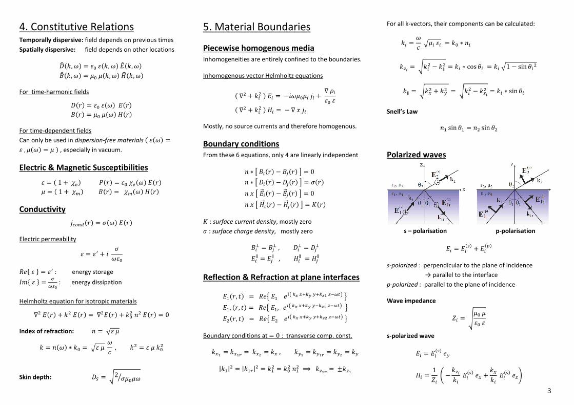
Polarized waves

s – polarisation p-polarisation

O{ = O{I�L + O{I�L

s-polarized : perpendicular to the plane of incidence

→ parallel to the interface

p-polarized : parallel to the plane of incidence

Wave impedance

ç{ = Ç|U |WU W

s-polarized wave

O{ = O{I�L �ª �{ = 1ç{ è − /«å/{ O{I�L �s + /s/{ O{I�L �«é

4

Fresnel Coefficients

T� = |�/«â − |. /«¡|� /«â + |. /«¡ T� = W� /«â − W. /«¡W� /«â + W. /«¡ K� = 2 |� /«â|� /«â + |. /«¡ K� = 2 W� /«âW�/«â + W. /«¡ Ç|� W.|. W�

They solve the two following equations:

O.I�L + O.ZI�L = O�I�L 1ç. è − /«â/. O.I�L + /«â/. O.ZI�L é = 1ç� è − /«¡/� é O�I�L

Total internal reflection: transmitted field evanescent

Total transmission

p-pol: Brewster angle : tan æ. = c¡câ W� /«â = W. /«¡ IT� = 0L s-pol: not possible, always partly reflected

Evanescent fields

O� = ì− O.I�L K� /«¡ / /�O.I�L K�O.I�L K� /s / /�í �{ ³ ¨» s¼¨À¡ « ´

/«â = /. Ð1 − sin� æ. , /«¡ = /� Ð1 − Yî� sin� æ.

Index of refraction: Yî = √tâ �â√t¡ �¡ = câc¡

Critical angle (afterwards evanescent/TIR): æ� = arcsin 1 Yî>

Frustrated total internal reflection Y� < Y- < Y.

vL æ. < vT��Y ^Y�Y._ ∶ �°Kℎ ±T°±. �L ��}¢: Y� �QvY. , Y- v0v�Y ±T°±. 2L æ. > vT��Y ^Y-Y._ ∶ �°Kℎ �QvY.

6. Energy and Momentum

Poynting’s Theorem

Explains the relation between electromagnetic fields and

their energy and therefore extends Maxwell’s equations.

Poynting vector: energy flux density, parallel to k-vector

¯ = O m �

Time average: ⟨ ¯ITL ⟩ = .� ¢�£ OITL m �∗ITL ¥

Far-field: ⟨ ¯ITL ⟩ = .� .òå |OITL|� ∗ YZ

Intensity }ITL = |È ¯ITL É| Density of electromagnetic energy

� = 12 N ~ ∗ O + R ∗ � S

Time-harmonic: � = .ó N ~ITL O∗ITL + RITL �∗ITL S

Total power : generated or dissipated inside the surface

�ô = h ⟨ ¯ITL ⟩ ∗ Y ]vwo = h }ITL ]vwo

Energy transport by evanescent waves

Dielectric interface; irradiated by plane wave under TIR

⟨¯⟩« = 12 ¢�º Os�ª∗ − Oª �s∗ Á = 0, � = ÇWUW|U| õ /jk/ m O ö ⟨¯⟩s = 12 ¢�º Oª �«∗ − O« �ª∗ Á ≠ 0 = 12 ÇW� |�W. |. sin æ. ^ |K�|� øO.I�Lø� + |K�|� ùO.I�Lù� _ ∗ �%�ú«

Maxwell stress tensor

Field momentum

ûü{*�w = 12� hN O m � S ]o

Time-averaged mechanical force

⟨�⟩ = h ⟨�ý IT, KL ⟩ ∗ YITL ]vwo

Maxwell’s stress tensor

þ�k = � WUW��+ |U| �� − 12 I WUWO� + |U|��L�ý �

Radiation pressure

Monochromatic plane wave, normal to interface

Part of the field is reflected at the material, superposed:

OIT, KL = O� ¢�£ N �{¨« + T ∗ �%{¨« S ∗ �%{¤  ¥ ∗ Ys �IT, KL = ÇWU|U OU ¢�£ N �{¨« − T ∗ �%{¨« S ∗ �%{¤  ¥ ∗ Yª

Radiation pressure

� Y« = �� Y« = 1� h⟨�ý IT, KL⟩ ∗ Y« ]vy

First two terms of stress tensor have no contribution, yield

� = }U2 N 1 + ¢S , }U = WU2 2 OU�

Reflectivity: ¢ = |T|� = 1 − � ¢ = 1: ±�T��2K�� T����2K;¢ = 0 ∶ Y°K

Perfectly reflecting material has twice

the radiation pressure of a non-reflecting

material

5

7. Radiation

Only accelerated charge can give rise to radiation.

The smallest radiating unit is a dipole, an electromagnetic

point source, and is used with the superposition principle.

Dyad: tensor of order two ( rank one )

Scalar and Vector potentials

OIT, KL = − ]]K �IT, KL − ∇ qIT, KL RIT, KL = ∇ m �IT, KL

� ∶ Q�2K°T ±°K�YK�v� , q ∶ �2v�vT ±°K�YK�v�

Dipole radiation

±IKL = MIKL ]� ]]K ±IKL = X] MIKL]K Y�` ]� = N fU ]vS ]� = fU ]

Current density of the elemental dipole

fIT, KL = ]]K ±IKL dI T − TU L

Vector potential of a time-harmonic dipole �IT, KL = ¢�£ �ITL �%{¤  ¥, qIT, KL = ¢�£ qITL �%{¤  ¥

N ∇� + /� S �ITL = −|U | fUITL N ∇� + /� S qITL = − 1WUW aUITL

Vector potential : �� J ��� �� � ���� �� J\ �ITL = −�¦|U| �{¨øZ%Z[ø4V |T − T\| ± = |U| h ûUIT, T\L fUIT\L ]′o

Scalar Green function

N ∇� + /� S ûUIT, T\L = dI T − T\ L

ûUIT, T\L = �{¨øZ%Z[ø4V |T − T\| Electric and magnetic dipole fields

OITL = ¦� |U | ûU�jjjk IT, T\L ± �ITL = −�¦ i ∇ m ûU�jjjk IT, T\L n ± = 1�¦|U I ∇ m O L

Dyadic Green function ( tensor )

ûU�jjjk IT, T\L = � }ý+ 1/� ∇ ∇ � ûUIT, T\L

In Cartesian coordinates: ¢ = |�| = |T − T\| ûU�jjjk IT, T\L = �{¨ 4V¢ X ^ 1 + �/¢ − 1/� ¢� _ �ý + 3 − 3�/¢ − /� ¢�/� ¢� � �¢� `

Near- , intermediate- and far-field

1. ¢ ≪ / → °Y�� K�T�� ²�Kℎ I /¢ L%- ��TQ�Q�

��jk�� = �{¨ 4V¢ 1/� ¢� � − �ý + 3 � �¢� �

2. ¢ ≈ / → °Y�� K�T�� ²�Kℎ I /¢ L%� ��TQ�Q�

��jk�� = �{¨ 4V¢ �/ ¢ � �ý − 3 � �¢� �

3. ¢ ≫ / → °Y�� K�T�� ²�Kℎ I /¢ L%. ��TQ�Q�

��jk�� = �{¨ 4V¢ � �ý − � �¢� �

Intermediate-field is 90° °�K °� ±ℎv�� in respect to the

near- and far-fied.

Non-vanishing field components in spherical coordinates

OZ = ± cos �4VWUW �{¨ZT /� � 2/�T� − 2�/T � O� = ± sin �4VWUW �{¨ZT /� � 1/�T� − �/T − 1 � �� = ± sin �4VWUW �{¨ZT /� � − �/T − 1� ÇWUW|U|

1. Far-field component is purely transverse

2. The near-field is dominated by the electric field

Radiation patterns and power dissipation

Radial component of the Poynting vector

⟨¯Z⟩ = 12 ¢� º O� ��∗ Á

With it, the resulting radiated power can be found by

�ô = h ��

U h | ⟨¯Z⟩ | T� sin � ]� ]��

U

Radiated power of a dipole

�ô = |±|�4VWUW Y- ¦ó3 2- = |±|� ¦ /-12 V WUW

In order to describe the radiation characteristic, we

calculate the power radiated at an infinitesimal unit solid

angle ] = sin � ]� ]� and normalize it:

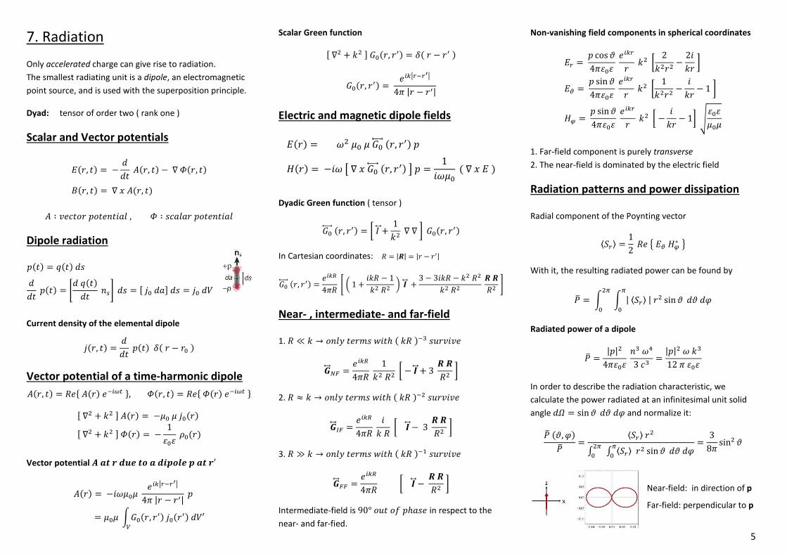
�ô I�, �L�ô = ⟨¯Z⟩ T�� ��U � ⟨¯Z⟩ T� sin � ]� ]��U = 38V sin� �

Near-field: in direction of p

Far-field: perpendicular to p

6

Dipole Radiation in arbitrary environments

Energy dissipation of dipole is influenced by surroundings.

�ô = ]�]K = − 12 h ¢� £ f∗ ∗ O ¥ ]o

By using the dipole’s current density ( TU: ]�±°�� °T�0�Y )

�ô = ¦2 }� £ ±∗ ∗ OITUL ¥ = ¦- |±|�2 2� WUW i Y� ∗ }�º ûý ITU, TUL Á ∗ Y� n

In an inhomogeneous surrounding, the field is a

superposition of the primary and scattered field:

OITUL = OUITUL + OÝITUL

Contribution of OU: �Uôôô = |�|¡.�� ¤tut /-

�ô�Uôôô = 1 + 6VWUW|±|� 1/- }�£ ±∗ ∗ OÝITUL ¥

Fields emitted by arbitrary sources

OITL = � ¦ |U | hûU�jjjk IT, T\L fIT\L ]\o �ITL = hi ∇ m ûU�jjjk IT, T\L n fIT′L ]\o

Sources with arbitrary time-dependence

Utilize Fourier transform: superposition of time harmonic

�IT, KL = |U4V |îIKL ∗ h ûUIT, T\, KL ∗ fU IT\, KL ]\Ã%Ã

ûUIT, T\, KL = 14V|T − T\| h �{¤ i  %cI¤LøZ%Z[ø �⁄ n ]¦Ã%Ã

Dispersion-free materials: YI¦L = Y , |I¦L = |

�IT, KL = |U|4V h fU IT\, K − |T − T\| Y 2⁄ L|T − T\| ]\o �IT, KL = 14VWUW h aU IT\, K − |T − T\| Y 2⁄ L|T − T\| ]\o

Dipole fields in time domain

Assume dipole in vacuum ( / = ¦ 2⁄ , W = 1 )

OZIKL = cos �4VWU � 2T- + 22T� ]]� � ±I�L | �   % Z� O�IKL = − sin �4VWU X 1T- + 12T� ]]� + 12�T ]�]��` ±I�L | �   % Z� ��IKL = − sin �4VWU ÇWU|U X 12T� ]]� + 12�T ]�]��` ±I�L | �   % Z� Far-field generated by acceleration of the dipole charges,

intermediate-field by velocity and near-field by position.

Lorentzian power spectrum

]�] ]¦ = 14VWU |±|� sin� � ¦U�4V� 2- !U� X !U� 4⁄I¦ − ¦UL� + !U� 4⁄ `

∆ ¦ = !U , !U ∶ ]v��Y0 2°Y�KvYK

Total radiated energy

� = |±|�4VWU¦Uó

3 2- !U

8. Angular Spectrum

OI" = 0, KL = �IKL → OI", KL = � #K − "2$

Series expansion of an arbitrary field in terms of plane

(and evanescent) waves with variable amplitudes and

propagation directions. For this, we we draw an arbitrary

axis " and consider the field E in a plane " = 2°Y�K. 2D Fourier transform ( /s , /ª are the spatial frequencies)

O ³/s, /ª; "´ = 14V� % OIm, �, "L �%{³¨» s¼¨½ ª´ ]m ]�Ã%Ã

OIm, �, "L = % O³/s, /ª ; "´ �{ ³¨» s¼¨½ ª´ ]/s ]/ªÃ

%Ã

/« = ·³ /� − /s� − /ª� ´ }�I/«L ≥ 0 , / = Ð|W ¦2

Evolution of the Fourier spectrum OÂ along the "-axis

O ³/s, /ª ; "´ = O ³ /s, /ª ; 0´ ∗ �± { ¨À «

+ : wave propagation in the half space " > 0

- : wave propagation in the half space " < 0

Angular Spectrum Representation

OIm, �, "L = % O ³/s, /ª ; 0´ ∗ �{ ³¨» s¼¨½ ª ± ¨À «´ ]/s ]/ªÃ

%Ã

�Im, �, "L = % �Ä ³/s, /ª; 0´ ∗ �{ ³¨» s¼¨½ ª ± ¨À «´ ]/s ]/ªÃ

%Ã

Express wave at any point by Fourier transform in " = 0

7

Using Maxwell: � = .{¤��u I ∇ m O L , ç�t = ·�u�tut

�Äs = 1 ç�t> i ³/ª /⁄ ´ O« − I/« /⁄ L Oª n

�Ī = 1 ç�t> i I/« /⁄ L OÂs − I/s /⁄ L O« n

�Ä« = 1 ç�t> i I/s /⁄ L Oª − ³/ª /⁄ ´ OÂs n

Divergence-free : / ∗ O = / ∗ �Ä = 0

Propagation and Focusing of Fields

Optical transfer function (OTF): �Ä ³/s, /ª ; "´ = �± { ¨À «

O ³/s , /ª ; "´ = �ij /s, /ª ; "´ O ³/s, /ª ; 0´

As linear response theory

Input : OÂ ³/s , /ª ; 0´

Filter function : �Ä ³/s, /ª ; "´

Output : OÂ ³/s , /ª ; "´

�Ä acts as a low-pass filter (only /s� + /ª� < /� can pass),

as evanescent waves are omitted. There is always a loss of

information from the near field to the far field.

Maximal resolution: ∆m ≈ .̈ = '��c

Calculation of the fields

OIm, �, "L = OIm, � ; 0L ∗ �Im, � ; "L

OI" = 2°Y�K. L = °YQ°��K�°Y I OI" = 0L, � L

�Im, �, "L = % �{ i ¨» s¼¨½ ª ± ¨À «n ]/s ]/ªÃ

%Ã

Paraxial Approximation

Wavevector / almost parallel to the "-axis I /s , /ª ≪ /L

/« = / ·1 − ³/s� + /ª�´//� ≈ / − ³ /s� + /ª� ´2 /

Gaussian Beams (does NOT fulfil Maxwell)

OIa, "L = OU ¦U¦I"L �% r¡¤¡I«L �{ i ¨∗« % (I«L ¼ ¨r¡ � I«L⁄ n

Where a = Ðm� + �� , "U = ¨ ¤u¡�

Beam radius: ¦I"L = ¦U I 1 + "� "U�⁄ Lâ¡

Wavefront radius: ¢I"L = " I1 + "U� "�⁄ L

Phase correction: ÕI"L = arctan "/"U

Transverse size: a , �° KℎvK ∶ |)Is,ª,«L||)IU,U,«L| = .*

Spaghetti formula

"U = / ¦U�2 , æ = 2/ ¦U

Numerical aperture (NA): �� ≈ 2Y//¦U

Rayleigh range *" : distance form the beam waist to where

the beam radius has increased by a factor of √2

Beam stays roughly focused over a distance of # *".

Gouy phase shift: 180° shift from " → −∞ K° " → ∞

Far-field Approximation

� = ³ �s , �ª , �« ´ = # mT , �T , "T $ = è /s/ , /ª/ , /«/ é

Evanescent waves vanish. Now only ³ /s� + /ª� ´ < /

Oó�s, �ª´ = −2V� / �« O³ /�s, /�ª ;0´ �{¨ZT

with �« = ·1 − ³ �s� + �ª� ´ = " T⁄

Far-field entirely defined by Fourier spectrum at " = 0.

Only one plane wave with wave vector / of the angular

spectrum at " = 0 contributes to the far-field in � direction.

The rest gets cancelled by destructive interference.

Therefore, the far-field behaves as a collection of rays

where each ray is characterized by a particular plane wave

of the original angular spectrum representation.

OÂ ³/s, /ª ;0´ = � T �% {¨Z2V /« OÃ è /s/ , /ª/ é

OIm, �, "L = { Z *, å-ã�� % Oà # ¨»̈ , ¨½̈ $³¨»¡ ¼ ¨½¡´ . ¨¡ … … �{ i ¨» s ¼ ¨½ ª ± ¨À « n 1/« ]/s ]/ª

O vY] Oà �°T� v �°�T��T KTvY��°T� ±v�T vK " = 0 �°T Kℎ� v±±T°m��vK�°Y /« ≈ /, Kℎ�� ±v�T �� ±�T��2K. Object plane: " = 0

Image plane: " = "U I�vT ����]: "U → ∞ L

Fourier optics: /« ≈ / , R only dependent on z

8

Fresnel & Fraunhofer diffraction

T� = Im − m\L� + I� − �\L� + "� = ¢� X 1 − 2Imm\ − ��\L¢� + m\� + �\�¢� `

Determine the field at the observation point using Huygens

principle of “summing up” elementary spherical waves:

h �Im\, �\L �% { ¨ Z³s[,ª[´TIm\, �\L ]m\ ]�\« U

We can set TIm\, �\L ≈ ¢ in the denominator due to the

large distance between source and observer. However, we

cannot neglect interference effects in the exponent.

With the paraxial approximation, we get:

Maximum extend of the source at " = 0

~ 2⁄ = �vm 0 ·m\� + �\� 1

For "U ≫ ~ , we can use Fraunhofer. Else, we use Fresnel.

The transition between Fraunhofer and Fresnel happens

around the Rayleigh range "U

"U = 1 8> / ~� , ¦U = ~ 2>

The Point-Spread function

Measure of the resolving power of an imaging system: the

narrower the function, the better the resolution.

Due to the loss of evanescent waves (with their high

spatial frequencies) and the finite angular collection, the

point appears as a function with finite width.

Magnification: � = Y. Y�> ∗ �� �.>

Numerical aperture: �� = Y. sinI�vmNæ.SL = �� �.> sinI�vmNæ�SL

Airy disk radius: ∆m = 0.6098 2 '�y

9. Waveguides & Resonators

Resonators confine electromagnetic energy

Waveguides guide this electromagnetic energy

9.1 Resonators

Consider a rectangular box with sides Ës , ˪ , Ë«

We now search solutions for Helmholtz: N ∇� + /�S O = 0

1. Ansatz: OsIm, �, "L = OUIsL 3ImL 4I�L çI"L ;Oª = …

2. Separation of variables 13

]�3] m� + 14

]�4] �� + 1ç ]�ç] "� + /� = 0

3. Set constants to − /s�, −/ª�, −/«� , which implies

/s� + /ª� + /«� = /� = ¦�2� Y�I¦L

4. We obtain tree separate equations ]�3]m� + /s� 3 = ]�4]�� + /ª� 4 = ]�ç]"� + /«� ç = 0

5. → OsIm, �, "L = OUIsLi2.,s �% {¨»s + 2�,s �{¨»sn… … i2-,s �% {¨½ª + 2ó,s �{¨½ªni25,s �% {¨À« + 26,s �{¨À«n 6.Boundary conditions:

OsI� = 0L = Os³� = ˪´ = 0 = OsI" = 0L = OsI" = Ë«L

7. Use ∇ ∗ O = 0 , I ∇ ∗ � = 0, ∇ m O = 0 L

OsIm, �, "L = OUIsL cos �Y V mËs� sin X � V �˪` sin � � V "Ë«� OªIm, �, "L = OUIªL sin �Y V mËs� cos X � V �˪` sin � � V "Ë«� O«Im, �, "L = OUI«L sin �Y V mËs� sin X � V �˪` cos � � V "Ë«�

9

YËs OU

(s) + �˪ OU

(ª) + �Ë«

OU(«) = 0

Dispersion relation / mode structure of the resonator

V� X Y�Ës� + ��˪� + ��Ë«� ` = ¦c���2� Y�I¦c��L , Y, �, � ∈ ℤU

Density of States (DOS)

Finite-size box with equal length: Ë = Ës = ˪ = Ë«

→ Y� + �� + �� = � ËV ∗ ¦c��2 YI¦c��L��

If Y, �, � ∈ ℝ ∶ TU = N ¦c��Ë YI¦c��L IV2L⁄ S

The number of different modes in interval N ¦…¦ + ∆¦S

]�I¦L]¦ ∆¦ = ¦� Y-I¦LV� 2- ∆¦

States that there are more modes for higher frequencies.

Density of States (DOS)

aI¦L = ¦� Y-I¦LV� 2-

DOS: number of modes per unit volume V and unit frequency ∆¦

Number of modes

�I¦L = h o h aI¦L ]¦ ]¤¡¤â

Example: Power emitted by a dipole

�ô = V ¦�12 WU W |±|� aI¦L

Quality factor

Due to losses such as absorption and radiation, the

discrete frequencies broaden to a finit line width ∆¦ = 2! x = ¦U/!

Measure for how long energy can be stored in a resonator

Due to the losses, the electric field diminishes:

OIT, KL = ¢�£ OUITL exp � ^�¦U − ¦U2x_ K�

Where ¦U is one of the resonant frequencies ¦c�� .

Spectrum of the stored energy density

�¤I¦L = ¦U�4x� �¤I¦ULI¦ − ¦UL� + I¦U 2x⁄ L�

Cavity Perturbance (Disturbance theory of a resonator)

Particle absorption or a change of the index of refraction

can lead to a shift of the resonance frequency

Unperturbed system (¦U ∶ T��°YvY2� �T�M��Y2�)

∇ m OU = �¦U|U|ITL �U , ∇ m �U = − �¦UWUWITL OU

Perturbed system ( ∆W, ∆| ∶ �vK�T�v� ±vTv� °� ±vTK�2��)

∇ m O = �¦|U N |ITL � + ∆|ITL � S ∇ m � = − �¦WU N WITL O + ∆WITL O S

Bethe-Schwinger cavity perturbation formula ¦ − ¦U¦ = − � N OU∗ WU ∆WITL O + �U∗ |U ∆|ITL � S ]∆o � N WU WITL OU∗ O + |U |ITL �U∗ � S ]o Assuming a small effect of the perturbation on the cavity: O = OU, � = �U

¦ − ¦U¦ = − � N OU∗ WU ∆WITL OU + �U∗ |U ∆|ITL �U S ]∆o � N WU WITL OU∗ OU + |U |ITL �U∗ �U S ]o For a weakly-dispersive medium: ¦ − ¦U¦ = − ∆��U ⇔ ¦ = ¦U � �U�U − ∆� �

Waveguides

Used to carry electromagnetic energy from A to B

Parallel-Plate waveguides

Material with YI¦L sandwiched between two conductors

TE-Mode: no electric field in propagation direction

TM-Mode: no magnetic field in propagation direction

TE-Modes: electric field parallel to surfaces of the plates

Ansatz: plane wave propag. at angle æ to surface normal

O.Im, �, "L = OU Yª �N %{¨s <=�>¼{¨« �ÌÍ> S Coming from the upper plate, it gets reflected at the bottom: O�Im, �, "L = − OU Yª �N {¨s <=�>¼{¨« �ÌÍ> S Superposition of the fields:

OIm, �, "L = O. + O� = −2� OU Yª �{ ¨ « �{c> sinI/ m cos æL

Quantisation of the normal wavenumber: field must fulfil

boundary condition at the upper plate: OIm, �, ]L = 0

sinN /] cos æ S = 0 → /] cos æ = Y V /s = / cos æ → /s? = Y V ]> , Y ∈ £1,2,… ¥

As /� = /s� + /«� , we can find the propagation constant

/«? = ·/� − /s?� = Ð/� − Y�NV ]⁄ S� , Y ∈ £ 1,2,… ¥

Y = 0 : zero-field (trivial solution for TE-modes) c �w > / : exponential decay just like evanescent waves

→ High-pass filter

10

Cut-off frequency

¦� = Y V 2] YI¦�L , Y ∈ £ 1, 2,… ¥

Below the cut-off frequency, waves cannot propagate

¦ > ¦� ∶ �ℎv�� Q��°2�K� Q�@ = ¦ /«? ⁄ ûT°�± Q��°2�K� Q� = ]¦ ]/«? ⁄

TM-Modes: magnetic field parallel to surfaces of plates

Ansatz: plane wave propag. at angle æ to surface normal

�.Im, �, "L = �U Yª �N %{¨s <=�>¼{¨« �ÌÍ> S Coming from the upper plate, it gets reflected at the bottom: ��Im, �, "L = �U Yª �N {¨s <=�>¼{¨« �ÌÍ> S Superposition of the fields:

�Im, �, "L = �. + �� = 2 �U Yª �{ ¨ « �{c> cosI/ m cos æL

Boundary condition at top interface " = ] leads to

/] cos æ = YV , Y ∈ £ 0, 1, 2,… ¥

/«? = Ð/� − Y� NV ]⁄ S� , Y ∈ £ 0, 1, 2,… ¥

TEM / ��UU – Mode

In contrast to the TE-modes, there exists a mode for Y = 0.

This mode does NOT have a cut-off frequency like all other

TM- and TE-modes.

For ��UU ∶ /« = /

This is a transverse electric field: neither the electric nor

the magnetic field show in the direction of propagation.

Hollow Metal Waveguides

Ansatz: OIm, �, "L = OsªIm, �L ∗ �{¨À «

O = O Z�c�A + O��c� = O m Y« + I O ∗ Y«L Y«

The transverse field components can be calculated using

the longitudinal field components:

TE-Modes: O«sª = 0

�«sªI2, mL = �UÀ cos B c�C» mD cos � ��C½ � � , Y, � ∈ £0,1,… ¥

Transverse wavenumber:

/ � = i /s� + /ª� n = V� X Y�Ës� + ��˪� ` , Y, � ∈ £0, 1,… ¥

Frequency of the �Oc� modes:

¦c� = V2YI¦c�L ÇY�Ës� + ��˪� , Y, � ∈ £0,1,… ¥

Watch out: �OUU does not exist! Therefore, Y = 0 = � is

not a valid solution; the lowest frequency modes are hence �OU. vY] �O.U .

Propagation constant / longitudinal wavenumber

/« = ·/� − / � = Ǧc��2� Y�I¦c�L − X Y�V�Ës� + ��V�˪� `

As there is no zero mode, there is always a cut-off.

TM-Modes : �«sª = 0

O«sªIm, �L = OUÀ sin � YVËs m � sin X �V˪ � ` , Y, � ∈ £ 1,… ¥

Y = 0 °T � = 0 lead to zero-field solutions and are

forbidden. The lowest frequency mode is ��...

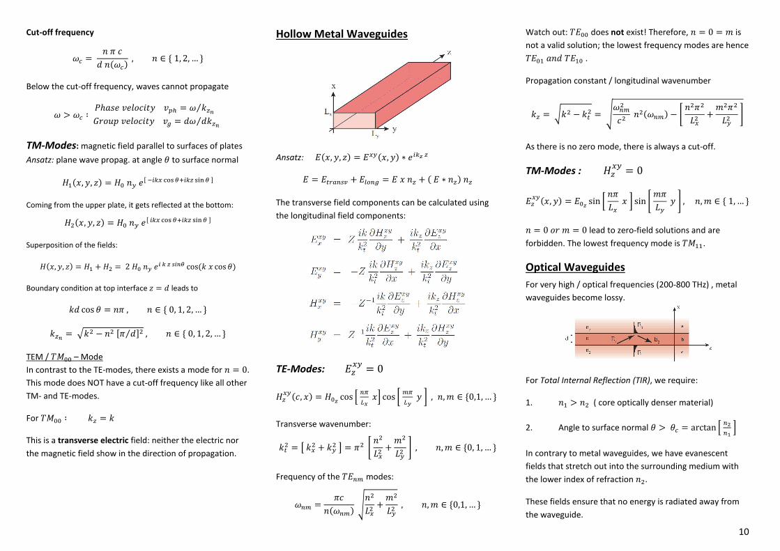
Optical Waveguides

For very high / optical frequencies (200-800 THz) , metal

waveguides become lossy.

For Total Internal Reflection (TIR), we require:

1. Y. > Y� ( core optically denser material)

2. Angle to surface normal æ > æ� = arctan B c¡câ D In contrary to metal waveguides, we have evanescent

fields that stretch out into the surrounding medium with

the lower index of refraction Y�.

These fields ensure that no energy is radiated away from

the waveguide.

11

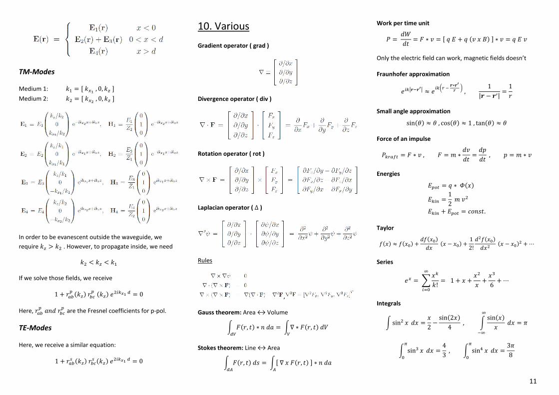
TM-Modes

Medium 1: /. = N /sâ , 0, /« S

Medium 2: /� = N /s¡ , 0, /« S

In order to be evanescent outside the waveguide, we

require /« > /� . However, to propagate inside, we need

/� < /« < /.

If we solve those fields, we receive

1 + T�E� I/«L TE�� I/«L ��{¨»â w = 0

Here, T�E� vY] TE�� are the Fresnel coefficients for p-pol.

TE-Modes

Here, we receive a similar equation:

1 + T�E� I/«L TE�� I/«L ��{¨»â w = 0

10. Various

Gradient operator ( grad )

Divergence operator ( div )

Rotation operator ( rot )

Laplacian operator ( ∆ )

Rules

,

Gauss theorem: Area ↔ Volume

h �IT, KL ∗ Y ]vwo = h∇ ∗ �IT, KL ]o

Stokes theorem: Line ↔ Area

h �IT, KL ]�wy = hN ∇ m �IT, KL S ∗ Y ]vy

Work per time unit

� = ]�]K = � ∗ Q = N M O + M IQ m RL S ∗ Q = M O Q

Only the electric field can work, magnetic fields doesn’t

Fraunhofer approximation

�{¨øJ%J[ø ≈ �{¨^Z % J∗J[Z _ , 1|J − J\| = 1T

Small angle approximation sinIæL ≈ æ , cosIæL ≈ 1 , tanIæL ≈ æ

Force of an impulse

�̈ Z�ü  = � ∗ Q , � = � ∗ ]Q]K = ]±]K , ± = � ∗ Q

Energies O��  = M ∗ qImL O¨{c = 12 � Q� O¨{c + O��  = 2°Y�K. Taylor

�ImL ≈ �ImUL + ]�ImUL]m Im − mUL + 12!]��ImUL]m� Im − mUL� +⋯

Series

�s = H m¨/!Ã

{ U = 1 + m + m�m + m-6 +⋯

Integrals

h sin� m ]m = m2 − sinI2mL4 , h sinImLm ]mÃ%Ã = V

h sin- m ]m�U = 4

3 , h sinó m ]m�U = 3V8

12

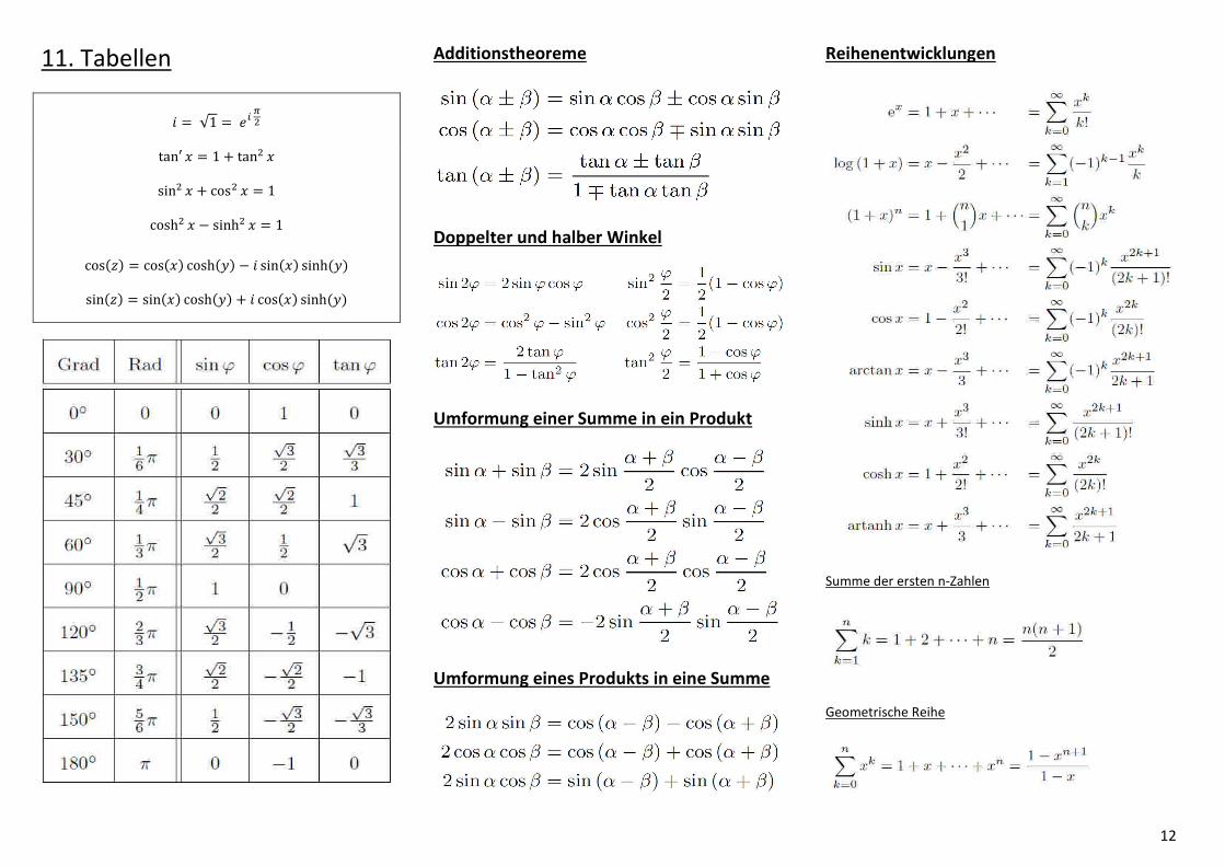
11. Tabellen

� = √1 = �{ ��

tan′ m = 1 + tan� m

sin� m + cos� m = 1

cosh� m − sinh� m = 1 cosI"L = cosImL coshI�L − � sinImL sinh I�L

sinI"L = sinImL coshI�L + � cosImL sinh I�L

Additionstheoreme

Doppelter und halber Winkel

Umformung einer Summe in ein Produkt

Umformung eines Produkts in eine Summe

Reihenentwicklungen

Summe der ersten n-Zahlen

Geometrische Reihe

13

Fourier-Korrespondenzen

Eigenschaften der Fourier-Transformation

Partialbruchzerlegung (PBZ)

Reelle Nullstellen n-ter Ordnung:

�.(m − v¨) + ��Im − v¨)� + …+ �cIm − v¨)c

Paar komplexer Nullstellen n-ter Ordnung:

R.m + .(m − v¨)(m − v¨) + …+ Rcm + c

N(m − v¨)(m − v¨)Sc +

(m − v¨)(m − v¨) = Im − ¢�L� + }��

Fourier-Tabelle

Fourier-Funktionen

14

Ableitungen

Stammfunktionen

Standard-Substitutionen

15

16