EFFICIENT SURFACE-AWARE SEMI-GLOBAL MATCHING WITH MULTI-VIEWPLANE-SWEEP SAMPLING

B. Rufa,b, T. Polloka, M. Weinmannb

aFraunhofer IOSB, Video Exploitation Systems, Karlsruhe, Germany -{boitumelo.ruf, thomas.pollok}@iosb.fraunhofer.de

bInstitute of Photogrammetry and Remote Sensing, Karlsruhe Institute of Technology,Karlsruhe, Germany - {boitumelo.ruf, martin.weinmann}@kit.edu

Commission II, WG II/4

KEY WORDS: Depth Estimation, Normal Map Estimation, Semi-Global-Matching, Multi-View, Plane-Sweep Stereo, Online Pro-cessing, Oblique Aerial Imagery

ABSTRACT:

Online augmentation of an oblique aerial image sequence with structural information is an essential aspect in the process of 3D sceneinterpretation and analysis. One key aspect in this is the efficient dense image matching and depth estimation. Here, the Semi-GlobalMatching (SGM) approach has proven to be one of the most widely used algorithms for efficient depth estimation, providing a goodtrade-off between accuracy and computational complexity. However, SGM only models a first-order smoothness assumption, thusfavoring fronto-parallel surfaces. In this work, we present a hierarchical algorithm that allows for efficient depth and normal mapestimation together with confidence measures for each estimate. Our algorithm relies on a plane-sweep multi-image matching followedby an extended SGM optimization that allows to incorporate local surface orientations, thus achieving more consistent and accurateestimates in areas made up of slanted surfaces, inherent to oblique aerial imagery. We evaluate numerous configurations of our algorithmon two different datasets using an absolute and relative accuracy measure. In our evaluation, we show that the results of our approachare comparable to the ones achieved by refined Structure-from-Motion (SfM) pipelines, such as COLMAP, which are designed foroffline processing. In contrast, however, our approach only considers a confined image bundle of an input sequence, thus allowing toperform an online and incremental computation at 1Hz−2Hz.

1. INTRODUCTION

Dense image matching is one of the most important and inten-sively studied task in photogrammetric computer vision. It allowsto estimate dense depth maps which, in turn, alleviate the pro-cesses of dense 3D reconstruction and model generation (Blaha etal., 2016; Bulatov et al., 2011; Musialski et al., 2013; Rothermelet al., 2014), navigation of autonomous vehicles such as robots,cars and unmanned aerial vehicles (UAVs) (Barry et al., 2015;Menze and Geiger, 2015; Scaramuzza et al., 2014), as well asscene interpretation and analysis (Taneja et al., 2015; Weinmann,2016). Especially in combination with small commercial off-the-shelf (COTS) UAVs it allows for a cost-effective monitoring ofman-made structures from aerial viewpoints.

In general, dense image matching algorithms can be grouped intotwo categories, namely local and global methods (Scharstein andSzeliski, 2002). Since local methods only consider a confinedneighborhood by aggregating a matching cost in a local aggre-gation window, they can be computed very efficiently, allowingto achieve real-time processing. However, their smoothness as-sumptions are restricted to the local support region and thereforethe accuracies achieved by these methods are typically not in theorder of those achieved by global methods.

First introduced by Hirschmueller (2005, 2008), Semi-GlobalMatching (SGM) combines the benefits of both local and globalmethods. The use of dynamic programming to approximate theenergy minimization, by independently aggregating along numer-ous concentric one-dimensional paths, provides a good trade-off

between accuracy and computational complexity. Thus, SGM isstill one of the most widely used algorithms for efficient image-based depth estimation from both two-view and multiple-viewsetups. Furthermore, recent studies show that the SGM algo-rithm can be adapted to allow for real-time stereo depth estima-tion solely on a desktop CPU (Gehrig and Rabe, 2010; Spangen-berg et al., 2014) or embedded hardware (Banz et al., 2011; Hof-mann et al., 2016; Ruf et al., 2018a).

However, SGM only models a first-order smoothness assumption,thus favoring fronto-parallel surfaces. This is sufficient for appli-cations, in which the existence of a reconstructed 3D object ismore important than its detailed appearance, such as robot nav-igation. Nonetheless, when it comes to a visually accurate 3Dreconstruction of slanted surfaces, which are inherent to obliqueaerial imagery, a second-order smoothness assumption is desir-able. To overcome this restriction, Scharstein et al. (2017) pro-pose to incorporate priors, such as normal maps, to dynamicallyadjust SGM to the surface orientation of the object that is to bereconstructed.

In this work, we propose an algorithm that extends SGM to amulti-image matching, which allows for online augmentation ofan aerial image sequence with structural information and focuseson oblique imagery captured from small UAVs. Thus, our contri-bution is an approach for image-based depth estimation, that

• relies on a hierarchical multi-image semi-global stereomatching,

arX

iv:1

909.

0989

1v1

[cs

.CV

] 2

1 Se

p 20

19

• favors not only fronto-parallel surfaces but incorporates aregularization based on local surface normals, and

• allows for efficient depth and normal map estimation withconfidence measures from aerial imagery.

This paper is structured as follows: In Section 2, we briefly sum-marize the related work on algorithms that rely on SGM and al-low for efficient image-based depth estimation. We specificallyfocus on the use of non-fronto-parallel smoothness assumptionsallowing for slanted surface reconstruction. In Section 3, we givea detailed overview on our methodology, focusing on our adap-tation of SGM to be used with multi-image matching for densedepth estimation from oblique aerial imagery, together with theestimation of surface normals and confidence measures. We eval-uate our approach on two datasets (Section 4) and present ourachieved results in Section 4.1, which is followed by a discussionin Section 4.2. Finally, we provide a summary, concluding re-marks, and a short outlook on future improvements in Section 5.

2. RELATED WORK

In recent years, a number of software suites to address accu-rate dense 3D reconstruction have been released. These includethe Structure-from-Motion (SfM) pipelines SURE (Rothermel etal., 2012; Wenzel et al., 2013) and COLMAP (Schonberger andFrahm, 2016; Schonberger et al., 2016), that enable the creationof detailed 3D models from a large set of input images. While thefocus of these pipelines lies on the accuracy and completeness ofthe resulting 3D model, they are designed for offline processing,in which computation time is not a critical factor and all input im-ages are available at the time of reconstruction. However, sinceour work focuses on online processing, computation time is acritical factor for us and we cannot assume that the complete in-put sequence is available for the process of 3D reconstruction. Inaddition, since we aim at methods that generate a dense field ofdepth estimates, we use a direct dense image matching for thecomputation of depth maps, instead of sparse feature matching.

When it comes to efficient dense image matching, the Semi-Global Matching (SGM) algorithm (Hirschmueller, 2005, 2008)has evolved to a suitable and widely used approach. The accu-racy achieved with respect to the computation time needed makesSGM very appealing for both offline and online processing. Intheir work, Spangenberg et al. (2014) as well as Gehrig and Rabe(2010) show that, when using a fixed stereo setup, SGM can beoptimized to run at 16 fps and 14 fps, respectively, on a conven-tional desktop CPU when utilizing SIMD instructions and usinginput images at VGA resolution. The most common optimiza-tion strategy for the SGM algorithm, however, is to utilize themassively parallel computation infrastructure of modern GPUs,achieving real-time frame rates (Banz et al., 2011). An alterna-tive is to allow for dense image matching from aerial imagerywith large disparities by encapsulating the SGM approach in ahierarchical processing scheme (Rothermel et al., 2012; Wenzelet al., 2013). Even in the field of embedded stereo processing,real-time performance with high accuracies can be achieved byoptimizing the SGM approach for FPGA architectures (Barry etal., 2015; Hofmann et al., 2016; Ruf et al., 2018a).

In more recent work, Scharstein et al. (2017) have proposed animprovement to the accuracy of the SGM approach by includingavailable surface priors to better cope with slanted surfaces anduntextured regions. Similarly, Hermann et al. (2009) and Ni et al.

(2018) propose to extend SGM by incorporating a second-ordersmoothness assumption, that also allows to favor non-fronto-parallel surfaces.

The so-called plane-sweep sampling for true multi-image match-ing was first introduced by Collins (1996) and was adopted in agreat amount of studies aiming at real-time depth estimation and3D reconstruction from image sequences. Among many are thework of Gallup et al. (2007) and Sinha et al. (2014). Gallup etal. (2007) introduced an extension to the plane-sweep algorithmthat does not only consider a fronto-parallel sweeping directionbut also incorporates other plane orientations that align with thescene geometry, e.g. ground plane. Sinha et al. (2014) furtherextend the plane-sweep approach for multi-image matching byidentifying different plane configurations for local image regionsin contrast to using the same plane orientations for the whole im-age. Furthermore, Sinha et al. (2014) also propose to use thesemi-global optimization strategy to extract the final disparity im-age from the result of the local plane-sweep sampling.

In our work, we incorporate and evaluate the strengths of multi-ple approaches by using a hierarchical multi-view image match-ing and considering surface normals to better handle non-fronto-parallel surfaces in the semi-global optimization scheme.

3. METHODOLOGY

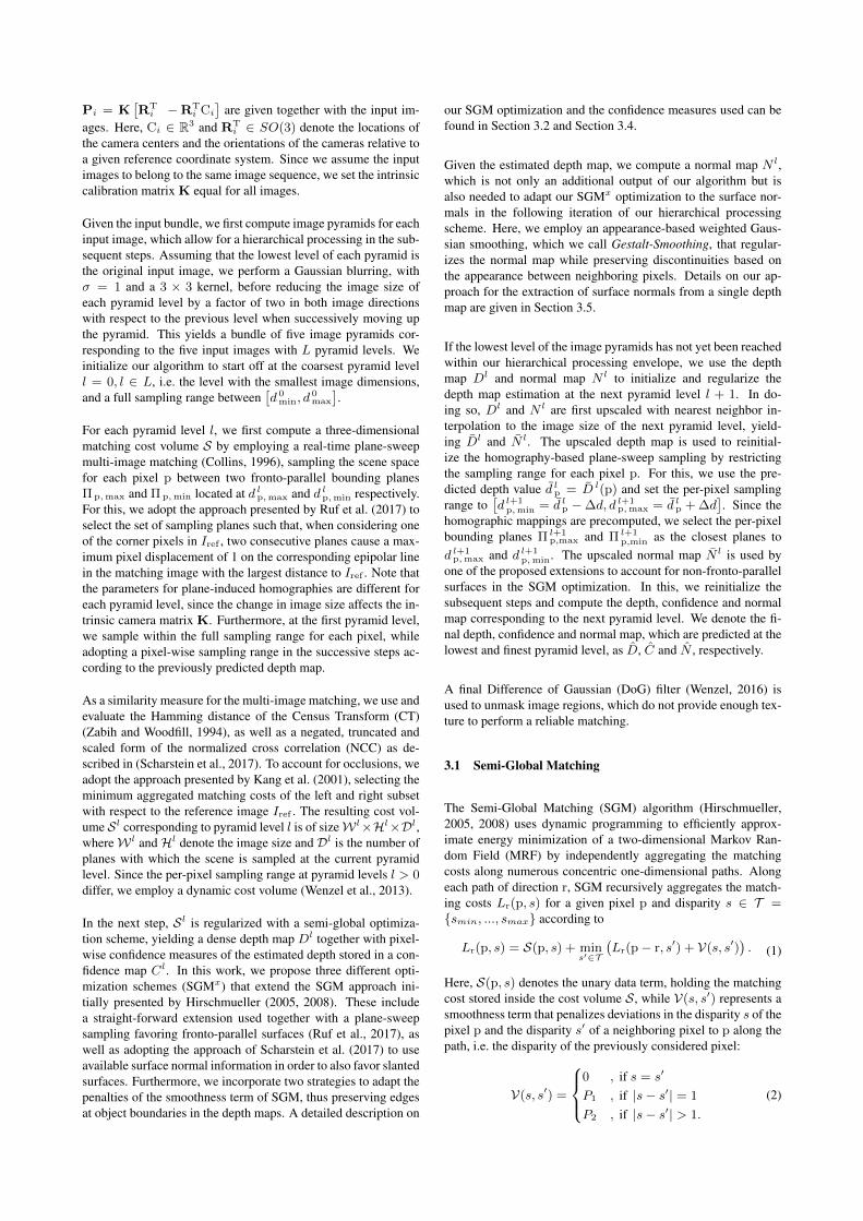
Figure 1 depicts the processing pipeline of our approach for ahierarchical multi-image matching followed by a surface-awareand edge-preserving SGM optimization together with a compu-tation of surface normals and confidence measures. We first givea brief overview on all processing steps before we provide a de-tailed description of our extensions of the SGM algorithm, thecomputation of confidence measures, as well as a detailed expla-nation on the computation of surface normals.

Ii,Pi

Image pyramid generation

Depth map estimation

Plane-sweep sampling

SGMx optimization

Normal map estimation

Sampling range computation

Upscaling

l = 0, [d 0min, d

0max]

Dl, C l

Dl, C l, N l

D, C, N

l ==lowestpyr.lvl.

Dl, N l

N l,[d l+1

p,min, dl+1p,max

]

Figure 1. Overview of the proposed methodology. Given five images Iiof an input sequence, we perform hierarchical SfM to estimate a depth,confidence and normal map (D, C, N).

As input to our processing pipeline, we choose a bundle of fiveimages Ii of an input sequence which depict the scene that isto be reconstructed from five slightly different viewpoints. Weselect the center image of the input bundle as reference imageIref for which the depth, normal and confidence maps are tobe computed. To this end, we assume that the camera poses

Pi = K[RT

i −RTi Ci

]are given together with the input im-

ages. Here, Ci ∈ R3 and RTi ∈ SO(3) denote the locations of

the camera centers and the orientations of the cameras relative toa given reference coordinate system. Since we assume the inputimages to belong to the same image sequence, we set the intrinsiccalibration matrix K equal for all images.

Given the input bundle, we first compute image pyramids for eachinput image, which allow for a hierarchical processing in the sub-sequent steps. Assuming that the lowest level of each pyramid isthe original input image, we perform a Gaussian blurring, withσ = 1 and a 3 × 3 kernel, before reducing the image size ofeach pyramid level by a factor of two in both image directionswith respect to the previous level when successively moving upthe pyramid. This yields a bundle of five image pyramids cor-responding to the five input images with L pyramid levels. Weinitialize our algorithm to start off at the coarsest pyramid levell = 0, l ∈ L, i.e. the level with the smallest image dimensions,and a full sampling range between

[d 0

min, d0max

].

For each pyramid level l, we first compute a three-dimensionalmatching cost volume S by employing a real-time plane-sweepmulti-image matching (Collins, 1996), sampling the scene spacefor each pixel p between two fronto-parallel bounding planesΠ p, max and Π p,min located at d l

p,max and d lp,min respectively.

For this, we adopt the approach presented by Ruf et al. (2017) toselect the set of sampling planes such that, when considering oneof the corner pixels in Iref , two consecutive planes cause a max-imum pixel displacement of 1 on the corresponding epipolar linein the matching image with the largest distance to Iref . Note thatthe parameters for plane-induced homographies are different foreach pyramid level, since the change in image size affects the in-trinsic camera matrix K. Furthermore, at the first pyramid level,we sample within the full sampling range for each pixel, whileadopting a pixel-wise sampling range in the successive steps ac-cording to the previously predicted depth map.

As a similarity measure for the multi-image matching, we use andevaluate the Hamming distance of the Census Transform (CT)(Zabih and Woodfill, 1994), as well as a negated, truncated andscaled form of the normalized cross correlation (NCC) as de-scribed in (Scharstein et al., 2017). To account for occlusions, weadopt the approach presented by Kang et al. (2001), selecting theminimum aggregated matching costs of the left and right subsetwith respect to the reference image Iref . The resulting cost vol-ume Sl corresponding to pyramid level l is of sizeW l×Hl×Dl,whereW l andHl denote the image size and Dl is the number ofplanes with which the scene is sampled at the current pyramidlevel. Since the per-pixel sampling range at pyramid levels l > 0differ, we employ a dynamic cost volume (Wenzel et al., 2013).

In the next step, Sl is regularized with a semi-global optimiza-tion scheme, yielding a dense depth map Dl together with pixel-wise confidence measures of the estimated depth stored in a con-fidence map Cl. In this work, we propose three different opti-mization schemes (SGMx) that extend the SGM approach ini-tially presented by Hirschmueller (2005, 2008). These includea straight-forward extension used together with a plane-sweepsampling favoring fronto-parallel surfaces (Ruf et al., 2017), aswell as adopting the approach of Scharstein et al. (2017) to useavailable surface normal information in order to also favor slantedsurfaces. Furthermore, we incorporate two strategies to adapt thepenalties of the smoothness term of SGM, thus preserving edgesat object boundaries in the depth maps. A detailed description on

our SGM optimization and the confidence measures used can befound in Section 3.2 and Section 3.4.

Given the estimated depth map, we compute a normal map N l,which is not only an additional output of our algorithm but isalso needed to adapt our SGMx optimization to the surface nor-mals in the following iteration of our hierarchical processingscheme. Here, we employ an appearance-based weighted Gaus-sian smoothing, which we call Gestalt-Smoothing, that regular-izes the normal map while preserving discontinuities based onthe appearance between neighboring pixels. Details on our ap-proach for the extraction of surface normals from a single depthmap are given in Section 3.5.

If the lowest level of the image pyramids has not yet been reachedwithin our hierarchical processing envelope, we use the depthmap Dl and normal map N l to initialize and regularize thedepth map estimation at the next pyramid level l + 1. In do-ing so, Dl and N l are first upscaled with nearest neighbor in-terpolation to the image size of the next pyramid level, yield-ing Dl and N l. The upscaled depth map is used to reinitial-ize the homography-based plane-sweep sampling by restrictingthe sampling range for each pixel p. For this, we use the pre-dicted depth value d l

p = D l(p) and set the per-pixel samplingrange to

[d l+1

p,min = d lp −∆d, d l+1

p,max = d lp + ∆d

]. Since the

homographic mappings are precomputed, we select the per-pixelbounding planes Π l+1

p,max and Π l+1p,min as the closest planes to

d l+1p,max and d l+1

p,min. The upscaled normal map N l is used byone of the proposed extensions to account for non-fronto-parallelsurfaces in the SGM optimization. In this, we reinitialize thesubsequent steps and compute the depth, confidence and normalmap corresponding to the next pyramid level. We denote the fi-nal depth, confidence and normal map, which are predicted at thelowest and finest pyramid level, as D, C and N , respectively.

A final Difference of Gaussian (DoG) filter (Wenzel, 2016) isused to unmask image regions, which do not provide enough tex-ture to perform a reliable matching.

3.1 Semi-Global Matching

The Semi-Global Matching (SGM) algorithm (Hirschmueller,2005, 2008) uses dynamic programming to efficiently approx-imate energy minimization of a two-dimensional Markov Ran-dom Field (MRF) by independently aggregating the matchingcosts along numerous concentric one-dimensional paths. Alongeach path of direction r, SGM recursively aggregates the match-ing costs Lr(p, s) for a given pixel p and disparity s ∈ T ={smin, ..., smax} according to

Lr(p, s) = S(p, s) + mins′∈T

(Lr(p− r, s′) + V(s, s′)

). (1)

Here, S(p, s) denotes the unary data term, holding the matchingcost stored inside the cost volume S, while V(s, s′) represents asmoothness term that penalizes deviations in the disparity s of thepixel p and the disparity s′ of a neighboring pixel to p along thepath, i.e. the disparity of the previously considered pixel:

V(s, s′) =

0 , if s = s′

P1 , if |s− s′| = 1

P2 , if |s− s′| > 1.

(2)

At each pixel, the individual path costs are summed up, resultingin an aggregated cost volume

S(p, s) =∑r

Lr(p, s) (3)

from which the pixel-wise winning disparities are extracted ac-cording to

S(p) = arg minsS(p, s). (4)

3.2 Extensions of the Semi-Global Matching Algorithm(SGMx)

The first of the proposed SGMx extensions, which at the sametime serves as a basis to the other two extensions, is a straight-forward adaptation of the standard SGM approach to the use ofa fronto-parallel multi-view plane-sweep sampling as part of thework flow presented in Figure 1. It is thus denoted as fronto-parallel SGM (SGMfp) and was already used in (Ruf et al., 2017)and (Ruf et al., 2018b). The recursive aggregation of the match-ing costs along each path is adjusted to

Lr(p,Πd) = S(p,Πd) +

mind′∈D

(Lr(p− r,Πd′) + Vfp(Πd,Πd′)) ,(5)

with Πd being the sampling plane at depth d used to performthe multi-image matching. Here, instead of penalizing the devia-tions in neighboring disparities, the smoothness term Vfp penal-izes different planes between adjacent pixels along the path Lr:

Vfp(Πd,Πd′) =

0 , if Γ(Πd) = Γ(Πd′)

P1 , if |Γ(Πd)− Γ(Πd′)| = 1

P2 , if |Γ(Πd)− Γ(Πd′)| > 1,

(6)

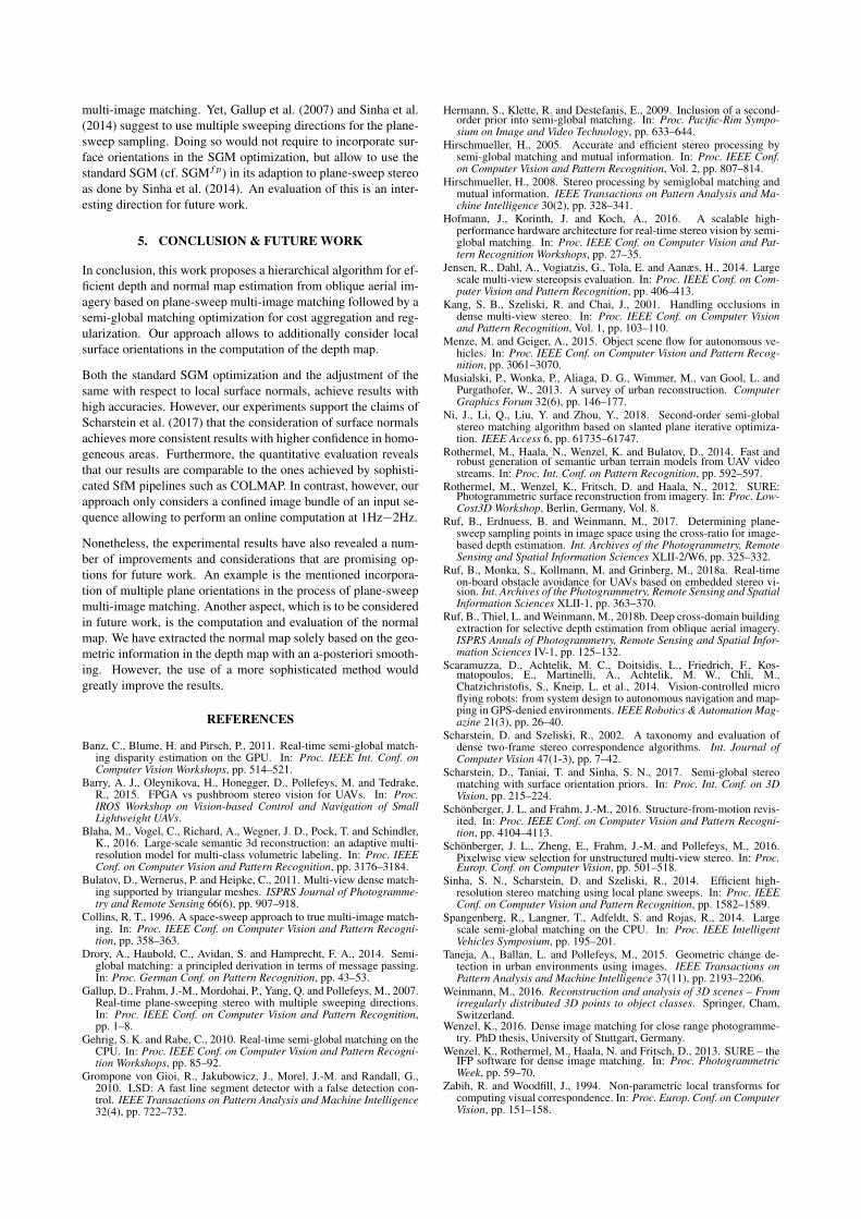
with Γ(·) being a function that returns the index of Πd within theset of sampling planes (cf. Figure 2(b)).

In our second extension, namely surface normal SGM (SGMsn),we adopt the approach presented by Scharstein et al. (2017) to usesurface normals to adjust the zero-cost transition to coincide withthe surface orientation. We use a normal mapN corresponding toIref that holds the surface normals of the scene that is to be recon-structed. We assume N to be given or use the normal map thathas been predicted in the previous iteration of our hierarchicalwork flow (cf. Figure 1). Assuming that a surface normal vectornp = N(p) corresponding to the surface orientation at pixel p isgiven, we compute the discrete index jump ∆isn through the setof sampling planes that is caused by the tangent plane to np at thescene point Xp, in which the ray through p intersects Πd. As alsostated by Scharstein et al. (2017), these discrete index jumps canbe computed once for each pixel p and each path direction r (cf.Figure 2(c)). Given ∆isn, we adjust the smoothness term used inSGMsn according to

Vsn(Πd,Πd′) = Vfp(Πd + ∆isn,Πd′). (7)

The third extension does not consider any additional information,such as surface normalsN , while computing the aggregating pathcosts Lr(p,Πd). Instead, it relies on the gradient ∇r in scenespace corresponding to the minimal path costs and is therefore de-noted as path gradient SGM (SGMpg). Here, we again considerXp as the scene point corresponding to the intersection betweenthe ray through p and Πd. Furthermore, we denote p′ = p + r

as predecessor of p along the path r and Xp′ as the scene pointparameterized by p′ and the plane Πd. The latter represents theplane at depth d = arg mind′∈D Lr(p

′,Πd′) associated with theprevious minimal path costs. From this, we dynamically computea gradient vector∇r = Xp− Xp′ in scene space while traversingalong the path r. Given ∇r, we again compute a discrete indexjump ∆ipg through the set of sampling planes and use

Vpg(Πd,Πd′) = Vfp(Πd + ∆ipg,Πd′) (8)

to dynamically adjust the zero-cost transition to possibly slantedsurfaces in scene space (cf. Figure 2(d)). This allows us to im-plicitly penalize deviations from the running gradient vector inscene space between two consecutive pixels along the path r.

Since our extensions SGMx only affect the path-wise aggregationof the matching costs, we extract the depth map D analogouslyto Equation (3) and Equation (4), substituting the disparity by thedepths corresponding to the set of sampling planes. Note that,since our sampling set consists of fronto-parallel planes, we candirectly extract the depth from their parameterization. If slantedplanes are used for sampling, a pixel-wise intersection of theviewing rays with the winning planes is to be performed in or-der to extract D.

Finally, for each of the extensions, a median filter with a kernelsize of 5× 5 is used to further reduce noise.

3.3 Adaptive smoothness penalty

Hirschmueller (2005, 2008) suggests to adaptively adjust thepenalty P2 to the image gradient along path r in order to pre-serve depth discontinuities at object boundaries. In this work, weevaluate two different strategies to adjust P2. The first strategyfully relies on the absolute intensity difference (|∆I|) betweenconsecutive pixels:

P∆I2 = P1

(1 + α exp

(−|∆I|

β

))(9)

with α = 8 and β = 10 according to Scharstein et al. (2017).

A second strategy that has been proposed by Ruf et al. (2018b)relies on the use of a line segment detector (Grompone von Gioiet al., 2010) to generate a binary line image of the reference imageIlineref and reduce P line

2 to P1 at a detected line segment:

P line2 =

{P1 , if Iline

ref (p) = 1

P2 , otherwise.(10)

Ruf et al. (2018b) argue that this allows to enforce strong dis-continuities at object boundaries while increasing the smoothnesswithin objects.

3.4 Confidence measure

We additionally compute a confidence map C, holding per-pixelconfidence measures of the depth estimates in the range of [0, 1].For this, we model two confidence measures that solely rely onthe results of the SGM path aggregation. With our first measureUp, we adopt the observation of Drory et al. (2014), that the sumof the individual minimal path costs at pixel p is a lower boundof the winning aggregated costs:

Up = mindS(p,Πd)−

∑r

mindLr(p,Πd). (11)

p p′ = p + r

r

Π𝑑

𝒮 p,Π𝑑

𝒮 p′, Π𝑑

𝒮 p′, Π𝑑 − 1

𝒮 p′, Π𝑑 + 1

𝒮 p′, Π𝑑 + 2

p p′ = p + r

r

Π𝑑

𝒮 p,Π𝑑

𝒮 p′, Π𝑑 + Δ𝑖𝑠𝑛

𝒮 p′, Π𝑑 + Δ𝑖𝑠𝑛 − 1

𝒮 p′, Π𝑑 + Δ𝑖𝑠𝑛 + 1

np Δ𝑖𝑠𝑛

p p′ = p + r

r

Π𝑑

𝒮 p,Π𝑑

∇r

𝒮 p′, Π𝑑 + Δ𝑖𝑝𝑔

𝒮 p′, Π𝑑 + Δ𝑖𝑝𝑔 − 1

𝒮 p′, Π𝑑 + Δ𝑖𝑝𝑔 + 1

Δ𝑖𝑝𝑔

- - - - - - Minimum Cost Path 𝐿r p,Π𝑑

(a) (b) (c) (d)

Figure 2. Illustration of the SGMx path aggregation along one path direction r. (a) Normal map of a building. The yellow line indicates the areafor which the SGMx path aggregation is shown. (b) Illustration of the SGMfp path aggregation. The blue and pink lines correspond to blue and pinksurface orientations on the building facade. When aggregating the path costs for pixel p at plane Πd, SGMfp will incorporate the previous costs at thesame plane position (green) without additional penalty. The previous path costs at Πd ± 1 (yellow) will be penalized with P1. The previous path costslocated at Πd + 2 (red), which is actually located on the corresponding surface, will be penalized with the highest penalty P2. (c) SGMsn uses thenormal vector np, encoding the surface orientation at pixel p, and computes a discrete index jump ∆isn, which adjusts the zero cost transition, causingthe previous path costs at Πd + 2 to not be penalized. (d) Similar to SGMsn, SGMpg adjusts the zero cost transition. However, the discrete index jump∆ipg is derived from the running gradient ∇r of the minimum cost path. As illustrated, however, this can overcompensate the shift of the zero costtransition.

The second confidence measure Uu models the uniqueness of thewinning aggregated costs, i.e. the difference between the lowestand second-lowest aggregated costs for each pixel in S:

Uu = mind

(S(p,Πd)\min

dS(p,Πd)

)−

mindS(p,Πd).

(12)

Given the above measures, we compute the final pixel-wise con-fidence value according to

C(p) = exp

(−Up

ϕ

)·min {exp (Uu − τ) , 1} . (13)

In this equation, the first term will resolve to 1, if Up = 0, i.e. thewinning costs equal the sum of the minimal path costs. If this isnot the case, the rate of the exponential decay of the confidenceis controlled by the parameter ϕ.

The parameter τ represents the uniqueness threshold of the win-ning solution. If the absolute difference between the lowestand second-lowest pixel-wise aggregated costs in S is above thethreshold τ , the second term of Equation (13) will resolve to 1.

In our evaluation, this confidence measure is used to plot the ac-curacy of the predicted depth maps with respect to their com-pleteness, where the latter is computed by thresholding the corre-sponding confidence map (cf. Figure 3(b)).

3.5 Normal map estimation

The third output of our algorithm is a normal map N that holdsthe surface orientation in the depth map D at pixel p. For thecomputation of the surface normal, we reproject the depth mapinto a point cloud and compute the cross product np = hp × vp.Here, hp denotes a vector between the scene points of two neigh-boring pixels to p in horizontal direction, while vp is the vectorbetween the scene points of two vertical neighboring pixels.

Since the computation of N does not contain any smoothness as-sumption, we apply an a-posteriori smoothing to the normal map,the so-called Gestalt-Smoothing. In particular, we perform anappearance-based weighted Gaussian smoothing in a local two-dimensional neighborhoodNp around p:

N(p) =np

|np|, (14)

with

np = np +∑

q∈Np

[nq ·

1√2πσ2

exp

(− (q− p)2

2σ2

)

· exp

(−|Iq − Ip|

β

)],

(15)

where β = 10 in accordance with Equation (9), and σ is fixed tothe radius of the local smoothing neighborhood.

4. EVALUATION

4.1 Experiments

We have evaluated our approach on two different datasets,namely the DTU Robot Multi-View Stereo (MVS) dataset(Jensen et al., 2014) and a private dataset, which is henceforthreferred to as the TMB dataset.

From the DTU dataset, we have selected 21 scans of the differ-ent building models, in which each model was captured from 49locations and with eight different lighting conditions. For ourevaluation, we have used the already undistorted images with aresolution of 1600×1200 pixels, captured under the most diffuselighting. As ground truth to our approach, we have extracteddepth maps from the structured light scans, which are includedin the dataset, given the camera poses of the reference image.

Our privately captured TMB dataset consists of three differentscenes captured with a DJI Phantom 3 Professional from multipledifferent aerial viewpoints. The images were captured while fly-ing around the objects of interest at three different altitudes (8 m,10 m and 15 m). Each image was resized to 1920×1080 pixelsbefore used for our evaluation. We compare the results achievedby the proposed approach to data from an offline SfM pipelinefor accurate and dense 3D image matching. For this, we haveused COLMAP (Schonberger and Frahm, 2016; Schonberger etal., 2016) to reconstruct the considered scenes of the dataset.As a required input to our algorithm, we have used the cameraposes computed by the sparse reconstruction. In the evaluation,we have compared the depth maps predicted by our algorithmagainst the geometric depth maps from the dense reconstructionof COLMAP.

As an accuracy measure between the estimates and the groundtruth, we have used an absolute and relative L1 measure, which is

DTU TMB

Configuration Name mL1-abs mL1-rel mL1-abs mL1-rel

SGMfp-CT-P∆I2 10.362±11.867 0.014±0.015 0.392±0.336 0.712±0.486

SGMfp-CT-P line2 10.392±12.065 0.014±0.015 0.406±0.358 0.713±0.485

SGMfp-NCC-P∆I2 9.859±11.781 0.014±0.015 0.406±0.347 0.704±0.480

SGMfp-NCC-P line2 12.588±13.493 0.017±0.017 0.492±0.435 0.704±0.461

SGMsn-CT-P∆I2 10.106±11.532 0.014±0.015 0.401±0.349 0.717±0.489

SGMsn-CT-P line2 10.292±12.068 0.014±0.016 0.412±0.367 0.718±0.489

SGMsn-NCC-P∆I2 9.770±11.850 0.013±0.015 0.411±0.351 0.705±0.479

SGMsn-NCC-P line2 12.402±13.405 0.017±0.017 0.491±0.434 0.704±0.460

SGMpg-CT-P∆I2 10.612±11.919 0.015±0.015 0.401±0.339 0.718±0.493

SGMpg-CT-P line2 10.529±12.014 0.015±0.015 0.413±0.359 0.712±0.492

SGMpg-NCC-P∆I2 10.010±11.739 0.014±0.015 0.417±0.344 0.710±0.481

SGMpg-NCC-P line2 12.598±13.358 0.017±0.017 0.495±0.432 0.706±0.461

COLMAP 3.309±4.156 0.005±0.006 - -

(a) Quantitative results of all twelve configurations which are evaluated on the DTUand TMB dataset. For each dataset, the mean absolute L1 error (mL1-abs) as well asthe mean relative L1 error (mL1-rel) are evaluated. The configuration name encodesthe different configuration settings. Here, the first part represents the extension used,the middle section holds the cost function which was applied in the multi-imagematching, and the third portion represents the strategy, which was adopted to adaptthe P2 penalty. The last row denotes the results achieved by the offline SfM pipelineCOLMAP (Schonberger and Frahm, 2016; Schonberger et al., 2016).

0.0 0.2 0.4 0.6 0.8 1.0Confidence Threshold

DTU

0.000

0.002

0.004

0.006

0.008

0.010

mL

1-re

l·D

ensi

ty

SGMfp-NCC-P∆I2

SGMsn-NCC-P∆I2

SGMpg-NCC-P∆I2

0.0 0.2 0.4 0.6 0.8 1.0Confidence Threshold

TMB

0.0

0.1

0.2

0.3

0.4

0.5

0.6

0.7

mL

1-re

l·D

ensi

ty

SGMfp-NCC-P∆I2

SGMsn-NCC-P∆I2

SGMpg-NCC-P∆I2

(b) ROC curves plotting normalized mean L1-rel over theconfidence threshold which is used to mask the depth map.The top graph depicts the results achieved by three SGMx

configurations on the DTU dataset. The bottom graph showsthe results achieved on the TMB dataset.

Figure 3. Quantitative evaluation of twelve different SGMx configurations.

computed pixel-wise and averaged over the number of estimatesin the depth map:

L1-abs(d, d) =1

m

∑i

|di − di|, (16)

L1-rel(d, d) =1

m

∑i

|di − di|di

, (17)

with d and d denoting the predicted and ground truth depth valuesrespectively, and with m being the number of pixels for whichboth d and d exists. Here, the depth values denote the fronto-parallel distances of the corresponding scene points from the im-age center of the reference camera. Both measures are only eval-uated for pixels which contain a predicted and ground truth depthvalue. While L1-abs denotes the average absolute difference be-tween the prediction and the ground truth, L1-rel computes thedepth error relative to the ground truth depth. This reduces theinfluence of a high absolute error where the ground truth depthis large and increases the influence of measurements close to thecamera. This is important, as the uncertainty of the depth mea-surements typically increases with the distance from the camera.

The parameterization of our algorithms was determined empir-ically based on the results, which were achieved on the DTUdataset. For our hierarchical processing scheme, we have usedL = 3 pyramid levels and have set ∆d = 6 for the computa-tion of the per-pixel sampling range, yielding the best trade-offbetween accuracy and runtime. The support region of the nor-malized cross correlation (NCC) and the Census Transform (CT)was set to 5×5 and 9×7, respectively, where the latter is the max-imum size for which the CT bit string still fits into a 64 bit integer.

In the computation of the normal map, we have used a smoothingkernel of size 21×21 for the Gestalt-Smoothing.

Due to the different range of values in the cost functions, theparameterization of the penalty functions and the confidencemeasures need to be chosen accordingly. For the NCC simi-larity measure, we have set P1 = 150 when using P∆I

2 andP1 = 60, P2 = 220 when using P line

2 . In case of the CT, wehave set P1 = 15 when using P∆I

2 and P1 = 10, P2 = 55 whenusing P line

2 . For the computation of the confidence measure (cf.Equation (13)), we have set ϕ = 80, τ = 10 when using theNCC, and ϕ = 650, τ = 80 when using the CT.

All experiments were performed on a desktop hardware with anIntel Core i7-5820K CPU 3.3GHz and a NVIDIA GeForce GTX1070 GPU. The computationally expensive part of our algorithm,such as depth and normal map estimation, is optimized withCUDA to run on the GPU, achieving a frame rate of 1Hz−2Hzfor full HD imagery, depending on the configuration and param-eterization used.

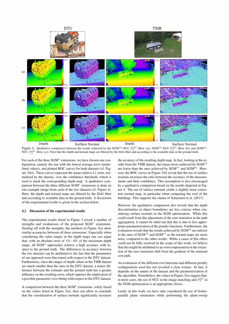
In the scope of this work, we have evaluated twelve differentconfigurations of our SGMx extensions. The results achievedby these configurations on the two datasets are listed in Fig-ure 3(a). The configuration names denote the corresponding se-tups. In comparison, the results achieved by the offline SfMpipeline COLMAP are listed in the last row of Figure 3(a). Thevalues in the depth maps are in the range of [554.1, 846.5] in caseof the DTU dataset, and [2.0, 10] in the depth maps correspond-ing to the TMB dataset (cf. Figure 4). Since the datasets do nothave any metric system, the errors are without any unit. How-ever, the given ranges of values in the depth maps allow to drawconclusions on these error values with respect to the estimates.

DTU TMB

(a)

(b)

(c)

Surface Normal Depth Surface Normal

554.1

846.5

554.1

846.5

Depth554.1

846.5

2.0

10.0

2.0

10.0

2.0

10.0

Figure 4. Qualitative comparison between the results achieved by the SGMfp-NCC-P∆I2 (Row (a)), SGMsn-NCC-P∆I

2 (Row (b)) and SGMpg-NCC-P∆I

2 (Row (c)). Note that the depth and normal maps are filtered by the DoG filter and according to the available data in the ground truth.

For each of the three SGMx extensions, we have chosen one con-figuration, namely the one with the lowest average error (under-lined values), and plotted ROC curves for both datasets (cf. Fig-ure 3(b)). These curves represent the mean relative L1 error, nor-malized by the density, over the confidence threshold, which isused to mask the corresponding depth map. A qualitative com-parison between the three different SGMx extensions is done onone example image from each of the two datasets (cf. Figure 4).Here, the depth and normal maps are filtered by the DoG filterand according to available data in the ground truth. A discussionof the experimental results is given in the section below.

4.2 Discussion of the experimental results

The experimental results listed in Figure 3 reveal a number ofstrengths and weaknesses of the proposed SGMx extensions.Starting off with the strengths, the numbers in Figure 3(a) showsimilar accuracies between all three extensions. Especially whenconsidering the value ranges in the depth maps one can arguethat, with an absolute error of 1%−4% of the maximum depthrange, all SGMx approaches achieve a high accuracy with re-spect to the ground truth. The differences in accuracy betweenthe two datasets can be attributed to the fact that the parametersof our approach were fine-tuned with respect to the DTU dataset.Furthermore, since the ranges of depth values in the TMB datasetare much smaller than the ones in the DTU dataset, a minor dif-ference between the estimate and the ground truth has a greaterinfluence on the resulting error, which opposes the implication ofa possible parametric over-fitting with respect to the DTU dataset.

A comparison between the three SGMx extensions, solely basedon the values listed in Figure 3(a), does not allow to concludethat the consideration of surface normals significantly increases

the accuracy of the resulting depth map. In fact, looking at the re-sults from the TMB dataset, the mean errors achieved by SGMfp

are lower than the ones achieved by SGMsn and SGMpg . How-ever, the ROC curves in Figure 3(b) reveal that the use of surfacenormals increases the ratio between the accuracy of the measure-ments and their confidence. This assumption is also encouragedby a qualitative comparison based on the results depicted in Fig-ure 4. The use of surface normals yields a slightly more consis-tent normal map, in particular when comparing the roof of thebuildings. This supports the claims of Scharstein et al. (2017).

However, the qualitative comparison also reveals that the depthdiscontinuities at object boundaries are less concise when con-sidering surface normals in the SGM optimization. While thiscould result from the adjustment of the zero transition in the pathaggregation, it cannot be ruled out that this is due to less appro-priate parameterization of the penalty functions. Furthermore, theevaluation reveals that the results achieved by SGMpg are inferiorto the ones of SGMfp and SGMsn as the normal maps are morenoisy compared to the other results. While a cause of this effectcould not be fully resolved in the scope of this work, we believethat this might be attributed to an overcompensation in the extrac-tion of the zero transition shift from the gradient of the minimalcost path.

An evaluation of the different cost functions and different penaltyconfigurations used has not revealed a clear winner. In fact, itdepends on the nature of the dataset and the parameterization ofthe algorithm. Nonetheless, the values in Figure 3(a) suggest that,in most cases, the use of NCC in the image matching and P∆I

2 inthe SGM optimization is an appropriate choice.

Lastly, in this work, we have only considered the use of fronto-parallel plane orientation while performing the plane-sweep

multi-image matching. Yet, Gallup et al. (2007) and Sinha et al.(2014) suggest to use multiple sweeping directions for the plane-sweep sampling. Doing so would not require to incorporate sur-face orientations in the SGM optimization, but allow to use thestandard SGM (cf. SGMfp) in its adaption to plane-sweep stereoas done by Sinha et al. (2014). An evaluation of this is an inter-esting direction for future work.

5. CONCLUSION & FUTURE WORK

In conclusion, this work proposes a hierarchical algorithm for ef-ficient depth and normal map estimation from oblique aerial im-agery based on plane-sweep multi-image matching followed by asemi-global matching optimization for cost aggregation and reg-ularization. Our approach allows to additionally consider localsurface orientations in the computation of the depth map.

Both the standard SGM optimization and the adjustment of thesame with respect to local surface normals, achieve results withhigh accuracies. However, our experiments support the claims ofScharstein et al. (2017) that the consideration of surface normalsachieves more consistent results with higher confidence in homo-geneous areas. Furthermore, the quantitative evaluation revealsthat our results are comparable to the ones achieved by sophisti-cated SfM pipelines such as COLMAP. In contrast, however, ourapproach only considers a confined image bundle of an input se-quence allowing to perform an online computation at 1Hz−2Hz.

Nonetheless, the experimental results have also revealed a num-ber of improvements and considerations that are promising op-tions for future work. An example is the mentioned incorpora-tion of multiple plane orientations in the process of plane-sweepmulti-image matching. Another aspect, which is to be consideredin future work, is the computation and evaluation of the normalmap. We have extracted the normal map solely based on the geo-metric information in the depth map with an a-posteriori smooth-ing. However, the use of a more sophisticated method wouldgreatly improve the results.

REFERENCES

Banz, C., Blume, H. and Pirsch, P., 2011. Real-time semi-global match-ing disparity estimation on the GPU. In: Proc. IEEE Int. Conf. onComputer Vision Workshops, pp. 514–521.

Barry, A. J., Oleynikova, H., Honegger, D., Pollefeys, M. and Tedrake,R., 2015. FPGA vs pushbroom stereo vision for UAVs. In: Proc.IROS Workshop on Vision-based Control and Navigation of SmallLightweight UAVs.

Blaha, M., Vogel, C., Richard, A., Wegner, J. D., Pock, T. and Schindler,K., 2016. Large-scale semantic 3d reconstruction: an adaptive multi-resolution model for multi-class volumetric labeling. In: Proc. IEEEConf. on Computer Vision and Pattern Recognition, pp. 3176–3184.

Bulatov, D., Wernerus, P. and Heipke, C., 2011. Multi-view dense match-ing supported by triangular meshes. ISPRS Journal of Photogramme-try and Remote Sensing 66(6), pp. 907–918.

Collins, R. T., 1996. A space-sweep approach to true multi-image match-ing. In: Proc. IEEE Conf. on Computer Vision and Pattern Recogni-tion, pp. 358–363.

Drory, A., Haubold, C., Avidan, S. and Hamprecht, F. A., 2014. Semi-global matching: a principled derivation in terms of message passing.In: Proc. German Conf. on Pattern Recognition, pp. 43–53.

Gallup, D., Frahm, J.-M., Mordohai, P., Yang, Q. and Pollefeys, M., 2007.Real-time plane-sweeping stereo with multiple sweeping directions.In: Proc. IEEE Conf. on Computer Vision and Pattern Recognition,pp. 1–8.

Gehrig, S. K. and Rabe, C., 2010. Real-time semi-global matching on theCPU. In: Proc. IEEE Conf. on Computer Vision and Pattern Recogni-tion Workshops, pp. 85–92.

Grompone von Gioi, R., Jakubowicz, J., Morel, J.-M. and Randall, G.,2010. LSD: A fast line segment detector with a false detection con-trol. IEEE Transactions on Pattern Analysis and Machine Intelligence32(4), pp. 722–732.

Hermann, S., Klette, R. and Destefanis, E., 2009. Inclusion of a second-order prior into semi-global matching. In: Proc. Pacific-Rim Sympo-sium on Image and Video Technology, pp. 633–644.

Hirschmueller, H., 2005. Accurate and efficient stereo processing bysemi-global matching and mutual information. In: Proc. IEEE Conf.on Computer Vision and Pattern Recognition, Vol. 2, pp. 807–814.

Hirschmueller, H., 2008. Stereo processing by semiglobal matching andmutual information. IEEE Transactions on Pattern Analysis and Ma-chine Intelligence 30(2), pp. 328–341.

Hofmann, J., Korinth, J. and Koch, A., 2016. A scalable high-performance hardware architecture for real-time stereo vision by semi-global matching. In: Proc. IEEE Conf. on Computer Vision and Pat-tern Recognition Workshops, pp. 27–35.

Jensen, R., Dahl, A., Vogiatzis, G., Tola, E. and Aanæs, H., 2014. Largescale multi-view stereopsis evaluation. In: Proc. IEEE Conf. on Com-puter Vision and Pattern Recognition, pp. 406–413.

Kang, S. B., Szeliski, R. and Chai, J., 2001. Handling occlusions indense multi-view stereo. In: Proc. IEEE Conf. on Computer Visionand Pattern Recognition, Vol. 1, pp. 103–110.

Menze, M. and Geiger, A., 2015. Object scene flow for autonomous ve-hicles. In: Proc. IEEE Conf. on Computer Vision and Pattern Recog-nition, pp. 3061–3070.

Musialski, P., Wonka, P., Aliaga, D. G., Wimmer, M., van Gool, L. andPurgathofer, W., 2013. A survey of urban reconstruction. ComputerGraphics Forum 32(6), pp. 146–177.

Ni, J., Li, Q., Liu, Y. and Zhou, Y., 2018. Second-order semi-globalstereo matching algorithm based on slanted plane iterative optimiza-tion. IEEE Access 6, pp. 61735–61747.

Rothermel, M., Haala, N., Wenzel, K. and Bulatov, D., 2014. Fast androbust generation of semantic urban terrain models from UAV videostreams. In: Proc. Int. Conf. on Pattern Recognition, pp. 592–597.

Rothermel, M., Wenzel, K., Fritsch, D. and Haala, N., 2012. SURE:Photogrammetric surface reconstruction from imagery. In: Proc. Low-Cost3D Workshop, Berlin, Germany, Vol. 8.

Ruf, B., Erdnuess, B. and Weinmann, M., 2017. Determining plane-sweep sampling points in image space using the cross-ratio for image-based depth estimation. Int. Archives of the Photogrammetry, RemoteSensing and Spatial Information Sciences XLII-2/W6, pp. 325–332.

Ruf, B., Monka, S., Kollmann, M. and Grinberg, M., 2018a. Real-timeon-board obstacle avoidance for UAVs based on embedded stereo vi-sion. Int. Archives of the Photogrammetry, Remote Sensing and SpatialInformation Sciences XLII-1, pp. 363–370.

Ruf, B., Thiel, L. and Weinmann, M., 2018b. Deep cross-domain buildingextraction for selective depth estimation from oblique aerial imagery.ISPRS Annals of Photogrammetry, Remote Sensing and Spatial Infor-mation Sciences IV-1, pp. 125–132.

Scaramuzza, D., Achtelik, M. C., Doitsidis, L., Friedrich, F., Kos-matopoulos, E., Martinelli, A., Achtelik, M. W., Chli, M.,Chatzichristofis, S., Kneip, L. et al., 2014. Vision-controlled microflying robots: from system design to autonomous navigation and map-ping in GPS-denied environments. IEEE Robotics & Automation Mag-azine 21(3), pp. 26–40.

Scharstein, D. and Szeliski, R., 2002. A taxonomy and evaluation ofdense two-frame stereo correspondence algorithms. Int. Journal ofComputer Vision 47(1-3), pp. 7–42.

Scharstein, D., Taniai, T. and Sinha, S. N., 2017. Semi-global stereomatching with surface orientation priors. In: Proc. Int. Conf. on 3DVision, pp. 215–224.

Schonberger, J. L. and Frahm, J.-M., 2016. Structure-from-motion revis-ited. In: Proc. IEEE Conf. on Computer Vision and Pattern Recogni-tion, pp. 4104–4113.

Schonberger, J. L., Zheng, E., Frahm, J.-M. and Pollefeys, M., 2016.Pixelwise view selection for unstructured multi-view stereo. In: Proc.Europ. Conf. on Computer Vision, pp. 501–518.

Sinha, S. N., Scharstein, D. and Szeliski, R., 2014. Efficient high-resolution stereo matching using local plane sweeps. In: Proc. IEEEConf. on Computer Vision and Pattern Recognition, pp. 1582–1589.

Spangenberg, R., Langner, T., Adfeldt, S. and Rojas, R., 2014. Largescale semi-global matching on the CPU. In: Proc. IEEE IntelligentVehicles Symposium, pp. 195–201.

Taneja, A., Ballan, L. and Pollefeys, M., 2015. Geometric change de-tection in urban environments using images. IEEE Transactions onPattern Analysis and Machine Intelligence 37(11), pp. 2193–2206.

Weinmann, M., 2016. Reconstruction and analysis of 3D scenes – Fromirregularly distributed 3D points to object classes. Springer, Cham,Switzerland.

Wenzel, K., 2016. Dense image matching for close range photogramme-try. PhD thesis, University of Stuttgart, Germany.

Wenzel, K., Rothermel, M., Haala, N. and Fritsch, D., 2013. SURE – theIFP software for dense image matching. In: Proc. PhotogrammetricWeek, pp. 59–70.

Zabih, R. and Woodfill, J., 1994. Non-parametric local transforms forcomputing visual correspondence. In: Proc. Europ. Conf. on ComputerVision, pp. 151–158.