August 2011

EFFICIENT REDISTRIBUTION OF LIFETIME INCOME

THROUGHWELFARE ACCOUNTS

A. Lans Bovenberg, CentER, Tilburg University,

Netspar, CEPR and CESifo

Martin Ino Hansen, Danish Ministry of Social Affairs

Peter Birch Sørensen, University of Copenhagen, CESifo and Netspar

Abstract: Compared to a conventional tax-transfer system, individual welfare accounts can

redistribute lifetime incomes at a lower efficiency cost. These welfare accounts employ manda-

tory contributions rather than taxes to finance social transfers to people of working age. We

describe a design for the welfare accounts that guarantees a Pareto improvement if behavioural

responses to the accounts improve the public budget. We also develop a formula for quantifying

the impact of welfare accounts on the government budget and economic efficiency. Applying the

formula to Danish data, we find that the proposed welfare accounts would generate a Pareto

improvement, thus improving the trade-off between equity and efficiency. We discuss how the

gains from welfare accounts can be distributed in an equitable manner.

Keywords: Social insurance, welfare accounts, lifetime income distribution

JEL Code: H53, H55

Corresponding author:

Peter Birch Sørensen

Department of Economics, University of Copenhagen

Øster Farimagsgade 5, 1353 Copenhagen K, Denmark.

E-mail: pbs@econ.ku.dk

EFFICIENT REDISTRIBUTION

OF LIFETIME INCOME

THROUGH WELFARE ACCOUNTS:

A. Lans Bovenberg, Martin Ino Hansen and Peter Birch Sørensen1

1. The problem: Can lifetime incomes be redistributed at a lower

efficiency cost?

The Western European welfare states collect substantial tax revenues to finance social

transfers intended to redistribute income towards various needy groups. Yet, despite the

huge sums involved, these tax-transfer programmes achieve only a limited redistribution

of income from the lifetime rich to the lifetime poor. For example, in Denmark, which is

considered to be one of the world’s most ambitious welfare states, about three fourths of

the taxes collected to finance the various social transfers is estimated to be paid back to

the individual taxpayer himself via various benefits received at different points in the life

cycle. Hence, only about one-fourth of the taxes collected to finance the Danish social

insurance programs serves to redistribute resources from those with high to those with

low lifetime incomes, as we have shown in Bovenberg, Hansen and Sørensen (2008). In

that paper we also review several studies indicating a limited degree of lifetime income

redistribution in other OECD countries. For instance, for the UK, Falkingham and

Harding (1996) found that only between 29 and 38 percent of the taxes levied to finance

social transfers represent so-called inter-personal redistribution, i.e., redistribution of

lifetime income.

Though a large part of an individual’s tax payments and social security contributions

is recycled to himself via social transfers received over the life course, these taxes and

benefits nevertheless distort behaviour. The reason is that a direct actuarial link be-

tween taxes paid and benefits received is typically lacking. This paper proposes a tax

and benefit reform eliminating a major part of the tax distortions and moral hazard

1Thanks are due to Giuseppe Bertola, Antoine Bozio, Christian Gollier, Jukka Lassila, Hans-Werner

Sinn and an anonymous referee for comments on earlier drafts of this paper. They should not be held

responsible for any remaining shortcomings.

2

effects caused by taxes and benefits that redistribute income mainly over the taxpayer’s

own life cycle rather than between citizens with different lifetime incomes. The reform

involves the introduction of welfare accounts. These are mandatory individual savings

accounts financing social transfers that are returned to the taxpayer at some other stage

in the life cycle. The welfare accounts create an actuarial link between contributions paid

and benefits received, thereby preventing distortions arising from purely intra-personal

redistribution (i.e., redistribution over the life cycle). The fraction of social benefits rep-

resenting inter-personal redistribution of lifetime income remains tax-financed and thus

continues to generate distortions, reflecting the inescapable efficiency cost of redistribu-

tion from the lifetime rich to the lifetime poor.

Our reform proposal should allow policy makers to achieve the desired degree of

lifetime income redistribution in a more efficient manner. It may be seen as a complement

to the recent Mirrlees Review (2011), which proposes several changes to the personal tax

system to facilitate the smoothing of taxable income so that the progressivity of the

income tax becomes better targeted at individuals with high lifetime incomes rather

than at those with temporarily high annual incomes. Also the Mirrlees Review (2011, ch.

5) argues for an integration of social transfers with the personal tax system to achieve a

more coherent system of social insurance and redistribution. Our account system is an

example of how such an integration could be achieved.

Compared to the previous literature on mandatory individual savings accounts for

social insurance, this paper makes two main contributions. First, we describe a new

design for welfare accounts guaranteeing a Pareto improvement provided the account

system generates behavioral responses that result in an improvement in the public budget.

Second, we derive a formula for estimating whether a system of welfare accounts will in

fact yield a positive net impact on the public budget, once the behavioural responses

are accounted for. We apply our formula to data for Denmark and show that even with

conservative assumptions regarding the relevant labour supply elasticities our blueprint

for welfare accounts is highly likely to generate a Pareto improvement.

A large literature exists on the costs and benefits of using individual saving accounts

to finance social security for the (retired) elderly. Much of this literature has debated

whether pensions should be fully pre-funded or financed on a pay-as-you go basis, and

3

whether they should be based on defined contributions or on defined benefits. Feldstein

(2005) and Barr and Diamond (2008) represent differing viewpoints on these matters.

The present paper does not discuss the issue of old-age social security. Instead, we focus

on social transfers to people of working age. Furthermore, although our welfare accounts

could be designed as a funded system, we assume here that they are implemented as

purely notional accounts, i.e., as book-keeping devices without accumulation of funds for

investment. As we shall explain, these accounts can be introduced without involving any

redistribution across generations.

The literature on the potential role of individual accounts in providing social in-

surance for the working population is relatively sparse. Fölster (1997, 1999), Orszag

and Snower (1997, 2002), Feldstein and Altman (1998), Brown et al. (2006), Fölster

et al. (2002), Stiglitz and Yun (2002), and Bovenberg, Hansen and Sørensen (2008)

analyse the merits of various types of individual saving accounts. Some of these studies

investigate how individual accounts for the financing of unemployment benefits could

improve labour-market incentives, compared to a tax-financed system of unemployment

insurance. Fölster (1999) estimates how individual accounts financing a broader set of

social-insurance programs would affect the distribution of lifetime incomes in Sweden, as-

suming that the contributions to the accounts are set so as to leave the government budget

balance unaffected (before behavioural responses are allowed for). All of these studies

help to illuminate how the use of mandatory savings accounts for social insurance might

improve the equity-efficiency trade-off. However, unlike the present paper, these studies

do not analyse the conditions for a system of welfare accounts to be Pareto-improving.

The articles by Sørensen (2003) and Bovenberg and Sørensen (2004) do contain such an

analysis. This study extends the analysis in those papers to a more realistic setting and

presents a detailed empirical case study of how a system of welfare accounts might work

in practice.

Our paper is related to the literature on optimal unemployment insurance, to which

Hopenhayn and Nicolini (1997) made an important contribution. They found that when

the government cannot observe individual job search efforts, the optimal tax-benefit

scheme to insure against unemployment requires that workers who find a job should

pay a wage tax that increases with the length of their previous unemployment spell.

4

Although they are designed very differently than the tax-benefit scheme advocated by

Hopenhayn and Nicolini, our welfare accounts also have the property that net taxes paid

over the lifetime depend on the taxpayer’s history of earnings and benefit receipts. How-

ever, Shimer and Werning (2008) show that if workers are allowed to save and freely

borrow in a risk-free asset, a constant tax rate during employment and a constant ben-

efit rate during unemployment is the optimal policy. The savings accounts included in

Shimer’s and Werning’s optimal insurance program are reminiscent of the unemployment

insurance savings accounts proposed by Feldstein and Altman (2008) and the unemploy-

ment accounts considered in this paper. Still, our account system differs from the scheme

proposed by Shimer and Werning by placing restrictions on the amounts that account

holders can borrow from their accounts. As we shall see, such constraints are a necessary

consequence of the lifetime income insurance built into our account system.

Laroque (2010) recently proposed a system of notional welfare accounts (’social ac-

counts’ in his terminology) to keep track of each taxpayer’s net receipts from the public

sector. The balance on Laroque’s social accounts would provide information that would

enable the government to condition the size of an individual’s tax bill and transfer re-

ceipts on his/her earnings history and his/her accumulated receipts from the public sector.

However, Laroque refrains from spelling out exactly how the tax and benefit rules should

depend on the balance on the social account. Our specific proposal for a system of (no-

tional) welfare accounts is in the spirit of Laroque and has the same objective, i.e., to

improve the terms of the government’s trade-off between equity and efficiency.

The rest of the paper proceeds as follows. Section 2 describes the key features of

our proposed system of welfare accounts and explains its similarities with and differences

from some well-known alternative blueprints for social insurance. Section 3 presents a

formula that can be used to evaluate empirically whether the proposed welfare accounts

could generate a Pareto improvement. Section 4 applies this formula to a specific proposal

for a system of welfare accounts in Denmark. We estimate how this reform would affect

the distribution of lifetime incomes, the labour market, the public budget and economic

efficiency. Section 5 discusses how the efficiency gains from the welfare accounts could be

distributed in an equitable manner, and the concluding section 6 points to some social

trends that will tend to increase the gains from welfare accounts over time.

5

2. A design for welfare accounts

This section explains the principles underlying our proposed system of welfare accounts.

To motivate our proposal, we start by documenting the extent to which different social

transfer programmes succeed in redistributing lifetime incomes, using the Danish welfare

state as a case study. This analysis will help to identify the transfer programmes that

are most suitable for inclusion in the welfare account system.2

2.1. The redistributive impact of social transfer programmes

The degree of redistribution achieved through a transfer programme may be measured by

the redistribution index invented by Shorrocks (1982). The method used to calculate the

redistribution index is illustrated in Figure 1. Along the horizontal axis of the diagram

citizens are ordered in different percentile groups according to their disposable income.

As we move from left to right along the horizontal axis, disposable income increases. The

vertical axis measures the fraction of total transfers received by the various income groups

from some transfer programme. The so-called concentration curve drawn in the diagram

indicates the fraction of total benefits received by the poorestX percent of the population.

For example, point B on the concentration curve shows that the poorest 20 percent receive

40 percent of the benefits paid out under the hypothetical transfer programme considered.

If all individuals were to receive exactly the same amount of benefit under some transfer

programme, the concentration curve for that program would coincide with the 45-degree

line, since the poorest X percent would then always receive exactly X percent of total

benefits. If the concentration curve for a transfer programme lies above the diagonal, the

benefits from that programme tend to be concentrated among the lower income groups.

Such a programme will help to reduce the inequality in the distribution of disposable

incomes, compared to a programme that simply pays out the same lump-sum benefit to

everyone. Hence, we may use the area between the concentration curve and the 45-degree

line as a measure of the redistributive power of a transfer programme.

(Figure 1 about here)

2Part of this section borrows from Bovenberg and Sørensen (2007).

6

The redistribution indices shown in Table 1 have been calculated in this way.3 For

each of the Danish transfer programmes considered, the concentration curve and the

corresponding redistribution index were estimated using the distribution of annual dis-

posable incomes as well as the distribution of lifetime disposable incomes. The estimates

of lifetime incomes were taken from the report from the Danish Economic Council (2005,

ch. VI). They are based on a comprehensive micro panel data set covering the period

1994-2002 and comprising a sample of 10 percent of the Danish population above the

age of 18.4 Obviously, the higher the value of the redistribution index, the greater is

the redistribution achieved by the relevant transfer programme (in the Danish context

considered here, all transfers are financed out of general government revenues; to evaluate

the relative degrees of redistribution achieved by the various programmes, we thus do not

have to consider how they are financed).

(Table 1 about here)

In an annual perspective, we see that social assistance benefits and education benefits

are the most redistributive transfers. Also housing benefits and supplementary retirement

benefits (which are means-tested) exert a substantial redistributive impact on an annual

basis. In a lifetime perspective, most transfer programs yield a smaller effect on income

distribution. The exception here is the disability benefit, which is more redistributive in

a lifetime context because (in Denmark) relatively generous benefits are involved; so in

terms of annual income, the disabled are not among the poorest income groups. How-

ever, since disability typically involves a permanent loss of earnings capacity, the disabled

tend to end up with relatively low lifetime incomes. In a lifetime perspective, therefore,

disability benefits are more redistributive. A considerable part of housing benefits is

granted to recipients of disability benefits. This helps to explain why housing benefits

3To be quite precise, these redistribution indices are calculated as the area between the concentration

curve and the diagonal divided by the area below the diagonal (which is 12), so the value of the indices

is actually twice the area between the concentration curve and the diagonal.4The estimates were produced for the Danish Economic Council by Martin Ino Hansen working under

the supervision of Anne Kristine Høj and Peter Birch Sørensen. A detailed description of the method

used and an evaluation of the quality of the estimates is provided in a technical appendix available at

www.econ.ku.dk/pbs/.

7

are slightly more redistributive in a lifetime context than in an annual context. Unem-

ployment insurance benefits are also a bit more redistributive in a lifetime perspective,

because the incidence of long-term unemployment tends to be concentrated on unskilled

groups whose lifetime incomes are relatively low.

In general, the ranking of the various transfers according to their redistributive impact

changes significantly if the focus shifts from an annual to a lifetime measure of income.

Social assistance remains the most redistributive program, but its redistributive effect is

significantly smaller in a life-cycle context. Transfers such as parental leave benefits and

the basic retirement benefit (which is a flat benefit granted to all Danish residents above

the age of 65) have a significant impact on the distribution of annual incomes, but exert

(almost) the same effect on the distribution of lifetime incomes as an identical lump-sum

transfer to all individuals. The reason is that these benefits are granted in a phase of

the life cycle when people earn low annual incomes, thereby helping to reduce inequality

in annual incomes. However, the individuals who collect these benefits enjoy higher

incomes in other seasons of their life course, so these benefits do not contribute much

towards narrowing differences in lifetime incomes. The same type of argument holds even

more strikingly for grants to students in higher education. While such grants are highly

redistributive in an annual context, they yield only small effects on the distribution of

lifetime incomes.

The fact that many important transfer programmes result in very little redistribution

from the lifetime rich to the lifetime poor suggests that the financing and design of these

programs should be reconsidered. Moreover, the fact that many programs generate very

different redistributive impacts in an annual and in a lifetime perspective indicates the

importance of adopting a life-cycle perspective on the tax-transfer system. The blueprint

for reform presented below is guided by these insights.

2.2. A system of welfare accounts

The reform of the tax-transfer system to be analyzed in the rest of this paper has the

following key features:

1) For each citizen in the age group from, say, 18 years until the official retirement

age, a notional individual welfare account (WA) is established.

8

2) Each period, a mandatory social security contribution is credited to the WA. The

contribution is proportional to the account holder’s labour income (or active business

income of the self-employed).

3) The basic tax rate on labour income is lowered so that the sum of the labour

income tax bill and the new social security contribution is the same as the labour income

tax bill payable before the reform.

4) The account holder’s receipts of the social transfers included in the account system

(e.g. unemployment benefits, early retirement benefits etc.) are debited to the WA.

5) The social transfers included in the WA system can only be paid out subject to the

current eligibility rules (i.e., account holders cannot ’borrow’ freely from their accounts)

6) For married couples, contributions to the accounts are credited in equal amounts

to the WA of each spouse, and any benefit paid to one of the spouses is debited by half

the amount on the WA of each spouse. For unmarried parents any child-related benefits

are likewise debited by half the amount on the WA of each parent.

7) Each period an interest rate equal to the average after-tax interest rate on gov-

ernment bonds is added to positive WA account balances and subtracted from negative

account balances.

8) When an account holder reaches the official retirement age, his/her account is

settled. Any surplus on the WA at the date of retirement is either converted into an

annuity that is added to the ordinary public pension, or paid out as a lump sum. If

the account balance is negative at the time of retirement, it is set equal to zero and the

account holder still receives the full public pension stipulated by current rules.5

Several important properties of this account system are worth noting.

First, the WA system offers the same amount of liquidity insurance as the present

tax-transfer system. If account holders are exposed to a temporary income loss or a

temporary increase in their spending needs, they are eligible for receipt of social benefits

under exactly the same rules and criteria as at present.6

5Policy makers could decide that for persons choosing to work beyond the official retirement age, the

WA account balance will not be settled until the actual time of retirement.6The current benefit rules may well be in need of simplification, as argued by the Mirrlees Review

(2011) for the case of the UK. But in that case the rules should be simplified regardless of whether

welfare accounts are introduced.

9

Second, the WA system provides the same amount of lifetime income insurance as

the current fiscal system. Throughout his/her labour market career, each account holder

is eligible for the same social transfers as under the present system, and when retired,

his/her public pension cannot fall below the level guaranteed by current rules.

Third, no individual is forced to contribute a larger amount to the public sector, since

the contribution to the WA is matched by a corresponding cut in the labour income tax

bill.

Fourth, because the contribution to theWA is mandatory, the account system protects

myopic individuals who lack the foresight or the self-control needed to motivate them to

’save for a rainy day’.

Fifth, the account system ’bails out’ unlucky individuals and/or people with low life-

time incomes who end up with a negative WA balance, since these people will continue

to receive the normal public pension when they retire. Because of this ’bail-out’ clause,

account holders cannot be allowed to borrow freely (i.e. draw infinite amounts at their

own discretion) from their accounts. As mentioned, individuals can borrow from their ac-

counts only when they meet the current eligibility criteria for the social transfers included

in the WA system.

Sixth, for individuals who end up with an account surplus, the WAs establish an

actuarial link between contributions made and benefits received from the accounts. Each

pound contributed to the WA is returned to the account holder (with interest) either in

the form of benefits received during working age or in the form of an addition to the

public retirement benefit. In principle, the WAs thereby eliminate the current distortions

arising from the part of an individual’s tax bill that serves to finance transfers to himself

over his working career.

Seventh, for people ending up with an account surplus, any benefit drawn from the

WA implies an equivalent reduction in the present value of the payment from the account

at (or during) retirement. In this way, account holders effectively self-insure against the

income shortfalls or extra spending needs addressed by the various transfers included

in the WA system. This self-insurance limits the moral hazard associated with these

transfer programs by providing a strong incentive for account holders to avoid collecting

benefits unless they really need them.

10

Eighth, the provision under point 6) above should ensure a reasonably equal distrib-

ution of WA balances between men and women.

Ninth, since the notional WAs are merely a system of bookkeeping and not a funded

(investment-based) system of social insurance, the WA system does not require taxpay-

ers to set aside additional funds before they can draw benefits from the system. The

transition to the WA system can therefore proceed smoothly without the need for any

generations to finance benefits paid to other generations. For example, if all adults of

working age become subject to the new WA system from day one of the reform, people

close to retirement age at the time of reform would be able to accumulate only small WA

balances, but with the passing of time the WA balances paid out at retirement would

gradually increase as the younger cohorts would have had more time to accumulate their

balances.7

Tenth, in the WA system considered here, public retirement benefits are left un-

changed.8 Individuals with a WA surplus will simply receive a supplement to their

ordinary pension. If some workers who expect to end up with a WA surplus feel that

their total retirement income will exceed their needs, they can choose to reduce their net

savings via other channels.

Note that because of the features 3) and 8) above, the WA system described here can-

not make anyone worse off, but will make people with a WA surplus better off. Hence,

the system will generate a Pareto improvement unless it causes a deterioration of the

public budget that needs to be financed through higher taxes or spending cuts. If house-

holds do not change their behaviour in response to the WA system, the public budget

must necessarily deteriorate since people with a WA surplus receive a supplement to their

public pension while people with a WA deficit continue to pay the same total of tax and

social security contributions and collect the same benefits as today. The crucial question

7An alternative transition scheme would be to apply the WAs only to new young cohorts entering the

labour market after the time of reform. Again, this would mean that no generations would be forced to

finance benefits paid to other generations.8Factors such as demographic trends, globalisation, and growing public debt burdens may call for

reforms of the pension system, but here we leave this issue aside. Bovenberg and Sørensen (2004)

explain how retirement benefits could be included in a system of welfare accounts in a way that improves

the equity-efficiency trade-off without sacrificing the lifetime income insurance offered to low-income

earners.

11

is whether the behavioural responses to the WA system in the form of additional labour

supply and reduced take-up of benefits will be large enough to outweigh the ’mechani-

cal’ revenue loss that would occur with unchanged behaviour. Our analysis in section 4

suggests that this is indeed highly likely in the context of Denmark.

Before we proceed to this analysis, it may be useful to compare our WA system to

some alternative blueprints for social insurance. Table 2 compares a system of mandatory

individual accounts with a lifetime income guarantee (our ‘bail-out’ clause) to three other

ways of providing insurance against unexpected income losses: voluntary precautionary

saving, a ‘Bismarckian’ system of social insurance, and a ‘Beveridgean’ social insurance

system. In this terminology, a Bismarckian insurance system provides a clear actuarial

link at the individual level between insurance contributions paid and the value of the

insurance provided, whereas the Beveridgean social insurance system is redistributive,

involving flat social benefits financed by general tax revenues. Under both the Bismarck-

ian and Beveridgean systems, people are insured against the insured event and thus do

not pay themselves for the benefits they receive.

Under a system based on voluntary private saving, people are left to self-insure against

social events. Obviously, this limits the moral hazard problem discussed earlier, and it

also implies a strict actuarial link between benefits and contributions, since people finance

their ‘benefits’ out of their own saving. For these reasons a system based on voluntary

saving avoids the disincentives to work and preventive actions that are associated with a

redistributive public social insurance system. However, a major problem with voluntary

saving is that it does not provide liquidity insurance for those who have not managed

to save enough on their own account and cannot borrow against their expected future

income. Nor does reliance on voluntary saving address the problem that some individuals

may lack the necessary foresight to save enough, or the problem that some people may

strategically undersave in the expectation that the government will bail them out. Finally,

a system based on voluntary private saving obviously does not provide any redistribution

of lifetime income from rich to poor.

Compared to voluntary saving, mandatory individual accounts redistribute, offer liq-

uidity insurance and protect individuals lacking foresight or self control (the latter feature

is referred to as ‘paternalism’ in the third row of Table 2). Just as voluntary saving, in-

12

dividual accounts combat moral hazard and limit the disincentives to work for those who

can look forward to a surplus on their WAs.

The welfare accounts share with Bismarckian insurance the benefits of liquidity in-

surance and protection of myopic individuals. They differ from Bismarckian insurance in

two important respects. First, the accounts redistribute between the lifetime poor and

the lifetime rich by bailing out persons who end up with a negative balance at retirement.

The price of this redistribution is that the accounts do not provide an actuarial link for

the lifetime poor and therefore harm incentives for this group. The second difference from

Bismarckian insurance is that the accounts fight moral hazard because insurance benefits

are taken out of the individual accounts. The other side of this coin is that, compared

to Bismarckian insurance where people receive the full insurance benefit without having

to face a cut in their pension, the accounts provide less insurance for people who end up

with a positive account balance.

(Table 2 about here)

Thus, there are pros and cons with regard to all the different insurance mechanisms,

and an optimal overall system of social insurance is likely to involve some mix of the dif-

ferent mechanisms. The optimal mix will depend on country-specific circumstances and

on the specific type of risk against which protection is needed. The analysis below indi-

cates that mandatory individual savings accounts are a good way of providing insurance

in cases where the moral hazard problem associated with Beveridgean or Bismarckian

insurance is likely to be important, and where the income risks insured tend to be evenly

spread across the population rather than being concentrated among the lifetime poor.

However, no claim is made that the WA system represents the ideal system of insurance

against all types of social risks.

Proponents of welfare accounts have sometimes argued that such accounts can improve

economic efficiency by making the link between taxes and benefits more transparent

and/or by facilitating consumption smoothing over time (insofar as account holders can

freely borrow from their accounts). The WA system described above does not rely on any

of these mechanisms. As mentioned, the system allows account holders to borrow from

their accounts only if they fulfil existing criteria for benefit entitlement. Our account

system may indeed help to improve transparency and heighten taxpayers’ awareness of

13

the link between taxes and benefits, but we assume - realistically - that the link between

existing (social security) taxes and social transfers is not fully actuarial. Even if taxpayers

fully understand the current tax-transfer system, the (social security) taxes they pay to

finance the transfers will therefore have some distortionary impact on labour supply.

The economic efficiency gain from our specific design for welfare accounts stems from

two sources. First, our WA system reduces the distortions from taxes levied to finance

transfers that only redistribute resources over the taxpayer’s own life cycle. Second, the

welfare accounts reduce the distortions and moral hazard caused by the existing benefit

system. The next section demonstrates more precisely how these efficiency-enhancing

features of the WA system create a potential for a Pareto improvement.

3. A method for estimating the effects of welfare accounts on

public revenue and economic efficiency

The WA system outlined in section 2.2 will generate a Pareto improvement if it causes a

net improvement of the public budget, once the behavioural responses to the system are

accounted for. This section presents a method for checking whether this condition is met.

The method also offers a way of estimating the efficiency gains from the WA system.

3.1. A formula for the revenue effects of welfare accounts

Our method involves developing a formula that can be used to calculate the mechanical

and behavioural effects of the WA system on the government budget if all cohorts born

later than some specific year would be subject to the new WA system, whereas all earlier

cohorts would be subject to the current tax-transfer system. The system would thus

be phased in gradually without any intergenerational redistribution effects. The formula

derives the impact of the reform on net public revenue from the cohorts that fall under

the new system.

The formula rests on the simplifying assumption that the after-tax interest rate paid

on account balances roughly equals the rate of income growth, so that the growth-adjusted

interest rate is zero. In Denmark (to which we shall subsequently apply our formula) the

average after-tax interest rate on long-term government bonds has in fact been quite close

14

to the trend growth rate of GDP in recent decades.9

When the after-tax real interest rate equals the economy’s real growth rate, we may

measure all magnitudes in current income levels and add up net public revenues in dif-

ferent time periods to arrive at net revenue measured in growth-adjusted present-value

terms. Since the account system described in section 2.2 means that persons who end up

with a deficit on their WA pay the same taxes and receive the same transfers as under the

current system, we may focus on those individuals who manage to accumulate a surplus

on their WA at the date of retirement. With a zero growth-adjusted real interest rate,

and with the total time available up until the official retirement age normalized at unity,

the balance () on the WA at that date will be

= − (1− )− 0 ≤ ; ≤ 1 (1)

where is the rate of mandatory contribution to the WA; is the wage rate of the

representative wage earner with a WA surplus, and and are his average labour-force

participation rate and working hours, respectively (so that is his total lifetime

labour income); is his average after-tax public transfer received in periods of non-

employment, and is the fraction of out-of-work benefits during working age that is

debited to the WA for this person. The variable is another after-tax public benefit

that is not directly tied to non-employment but to another variable . In the empirical

case study in the next section, represents the number of children in the household

and time spent on higher education, so that represents (universal) child benefits

and benefits to students in higher education. The parameter is the fraction of these

9If the net interest rate were larger (smaller) than the growth rate, the various terms in the formula

(9) presented below would be scaled up or down by an additional factor, depending on when the various

revenue effects identified in the formula occur. This additional factor is the same for all terms in

the formula if the average duration between contributions to the accounts and the time of retirement

coincides with the corresponding average duration for withdrawals. This condition is probably not a bad

approximation for social insurance benefits collected during the working life. If this condition holds, all

terms in the formula would be scaled up (if the net interest rate exceeds the growth rate) or down (if

the after-tax interest rate is lower than the growth rate) by the same factor. Hence, the overall revenue

effect would have the same sign as with a zero growth-adjusted interest rate. The absolute size of the

effect, however, would be larger or smaller with a percentage equal to the growth-adjusted interest rate

times the average duration.

15

benefits that is debited to the WAs (again, for those with positive balances), and we will

allow for the possibility that the variable (e.g. education) may affect employment.

To illustrate how the WA system affects economic incentives, let us consider its impact

on the budget constraints for persons with an account surplus. During his working career

(period 1), the representative worker faces the budget constraint

1 = [ (1− )− ] + (1− ) + − (2)

where 1 is consumption during working life, is the average labour income tax bill of

an employed person, and is financial saving, excluding saving via the welfare account.

After having retired from the labour market (in period 2), the representative individual

with a WA surplus is subject to the budget constraint

2 = + + (3)

where 2 is consumption during old age and is the ordinary after-tax retirement benefit

granted to people above the official retirement age (note that we do not include any

interest income on the right-hand side of (3), since the growth-adjusted real after-tax

interest rate is assumed to be zero). Adding (2) and (3) and inserting (1), we obtain the

lifetime budget constraint for the average person with a WA surplus:

1 + 2 = (− ) + (1− ) (1− ) + (1− ) + (4)

The WA contribution rate has dropped out of (4), since contributions to the WA

are effectively remitted to the consumer when the account balance is paid out. Hence,

the mandatory WA contribution does not distort the labour supply of people with a WA

surplus.10 Equation (4) shows that, for a consumer with a surplus on the WA, the account

system reduces the effective out-of-work benefit by the fraction over a lifetime

horizon. Similarly, the benefit is reduced by the fraction . Thus, individuals with

10This assumes that the mandated savings level in the WA system is smaller than what individuals

would like to save overall, or that people with a WA surplus are not liquidity-constrained so that they

can undo any difference between mandated savings and desired savings through borrowing. In that case,

the WA system does not lead to ’forced retirement savings’ and hence will not have any negative impact

on labour supply by inducing people to retire earlier. Nor will the mandatory contribution serve as a

tax on additional hours worked.

16

a WA surplus self-finance a part of their benefits and this will induce them to reduce

their reliance on the benefit system.

Consider now the effects of the WA system on the public budget. The growth-adjusted

present value of the net public revenue () collected from the representative person with

a WA surplus is

= + − (1− ) −− −

= − (1− ) (1− ) − (1− )− (5)

All variables in (5) are measured after indirect taxes, so the revenue effects of indirect

consumption taxes are implicitly included (see the specification of effective tax rates in

the next section). Since real-world tax systems are piecewise linear, we assume a linear

system of labour income taxation where the tax bill of a person participating in the

labour market is

= − (6)

Here, is the marginal tax rate on labour income, including social security taxes as

well as indirect taxes, and is ’virtual’ income, i.e., a parameter that may be calibrated

to obtain a realistic value of the total average effective tax rate on labour income. The

introduction of WAs means that part of the labour income tax is replaced by a mandatory

WA contribution and that part of the transfers received is debited to the WA. In formal

terms, such a reform thus implies a cut in combined with a rise in the variables ,

and from zero to some positive numbers that depend on the fraction of total

social transfers included in the WA system. Following the proposal presented in the next

section, suppose that the rate of social security contribution is set so as to ensure that

the aggregate contributions to the WAs are equal to the aggregate after-tax payments

of transfers from the accounts, given the labour income tax base and the expenditure

on transfers prevailing before the reform. Using asterisks to indicate averages across the

entire working population (including those who end up with negative WA balances), we

then have:

· ∗ ∗∗ = ∗ ·∗ (1− ∗) + ∗ ·∗∗ (7)

Suppose further that the labour income tax is cut by an amount equal to the new social

security contribution. Since and are initially zero, it follows that = − = and

17

= for = . Inserting this into (7), we can derive the cut in the labour income

tax rate:

− =µ1− ∗

∗

¶∗

∗ +

µ∗

∗

¶∗

∗ ∗ ≡

∗ ∗∗

∗ =∗ ∗∗

(8)

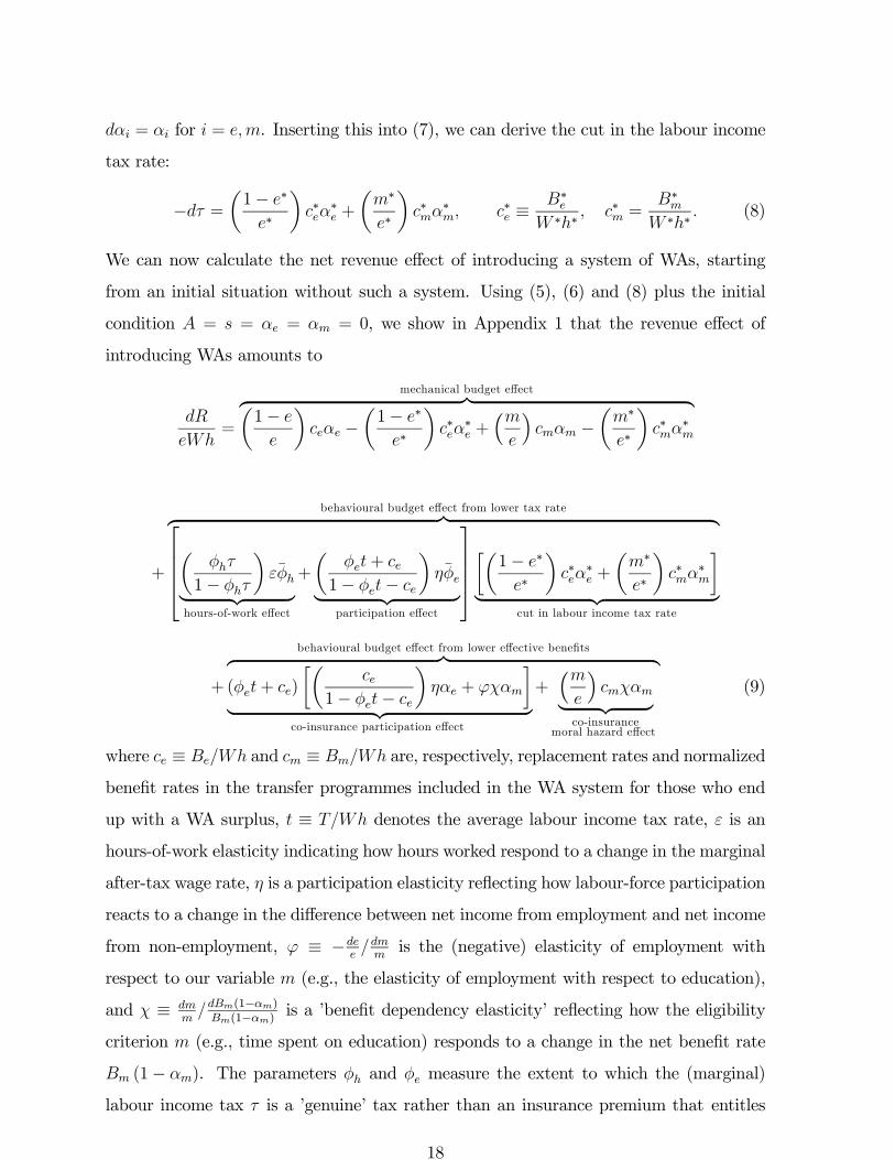
We can now calculate the net revenue effect of introducing a system of WAs, starting

from an initial situation without such a system. Using (5), (6) and (8) plus the initial

condition = = = = 0, we show in Appendix 1 that the revenue effect of

introducing WAs amounts to

=

mechanical budget effectz }| {µ1−

¶ −

µ1− ∗

∗

¶∗

∗ +

³

´ −

µ∗

∗

¶∗

∗

+

behavioural budget effect from lower tax ratez }| {⎡⎢⎢⎢⎣µ

1−

¶| {z }

hours-of-work effect

+

µ+

1− −

¶| {z }

participation effect

⎤⎥⎥⎥⎦∙µ1− ∗

∗

¶∗

∗ +

µ∗

∗

¶∗

∗

¸| {z }

cut in labour income tax rate

+

behavioural budget effect from lower effective benefitsz }| {(+ )

∙µ

1− −

¶ +

¸| {z }

co-insurance participation effect

+³

´| {z }

co-insurancemoral hazard effect

(9)

where ≡ and ≡ are, respectively, replacement rates and normalized

benefit rates in the transfer programmes included in the WA system for those who end

up with a WA surplus, ≡ denotes the average labour income tax rate, is an

hours-of-work elasticity indicating how hours worked respond to a change in the marginal

after-tax wage rate, is a participation elasticity reflecting how labour-force participation

reacts to a change in the difference between net income from employment and net income

from non-employment, ≡ −is the (negative) elasticity of employment with

respect to our variable (e.g., the elasticity of employment with respect to education),

and ≡ (1−)(1−) is a ’benefit dependency elasticity’ reflecting how the eligibility

criterion (e.g., time spent on education) responds to a change in the net benefit rate

(1− ). The parameters and measure the extent to which the (marginal)

labour income tax is a ’genuine’ tax rather than an insurance premium that entitles

18

the taxpayer to additional social insurance benefits. Under a pure Bismarckian social

insurance system with an actuarially fair link between social security taxes paid and

benefits received, we would have = = 0. At the opposite end of the spectrum, under

a pure Beveridgean social insurance system with no link between taxes and benefits at

the individual taxpayer level, we have = = 1. The parameters and in (9) are

defined as ≡ () and ≡ () , thus measuring the degree to which the

marginal effective tax rates and vary with the statutory marginal labour-income

tax rate These parameters may depend on the programmes that are included in the

welfare accounts.

3.2. Interpreting the formula

The ’mechanical’ budget effect indicated in (9) is the sum total of the positive WA bal-

ances that the government would have to transfer to the account holders if they would

not change their behaviour. Since these resources were previously part of general govern-

ment revenue, they measure the deterioration of the public budget in the hypothetical

situation where no taxpayer responds to the change in incentives brought about by the

WA system. In the absence of behavioral changes, the welfare accounts would thus not be

Pareto improving in an ex-post sense, since individuals without positive account balances

would lose (as the government would have to raise taxes to make up for its revenue loss).

Formula (9) reveals that the static revenue loss is larger, the more heterogeneous is the

population. In particular, the larger is the employment rate and the smaller are the av-

erage replacement rate and the call on non-employment benefits () for individuals with

positive WA balances relative to the population as a whole, the larger will be the positive

WA balance accruing to an average person within the group with positive balances, and

so the larger will be the revenue loss that occurs in the absence of behavioural responses.

Intuitively, with a more heterogeneous population, a conventional tax-transfer system

tends to imply more interpersonal redistribution from the lifetime rich to the lifetime

poor, so the larger is the static budgetary cost of reducing net revenue collection from

those individuals who are net taxpayers over the life cycle under the current system. One

can also interpret the static revenue loss as the distributional loss from the introduc-

tion of welfare accounts. This distributional loss is translated into a revenue loss, as the

19

government compensates those who end up losing from the accounts.

However, the introduction of WAs and the associated cut in the labour income tax will

affect labour-force participation, hours worked, and the take-up of social benefits, and

these behavioural responses will generate the ’behavioural’ budgetary effects indicated

in (9). The second line in (9) reflects the impact of a closer actuarial link between

contributions and benefits. This produces lower effective marginal and average tax rates,

resulting in more hours worked and more labour-force participation. The ’co-insurance

participation effect’ in the third line in (9) reflects that, via the WA system, consumers

partly self-finance the social benefits they receive during periods of non-employment. This

also induces them to reduce their periods of non-employment, thereby strengthening the

public finances. How much this participation effect improves the budget depends on the

initial overall tax and benefit wedge on employment + (the ’participation tax rate’)

and the sensitivity of inactivity with respect to a higher value of , as indicated by the

participation elasticity in formula (9).11

The (partial) self-financing of benefits via the WAs may also reduce the extent to

which citizens take up certain benefits that are not directly related to non-employment.

This is captured by the ’co-insurance moral hazard effect’ in the third line of equation (9).

When the benefit is not employment-related (e.g. child benefits), the co-insurance effect

does not directly affect employment. However, co-insurance may combat moral hazard in

other domains. In the case of child benefits, for example, fertility may decline if parents

have to pay the child benefits out of their own accounts. The resulting net revenue

effect depends on the product of a behavioural elasticity and a ’benefit wedge’¡

¢

indicating to what extent one child less saves the government money at the margin.

Similarly, if people have to pay their education benefits out of their own accounts, they

11We have included only labour-supply effects of lower effective replacement rates in our elasticity .

However, a lower effective replacement rate on account of a higher value for is also likely to reduce

wage pressure, thereby boosting labour demand and thus reducing the natural rate of unemployment

and benefit dependency. The lower effective tax rates produced by a closer actuarial link between

contributions and benefits may also reduce unemployment and thus stimulate employment through this

channel. To illustrate, Daveri and Tabellini (2000) find that the rise of 10 percentage points in the rate

of effective labour tax in continental Europe in the seventies and eighties can explain about 3 percentage

points of the increase in European unemployment during this period. Nickell and Layard (1999) estimate

an unemployment effect of about 2 percentage points of such a tax increase.

20

may take less education. The direct budgetary implications of less education are also

captured by the term¡

¢ in formula (9).

In addition, education benefits may generate an indirect budgetary effect since people

may move earlier to employment when they spend less time on education and/or since

they may retire earlier when lower education reduces their earnings potential. In these

cases we would have ≡ −6= 0. To the extent that child benefits affect fertility,

they may also have an indirect effect on employment as parents temporarily withdraw

from the labour market to rear their children (implying 0). The net revenue impli-

cations of these cross effects on participation are picked up by the term (+ )

included in the ’co-insurance participation effect’ in (9).

The decomposition of the budgetary impact in formula (9) in a mechanical and a

behavioural revenue effect allows a quantification of (some of) the efficiency gains from

the introduction of WAs. The behavioural revenue effect generated by the labour-supply

response to the reform is roughly equal to the increase in labour supply times the tax and

benefit wedge between the marginal productivity of labour and the marginal disutility of

work. To a first-order approximation, this behavioural revenue gain reflects the efficiency

gain from the increase in labour supply. It is given by the sum of the terms involving

the labour-supply elasticities , and in formula (9). The further revenue gain from

reduced moral hazard — represented by the term¡

¢ in (9) — also implies a welfare

gain, since the higher revenue allows the government to make (some) citizens better off.

However, in the presence of non-fiscal external effects, the overall welfare effect is com-

prised of more terms than the dynamic revenue effects alone. To illustrate, if (higher)

education produces a positive non-fiscal externality amounting to per student, where

is measured as a fraction of the pre-tax labour income of the representative worker

with a WA surplus, the fiscal external effects of a fall in the volume of education should

be amended by the non-fiscal external effect, − ¡

¢ to capture the overall welfare

effect. If education benefits are Pigovian so that the benefit rate is set equal to the non-

fiscal and fiscal external effect of education, we would have¡

¢ =

¡

¢− (+ ).

In that case, the terms involving the benefit dependency elasticity in (9) would drop out

from the expression for the welfare effect of including education benefits in the WA sys-

tem. Similarly, if fertility produces positive non-fiscal external effects and child benefits

21

are Pigovian, the terms including the elasticity should be neglected in the evaluation

of the welfare effect of including child benefits in the WA reform. In the analysis be-

low we assume that the benefits captured by our variable in (9) are indeed at their

Pigouvian levels. This enables us to ignore the terms that include the elasticities and

about which little is known. The assumption that the non-fiscal externalities have been

internalized also guarantees that the net effect of the WA reform on the public budget —

calculated by setting = = 0 — does in fact fully capture the net welfare effect of the

reform.

4. How would welfare accounts work in practice? An empirical

case study

To illustrate how formula (9) may be used to evaluate the likelihood that a switch to

individual accounts will generate a Pareto improvement, we now consider a specific WA

reform proposal for Denmark. There are four reasons why the introduction of WAs

is likely to improve the equity-efficiency trade-off in a country like Denmark. First, the

Danish system of social insurance is of the Beveridgean type, with almost no link between

taxes paid and benefits received. The bulk of social-insurance benefits is financed out of

general tax revenues, and most benefits are paid out in flat rates unrelated to previous

wages. Hence, the existing labour income taxes financing intrapersonal redistribution

over the life cycle incorporate a large distortionary element (in terms of formula (9), the

parameters and are close to one). Second, by international standards the effective

tax and benefit rates tend to be high in Denmark, so the efficiency gains from cuts in

these effective rates are potentially large. Third, as documented in Bovenberg, Hansen

and Sørensen (2008), the current Danish welfare state arrangements involve a very large

element of intrapersonal redistribution over the individual taxpayer’s life cycle. Finally,

compared to other countries, heterogeneity in gross (i.e. before-tax) lifetime incomes is

only limited in Denmark. As noted in the previous section, with a limited degree of

heterogeneity, the mechanical revenue loss from introducing WAs with a lifetime income

gurantee will be relatively small.

In the following, we describe theWA reform proposal and its mechanical impact on the

distribution of lifetime incomes. We then proceed to estimate its revenue and efficiency

22

effects by means of formula (9).

4.1. Illustration: A WA reform proposal for Denmark

The proposal we consider was originally presented in a report from the Danish Economic

Council (2005, ch. VI).12 According to the proposal, the individual welfare accounts

would respect principles 1) through 8) explained in section 2.2. As noted, these prin-

ciples guarantee a Pareto improvement as long as the WA reform improves the public

budget. When selecting the transfer programs to be included in the WA system, the

Danish Economic Council (DEC) focused on those programs involving the lowest degree

of interpersonal redistribution in order to minimize the potential negative impacts on

lifetime income distribution. Specifically, the DEC proposed that the following transfers

should be debited to the recipient’s individual WA:

1. Early retirement benefits

2. Grants to students in higher education

3. Short-term unemployment benefits

(for unemployment spells up to a length of three months)

4. Short-term sickness benefits (up to a limited number of sickness days)

5. Child benefits (universal child benefits paid to all parents)

6. Parental leave benefits

As we saw in Table 1, all of these Danish transfer programs imply a relatively low

amount of redistribution of lifetime incomes. In terms of our formula (9), the magnitudes¡1−

¢−

¡1−∗∗¢∗

∗ and

¡

¢−

¡∗∗¢∗

∗ for these programmes therefore tend

to be relatively small, so including only these programmes in the WA system helps to

minimize the mechanical revenue loss. According to the data underlying Table 1, the

degree of lifetime income redistribution achieved by benefits paid to workers suffering

long unemployment spells (exceeding three months) is more than twice as large as the

interpersonal redistribution generated by short-term unemployment benefits (for spells

12Established by the Danish parliament in 1962, the Economic Council is an independent think tank

advising the Danish government and parliament on issues of economic policy. The WA proposal con-

sidered here was developed while Peter Birch Sørensen was chairing the council and Martin Ino Hansen

was working for the council secretariat.

23

shorter than three months). For this reason, the DEC proposed that if a person has been

unemployed for more than three months, only the benefits collected during the first three

months should be debited to his/her WA. Similarly, benefits paid during long sickness

spells tend to be more redistributive than benefits paid during short spells. Moreover,

short-term sickness spells tend to involve a greater moral hazard problem of verifiability.

The DEC therefore proposed that only benefits paid during a limited number of sickness

days from the start of the sickness spell should be included in the WA system. However,

data limitations compelled us to include all sickness benefits in the calculations presented

below.

The DEC proposed that the mandatory contributions to the WAs should be propor-

tional to the base for the Danish payroll tax (which is also levied on an imputed labour

income for the self-employed) and that the existing proportional payroll tax should be

reduced by a corresponding amount. This is in line with our previous assumption that

= −. It was also proposed that the contribution rate should be set so that the ag-gregate contributions to the WAs would equal the aggregate benefits collected under the

programmes included in the system, assuming unchanged behaviour. This corresponds

to our assumption in (7), which was used to derive our formula (9) for the budgetary

effects.

Table 3 shows the DEC’s estimate of the impact of the proposed WA system on the

distribution of lifetime incomes, assuming a zero growth-adjusted real after-tax interest

rate. Importantly, the table abstracts from any behavioural effects of theWA system. The

numbers thus reflect only the mechanical budgetary effect. Although the very purpose

of the WA system is to influence behaviour, the distribution of positive WA balances in

Table 3 should provide a good proxy for the effect of the reform on the distribution of

individual welfare. The reason is that, by the Envelope Theorem, behavioural changes

caused by the WA system yield no first-order effects on individual welfare if individuals

have optimized their behaviour in the initial equilibrium and are not rationed on the

labour market.13

13The WAs do not have first-order implications for the welfare impact of capital-market imperfections

such as liquidity constraints. The reason is that the WAs allow individuals to enjoy the same insurance

benefits as under the current system — even if their account balance is negative. In this respect, the

accounts provide the same liquidity insurance as current public benefits.

24

(Table 3 about here)

The second row in Table 3 shows the accumulated contributions to the WA relative

to the accumulated withdrawals from the account for each of the deciles in the lifetime

income distribution. Not surprisingly, this ratio rises systematically with lifetime income.

Moreover, the ratio of the average positive WA balance to lifetime income is also rising

with the income level, as shown in the third row in Table 3. Furthermore, whereas only

7.2 percent of individuals in the lowest decile end up with a positive WA balance at the

time of retirement (assuming unchanged behaviour), almost 80 percent of people in the

top decile will accumulate a positive balance, as indicated in the fourth row of the table.

This distributional pattern reflects the fact that the contributions to the WA are

proportional to labour income whereas most of the benefits included in the WA system

are paid out in flat rates. Moreover, people who are less active in the labour market

and more dependent on the transfer system tend to end up in the lower lifetime income

brackets. There is thus no doubt that the DEC proposal for a WA system will make

the lifetime income distribution more unequal. The distributional impact will be limited,

however. Specifically, while the Gini coefficient for the distribution of disposable lifetime

income is 0.127 under the current Danish tax-transfer system, it would rise only to 0.133 if

the proposed WA system were introduced (Danish Economic Council, 2005, ch. VI). The

Gini coefficient for the distribution of lifetime market income is currently 0.253. While

the redistribution of lifetime income implied by the current tax-transfer system amounts

to (0.253-0.127)/0.253 = 49.8 percent, the redistribution under the DEC proposal would

thus still amount to a substantial (0.253-0.133)/0.253 = 47.4 percent.14 Moreover, and

most importantly, it is possible to redistribute the efficiency gains from the WA reform

so as to neutralize the tendency towards higher inequality, as we shall explain in section

5.

4.2. Effects on the public budget and on economic efficiency

We now employ formula (9) to estimate the revenue and welfare effects of the DEC

proposal. The formula requires a distinction between those benefits in the WA system

14These mechanical calculations are based on the heroic assumption that factor incomes are unaffected

by the tax-transfer system.

25

that are directly related to the recipient’s employment status and those that are not. In

the latter category we include (universal) child benefits and benefits to students in higher

education, whereas unemployment benefits, sickness benefits, early retirement benefits

and parental leave benefits are clearly paid out only during periods of non-employment.

The data on disposable lifetime incomes underlying Table 3 include estimates of the

various transfers received by individuals over their working lives. From these estimates

we have calculated the magnitudes ¡1−

¢ ∗

∗

¡1−∗∗¢

¡

¢and ∗

∗

¡∗∗¢

appearing in our formula (9) — that is, the average amount of after-tax benefits withdrawn

from the WA relative to average pre-tax income for individuals with a WA surplus and for

the population as a whole, respectively. As explained above, the difference between these

magnitudes determines the size of the mechanical revenue loss from a WA system, before

accounting for the budgetary impact of behavioural changes. The first column in Table

4 shows our estimates of ∗∗

¡1−∗∗¢and ∗

∗

¡∗∗¢, while the second column presents

our estimates of ¡1−

¢and

¡

¢. The differences in these magnitudes between

people with a WA surplus and the population as a whole depend in part on the size of the

transfer program and partly on the skewness of the distribution of the benefits from the

program. The differences between the numbers in the first and second columns in Table 4

- i.e., the mechanical revenue effects - depend also on the specific transfers included in the

WA system, because this will determine the separation between people with and without

a WA surplus. Furthermore, recall from equation (9) that the magnitudes ∗∗

¡1−∗∗¢and

∗∗

¡∗∗¢in the first column of Table 4 indicate the proportional cut in the effective

(direct and indirect) labour income tax rate made possible by including the relevant

transfer program in the WA system.

To estimate the co-insurance participation effects captured by the bottom line of

formula (9), we also need estimates for and i.e. the fraction of total transfers

to people of working age accounted for by the various transfer programs included in the

WA system. For each particular transfer program included in the account system we

have = 1. However, the parameter in our formula (9) measures the fraction of total

transfers to non-employed people of working age (who end up with a WA surplus) that is

included in the WA system. To estimate how much, say, the inclusion of early retirement

benefits contributes to , we may therefore divide the number in the first row and

26

second column of Table 4 by the figure in the seventh row and second column, obtaining

a contribution to equal to 116283 = 0411. In other words, early retirement benefits

amount to about 41 percent of the total transfers to those individuals of working age

who end up with a surplus on their WA, as indicated by the figure in the top row and

last column of Table 4. The contributions to of the other transfer programmes for

non-employed individuals are found in a similar way, and by summing the contributions

from the four programmes included included in the WA system, we obtain = 0672,

implying that for people with a WA surplus roughly two thirds of the out-of-work benefits

they receive during their careers are drawn from their welfare accounts. In the same way

we find that = 0928, i.e. almost 93 percent of the benefits that are not related to

employment status are drawn from the WAs of those with an account surplus, as shown

in the 11th row and last column of Table 4.

(Table 4 about here)

When applying formula (9), it must be recalled that the effective tax rates on labour

income include indirect taxes; therefore, prior to the adjustment for a possible link be-

tween taxes and benefits, the effective marginal and average tax rates on labour income

are given as

= +

1 + =

+

1 + (10)

where and denote the marginal and average direct tax rates, respectively, and

stands for the overall effective indirect tax rate on consumption. In Denmark, realistic

values of these tax parameters for an average worker would be15

= 054 = 042 = 026 =⇒ = 063 = 054

Application of formula (9) also requires an estimate of our parameters and

quantifying the degree to which increases in employment and hours worked generate

additional benefit rights. Suppose the benefit rate obtainable in some transfer programme

15The estimate for is taken from the OECD Taxing Wages report (OECD (2005)) and refers to the

average Danish production worker. The estimate for the average value of the marginal direct tax rate

on labour income () is taken from the Danish Ministry of Finance (2004), and the estimate for is

based on Carey and Rabesona (2004, Table 7.B2) and is an average figure for Denmark for the period

1990-2000.

27

depends on previous earnings. In that case a unit increase in earnings today will increase

the future net benefit rate by the replacement rate . Suppose further that on average the

wage earner expects to be eligible for the benefit during some fraction of his remaining

labour-market career. With a zero growth-adjusted discount rate, this person’s effective

tax rate on labour income should then be reduced by the amount because additional

earnings generate additional future benefits. However, for some people eligible for the

benefit, the benefit rate may be unrelated to previous earnings — for example, because

benefits are capped. Hence, we estimate our parameters and by the simple formulas

= − = − (11)

where is the fraction of workers who are in a position to raise their future benefits

by increasing their current working hours, and is the fraction of people in the work-

force who can increase their future benefit rights by moving from non-employment into

employment. Note that the parameters , , and are averages across all transfer

programmes for those individuals of working age who (expect to) end up with a surplus

on their WA. In Appendix 2 we explain in detail how we have arrived at the estimates

≈ = 02, = 017 and = 025 to find

= 0992 = 0991

These estimates reflect the very low degree of actuarial fairness of the Danish system of

social insurance.

Although estimates of the average (uncompensated) wage elasticity of hours worked

for Denmark tend to centre around 0.1 (a little higher for females and a little lower

for males; see Frederiksen et al. (2001)), we select = 005 to be on the conservative

side. The participation elasticity was estimated by Le Maire and Scheuer (2005) to

be in the range 0.2-0.4 for Danish recipients of social assistance benefits. However, for

high-wage earners who are rarely in need of social assistance benefits, the participation

elasticity is likely to be somewhat lower, so we conservatively set = 01. By selecting

low values for the labour-supply elasticities, we account for the possibility that some

agents may be myopic or liquidity-constrained and therefore do not fully take account

of the intertemporal links between withdrawals from the accounts and future retirement

benefits.

28

Finally, since we assume that education benefits and child benefits are set at their

Pigovian levels, we can abstract from the ’co-insurance’ terms involving the parameters

and in formula (9), as we explained earlier. Inserting our assumptions on parame-

ter values plus the relevant data from Table 4 into (29), we then obtain the estimated

budgetary effects stated in Table 5.

(Table 5 about here)

Given our assumed parameter values, we see that the proposed WA system would

improve the public budget by more than six percent of the initial labour income tax base

for the group that ends up with an account surplus. According to the data underlying

Table 3, amounts to almost 60 percent of the total labour income tax base, so the

estimated gain in net revenue is about 3.75 percent of the total labour income tax base,

or roughly 212percent of GDP. Table 5 shows that the bulk of the dynamic net revenue

gain comes from the participation response to the cut in effective benefit rates implied

by the WA system (see column 4 in the table). This is not surprising, considering that

the WA system effectively cuts the replacement rate by 100 percent in those transfer

programs that are included in the system.

To illustrate the workings of the account system, it may be instructive to consider the

first row in Table 5, which shows the various effects of including short-term unemployment

benefits in the WA system. The inclusion of this program in the account system allows

a cut in the marginal effective labour income tax rate of about 1.18 percentage points,

as indicated in the fourth row and first column of Table 4. Multiplying this tax rate

cut by the factor³

1−

´ appearing in formula (9), we can estimate the rise in tax

revenue generated by the increase in working hours resulting from including short-term

unemployment benefits in the WA system. Clearly, this effect depends on the hours-of-

work elasticity and the initial level of the marginal effective labour income tax rate,

. Using the parameter values mentioned above, we estimate an increase in tax revenue

amounting to 0.1 percent of the labour income tax base (for individuals with a WA

surplus), as shown in the first row and second column of Table 5.16 The average tax rate

on labour income will also drop by 1.18 percentage points when short-term unemployment

16In applying formula (9), we use the facts that ≡ () = and ≡ () = .

29

benefits are included in the WA system because the Danish payroll tax (which is cut pari

passu with the rise in ) is purely proportional. This will stimulate labour supply at

the extensive margin, as the lower average tax burden on labour income induces the

unemployed to increase their search efforts in order to move faster into employment. The

resulting effect on the public budget is captured by the term³

+1−−

´ in formula

(9). This term includes the ’participation elasticity’ (in this case picking up the effect of

more intensive job search) and the initial effective ’participation tax rate’ + which

reflects the increased tax burden and the loss of after-tax benefit income experienced by

an individual who moves from unemployment into employment. Given our assumptions

on parameter values, we estimate that the cut in the average effective labour income tax

rate increases the employment rate by about 0.54 percent. This will in turn improve the

budget by 0.42 percent of the labour income tax base, as reported in the first row and

third column of Table 5.

Finally, since collection of short-term unemployment benefits reduces a worker’s WA

balance by a similar amount in present value terms, the inclusion of these benefits in

the WA system provides a further strong incentive for forward-looking individuals to

raise their labour supply at the extensive margin through increased search effort. The

resulting effect on the budget is reflected in the term (+ )³

1−−

´ in formula

(9), where the estimate for is found from Table 4 in the manner explained earlier. On

this basis, we obtain a budgetary improvement of 1.66 percent of the labour income tax

base, as stated in the first row and fourth column of Table 5. The total dynamic effect

on the budget is the sum of the three effects just mentioned, adding up to 2.19 percent

of the labour income tax base of individuals with a positive WA balance (who account

for 60 percent of the total labour income tax base).

As mentioned, our estimates in Table 5 do not include the direct effects on labour

force participation of incorporating education benefits and child benefits in the WA sys-

tem, since we assume that the resulting fiscal externalities are offset by changes in the

non-fiscal external effects associated with education and child-bearing. Under this as-

sumption, and provided there are no non-fiscal externalities associated with the other

transfer programmes, the behavioural revenue gain is a proxy for the welfare gain from

the introduction of WAs, as we explained in section 4. From column 5 in Table 5, this

30

efficiency gain for the WA system as a whole can be estimated to amount to a respectable

4.9 percent of the total labour income tax base (06 · 814 ≈ 49) or roughly 3.3 percentof GDP. Note that since the proposed WA system ensures that nobody can be finan-

cially worse off than under the existing tax-transfer system, the estimated efficiency gain

represents a genuine ex-post Pareto improvement. One might argue that the parental

leave scheme has a positive external effect insofar as parental care in the early stage of

childhood improves the social skills of the child. If there are negative non-fiscal external-

ities associated with non-employment (e.g., increased crime rates and loss of self-respect

and social skills), however, the increase in employment obtained through the WA system

would have positive external effects that are not included in Table 5. It is thus not at all

obvious that an allowance for non-fiscal externalities would reduce the estimated total

welfare gain. At any rate, the estimate in the bottom row and fifth column of Table 5

shows how large the possible loss in non-fiscal externalities would have to be to eliminate

the total net welfare gain from the WA system.

4.3. Sensitivity analysis

The size of the parameters determining the effects of the WA system on the public

budget is uncertain. Table 6 therefore investigates how sensitive the budget effects and

the efficiency effects are to changes in some key parameters.

(Table 6 about here)

The first row in the table restates the estimates of the total efficiency and revenue

effects from our benchmark scenario in Table 5, using the behavioural budget effect as a

proxy for the efficiency effect. In the benchmark scenario we assumed (based on estimates

laid out in Appendix 2) that only about 20 percent of the Danish workforce are in a posi-

tion where they can increase their benefit entitlements by increasing their labour supply.

In terms of the formulas in (11), this means that = = 02. To check the importance

of the values of these parameters, the second row of Table 6 assumes counterfactually

that all workers can raise their entitlements to social transfers by increasing their labour

force participation and by working more hours, i.e., = = 1. The benefit system will

then work as a stronger offset to the tax-induced distortions to labour supply, thereby

31

reducing the size of the initial effective tax wedges. Not surprisingly, we see from the

second row of Table 6 that this reduces the size of the revenue and efficiency gain from

the WA reform, but we also see that sizeable gains remain.

Our benchmark scenario assumed that, for people already employed, the elasticity of

hours worked (or more broadly, the elasticity of taxable income at the intensive margin

of labour supply) with respect to the effective marginal after-tax wage rate takes a rather

low average value of 0.05. It would not be unreasonable to assume a higher value of this

elasticity such as = 01. From the third row in Table 6 we see that this would increase

the efficiency and revenue gains from the WA system, although not dramatically so.

These examples indicate that the exact values of the parameters , and are not

very important for our conclusion that the introduction of WAs is likely to generate a

Pareto improvement. The last two rows in Table 6 suggest that the elasticity of labour

force participation with respect to the net gain from employment () is more important

for the size of the welfare gain. Our benchmark scenario assumed an average participation

elasticity of 0.1. Table 6 shows that if this elasticity is only half as high ( = 005), the

efficiency gain from the reform is almost cut in half, and the net revenue gain is more than

halved. Still, a respectable revenue gain will remain — even with such a low participation

elasticity. On the other hand, if = 015, we see that the aggregate efficiency gain from

the reform would be around 12 percent of the pre-tax earnings of people with a WA

surplus, and the net revenue gain would amount to about 10 percent of those earnings.

The great importance of the participation elasticity reflects the fact that, whereas the

WA system only allows a limited fall in effective marginal tax rates, it implies that the

effective replacement rates in the transfer programmes included in the system are cut

to zero. The labour-supply response to this dramatic cut takes place at the extensive

margin where people decide to move from non-employment into employment, and the

magnitude of this response is reflected in the participation elasticity.

Overall, the numerical exercises in this section strongly suggest that, at least in

the context of the Danish tax-transfer system, the introduction of welfare accounts for

those transfer programs that involve relatively little interpersonal redistribution would

be Pareto-improving, provided the WA system includes a ’lifetime income guarantee’ (a

bail-out clause) for those who end up with a negative account balance.

32

5. Redistributing the gains from welfare accounts

The reform proposal discussed above was designed to illustrate in a simple example how

a WA system may generate a Pareto improvement. However, the proposal does raise

some issues of horizontal and vertical equity.

The horizontal equity issue may also be seen as an issue of lost insurance. For example,

suppose persons A and B have the same lifetime labour income and that they are both

able to accumulate a surplus on their welfare account, but that B is more frequently ill.

Person B would then end up with a lower WA surplus than A, since the proposed WA

system implies that people with an account surplus self-insure against short-term spells of

illness. By contrast, under the current (Danish) tax-transfer system all sickness benefits

are financed out of general tax revenues. On the other hand, since B is assumed to have

the same lifetime income as A despite being more frequently out of work, B must have a

higher earnings capacity than A. One might therefore argue that B is in a better position

to self-insure against social contingencies. At any rate, the lifetime income guarantee

ensures that no person suffering frequent spells of sickness, unemployment etc. can be

worse off under the WA system than under the present system.

The issue of vertical equity is illustrated by Table 3, which shows that there is a clear

tendency for the frequency and size of the WA surplus to rise with the level of income.

Although we saw earlier that the impact on lifetime income distribution would be limited,

it is thus indisputable that the gains from the WA system described in the previous

section would accrue mainly to high-income earners. This might be seen as undesirable,

especially since the income distribution in many countries has already become more

unequal in recent decades.

However, since the WA reform improves the equity-efficiency trade-off, it allows the

government to improve social welfare even if policy-makers choose to redistribute some

of the gains from the reform towards low-income earners. For example, the government

could choose to raise out-of-work benefits, financed by some appropriate combination of

a higher mandatory contribution to the WA, a higher marginal tax rate on high-income

earners (thereby clawing back part of the tax cut made possible by the WA reform)

and the revenue gain from the WA reform. Such a policy would redistribute lifetime

income towards low-income earners who end up with a WA deficit. At the same time,

33

the higher benefits would not weaken the work incentives of people with a WA surplus

since these persons finance their own benefits via their individual WA accounts. Indeed,

Bovenberg and Sørensen (2004) show that under the WA system, the efficiency cost of

raising the out-of-work benefits is lower than under a conventional tax-transfer system

because the higher benefits weaken the incentives only of individuals who do not expect

to accumulate a WA surplus. With a lower efficiency cost of redistribution, a government

seeking the optimal balance between equity and efficiency would want to undertake more

redistribution.

If policy-makers do not wish to weaken the work incentives of low-income earners by

raising benefits, there are other ways of redistributing the gains from the WA system.

For example, the ’default line’ in the system could be moved below zero. This would

mean that, instead of paying out a supplement to the public pension only when the

final account balance is positive, the additional pension would be equal to the amount

by which the WA balance exceeds a certain negative threshold. Thus, only people with

negative WA balances below a certain level would be affected by the bail-out clause. This

would increase the number of people who would benefit from the WA system and who

would be affected by the stronger work incentives implied by the system.

Another amendment to the WA system that would tend to redistribute the gains

towards unlucky individuals (many of whom would end up with low lifetime incomes)

would be to set a ’debt limit’ to the negative balance that can be accumulated on the

WA, as proposed by Fölster (1999). When net withdrawals from the account exceed a

certain limit, the account holder would still be able to collect benefits under the standard

eligibility rules, but these benefits would no longer be debited to his/her WA. This would

increase the chance that even unlucky individuals with large benefit needs would be able

to accumulate a WA surplus.

Of course, the government would have to find ways of financing the additional pensions

paid out from the WAs. As we have seen, the account system is likely to improve the

public budget, so this could provide part of the financing. To enhance the redistributive

profile, another part of the financing could come from a higher marginal tax rate on

high-income earners or from a progressive tax on positive WA account balances. Clearly,

the two latter modes of financing would imply a smaller improvement of the incentives

34

of high-income earners, but overall the WA system would still provide stronger work

incentives than the present tax-transfer system.

6. Concluding remarks

This paper has argued that individual welfare accounts can play a useful role in financing

social benefits that have only little redistributive power in a life-cycle perspective and

that give rise to serious moral hazard. We believe that several recent economic, social

and technological trends combine to make individual accounts in social insurance more

attractive.

First of all, changes in technology and in the organisation of work have made many

segments of the labour market more ’fluid’, as people move more frequently between

employers and as they enter and exit the labour force more often. In such a transitional

labour market, it becomes more difficult to verify whether a person is voluntarily or in-

voluntarily out of work. Furthermore, as the economy shifts from blue-collar work in

industrial sectors to white-collar work in service sectors and knowledge-intensive activi-

ties, mental causes of sickness become more prominent. These types of sickness are less

easy to diagnose and verify than those with physical causes. All of these labour market

trends tend to increase the danger of moral hazard in social insurance. A WA system

would counteract the growing risk of moral hazard.

Second, modern information and communication technologies enable governments to

keep systematic records of the social security taxes paid and the benefits received by

individual citizens over their working careers. This should facilitate the administration

of welfare accounts.

Third, liberalized capital markets allow individuals to smooth their consumption over

their life courses. By thus enabling individuals to decouple annual consumption from an-

nual disposable incomes, better functioning capital markets make lifetime incomes rather

than annual incomes better indicators of overall welfare. This increases the relevance of

the WA system in which redistribution is based on lifetime income rather than annual

income.

A further reason for the increased attractiveness of individual accounts is that they

are fully portable between jobs. Hence, social insurance does not tie workers to their

35

initial employer. This facilitates labour mobility and the flexibility of the labour mar-

ket. Finally, many social-insurance programs suffer from the problem that it is hard to

separate the truly needy from other individuals who do not really need help from the

government. If social norms regarding the take-up of benefits are endogenous and the

take-up rate depends positively on how many people already receive benefits (as argued

by Lindbeck (2006)), individual accounts may improve the sustainability of the welfare

state by inducing people not to take up social benefits unless they really need them. This

helps to halt an erosion of social norms. With individual accounts reducing moral haz-

ard for middle- and higher incomes, the government can focus its active labour-market

policies more on the lifetime poor, thereby also protecting the social norms of this group.

APPENDIX 1

This appendix shows how to derive formula (9) presented in section 3 and used in

section 4 to estimate the effects on the public budget of introducing individual accounts.

The introduction of WAs involves a cut in combined with a rise in the variables ,

and from zero to some positive numbers. Using equations (5) and (6) in section

3;17 remembering that = = = 0 initially; and recalling that the proposed WA

system does not involve any change in ordinary retirement benefits (i.e., = 0), we find

17Equation (5) assumes that contributions to the WA are not deductible, that WA balances are not

taxed, and that only net (after-tax) benefits are debited to the WA. Alternatively, one may assume that

pre-tax benefits are debited to the WA and that WA contributions are deductible from the personal

income tax base whereas WA balances are subject to tax. In this case, by using = − , one can

show that (5) modifies to

= − (1− ) (1− ) − (1− )−

+¡ −

¢+

µ −

1−

¶[ (1− ) + ] (i)

where is the average tax rate on WA balances, and is the average tax rate on benefit income. How-

ever, in the initial pre-reform equilibrium we have = = = 0, so to a first-order approximation,

changes in and will have no impact on via the last two terms on the right-hand side of (i). Hence,

an analysis based on (5) still approximates the revenue effect of the reform.

36

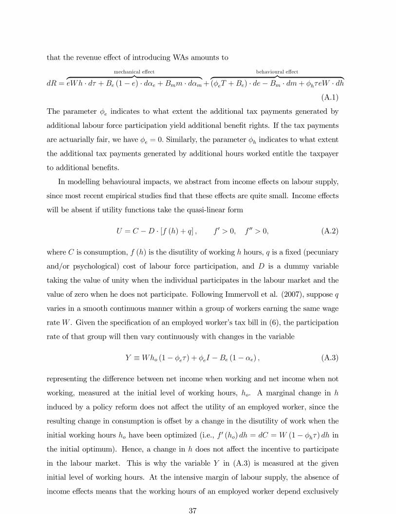
that the revenue effect of introducing WAs amounts to

=

mechanical effectz }| { · + (1− ) · + · +

behavioural effectz }| {( +) · − · + ·

(A.1)

The parameter indicates to what extent the additional tax payments generated by

additional labour force participation yield additional benefit rights. If the tax payments

are actuarially fair, we have = 0 Similarly, the parameter indicates to what extent

the additional tax payments generated by additional hours worked entitle the taxpayer

to additional benefits.

In modelling behavioural impacts, we abstract from income effects on labour supply,

since most recent empirical studies find that these effects are quite small. Income effects

will be absent if utility functions take the quasi-linear form

= − · [ () + ] 0 0 00 0 (A.2)

where is consumption, () is the disutility of working hours, is a fixed (pecuniary

and/or psychological) cost of labour force participation, and is a dummy variable

taking the value of unity when the individual participates in the labour market and the

value of zero when he does not participate. Following Immervoll et al. (2007), suppose

varies in a smooth continuous manner within a group of workers earning the same wage

rate . Given the specification of an employed worker’s tax bill in (6), the participation

rate of that group will then vary continuously with changes in the variable

≡ (1− ) + − (1− ) (A.3)

representing the difference between net income when working and net income when not

working, measured at the initial level of working hours, . A marginal change in

induced by a policy reform does not affect the utility of an employed worker, since the

resulting change in consumption is offset by a change in the disutility of work when the

initial working hours have been optimized (i.e., 0 () = = (1− ) in

the initial optimum). Hence, a change in does not affect the incentive to participate

in the labour market. This is why the variable in (A.3) is measured at the given

initial level of working hours. At the intensive margin of labour supply, the absence of

income effects means that the working hours of an employed worker depend exclusively

37

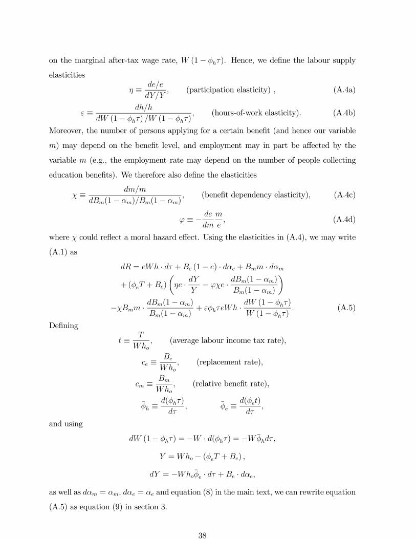
on the marginal after-tax wage rate, (1− ). Hence, we define the labour supply

elasticities

≡

(participation elasticity) , (A.4a)

≡

(1− ) (1− ) (hours-of-work elasticity). (A.4b)

Moreover, the number of persons applying for a certain benefit (and hence our variable

) may depend on the benefit level, and employment may in part be affected by the

variable (e.g., the employment rate may depend on the number of people collecting

education benefits). We therefore also define the elasticities

≡

(1− )(1− ) (benefit dependency elasticity), (A.4c)

≡ −

(A.4d)

where could reflect a moral hazard effect. Using the elasticities in (A.4), we may write

(A.1) as

= · + (1− ) · + ·

+( +)

µ ·

− · (1− )

(1− )

¶− · (1− )

(1− )+ · (1− )

(1− ) (A.5)

Defining

≡

(average labour income tax rate),

≡

(replacement rate),

≡

(relative benefit rate),

≡()

≡

()

and using

(1− ) = − · () = −

= − ( +)

= − · + ·

as well as = = and equation (8) in the main text, we can rewrite equation

(A.5) as equation (9) in section 3.

38

APPENDIX 2

This appendix explains how we estimated the parameters and quantifying the

degree to which increases in employment and hours worked generate additional benefit

rights. Since Danish public retirement benefits are unrelated to previous earnings, the

discussion below refers only to transfer programs for people of working age.

As explained in section 4 of the paper, the starting point is the formulas

= − = − (A.6)

where is the fraction of workers who are in a position to raise their future benefits by

increasing their current working hours, is the fraction of people in the workforce who

can increase their future benefit rights by moving from non-employment into employment,

is the average replacement rate (the after-tax benefit relative to pre-tax earnings), and

is the average non-employment rate. The parameters , and are averages

across all transfer programs for those individuals of working age who (expect to) end up

with a surplus on their welfare account.

In the Danish systems of unemployment insurance and sickness benefits, the benefit

rate does in principle vary in proportion to previous earnings, but there is a relatively low

cap on the benefit rates, implying that only about 10 percent of full-time workers actually

experience a direct link between their benefits and their previous wage income. However,

for some part-time workers a move from part-time to full-time employment may cause an

increase in the rates of unemployment and sickness benefits that they may collect if they

become unemployed or get sick. In recent years the share of Danish workers working less

than 30 hours per week has been slightly less than 9 percent. Persons working longer than

that will generally not obtain additional benefit rights by increasing their hours worked.

Against this background, we set = 02 to cover that fraction of the workforce where

a link between hours worked and future benefits received may reasonably be expected.

This estimate will tend to understate the existing tax distortions (and hence to stack the

deck against our WA proposal) because several transfer programs offer purely flat rates

of benefit with no link between benefits and earnings for any benefit recipient.

The replacement rate in (A.6) may be written as (1− ) , where is

the average pre-tax benefit paid to people out of work, and is the average effective tax

39

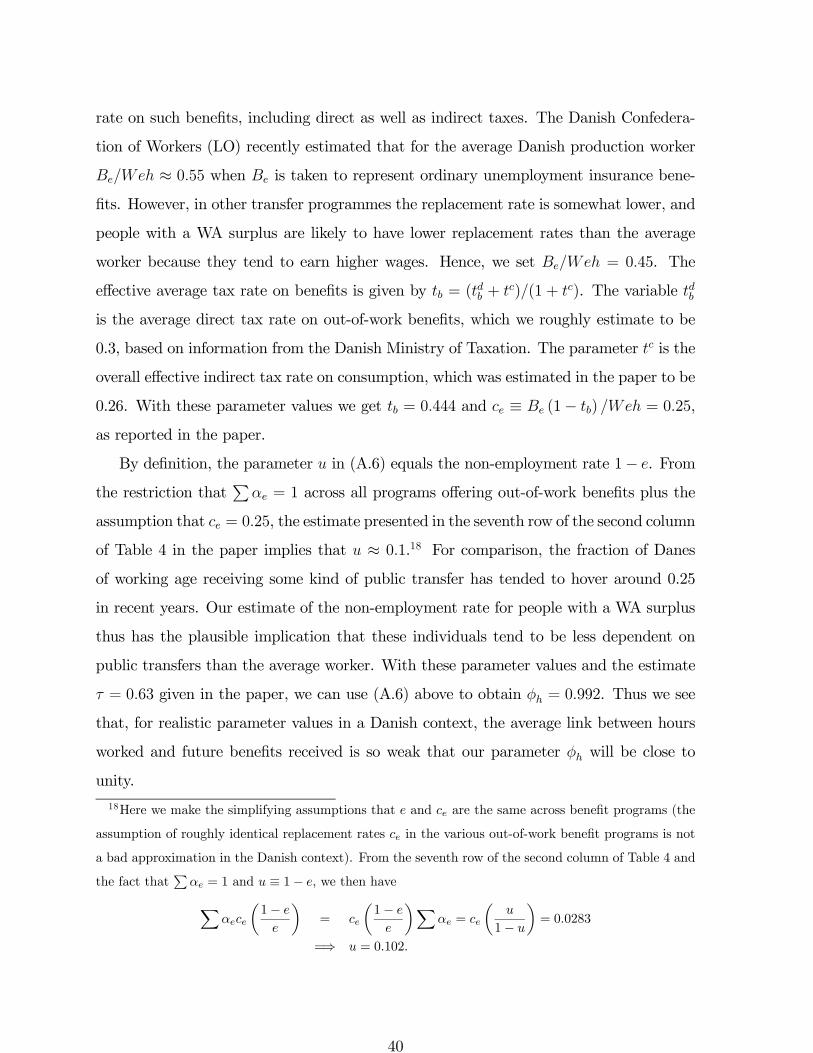
rate on such benefits, including direct as well as indirect taxes. The Danish Confedera-

tion of Workers (LO) recently estimated that for the average Danish production worker

≈ 055 when is taken to represent ordinary unemployment insurance bene-

fits. However, in other transfer programmes the replacement rate is somewhat lower, and

people with a WA surplus are likely to have lower replacement rates than the average

worker because they tend to earn higher wages. Hence, we set = 045. The

effective average tax rate on benefits is given by = ( + )(1 + ). The variable

is the average direct tax rate on out-of-work benefits, which we roughly estimate to be

0.3, based on information from the Danish Ministry of Taxation. The parameter is the

overall effective indirect tax rate on consumption, which was estimated in the paper to be

0.26. With these parameter values we get = 0444 and ≡ (1− ) = 025,

as reported in the paper.

By definition, the parameter in (A.6) equals the non-employment rate 1− . From

the restriction thatP

= 1 across all programs offering out-of-work benefits plus the

assumption that = 025, the estimate presented in the seventh row of the second column

of Table 4 in the paper implies that ≈ 01.18 For comparison, the fraction of Danesof working age receiving some kind of public transfer has tended to hover around 0.25

in recent years. Our estimate of the non-employment rate for people with a WA surplus

thus has the plausible implication that these individuals tend to be less dependent on

public transfers than the average worker. With these parameter values and the estimate

= 063 given in the paper, we can use (A.6) above to obtain = 0992. Thus we see

that, for realistic parameter values in a Danish context, the average link between hours

worked and future benefits received is so weak that our parameter will be close to

unity.

18Here we make the simplifying assumptions that and are the same across benefit programs (the

assumption of roughly identical replacement rates in the various out-of-work benefit programs is not

a bad approximation in the Danish context). From the seventh row of the second column of Table 4 and

the fact thatP

= 1 and ≡ 1− , we then haveX

µ1−

¶=

µ1−

¶X =

µ

1−

¶= 00283

=⇒ = 0102

40

We turn next to the estimation of from the formula = − where is

the fraction of people in the workforce who can increase their future benefit rights by

moving from non-employment into employment. In Denmark, a member of an unem-

ployment insurance scheme is entitled to unemployment insurance benefits if he/she has

been employed for at least one year during the latest three years. Uninsured workers are

entitled to a means-tested social assistance benefit in case of unemployment, provided

they are available for work. The benefit depends on the current income and wealth of the

household, but not on the previous earnings of the recipient. This means test may imply

that also the spouse faces a disincentive to participate in the labour market, thus tending

to increase rather than decrease our parameter . To be entitled to sickness benefits, a

person has to have been employed only during the previous 8 weeks. Entitlement to early

retirement benefits is obtained by 25 years of membership of an unemployment insurance

scheme. Most other transfer programs involve no link between employment and benefit

entitlement. Estimating the ’correct’ value of on the basis of these benefit eligibility

rules is quite difficult, but an upper bound on would certainly be given by the propor-

tion of Danes of working age (aged 18-65) who are non-employed. As already mentioned,

this fraction is roughly 25 percent, so fairly conservatively we insert = 02 along with

our earlier estimates = 054, = 01 and = 025 into the formula = −

to obtain = 0991. Again, we thus conclude that in the Danish labour market the

non-distortionary fraction of the labour income tax is very low indeed.

REFERENCES

Barr, N. and P.A. Diamond (2008). Reforming pensions: principles, analytical errors and

policy directions. International Social Security Review 62, 5-19.

Bovenberg, A.L. and P.B. Sørensen (2004). Improving the equity-efficiency trade-off:

Mandatory savings accounts for social insurance. International Tax and Public Finance

11, 507-529.

Bovenberg, A.L. and P.B. Sørensen (2007). Working to account: social security without

dependency. Politeia, London.

Bovenberg, A.L. M.I. Hansen and P.B. Sørensen (2008). Individual savings accounts for

social insurance: rationale and alternative designs. International Tax and Public Finance

41

15, 67-86.

Brown, A.J.G., J.M. Orszag and D.J. Snower, 2006, Unemployment accounts and em-

ployment incentives. Kiel Working Paper No. 1274.

Carey, D. and J. Rabesona (2004). Tax ratios on labor and capital and on consumption.

Chapter 7 in P.B. Sørensen (ed.), Measuring the Tax Burden on Capital and Labor, MIT

Press.

Danish Economic Council (2005). Dansk Økonomi, Forår 2005 (The Danish Economy,

Spring 2005). Copenhagen.

Danish Ministry of Finance (2004) Fordeling og Incitamenter 2004 (Distribution and

incentives 2004). Copenhagen.

Daveri, F., and G. Tabellini (2000). Unemployment and taxes: Do taxes affect the rate

of unemployment? Economic Policy, pp. 49-104.

Falkingham, J. and A. Harding (1996). Poverty Alleviation Versus Social Insurance

Systems: A Comparison of Lifetime Redistribution. Contributions to Economic Analysis,

vol. 232, North Holland, Amsterdam.

Feldstein, M. (2005). Rethinking social insurance. American Economic Review 95, 1-24.

Feldstein, M. and D. Altman (1998). Unemployment insurance savings accounts. NBER

Working Paper 6860, Cambridge MA.

Fölster, S. (1997). Social insurance based on personal savings accounts: A possible reform

for overburdened welfare states? European Economy no. 4, 1997, 81-100.

Fölster, S. (1999). Social insurance based on personal savings. The Economic Record 75,

5-18.

Fölster, S., R. Gidehag, M. Orszag, and D. Snower (2002). Assessing welfare accounts.

CEPR Discussion Paper No. 3479.

Frederiksen, A., E.K. Graversen and N. Smith (2001). Overtime work, dual job holding

and taxation. IZA Discussion Paper No. 323, Institute for the Study of Labor, Bonn.

Hopenhayn, H.A. and J.P. Nicolini (1997). Optimal unemployment insurance. Journal

of Political Economy 105, 412-438.

Immervoll, H., H.J. Kleven, C.T. Kreiner and E. Saez (2007). Welfare reform in European

countries: A micro-simulation analysis. Economic Journal 117, 1-44.

Laroque, G. (2010). Commentary on ’Means-testing and tax rates on earnings’, pp. 184-

42

191 in the Mirrlees Review - Dimensions of Tax Design, Institute for Fiscal Studies and

Oxford University Press.

Le Maire, D. and C. Scheuer (2005). Determinants of labour force participation for

selected groups with weak labour market attachment: A panel data analysis for Denmark.

Working Paper, Department of Economics, University of Copenhagen.

Lindbeck, A. (2006). The welfare state - Background, achievements, problems. Forth-

coming in the new edition of Palgrave.

Nickell, S., and R. Layard (1999). Labor market institutions and economic performance,

in O. Ashenfelter and D. Card (ed.), Handbook of Labor Economics, Vol. 3 (North

Holland, Amsterdam).

Mirrlees Review (2010). Dimensions of Tax Design, Institute for Fiscal Studies and

Oxford University Press.

OECD (2005). Taxing Wages - Country Tables - Year 2003. Paris.

Orszag, J. and D. Snower (1997). Expanding the welfare system: A proposal for reform.

European Economy no. 4, 1997, 101-118.

Orszag, J. and D. Snower (2002). From unemployment benefits to unemployment ac-

counts. IZA Discussion Paper No. 532, Institute for the Study of Labor, Bonn.

Shimer, R. and I. Werning (2008). Liquidity and insurance for the unemployed. American

Economic Review 98, 1922-42.

Shorrocks, A.F. (1982). Inequality decomposition by factor components. Econometrica

50, 193-211.

Statistics Denmark (2005). Statistiske Efterretninger 2005:27). Copenhagen.

Stiglitz, J. and J. Yun (2002). Integration of unemployment insurance with retirement

insurance. NBER Working Paper 9199.

Sørensen, P.B. (2003). Social insurance based on private savings accounts. Chapter

10 in S. Cnossen and H.-W. Sinn (eds.), Public Finances and Public Policy in the New

Millennium, MIT Press.

43

Figure 1. The concentration curve for a hypothetical transfer programme.

20 40 60 80

20

40

60

80

Per cent oftotal transfers

Income percentile

45o

B

100

100

Table 1. The redistribution index for Danish transfer programmes, 20021

Transfer programme

Annual Income

Lifetime Income

Percentage share of total spending on

social transfers (2004)2

Social assistance 0.70 0.47 6.2

Housing benefits 0.35 0.39 4.4

Disability benefits 0.14 0.39 13.8

Supplementary retirement benefits 0.37 0.19 n.a.

Sickness benefits 0.19 0.18 8.3

Unemployment insurance benefits 0.09 0.11 9.7

Child benefits 0.13 0.10 8.0

Grants to students in higher education 0.68 0.04 5.3

Early retirement benefits 0.00 0.04 10.8

Parental leave benefits 0.22 0.02 0.1

Basic retirement benefit 0.22 0.00 28.13

1. The redistribution index measures the additional degree to which a transfer programme redistributes income

compared to an identical lump sum transfer to all individuals. In terms of Figure 1, the redistribution index is calculated as the area between the concentration curve and the diagonal divided by the area below the diagonal.

2. The table excludes a number of minor programmes accounting for 5.3 percent of total spending on social transfers. Total spending on social transfers amounted to 18.5 percent of GDP in 2004.

3. Sum of basic and supplementary retirement benefits.

Sources: Danish Economic Council (2005, Table II.5) and Statistics Denmark.

Table 2. Comparison of welfare accounts with alternatives

Voluntary saving

Bismarckian insurance

Beveridgean redistribution

Welfare accounts

Liquidity insurance

-

+

+

+

Lifetime redistribution

-

-

+

+

Paternalism protecting myopic individuals

-

+

+

+

Actuarial link between contributions and benefits

+

+

-

+/-1)

Self-insurance limiting moral hazard

+

-

-

+/-1)

1) + for those who end up with a positive account balance; - for those who do not.

Table 3. Average payments to and from the welfare accounts and account balances at the time of retirement across lifetime income deciles1

D1 D2 D3 D4 D5 D6 D7 D8 D9 D10 Average

Lifetime income (index) 62 79 86 92 97 102 107 113 121 141 100

Accumulated payment into account in percent of accumulated withdrawal from account

34 56 72 84 97 109 123 141 161 210 100

After-tax account balance at retirement2 in percent of lifetime disposable income3

0.1 0.4 0.7 0.9 1.2 1.4 1.8 2.2 2.5 3.3 1.6

Percent of adult population with positive account balance

7.2 17.1 27.7 36.3 43.0 51.2 57.2 65.8 71.0 79.7 45.6

1. Lifetime income is measured as the accumulated adult-equivalent disposable income earned from age 18 to age 65. The estimates of lifetime income are based on a micro panel data set covering the period 1994-2002 and comprising a representative sample of 10 percent of the Danish population. Annual incomes are cumulated assuming a zero growth-adjusted real interest rate. The estimates in the last three rows assume that the introduction of welfare accounts does not affect behaviour. The notation ‘D1’ refers to the first decile in the lifetime income distribution, etc. 2. Average account balance across the entire sample population in the relevant decile, where negative account balances have been set to zero. 3. Average lifetime income across the entire sample population in the relevant decile. Source: Danish Economic Council (2005, Table VI.3).

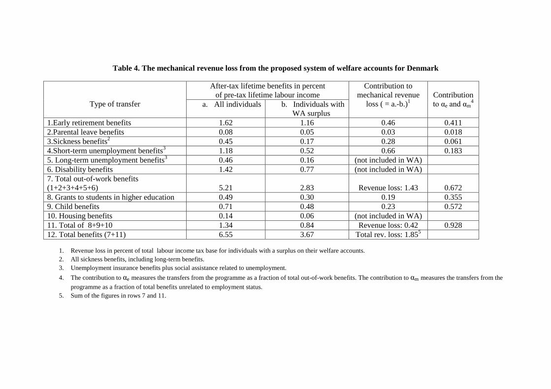
Table 4. The mechanical revenue loss from the proposed system of welfare accounts for Denmark

1. Revenue loss in percent of total labour income tax base for individuals with a surplus on their welfare accounts. 2. All sickness benefits, including long-term benefits. 3. Unemployment insurance benefits plus social assistance related to unemployment. 4. The contribution to αe measures the transfers from the programme as a fraction of total out-of-work benefits. The contribution to αm measures the transfers from the

programme as a fraction of total benefits unrelated to employment status. 5. Sum of the figures in rows 7 and 11.

Type of transfer

After-tax lifetime benefits in percent of pre-tax lifetime labour income

Contribution to mechanical revenue

loss ( = a.-b.)1

Contribution to αe and αm

4 a. All individuals b. Individuals with WA surplus

1.Early retirement benefits 1.62 1.16 0.46 0.411 2.Parental leave benefits 0.08 0.05 0.03 0.018 3.Sickness benefits2 0.45 0.17 0.28 0.061 4.Short-term unemployment benefits3 1.18 0.52 0.66 0.183 5. Long-term unemployment benefits3 0.46 0.16 (not included in WA) 6. Disability benefits 1.42 0.77 (not included in WA) 7. Total out-of-work benefits (1+2+3+4+5+6)

5.21

2.83

Revenue loss: 1.43

0.672

8. Grants to students in higher education 0.49 0.30 0.19 0.355 9. Child benefits 0.71 0.48 0.23 0.572 10. Housing benefits 0.14 0.06 (not included in WA) 11. Total of 8+9+10 1.34 0.84 Revenue loss: 0.42 0.928 12. Total benefits (7+11) 6.55 3.67 Total rev. loss: 1.855

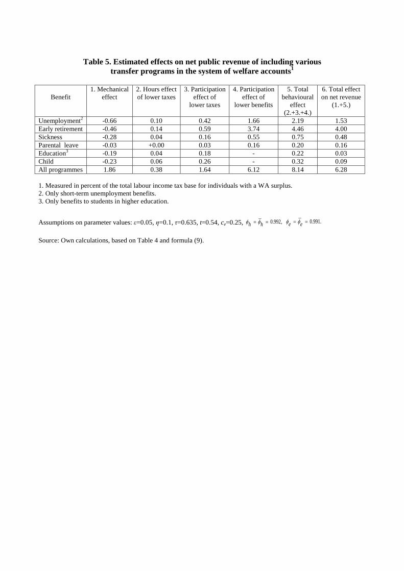
Table 5. Estimated effects on net public revenue of including various transfer programs in the system of welfare accounts1

Benefit 1. Mechanical

effect

2. Hours effect of lower taxes

3. Participation effect of

lower taxes

4. Participation effect of

lower benefits

5. Total behavioural

effect (2.+3.+4.)

6. Total effect on net revenue

(1.+5.)

Unemployment2 -0.66 0.10 0.42 1.66 2.19 1.53 Early retirement -0.46 0.14 0.59 3.74 4.46 4.00 Sickness -0.28 0.04 0.16 0.55 0.75 0.48 Parental leave -0.03 +0.00 0.03 0.16 0.20 0.16 Education3 -0.19 0.04 0.18 - 0.22 0.03 Child -0.23 0.06 0.26 - 0.32 0.09 All programmes 1.86 0.38 1.64 6.12 8.14 6.28 1. Measured in percent of the total labour income tax base for individuals with a WA surplus. 2. Only short-term unemployment benefits. 3. Only benefits to students in higher education.

Assumptions on parameter values: ε=0.05, η=0.1, τ=0.635, t=0.54, ce=0.25, 0.992,h hφ φ= = 0.991.e eφ φ= = Source: Own calculations, based on Table 4 and formula (9).

Table 6. The effects of the WA system on the public budget and on economic efficiency: sensitivity analysis1

Parameter

values Total efficiency

gain3

Total effect on net revenue4

Benchmark parameter values2

8.14

6.28

1h ea a= = 7.19 5.33 0.1ε = 8.52 6.67 0.05η = 4.26 2.41 0.15η = 12.02 10.16

1. All numbers are expressed in percent of the labour income tax base for individuals with a WA surplus. The scenario with the benchmark parameter values corresponds to the case considered in Table 5.

2. 0.05, 0.1, 0.635, 0.54, 0.25, 0.2.e h et c a aε η τ= = = = = = =

3. Revenue gain from behavioural responses, estimated from formula (9). 4. Estimated from formula (9).

Source: Own calculations, based on Table 4 and formula (9).