Efficient R Programming

Martin Morgan

Fred Hutchinson Cancer Research Center

30 July, 2010

Motivation

Challenges

I Long calculations: bootstrap, MCMC, . . . .

I Big data: genome-wide association studies, re-sequencing, . . . .

I Long × big: . . .

Solutions

I Avoid R programming pitfalls – very significant benefits.

I Parallel evaluation, especially ‘embarrassingly parallel’

I Large data management

Outline

Programming pitfallsPitfalls and solutionsMeasuring performanceCase Study: GWAS

Large data managementText, binary, and streaming I/OData bases and netCDF

Parallel evaluationEmbarrassingly parallel problemsPackages and evaluation modelsCase Study: GWAS (continued)

Resources

Programming pitfalls: easy solutions

I Input only required data

> colClasses <-

+ c("NULL", "integer", "numeric", "NULL")

> df <- read.table("myfile", colClasses=colClasses)

I Preallocate-and-fill, not copy-and-append

> result <- numeric(nrow(df))

> for (i in seq_len(nrow(df)))

+ result[[i]] <- some_calc(df[i,])

I Vectorized calculations, not iteration

> x <- runif(100000); x2 <- x^2

> m <- matrix(x2, nrow=1000); y <- rowSums(m)

I Avoid unnecessary character creation operations, e.g.,USE.NAMES=FALSE in sapply, use.names=FALSE in unlist.

Programming pitfalls: moderate solutions

I Use appropriate functions, often from specialized packages.

> library(limma) # microarray linear models

> fit <- lmFit(eSet, design)

I Identify appropriate algorithms, e.g., %in% is O(N), whereasnaive might be O(N2)

> x <- 1:100; s <- sample(x, 10)

> inS <- x %in% s

I Use C or Fortran code. Requires knowledge of otherprogramming languages, and how to integrate these into R

Measuring performance: timing

I Use system.time to measure total evaluation timeI gcFirst=TRUE for ‘garbage collection’

I Use replicate to average over invocations

> m <- matrix(runif(200000), 20000)

> replicate(5, system.time(apply(m, 1, sum))[[1]])

[1] 0.183 0.177 0.183 0.181 0.178

> replicate(5, system.time(rowSums(m))[[1]])

[1] 0.001 0.001 0.001 0.001 0.001

I Cautionary tale: http://tinyurl.com/29bd6xv

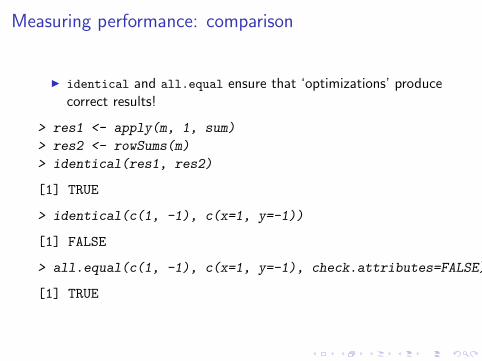
Measuring performance: comparison

I identical and all.equal ensure that ‘optimizations’ producecorrect results!

> res1 <- apply(m, 1, sum)

> res2 <- rowSums(m)

> identical(res1, res2)

[1] TRUE

> identical(c(1, -1), c(x=1, y=-1))

[1] FALSE

> all.equal(c(1, -1), c(x=1, y=-1), check.attributes=FALSE)

[1] TRUE

Measuring execution time: Rprof

> tmpf = tempfile()

> Rprof(tmpf)

> res1 <- apply(m, 1, sum)

> Rprof(NULL); summaryRprof(tmpf)

$by.selfself.time self.pct total.time total.pct

"apply" 0.16 80 0.20 100"FUN" 0.02 10 0.02 10"lapply" 0.02 10 0.02 10"unlist" 0.00 0 0.02 10

$by.totaltotal.time total.pct self.time self.pct

"apply" 0.20 100 0.16 80"FUN" 0.02 10 0.02 10"lapply" 0.02 10 0.02 10"unlist" 0.02 10 0.00 0

Measuring memory use: tracemem

I Enable memory profiling

> ~/src/R-devel/configure --help> ~/src/R-devel/configure --enable-memory-profiling> make -j

I Copy-on-change semantics

> x <- 1:10; tracemem(x)[1] "<0x1b1a8f8>"> y <- x # no change, so no copy> x[1] <- 2L # x, y now differ, so copytracemem[0x1b1a8f8 -> 0x1b1a8a0]:

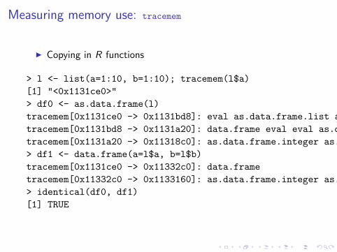
Measuring memory use: tracemem

I Copying in R functions

> l <- list(a=1:10, b=1:10); tracemem(l$a)[1] "<0x1131ce0>"> df0 <- as.data.frame(l)tracemem[0x1131ce0 -> 0x1131bd8]: eval as.data.frame.list as.data.frametracemem[0x1131bd8 -> 0x1131a20]: data.frame eval eval as.data.frame.list as.data.frametracemem[0x1131a20 -> 0x11318c0]: as.data.frame.integer as.data.frame data.frame eval eval as.data.frame.list as.data.frame> df1 <- data.frame(a=l$a, b=l$b)tracemem[0x1131ce0 -> 0x11332c0]: data.frametracemem[0x11332c0 -> 0x1133160]: as.data.frame.integer as.data.frame data.frame> identical(df0, df1)[1] TRUE

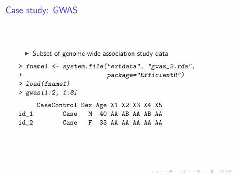
Case study: GWAS

I Subset of genome-wide association study data

> fname1 <- system.file("extdata", "gwas_2.rda",

+ package="EfficientR")

> load(fname1)

> gwas[1:2, 1:8]

CaseControl Sex Age X1 X2 X3 X4 X5id_1 Case M 40 AA AB AA AB AAid_2 Case F 33 AA AA AA AA AA

GWAS and glm

I Interested in fitting generalized linear model to each SNP

> snp0 <- function(i, gwas) {

+ snp <- gwas[[i+3L]]

+ glm(CaseControl ~ Age + Sex + snp,

+ family=binomial, data=gwas)$coef

+ }

> system.time(sapply(1:10, snp0, gwas))

user system elapsed1.700 0.102 1.919

GWAS case study: further directions

glm can be optimized for SNPs

I Build the design matrix for CaseControl ~ Age + Sex once,rather than once per SNP

I Use the estimate without the SNP as a starting point

I snpMatrix fits GLMs very efficiently

Outcome

I ∼ 1000 SNPs per second

Important lessons

I Careful optimization can often greatly reduce evaluation time

I Others may likely have done the work for you!

Outline

Programming pitfallsPitfalls and solutionsMeasuring performanceCase Study: GWAS

Large data managementText, binary, and streaming I/OData bases and netCDF

Parallel evaluationEmbarrassingly parallel problemsPackages and evaluation modelsCase Study: GWAS (continued)

Resources

Large data management

Putting appropriate data in memory

I An R analysis can make multiple copies of each data set

I Limits performance (I/O, but also calculations)

I Wastes system resources (e.g., decreasing the number ofparallel tasks that can be executed)

Solutions

I Text versus R binary files

I ‘Stream’ processing

I Data base use

I High-performance numeric storage

Text versus R binary files

I Text is slower than compressed binary

I Compressed binary is slower than binary

> ftmp <- tempfile()

> write.csv(gwas, ftmp)

> system.time(read.csv(ftmp, row.names=1))[[3]]

[1] 8.078

> save(gwas, file=ftmp)

> replicate(5, system.time(load(ftmp, new.env()))[[3]])

[1] 1.452 1.451 1.451 1.451 1.453

> save(gwas, file=ftmp, compress=FALSE)

> replicate(5, system.time(load(ftmp, new.env()))[[3]])

[1] 1.035 1.031 1.032 1.030 1.049

> unlink(ftmp)

‘Stream’ processing

I Read in a chunk, process, read in next chunk

I Use ‘connections’ to keep file open between chunks

I Good for very large data sets (if necessary)

I A few packages, e.g., biglm, exploit this model

I See readScript("fapply.R")

Data bases

SQL

I Represent data in a SQL data base

I Best for relational (structured) data of moderate (e.g.,millions of rows) size

I Not the best solution for, e.g., array-like numerical data

Use

I DBI package provides abstract interface

I RSQLite (built-in to R), RMySQL, RPostgreSQL, ... provideimplementations

Example: RSQLite set-up

> db0 <- tempfile()

> library(RSQLite)

> drv <- dbDriver("SQLite")

> conn <- dbConnect(drv, dbname=db0)

GWAS metadata

Create

> gwasPhenotypes <- gwas[,1:3]

> dbWriteTable(conn, "gwasPhenotypes", gwasPhenotypes)

[1] TRUE

Retrieve

> q <- dbSendQuery(conn, "SELECT * FROM gwasPhenotypes")

> fetch(q, n = 2) # first 2; n = -1 for all

row_names CaseControl Sex Age1 id_1 Case M 402 id_2 Case F 33

> invisible(dbClearResult(q)) # close out query

Clean-up

> invisible(dbDisconnect(conn))

NetCDF and the ncdf package

NetCDF and ncdf

I Network Common Data Form: array-oriented scientific dataI ncdf : R package for NetCDF access

I Warning: character arrays very inefficient in ncdf

I ncdf4 : recent; NetCDF 4 format; not yet avaiable forWindows

Data and library

> ngwas <- local({

+ x0 <- lapply(gwas[,-(1:3)], as.integer)

+ matrix(unlist(x0, use.names=FALSE), ncol=length(x0))

+ })

> ncdf0 <- tempfile()

> library(ncdf)

ncdf , continued

I Define dimensions and variable

> sampd <- dim.def.ncdf("Sample", "id", seq_len(nrow(ngwas)))

> snpd <- dim.def.ncdf("SNP", "id", seq_len(ncol(ngwas)))

> snpv <- var.def.ncdf("Genotype",

+ units="1: AA, 2: AB; 3: BB",

+ dim=list(sampd, snpd),

+ missval=-1L, prec="integer")

I Create file

> nc <- create.ncdf(ncdf0, snpv)

> put.var.ncdf(nc, snpv, ngwas)

> invisible(close(nc))

ncdf , continued

I Very favorable file I/O performance

> nc <- open.ncdf(ncdf0)

> system.time({

+ nc_gwas <- get.var.ncdf(nc, "Genotype")

+ })[[1]]

[1] 0.361

I Easy to obtains data slices

> g <- get.var.ncdf(nc, "Genotype", start=c(30, 100),

+ count=c(10, 20)) # samples 30:40, snps 100:120

> g <- get.var.ncdf(nc, "Genotype", start=c(1,1000),

+ count=c(-1, 100)) # all samples, snps 1000:1100

> invisible(close(nc))

Outline

Programming pitfallsPitfalls and solutionsMeasuring performanceCase Study: GWAS

Large data managementText, binary, and streaming I/OData bases and netCDF

Parallel evaluationEmbarrassingly parallel problemsPackages and evaluation modelsCase Study: GWAS (continued)

Resources

‘Embarrassingly parallel’ problems

Problems that are:

I Easily divisible into different, more-or-less identical,independent tasks

I Tasks distributed across distinct computational nodes.

I Examples: bootstrap; MCMC; row- or column-wise matrixoperations; ‘batch’ processing of multiple files, . . .

What to expect: ideal performance

I Execution time inversely proportional to number of availablenodes: 10× speed-up requires 10 nodes, 100× speeduprequires 100 nodes

I Communication (data transfer between nodes) is expensive

I ‘Coarse-grained’ tasks work best

Packages and other solutions

Package Hardware Challenges

multicore Computer Not Windows (doSMP soon)Rmpi Cluster Additional job management soft-

ware (e.g., slurm)snow Cluster Light-weight; convenient if MPI

not availableBLAS, pnmath Computer Customize R build; benefits math

routines onlyParallel interfaces

I Package-specific, e.g., mpi.parLapply

I foreach, iterators, doMC , . . . : common interface; faulttolerance; alternative programming model

General guidelines for parallel computing

I Maximize computation per job

I Distribute data implicitly, e.g., using shared file systemsI Nodes transform large data to small summary

I E.g.: ShortRead quality assessment.

I Construct self-contained functions that avoid global variables.

I Random numbers need special care!

multicore

I Shared memory, i.e., one computer with several cores

> system.time(lapply(1:10, snp0, gwas))user system elapsed1.672 0.016 1.687

> library(multicore)> system.time(mclapply(1:10, snp0, gwas))

user system elapsed1.864 0.348 1.119

multicore: under the hood

I Operating system fork: new process, initially identical tocurrent, OS-level copy-on-change.

I parallel: spawns new process, returns process id, startsexpression evaluation.

I collect: queries process id to retrieve result, terminatesprocess.

I mclapply: orchestrates parallel / collect

foreach

I foreach: establishes a for-like iterator

I %dopar%: infix binary function; left-hand-side: foreach;right-hand-side: expression for evaluation

I Variety of parallel back-ends, e.g., doMC for multicore;register with registerDoMC

> library(foreach)

> if ("windows" != .Platform$OS.type) {

+ library(doMC); registerDoMC()

+ res <- foreach(i=1:10) %dopar% snp0(i, gwas)

+ }

iterators and foreach

iterators package

I iter: create an iterator on an object

I nextElem: return the next element of the object

I Built-in (e.g, iapply, isplit) and customizable

> snp1 <- function(snp, gwas) {

+ glm(CaseControl ~ Age + Sex + snp,

+ family=binomial, data=gwas)$coef

+ }

> snps <- gwas[,11:20]

> res <- foreach(it=iter(snps, "column")) %dopar%

+ snp1(it, gwas)

Rmpi on a cluster

I ‘Message passing’ interface (MPI)

Players

I slurm: allocate resources, e.g., salloc -N 4 allocates 4nodes for computation

I mpi: e.g., mpirun -n 1 starts a program on one node

I R and the Rmpi package

Interactive Rmpi : manager / worker

hyrax1:~> salloc -N 4 mpirun -n 1 R --interactive --quietsalloc: Granted job allocation 239631> library(Rmpi)> mpi.spawn.Rslaves()[...SNIP...]> mpi.parSapply(1:10,

function(i) c(i=i, rank=mpi.comm.rank()))[,1] [,2] [,3] [,4] [,5] [,6] [,7] [,8] [,9] [,10]

i 1 2 3 4 5 6 7 8 9 10rank 1 1 1 2 2 3 3 4 4 4> mpi.quit()salloc: Relinquishing job allocation 239631

Manager / worker

I ‘Manager’ script that spawns workers, tells workers what todo, collates results

I Submit as ‘batch’ job on a single R node

I View example script with readScript("spawn.R")

hyrax1:~> salloc -N 4 mpirun -n 1 \R CMD BATCH /path/to/spawn.R

Single instruction, multiple data (SIMD)

I Single script, evaluated on each node, readScript("simd.R").

I Script specializes data for specific node

I After evaluation, script specializes so that one node collatesresults from others

hyrax1:~> salloc -N 4 mpirun -n 4 \R CMD BATCH --slave /path/to/simd.R

Case study: GWAS (continued)

I Readily parallelized – glm for each SNP fit independently

I Divide SNPs into equal sized groups, one group per node

I SIMD evaluation model

I Need to manage data – appropriate SNPs and metadata toeach node

Important lessons

I Parallel evaluation for real problems can be difficult

I Parallelization after optimization

I Optimize / parallelize only after confirming that no one elsehas already done the work!

Case study: GWAS (concluded)

Overall solution

I Optimize glm for SNPs

I Store SNP data as netCDF, metadata as SQL

I Use SIMD model to parallelize calculations

Outcome

I Initially: < 10 SNPs per second

I Optimized: ∼ 1000 SNP per second

I 100 node cluster: ∼ 100, 000 SNP per second

Outline

Programming pitfallsPitfalls and solutionsMeasuring performanceCase Study: GWAS

Large data managementText, binary, and streaming I/OData bases and netCDF

Parallel evaluationEmbarrassingly parallel problemsPackages and evaluation modelsCase Study: GWAS (continued)

Resources

Resources

I News group:https://stat.ethz.cb/mailman/listinfo/r-sig-hpc

I CRAN Task View: http://cran.fhcrc.org/web/views/HighPerformanceComputing.html

I Key packages: multicore, Rmpi , snow , foreach (and friends);RSQLite, ncdf