efficient quarantining of scanning worms optimal detection and coordination
TRANSCRIPT
7/30/2019 Efficient Quarantining of Scanning Worms Optimal Detection and Coordination
http://slidepdf.com/reader/full/efficient-quarantining-of-scanning-worms-optimal-detection-and-coordination 1/13
Efficient quarantining of scanning worms:
optimal detection and coordinationA. Ganesh, D. Gunawardena, P. Key, L. Massoulié
Microsoft Research, Cambridge, U.K.
Email: ajg,dinang,peter.key,[email protected]
J. ScottEE & CS Department, UC Berkeley
Abstract— Current generation worms have causedconsiderable damage, despite their use of unsophis-ticated scanning strategies for detecting vulnerablehosts. A number of adaptive techniques have beenproposed for quarantining hosts whose behaviour
is deemed suspicious. Such techniques have beenproven to be effective against fast scanning worms.However, worms could evade detection by being lessaggressive. In this paper we consider the interplaybetween worm strategies and detection techniques,which can be described in game-theoretic terms.
We use epidemiological modelling to characterisethe outcome of the game (the pay-off function), asa function of the strategies of the worm and thedetector. We design detection rules that are optimalagainst scanning worms with known characteristics.We then identify specific detection rules that areclose to optimal, in some mathematically precisesense, against any scanning worm. Finally, we designmethods for coordinating information among a set
of end-hosts, using Bayesian decision theory. Weevaluate the proposed rules using simulations drivenby traces from a corporate environment of 600 hosts,and assess the benefits of coordination.
I. INTRODUCTION
A worm is a self-propagating malicious pro-
gram that exploits security vulnerabilities and does
not require user action to propagate. Weaver et
al [16] give a general taxonomy of worms. They
list target discovery – the mechanism by which a
worm discovers vulnerable hosts – as one of the
critical factors of a worm’s strategy. Current gener-
ation worms have typically used simple strategies,
such as random or sequential scanning of the
address space, to discover vulnerable hosts. With
the address space the IPv4 namespace, the Code
Red worm [11] managed to infect some 360,000
hosts in 24 hours, Blaster infected around 150,000
hosts in days while Slammer [10] infected 75,000
hosts in less than 15 minutes.
Several techniques to detect and contain worms
have been proposed and implemented. Many of
these combine some form of anomaly detection
with either rate-limiting or quarantining the host.
A simple example is Williamson’s throttle [17],[15], which combines a rate throttle with an LRU
whitelist cache to limit the rate of connections to
new hosts to 1Hz. Such rate-limit throttles can
cause problems for high-load machines such as
servers, or for peer-to-peer applications. Schechter
et al. [13] use a credit throttle combined with
a reverse sequential hypothesis test that looks
at both failures and successes. A similar idea
was proposed to deal with port-scanning in gen-
eral [6]. Anomaly detection schemes have the
advantage that they are exploit-neutral, and so
they work for zero-day worms (worms targeting an
unknown vulnerability). They can be implementedby subnet-level intrusion detectors [13] or as part
of network level intrusion detectors at gateways, or
on the end-hosts themselves. Honey-pots and pop-
ulating the address space with dark addresses are
other ways to detect malicious scanning attempts.
Detecting anomalous behavior is just one line
of defence. Another technique is packet payload
monitoring, used for example in Autograph [7];
by detecting a worm signature, worm packets can
be filtered out at network routers. This relies on
detection, identification and probably infection, so
has some difficulties with zero-day exploits, as
well as with polymorphic worms. A promising
alternative approach based on using a collaborative
system for broadcasting self-certifying alerts [4]
has also been proposed recently. Ideally security
vulnerabilities are themselves prevented, an area
the programming language community is address-
ing. But while vulnerabilities do exist, we would

7/30/2019 Efficient Quarantining of Scanning Worms Optimal Detection and Coordination
http://slidepdf.com/reader/full/efficient-quarantining-of-scanning-worms-optimal-detection-and-coordination 2/13
like to detect worms and stop their spread. Despite
the different approaches described above, we be-
lieve that detecting anomalous scanning behaviour
continues to be a useful weapon against worms,
and that in practice multi-faceted defence has
advantages.
More sophisticated scanning strategies involve
harvesting known addresses, e.g., by using address
information on the local host (such as IP or layer
2 information available through local host files,
netstat statistics, arp tables etc, or addresses in
local address books). Such ‘topological’ worms
are extremely difficult to detect since malicious
behavior may be hard to distinguish from normal
behavior, and are outside the scope of this paper.
Our focus in this paper is on detecting anoma-
lies due to worm scanning behaviour, basedon end-system monitoring and co-ordinated re-
sponses. In section II we give an analytic treatment
of countermeasures based on epidemic models and
use this to analyse particular throttling schemes.
In section III we look at optimal detection mech-
anisms, based on the CUSUM technique which
is well-known in the control theory literature.
These detection mechanisms have close links to
the reverse sequential likelihood ratio test of [6],
[13], though we specifically focus on failures to
avoid a worm gaming the mechanism. We view
the interaction between the worm and detector
as a game; the detector chooses a strategy forquarantining, the worm chooses a scanning rate
and the pay-off is the speed of spread (the growth
exponent of the epidemic). This enables us to
determine the Minimax solution, i.e. the best de-
tector against the worst worm. We further derive
suboptimal practical policies. In section V, we
describe how to coordinate information amongst a
set of hosts by using a Bayesian decision theoretic
framework, in order to improve the detection of
misbehaving hosts. Note that this is different from
an aggregate detector: we are pooling individual
information and then feeding that information
back to identify the affected hosts, something an
aggregate detector cannot do unless it sees all the
information available to individual hosts. We use
trace-driven simulations to assess the performance
of worms and countermeasures, with and without
coordination. For our data we find that without
coordination the optimal (slow-scanning) worm
can still infect a significant fraction of the network,
whereas co-ordination can further limit the spread.
II. EPIDEMIOLOGICAL MODELLING OF
COUNTERMEASURES
The aim of this section is to describe the
outcome of a worm infection in a network with
countermeasures deployed at every host. We focus
on two types of countermeasures: (a) throttling
schemes, whereby the rate at which a host can
make new connections is reduced, and (b) quar-
antining schemes, whereby a host, when deemed
infected, is denied further access to other hosts.
Conveniently, the effect of both types of counter-
measures can be envisaged in a single framework,
which we now describe.
A. General framework
Consider an address space of size Ω populated
by N hosts sharing some vulnerability which is
exploited by the worm. When host j becomes
infected, it scans the address space at rate vjand infects any vulnerable host it locates. We
use the following notation for key parameters
throughout this section: α = N/Ω is the fraction
of the scanned address space which is populated
by addresses corresponding to vulnerable hosts; vis the scanning rate of infected hosts; r(t) is the
fraction of vulnerable hosts that has been infected
by time t. Formally, we consider a sequence of such systems indexed by N , and assume that
α and v remain constant. Suppose first that no
countermeasures are in place. If we assume that
the scan times are described by a Poisson process,
then r(t) evolves as a Markov process. As N tends to infinity, the sequence of Markov process
describing the fraction of infected hosts converges
to the solution of a differential equation. This
follows by a straightforward application of Kurtz’s
theorem [14, Theorem 5.3]. For background on
differential equation models of epidemics, see
[5]; for applications to Internet worms, see [18]
and references therein. We shall use differential
equations to model the evolution of r over time,
including the impact of countermeasures. While
we omit proofs, it should be understood that
these models arise in the large population limit
described formally above, and that their use can
be rigorously justified using Kurtz’s theorem.

7/30/2019 Efficient Quarantining of Scanning Worms Optimal Detection and Coordination
http://slidepdf.com/reader/full/efficient-quarantining-of-scanning-worms-optimal-detection-and-coordination 3/13
In addition to the above parameters, we shall
summarize the effect of the countermeasure by a
reduction factor, θ(t), which affects the scanning
rate of a host which has been infected for t time
units. More precisely, we assume such a host
scans the total address space on average at a rate
of vθ(t) connection attempts per second. Under
these assumptions, we can show that the infected
fraction r(t) evolves according to the differential
equation:
dr
dt= αv(1−r(t))
r(0)θ(t) +
t0
r(s)θ(t − s)ds
.
Indeed, the number of hosts infected in some small
time interval [s, s + ds] is r(s)ds. At time t >s, these scan on average at a rate of vθ(t − s).
Such scans are targeted at vulnerable addresses
with probability α; the targets have not yet beeninfected with probability 1 − r(t). Summing over
all such intervals [s, s + ds], and accounting for
infections due to initially infected hosts, yields this
equation.
We are interested only in the behaviour of
epidemics until r(t) reaches some small δ , which
we take to reflect global epidemic outbreak; think
of δ being 5% for instance. We may thus consider
the tight upper bound to r(t), which solves the
linear equation obtained by suppressing the factor
(1 − r(t)) in the above. This now reads
r(t) = vα
r(0)θ(t) + t0
r(s)θ(t − s)ds
.
Upon integrating, this reads
r(t) = r(0) +
t0
r(t − s)vαθ(s)ds. (1)
This is a classical equation, known as a renewal
equation; see e.g. [1], Chapter V1. The epidemics
will spread or die out exponentially fast depending
on whether the integral ∞0
vαθ(s)ds is larger or
smaller than one. This integral yields the mean
number of hosts infected by a single initial infec-
tive, which is referred to as the basic reproduction
number in epidemiology. In the critical case wherethis integral equals one, for large T , we have by
the renewal theorem the estimate
r(T ) ∼r(0)T
vα ∞0
sθ(s)ds· (2)
1This derivation is similar to that of Lotka’s integral equationof population dynamics; see [1], p.143.
In the subritical case (i.e. when vα ∞0
θ(s)ds <1), then for large T one has that
r(T ) ∼r(0)
1 − vα ∞0 θ(s)ds
· (3)
In the supercritical case when vα ∞0 θ(s)ds > 1,
let ν > 0 be such that
vα
∞0
e−νsθ(s)ds = 1. (4)
Then one has the estimate for large T :
r(T ) ∼ eνT r(0)
vα ∞0
se−νsθ(s)ds· (5)
The parameter ν is called the exponent of the
epidemics; it determines the doubling time of the
epidemics, which reads ν −1 ln(2).
These general results indicate that, in orderfor the epidemics to remain controlled in a time
interval of length T the epidemics have to be either
subcritical, or supercritical with a doubling time of
the order of T . Indeed, in the supercritical case,
r(T ) may still be small provided νT is small.
In the present context, a design objective for
countermeasures is to prevent global spread before
a vulnerability is identified, patches are devel-
opped and distributed. We may then take T to be
of the order of days.
It should be noted that the above framework can
be extended to consider more general scanning
rate profiles, e.g. captured by a scanning speed
v(t) depending on the time t since infection. All of
the above discussion carries over to this case if we
introduce the function S (t) of scanning attempts
that can be made within t time units following in-
fection, which summarizes the interaction between
the worm and countermeasure, and if we replace in
the above equations vθ(t) by the derivative S (t).
We now apply this general framework to spe-
cific scenarios, by identifying the function θ(t)corresponding to specific countermeasures.
B. Quarantining mechanisms
We first consider the case of quarantining mech-
anisms, in which a host’s connection attempts
are unaffected until some random time when it
is completely blocked. Let τ denote the random
time it takes after infection for quarantining to
take place. Then the rate at which a host which
has been infected for t seconds issues scans is

7/30/2019 Efficient Quarantining of Scanning Worms Optimal Detection and Coordination
http://slidepdf.com/reader/full/efficient-quarantining-of-scanning-worms-optimal-detection-and-coordination 4/13
given by vP(τ ≥ t), where P(τ ≥ t) denotes the
probability that the random detection time is larger
than or equal to t. This corresponds to setting
θ(t) = P(τ ≥ t). As ∞0
θ(t)dt equals the aver-
age detection time, denoted τ , the general results
described above imply that the epidemic will be
subcritical, critical or supercritical as αvτ is less
than, equal to or greater than one respectively.
C. Throttling mechanisms
We now consider mechanisms where, which
reduce the rate at which a host can make new
connections when it is deemed suspicious. This
is expected to effectively shut down the host if
scanning is at a high rate. In the case of low
scanning rate, this could provide benefits without
incurring the penalty of shutting down the host.
a) Williamson’s throttle: Consider
Williamson’s throttle, as proposed in [17].
According to this scheme, a host’s connection
requests go through a FIFO queue, and are
processed at rate c connections per second.
Assuming the host generates w non-wormy
connection attempts per second, we find that the
worm effectively scans at a rate of vc/(v +w) if it
competes fairly with the host’s legitimate traffic,
and if the submitted rate v + w is larger than c.
The slow-down factor is then θ(t) = c/(v + w),
as long as the host is not blocked.
Assume now, as in Williamson’s proposal, thatthe host is quarantined when the queue reaches
some critical level q . The time it takes to reach that
level is τ fill = q/(v+w−c). We thus have θ(t) =c/(v+w) if t ≤ τ fill, and θ(t) = 0 otherwise. The
quantity characterising criticality of the epidemics
then reads
αv
∞0
θ(t)dt = αvc
v + wτ fill.
In the supercritical case, Equation (4) again char-
acterises the epidemics’ exponent.
b) Max-Failure throttle: The Max-Failure
(MF) scheme that we now propose is meant to
throttle connection attempts to ensure that the
long-run rate of failed connection attempts is be-
low some pre-specified target rate, λf . It is similar
in spirit to the Leaky Bucket traffic scheduler (see
e.g. [8], [3] and references therein), and enjoys
similar optimality properties. It works as follows.
Connection attempts are fed to a queue, and need
to consume a token to be processed. There is
a token pool, with maximal size B; the pool is
continuously replenished at a rate λf . Finally,
when a previously made connection attempt is
acknowledged, the token it has used is released
and put back in the pool 2. The appeal of MF is
captured by the following proposition.
Proposition 1: Provided that successful con-
nection attempts always get acknowledged less
than 1/λf seconds after the connection request
has been sent, under MF, in any interval [s, t],
the number of connection attempts that resulted
in failure is at most B + λf (t − s).
Furthermore, MF schedules connection requests
at the earliest, among all schedulers that satisfy
this constraint on the number of failed connection
attempts in each interval [s, t], and that do not haveprior information on whether connection attempts
will fail or not.
Proof: The first part is easily established,
and we omit the detailed argument due to lack
of space. For the second part, consider a process
of connection requests, and an alternative scheme
that would at some time t schedule a request that
is backlogged at t under MF. Thus the MF token
pool contains less than one unit at t. Equivalently,
there exists some s < t such that under MF, the
number n of attempted and not yet acknowledged
connection attempts made in interval [s, t] verifies
n + 1 > B + (t − s)λf . If these connectionattempts, as well as the additional one made by
the alternative throttle, all fail, then this throttle
will experience at least n + 1 > B + (t − s)λf
failures within interval [s, t], which establishes the
claim.
Consider now hosts who submit non-wormy
connection requests at a rate w, a proportion pf of
which fail. Assume as before that a worm submits
scan attempts at a rate of v, a proportion (1− α)of which are directed at non-vulnerable hosts.
We make the additional assumption that scanning
attempts result in failures when targeted at non-
vulnerable hosts, so that for an infected host, the
rate of failed connection attempts due to worm
scanning is v(1 − α).
2Schechter et al. [13] have proposed a similar scheme, whichdiffers in that they replace two instead of one token into thepool upon acknowledgement.

7/30/2019 Efficient Quarantining of Scanning Worms Optimal Detection and Coordination
http://slidepdf.com/reader/full/efficient-quarantining-of-scanning-worms-optimal-detection-and-coordination 5/13
Assuming that the failure rate in the absence of
throttling, namely pf w + (1−α)v, is greater than
λf , then after infection the token pool is emptied
in time τ empty = B/( pf w+(1−α)v), after which
connection attempts are slowed down by a factor
of λf /( pf w+(1−α)v). Thus, for the MF throttle,
we have the characterization
θ(t) =
1 if t ≤ τ empty,
λf pf w+(1−α)v
otherwise.(6)
Assuming further that, as in Williamson’s throttle,
the host gets blocked once there are q backlogged
requests, we find that it takes
τ fill =q
(v + w)(1 − λf /( pf w + (1 − α)v))]
seconds to quarantine the host once its token poolis exhausted. The quantity characterising critical-
ity of the epidemics then reads
αvB
pf w + (1 − α)v+
λf q (v + w)−1
pf w + (1 − α)v − λf ·
The growth exponent can be calculated as before
from Equation (4) in the super-critical case.
III. OPTIMAL DETECTION PROCEDURES
The aim of this section is to describe optimal
tests for detecting infections under specific as-
sumptions on the probabilistic model of a host’s
normal behaviour and worm behaviour. We con-sider detection procedures based on the observa-
tion of failed connection attempts only, beacuse
it is straightforward for a worm to artificially
increase the number of successful connections,
and thus defeat detectors based on the ratio of
failures to successes.
The model we take of normal behaviour is the
following. A host attempts connections that fail at
a rate λ0, with the failure times being the points
of a Poisson process. This assumption is made for
the sake of tractability. It is however plausible if
failures are rare, since Poisson processes are good
approximations for processes of rare, independent
instances of events.
If the host is infected, the worm scans occur
at the points of an independent Poisson process
of rate v. Again, this assumption is made for the
sake of tractability. The worm scans are successful
with probability α and the successes form an iid
Bernoulli sequence. This is consistent with the as-
sumption of a randomly scanning worm that picks
target addresses uniformly at random from the
whole address space. Hence, the aggregate failure
process is Poisson with rate λ1 = λ0 + (1 − α)v.
We first assume that λ0 and λ1 are known, in
order to get bounds on the best case achievable
performance. We shall also discuss schemes that
are close to optimal and do not rely on knowledge
of these parameters in the next subsection.
A. Optimal CUSUM test for known scan rates
The objective is to detect that a host is infected
in the shortest possible time after infection, while
ensuring that the false alarm rate is acceptably
low. This is a changepoint detection problem andit is known that the CUSUM strategy described
below has certain desirable optimality properties
(see, e.g., [9], [12]).
Note that this strategy is very similar to
the detection mechanism proposed in [13].
Given a sequence of observed inter-failure times
t1, t2, t3, . . ., we declare that the host is infected
after the R-th failure time, where
R = inf
n : max1≤k≤n
n
i=klog
f 1(ti)
f 0(ti)
≥ c
. (7)
Here, c is a specified threshold, and f 0 and f 1are densities under the null hypothesis that the
machine isn’t infected and the alternative hypoth-
esis that it is, i.e., f i(t) = λie−λit for t ≥ 0 and
i = 0, 1.
In words, we declare the machine to be infected
when the log likelihood ratio of its being infected
to its being uninfected over some finite interval
in the past exceeds a threshold, c. In order to
implement the test, we do not need to maintain
the entire history of observations and compute the
maximum over k ≤ n as above. The same quantity
can be computed recursively as follows. Define
Q0 = 0, and for i ≥ 1,
Qi = max
0, Qi−1 + logf 1(ti)
f 0(ti)
. (8)
The above recursion is known as Lindley’s equa-

7/30/2019 Efficient Quarantining of Scanning Worms Optimal Detection and Coordination
http://slidepdf.com/reader/full/efficient-quarantining-of-scanning-worms-optimal-detection-and-coordination 6/13
tion and its solution is
Qn = max
0, max
1≤k≤nn
i=k logf 1(ti)
f 0(ti)
= max0≤k≤n
(n − k)log
λ1λ0
− (λ1−λ0)(T n−T k)
(9)
where T n =n
i=1 ti is the time of the nth
failure. Now, by (7), R = inf n : Qn ≥ c.
In the literature on change point detection prob-
lems, the random variable R is called the run
length. The results in [9] imply that the CUSUM
test is optimal in that it minimizes the expected
time between infection and detection, given a tar-
get false positive rate, characterised by the average
run length E [R] when the host is uninfected. We
now obtain an estimate of this quantity.
Observe that the process Qi is a random walk
reflected at 0; under the null hypothesis that
the machine is uninfected, the free random walk
(without reflection) has negative drift. We want to
compute the level-crossing time for this random
walk to exceed a level c. Using standard large
deviation estimates for reflected random walks, it
can be shown that, for large c,
1
clog E 0[R] ∼ θ∗ := supθ > 0 : M (θ) ≤ 1,
(10)
where
M (θ) = E 0
exp
θ log f 1(ti)f 0(ti)
.
Here, we use the subscript 0 to denote that ex-
pectations are taken with respect to the distribu-
tion of ti under the null hypothesis, i.e., ti are
i.i.d., exponentially distributed with mean 1/λ0.
A straightforward calculation yields
M (θ) =
λ0
λ0+θ(λ1−λ0)
λ1λ0
θif θ > − λ0
λ1−λ0
+∞ otherwise.
From this, it can be readily verified that θ∗ = 1 .
We may wish to choose the threshold c so thatthe false alarm probability within some specified
time interval T , say one month or one year,
is smaller than a specified quantity . This is
equivalent to requiring that P (R ≤ λ0T ) < .
Using the so-called Kingman bound (see e.g. [2])
P (Qi ≥ c) ≤ e−θ∗c with θ∗ = 1,
and the union bound
P (R ≤ λ0T ) ≤λ0T
i=1 P (Qi ≥ c) ≤ λ0T e−θ∗c,
we find that the constraint P (R ≤ λ0T ) < is
satisfied provided
c ≥ logλ0T
. (11)
B. Subptimal detectors for unknown scan rates
In this section, we ask the following question:
given a bound ν on the acceptable growth rate of
the epidemic, is it possible to design a detector
that restricts the growth rate to no more than
ν , while simultaneously ensuring that the false
alarm probability over a specified time window
T doesn’t exceed a specified threshold ? Theanswer would define a feasible region that imposes
fundamental limits on detector performance.
In the most general setting, we would allow for
all possible worm scanning profiles, but we restrict
the strategy space by considering only constant
scanning rates. Thus, the worm can choose an
arbitrary scanning rate z; then, for each t, it makes
zt scanning attempts in the first t time units after
infecting a host. Of these, (1 − α)zt are failures
on average.
To start with, we consider general detector pro-
files. We shall then show that the optimal detector
is well approximated by a CUSUM detector. Now,an arbitrary detector can be specified by a function
F (·) which determines the maximum number of
failed connection attempts possible in any contigu-
ous time window before the host is quarantined.
Given F (·) and z, the maximum scanning rate
possible at time t is given by
θ(t) =
z, t ≤ tz,0, t > tz,
where tz ≥ 0 solves F (tz) = ( 1 − α)ztz;
take tz = ∞ if this equation has no solution.
Substituting this in (4), we find that the growth
exponent is bounded above by ν provided the
following inequality is satisfied:
α
tz0
ze−νtdt ≤ 1, i.e., 1 − e−νtz ≤ν
αz.
We want this inequality to hold for every z. Now,
each choice of z yields a tz as noted above. Hence,

7/30/2019 Efficient Quarantining of Scanning Worms Optimal Detection and Coordination
http://slidepdf.com/reader/full/efficient-quarantining-of-scanning-worms-optimal-detection-and-coordination 7/13
expressing z in terms of F (·) and tz , we can
rewrite the above inequality as
1 − e−νt ≤(1 − α)νt
αF (t)(12)
or equivalently,
F (t) ≤1 − α
α
νt
1 − e−νt, (13)
for all positive t. The above inequality yields a
necessary and sufficient condition for a detector
to guarantee the bound ν on the worm growth
exponent, for arbitrary choice of worm scanning
rate z. In other words, defining F (·) with equality
above yields the optimal detector in the following
sense: any detector which guarantees a worm
growth exponent no bigger than ν against constant
rate worms with arbitrary scanning rate will haveat least as large a false alarm rate.
The optimal detector has the property that the
worm growth exponent is insensitive to the scan-
ning rate (so long as the scanning rate is large
enough that it will eventually result in quarantine).
Thus, no cleverness is required on the part of the
worm designer if the optimal detector is employed.
Note that we are implicitly considering a game
between detectors and worms, where the worm
has second mover advantage. This is a realistic
assumption in a scenario where there is a large
installed base of worm detection software, and
worm designers could use their knowledge of this
software in specifying worm parameters.
Now, we could compute the false alarm rate for
the optimal detector as defined above. However,
in practice, it is not straightforward to enforce an
envelope with arbitrary shapes as above, whereas
we saw that an affine envelope corresponds simply
to a queue. Therefore, we first find an affine
function that is a lower bound to the RHS of (13).
It is readily verified that
F (t) =1 − α
α 1 +νt
2 (14)
is such a lower bound. In particular, using F (·)specified by (14) guarantees that the worm growth
rate is smaller than ν , since F (·) imposes a
more stringent bound on the number of failed
connections than the optimal detector.
Combining the specific choice for F given in
(14) together with the condition for achieving
target false alarm probabilities of every T time
units given in (11), we arrive at the following:
Proposition 2: Let λ0 be the rate at which hosts
fail due to non-wormy traffic, and let α be a known
bound on the fraction of address space occupied
by vulnerable hosts. Let be the target probability
of false alarms over a time horizon of T . Then one
can tune the parameters of CUSUM detectors so
that the exponent of the epidemics is not larger
than
ν max = 2λ01 − 2α
(1 − α)c
exp
αc
1 − 2α
− 1
(15)
for any worm that scans at constant rate. The
CUSUM detector satisfying these properties is
characterized by the choice of c as in Equa-
tion (11), and the following choice of λ1:
λ1 = λ0 exp
αc
1 − 2α
· (16)
Conversely, for any detector guaranteeing that
no constant scanning rate can achieve a growth
exponent bigger than ν max/2, the false alarm
probability over time horizon T is at least .
Remark 1: Note the slackness between the first
statement and its converse: by restricting to
CUSUM detectors, we are losing at most a factor
of two in the maximal achievable growth expo-
nent.
Proof: Observe from (7) and (9) that themaximum number of failed connection attempts
allowed by a CUSUM detector up to time t,
denoted n(t), must satisfy
[n(t) − 1]logλ1λ0
− (λ1 − λ0)t ≤ c. (17)
This also reads
n(t) ≤ 1 +c
log(λ1/λ0)+
λ1 − λ0log(λ1/λ0)
t.
Thus, if we identify the coefficients in this affine
constraint with those of the function F in (14), by
the preceding discussion it is guaranteed that no
constant scanning worm with success rate below
α can achieve an exponent bigger than ν . This
identification of coefficients yields1−αα = 1 + c
log(λ1/λ0),
1−αα
ν 2 = λ1−λ0
log(λ1/λ0)·

7/30/2019 Efficient Quarantining of Scanning Worms Optimal Detection and Coordination
http://slidepdf.com/reader/full/efficient-quarantining-of-scanning-worms-optimal-detection-and-coordination 8/13
The first relation is equivalent to (16), while the
second one gives the value of ν as in (15).
Conversely, note that the affine function F (t)as in (14) is larger than the function
G(t) :=1 − α
α
(ν/2)t
1 − e−(ν/2)t,
that is the right-hand side of Equation (13) with
ν replaced by ν/2. Hence, the affine constraint is
weaker than the optimal detector for ensuring the
bound ν/2 on the growth rate, and thus incurs a
lower false positive rate.
IV. EXPERIMENTS
We now describe experiments exploiting a traf-
fic trace, which was collected over 9 days at
a corporate research facility comprising of the
order of 500 workstations and servers. The IPand TCP headers were captured for all traffic
crossing VLANs on the on-site network (i.e. be-
tween machines on-site). The traffic capture (using
the NetMon2 tool) was post-processed to extract
TCP connection attempts. We consider only TCP
connections internal to the corporate environment
in what follows. Hence the experiments to be
described reflect the ability of worm detectors to
contain the spread of worms inside a corporate
environment.
Figure 1 represents the cumulative distribution
functions of the number of destinations to which
sources experience failed connection attempts.There is one curve per day of the trace. We
observe that 95% of sources fail to less than 20
destinations each day, and all sources fail to less
than 45 distinct destinations each day. The median
number of distinct addresses to which sources fail
is between 2 and 5 per day.
In a practical implementation of the CUSUM
detector, we would maintain a white list of re-
cently used addresses, as in the previous proposals
[17], [13]. Connection attempts to addresses in
the white list bypass the detector. Thus, repeated
failures to the same address would be counted as
one failure at the detector. Under such a scheme,
failures seen by the detector are expected to be
rare, and uncorrelated. This provides justification
for the assumption that failures follow a Poisson
process.
Figure 2 shows the cumulative distribution func-
tion per source of the total number of failed
0 5 10 15 20 25 30 35 40 450
0.1
0.2
0.3
0.4
0.5
0.6
0.7
0.8
0.9
1
x
F ( x )
cdf’s of number of destinations to which there are failures, per source
day1
day2
day3
day4
day5
day6
day7day8
day9
Fig. 1. Cumulative distribution function of numbers of destinations to which sources fail, from corporate trace.
connection attempts that would be measured by
a CUSUM detector over the whole 9-day trace
duration.
0 50 100 150 2000
0.1
0.2
0.3
0.4
0.5
0.6
0.7
0.8
0.9
1
x
F ( x )
Empirical CDF of number of failures per source, local caches 5−fail 5−success
Fig. 2. Cumulative distribution function of numbers of failuresper source, using white lists, over 9 days.
This figure is produced with a combined white
list mechanism, comprising the last five addresses
to which there have been failed connection at-
tempts, and the last five addresses to which there
have been successful connection attempts. These
are easily maintained by using the LRU (Least
Recently Used) replacement strategy. W e observe
that over 9 days, 95% of sources would have less
than 50 failures to addresses not in the cache,
while no source ever experiences more than 200
failures. This suggests that we chose background

7/30/2019 Efficient Quarantining of Scanning Worms Optimal Detection and Coordination
http://slidepdf.com/reader/full/efficient-quarantining-of-scanning-worms-optimal-detection-and-coordination 9/13
failure rate λ0 of the order of one failure per hour 3.
We now assess how CUSUM detectors would
perform in such a corporate environment. Specifi-
cally, we fix a target false positive probability =e−1 per year4. We then use the CUSUM detector
described in Proposition 2, which we know will
guarantee a bound on the growth exponent not
larger than twice the best possible bound, given
the false positive constraint. We then evaluate
the largest possible growth rate for this CUSUM
detector from Equation (15). Figure 3 plots the
corresponding time for the worm to grow ten-fold,
that is log(10)/ν max versus the bound α on the
fraction of vulnerable hosts.
We see that ten-fold increase will take of the
order of more than a day provided α is less
than 0.04. Thus, in networks with at most thisfraction of vulnerable hosts, this kind of detectors
will slow down epidemics sufficiently for human
intervention, e.g. development and distribution of
patches, to take over.
Recently, automatic patch generation and dis-
tribution schemes have been proposed (see [4])
which may have reaction times of the order of
tens of seconds. As we see from Figure 3, when
α is as large as 0.25, our detectors can force the
time to a ten-fold increase to be larger than six
minutes, which is well within the scope of such
schemes.
To complement these analytical evaluations, wehave run trace-driven simulations, with one ini-
tially infected host scanning randomly, and suc-
cessfully finding a victim 25% of the time, and
where each host runs the CUSUM detector tuned
as in Proposition 2, with a failure rate λ0 of once
per hour, and a target false positive rate as above.
Figure 4 illustrates the cumulative distribution
function of the number of hosts eventually in-
fected after 30 minutes, for various worm scanning
speeds. Each curve is obtained from 40 simulation
runs. We observe that with the slower scanning
speed of 0.01 attempts a second, the spread is
consistently larger than with the higher scanningspeeds of 0.1 and 1 attempts per second. With a
3Clearly, λ0 may be different in other, non-corporate envi-ronments; for example, there were no P2P applications in thetrace we studied.
4As the time to a false alarm is roughly exponentiallydistributed, this choice is consistent with an average of onefalse alarm per year.
0 0.05 0.1 0.15 0.2 0.2510
−1
100
101
102
103
104
Worm growth rate with CUSUM detector
Success probability α
T I m e t o g r o w
t e n −
f o l d ( i n
h o u r s )
Fig. 3. Time (in hours) for a ten-fold growth in the numberof infected hosts as a function of the fraction α of vulnerablehosts.
scanning speed of 10, in all simulation runs the
initially infected hosts got blocked before con-
taminating anyone else. The number of infected
hosts after 30 minutes is, in all these cases, highly
random: otherwise, the cumulative distribution
functions would degenerate to step functions.
0 20 40 60 80 100 1200
0.1
0.2
0.3
0.4
0.5
0.6
0.7
0.8
0.9
1
Number of infected hosts
P r o p o r t i o n o f s i m u l a t i o n r u n s
cdf’s of number of infected hosts after 30 minutes
scan rate = 1
scan rate = 0.1
scan rate = 0.01
Fig. 4. Cumulative distribution function of number of infectedhosts after 30 minutes, starting from one infected host, forα = 0.25.
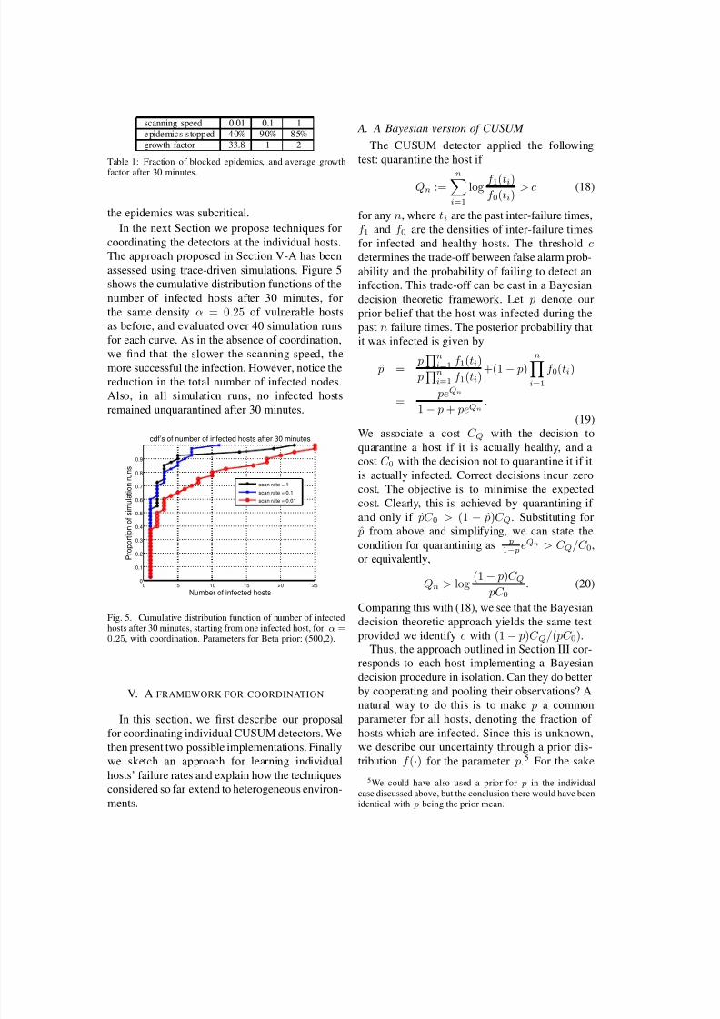
Table 1 provides the fraction of simulation
runs where the worm spread was stopped by 30
minutes, and the average number of infected hosts
among the runs where there still remained infected
hosts (growth factor). These again suggest that the
epidemics was supercritical for a scanning rate of
0.01, with a growth factor of around 34 per 30
minutes, while for scanning rates of 0.1 and 1,
7/30/2019 Efficient Quarantining of Scanning Worms Optimal Detection and Coordination
http://slidepdf.com/reader/full/efficient-quarantining-of-scanning-worms-optimal-detection-and-coordination 10/13
scanning speed 0.01 0.1 1
epidemics stopped 40% 90% 85%
growth factor 33.8 1 2
Table 1: Fraction of blocked epidemics, and average growthfactor after 30 minutes.
the epidemics was subcritical.
In the next Section we propose techniques for
coordinating the detectors at the individual hosts.
The approach proposed in Section V-A has been
assessed using trace-driven simulations. Figure 5
shows the cumulative distribution functions of the
number of infected hosts after 30 minutes, for
the same density α = 0.25 of vulnerable hosts
as before, and evaluated over 40 simulation runs
for each curve. As in the absence of coordination,
we find that the slower the scanning speed, themore successful the infection. However, notice the
reduction in the total number of infected nodes.
Also, in all simulation runs, no infected hosts
remained unquarantined after 30 minutes.
0 5 10 15 20 250
0.1
0.2
0.3
0.4
0.5
0.6
0.7
0.8
0.9
1
Number of infected hosts
P r o p o r t i o n o f s i m u l a t i o n r u n s
cdf’s of number of infected hosts after 30 minutes
scan rate = 1
scan rate = 0.1
scan rate = 0.01
Fig. 5. Cumulative distribution function of number of infectedhosts after 30 minutes, starting from one infected host, for α =
0.25, with coordination. Parameters for Beta prior: (500,2).
V. A FRAMEWORK FOR COORDINATION
In this section, we first describe our proposal
for coordinating individual CUSUM detectors. We
then present two possible implementations. Finally
we sketch an approach for learning individual
hosts’ failure rates and explain how the techniques
considered so far extend to heterogeneous environ-
ments.
A. A Bayesian version of CUSUM
The CUSUM detector applied the following
test: quarantine the host if
Qn :=
ni=1
log f 1(ti)f 0(ti)
> c (18)
for any n, where ti are the past inter-failure times,
f 1 and f 0 are the densities of inter-failure times
for infected and healthy hosts. The threshold cdetermines the trade-off between false alarm prob-
ability and the probability of failing to detect an
infection. This trade-off can be cast in a Bayesian
decision theoretic framework. Let p denote our
prior belief that the host was infected during the
past n failure times. The posterior probability that
it was infected is given by
ˆ p =p
ni=1 f 1(ti)
pn
i=1 f 1(ti)+(1 − p)
ni=1
f 0(ti)
=peQn
1 − p + peQn.
(19)
We associate a cost C Q with the decision to
quarantine a host if it is actually healthy, and a
cost C 0 with the decision not to quarantine it if it
is actually infected. Correct decisions incur zero
cost. The objective is to minimise the expected
cost. Clearly, this is achieved by quarantining if
and only if ˆ pC 0 > (1 − ˆ p)C Q. Substituting for
ˆ p from above and simplifying, we can state thecondition for quarantining as p1− p
eQn > C Q/C 0,
or equivalently,
Qn > log(1 − p)C Q
pC 0. (20)
Comparing this with (18), we see that the Bayesian
decision theoretic approach yields the same test
provided we identify c with (1 − p)C Q/( pC 0).
Thus, the approach outlined in Section III cor-
responds to each host implementing a Bayesian
decision procedure in isolation. Can they do better
by cooperating and pooling their observations? A
natural way to do this is to make p a common
parameter for all hosts, denoting the fraction of
hosts which are infected. Since this is unknown,
we describe our uncertainty through a prior dis-
tribution f (·) for the parameter p.5 For the sake
5We could have also used a prior for p in the individualcase discussed above, but the conclusion there would have beenidentical with p being the prior mean.

7/30/2019 Efficient Quarantining of Scanning Worms Optimal Detection and Coordination
http://slidepdf.com/reader/full/efficient-quarantining-of-scanning-worms-optimal-detection-and-coordination 11/13
of tractability, we take f to be a Beta distribution
with parameters α, β ; that is to say, for p ∈ [0, 1],
f ( p) = f α,β( p) =1
B (α, β )
pα−1(1− p)β−1, (21)
where B (α, β ) is a normalising constant.
Let X i denote the indicator that host i is in-
fected, i.e., X i = 1 if host i is infected and
0 if it is healthy. Now, conditional on p, each
host is assumed to have equal probability p of
being infected, independent of all other hosts.
Next, conditional on X i, the inter-failure times at
host i are assumed to be i.i.d. with distribution
f Xi(·), and independent of inter-failure times at
other hosts. Expressing this formally, the model
specifies the following joint distribution for infec-
tion probability, infection status and inter-failure
times:
f ( p,X, t) = f ( p)N i=1
pXi(1− p)1−Xi
nj=1
f Xi(tij),
(22)
where tij denotes the jth inter-failure time at host
i. From this, we can compute the conditional
distributions of p and X i given the observed inter-
failure times at different hosts.
In the uncoordinated case studied earlier, infer-
ence about X i was based only on observations of
failure times at host i; now, failure times at other
hosts could influence the posterior distribution of X i via their effect on the posterior distribution
of p. Is this desirable? We claim that the answer
is yes; when we have evidence that there is a
worm outbreak in the population, then we should
be more suspicious of unusual failure behaviour
at any individual host. The Bayesian formulation
described above fleshes out this intuition and gives
it a precise mathematical description.
Define
Qin =
nj=1
logf 1(tij)
f 0(tij)(23)
to be the log-likehood ratio of the observed inter-
failure times at host i between the hypotheses that
it is and isn’t infected. We then have:
Proposition 3: The posterior distribution of the
infection probability p is given by
f ( p|t) =1
Z f ( p)
ni=1
1 − p + peQ
in
, (24)
where Z is a normalising constant that does not
depend on p. If f is the Beta distribution (21) and
the parameters α, β are bigger than 1, then the
posterior mode is at the unique solution in (0, 1)of the equation
α − 1
p−
β − 1
1 − p+
N i=1
eQin − 1
(1 − p) + peQin
= 0. (25)
The proof is omitted for lack of space.
Now, conditional on p and the observed failure
times at host j, the posterior probability that X j =1, i.e., that host j is infected, is given, as in (19),
by the expression
P (X j = 1| p, t) =peQ
jn
1 − p + peQjn
.
We can remove the conditioning on p by inte-grating the above expression with respect to the
posterior distribution. However, this is not analyt-
ically tractable. Therefore, we adopt the expedient
of simply replacing p with its posterior mode,
denoted ˆ p and given by the solution of (25). This
can be heuristically justified on the grounds that as
the number of nodes and hence the total number
of observations grows large, the posterior becomes
increasingly concentrated around its mode. Thus,
we rewrite the above as
P (X j = 1|t) ≈ˆ peQ
jn
1 − ˆ p + ˆ peQj
n
,
where ˆ p solves (25). Letting C Q and C 0 denote
the costs of incorrectly quarantining and failing
to quarantine this host respectively, we obtain as
before the Bayes decision procedure: quarantine
host j if and only if
Qjn >
(1 − ˆ p)C Qˆ pC 0
. (26)
Comparing this with (20), we note that the only
difference is that p has been replaced by ˆ p. There-
fore, the decision rule can be implemented by
using a CUSUM detector at each node j, but with
CUSUM threshold cold replaced by
cnew = cold + log1 − ˆ p
ˆ p− log
1 − p
p; (27)
this is clear from (23). Here p denotes the mode
of the prior, which is equal to (α−1)/(α + β −2)for the assumed Beta prior.

7/30/2019 Efficient Quarantining of Scanning Worms Optimal Detection and Coordination
http://slidepdf.com/reader/full/efficient-quarantining-of-scanning-worms-optimal-detection-and-coordination 12/13
B. Implementation
The above scheme requires each host to up-
date its CUSUM threshold based on the revised
estimate ˆ p of the infection probability, that isthe mode of the posterior distribution of p, and
thus the solution of (25). There are a number
of ways that the coordination can be done in
practice: we can have a central node (or chosen
host) receive the CUSUM statistics Qi from the
hosts periodically, calculate ˆ p from (25) and send
this back to the hosts. The numerical calculation
of ˆ p is not expensive, and can be done efficiently
by bisection search, for example.
Alternatively, the hosts are divided into domains
dj , with a leader j responsible for that domain.
Host j periodically collects CUSUM statistics
from its domain, exchanges messages with theother dedicated hosts for producing the revised
estimate ˆ p, and feeds it back to hosts in its domain.
We now describe a strategy for distributed com-
putation of ˆ p among leaders, which does not re-
quire them to broadcast the collection of CUSUM
statistics they are responsible for. Instead, they
broadcast two summary statistics periodically. The
summary statistics for domain j are its size |dj |(in number of hosts) and the following quantity:
sn,j :=
i∈dj pneQ
i
1 − pn + pneQi.
There, pn is the current estimate of ˆ p after ncommunication rounds between leaders. It is up-
dated at each leader after the sn,j’s and |dj |’s are
broadcast according to
pn+1 =α − 1 +
j sn,j
j |dj | + α + β − 2·
It can be shown that under the assumptions
α, β > 1, the iterates pn converge to a fixed point
ˆ p which satisfies (25). As convergence is exponen-
tially fast, only few iterations are needed. Hence
we obtain a significant gain on communication
cost as compared to the centralised approach. Theproof of convergence of the iterative scheme is
omitted due to lack of space.
C. Heterogeneous hosts, unknown parameters
and learning
In the discussion above, the failure time distri-
butions f 1 and f 0 for infected and healthy hosts
p
X1
Λ1
τ11
X2 XN…
Λ2
ΛN…
τ12
τ1n τN1
τ21
τN2
τ22
τ2n τNn
… ……
infection probability
infection status
failure rates
inter-failure times
Fig. 6. Belief network model for inter-failure times.
were assumed to be the same at all hosts, and
to be known. These assumptions were made for
clarity of exposition, but are not necessary. We
now briefly sketch how these assumptions can berelaxed.
In general, each host i can have a different dis-
tribution for inter-failure times, f i0, and a different
distribution for failures caused by a worm f i1. The
framework we use is a Bayesian belief network
where the relationship between the variables is
shown in Figure 6. The top p node in the belief
network of Figure 6 plays the role of correlat-
ing the observations across hosts. If the inter-
failure times distributions f 1, f 0 are taken to be
exponential distributions with parameters λ1, λ0respectively, then the failure rates Λi are just λXi
.
In general there is some uncertainty over the
natural failure rate Λi of the host, and a worm’s
scanning rate. This can be incorporated into the
belief network by assuming that the failure rate
Λi itself is unknown. We assume that, conditional
on the value of X i, it is distributed according to
a Gamma distribution with scale parameter θ and
shape parameter η which depend on the value of
X i. That is to say:
d
dxP(Λi ≤ x|X i) = γ θ(Xi),η(Xi)(x),
where γ θ,η(x) = 1x≥0e−θxθηxη−1 1
Γ(η)
. This
choice of a Gamma prior distribution is made to
ensure tractability of posterior distribution evalu-
ation. Conditional on the parameter Λi, the inter-
failure times τ ij are independent and identically
exponentially distributed with parameter Λ i.
The analysis of Section V-A can be pushed
through. Essentially all the formulas have the same

7/30/2019 Efficient Quarantining of Scanning Worms Optimal Detection and Coordination
http://slidepdf.com/reader/full/efficient-quarantining-of-scanning-worms-optimal-detection-and-coordination 13/13
form, though we have to take expectations over the
unknown parameters. Instead of defining Q in as in
(23) we have
Qin = log
E γ θ(1),η(1)
nj=1 Λie−Λitij
E γ θ0,η(0)
nj=1 Λie
−Λitij
This corresponds to a generalisation of the
CUSUM statistic. In fact with our choice of prior
for Λi this has the explicit form
Qin = log
ρi(1)
ρi(0)(28)
where
ρi(X ) :=θ(X )η(X)Γ(η(X ) + n)
(θ(X ) + S i)n+η(X)Γ(η(X ))
· (29)
and S i :=n
j=1 τ ij .
VI . CONCLUDING REMARKS
In this paper we have used epidemiological
modeling to characterize the interplay between
scanning worms and countermeasures. We have
illustrated this on both existing throttling schemes
and the novel Max-Failure scheme, whose opti-
mality properties have been identified (Proposition
1). We have then identified optimal quarantining
profiles, for which worm spread is independent
of worm scanning speed. This has allowed usto determine simple CUSUM tests that ensure
that worm spread is at most twice as fast as
what an optimal quarantining profile can ensure
(Proposition 2). Our approach to the design of
countermeasures, focusing on the exponent of po-
tential epidemics, allows the derivation of explicit
designs, and thus reduces the number of free
parameters to be configured.
We have proposed a Bayesian approach for
combining individual detectors and hence speed
up reaction of such detectors to worms. The
uncoordinated and coordinated approaches have
been evaluated using trace-driven simulations. The
experimental results indicate that the proposed
countermeasures can be efficient in environments
such as the corporate research lab where the
trace has been collected. We intend to experiment
our proposals in different environments, target-
ting more particularly home users. We also plan
to evaluate more thoroughly the Bayesian ap-
proach for learning individual host characteristics
sketched in Section V-C.
REFERENCES
[1] S. Asmussen, Applied Probability and Queues. Springer-Verlag, 2003.
[2] F. Baccelli and P. Brémaud, Elements of Queueing The-
ory. Springer-Verlag, 2003.[3] C.-S. Chang, Performance Guarantees in Communication
Networks, Springer, 2000.[4] M. Costa, J. Crowcroft, M. Castro, A. Rowstron, L.
Zhou, L. Zhang, and P. Barham. Vigilante: End-to-EndContainment of Internet Worms. In Proc. SOSP 2005,Brighton, United Kingdom, October 2005.
[5] D.J. Daley and J. Gani, Epidemic Modelling: An Intro-duction, Cambridge University Press, 1999.
[6] J. Jung and V. Paxson and A. Berger and H. Balakrishnan,Fast portscan detection using sequential hypothesis test-ing, In Proc. IEEE Symposium on Security and Privacy,
May 9– 12, 2004.[7] H.A. Kim and B. Karp, Autograph: toward automated,distributed worm signature detection. In Proc. 13thUSENIX Security Symposium, August 2004.
[8] J.-Y. Le Boudec and P. Thiran, Network Calculus,Springer, 2001.
[9] G. Moustakides, Optimal procedures for detectingchanges in distributions. Annals of Statistics, vol. 14, pp.137-1387, 1986.
[10] D. Moore, V. Paxson, S. Savage, C. Shannon, S. Stanifordand N. Weaver, Inside the Slammer Worm. IEEE Securityand Privacy, 1(4), pp. 33-39, 2003.
[11] D. Moore, C. Shannon and J. Brown, Code-Red: a casestudy on the spread and victims of an Internet Worm. InProc. ACM/USENIX Internet Measurement Workshop,2002.
[12] Y. Ritov, Decision theoretic optimality of the CUSUM
procedure, Annals of Statistics, vol. 18, pp. 1464-1469,1990.[13] S.E. Schechter, J. Jung and A.W. Berger, Fast Detection
of Scanning Worm Infections, 7th International Sympo-sium on Recent Advances in Intrusion Detection (RAID),2004.
[14] A. Shwartz and A. Weiss, Large Deviations for Perfor-mance Analysis, Chapman&Hall, London, 1995.
[15] J. Twycross and Matthew Williamson, Implementing andtesting a virus throttle, In Proc. 12th USENIX SecuritySymposium, USENIX, 2003.
[16] N. Weaver, V. Paxon, S. Staniford and R. Cunningham, Ataxonomy of computer worms. In Proc. ACM workshopon Rapid Malcode (WORM), 2003.
[17] M. M. Williamson, Throttling Viruses: Restricting Prop-agation to Defeat Mobile Malicious Code. In ACSAC,2002.
[18] C. Zou, L. Gao, W. Gong and D. Towsley, Monitoringand Early Warning for Internet Worms, In Proc. of the10th ACM Conference on Computer and Communica-tions Security, pp. 190-199, 2003.