ELSEVIER

Science of Computer Programming

Science of Computer programming 23 ( 1994) 1-18

Efficient parallel algorithms for tree accumulations

Jeremy Gibbons a,*, Wentong Cai b, David B. Skillicornc a Department of Computer Science, Universiv of Auckland, Private Bag 92019, Auckland, New Zealand

b School of Applied Science, Nanyang Technological University, Singapore 2263, Singapore ’ Department of Computing and Information Science, QueenS Universi& Kingston, Ont. K7L 3N6, Canada

Received March 1993; revised April 1994; communicated by R. Bird

Abstract

Accumulations are higher-order operations on structured objects; they leave the shape of an object unchanged, but replace elements of that object with accumulated information about other elements. Upwards and downwards accumulations on trees are two such operations; they form the basis of many tree algorithms. We present two EREW PRAM algorithms for computing accumulations on trees taking 0( log n) time on 0( n/ log n) processors, which is optimal.

1. Introduction

Accumulations are higher-order operations on structured objects that leave the shape

of an object unchanged, but replace every element of that object with some accumulated

information about other elements. For example, the prefb sums or scan operation [ 31 on

lists that, for an associative operator 0, maps the list [al, . . . , a,,] to the list of “partial

sums”

[al, alOa2, . . . . alOa20+..0a,]

is an accumulation: it replaces each element of the list with the “sum” of the elements

to its left. Another way of saying this is that information is “passed along the list”, from

left to right.

This paper concerns two kinds of accumulation on binary trees, upwards and down- wards accumulation. Upwards accumulation passes information up through a tree, from

the leaves towards the root; each element is replaced by some function of its descendants, that is, of the elements below it in the tree. Symmetrically, downwards accumulation

*Corresponding author. E-mail: jeremy@cs.aukuni.ac.nz.

0167-6423/94/$07.00 @ 1994 Elsevier Science B.V. All rights reserved SSDIO167-6423(94)00013-5

2 J. Gibbons et al. /Science of Computer Programming 23 (1994) 1-18

passes information downwards, from the root towards the leaves; each element is re-

placed by some function of its ancestors, that is, of the elements above it in the tree.

Upwards and downwards accumulations form the basis of many important algorithms,

and so are a useful idiom to add to the programmer’s toolbox. For example, computing

the sizes of subtrees and the depths of nodes are natural applications of upwards and

downwards accumulation, respectively. The parallel prefix algorithm [ lo] for computing

the prefix sums of a list in logarithmic time on linearly many processors involves building

a tree with the list elements as leaves, then performing an upwards and downwards

accumulation on the tree [7]; the prefix sums problem in turn has applications in

the evaluation of polynomials, compiler design, and numerous graph problems including

minimum spanning tree and strongly connected components [ 2 1. Upwards accumulation

can be used to solve some optimization problems on trees, such as minimum covering

set and maximal independent set [9]. Other algorithms such as Reingold and Tilford’s

algorithm [ 121 for drawing trees and a two-pass algorithm for completely labelling a

tree according to an attribute grammar [6] also consist of an upwards followed by a

downwards accumulation.

For a tree with n elements, these accumulations can be computed naively on a

sequential machine in time proportional to n, and on a parallel machine with n processors

in time proportional to the depth of the tree. We show here how to adapt Abrahamson

et al.‘s parallel tree contraction algorithm [ l] for computing tree reductions to allow

the accumulations to be computed in logarithmic time on an n-processor EREW PRAM,

even if the tree has greater than logarithmic depth. Straightforward application of Brent’s

Theorem [4] reduces the processor usage to n/ log n, which gives optimal algorithms.

The remainder of this paper is organized as follows. In Section 2 we give the defini-

tions of tree reductions and of upwards and downwards accumulations. In Section 3 we

review parallel tree contraction. In Sections 4 and 5 we adapt the contraction algorithm

to computing upwards and downwards accumulations, respectively.

2. Upwards and downwards accumulations

Our binary trees have labels drawn from two sets: leaf labels are drawn from a set A

and junction labels from a set 8. A binary tree is either a leaf, labelled with an element

of A, or a junction with two children, labelled with an element of B. Thus, we have no

empty tree and every parent has exactly two children.

The @-reduction of a tree for a ternary operator @ from A x B x A to A reduces a

binary tree to a single value in A. For example, the @-reduction of the tree in Fig. 1,

where a, c E B and b, d, e E A, is the single value bOa (d&e) in A. Note that the ternary

operator is written with its middle argument as a subscript. (A more general form of

reduction-in fact, a homomorphism-can be obtained by first mapping a function f of

type A -+ C for some third type C over the leaves, and returning a single value in C; the

discussion in the rest of this paper can easily be generalized to such homomorphisms.)

Tree reductions can be computed naively on a sequential machine in time proportional

J. Gibbons et al. /Science of Computer Programming 23 (I 994) l-18 3

Fig. I. A binary tree.

Fig. 2. The @-upwards accumulation of the tree in Fig. 1.

to the size of the tree and on a parallel machine with n processors in time proportional

to the depth of the tree, if the operator @ takes constant sequential time. (For the rest

of the paper, we assume that “component” operators like 0 take constant time.) Under

certain conditions on 0, the parallel contraction algorithm reviewed in the next section

reduces this to logarithmic parallel time even if the tree has greater than logarithmic

depth.

Upwards accumulations generalize reductions; instead of computing a single value,

an upwards accumulation computes a tree of partial results with the same shape as its

argument-each node is labelled with the reduction of the subtree originally rooted at

that node. For example, the @-upwards accumulation of the tree in Fig. 1 is shown in

Fig. 2. Notice that an upwards accumulation returns a honzogeneous tree, that is, one in

which leaf and junction labels have the same type.

Upwards accumulations can be computed naively with the same amount of work as

reductions, since the partial results must be computed anyway. It is significant, though,

that an upwards accumulation consists of applying a reduction, as opposed to just any

function, to all subtrees. Were this not the case, it would not be possible to compute

the value for a parent from the values for its children-put another way, the required

“partial results” would not be byproducts of the naive computation of the reduction.

A downwards accumulation also computes a tree of values with the same shape as its

argument; each node is labelled with a path reduction of the elements on the path from

the root of the tree to that node. For two binary operators @ and @ which cooperate

[ 81, that is, which satisfy the four laws

a@(b@c)=(a@b)@c

a@(b@c)=(a@b)@c

a@(b@c)=(a@b)@c

a@(b@c)=(a@b)mc

(1)

A J. Gibbons et al/Science of Computer Programming 23 (1994) I-18

Fig. 3. The path to the element d in the tree in Fig. 1.

Fig. 4. The (@, @)-downwards accumulation of the tree in Fig. 1.

the (@, 8) -path reduction consists of replacing all “left turns” with @ and all “right

turns” with @. For example, Fig. 3 shows the path to the element labelled d in the

tree in Fig. 1; the reduction of this path is a @ c 6~ d. Because of cooperativity, no

parentheses are needed in this expression. Note also that a consequence of cooperativity

is that ~3 and @ must each have type A x A 4 A; downwards accumulations can only

be performed on homogeneous trees.

The (@, @)-downwards accumulation of a tree consists of replacing every element

with the (@, @)-path reduction of the path to that element. For example, Fig. 4 shows

the accumulation of the tree in Fig. 1. Again, the result is a homogeneous tree.

3. Parallel tree contraction

Our algorithms for computing accumulations on trees are modifications of parallel

tree contraction algorithms [ 1,111, which reduce a tree to a single value. We present

here a description of parallel tree contraction which we generalize later to the algorithms

for accumulation.

We suppose that a binary tree with n nodes is represented as a collection of n

processors. Each processor u maintains a number of variables: u.j is a boolean, and is

true iff u is a junction; u.p is a pointer to the parent of u; us is a boolean, and is true

iff u is the left child of its parent (the “s” stands for “side”). We suppose that root is a

pointer to the root of the tree, and to avoid special cases we suppose that root.p points

somewhere, and that root.p.1 = root and roots is true, so that the root is “the left child

of its parent”. If u.j is false, u has the variable u.a E A, a “leaf label”; otherwise, u has

the variable u.b E B, a “junction label”. If u.j is true, u also has the extra variables u.l

and u.r, being pointers to its left and right children. Finally, every processor u has a

variable u.g, an “auxiliary function” from A to A. This auxiliary function can be thought

of as labelling the edge between u and u.p and affecting the computation of the tree

J. Gibbons et al./Science of Computer Programming 23 (1994) l-18 5

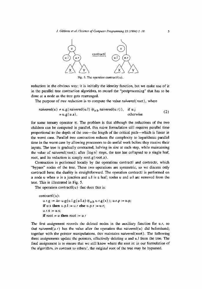
contractl, d u

0 Lt.1 u.r AL X Y

Fig. 5. The operation contractl( u).

reduction in the obvious way; it is initially the identity function, but we make use of it

in the parallel tree contraction algorithm, to record the “postprocessing” that has to be

done at a node as the tree gets rearranged.

The purpose of tree reduction is to compute the value naivered( root), where

naivered( u) = u.g( naivered( u.1) @&b naivered(u.r)), if u.j

= u.g( u.a), otherwise (2)

for some ternary operator 0. The problem is that although the reductions of the two

children can be computed in parallel, this naive formulation still requires parallel time

proportional to the depth of the tree-the length of the critical path-which is linear in

the worst case. Parallel tree contraction reduces the complexity to logarithmic parallel

time in the worst case by allowing processors to do useful work before they receive their

inputs. The tree is gradually contracted, halving in size at each step, while maintaining

the value of naivered( root) ; after [log n] steps, the tree has collapsed to a single leaf,

root, and its reduction is simply root.g( roota).

Contraction is performed locally by the operations contract1 and contra&, which

“bypass” nodes of the tree. These two operations are symmetric, so we discuss only

contract1 here; the duality is straightforward. The operation contract1 is performed on

a node u when u is a junction and u.l is a leaf; nodes u and u.l are removed from the

tree. This is illustrated in Fig. 5.

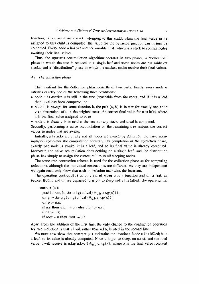
The operation contract1 (u) that does this is:

contractl( u):

u.r.g := Ax’u.g(u.l.g(u.1.a) 6&b u.r.g(x)); u.r.p := u.p;

if us then u.p.1 := u.r else u.p.r := u.r;

u.r.s := u.s;

if root = u then root := u.r

The first assignment records the deleted nodes in the auxiliary function for u.r, so

that naivered( u.r) has the value after the operation that naivered did beforehand;

together with the pointer manipulations, this maintains naivered( root). The following

three assignments update the pointers, effectively deleting u and u.l from the tree. The

final assignment is to ensure that we still know where the root is: in our formulation of

the algorithm, in contrast to others’, the original root of the tree may be bypassed.

6 J. Gibbons et al. /Science of Computer Programming 23 (1994) 1-18

These contraction operations each remove two nodes, one of which is a leaf. Abraham-

son et al. [ 11 present a simple scheme by which many such contraction operations-in

fact, half as many as there are leaves-can be performed in just two steps, without

mutual interference. Their scheme is as follows:

(i) Assume all leaves are numbered from left to right, starting with zero. This

numbering is easily computed in O( log n) time on 0( n/ log n) processors [ 51.

(ii) Mark all even-numbered leaves.

(iii) For every junction u such that u.I is a marked leaf, perform contractl( u).

(iv) For every junction u not involved in the previous step such that u.r is a marked

leaf, perform contractr( u).

(v) Renumber the leaves by halving their numbers.

Actually, Abrahamson et al. mark the odd-numbered leaves; marking the even-numbered

leaves instead sometimes reduces the size of the tree by an extra element. Note also that

the operations contract.1 and contractr are never performed concurrently; the reason for

this is explained later.

Clearly, this scheme deletes at least half of the leaves, but we must show that no

concurrent contraction operations interfere.

Note that the operation contractl( u) involves nodes on three consecutive levels, u.p, u

and u.r; however, the fields of u.p and u.r that are involved are disjoint, so contractions

involving nodes two (or more) levels apart do not interfere. Contractions involving two

nodes on the same level do not interfere: the children of the two nodes are disjoint,

and the nodes can at worst be left and right children of the same parent. Only nodes

on adjacent levels remain to be considered. If neither of the two nodes is the parent of

the other, they do not interfere, so suppose that one is the parent of the other. The two

will only be contracted simultaneously if they both have marked leaves as (without loss

of generality) left children-but such leaves are adjacent in left-to-right order, and so

cannot both be even-numbered. Hence, a node and its parent will not be simultaneously

contracted, and consequently no concurrent contraction operations interfere.

Only one aspect is left to consider: the contraction steps must take constant time, but

the contraction operations assign lambda expressions of increasing size to the auxiliary

functions. We must ensure that the time taken to compute new lambda expressions from

old remains constant no matter what lambda expressions are generated at intermediate

steps, and despite the fact that they appear to grow in size (and might therefore require

longer times to access and manipulate). One way to ensure this is to use indices into

a set of lambda expressions in place of the lambda expressions themselves. Then the

requirement that each contraction step takes constant time is met if the indexed sets

meet the following conditions:

l for every u, the “sectioned” binary operator @u.b from A x A to A and the function

u.g are drawn from indexed sets of functions F and G (which contains the identity

function) respectively;

l functions in F and G can be applied in constant time;

l for all @ E F, g E G and a E A, the functions Ax.g(x) @a and hx. a @g(x) are both

in G, and their indices can be computed from a and from the indices of 0 and g in

J. Gibbons et al./Science of Computer Programming 23 (1994) I-18

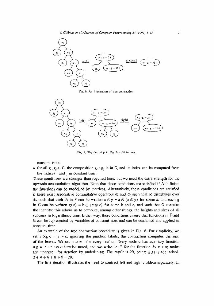
Fig. 6. An illustration of tree contraction.

right U) : g = 2+ &% i!? u* g = 15+

Fig. 7. The first step in Fig. 6, split in two.

constant time;

l for all gi, gj E G, the composition gi o gj is in G, and its index can be computed from

the indices i and j in constant time.

These conditions are stronger than required here, but we need the extra strength for the

upwards accumulation algorithm. Note that these conditions are satisfied if A is finite:

the functions can be modelled by matrices. Alternatively, these conditions are satisfied

if there exist associative commutative operators @ and @ such that @ distributes over

@, such that each 0 in F can be written x 0 y = a @ (x $ y) for some a, and each g

in G can be written g(x) = b @ (c @ x) for some b and c, and such that G contains

the identity; this allows us to compute, among other things, the heights and sizes of all

subtrees in logarithmic time. Either way, these conditions ensure that functions in F and

G can be represented by variables of constant size, and can be combined and applied in

constant time.

An example of the tree contraction procedure is given in Fig. 6. For simplicity, we

set a @b c = a + c, ignoring the junction labels; the contraction computes the sum

of the leaves. We set ui.a = i for every leaf ui. Every node u has auxiliary function

u.g = id unless otherwise noted, and we write “c+” for the function Ax.c + x; nodes

are “marked” for deletion by underlining. The result is 29, being ia.g( U8.a); indeed,

2+4+6+8+9=29.

The first iteration illustrates the need to contract left and right children separately. In

8 .I. Gibbons et al/Science of Computer Programming 23 (1994) 1-18

Fig. 7, we split this step in two, contracting first u1 and us, whose left children are

marked, and then ~7, whose right child is marked. The function 15+ assigned to ua.g

in the second half is (6 + 9>+, and depends on the function 6+ assigned to u7.g in the

first half.

Thus, in constant time on an n processor EREW PRAM we can delete half of the

leaves while maintaining naivered( root), so in O(logn) time we can reduce the tree to

a single leaf and thereby compute the tree reduction. A straightforward application of

Brent’s Theorem reduces the number of processors to O( n/ log n), which gives optimal

efficiency.

4. Parallel upwards accumulation

The parallel tree contraction algorithm can be used to compute the upwards accumu-

lation, in which not only the final result but also all intermediate results are computed.

In essence, whenever a node u is deleted from the tree, it is placed on a stack maintained

by its remaining child; after this child receives its final value, it unstacks u and computes

the final value of u too.

We assume that every node u has an extra variable, u.val; the purpose of the upwards

accumulation is to compute u.val for every u, the required values being those given by

the sequence

initialize; naiveua (root)

where

initialize :

for each node u do in parallel u.g := id;

for each node u do in parallel if 7u.j then u.val := u.a

and

naiveua (u) ;

if u .j then begin

do in parallel begin

naiveua( u.1) 0 naiveua( u.r)

end; u.val := u.l.g(u.l.val) @&,b u.r.g(u.r.val)

end

(The “ Cl ” is parallel, as opposed to sequential, composition.) The problem is that, as

for reduction, naiveua has a critical path as long as the tree is deep.

To get around this problem, we use tree contraction as before. Each contraction

bypasses two nodes in the tree, one a leaf and one a junction. The final value to be

assigned to the junction is not yet known, but it is some known function of the final

value to be assigned to its remaining child. The bypassed junction, together with this

J. Gibbons et al. /Science of Computer Programming 23 (1994) l-18 9

function, is put aside on a stack belonging to this child; when the final value to be

assigned to this child is computed, the value for the bypassed junction can in turn be

computed. Every node u has yet another variable, ust, which is a stack to contain nodes

awaiting their final values.

Thus, the upwards accumulation algorithm operates in two phases, a “collection”

phase in which the tree is reduced to a single leaf and some nodes are put aside on

stacks, and a “distribution” phase in which the stacked nodes receive their final values.

4.1. The collection phase

The invariant for the collection phase consists of two parts. Firstly, every node u

satisfies exactly one of the following three conditions:

l node u is awake: u is still in the tree (reachable from the root), and if it is a leaf

then u.val has been computed, or

l node u is asleep: for some function h, the pair (u, h) is in v.st for exactly one node

v (a descendant of u in the original tree) ; the correct final value for u is h(x) where

x is the final value assigned to v, or

l node u is dead: u is in neither the tree nor any stack, and u.val is computed.

Secondly, performing a naive accumulation on the remaining tree assigns the correct

values to nodes that are awake.

Initially, all stacks are empty and all nodes are awake; by definition, the naive accu-

mulation completes the computation correctly. On completion of the collection phase,

exactly one node is awake: it is a leaf, and so its final value is already computed.

Moreover, the naive accumulation does nothing on a single leaf, and the distribution

phase has simply to assign the correct values to all sleeping nodes.

The same tree contraction scheme is used for the collection phase as for computing

reductions, although the individual contractions are different. As they are independent

we again need only show that each in isolation maintains the invariant.

The operation contractl(u) is only called when u is a junction and u.l a leaf, as

before. Both u and u.l are bypassed; u is put to sleep and u.l is killed. The operation is:

contractI(

push(u.r.st, (u, Ax.u.l.g(u.l.val) @“,b u.r.g(x)));

u.r.g := hx.u.g(u.l.g(u.l.val) @&b u.r.g(X));

u.r.p := u.p;

if u.s then u.p.1 := u.r else u.p.r := u.r;

u.r.s := u.s;

if root = u then root := u.r

Apart from the addition of the first line, the only change to the contraction operation

for tree reduction is that u.l.val, rather than u.l.a, is used in the second line.

We must now show that contractl(u) maintains the invariant. Node u.l is killed; it is

a leaf, so its value is already computed. Node u is put to sleep, on u.r.st, and the final

value it will receive is u.l.g(u.l.val) @“,b u.r.g(x), where x is the final value received

10 J. Gibbons et al. /Science of Computer Programming 23 (1994) l-l 8

by u.r; clearly, this value is what the naive accumulation would have given it. The

assignment to u.r.g thus ensures that the values given by the naive accumulation to the

ancestors of u remain unchanged, as are the values given to descendants of u.r and all

unrelated nodes. Hence the invariant is maintained.

Because the same contraction scheme is used as for tree reduction, the collection

phase takes O(log n) steps.

To illustrate the process, consider the example of tree contraction given earlier. The

corresponding accumulation computes for each node u the sum of the leaves of the

subtree rooted at u. At each contraction operation, one leaf is killed-being a leaf, its

final value is already computed-and one junction is put to sleep. After the first iteration,

ug.st contains (IQ, 2+), u7st contains (u5,6+) and u3.st contains (u7,9+); after the

second iteration, u5.st grows to contain (u3,4+ o 15-F = 19+). Thus, on completion of

the collection phase, the status of the stacks is

ug.st u7 .st U8 .st

(u1,2+) (u5,6+) (u3,19+)

(u7,9+)

so t.11, ~3, u5 and u7 (the junctions) are sleeping, UI3 is still awake, and the remaining

leaves are dead; all the leaves, of course, already have their final values.

4.2. The distribution phase

Every node u has a stack u.st of (node, function) pairs; if (v, h) is in u.st then

v.val should be set to h(u.val), once u.val has been computed. The distribution phase

is simply:

for each node u do in parallel begin

wait until u.val is computed;

while ust not empty do begin

(v, h) := pop(u.st);

v.val := h( u.val)

end

end

Clearly this terminates: there are no circular dependencies, because all dependencies run

from parents to children. Clearly, also, when it terminates every node has the correct

value assigned to it, by virtue of the invariant for the collection phase. We show now

that the distribution phase also terminates in O(log n) steps.

Define dep(v) for a node v that has been put to sleep to be the node whose stack

contains v-that is, v is in dep(v) st. During the collection phase, dep(v) may itself be

put to sleep, as may dep(dep(v)), and so on. Define the dependency chain of v at a

particular point during the collection phase to be the sequence vu, VI, . . . , vk such that

vo = V, Vi = dep(vi_1) for 1 < i < k, and dep(vk) is not asleep. Write Id(v) for vk,

the last sleeping node on whose final value v depends, and src( v) for dep( Id (v) > , the

J. Gibbons et al. /Science of Computer Programming 23 (1994) I-18 11

non-sleeping node on whose final value v depends. Write sd(v) for the depth of v in

dep(v).st, counting the top of the stack as depth 1.

For every node v, define the dependency depth dd(v) of v at a particular point during

collection as sd(v) + sd(dep(v)) +. +. + sd( Id( v) >, the sum of the stack depths of

all nodes in the dependency chain of v. (If v is not asleep, sd(v) = 0.) For example,

after the first iteration of the collection phase in the example, UT is at the top of LQ.St

and u5 is at the top of uT.st, so sd(u7) = 1 and sd(ug) = 1, and dd(u5) = 2. We

claim that at all points during the collection phase, dd(v) is bounded above by twice

the number of iterations that have been made, and after dd(v) steps of the distribution

phase v will receive its final value. Hence, dd(v) is bounded above overall by 2 log n,

and the distribution phase takes at most 2 log n steps.

Consider a node v and the contraction of left children during one iteration of the

collection phase. The node src(v) is either awake or dead. If src(v) is dead, the

dependency depth of v doesn’t change. If src(v> is awake, it may be put to sleep, in

which case the dependency chain of v grows by one element, and dd(v) increases by

one. Alternatively, the parent of src(v) may be put to sleep, in which case src(v) .st

grows by one element, and sd( Id( v) ) and hence dd( v) increase by one. Otherwise,

dd(v) does not change. Thus, dd(v) increases by at most one during the contraction

of left children in one iteration of the collection phase. Similarly, dd(v) increases by at

most one during the contraction of right children. Thus, dd(v) increases by at most two

on each iteration of the collection phase.

During the distribution phase, src(v) .val has been computed for every sleeping node

v. On each iteration of the distribution phase, the top node in src(v> .st is popped and

its final value computed, and so sd( Id(v)) and hence dd(v) decrease by one. If Id(v)

was at the top of src(v).st, that is, sd(ld(v)) = 1, then this computes Id(v).val, at

which point the dependency chain for v shortens by one element; src(v) becomes what

Id(v) used to be. (No assignments are involved; the names Id(v) and src(v) are purely

for expository purposes.) When dd(v) reaches one, Id(v) = v and v is the top element

in src(v) .st, and v.val can be computed. Hence, v.val is computed after exactly dd(v)

iterations of the distribution phase; final values of nodes are “filled in” in the reverse of

the order in which those nodes were stacked.

Returning to our example, ug.Val = 8 is known immediately on completion of the

collection phase, so Ug.st is popped and ug.val = 19 + 8 = 27 is computed. Next, ug.st

and again Ug.st are popped, and ul.val = 2 + 27 = 29 and q.val = 9 + 8 = 17 are

computed. Finally, u7.s.t is popped and ug.val = 6 + 17 = 23 computed.

5. Parallel downwards accumulation

The downwards accumulation likewise operates in two phases, collection and distri-

bution. However, it is more natural to express the contraction operations for downwards

accumulation in terms of parents bypassing children, rather than children bypassing

parents. To this end we reformulate the parallel tree contraction algorithm to use this

12 J. Gibbons et al. /Science of Computer Programming 23 (1994) l-18

method, before adapting the algorithm to downwards accumulation. Then the major

change is that the two children of a junction, at least one of which is a leaf, are by-

passed simultaneously, and both must be placed on the parent’s stack, because the final

values of both depend on the final value of the parent.

The purpose of downwards accumulation is to compute uval for every u, the required

values being those given by

initialize; naiveda(id, root)

where

initialize:

for each node u do in parallel u .g := id

and

naiveda(h, u):

u.val := h(u.a);

if u.j then do in parallel begin

naiveda( Ax. u.g(u.val) CB x, u.1) 0

naiveda(Ax. u.g(u.val) @IX, u.r)

end

(Since downwards accumulations can only be performed on homogeneous trees, we

suppose that, for a downwards accumulation, every processor u has a variable u.a,

regardless of whether u.j is true or false, and that none has a variable u. b.) As with tree

reduction and upwards accumulation, the naive downwards accumulation algorithm has

a critical path as long as the tree is deep, and the point of the exercise is to compute

the accumulation in logarithmic time regardless of the depth.

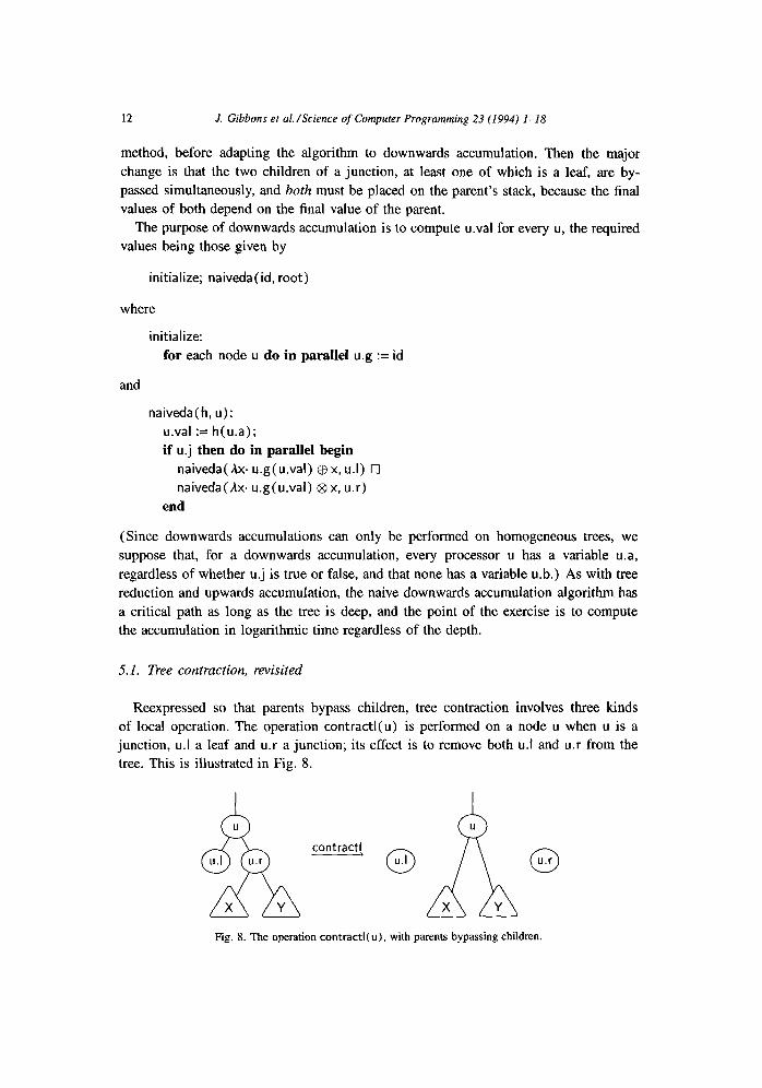
5.1. Tree contraction, revisited

Reexpressed so that parents bypass children, tree contraction involves three kinds

of local operation. The operation contractl(u) is performed on a node u when u is a

junction, u.l a leaf and u.r a junction; its effect is to remove both u.l and u.r from the

tree. This is illustrated in Fig. 8.

contract1

0 u.I 0 u.r

Fig. 8. The operation contractl( u), with parents bypassing children.

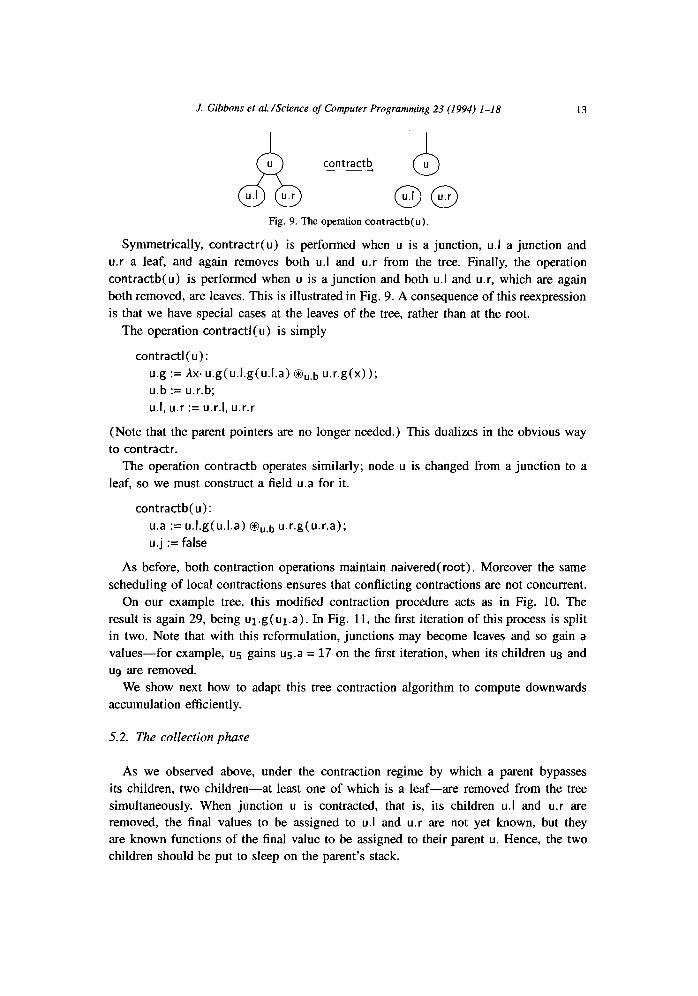
J. Gibbons et al./Science of Computer Programming 23 (1994) I-18 13

J II

Fig. 9. The operation contractb(u).

Symmetrically, contra&(u) is performed when u is a junction, u.l a junction and

u.r a leaf, and again removes both u.l and u.r from the tree. Finally, the operation

contractb(u) is performed when u is a junction and both u.I and u.r, which are again

both removed, are leaves. This is illustrated in Fig. 9. A consequence of this reexpression

is that we have special cases at the leaves of the tree, rather than at the root.

The operation contractl( u) is simply

contract1 (u) :

u.g := AX.U.g(U.l.g(U.l.a) @“,b U.r.g(X));

u.b := u.r.b;

u.1, u.r := u.r.1, u.r.r

(Note that the parent pointers are no longer needed.) This dualizes in the obvious way

to contra&.

The operation contractb operates similarly; node u is changed from a junction to a

leaf, so we must construct a field u.a for it.

contractb( u):

u.a := u.i.g(u.1.a) @“,b U.r.g(u.r.a);

u.j := false

As before, both contraction operations maintain naivered(root). Moreover the same

scheduling of local contractions ensures that conflicting contractions are not concurrent.

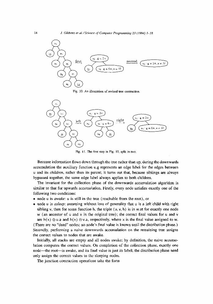
On our example tree, this modified contraction procedure acts as in Fig. 10. The

result is again 29, being ul.g(u1.a). In Fig. 11, the first iteration of this process is split

in two. Note that with this reformulation, junctions may become leaves and so gain a

values-for example, ug gains u5.a = 17 on the first iteration, when its children ua and

ug are removed.

We show next how to adapt this tree contraction algorithm to compute downwards

accumulation efficiently.

5.2. The collection phase

As we observed above, under the contraction regime by which a parent bypasses

its children, two children-at least one of which is a leaf-are removed from the tree

simultaneously. When junction u is contracted, that is, its children u.I and u.r are

removed, the final values to be assigned to u.I and u.r are not yet known, but they

are known functions of the final value to be assigned to their parent u. Hence, the two

children should be put to sleep on the parent’s stack.

J. Gibbons et d/Science of Computer Programming 23 (1994) 1-18

Fig. 10. An illustration of revised tree contraction.

Fig. 11. The first step in Fig. 10, split in two.

Because information flows down through the tree rather than up, during the downwards

accumulation the auxiliary function u.g represents an edge label for the edges between

IJ and its children, rather than its parent; it turns out that, because siblings are always

bypassed together, the same edge label always applies to both children.

The invariant for the collection phase of the downwards accumulation algorithm is

similar to that for upwards accumulation. Firstly, every node satisfies exactly one of the

following two conditions:

l node u is awake: u is still in the tree (reachable from the root), or

l node u is asleep: assuming without loss of generality that u is a left child with right

sibling v, then for some function h, the triple (u, v, h) is in wst for exactly one node

w (an ancestor of u and v in the original tree) ; the correct final values for u and v

are h(x) $ u.a and h(x) &v.a, respectively, where x is the final value assigned to w.

(There are no “dead” nodes; no node’s final value is known until the distribution phase.)

Secondly, performing a naive downwards accumulation on the remaining tree assigns

the correct values to nodes that are awake.

Initially, all stacks are empty and all nodes awake; by definition, the naive accumu-

lation computes the correct values. On completion of the collection phase, exactly one

node-the root-is awake, and its final value is just its label; the distribution phase need

only assign the correct values to the sleeping nodes.

The junction contraction operations take the form

J. Gibbons et al./Science of Computer Programming 23 (1994) 1-18 15

contractl( u):

push(u.st, (u.1, u.r, u.g));

u.g := Ax.u.r.g(u.g(x) @ u.r.a);

u.1, u.r := u.r.1, u.r.r

To show that this maintains the invariant, we must show that the triple pushed onto ust

provides the correct final values for u.l and u.r, the two nodes put to sleep, and that

the contraction does not change the values assigned by the naive accumulation to the

nodes remaining awake. The first requirement is met by virtue of the invariant for the

collection phase. For the second, we note that only descendants of u may be affected

by the contraction, because the naive accumulation passes information downwards. The

value given to u itself is unaffected. The assignment to u.g ensures that the values given

to the (new) children of u are unaffected, and hence so are the values given to all

further descendants of u.

Leaf contraction is simpler:

contractb( u):

push(u.st, (u.l,u.r, u.g));

u.j := false

The argument for the maintenance of the invariant is correspondingly simpler. The

two children of u are put to sleep with the correct function, for the same reason as

for junction contraction, and the values given to the remaining awake nodes are all

unaffected, because none are descendants of u.

Using the same global scheduling scheme, the collection phase takes O(logn) steps.

Again, we have to show that as the auxiliary functions “grow” to record more deleted

nodes, they do not take longer to apply. This is the case if the following conditions are

satisfied:

l the auxiliary functions are drawn from an indexed set G of functions, containing the

identity function;

l functions in G can be applied in constant time;

l for all functions gi, gj E G and labels a E A, the two functions gi 0 (AX. x @ a) o gj

and gi o (Ax.x @ a) o gj are in G, with indices that can be computed from i, j and a

in constant time.

This in turn is satisfied if the set G consists of the identity function and all functions of

the form (Ax. x @ a) and (Ax. x @ a), and A is finite. Alternatively, the finiteness of A

can be replaced by the condition that the operators CB and @ cooperate; this allows us

to compute the depth of every node, among other things, in logarithmic time.

To illustrate this, consider the downwards accumulation in which @ = @ = + on a

tree of the same shape as before, but in which both leaves and junctions have a values;

again, ui.a = i for each i. The accumulation computes for each node u the sum of the

values on the path from the root of the tree to u. The two iterations are illustrated in

Fig. 12. Fig. 13 dissects the first iteration to reveal the intermediate step. After the first

half of the first iteration, ul.st contains (~2, u3, id) and us.st contains (4, u7, id); after

16 J. Gibbons et al. /Science of Computer Programming 23 (1994) I-I 8

second

Fig. 12. An illustration of computing a downwards accumulation.

right -

Fig. 13. The first step in Fig. 12, split in two.

the second half, the extra triple (ug, ug, f7) is pushed onto ug.st. After the second and final iteration, ~1st gains (u4,ug, +3). Thus, the status of the stacks on completion of the collection phase is

Ul St.

(u4, tJ5, -i-3) (uz, ~3, id)

u5.st

(u8, U9, +7) (US, ~7, id)

5.3. The distribution phase

Every junction u has a stack u.st of (node, node, function) triples; if (v, w, h) is in ust then v.vai should be set to h(u.val) CB v.a and w.val to h(u.vai) @ w.a, once u.val has been computed. The distribution phase is simply

for each node u do in parallel begin wait until u.val is computed; while ust not empty do begin

(v, w, b) := pop{ u.st); v.val, w.val := h(u.val) CB v.a, h(u.val) @ w.a

end end

J. Gibbons et al. /Science of Computer Programming 23 (1994) I-18 17

The argument about dependency depths remains the same; the dependency depth dd(v)

for each node v is bounded above by twice the number of iterations of the collection

phase, and hence by 2 log n, and each sleeping node v receives its final value after dd( v)

steps of the distribution phase.

In our example, initially ul.val = u1.a = 1 is computed. Then u1.s.t is popped and

u4.val = 1 + 3 + 4 = 8 and us.val = 1 + 3 + 5 = 9 are computed. Then ugst and again

ulst are popped, and IJ8.d = 9+7+8 = 24, ug.val= 9+7+9 = 25, u2.val = 1+2 = 3

and ug.val = 1 + 3 = 4 computed. Finally, u5.st is popped again and Us.val = 9 + 6 = 15

and u7.val= 9 + 7 = 16 are computed.

6. Discussion

We have presented algorithms for the EREW PRAM for computing upwards and down-

wards accumulations that take O(logn) time on O(n/ log n) processors, which is op-

timal. This answers positively one of the questions posed in the conclusions of [6].

These algorithms are adaptations of Abrahamson et al’s [I] parallel tree contraction

algorithm for computing tree reductions, which is in turn a simplification of Miller and

Reif’s [ 1 I] algorithm. In essence, our adaptations consist of stacking nodes that are

deleted during tree contraction, and using a second “distribution” phase to unstack the

deleted nodes and compute their final values. Abrahamson et al. hint at this adaptation

to their algorithm.

Previous tree contraction algorithms have all involved children bypassing parents;

we found that downwards accumulations are more naturally computed by a contraction

algorithm in which parents bypass children, presumably because information is flowing

in the opposite direction.

We also give invariants and informal proofs of correctness for our algorithms.

Gibbons [8] has presented a different algorithm for computing downwards accu-

mulations, based on pointer doubling rather than on tree contraction. It runs in time

proportional to the logarithm of the depth-as opposed to the size-of the tree, so is

faster, but it requires the more powerful CREW PRAM model.

References

[I] K. Abrahamson, N. Dadoun, D.G. Kirkpatrick and T. Przytycka, A simple parallel tree contraction

algorithm, J. Algorithms 10 (1989) 287-302.

[ 21 S.G. Akl, Design and Analysis of Parallel Algorithms (Prentice-Hall, Englewood Cliffs, NJ, 1989).

[3] G.E. Blelloch, Scans as primitive parallel operations, IEEE Trans. Comput. 38 ( 11) ( 1989) 1526-1538.

[4] RI? Brent, The parallel evaluation of general arithmetic expressions, Comm. ACM 21 (2) (1974)

201-206.

[5] R. Cole and U. Vishkin, Approximate and exact parallel scheduling with applications to list, tree and graph problems, in: Proceedings of the 27th IEEE Symposium on the Foundations of Computer Science ( 1986) 478-491.

[6] J. Gibbons, Algebras for tree algorithms, D.Phil. thesis, Programming Research Group, Oxford University, 1991.

18 J. Gibbons et al. /Science of Computer Programming 23 (1994) l-18

[7] J. Gibbons, Upwards and downwards accumulations on trees, in: Mathematics of Program Construction, Lecture Notes in Computer Science 669 (Springer, Berlin, 1993) 122-138.

[ 81 J. Gibbons, Computing downwards accumulations on trees quickly, in: Proceedings of rhe 16th Australian Computer Science Conference, Brisbane (1993) 685-691.

[9] X. He, Efficient parallel algorithms for solving some tree problems, in: Proceedings of fhe 2&h ANerron Conference on Communication, Control and Computing (1986) 777-786.

[lo] R.E. Ladner and M.J. Fischer, Parallel prefix computation, J. Assoc. Comput. Mach. 27 (4) ( 1980)

831-838.

[ 1 I] G.L. Miller and J.H. Reif, Parallel tree contraction and its application, in: Proceedings of the 26th IEEE Symposium on the Foundations of Computer Science ( 1985), 478-489.

[ 121 E.M. Reingold and J.S. Tilford, Tidier drawings of trees, IEEE Trans. Sofiare Engrg. 7 (2) (1981)

223-228.