/N rj_/

NASA TechnicalPaper3686

Efficient Parallel Algorithm for DirectNumerical Simulation of Turbulent Flows

Stuti Moitra and Thomas B. Gatski

December 1997

https://ntrs.nasa.gov/search.jsp?R=19980007541 2020-06-22T12:52:23+00:00Z

NASA Technical Paper 3686

Efficient Parallel Algorithm for DirectNumerical Simulation of Turbulent Flows

Stuti Moitra and Thomas B. Gatski

Langley Research Center • Hampton, Virginia

National Aeronautics and Space AdministrationLangley Research Center • Hampton, Virginia 23681-2199

December 1997

The use of trademarks or names of manufacturers in this report is for

accurate reporting and does not constitute an official endorsement,

either expressed or implied, of such products or manufacturers by the

National Aeronautics and Space Administration.

Available electronically at the following URL address: http://techreports.larc.nasa.gov/Itrs/ltrs.html

Printed copies available from the following:

NASA Center for AeroSpace Information

800 Elkridge Landing Road

Linthicum Heights, MD 21090-2934

(301) 621-0390

National Technical Information Service (NTIS)

5285 Port Royal Road

Springfield, VA 22161-2171

(703) 487-4650

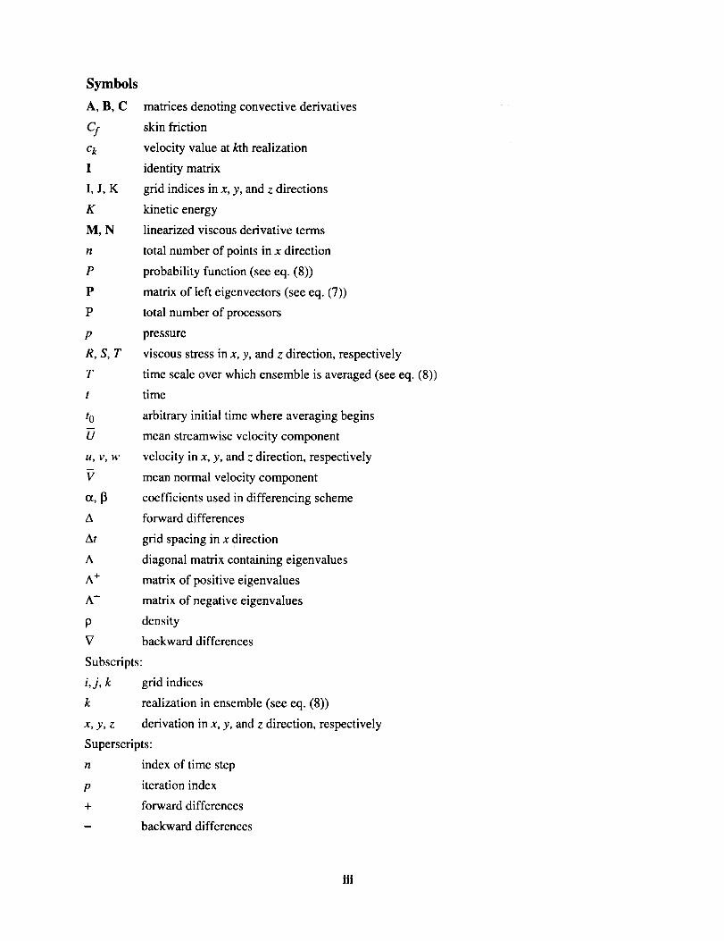
Symbols

A,B,C

clCk

I

I,J,K

K

M,N

rl

P

P

P

P

R,S,T

T

t

to

U

U, 12, W

_,f3

A

At

A

A +

A-

P

V

matrices denoting convective derivatives

skin friction

velocity value at kth realization

identity matrix

grid indices in x, y, and z directions

kinetic energy

linearized viscous derivative terms

total number of points in x direction

probability function (see eq. (8))

matrix of left eigenvectors (see eq. (7))

total number of processors

pressure

viscous stress in x, y, and z direction, respectively

time scale over which ensemble is averaged (see eq. (8))

time

arbitrary initial time where averaging begins

mean streamwise velocity component

velocity in x, y, and z direction, respectively

mean normal velocity component

coefficients used in differencing scheme

forward differences

grid spacing in x direction

diagonal matrix containing eigenvalues

matrix of positive eigenvalues

matrix of negative eigenvalues

density

backward differences

Subscripts:

i, j, k grid indices

k realization in ensemble (see eq. (8))

x, y, z derivation in x, y, and z direction, respectively

Superscripts:

n index of time step

p iteration index

+ forward differences

- backward differences

Ill

Abbreviations:

CFD

DNS

PIOFS

RISC

computational fluid dynamics

direct numerical simulation

parallel input/output file system

reduced instruction set computer

iv

Abstract

A distributed algorithm for a high-order-accurate finite-difference

approach to the direct numerical simulation (DNS) of transition and

turbulence in compressible flows is described. This work has two

major objectives. The first objective is to demonstrate that parallel and

distributed-memory machines can be successfully and efficiently used

to solve computationally intensive and input/output intensive algo-

rithms of the DNS class. The second objective is to show that the com-

putational complexity involved in solving the tridiagonal systems

inherent in the DNS algorithm can be reduced by algorithm innova-

tions that obviate the need to use a parallelized tridiagonal solver.

1. Introduction

Computational techniques such as direct numerical simulation (DNS) often have massive associated

memory requirements. Storage and computing time on traditional supercomputers are becoming

increasingly hard to obtain because of the prohibitive associated costs.

In recent years, computational fluid dynamics (CFD) techniques have been used successfully to

compute flows that are related to geometrically complex configurations. Currently, interest in the com-

putation of turbulent compressible flows has been revived to aid in the design of high-speed vehicles

and associated propulsion systems. Databases of compressible turbulent flows are not as readily avail-

able as those for incompressible turbulent flows. The effort described in this paper is the first parallel

application of DNS for a compressible, turbulent, supersonic spatially evolving boundary-layer flow.

A turbulent flow is simulated at moderate Reynolds numbers. A simulation at a moderate Reynolds

number can be used as a guide in understanding the fundamental turbulent physics of such flows and

can provide relevant Reynolds stress and dissipation rate budgets, which have been proved useful in the

incompressible studies.

The computational method used by Rai and Moin (ref. 1) is a high-order-accurate, upwind-biased,

implicit finite-difference method. The technique involves the use of upwind-biased differences for theconvective terms, central differences for the viscous terms, and an iterative implicit time-integration

scheme. The computational method uses the nonconservative form of the governing equations to obtainthe solution. This method has been shown in reference 2 to control the aliasing error through the natural

dissipation in the scheme but at the expense of some accuracy. However, this loss in accuracy can beovercome by increasing the number of grid points. In the present study, the method presented in refer-

ence 2 is extended to solve the compressible form of the Navier-Stokes equations.

The lack of efficient and accurate general tridiagonal solvers is a serious bottleneck in obtainingparallel solutions of problems that involve large tridiagonal systems, such as those in the DNS algo-

rithm. Existing parallel tridiagonal system solvers are limited in their applicability to matrices of partic-

ular forms, and their accuracies in the context of general tridiagonal systems are questionable. A

significant innovation in the present work is the elimination of the need for parallel tridiagonal solvers.

A novel algorithm has been developed to partition the tridiagonal system so that each node can solve its

own portion of the system with no sacrifice in accuracy. The scheme and the boundary conditions that

are employed herein are described in detail.

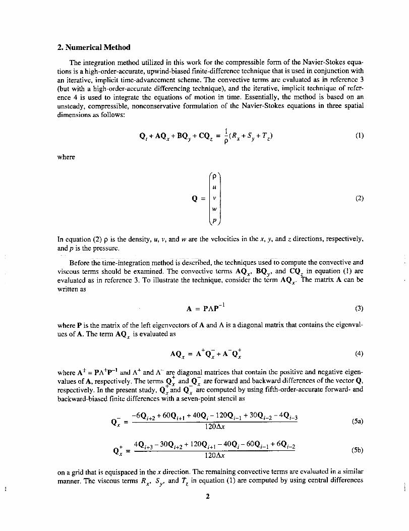
2. Numerical Method

The integration method utilized in this work for the compressible form of the Navier-Stokes equa-

tions is a high-order-accurate, upwind-biased finite-difference technique that is used in conjunction with

an iterative, implicit time-advancement scheme. The convective terms are evaluated as in reference 3

(but with a high-order-accurate differencing technique), and the iterative, implicit technique of refer-

ence 4 is used to integrate the equations of motion in time. Essentially, the method is based on an

unsteady, compressible, nonconservative formulation of the Navier-Stokes equations in three spatialdimensions as follows:

Qt + AQx + BQy + CQ z = _(R x + Sy + Tz) (l)

where

Q (2)

In equation (2) p is the density, u, v, and w are the velocities in the x, y, and z directions, respectively,

and p is the pressure.

Before the time-integration method is described, the techniques usedto compute the convective andviscous terms should be examined. The convective terms AQ , BQ , and CQ in equation (1) are

x y z

evaluated as in reference 3. To illustrate the technique, consider the term AQx. The matrix A can bewritten as

A = PAP -l (3)

where P is the matrix of the left eigenvectors of A and A is a diagonal matrix that contains the eigenval-

ues of A. The term AQ x is evaluated as

= A Qx+A QxAQ x + - _ + (4)

where A ± = PA±P --1 and A + and A- are diagonal matrices that contain the positive and negative eigen-

values of A, respectively. The terms +Q: and Qx are forward and backward differences of the vector Q,respectively. In the present study, Qx and Qx are computed by using fifth-order-accurate forward- andbackward-biased finite differences with a seven-point stencil as

-6Qi+2 + 60Qi+! + 40Qi - 120Qi_ 1 + 30Qi_ 2 - 4Qi_ 3Q: = 120Az (5a)

_+ 4Qi+3 - 30Qi+2 + 120Qi+l - 40Qi - 60Qi_l + 6Qi_ 2(Sb)

_"/x 120Ax

on a grid that is equispaced in the x direction. The remaining convective terms are evaluated in a similar

manner. The viscous terms R x, Sy, and Tz in equation (1) are computed by using central differences

anda five-pointstencil(fourth-orderaccuracy).Thefully implicit finite-differencerepresentationofequation(1)in factoredformisgivenby

+ A-Ax P aI

I + + +\ x, xj L L YJ

C+\ zk Azk )J (Qp+l_Qp)

l- M _ + - N __ZY

Ayj yj Vyy Ayj

=-At{ 3Qp-4Qn+Qn-I_-_ +( A+ -Qx +A- + B+-Qx + Qy

(6)

B-+ C+QT+C-Q+)"+ Qy +

where tx = 1.51t3, _ = 1.5 -2/3, V and A are backward and forward difference operations, respectively, the

matrices M and N represent the linearization of the first and second derivatives in the viscous terms, and

the superscript p is an iteration index. The factored form of equation (1) results in the systems of block-

tridiagonal matrices shown in equation (6). One additional approximation that has been made to the x

and z terms on the left-hand side of equation (6) is the use of the diagonal form as given in reference 5.

The inversion in the x direction is approximated as

o_I + 13At + = P txI + _At/--V---\ xi Ax i )J \ xi

+ A-Axllp-I

Ax i )J(7)

where the matrices P, p-l, and A are defined in equation (3). The approximation results in systems of

scalar tridiagonal equations instead of block-tridiagonal equations. The inversion in the z direction istreated in a similar manner.

3. Parallel Hardware Platform

This computation scheme was implemented on the 48-node IBM SP2 computer available at the

Langley Research Center. The IBM SP2 is a distributed-memory parallel computer that adopts a

message-passing communication paradigm and supports virtual memory. Each processor is functionallyequivalent to an IBM reduced instruction set computer (RISC) system/6000 deskside system with

128 Mb of local memory. The key component in all distributed-memory parallel computers is the inter-

connection network that links the processors together. The SP2 high-performance switch is a multistagepacket-switched omega network that provides a minimum of four paths between any pair of nodes in the

system.

4. Parallel Algorithm and Implementation

In the present work, the computation domain is split equally among processors along the stream-wise direction. The purpose of the data distribution strategy is to balance the load on the processors

and minimize communication between processors. In the physical domain, the coordinate directions

x (streamwise), y (normal), and z (spanwise) are associated with the indices I, J, and K, respectively.

The x direction has the largest number of points associated with it, and more importantly the gradients

of the flow quantities are small in this direction. Both the y and z directions have a much smaller numberof associated points. Moreover, the y direction, because it is the viscous direction, has very high

3

gradientsin its flow quantities.This largegradientcanintroducea largeerrorthatresultsfrom datatransferatthenodeboundaries.Thusthex direction was chosen for the data partitioning.

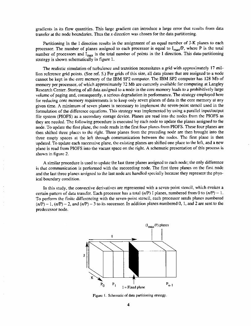
Partitioning in the I direction results in the assignment of an equal number of J-K planes to each

processor. The number of planes assigned to each processor is equal to Imax/P, where P is the total

number of processors and Imax is the total number of points in the I direction. This data-partitioning

strategy is shown schematically in figure 1.

The realistic simulation of turbulence and transition necessitates a grid with approximately 17 mil-

lion reference grid points. (See ref. 5.) For grids of this size, all data planes that are assigned to a node

cannot be kept in the core memory of the IBM SP2 computer. The IBM SP2 computer has 128 Mb of

memory per processor, of which approximately 72 Mb are currently available for computing at Langley

Research Center. Storing of all data assigned to a node in the core memory leads to a prohibitively large

volume of paging and, consequently, a serious degradation in performance. The strategy employed here

for reducing core memory requirements is to keep only seven planes of data in the core memory at any

given time. A minimum of seven planes is necessary to implement the seven-point stencil used in the

formulation of the difference equations. This strategy was implemented by using a parallel input/output

file system (PIOFS) as a secondary storage device. Planes are read into the nodes from the PIOFS as

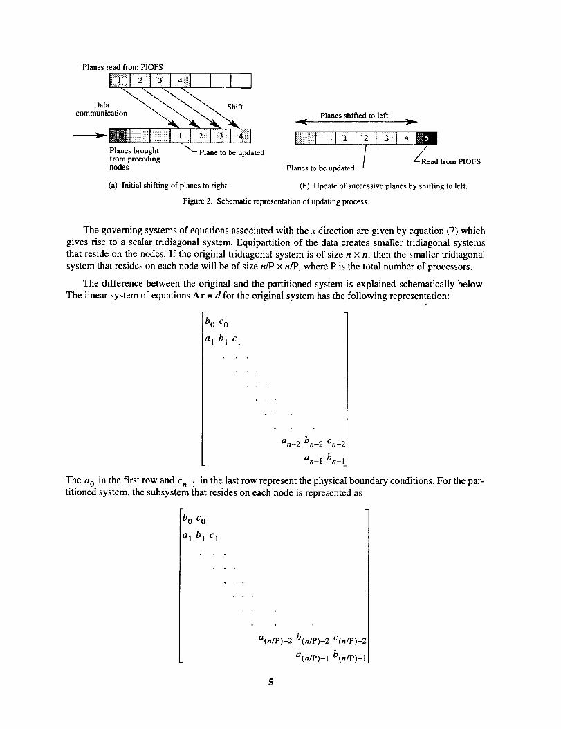
they are needed. The following procedure is executed by each node to update the planes assigned to the

node. To update the first plane, the node reads in the first four planes from PIOFS. These four planes are

then shifted three places to the right. Three planes from the preceding node are then brought into the

three empty spaces at the left through communication between the nodes. The first plane is then

updated. To update each successive plane, the existing planes are shifted one place to the left, and a new

plane is read from PIOFS into the vacant space on the right. A schematic presentation of this process is

shown in figure 2.

A similar procedure is used to update the last three planes assigned to each node; the only difference

is that communication is performed with the succeeding node. The first three planes on the first node

and the last three planes assigned to the last node are handled specially because they represent the phys-

ical boundary condition.

In this study, the convective derivatives are represented with a seven-point stencil, which evokes a

certain pattern of data transfer. Each processor has a total (n/P) I planes, numbered from 0 to (n/P) - 1.To perform the finite differencing with the seven-point stencil, each processor sends planes numbered

(n/P) - 1, (n/P) - 2, and (n/p) - 3 to its successor. In addition planes numbered 0, 1, and 2 are sent to the

predecessor node.

K

P0 PI

v

I = Fixed plane

(/max/P) planes

II

Pn- 1

Figure 1. Schematic of data-partitioning strategy.

Planes read from PIOFS

com

Planes brought Plane to be updatedfrom precedingnodes

(a) Initial shifting of planes to right.

Planes shifted to leftv

Planes to be updatedL Read from PIOFS

(b) Update of successive planes by shifting to left.

Figure 2. Schematic representation of updating process.

The governing systems of equations associated with the x direction are given by equation (7) which

gives rise to a scalar tridiagonal system. Equipartition of the data creates smaller tridiagonal systems

that reside on the nodes. If the original tridiagonal system is of size n x n, then the smaller tridiagonal

system that resides on each node will be of size n/P x n/P, where P is the total number of processors.

The difference between the original and the partitioned system is explained schematically below.

The linear system of equations Ax = d for the original system has the following representation:

bo Co

a I b 1 c 1

The a0 in the first row and Cn_ 1 in the last row represent the physical boundary conditions. For the par-

titioned system, the subsystem that resides on each node is represented as

b0 Co

a i b 1 c 1

a(n/P)-2 b(n/P)-2 C(nlP)-2

a(n/P)-I b(n/P)-I

For the first node, a 0 is a physical boundary condition; for all other nodes, a 0 must be brought in from

the predecessor node through the data communication.

Similarly for the last node, c .... is a physical boundary condition; for all other nodes C(nlP)_ 1tnlrl-I

must be brought in from the succeedmg processor through the data communication. Data needed from

neighboring nodes are immediately available because they are brought in through the communicationscheme. In the original, undivided problem, the most recent values of the point solutions are used in the

back substitution phase. In the distributed case, the node-interface boundary condition values retain

their values from the previous time step until a redistribution is accomplished at the next time step.

Therefore, a time lag occurs for solutions at the node boundaries. The resulting error can be driven

down if necessary by iterations per time step. In the original scheme implemented by Rai and Moin

(ref. 1), the performance of additional iterations was necessary at each time step to reduce the lineariza-tion error; thus, the number of iterations required to reduce the error at the boundary interfaces does not

significantly increase the computational cost.

The algorithmic innovations described have been shown to be an efficient method for the computa-

tions of memory-intensive problems such as the DNS formulation. Note that the goal of this paralleliza-

tion technique is to utilize distributed-memory machines to solve very large problems with considerable

memory requirements that exhaust the capabilities of traditional supercomputers. In this context, scaling

of the problem has no relevance; thus, timing studies are not warranted. Conventional performancestudies that use speedup comparisons are, therefore, not attempted in this work. Verification of the accu-

racy of the results obtained with the IBM SP2 machine is reported in the following section.

5. Validation

Although the procedure outlined previously has demonstrated a method for executing these

large-scale computations, the ultimate test is to verify that equivalent results can be obtained from theCRAY Y-MP and the IBM SP2 computers. Recently, a spatially developing, compressible, flat-plate

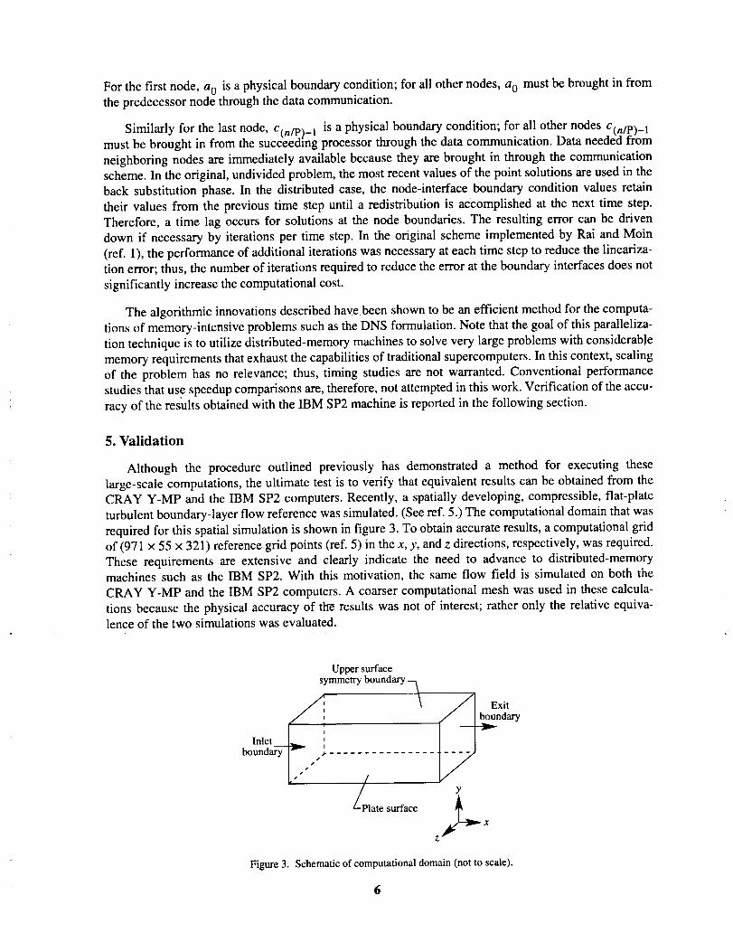
turbulent boundary-layer flow reference was simulated. (See ref. 5.) The computational domain that was

required for this spatial simulation is shown in figure 3. To obtain accurate results, a computational gridof (971 × 55 x 321 ) reference grid points (ref. 5) in the x, y, and z directions, respectively, was required.

These requirements are extensive and clearly indicate the need to advance to distributed-memorymachines such as the IBM SP2. With this motivation, the same flow field is simulated on both the

CRAY Y-MP and the IBM SP2 computers. A coarser computational mesh was used in these calcula-

tions because the physical accuracy of the results was not of interest; rather only the relative equiva-lence of the two simulations was evaluated.

Upper surface

symmetry boundary -_

Inlo, ou%y

y

b°undary F"" ""* Z//PPlatesurface z _ x

Figure 3. Schematic of computational domain (not to scale).

A fully turbulent flow is a stochastic system that is characterized by its statistical properties. At each

spatial location, every time step in the computational procedure is a single realization within a large

ensemble of events. Some flows, such as the wall-bounded flow considered here, have two useful prop-

erties: they are homogeneous in one spatial direction (z) and they are stationary. Thus in the z direction

a suitable spatial average over several integral scales yields a mean value that is independent of z; simi-lar results occur for a temporal average. Thus, effective comparisons between the simulations from each

machine can only be accomplished through comparisons of the statistical moments. An explanation ofthe first two moments, that is, the mean (first moment) and the variance (second central moment), issufficient.

For illustrative purposes, the instantaneous streamwise velocity is used to demonstrate how these

moments can be extracted. The time mean of the instantaneous streamwise velocity u(x,t), for example,is given by

U(x) = Z Uk(X'tk)P[tlCk-1 (x) <_U(x,t) < Ck(X)]k

(8)1 "to+T

= T---)_lim _ Jr0 U(x,t) dt

where P[tlCk_l(X)< U(x,t)<Ck(X)] is the probability that the function U(x,t) is delimited by

[ck_ l(x),ck(x)]. Because the process is assumed to be ergodic, the ensemble and time averages shownin equation (8) are equal. Analogous relationships also hold for the homogeneous spatial directions as

well. In turbulent flows for which the velocity field is stationary, the flow field customarily is decom-

posed into its mean and fluctuating parts which are given by

U(x,t) = U(x) + u(x,t) (9)

This decomposition is called a Reynolds decomposition and is interpreted as a partitioning of the flow

field into a deterministic mean-flow part and a random turbulent part. The turbulent part, thus, has zero

time mean (i.e., fi = 0). Given this property, the second central moment can be obtained in a straight-

forward manner from the following association with the turbulent part of the flow field:

u2(x) = U2(x,t)- U2(x) (10)

In the boundary-la!er flow considered here, the mean flow is two-dimensional, with mean velocitycomponents U and V that correspond to the x and y directions; the turbulence is always three-

dimensional with the components u, v, and w that correspond to the x, y, and z directions. In the analysis

of turbulent flows, most comparisons are based either on the mean streamwise velocity and the turbulentkinetic energy or on twice the variance of the total velocity field.

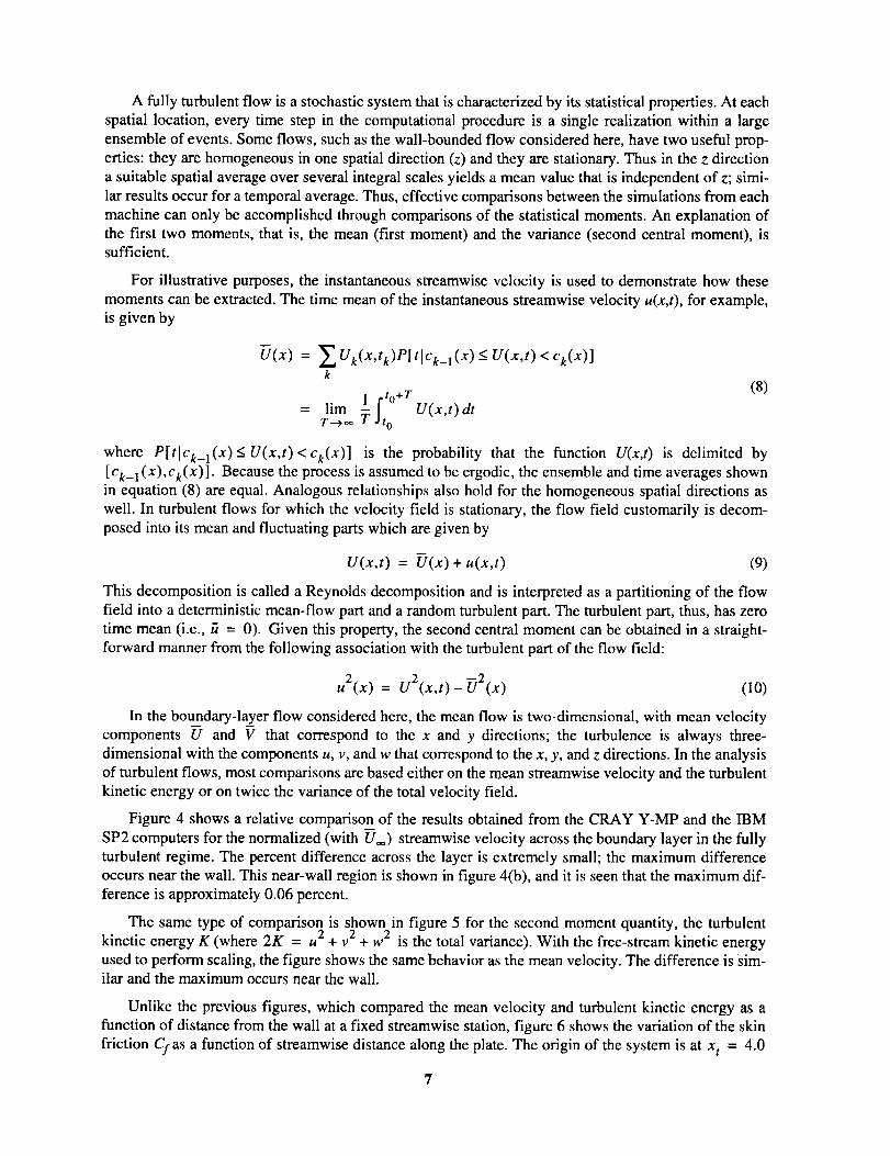
Figure 4 shows a relative comparison of the results obtained from the CRAY Y-MP and the IBM

SP2 computers for the normalized (with U_) streamwise velocity across the boundary layer in the fully

turbulent regime. The percent difference across the layer is extremely small; the maximum difference

occurs near the wall. This near-wall region is shown in figure 4(b), and it is seen that the maximum dif-

ference is approximately 0.06 percent.

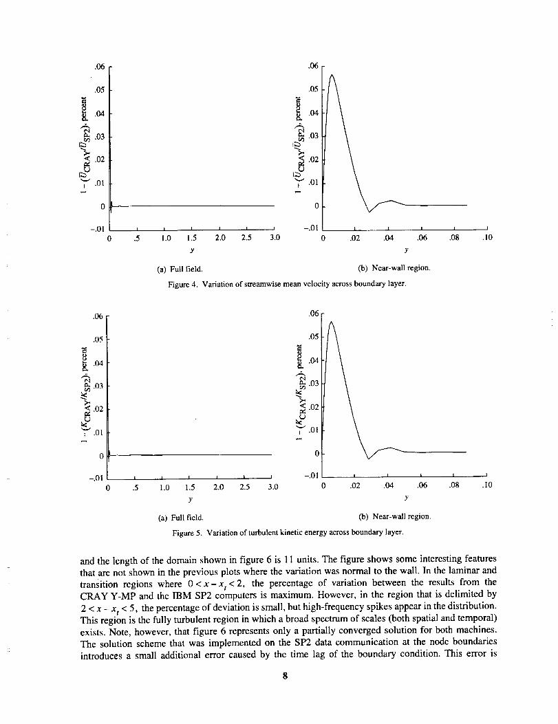
The same type of comparison is shown in figure 5 for the second moment quantity, the turbulent

kinetic energy K (where 2K = u 2 + v2 + w2 is the total variance). With the free-stream kinetic energy

used to perform scaling, the figure shows the same behavior as the mean velocity. The difference is sim-ilar and the maximum occurs near the wall.

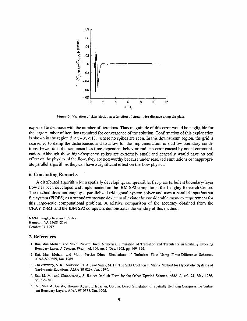
Unlike the previous figures, which compared the mean velocity and turbulent kinetic energy as a

function of distance from the wall at a fixed streamwise station, figure 6 shows the variation of the skin

friction Cf as a function of streamwise distance along the plate. The origin of the system is at x t = 4.0

7

.06

.05

.04

.03

.02

'_" .01

-.01

I

.06

.05

.04

.03

.02

.01

0

-.01I I I I I I I I I

0 .5 1.0 1.5 2.0 2.5 3.0 0 .06 .08 .10

Y

I I

.02 .04

Y

(a) Full field. (b) Near-wall region.

Figure 4. Variation of streamwise mean velocity across boundary layer.

.06

.05

.04

.03

"_ .02e_

"_ .01

-.01

.06

.05

..04

.03

.02

"_" .O1

-.01, I I I I I I I I I

0 .5 1.0 1.5 2.0 2.5 3.0 0 .06 .08 .I0

Y

! I

.02 .04

Y

(a) Full field. (b) Near-wall region.

Figure 5. Variation of turbulent kinetic energy across boundary layer.

and the length of the domain shown in figure 6 is 1 1 units. The figure shows some interesting features

that are not shown in the previous plots where the variation was normal to the wall. In the laminar and

transition regions where 0 < x- x t < 2, the percentage of variation between the results from the

CRAY Y-MP and the IBM SP2 computers is maximum. However, in the region that is delimited by

2 < X - x t < 5, the percentage of deviation is small, but high-frequency spikes appear in the distribution.

This region is the fully turbulent region in which a broad spectrum of scales (both spatial and temporal)

exists. Note, however, that figure 6 represents only a partially converged solution for both machines.

The solution scheme that was implemented on the SP2 data communication at the node boundaries

introduces a small additional error caused by the time lag of the boundary condition. This error is

.08

I I I I I I

2 4 6 8 10 12

X -- X l

Figure 6. Variation of skin friction as a function of streamwise distance along the plate.

expected to decrease with the number of iterations. Thus magnitude of this error would be negligible for

the large number of iterations required for convergence of the solution. Confirmation of this explanation

is shown in the region 5 < x - x t < 11, where no spikes are seen. In this downstream region, the grid iscoarsened to damp the disturbances and to allow for the implementation of outflow boundary condi-

tions. Fewer disturbances mean less time-dependent behavior and less error caused by nodal communi-

cation. Although these high-frequency spikes are extremely small and generally would have no real

effect on the physics of the flow, they are noteworthy because under resolved simulations or inappropri-

ate parallel algorithms they can have a significant effect on the flow physics.

6. Concluding Remarks

A distributed algorithm for a spatially developing, compressible, flat-plate turbulent boundary-layer

flow has been developed and implemented on the IBM SP2 computer at the Langley Research Center.

The method does not employ a parallelized tridiagonal system solver and uses a parallel input/outputfile system (PIOFS) as a secondary storage device to alleviate the considerable memory requirement for

this large-scale computational problem. A relative comparison of the accuracy obtained from the

CRAY Y-MP and the IBM SP2 computers demonstrates the validity of this method.

NASA Langley Research Center

Hampton, VA 23681-2199

October 23, 1997

7. References

1. Rai, Man Mohan, and Moin, Parviz: Direct Numerical Simulation of Transition and Turbulence in Spatially Evolving

Boundary Layer. J. Comput. Phys., vol. 109, no. 2, Dec. 1993, pp. 169-192.

2. Rai, Man Mohan; and Moin, Parviz: Direct Simulations of Turbulent Flow Using Finite-Difference Schemes.AIAA-89-0369, Jan. 1989.

3. Chakravarthy, S. R.; Anderson, D. A.; and Salas, M. D.: The Split Coefficient Matrix Method for Hyperbolic Systems ofGasdynamic Equations. AIAA-80-0268, Jan. 1980.

4. Rai, M. M.; and Chakravarthy, S. R.: An Implicit Form for the Osher Upwind Scheme. AIAA J., vol. 24, May 1986,pp. 735-743.

5. Rai, Man M.; Gatski, Thomas B.; and Erlebaeher, Gordon: Direct Simulation of Spatially Evolving Compressible Turbu-lent Boundary Layers. AIAA-95-0583, Jan. 1995.

9

Form ApprovedREPORT DOCUMENTATION PAGE OMBNo.0704-018e

Publicreportingburdenfor thiscollectionof informationIs estimatedto average1 hourperresponse,includingthe timefor revlewthginstructions,searchingexistingdata sources,gatheringand maintainingthe data needed,and completingandreviewingthe collectionof information.Sendcommentsregardingthisburden estimateor any otheraspectof this_ollectionof information,includingsuggestionsfor reducingthIsburden, to WashingtonHeadquartersServices,Directoratefor InformationOperationsand Reports,1215JeffersonDavisHighway,Suite 1204, Arlington,VA22202-4302, and to the Officeof Managementand Budget,PaperworkReductionProjesJ(0704-0188), Washington,DC 20503.

1. AGENCY USE ONLY (Leave blank) 2. REPORT DATE 3. REPORT TYPE AND DATES COVERED

December 1997 Technical Paper

4. TITLE AND SUBTITLE 5. FUNDING NUMBERS

Efficient Parallel Algorithm for Direct Numerical Simulation of TurbulentFlows WU 505-59-50

S. AUTHOR(S)

Stuti Moitra and Thomas B. Gatski

7. PERFORMING ORGANIZATION NAME(S) AND ADDRESS(ES)

NASA Langley Research Center

Hampton, VA 23681-2199

9. SPONSORING/MONITORING AGENCY NAME(S) AND ADDRESS(ES)

National Aeronautics and Space AdministrationWashington, DC 20546-0001

8. PERFORMING ORGANIZATIONREPORT NUMBER

L-17638

10. SPONSORING/MONITORINGAGENCY REPORT NUMBER

NASA TP-3686

11. SUPPLEMENTARY NOTES

12a. DISTRIBUTION/AVAILABILITY STATEMENT

Unclassified-Unlimited

Subject Category 34Availability: NASA CASI (301) 621-0390

12b. DISTRIBUTION CODE

13. ABSTRACT (Max/mum 200 words)

A distributed algorithm for a high-order-accurate finite-difference approach to the direct numerical simulation(DNS) of transition and turbulence in compressible flows is described. This work has two major objectives. Thefirst objective is to demonstrate that parallel and distributed-memory machines can be successfully and efficientlyused to solve computationally intensive and input/output intensive algorithms of the DNS class. The second objec-tive is to show that the computational complexity involved in solving the tridiagonal systems inherent in the DNSalgorithm can be reduced by algorithm innovations that obviate the need to use a parallelized tridiagonal solver.

14. SUBJECT TERMS

Direct numerical simulation 03NS); Parallel input/output file system (PIOFS);

Distributed memory; Message-passing

17. SECURITY CLASSIFICATIONOF REPORT

Unclassified

NSN 7540-01-280-5500

18. SECURITY CLASSIFICATIONOF THIS PAGE

Unclassified

19. SECURITY CLASSIRCATION

OF ABSTRACT

Unclassified

15. NUMBER OF PAGES

1516. PRICE CODE

A03

20. LIMITATIONOF ABSTRACT

Standard Form 298 (Rev. 2-89)PrescribedbyANSI Std.Z39-18298-102